Low-density Phase Diagram of the Three-Dimensional Electron Gas

Abstract

Variational and diffusion quantum Monte Carlo methods are employed to investigate the zero-temperature phase diagram of the three-dimensional homogeneous electron gas at very low density. Fermi fluid and body-centered cubic Wigner crystal ground state energies are determined using Slater-Jastrow-backflow and Slater-Jastrow many-body wave functions at different densities and spin polarizations in finite simulation cells. Finite-size errors are removed using twist-averaged boundary conditions and extrapolation of the energy per particle to the thermodynamic limit of infinite system size. Unlike previous studies, our results show that the electron gas undergoes a first-order quantum phase transition directly from a paramagnetic fluid to a body-centered cubic crystal at density parameter $r_{\text{s}}=86.6(7)$, with no region of stability for an itinerant ferromagnetic fluid.

I Introduction

The three-dimensional homogeneous electron gas (3D-HEG) has been of fundamental interest in physics and chemistry since the early days of quantum mechanics because it is the simplest realistic bulk electronic system capable of exhibiting strong correlation effects [1, 2, 3, 4, 5, 6]. The electron-electron interaction strength, and therefore the coupling between the electrons, is controlled by the electron density. The 3D-HEG models the electrons in bulk metals, but more importantly it has long provided a testbed for the development of ideas, concepts, and methods in condensed matter physics. For example, the ground-state energy of the 3D-HEG provides the starting point for most of the exchange-correlation functionals that have enabled the widespread success of density functional theory (DFT). In this work we focus on the low-density energy and phase behavior of the 3D-HEG.

Theory plays a crucial role in the study of dilute 3D-HEGs due to the lack of a material platform that supports a 3D electron system with both very high quality (homogeneity) and low density. It is convenient to characterize the density of the 3D-HEG by the dimensionless parameter $r_{\text{s}}$ defined as the radius of the sphere that contains one electron on average in units of the Bohr radius. In Hartree atomic units the 3D-HEG Hamiltonian is $\hat{H}=-(1/2)\sum_{i}\nabla_{i}^{2}+\sum_{i>j}1/|\mathbf{r}_{i}-\mathbf{r}_{j}|$, where $\mathbf{r}_{i}$ is the position of electron $i$ and the electron-electron Coulomb interaction is in practice evaluated using Ewald summation in a finite cell. The Coulomb interaction scales as $1/r_{\text{s}}$, while the kinetic energy operator scales as $1/r_{\text{s}}^{2}$. At high to intermediate density (small $r_{\text{s}}$) the kinetic energy dominates, leading to the well-known Fermi fluid behavior of the 3D-HEG at typical metallic densities. On the other hand, the Coulomb energy dominates the kinetic energy at low density (large $r_{\text{s}}$), fundamentally altering the physics of the 3D-HEG. In the low-density limit, the ground-state wave function is an antisymmetrized product of $\delta$-functions centered on body-centered cubic (bcc) lattice sites to minimize the Coulomb energy, as first predicted by Wigner [2]. Here, we calculate the critical density parameter $r_{\text{s}}$ at which there is a zero-temperature phase transition from a Fermi fluid to a Wigner crystal. Furthermore, Bloch suggested that the spin-unpolarized (paramagnetic) Fermi fluid should make a spontaneous transition to a spin polarized (ferromagnetic) Fermi fluid at large $r_{\text{s}}$ before crystallization [1], because aligning the electron spins causes the spatial wave function to be fully antisymmetric, so that electrons do not approach each other and the Coulomb energy is reduced.

Quantum Monte Carlo (QMC) methods have long been used to provide accurate estimates of properties of 3D-HEGs [7, 8, 9, 10, 11, 12, 13, 14]. For example, ground state QMC energies of the 3D-HEG [9] are employed in parameterizations of the local-density approximation to the DFT exchange-correlation functional [15]. However, calculating the phase diagram is challenging because of the tiny energy differences between competing phases. Previous QMC simulations have indicated that decreasing the density of a 3D-HEG causes a continuous transition from a spin-unpolarized (paramagnetic) fluid to a fully spin-polarized (ferromagnetic) fluid at a density of about $r_{\text{s}}=50(2)$ [11]. The phase transition to a Wigner crystal was predicted to take place at density parameter $r_{\text{s}}=106(1)$ [11, 16]. Because of the fundamental role of the 3D-HEG in condensed matter physics, the determination of its zero-temperature phase diagram and ground-state energy is a problem that should be revisited from time-to-time using state-of-the-art computational methods.

In this work we have used the continuum variational and diffusion Monte Carlo (VMC [17, 7] and DMC [9]) methods in real space to obtain 3D-HEG ground state energies at different densities and spin polarizations. In the VMC method, parameters in a trial wave function are optimized according to the variational principle, with energy expectation values calculated by Monte Carlo integration in the $3N$-dimensional space of electron position vectors. In the DMC method, the imaginary-time Schrödinger equation is used to evolve a statistical ensemble of electronic configurations towards the ground state. Fermionic antisymmetry is maintained by the fixed-phase approximation, in which the complex phase of the wave function is constrained to equal that of an approximate wave function optimized within VMC. For real wave functions (which occur when the system has time-reversal symmetry, e.g., under pure periodic boundary conditions), the fixed-phase approximation reduces to constraining the nodal surface of the wave function. Henceforth we refer to “fixed nodes” rather than “fixed phases” to avoid confusion with thermodynamic “phases”; our actual fluid calculations used complex wave functions and the fixed-phase approximation, while our crystal calculations used real wave functions and the fixed-node approximation.

Fixed-node DMC finds the variational lowest-energy state with the same nodal surface as the trial wave function. Thus the topology of the trial wave function’s nodal surface selects the quantum state under study. The DMC energy with an antisymmetric trial wave function is an upper bound on the fermionic ground-state energy; furthermore, the error in the DMC energy of any quantum state approximated by the trial wave function is second order in the error in the trial nodal surface.

In a finite cell the eigenfunctions of the 3D-HEG Hamiltonian must all be homogeneous (i.e., must satisfy the many-body Bloch theorems [18, 19] with an infinitesimal “primitive cell”) and hence eigenvalue crossings as a function of the single parameter $r_{\text{s}}$ are avoided by the von Neumann-Wigner theorem. The true ground state energy per electron $E(r_{\text{s}})$ of the 3D-HEG in a finite periodic cell of a given shape, electron number $N$, and spin-polarization $\zeta=(N_{\uparrow}-N_{\downarrow})/N$ is therefore a smooth function of $r_{\text{s}}$. The ground-state static structure factor $S({\bf G})=\left<\hat{\rho}(-{\bf G})\hat{\rho}({\bf G})\right>-\langle\hat{\rho}(-{\bf G})\rangle\langle\hat{\rho}({\bf G})\rangle$, where $\hat{\rho}({\bf G})=\sum_{i}\exp(i{\bf G}\cdot\hat{\bf r}_{i})$, describes the Fourier components of the pair density and therefore shows whether the 3D-HEG is fluid-like or crystal-like; this too is a smooth function of $r_{\text{s}}$ in a given finite cell. In fact there is a different $E(r_{\text{s}})$ curve for each system size $N$, spin polarization, cell shape, and choice of twisted boundary conditions. For example a bcc simulation cell with $N$ a cubic number strongly favors crystalline behavior. The fluid energy per particle fluctuates quasirandomly with system size $N$, cell shape, and twisted boundary conditions due to momentum quantization effects. For a sufficiently large periodic cell of a given shape, there must be a narrowly avoided crossing of energy levels as a function of $r_{\text{s}}$ near the crystallization density, with $S({\bf G}_{\text{prim}})$ changing significantly near the avoided crossing, where $\mathbf{G}_{\text{prim}}$ is a primitive-cell reciprocal lattice point of the bcc Wigner crystal, resulting in a smooth crossover from Fermi fluid to “floating” [20, 21] crystal behavior. For the infinite 3D-HEG, however, the center-of-mass kinetic energy per electron vanishes and hence broken-translational-symmetry crystal wave functions are degenerate with floating crystal wave functions. The avoided crossing of energy levels therefore becomes a true crossing of energy levels with different symmetry. Furthermore, $E(r_{\text{s}})$ ceases to depend on the simulation cell shape and choice of twisted boundary conditions. At $r_{\text{s}}\rightarrow 0$, the interaction potential is negligible and we have a homogeneous ground-state fluid wave function. At $r_{\text{s}}\to\infty$, the kinetic energy is negligible and we have a bcc crystal. The symmetry of the ground state of the infinite 3D-HEG must therefore change at some finite $r_{\text{s}}$, i.e., there is a zero-temperature phase transition [2]. The charge density $\rho({\bf G}_{\text{prim}})=\langle\hat{\rho}({\bf G}_{\text{prim}})\rangle$ is an appropriate order parameter for the fluid-to-crystal transition, being zero in the fluid phase and nonzero in the crystal phase. The crystallization transition is expected to be first order, corresponding to a crossing of crystal and fluid energy levels as functions of $r_{\text{s}}$ with the order parameter being nonzero at the crossing point in the crystal phase. The following numerical results provide some evidence confirming that the Wigner crystal charge density is nonzero at the crystallization density.

II Calculating the zero-temperature phase diagram

II.1 QMC methodology

In QMC studies of the phase diagram of the 3D-HEG, we look for a first-order phase transition by calculating the DMC energy as a function of density parameter $r_{\text{s}}$ for trial wave functions that model the ground-state fluid and the ground-state crystal. For the fluid phases we use Slater determinants of plane-wave orbitals, multiplied by Jastrow correlation factors that do not alter the nodal surface [7, 8, 9]. We evaluate the orbitals at quasiparticle coordinates related to the actual electron coordinates by continuous backflow (BF) transformations [22, 23, 24, 25], allowing variational optimization of the nodal surface without changing its topology. The nodal topology of the fluid trial wave function is therefore the same as that of a Slater determinant of plane waves, i.e., the wave function of a free electron gas. This model is not exact: as directly revealed by full configuration interaction QMC calculations, the exact ground-state wave function of the 3D-HEG is in fact a linear combination of many ground- and excited-state Slater determinants of plane waves [13, 26]. Nevertheless, the single-determinant Slater-Jastrow-BF (SJB) model of the fluid phase is reasonably accurate because, by construction, it always leads to a significantly lower variational energy than the Hartree-Fock wave function (a single determinant of plane waves), and Hartree-Fock theory itself becomes arbitrarily accurate at high density ($r_{\text{s}}\to 0$), where it provides the first two terms in the high-energy expansion of the 3D-HEG energy [27]. Furthermore, Landau’s Fermi liquid theory [4] requires that low-lying excited states of the Fermi fluid are adiabatically connected to the corresponding excited states of a free electron gas, implying that the relevant parts of the nodal surface of the Fermi fluid must be qualitatively the same as that of a single determinant of plane waves. The release-node method [9], in which walkers are equilibrated in fixed-node DMC and then briefly allowed to cross nodes and change the sign of their weights, is able to move nodes but is unlikely to be able to change the nodal topology; we expect this approach to give similar results to the fixed-node SJB-DMC method.

Our model of the Wigner crystal is a Slater determinant of single-Gaussian orbitals centered on bcc lattice sites and made periodic by summing over images, multiplied by a Jastrow correlation factor. It therefore explicitly breaks translational symmetry, leading to an $O(N^{-1})$ finite-size (FS) error due to the center-of-mass kinetic energy [28]. The Gaussian exponent was determined using a formula that minimizes the fixed-node DMC energy in a large 216-electron cell [16, 28]. The Slater determinant of Gaussian orbitals describes the ground state of an Einstein model of a vibrating electron lattice. In principle a better model of the ground state of a vibrating electron lattice would be provided by an antisymmetrized product of Gaussian functions of quasiharmonic normal coordinates [29, 30]. However, our Jastrow factor and BF function allow an approximate description of this quasiharmonic behavior, with additional flexibility.

Our Jastrow factor and BF functions contained polynomial and plane-wave expansions in electron-electron separation [31, 25]. For the Wigner crystal the Jastrow factor also contained a plane-wave expansion in electron position. The wave functions were optimized by variance minimization [32, 33] followed by energy minimization [34]. The casino package was used for all our QMC calculations [35].

Monte Carlo-sampled canonical twist-averaged boundary conditions (TABC) were used to reduce quasirandom single-particle FS errors in Fermi fluid energies due to momentum quantization effects [36, 37]. Twist averaging is unnecessary for Wigner crystals, which have localized orbitals and do not have Fermi surfaces. Systematic FS errors due to the use of the Ewald interaction rather than $1/r$ to evaluate the interaction between each electron and its exchange-correlation hole and the neglect of long-range two-body correlations were removed by fitting $E(N)=E(\infty)+b/N$ to the twist-averaged DMC energy data at different system sizes [38]. This also removed the FS bias in Wigner crystal energies due to the center-of-mass kinetic energy. We examine the performance of analytic expressions [38, 39].

We studied the fluid phase at $r_{\text{s}}=30$, 40, 50, 60, 70, 80, and 100. For each density, QMC calculations were performed for simulation cells with $130\leq N\leq 274$. The energies were calculated for spin polarizations $\zeta=0$, 0.25, 0.5, 0.75, and 1. Antiferromagnetic and ferromagnetic bcc crystalline phases were investigated at $r_{\text{s}}=80$, 90, 100, and 125 for simulation cells with $N=64$, 216, and 512 electrons. Our DMC energies were extrapolated linearly or quadratically to zero time step, with the target walker population being varied in inverse proportion to the time step. The energies and variances calculated using Slater-Jastrow (SJ) and SJB wave functions for different system sizes are reported in the Supplemental Material [28]. The computational and technical details are discussed in the following sections.

II.2 Fluid phase wave function

For the fluid phase of the three-dimensional homogeneous electron gas (3D-HEG) we used a Slater-Jastrow-backflow (SJB) trial spatial wave function $\Psi({\bf R})=e^{J({\bf R})}S({\bf X}({\bf R}))$, where ${\bf R}=({\bf r}_{1},\ldots,{\bf r}_{N})$ is the $3N$-dimensional vector of electron coordinates. The antisymmetric Slater part $S$ is a product of determinants of single-particle orbitals for spin-up and spin-down electrons. The single-particle orbitals in $S$ are of the free-electron form $\psi_{\mathbf{k}}(\mathbf{r})=\exp(i\mathbf{k}\cdot\mathbf{r})$, where wavevector $\mathbf{k}$ is a reciprocal lattice vector of the simulation cell offset by twist vector $\mathbf{k}_{\text{s}}$, where $\mathbf{k}_{\text{s}}$ lies in the supercell Brillouin zone. The Jastrow exponent $J$, which is symmetric under electron exchange, takes the form

$$J(\mathbf{R})=\sum_{i<j}^{N}u(r_{ij})+\sum_{i<j}^{N}p(\mathbf{r}_{ij}),$$ (1)

where $u$ is a smoothly truncated, isotropic polynomial function of minimum-image electron-electron distance $r_{ij}$, and $p$ is a plane-wave expansion in electron-electron separation ${\bf r}_{ij}$ [31]. The $u$ term is of form

$$u(r) = {(r-L_{u})}^{C}\Theta(L_{u}-r)$$ (2)

$${}\times\left(\alpha_{0}+\left[\frac{\Gamma}{{(-L_{u})}^{C}}+\frac{\alpha_{0}C}{L_{u}}\right]r+\sum_{l=2}^{N_{u}}\alpha_{l}r^{l}\right),$$

where the cutoff length $L_{u}$ is less than or equal to the radius of the largest sphere that can be inscribed in the Wigner-Seitz cell of the simulation cell, $C=3$ specifies how smooth the function is at the cutoff length, $\Theta$ is the Heaviside step function, and $\{\alpha_{l}\}$ are optimizable parameters, which differ for parallel- and antiparallel-spin electrons. To satisfy the Kato cusp conditions [40], $\Gamma=1/2$ for opposite-spin electrons and $\Gamma=1/4$ for same-spin electrons. We chose $N_{u}=8$. The $p$ term has the symmetry of the simulation-cell Bravais lattice and allows a description of correlation in the “corners” of the simulation cell. Its form is

$$p(\mathbf{r})=\sum_{A}a_{A}\sum_{\mathbf{G}\in A^{+}}\cos(\mathbf{G}\cdot\mathbf{r}),$$ (3)

where $A$ represents a star of symmetry-equivalent, nonzero, simulation-cell reciprocal-lattice vectors ${\bf G}$, and $A^{+}$ is a subset of $A$ that consists of one out of each $\pm{\bf G}$ pair. The $\{a_{A}\}$ are optimizable parameters. We used 46 stars of ${\bf G}$ vectors in $p$.

Including a backflow transformation in the trial wave function, the Slater part of the wave function $S$ is evaluated at transformed “quasiparticle” coordinates ${\bf X}(\mathbf{R})=\mathbf{R}+{\bm{\xi}}(\mathbf{R})$, where

$${\bm{\xi}}_{i}(\mathbf{R})=\sum_{j\neq i}^{N}\eta(r_{ij})\mathbf{r}_{ij}+\sum_{j\neq i}^{N}{\bm{\pi}}({\bf r}_{ij})$$ (4)

is the backflow displacement of electron $i$. $\eta$ is a cuspless, smoothly truncated, isotropic polynomial function of minimum-image electron-electron distance $r_{ij}$. The polynomial coefficients are optimizable parameters, and are different for parallel- and antiparallel-spin electrons [25]. The form of $\eta(r)$ is mathematically equivalent to that of the Jastrow $u(r)$ term [Eq. (2), with $\Gamma=0$ for same-spin electrons and optimizable for opposite-spin electrons]. Typically we used $N_{\eta}=8$ in the polynomial expansions. The ${\bm{\pi}}$ term has the form of the gradient of a Jastrow $p$ term [Eq. (3)]:

$${\bm{\pi}}({\bf r})=-\sum_{A}c_{A}\sum_{{\bf G}\in A^{+}}\sin({\bf G}\cdot{\bf r})\,{\bf G},$$ (5)

where the $c_{A}$ are optimizable parameters. As the gradient of a scalar field, the ${\bm{\pi}}$ term is irrotational. We used 44 stars of ${\bf G}$ vectors in ${\bm{\pi}}$. The backflow transformation preserves the antisymmetry of the Slater wave function. The parameters in the Jastrow factor and backflow function were optimized by variance minimization and energy minimization.

II.3 Crystal phase wave function

The trial wave functions for our Wigner crystal calculations were of later-Jastrow (SJ) form, apart from some test calculations with SJB wave functions. The orbitals in the Slater determinants consisted of Gaussian functions centered on body-centered cubic (bcc) lattice sites within the simulation cell, made periodic by summing over simulation-cell images:

$$\phi_{{\bf R}_{\text{p}}}({\bf r})=\sum_{{\bf R}_{\text{s}}}\exp\left(-C\left|{\bf r}-{\bf R}_{\text{p}}-{\bf R}_{\text{s}}\right|^{2}\right),$$ (6)

where ${\bf R}_{\text{p}}$ is a primitive-cell lattice point within the supercell (which indexes the orbital) and ${\bf R}_{\text{s}}$ is a simulation-cell lattice point. In practice the sum contained only those Gaussian functions $\exp\left(-C\left|{\bf r}-{\bf R}_{\text{p}}-{\bf R}_{\text{s}}\right|^{2}\right)$ whose value at the closest point to ${\bf R}_{\text{p}}+{\bf R}_{\text{s}}$ in the Wigner-Seitz simulation cell containing ${\bf r}$ was greater than $10^{-7}$. It was verified that truncating the sum in this manner does not introduce statistically significant errors at the densities considered in this work: see Table 1 and note that the effects of truncating the sum are reduced in larger simulation cells; our production Wigner crystal calculations used cell sizes of $N=64$, 216, and 512 electrons.

Table 1: Convergence of variational Monte Carlo (VMC) energy with respect to a parameter $g$ controlling the number of periodic images retained in the Wigner crystal orbitals of Eq. (6). We only retained those Gaussian functions $\exp\left(-C\left|{\bf r}-{\bf R}_{\text{p}}-{\bf R}_{\text{s}}\right|^{2}\right)$ whose value at the closest point of the Wigner-Seitz simulation cell containing ${\bf r}$ was greater than $10^{-g}$. Results are shown for a ferromagnetic bcc Wigner crystal at $r_{\text{s}}=90$ with $N=27$ electrons in the simulation cell and Gaussian exponent $C=0.000148$ a.u. An SJB wave function optimized with $g=7$ was used in each case.

$g$	No. terms in Eq. (6)	SJB-VMC energy (Ha/el.)
1	8	$-0.0084224(3)$
2	24	$-0.00849361(7)$
3	27	$-0.00849268(7)$
5	27	$-0.00849263(7)$
7	27	$-0.00849253(7)$
15	46	$-0.00849254(7)$
25	91	$-0.00849253(6)$

In Fig. 1 we plot diffusion Monte Carlo (DMC) energy against the logarithm of the Gaussian exponent $C$ for bcc Wigner crystals at $r_{\text{s}}=100$ and $r_{\text{s}}=125$. It is clear that the formula [16]

$$C=0.11r_{\text{s}}^{-3/2}$$ (7)

provides near-optimal exponents, especially for antiferromagnetic Wigner crystals. By using Eq. (7) we achieve greater consistency between system sizes and densities than would result from separately optimizing $C$ in each case. At small system size there is a tendency for $C$ to be underestimated relative to the thermodynamic limit, to reduce the center-of-mass kinetic energy. For both ferromagnetic and antiferromagnetic crystals the error in the DMC energy from using the formula is comparable with the statistical error bars on the data, and is clearly much smaller than the difference between the fluid and crystal energies, even at $r_{\text{s}}=100$, close to the crystallization density. A slightly more accurate expression for the optimal Gaussian exponent for ferromagnetic crystals would be $C_{\text{ferro}}=0.068r_{\text{s}}^{-3/2}$; however, for consistency, we have used Eq. (7) for all our production calculations. By contrast, within Hartree-Fock (HF) theory the low-density Gaussian exponent is $C_{\text{HF}}=1/(2r_{\text{s}}^{3/2})$ [16, 3].

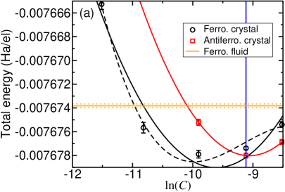
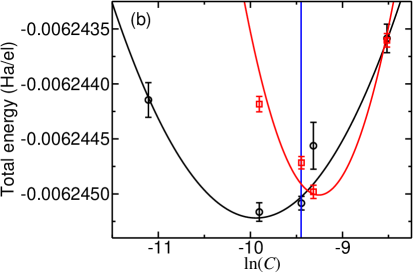
Figure 1: DMC energy against logarithm of Gaussian exponent $C$ for ferromagnetic and antiferromagnetic bcc Wigner crystals (a) at $r_{\text{s}}=100$ and (b) at $r_{\text{s}}=125$, using SJ trial wave functions. The energy has been extrapolated to zero time step and infinite system size in each case. The solid curves show quadratic fits to the energies of ferromagnetic and antiferromagnetic crystals as functions of $\ln(C)$, while the dashed curve shows a quartic fit. The horizontal line in (a) shows the twist-averaged paramagnetic Fermi fluid energy (with the dotted lines indicating error bars), while the vertical line shows the Gaussian exponent given by Eq. (7).

Our Wigner crystal Jastrow factors were of the same form as the Fermi fluid Jastrow factors described in the previous section, except that we used 7 stars of reciprocal lattice vectors in the plane-wave two-body term $p$, and we also used a plane-wave one-body term of the form

$$q(\mathbf{r})=\sum_{B}b_{B}\sum_{\mathbf{G}\in B^{+}}\cos(\mathbf{G}\cdot\mathbf{r}),$$ (8)

where $B$ represents a star of symmetry-equivalent, nonzero primitive-cell reciprocal-lattice vectors ${\bf G}$, and $B^{+}$ is a subset of $B$ that consists of one out of each $\pm{\bf G}$ pair. The $\{b_{B}\}$ are optimizable parameters. We used 7 stars of ${\bf G}$ vectors in $q$. The $q$ term has the symmetry of the Wigner crystal lattice and allows a description of anisotropic warping of the Gaussian orbitals.

For a ferromagnetic bcc Wigner crystal at $r_{\text{s}}=100$ with $N=64$ electrons, we performed test calculations using a backflow function of the form described in Sec. II.2, but with 8 stars in the ${\bm{\pi}}$ term. The VMC and DMC energies and the VMC variances obtained with SJ and SJB wave functions, using either Eq. (7) or VMC energy minimization to determine the orbital Gaussian exponent $C$, are shown in Table 2. Optimizing the Gaussian exponent and backflow function lower the VMC energy and variance. However, we cannot assume that optimizing an overall wave function leads to an improved nodal surface. In fact the DMC energies obtained using SJ and SJB wave functions and either Eq. (7) or VMC energy minimization to determine $C$ are all in statistical agreement with each other. Because SJ quantum Monte Carlo (QMC) calculations are much cheaper and allow us to explore larger system sizes, we have used SJ wave functions in our production calculations.

Table 2: VMC energy and variance and DMC energy for a ferromagnetic Wigner crystal at density parameter $r_{\text{s}}=100$ with $N=64$ electrons, using SJ and SJB wave functions and using either Eq. (7) or VMC energy minimization to determine the Gaussian orbital exponent $C$.

Wave function	$C$ (a.u.)	VMC energy (Ha/el.)	VMC variance (Ha2)	DMC energy (Ha/el.)
SJ	$0.00011$ [Eq. (7)]	$-0.0076719(3)$	$0.00000329$	$-0.00769616(8)$
SJ	$0.0001553$ (opt.)	$-0.0076737(2)$	$0.00000274$	$-0.0076957(2)$
SJB	$0.00011$ [Eq. (7)]	$-0.0076786(2)$	$0.00000252$	$-0.00769619(9)$
SJB	$0.0001503$ (opt.)	$-0.0076803(2)$	$0.00000201$	$-0.0076960(1)$

II.4 Finite-size effects in fluid phases

For twist averaging we used random twists $\{\mathbf{k}_{\text{s}}\}$ rather than a grid of twists for the following reasons. (i) Using random twists is similar to adding three more dimensions to the $3N$-dimensional integrals evaluated in QMC, and Monte Carlo integration is efficient in high-dimensional spaces. (ii) A truly systematic approach to twist averaging should use ${\bf k}_{\text{s}}$ in each supercell Brillouin zone (BZ) defined by the reoccupancies of the plane-wave orbitals, and the corresponding results should be weighted by the size of that BZ. However, the complexity of the nested BZs grows very rapidly with the number of electrons $N$ [36], making this approach infeasible for large system sizes. On the other hand, a regular grid-based approach effectively gives a random sampling of the nested BZs. (iii) Monte Carlo sampling of $\mathbf{k}_{\text{s}}$ is easily extensible: if the error is too large, it can be reduced by including more random twists.

To twist average, we used the HF kinetic energy ($T_{\text{HF}}$) and exchange energy ($X_{\text{HF}}$) as correlators and fit

$$E({\bf k}_{\text{s}}) = \langle E\rangle_{\text{TA}}+c\left[T_{\text{HF}}({\bf k}_{\text{s}})-\left<T_{\text{HF}}\right>_{\text{TA}}\right]$$ (9)

$${}+d\left[X_{\text{HF}}({\bf k}_{\text{s}})-\left<X_{\text{HF}}\right>_{\text{TA}}\right]$$

to the DMC energy per particle at a given system size, where ${\bf k}_{\text{s}}$ is the twist, and $\langle E\rangle_{\text{TA}}$, $c$, and $d$ are fitting parameters. The twist-averaged (TA) HF energies $\left<T_{\text{HF}}\right>_{\text{TA}}$ and $\left<X_{\text{HF}}\right>_{\text{TA}}$ are cheap to evaluate and were obtained using billions of twists.

Analytical expressions have been derived for the leading-order [38] and next-to-leading-order [39] systematic finite-size (FS) corrections to the energy per particle of a 3D homogeneous electron gas in a finite periodic cell in which the interaction between the particles is of Ewald form and the system is assumed to be well-described by a SJ wave function. The leading-order and next-to-leading-order FS corrections to the energy per electron of a Fermi fluid are

$$\Delta E=\frac{\sqrt{3}}{2Nr_{\text{s}}^{3/2}}-\frac{C_{\text{3D}}}{\pi r_{\text{s}}^{2}{(2N)}^{4/3}}\left[{(1+\zeta)}^{2/3}+{(1-\zeta)}^{2/3}\right],$$ (10)

where $C_{\text{3D}}=5.083$ in a face-centered cubic simulation cell (for fluid phases) and $5.086$ in a bcc simulation cell (for crystal phases). As explained in Ref. 41, backflow correlations lead to additional, negative $O(r_{\text{s}}^{-2}N^{-1})$ FS corrections to the energy per particle, approximately given by $\Delta E_{\text{BF}}=-T_{\text{HF}}/(3N)$, where $T_{\text{HF}}$ is the HF kinetic energy per particle. There is also a nonsystematic FS error in the canonical ensemble TA energy per particle of a Fermi fluid due to the incorrect shape of the TA Fermi surface; this error has an envelope that decays as $O(r_{\text{s}}^{-2}N^{-4/3})$ [36].

It is reasonable to assume that Eq. (10) holds approximately for Wigner crystals, although the static structure factor differs between fluids and crystals, so the corrections should not really be exactly the same.

The TA SJB-DMC energy of a paramagnetic Fermi fluid at $r_{\text{s}}=100$ is plotted against the reciprocal of system size in Fig. 2. The results of adding in the leading-order correction of Eq. (10) and the leading-order plus next-to-leading-order FS corrections are also shown. At these low densities the next-to-leading-order correction is negligible in comparison with the leading-order correction (and also the backflow correction is relatively small). Nevertheless, the leading-order FS correction does not remove all the systematic FS errors. Near the crystallization density the single-determinant wave function form is increasingly inappropriate, and it is possible that other FS effects may be present in the correlations implicitly described by DMC. It is clear from Fig. 2 that the leading-order analytic corrections do not remove all FS effects at $r_{\text{s}}=100$. We therefore believe the most accurate treatment of systematic FS effects is to extrapolate to infinite system size using the $O(N^{-1})$ FS-error scaling implied by the leading-order theory.

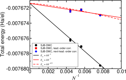
Figure 2: TA SJB-DMC energy against inverse of system size for a paramagnetic Fermi fluid at $r_{\text{s}}=100$. Also shown are the effects of applying the first and second terms of Eq. (10), and the effects of fitting various FS scaling laws to the resulting data.

The SJ-DMC energy of a ferromagnetic Wigner crystal at $r_{\text{s}}=100$ is plotted against system size in Fig. 3. It appears that the leading-order $O(N^{-1})$ behavior is not completely eliminated by either the long-range FS correction of Eq. (10) or the subtraction of the center-of-mass kinetic energy. Equation (10) was derived for a fluid phase; the static structure factor and long-range two-body Jastrow factor are different in a crystal phase, which would lead to a different prefactor. Once again the best policy would appear to be to regard the theory of FS effects as providing the appropriate scaling law to fit to the data.

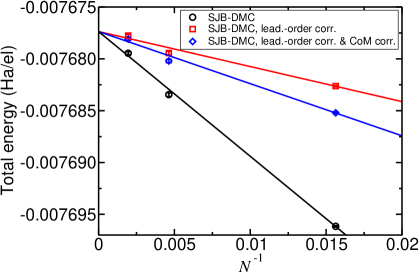
Figure 3: SJ-DMC energy against inverse of system size for a ferromagnetic bcc Wigner crystal at $r_{\text{s}}=100$. Also shown are the effects of applying the first term of Eq. (10) and of subtracting an estimate of the center-of-mass kinetic energy, together with fits of $E(N)=E(\infty)+bN^{-1}$ to the resulting energy data.

SJ-DMC energies as functions of system size $N$ for different spin polarizations ($\zeta=0$, 0.25, 0.5, 0.75, and 1) are illustrated in Fig. 4.

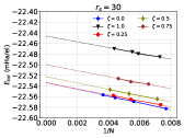
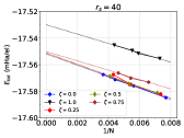
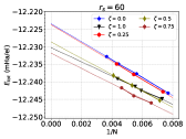
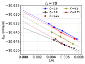
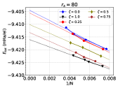
Figure 4: TA Fermi fluid SJ-DMC energies as functions of system size $N$ at different spin polarizations $\zeta$. The dotted line represents the extrapolation to infinite system size. These SJ-DMC energies have not been extrapolated to zero time step.

The SJ-DMC energies in the infinite system size limit for different densities and polarizations are listed in Table 3.

Table 3: TA SJ-DMC energy of the Fermi fluid extrapolated from different system sizes ($130<N<274$) with 300 random twists at each $N$ to the thermodynamic limit. Energies are in mHa/el. The numbers in parentheses indicate statistical errors. The DMC energies were not extrapolated to zero time step.

	0.0	0.25	0.50	0.75	1.0
30	$-22.5336(7)$	$-22.534(3)$	$-22.522(1)$	$-22.500(4)$	$-22.446(3)$
40	$-17.5518(4)$	$-17.551(4)$	$-17.552(1)$	$-17.550(2)$	$-17.523(1)$
50	$-14.4003(4)$	$-14.4034(1)$	$-14.4046(4)$	$-14.407(2)$	$-14.399(1)$
60	$-12.2235(2)$	$-12.2237(1)$	$-12.2286(1)$	$-12.231(2)$	$-12.2303(8)$
70	$-10.6278(5)$	$-10.629(1)$	$-10.6310(4)$	$-10.634(3)$	$-10.6374(5)$
80	$-9.404(1)$	$-9.406(1)$	$-9.4101(6)$	$-9.413(1)$	$-9.4161(5)$

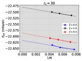
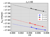
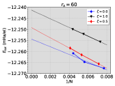
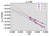
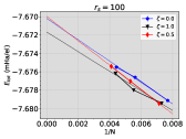
Figure 5: TA SJB-DMC energies against system size $N$ for different spin polarizations $\zeta$. The dotted lines represent extrapolations to infinite system size. The DMC energies were not extrapolated to zero time step.

The TA SJB-DMC energies of the fluid phase for various density and polarization are plotted in Fig. 5 against system size. The SJB-DMC energies extrapolated to infinite system are presented in Table 4.

Table 4: TA SJB-DMC energies of the Fermi fluid extrapolated to the thermodynamic limit from different system sizes ($130<N<274$). Energies are in mHa/el. The numbers in parentheses indicate statistical errors. The DMC energies were not extrapolated to zero time step.

	0.0	0.50	1.0
30	$-22.617(8)$	$-22.5862(5)$	$-22.4804(6)$
40	$-17.612(4)$	$-17.597(2)$	$-17.555(2)$
60	$-12.254(3)$	$-12.2492(4)$	$-12.2413(1)$
80	$-9.4250(9)$	$-9.421(1)$	$-9.4242(2)$
100	$-7.6702(4)$	$-7.669976(7)$	$-7.6717(9)$

II.5 Finite-size effects in crystal phases

In our broken-symmetry model of a Wigner crystal there is an additional FS error due to the center-of-mass kinetic energy.

At low density, individual electrons occupy Gaussian orbitals $\phi_{{\bf R}_{\text{p}}}({\bf r})=\exp(-C|{\bf r}-{\bf R}_{\text{p}}|^{2})$, where ${\bf R}_{\text{p}}$ is a bcc primitive-cell lattice vector, and $C$ is a Gaussian exponent. Let ${\bf s}$ be the offset to the center-of-mass position. Assuming a rigid displacement of the lattice by ${\bf s}$, the center-of-mass wave function is $\Phi({\bf s})=\exp(-NCs^{2})$. The resulting center-of-mass kinetic energy is

$$T_{\text{CM}}=-\frac{1}{2N}\frac{\int\Phi^{*}\nabla_{\bf s}^{2}\Phi\,d^{3}{\bf s}}{\int|\Phi|^{2}\,d^{3}{\bf s}}=\frac{3C}{2}.$$ (11)

Hence the center of mass kinetic energy per particle falls off as $3C/(2N)$. There is therefore an additional FS correction, on top of those discussed in Sec. II.4, to be applied to the energy per particle of a Wigner crystal:

$$\Delta T_{\text{CM}}=-\frac{T_{\text{CM}}}{N}=-\frac{3C}{2N}\approx-\frac{0.33}{2Nr_{\text{s}}^{3/2}},$$ (12)

where in the last step we have inserted the approximate expression for the Gaussian exponent $C$ in a bcc Wigner crystal obtained by minimizing the DMC energy in a large simulation cell [16], Eq. (7). The center-of-mass kinetic energy correction partially offsets the leading-order FS correction of Eq. (10).

Where the crystal orbitals are highly localized within the supercell, twist averaging cannot have much effect on the energy per particle. If the simulation-cell Bloch vector ${\bf k}_{\text{s}}$ is nonzero then the crystal orbitals are

$$\phi_{{\bf R}_{\text{p}}}({\bf r})=\sum_{{\bf R}_{\text{s}}}\exp\left(-C\left|{\bf r}-{\bf R}_{\text{p}}-{\bf R}_{\text{s}}\right|^{2}\right)\exp\left(i{\bf k}_{\text{s}}\cdot{\bf R}_{\text{s}}\right),$$ (13)

where ${\bf R}_{\text{p}}$ is a primitive-cell lattice point within the supercell (which indexes the orbital) and ${\bf R}_{\text{s}}$ is a simulation-cell lattice point. This is the usual prescription for creating Bloch orbitals from localized functions; one can easily check that $\phi_{{\bf R}_{\text{p}}}({\bf r}+{\bf R}_{\text{s}}^{\prime})=\exp(i{\bf k}_{\text{s}}\cdot{\bf R}_{\text{s}}^{\prime})\phi_{{\bf R}_{\text{p}}}({\bf r})$.

For a large simulation cell at low density, at most one of the Gaussian functions $\exp\left(-C\left|{\bf r}-{\bf R}_{\text{p}}-{\bf R}_{\text{s}}\right|^{2}\right)$ in Eq. (13) is non-negligible at any given point ${\bf r}$ in the simulation cell. So the $\exp(i{\bf k}_{\text{s}}\cdot{\bf R}_{\text{s}})$ factor just contributes an unobservable phase to each orbital within the simulation cell. Hence we do not twist average our crystal energies.

The SJ-DMC energies of ferromagnetic Wigner crystals at different densities $r_{\text{s}}=80$, 90, 100, and 125 as functions of system size are plotted in Fig. 6. The energies extrapolated to infinite system size are listed in Table 5.

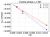
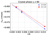
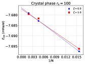
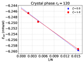
Figure 6: SJ-DMC energy against the inverse of system size $N$ for the crystal phase. The dotted line shows the extrapolation to infinite system size. $\zeta=0$ and 1 are the spin polarizations of the system (antiferromagnetic and ferromagnetic crystals, respectively). The DMC energies have been extrapolated to zero time step.

Table 5: SJ-DMC energy of the crystal phase extrapolated to zero time step and the thermodynamic limit of infinite system size. The numbers in parentheses indicate statistical and fitting errors.

	Energy (mHa/el.)
$r_{\text{s}}$	Antiferromagnetic	Ferromagnetic
80	$-9.4200(2)$	$-9.41999(9)$
90	$-8.4585(1)$	$-8.4581(1)$
100	$-7.6769(1)$	$-7.6774(1)$
125	$-6.24472(6)$	$-6.24508(6)$

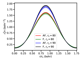
Figure 7: Extrapolated estimates of the electronic charge densities of antiferromagnetic (AF) and ferromagnetic (F) bcc Wigner crystals plotted along a straight line in the $[100]$ direction. Results are shown for two density parameters in the vicinity of the crystallization density. The charge densities have been obtained by extrapolated estimation (twice the DMC charge density minus the VMC charge density), which largely removes errors that are linear in the error in the trial wave function. Furthermore, the charge densities have been extrapolated to infinite system size, assuming the FS error goes as $N^{-1}$. The shaded regions indicate one standard error about the mean.

The electronic charge densities of antiferromagnetic and ferromagnetic crystals are plotted in Fig. 7. The charge densities were extrapolated to infinite system size by fitting $\rho_{\infty}({\bf r})+b({\bf r})N^{-1}$ to the charge density data $\rho_{N}({\bf r})$ at each point ${\bf r}$. Here, $\rho_{\infty}({\bf r})$ and $b({\bf r})$ were fitting parameters at each point $\mathbf{r}$. $O(N^{-1})$ FS errors in the charge density arise due to the center-of-mass kinetic energy, which leads to a tendency for the orbitals to delocalize in a finite cell.

It is clear that the charge density is nonuniform at the crystallization density, providing some numerical evidence that the phase transition is first order. The differences between ferromagnetic and antiferromagnetic crystals are too small to resolve, but it is clear that increasing $r_{\text{s}}$ has the effect of making the charge density relatively localized, as expected.

II.6 DMC time-step bias

The variation of the DMC energy with time step is investigated in this section. Figure 8 shows TA SJB-DMC energies against time step. The population is varied in inverse proportion to the time step. For all the studied system sizes, densities, and spin polarizations the bias at finite time step is always positive. Our final results were linearly extrapolated to zero time step (and hence infinite population) in every case.

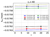
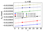
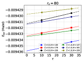
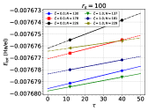
Figure 8: TA SJB-DMC energy against time step $\tau$ for the paramagnetic ($\zeta=0$) and ferromagnetic ($\zeta=1$) fluid phases at different system sizes $N$.

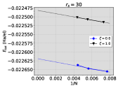
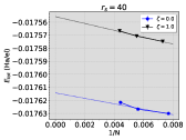
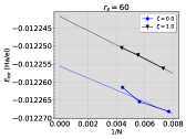
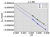
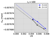
Figure 9: TA SJB-DMC energies against system size $N$ for different spin polarizations $\zeta$. The DMC energies are extrapolated to zero time step. The dotted line represents the extrapolation to infinite system size.

Figure 9 shows SJB-DMC energies of paramagnetic and ferromagnetic fluid phases, extrapolated to zero time step, at three different system sizes.

Table 6: TA SJB-DMC energies of the fluid phases of the 3D-HEG extrapolated to the thermodynamic limit from different system sizes ($130<N<274$). Energies are in mHa/el. The numbers in parentheses indicate statistical errors. The DMC energies were extrapolated to zero time step.

	0.0	1.0
30	$-22.6191(7)$	$-22.4819(7)$
40	$-17.6143(3)$	$-17.5558(7)$
60	$-12.2556(3)$	$-12.2418(5)$
80	$-9.4259(4)$	$-9.4246(3)$
100	$-7.6709(3)$	$-7.6720(4)$

TA SJB-DMC energies extrapolated to infinite system size and zero time step are listed in Table 6.

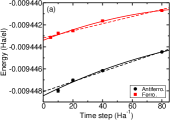
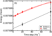
Figure 10: SJ-DMC energy against time step for bcc Wigner crystals at (a) $r_{\text{s}}=80$ and (b) $r_{\text{s}}=100$. Results are shown for both antiferromagnetic and ferromagnetic crystals. The system size is $N=64$ electrons. The target population is varied in inverse proportion to the time step.

The SJ-DMC energy of bcc Wigner crystals is plotted against time step in Fig. 10. Time steps in the range 10–80 Ha^-1 were used in our calculations. At $r_{\text{s}}=80$ the data are better fitted by a quadratic function of time step than a linear function of time step; however, the quadratic fit is no better than the linear fit at $r_{\text{s}}=100$. However, even at $r_{\text{s}}=80$, the difference between the results of linear and quadratic time-step extrapolation is not statistically significant.

III Results and discussion

III.1 SJ-DMC magnetic phase diagram for the fluid phases

The SJ-DMC phase diagram (Fig. 11, left panel) shows that the spin polarized state $\zeta=0.5$ has lower energy than the paramagnetic phase at $r_{\text{s}}\geqslant 40$. The fluid with $\zeta=0.75$ becomes more stable than the fluid with $\zeta=0.5$ at $r_{\text{s}}\approx 46$, and the 3D-HEG system adopts a fully polarized state $\zeta=1$ at $r_{\text{s}}\approx 62$.

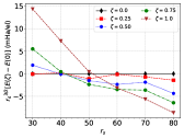
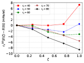
Figure 11: (Left panel) SJ-DMC spin polarization energy of the 3D-HEG multiplied by $r_{\text{s}}^{3/2}$ against density parameter $r_{\text{s}}$. (Right panel) SJ-DMC spin polarization energy of the 3D-HEG multiplied by ${r_{\text{s}}}^{3/2}$ against spin polarization $\zeta$ at various densities.

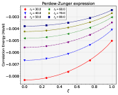
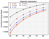
Figure 12: Correlation energies obtained in SJ-DMC calculations for the fluid phase (symbols), together with the fit to Eq. (1) of the main text (lines). Error bars on the QMC data are shown, but are smaller than the symbols. The DMC energies were not extrapolated to zero time step.

Table 7: Parameters in Eq. (2) of the main text, obtained by fitting to SJ-DMC data that have been TA and extrapolated to infinite system size, but not to zero time step.

$\zeta$	$\gamma$	$\beta_{1}$	$\beta_{2}$	$\chi^{2}$
0.0	$-0.122(5)$	$0.923(45)$	$0.287(10)$	$1.25$
0.25	$-0.104(7)$	$0.758(67)$	$0.252(15)$	$10.573$
0.5	$-0.110(5)$	$0.937(51)$	$0.275(10)$	$3.137$
0.75	$-0.091(14)$	$0.938(189)$	$0.250(36)$	$0.412$
1.0	$-0.052(5)$	$0.808(97)$	$0.166(13)$	$6.58$

The correlation energy of a Fermi fluid is defined as the difference between the Hartree-Fock energy per electron and the exact ground-state energy per electron, where the latter is approximated by our DMC results. The procedure developed by von Barth and Hedin [42] and Perdew and Zunger [15] to interpolate between $\zeta=0$ and $\zeta=1$ was applied to our SJ-DMC correlation energies (Fig. 12, top panel). The well-known Perdew-Zunger expression for the correlation energy per electron of the 3D-HEG is [15]

$$E_{\text{c}}(r_{\text{s}},\zeta)=E_{\text{c}}^{\text{para}}(r_{\text{s}})+\left[E_{\text{c}}^{\text{ferro}}(r_{\text{s}})-E_{\text{c}}^{\text{para}}(r_{\text{s}})\right]f(\zeta),$$ (14)

which has the same $\zeta$-dependence as the exchange energy [42], $f(\zeta)=\frac{{(1+\zeta)}^{4/3}+{(1-\zeta)}^{4/3}-2}{2\left(2^{1/3}-1\right)}$. This interpolation is exact for the exchange part of the energy and is likely to be reasonable for the correlation energy too. The interpolation scheme is very successful at low densities, as illustrated in Fig. 12.

Following Ceperley [8] we fit

$$E_{\text{c}}^{\text{para,ferro}}(r_{\text{s}})=\frac{\gamma^{\text{para,ferro}}}{1+\beta_{1}^{\text{para,ferro}}\sqrt{r_{\text{s}}}+\beta_{2}^{\text{para,ferro}}r_{\text{s}}}$$ (15)

to our Fermi fluid correlation energies.

The fitting parameters $\gamma$, $\beta_{1}$, and $\beta_{2}$ for different polarizations are listed in Table 7.

III.2 SJB-DMC magnetic phase diagram for the fluid phases

According to our SJB-DMC results for the fluid phases, the paramagnetic fluid phase ($\zeta=0$) is stable for the entire density range $r_{\text{s}}<85.5(2)$ (Fig. 13, left panel). There is no room for stability of the partially polarized $\zeta=0.5$ fluid phase.

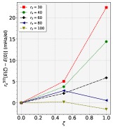
Figure 13: (Left panel) SJB-DMC relative energies of fluid phases of the 3D-HEG are plotted against $r_{\text{s}}$ for different spin polarizations $\zeta$ in the thermodynamic limit of infinite system size. (Right panel) SJB spin polarization energy of the 3D-HEG multiplied by ${r_{\text{s}}}^{3/2}$ at various densities. The DMC energies were not extrapolated to zero time step.

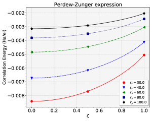
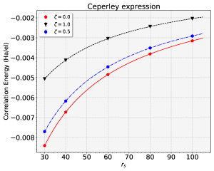
Figure 14: Correlation energies obtained in SJB-DMC calculations for the fluid phase (symbols), together with the fit of Eq. (14) (lines). Error bars on the QMC data are shown, but are smaller than the size of the symbols.

Figure 14 shows the SJB-DMC correlation energy of the fluid phase as a function of spin polarization at different densities. BF correlations lower the energy of the paramagnetic fluid more than the ferromagnetic fluid. SJ-DMC predicts that a fully spin-polarized fluid phase becomes stable at $r_{\text{s}}=63(1)$, whereas our SJB-DMC results do not show a statistically significant region for the ferromagnetic fluid phase. Same-spin electrons are kept apart by the antisymmetry of the many-body wave function, while opposite-spin electrons are only separated by correlation effects, so that an accurate treatment of correlations lowers the energies of paramagnetic phases more than ferromagnetic phases. Hence any future improvements in QMC trial wave functions are expected further to stabilize the paramagnetic fluid relative to spin-polarized fluids. In a Wigner crystal electrons are kept apart by the localization of orbitals on lattice sites, so there is relatively little scope for BF correlations to lower the DMC energy significantly. Indeed, the DMC energy data in the Supplemental Material confirm that the effects of BF on Wigner crystal DMC energies are small and do not significantly alter the phase diagram [28]. Our final energies are obtained using SJB-DMC for Fermi fluid phases and SJ-DMC for Wigner crystal phases.

Table 8: Parameters in the interpolation formula of Eq. (15) for the correlation energy of a Fermi fluid, obtained by fitting to our SJB-DMC energy data at different spin polarizations $\zeta$. The reduced $\chi^{2}$ values for the fits are also shown.

$\zeta$	$\gamma$ (Ha/el)	$\beta_{1}$	$\beta_{2}$	$\chi^{2}$
$0$ (para.)	$-0.13(1)$	$1.0(1)$	$0.32(3)$	$0.92$
$0.5$	$-0.15(1)$	$1.3(1)$	$0.36(2)$	$10.96$
$1$ (ferro.)	$-0.062(6)$	$0.97(8)$	$0.19(1)$	$5.51$

III.3 Phase diagram

The DMC energies of different phases of the 3D-HEG, extrapolated to the thermodynamic limit, are plotted against $r_{\text{s}}$ in Fig. 15. Our Wigner crystal energies are in good agreement with the results reported in Ref. 16. However, our Fermi fluid energies are substantially higher than those of Ref. 11, leading to a significant revision of the crystallization density, which is now predicted to occur at $r_{\text{s}}=86.6(7)$. We investigate possible reasons for the disagreement with Ref. 11 in the next section, finding that the treatment of finite-size effects is the most likely source of disagreement.

The ferromagnetic fluid becomes more stable than the paramagnetic fluid in the immediate vicinity of the crystallization density; hence we do not predict a region of stability for itinerant ferromagnetism in the 3D-HEG. The absence of a region of stability for the ferromagnetic fluid has also recently been predicted by Holzmann and Moroni, who performed DMC calculations for the fluid phases of the 3D-HEG in a 66-electron simple cubic cell and applied finite-size corrections to their data [43].

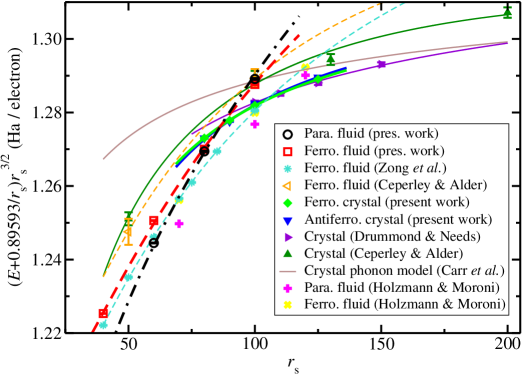
Figure 15: Energies per particle of the Fermi fluid and Wigner crystal phases at low density. The Madelung energy of the bcc lattice has been subtracted off and the resulting energies have been rescaled by $r_{\text{s}}^{3/2}$ to highlight the differences between phases.

The curves fitted to our DMC energy data for ferromagnetic and antiferromagnetic bcc crystals cross at $r_{\text{s}}=93(3)$, which is just inside the region of stability for the Wigner crystal. However, in the region of stability, the differences between our ferromagnetic and antiferromagnetic crystal DMC energies are statistically insignificant.

Path integral Monte Carlo calculations of the exchange coupling constants of bcc Wigner crystals [44] show that at $r_{\text{s}}=100$ the energy difference between ferromagnetic and antiferromagnetic configurations is only $1.2\times 10^{-8}$ Ha/el (an order of magnitude smaller than our DMC error bars), and demonstrate that the 3D Wigner crystal is antiferromagnetic [45]. Given that the energy difference between antiferromagnetic and ferromagnetic crystals is significant at high density and exponentially small at low density, fitted energy-density curves are liable to cross spuriously.

III.4 Investigation of disagreement with F. H. Zong, C. Lin, and D. M. Ceperley, Phys. Rev. E 66, 036703 (2002) (Ref. 11)

As can be seen in Fig. 15, our SJB-DMC energies in the thermodynamic limit are higher than those of Ref. 11. Here we try to identify the cause of the disagreement.

According to Ref. 11, the energy of a paramagnetic ($\zeta=0$) 3D-HEG at $r_{\text{s}}=40$ computed using TA SJB-DMC simulations and extrapolated to the thermodynamic limit from $N=54$ and $N=108$ is $-0.0176187(3)$ Ha/el. To try to reproduce this result we used SJB wave functions for the paramagnetic ($\zeta=0$) 3D-HEG at $r_{\text{s}}=40$ and the same system sizes as Ref. 11. The DMC time step was 10 Ha^-1. We used 1200 walkers for $N=54$ and 2400 walkers for $N=108$. The numbers of twists for $N=54$ and $N=108$ were 700 and 110, respectively. Our DMC energy at the thermodynamic limit, which is obtained by extrapolation of the TA DMC energies in Table 9, is $-0.0176038(1)$ Ha/el. This is 14.9(3) $\mu$Ha/el. higher than the result obtained in Ref. 11.

Table 9: Energies and energy variances (${\sigma_{\text{v}}}^{2}$) of the paramagnetic ($\zeta=0$) 3D-HEG at $r_{\text{s}}=40$. The TA DMC energies are calculated using an SJB wave function in which the Jastrow factor and backflow function were optimized at ${\bf k}_{\text{s}}={\bf 0}$. Energies are in Ha/el. and variances are in Ha².

$N$	$E_{\rm VMC}$	${\sigma_{\text{v}}}^{2}$	$E_{\rm DMC}$
$54$	$-0.0175860(9)$	$0.0000553(6)$	$-0.01766933(6)$
$108$	$-0.0175770(5)$	$0.0000898(8)$	$-0.01763656(7)$

To investigate further, we have studied $54$-electron 3D-HEGs at $r_{\text{s}}=50$ with the same set of spin polarizations as Ref. 11. We used our SJB wave function with several hundred twists to reach a precision of $10^{-7}$ Ha/electron. Figure 16 shows our VMC and DMC energies compared with data extracted from Fig. 1 of Ref. 11. Because they used a three-body term in their Jastrow factor, their VMC energies are $\sim 0.02$ mRy/electron lower than our VMC energies. However, the three-body Jastrow term does not directly affect the nodal surface of the wave function and indeed our DMC energies agree well with those of Ref. 11. We performed two test calculations in which a polynomial three-body term was included in our Jastrow factor. The resulting SJB-VMC energies for the paramagnetic and ferromagnetic fluid phases are $-0.028913(1)$ and $-0.028906(1)$ Ry/electron, respectively, which are lower than the corresponding VMC energies of Ref. 11 (see Fig. 16). However, including the three-body term did not change our DMC energies significantly. Indeed, Fig. 16 shows that the source of the discrepancy between our final SJB-DMC results and those of Ref. 11 is neither the form of our trial wave function nor the optimization scheme, because the SJB-DMC results agree at $N=54$.

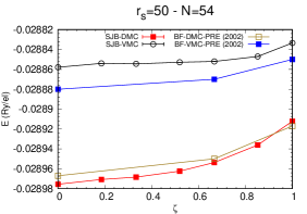
Figure 16: Twist-averaged SJB-VMC and SJB-DMC energies per electron $E$ against spin polarization $\zeta$ at $r_{\text{s}}=50$ for $N=54$ electrons. Our results were obtained using a face-centered cubic simulation cell. The results reported in Ref. 11 [“PRE (2002)”] may have been obtained in a simple cubic simulation cell, although the difference between the ground-state energies in face-centered and simple cubic cells is small, as shown in Table 11.

We calculated the energy of the 3D-HEG at $r_{\text{s}}=50$ in the infinite system size limit using TA and extrapolation from data at $N=54$ and $N=108$; these are the system sizes used in Ref. 11. According to Ref. 11, the TA SJB-DMC energies of paramagnetic fluids at $r_{\text{s}}=50$ at a system size of $N=54$ and at the thermodynamic limit are $-0.028967(1)$ and $-0.0288990(6)$ Ry/electron, respectively. Hence they find the absolute difference between the SJB-DMC energy at infinite system size and in a 54-electron cell to be just 0.068(1) mRy/electron.

Our SJB-DMC energies of the paramagnetic fluid at $r_{\text{s}}=50$ at a system size $N=54$ and at the thermodynamic limit are $-0.0289755(1)$ and $-0.0288756(4)$ Ry/electron, respectively, and the absolute difference between them is 0.1000(4) mRy/electron, much larger than predicted in Ref. 11.

According to Ref. 38, the leading order correction for systematic long-range FS errors in the energy is $\Delta_{N}=\omega_{\text{p}}/(2N)=\sqrt{3/r_{\text{s}}^{3}}/(2N)$ in atomic units, where $\omega_{\text{p}}=\sqrt{3/r_{\text{s}}^{3}}$ is the plasma frequency. Using $N=54$ and $r_{\text{s}}=50$ gives $\Delta_{N}=0.09072$ mRy/electron, which is relatively close to our estimate of the difference between the energy per particle at infinite system size and in a 54-electron cell.

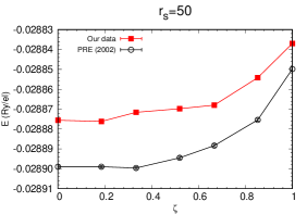
Figure 17: Energy per electron as a function of spin polarization $\zeta$ at $r_{\text{s}}=50$. The energies are obtained using extrapolation from TA energies at $N=54$ and $N=108$ to infinite system size.

Figure 17 compares our DMC energies with those of Ref. 11 for 3D-HEGs at $r_{\text{s}}=50$ in the thermodynamic limit. The differences between our DMC energies and those of Ref. 11 at $\zeta=0.0$, 0.185, 0.333, 0.519, 0.667, 0.852, and 1.0 are 0.023(7), 0.023(7), 0.0280(7), 0.0247(6), 0.0203(6), 0.0212(9), and 0.013(1) mRy/electron, respectively.

We investigated other factors that could affect our DMC energies:

• We reoptimized the backflow function and Jastrow factor at different twist vectors ${\bf k}_{\text{s}}$ for the paramagnetic fluid. The SJB-DMC energies at infinite system size, which are obtained by extrapolation from TA data at $N=54$ and $N=108$, show that the energy change due to optimizing the backflow function at different twists is small (see Table 10).

  Table 10: SJB-DMC energy in Ha/electron of a paramagnetic fluid at $r_{\text{s}}=50$ in the thermodynamic limit of infinite system size ($N\rightarrow\infty$) using three different simulation-cell Bloch vectors ${\bf k}_{\text{s}}$ for the optimization of the backflow function and Jastrow factor. The SJB-DMC energies were obtained by extrapolation from TA SJB-DMC energies obtained at system sizes of $N=54$ and $N=108$.

  	SJB-DMC energy (Ha/electron)
  		$\zeta=0$			$\zeta=1$
  ${\bf k}_{\text{s}}$	$N=54$	$N=108$	$N\rightarrow\infty$	$N=54$	$N=108$	$N\rightarrow\infty$
  $\Gamma$	$-0.0144877(1)$	$-0.0144628(1)$	$-0.0144378(1)$	$-0.0144561(2)$	$-0.0144373(3)$	$-0.0144185(3)$
  $L$	$-0.0144870(1)$	$-0.0144627(1)$	$-0.0144383(1)$	$-0.0144553(2)$	$-0.0144369(3)$	$-0.0144185(3)$
  $X$	$-0.0144866(1)$	$-0.0144622(1)$	$-0.0144378(1)$	$-0.0144555(2)$	$-0.0144366(3)$	$-0.0144178(3)$

• All the results of this section were obtained with a fixed DMC time step $\tau=10$ a.u., which is appropriately small at density parameter $r_{\text{s}}=50$. As shown in Sec. II.6, the resulting time step errors are much smaller than the difference between our energy data and those of Ref. 11.

• The shape of the simulation cell affects the DMC energy at finite system size. We used face centered cubic (fcc) simulation cells for our fluid calculations. It is not clear to us what shape of simulation cell was used in Ref. 11. $N=54$ is a magic number of electrons for paramagnetic 3D-HEGs in both simple cubic (sc) and fcc cells subject to periodic boundary conditions. We compare TA SJB-DMC energies for the paramagnetic fluid phase in fcc and sc cells at $r_{\text{s}}=50$ in Table 11. The difference between these DMC energies in the thermodynamic limit is negligible, as expected.

  Table 11: TA SJB-DMC energy of the paramagnetic fluid phase at $r_{\text{s}}=50$ using fcc and sc simulation cells. Energies are in Ha/electron.

  Simulation cell	$N=54$	$N=108$	$N\rightarrow$ $\infty$
  fcc	$-0.0144878(1)$	$-0.0144628(1)$	$-0.0144378(1)$
  sc	$-0.0144832(1)$	$-0.0144592(1)$	$-0.0144352(1)$

Since our SJB-DMC results agree with Ref. 11 at $N=54$ but not in the thermodynamic limit, and since Ref. 11 states that finite-size effects are small in contradiction with the analytic theory of finite-size effects [38], we conclude that FS extrapolation is the most likely cause of the disagreement between our results and Ref. 11.

III.5 Comparison with M. Holzmann and S. Moroni, Phys. Rev. Lett. 124, 206404 (2020) (Ref. 43)

Reference 43 disagrees with Ref. 11 and agrees with our finding that the ferromagnetic fluid has no region of stability. Nevertheless, there remains a quantitative disagreement over the crystallization density. Reference 43 uses computationally expensive recursive backflow wave functions in SJB-DMC calculations at a fixed, relatively small system size ($N=66$, in an sc cell). Furthermore, they extrapolate their SJB-DMC energy data to zero VMC energy variance. In general such an extrapolation is error-prone, possibly introducing nonvariational errors (consider, for example, the effects of switching between optimizing wave functions by variance and energy minimization); however, in Ref. 43 great care has been taken to ensure the extrapolation is as reliable as possible. On the other hand, rather than extrapolating energy data to infinite system size, Ref. 43 relies on analytic FS correction formulas.

In Table 12 we compare our TA SJB-DMC energies for the paramagnetic 66-electron Fermi fluid in a sc cell at $r_{\text{s}}=100$ with the results reported in Ref. 43. Our (nonrecursive) SJB trial wave function gives a lower TA DMC energy than their nonrecursive SJB wave function (“BF0” in Table 12). However, the recursion of backflow transformations followed by extrapolation to zero VMC variance results in lower TA SJB-DMC energies than ours. This difference between the fluid energies in our work and Ref. 43 is sufficient to explain about half the difference between the predicted crystallization densities [$r_{\text{s}}=86.6(7)$ and 113(2), respectively]. The rest of the difference can be ascribed to the fact that we extrapolate to infinite system size from larger simulation cells.

Table 12: TA SJB-DMC energies for a 66-electron paramagnetic Fermi fluid of density parameter $r_{\text{s}}=100$ in a sc cell. The results without citation were obtained in the present work. “BF$n$” denotes an SJB wave function obtained using $n$ recursive backflow transformations.

Trial wave function	SJB-DMC energy (mRy/el.)
BF0 [43]	$-15.37588(9)$
No 3-body Jastrow term	$-15.37721(11)$
With 3-body Jastrow term	$-15.37810(8)$
BF1 [43]	$-15.38345(7)$
BF4 [43]	$-15.38683(4)$
Extrap. to zero var. [43]	$-15.38914(17)$

IV Conclusion

In conclusion, we have revisited the phase diagram of the 3D-HEG using state-of-the-art QMC methods. The energies of Wigner crystals are similar to previous QMC calculations. However, we find ferromagnetic fluid energies that are significantly higher than previous calculations, leading to a higher crystallization density, at $r_{\text{s}}=86.6(7)$. We find no statistically significant region of stability for itinerant ferromagnetism. The zero-temperature phase diagram of the 3D-HEG is therefore found to be qualitatively similar to that of the two-dimensional homogeneous electron gas [46].

- [1] F. Bloch, Z. Phys. 57, 545 (1929).
- [2] E. Wigner, Phys. Rev. 46, 1002 (1934).
- [3] E. P. Wigner, Trans. Faraday. Soc. 34, 678 (1938).
- [4] L. D. Landau, Sov. Phys. JETP 8, 70 (1959).
- [5] D. Pines and P. Noziéres, The Theory of Quantum Liquids, W. A. Benjamin, Inc., New York, (1966).
- [6] G. Giuliani and G. Vignale, Quantum Theory of the Electron Liquid, Cambridge University Press, ISBN:9780511619915 (2005).
- [7] D. Ceperley, G. V. Chester, and M. H. Kalos, Phys. Rev. B 16, 3081 (1977).
- [8] D. Ceperley, Phys. Rev. B 18, 3126 (1978).
- [9] D. M. Ceperley and B. J. Alder, Phys. Rev. Lett. 45, 566 (1980).
- [10] G. Ortiz, M. Harris, and P. Ballone, Phys. Rev. Lett. 82, 5317 (1999).
- [11] F. H. Zong, C. Lin, and D. M. Ceperley, Phys. Rev. E 66, 036703 (2002).
- [12] G. G. Spink, N. D. Drummond, and R. J. Needs, Phys. Rev. B 88, 085121 (2013).
- [13] J. J. Shepherd, G. Booth, A. Grüneis, and A. Alavi, Phys. Rev. B 85, 081103(R) (2012)
- [14] S. Azadi, N. D. Drummond, and W. M. C. Foulkes, Phys. Rev. Lett. 127, 086401 (2021)
- [15] J. P. Perdew and A. Zunger, Phys. Rev. B 23, 5048 (1981).
- [16] N. D. Drummond, Z. Radnai, J. R. Trail, M. D. Towler, and R. J. Needs, Phys. Rev. B 69, 085116 (2004).
- [17] C. J. Umrigar, J. Toulouse, C. Filippi, S. Sorella, and R. G. Hennig, Phys. Rev. Lett. 98, 110201 (2007).
- [18] G. Rajagopal, R. J. Needs, S. Kenny, W. M. C. Foulkes, and A. James, Phys. Rev. Lett. 73, 1959 (1994).
- [19] G. Rajagopal, R. J. Needs, A. James, S. D. Kenny, and W. M. C. Foulkes, Phys. Rev. B 51, 10591 (1995).
- [20] R. F. Bishop and K. H. Lührmann, Phys. Rev. B 26, 5523 (1982).
- [21] M. Lewin, E. H. Lieb, and R. Seiringer, Phys. Rev. B 100, 035127 (2019).
- [22] R. P. Feynman and M. Cohen, Phys. Rev. 102, 1189 (1956).
- [23] M. A. Lee, K. E. Schmidt, M. H. Kalos, and G. V. Chester, Phys. Rev. Lett. 46, 728 (1981).
- [24] Y. Kwon, D. M. Ceperley, and R. M. Martin, Phys. Rev. B 58, 6800 (1998)
- [25] P. López Ríos, A. Ma, N. D. Drummond, M. D. Towler, and R. J. Needs, Phys. Rev. E 74, 066701 (2006).
- [26] M. Ruggeri, P. López Ríos, and A. Alavi, Phys. Rev. B 98, 161105(R) (2018).
- [27] M. Gell-Mann and K. A. Brueckner, Phys. Rev. 106, 364 (1957).
- [28] QMC raw data for all the system sizes studied are presented in the Supplemental Material.
- [29] W. J. Carr, Phys. Rev. 122, 1437 (1961).
- [30] W. J. Carr, R. A. Coldwell-Horsfall, and A. F. Fein, Phys. Rev. 124, 747 (1961).
- [31] N. D. Drummond, M. D. Towler, and R. J. Needs, Phys. Rev. B 70, 235119 (2004).
- [32] C. J. Umrigar, K. G. Wilson, and J. W. Wilkins, Phys. Rev. Lett. 60, 1719 (1988).
- [33] N. D. Drummond and R. J. Needs, Phys. Rev. B 72, 085124 (2005).
- [34] J. Toulouse and C. J. Umrigar, J. Chem. Phys. 126, 084102 (2007).
- [35] R. J. Needs, M. D. Towler, N. D. Drummond, P. López Ríos, and J. R. Trail, J. Chem. Phys. 152, 154106 (2020).
- [36] C. Lin, F. H. Zong, and D. M. Ceperley, Phys. Rev. E 64, 016702 (2001).
- [37] S. Azadi and W. M. C. Foulkes, Phys. Rev. B 100, 245142 (2019).
- [38] S. Chiesa, D. M. Ceperley, R. M. Martin, and M. Holzmann, Phys. Rev. Lett. 97, 076404 (2006).
- [39] N. D. Drummond, R. J. Needs, A. Sorouri, and W. M. C. Foulkes, Phys. Rev. B 78, 125106 (2008).
- [40] T. Kato, Commun. Pure Appl. Math. 10, 151 (1957); R. T. Pack and W. B. Brown, J. Chem. Phys. 45, 556 (1966).
- [41] M. Holzmann, R. C. Clay, III, M. A. Morales, N. M. Tubman, D. M. Ceperley, and C. Pierleoni, Phys. Rev. B 94, 035126 (2016).
- [42] U. von Barth and L. Hedin, J. Phys. C, 5, 1629 (1972).
- [43] M. Holzmann and S. Moroni, Phys. Rev. Lett. 124, 206404 (2020).
- [44] L. Cândido, B. Bernu and D. M. Ceperley, Phys. Rev. B 70, 094413 (2004).
- [45] D. J. Thouless, Proc. Phys. Soc. 86, 893 (1965).
- [46] N. D. Drummond and R. J. Needs, Phys. Rev. Lett. 102, 126402 (2009).