Signature of the gluon orbital angular momentum

Abstract

We propose a novel observable for the experimental detection of the gluon orbital angular momentum (OAM) that constitutes the proton spin sum rule. We consider longitudinal double spin asymmetry in exclusive dijet production in electron-proton scattering and demonstrate that the $\cos\phi$ azimuthal angle correlation between the scattered electron and proton is a sensitive probe of the gluon OAM at small-$x$ and its interplay with the gluon helicity. We also present a numerical estimate of the cross section for the kinematics of the Electron-Ion Collider.

1. Introduction—After more than 20 years of operation, the Relativistic Heavy Ion Collider (RHIC) spin program at Brookhaven National Laboratory has revealed that the gluon helicity contribution $\Delta G$ to the proton spin sum rule

$$\frac{1}{2}=\frac{1}{2}\Delta\Sigma+\Delta G+L_{q}+L_{g},$$ (1)

is nonvanishing and likely sizable STAR:2014wox ; deFlorian:2014yva ; Nocera:2014gqa ; Ethier:2017zbq ; STAR:2021mqa . Together with the known quark helicity contribution $\Delta\Sigma\sim 0.3$, the result indicates that parton helicities account for a significant fraction of the proton spin. Yet, there still remain huge uncertainties about the small-$x$ contribution to $\Delta G=\int_{0}^{1}dx\Delta G(x)$ defined as the first moment of the polarized gluon distribution function. Resolving this issue is one of the major goals of the future Electron-Ion Collider (EIC) AbdulKhalek:2021gbh .

Another obvious goal of the EIC is to measure the orbital angular momentum (OAM) of quarks and gluons $L_{q,g}$. However, progress in this direction is relatively slow although there have been continuing theory efforts (for recent works, see, e.g., Boussarie:2019icw ; Kovchegov:2019rrz ; Engelhardt:2020qtg ; Guo:2021aik ). Currently, there does not seem to be a consensus in the community about which observables need to be measured at the EIC in order to constrain $L_{q,g}$. This is so even after the first wave of proposals for experimental observables appeared several years ago Ji:2016jgn ; Hatta:2016aoc ; Bhattacharya:2017bvs ; Bhattacharya:2018lgm ; Guo:2021aik (see also an earlier attempt Courtoy:2013oaa ). These works exploit the known connection Lorce:2011kd ; Hatta:2011ku ; Lorce:2011ni between parton OAMs and the Wigner distributions Belitsky:2003nz , or equivalently, the generalized transverse momentum dependent distributions (GTMDs). However, the required processes typically involve very exclusive final states which are challenging to measure. Besides, observables are often related to GTMDs via complicated multi-dimensional convolutions even at the leading order. Clearly, more theoretical efforts are needed to increase the accuracy of predictions or devise new observables better suited for the purpose.

With this in mind, we take a fresh look at the process considered in Refs. Ji:2016jgn ; Hatta:2016aoc . There, the authors have proposed to measure longitudinal single spin asymmetry (SSA) in exclusive dijet production in electron-proton collisions $ep\to\gamma^{*}p\to jjp^{\prime}$ where the incoming proton is longitudinally polarized. It has been shown that the following angular-dependent part of the cross section

$$d\sigma^{h_{p}}\sim h_{p}\sin(\phi_{q_{\perp}}-\phi_{\Delta_{\perp}})(z-\bar{z})\mathfrak{Im}(A_{2}A^{*}_{3}),$$ (2)

is an experimental probe of the gluon OAM. $h_{p}=\pm 1$ is the proton helicity and $z$ ($\bar{z}=1-z$) is the momentum fraction of the virtual photon carried by the quark (antiquark) jet. $\phi_{q_{\perp}}$ is the azimuthal angle of the relative transverse momentum of the two jets $q_{\perp}=q_{1\perp}-q_{2\perp}$ in a frame in which the proton and virtual photon are collinear, and $\phi_{\Delta_{\perp}}$ is that of the scattered proton. $A_{2}$ and $A_{3}$ are certain twist-two and twist-three amplitudes, respectively, and the latter is sensitive to the gluon OAM. As is familiar in the context of transverse single spin asymmetry, one takes the imaginary part of their interference terms.

In this paper, we propose a new observable for the gluon OAM by implementing two major changes in the above proposal. First, we consider double spin asymmetry (DSA) in dijet production $ep\to e^{\prime}jjp^{\prime}$ where both the electron and incoming proton are longitudinally polarized. The outgoing lepton must be tagged and its azimuthal angle $\phi_{l_{\perp}}$ measured. Electron polarization brings in an extra factor of $i$ to the cross section, so this time one takes the real part of the interference terms. The formula we shall arrive at is

$$d\sigma^{h_{p}h_{l}}\sim h_{p}h_{l}\cos(\phi_{l_{\perp}}-\phi_{\Delta_{\perp}})\mathfrak{Re}(A^{\prime}_{2}A^{\prime*}_{3}),$$ (3)

where $h_{l}=\pm 1$ is the electron helicity. Experimentally, the term (3) can be isolated by forming the linear combination $d\sigma^{++}-d\sigma^{+-}-d\sigma^{-+}+d\sigma^{--}$. Unlike in (2), the prefactor does not vanish for symmetric jet configurations ($z=1/2$), a fact which will turn out to be important. We shall argue that DSA (3) is more advantageous than SSA (2) from both theoretical and practical points of view. Second, we point out that there is another contribution to the asymmetry coming from the gluon helicity generalized parton distribution (GPD). Such a contribution was overlooked in Ji:2016jgn ; Hatta:2016aoc , but is parameterically as important as that from the OAM. We shall perform the leading order calculation of both contributions and numerically evaluate them. The result demonstrates that DSA in dijet production is a unique observable which allows us to directly probe into the gluon OAM $L_{g}$ and its interplay with the gluon helicity $\Delta G$.

2. Orbital angular momentum and GTMDs—Let us first quickly recapitulate the connection between GTMDs and parton OAMs. Following Meissner:2009ww ; Lorce:2013pza , we parameterize the leading-twist gluon GTMDs as

$$xf_{g}(x,\xi,\widetilde{k}_{\perp},\widetilde{\Delta}_{\perp})$$

$$=\int\!\frac{d^{3}z}{(2\pi)^{3}P^{+}}e^{ixP^{+}z^{-}\!-i\widetilde{k}_{\perp}\cdot z_{\perp}}\langle p^{\prime}|F_{a}^{+i}(-z/2)F_{a}^{+i}(z/2)|p\rangle$$

$$=\frac{1}{2M}\bar{u}(p^{\prime})\biggl{[}F_{1,1}+i\frac{\sigma^{j+}}{P^{+}}(\widetilde{k}_{\perp}^{j}F_{1,2}+\widetilde{\Delta}_{\perp}^{j}F_{1,3})$$

$$\qquad+i\frac{\sigma^{ij}\widetilde{k}_{\perp}^{i}\widetilde{\Delta}_{\perp}^{j}}{M^{2}}F_{1,4}\biggr{]}u(p),$$ (4)

where $P^{\mu}=\frac{p+p^{\prime}}{2}$, $\Delta^{\mu}=p^{\prime\mu}-p^{\mu}$ and $\xi=(p^{+}-p^{\prime+})/2P^{+}$. $i,j=1,2$ are two-dimensional vector indices. All the GTMDs are a function of $x,\xi,\widetilde{k}_{\perp}^{2},\widetilde{\Delta}_{\perp}^{2}$ and $\widetilde{k}_{\perp}\cdot\widetilde{\Delta}_{\perp}$. The usual GPDs are obtained by integrating over $\widetilde{k}_{\perp}$,

$$\int d^{2}k_{\perp}xf_{g} = \!\frac{1}{2P^{+}}\bar{u}(p^{\prime})\left(\!H_{g}\gamma^{+}+\!E_{g}\frac{i\sigma^{+\nu}\Delta_{\nu}}{2M}\right)\!u(p),$$ (5)

normalized as $H_{g}(x)=xG(x)$ in the forward limit. In the following we shall encounter the integrals

$$xL_{g}(x,\xi) \equiv -\int d^{2}\widetilde{k}_{\perp}\frac{\widetilde{k}_{\perp}^{2}}{M^{2}}F_{1,4}(x,\xi,\widetilde{\Delta}_{\perp}=0),$$ (6)

$$O(x,\xi) \equiv \int d^{2}\widetilde{k}_{\perp}\frac{\widetilde{k}_{\perp}^{2}}{M^{2}}F_{1,2}(x,\xi,\widetilde{\Delta}_{\perp}=0).$$ (7)

In the limit $\xi\to 0$, $L_{g}(x)$ is the parton distribution function of the gluon OAM Hatta:2012cs normalized as $\int_{0}^{1}dxL_{g}(x)=L_{g}$. The imaginary part of $F_{1,2}$ is called the spin-dependent Odderon Zhou:2013gsa and its $k_{\perp}$-moment is related to the three-gluon correlator relevant to transverse single spin asymmetry. The real part of $F_{1,2}$ is proportional to $\xi$, but otherwise unconstrained. In (4), the GTMDs are defined in the ‘symmetric’ frame where $P_{\perp}=0$ so that $\widetilde{p}^{\prime}_{\perp}=\widetilde{\Delta}_{\perp}/2=-\widetilde{p}_{\perp}$. The advantage of this frame is that one can exploit $PT$ (parity & time-reversal) symmetry to constrain the dependence of GTMDs on variables. However, this frame is inconvenient and practically not used when describing actual experimental processes. We shall instead work in the so-called hadron frame where the incoming virtual photon and proton are collinear along the $x^{3}$ direction, namely, $p_{\perp}=0$. The two frames are related by the so-called transverse boost, a Lorentz transformation that leaves invariant the plus component of a four-vector $V^{+}=\widetilde{V}^{+}$, $V_{\perp}=\widetilde{V}_{\perp}+C_{\perp}\widetilde{V}^{+}$, $V^{-}=\widetilde{V}^{-}+C_{\perp}\cdot\widetilde{V}_{\perp}+\frac{C_{\perp}^{2}}{2}\widetilde{V}^{+}$. Applying this transformation to the matrix element (4) with $C_{\perp}=\widetilde{\Delta}_{\perp}/(2p^{+})$, we see that if one considers a scattering process in the hadron frame where $p_{\perp}=0$, transverse momentum transfer $p^{\prime}_{\perp}=\Delta_{\perp}$ and $t$-channel gluons with transverse momentum $k_{\perp}$, the GTMDs $F_{1,n}(x,\xi,\widetilde{k}_{\perp},\widetilde{\Delta}_{\perp})$ should be evaluated at

$$\widetilde{k}_{\perp}=k_{\perp}-\frac{x}{2}\Delta_{\perp},\quad\widetilde{\Delta}_{\perp}=(1+\xi)\Delta_{\perp}.$$ (8)

Many of the previous phenomenological applications of GTMDs have adopted the small-$x$ kinematics $x\ll 1$ which also implies $\xi\ll 1$. In such cases, the difference (8) is negligible to first approximation.

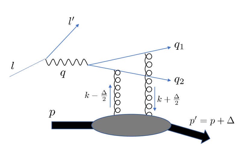
Figure 1: Exclusive dijet production in electron-proton scattering.

3 Double spin asymmetry in diffractive dijet production—We consider exclusive dijet production in electron-proton scattering depicted in Fig. 1. This process has attracted a lot of attention in the literature in different contexts Bartels:1996ne ; Braun:2005rg ; Altinoluk:2015dpi ; Hatta:2016dxp ; Boussarie:2016ogo ; Ji:2016jgn ; Hatta:2016aoc ; Hagiwara:2017fye ; Mantysaari:2019csc ; Salazar:2019ncp ; Boer:2021upt . However, longitudinal double spin asymmetry has not been studied to our knowledge. In the hadron frame, the longitudinally polarized proton moves fast in the $+x^{3}$ direction and the virtual photon with virtuality $q^{2}=-Q^{2}$ in the $-x^{3}$ direction. Two jets in the final state have longitudinal momentum fractions (of the photon) $z=p\cdot q_{1}/p\cdot q$ and $\bar{z}=1-z$, and transverse momenta $q_{\perp}-z\Delta_{\perp}$ and $-q_{\perp}-\bar{z}\Delta_{\perp}$, respectively, where $\Delta_{\perp}$ is the transverse momentum of the recoiling proton. $q_{\perp}$ is related to skewness $\xi$ and the $\gamma^{*}p$ center-of-mass energy $W^{2}=(p+q)^{2}$ as

$$\xi=\frac{q_{\perp}^{2}+z\bar{z}Q^{2}}{-q_{\perp}^{2}+z\bar{z}(Q^{2}+2W^{2})}.$$ (9)

The momenta of the incoming lepton is parameterized as $l^{\mu}=(l^{+},l^{-},l_{\perp})=(\frac{Q(1-y)}{\sqrt{2}y},\frac{Q}{\sqrt{2}y},\frac{Q\sqrt{1-y}}{y}n_{\perp})$ where $y=p\cdot q/p\cdot l$ as usual and $n_{\perp}=(\cos\phi_{l_{\perp}},\sin\phi_{l_{\perp}})$ is a unit vector in the transverse plane. The spin-dependent part of the lepton tensor is $L^{\mu\nu}\sim-2i\epsilon^{\mu\nu\rho\sigma}s_{\rho}q_{\sigma}$. For a longitudinally polarized lepton, $s_{\rho}=h_{l}l_{\rho}$ where $h_{l}=\pm 1$ is the helicity. In order to be sensitive to the azimuthal angle of the lepton plane $\phi_{l_{\perp}}$, the index $\rho$ has to be transverse. Since $\sigma=\pm$ is longitudinal, one of $\mu,\nu$ must be longitudinal and the other transverse. Namely, we should look at the interference effect between the longitudinal $A_{L}$ and transverse $A_{T}^{\lambda}$ $(\lambda=1,2$) virtual photon amplitudes

$$A_{L}=A_{L}^{2}+A_{L}^{3},\quad A^{\lambda}_{T}=\epsilon^{\lambda i}(A_{T}^{2i}+A_{T}^{3i}).$$ (10)

The twist-2 part $A^{2}_{L/T}$ is proportional to gluon GPDs and has been calculated in Braun:2005rg in the two-gluon exchange approximation (see Fig. 1). The twist-3 part $A^{3}_{L/T}$ involves GTMDs and retains one factor of $t$-channel gluon transverse momentum $k_{\perp}$. It has been calculated in Ji:2016jgn and here we reproduce the result

$$A^{3}_{T} =-\dfrac{ig^{2}_{s}e_{em}e_{q}}{N_{c}}\dfrac{2(\overline{z}-z)}{(q^{2}_{\perp}+\mu^{2})^{2}}\bar{u}(q_{1})\epsilon_{\perp}\cdot\gamma_{\perp}v(q_{2})$$

$$\quad\times\int dx\dfrac{x}{(x^{2}-\xi^{2}+i\xi\varepsilon)^{2}}\bigg{(}2\xi+\dfrac{(2\xi)^{3}(1-2\beta)}{(x^{2}-\xi^{2}+i\xi\varepsilon)}\bigg{)}$$

$$\quad\times\int d^{2}k_{\perp}q_{\perp}\cdot k_{\perp}\,xf_{g}(x,\xi,k_{\perp},\Delta_{\perp})$$

$$-\dfrac{ig^{2}_{s}e_{em}e_{q}}{N_{c}}\dfrac{2(2\xi)^{2}z\overline{z}W}{(q^{2}_{\perp}+\mu^{2})^{2}}\bar{u}(q_{1})\gamma^{-}v(q_{2})$$

$$\quad\times\int dx\dfrac{x}{(x^{2}-\xi^{2}+i\xi\varepsilon)^{2}}$$

$$\quad\times\int d^{2}k_{\perp}\epsilon_{\perp}\cdot k_{\perp}\,xf_{g}(x,\xi,k_{\perp},\Delta_{\perp}),$$ (11)

$$A^{3}_{L} =\dfrac{ig^{2}_{s}e_{em}e_{q}}{N_{c}}\dfrac{16\xi^{2}(\overline{z}-z)z\overline{z}QW}{(q^{2}_{\perp}+\mu^{2})^{3}}\bar{u}(q_{1})\gamma^{-}v(q_{2})$$

$$\quad\times\int dx\dfrac{x}{(x^{2}-\xi^{2}+i\xi\varepsilon)^{2}}\bigg{(}1+\dfrac{8\xi^{2}(1-\beta)}{(x^{2}-\xi^{2}+i\xi\varepsilon)}\bigg{)}$$

$$\quad\times\int d^{2}k_{\perp}\,q_{\perp}\cdot k_{\perp}\,xf_{g}(x,\xi,k_{\perp},\Delta_{\perp}),$$ (12)

where $\mu^{2}=z\bar{z}Q^{2}$ and $\beta=\frac{\mu^{2}}{q_{\perp}^{2}+\mu^{2}}$. The $k_{\perp}$-weighted integrals of $f_{g}$ lead to the moments (6) and (7). Importantly, in both the longitudinal and transverse amplitudes, the $x$-integral contains a third pole at $x=\pm\xi$. Such poles often imply the breakdown of collinear factorization due to diverging $x$-integrals Cui:2018jha . (Gluon GPDs may contain terms proportional to $\theta(\xi-x)(x^{2}-\xi^{2})^{2}$ which are not integrable if there is a third pole.) Fortunately, these potentially dangerous terms can be dropped by setting $z=1/2$, after which $A_{L}^{3}=0$ and only a second pole remains in $A_{T}^{3}$. Note that, if one considers SSA Ji:2016jgn , one cannot set $z=1/2$ because the asymmetry (2) vanishes at this point. After integrating over the jet azimuthal angle $\phi_{q_{\perp}}$, we obtain the following contribution to DSA at $z=1/2$

$$\dfrac{d\sigma}{dydQ^{2}d\phi_{l_{\perp}}dzdq_{\perp}^{2}d^{2}\Delta_{\perp}}$$

$$=\dfrac{\alpha_{em}y}{2^{11}\pi^{7}Q^{4}}\dfrac{\int d\phi_{q_{\perp}}L^{\mu\nu}A^{*}_{\mu}A_{\nu}}{(W^{2}+Q^{2})(W^{2}-M_{J}^{2})z\overline{z}},$$ (13)

where $M_{J}^{2}=q_{\perp}^{2}/(z\bar{z})=4q_{\perp}^{2}$ is the invariant mass of dijet and

$$\int d\phi_{q_{\perp}}L^{\mu\nu}A^{*}_{\mu}A_{\nu}$$

$$=-\dfrac{2^{10}\pi^{4}}{N_{c}}h_{l}h_{p}\alpha^{2}_{s}\alpha_{em}e^{2}_{q}\frac{(1+\xi)\xi Q^{2}}{(q_{\perp}^{2}+\mu^{2})^{2}}|l_{\perp}||\Delta_{\perp}|$$

$$\ \times\mathfrak{Re}\Bigg{[}\biggl{\{}{\cal H}^{(1)*}_{g}-\dfrac{\xi^{2}}{1-\xi^{2}}{\cal E}^{(1)*}_{g}$$

$$\qquad+\dfrac{4q^{2}_{\perp}}{q^{2}_{\perp}+\mu^{2}}\bigg{(}{\cal H}^{(2)*}_{g}-\dfrac{\xi^{2}}{1-\xi^{2}}{\cal E}^{(2)*}_{g}\bigg{)}\biggr{\}}{\cal L}_{g}$$

$$\quad+\left({\cal E}^{(1)*}_{g}+\dfrac{4q^{2}_{\perp}}{q^{2}_{\perp}+\mu^{2}}{\cal E}^{(2)*}_{g}\right)\frac{{\cal O}}{2}\Bigg{]}\textrm{cos}(\phi_{l_{\perp}}-\phi_{\Delta_{\perp}}).$$ (14)

The details of the calculation, including the case $z\neq 1/2$, will be presented elsewhere prep . The various ‘Compton form factors’ are defined as

$${\cal H}^{(1)}_{g}(\xi) = \int^{1}_{-1}dx\frac{H_{g}(x,\xi)}{(x-\xi+i\epsilon)(x+\xi-i\epsilon)},$$ (15)

$${\cal H}^{(2)}_{g}(\xi) = \int^{1}_{-1}dx\frac{\xi^{2}H_{g}(x,\xi)}{(x-\xi+i\epsilon)^{2}(x+\xi-i\epsilon)^{2}},$$ (16)

$${\cal L}_{g}(\xi) = \int^{1}_{-1}dx\frac{x^{2}L_{g}(x,\xi)}{(x-\xi+i\epsilon)^{2}(x+\xi-i\epsilon)^{2}},$$ (17)

$${\cal O}(\xi) = \int^{1}_{-1}dx\frac{xO(x,\xi)}{(x-\xi+i\epsilon)^{2}(x+\xi-i\epsilon)^{2}},$$ (18)

and ${\cal E}_{g}^{(1,2)}(\xi)$ is defined from $E_{g}(x,\xi)$ similarly to ${\cal H}_{g}^{(1,2)}(\xi)$. Assuming $|H_{g}|\gg|E_{g}|$, we see that the cross section is directly proportional to the Compton form factor of the gluon OAM ${\cal L}_{g}$. The characteristic correlation $k_{\perp}\times\Delta_{\perp}\sim\sin(\phi_{k_{\perp}}-\phi_{\Delta_{\perp}})$ of OAM manifests itself as a cosine correlation between the outgoing electron and proton angles. A similar transfer of angular correlations has been noticed in Zhou:2016rnt for the $\cos 2(\phi_{k_{\perp}}-\phi_{\Delta_{\perp}})$ dependence of the elliptic gluon GTMD Hatta:2016dxp ; Hagiwara:2021xkf . Away from the point $z=1/2$, there are corrections proportional to $(z-1/2)^{2}$, but collinear factorization is suspect for them as already mentioned. Instead, one should use the $k_{\perp}$-factorization approach to calculate the corrections, although their connection to the OAM is less clear.

4. DSA from the gluon helicity—Next we discuss another source of DSA from the gluon helicity GPDs

$$\epsilon_{ij}\int\frac{dz^{-}}{\pi}e^{ixP^{+}z^{-}}\langle p^{\prime}|F_{a}^{+i}(-z/2)F_{a}^{+j}(z/2)|p\rangle$$

$$=\bar{u}(p^{\prime})\left(i\tilde{H}_{g}\gamma_{5}\gamma^{+}-i\tilde{E}_{g}\frac{\gamma_{5}\Delta^{+}}{2M}\right)u(p),$$ (19)

where $\tilde{H}_{g}(x)=x\Delta G(x)$ in the forward limit. This originates from the interference between the unpolarized and polarized gluon GPDs in the amplitude and the complex-conjugate amplitude. An entirely analogous contribution should be added to the result for SSA in Ji:2016jgn ; Hatta:2016aoc . The $\cos(\phi_{l_{\perp}}-\phi_{\Delta_{\perp}})$ asymmetry due to this mechanism is actually known in the context of Deeply Virtual Compton Scattering (DVCS) Belitsky:2000gz . Unlike in DVCS, in dijet production there is no contamination from the Bethe-Heitler process. The asymmetry can be calculated purely within the GPD framework by setting $k_{\perp}=0$ but keeping one factor of $\Delta_{\perp}$ in the hard part. In general, the cross section contains integrals with a third pole such as

$$\int dx\frac{H_{g}(x,\xi)}{(x^{2}-\xi^{2}+i\xi\epsilon)^{3}},\quad\int dx\frac{x\tilde{H}_{g}(x,\xi)}{(x^{2}-\xi^{2}+i\xi\epsilon)^{3}}.$$ (20)

Remarkably, however, these factorization-breaking terms all vanish at $z=1/2$ and we find prep

$$\int d\phi_{q_{\perp}}L^{\mu\nu}A_{\mu}A_{\nu}=\frac{2^{10}\pi^{4}}{N_{c}}h_{l}h_{p}\alpha_{s}^{2}\alpha_{em}e_{q}^{2}\frac{(1-\xi^{2})\xi Q^{2}}{(q_{\perp}^{2}+\mu^{2})^{2}}$$

$$\quad\times\mathfrak{Re}\left[\left({\cal H}_{g}^{(1)*}-\frac{\xi^{2}}{1-\xi^{2}}{\cal E}_{g}^{(1)*}\right)\left(\tilde{\cal H}_{g}^{(2)}-\frac{\xi^{2}}{1-\xi^{2}}\tilde{\cal E}_{g}^{(2)}\right)\right]$$

$$\quad\times|l_{\perp}||\Delta_{\perp}|\cos(\phi_{l_{\perp}}-\phi_{\Delta_{\perp}}),$$ (21)

with

$$\tilde{\cal H}_{g}^{(2)}(\xi)=\int dx\frac{x\tilde{H}_{g}(x,\xi)}{(x^{2}-\xi^{2}+i\xi\epsilon)^{2}},$$

$$\tilde{\cal E}_{g}^{(2)}(\xi)=\int dx\frac{x\tilde{E}_{g}(x,\xi)}{(x^{2}-\xi^{2}+i\xi\epsilon)^{2}}.$$ (22)

In the following, we shall be mainly interested in the small-$\xi$ region $\xi\lesssim 10^{-3}$. In this region ${\cal H}_{g}^{(1,2)}(\xi)$ are dominated by the imaginary part, and one can show that $\mathfrak{Im}{\cal H}_{g}^{(1)}\approx-2\mathfrak{Im}{\cal H}_{g}^{(2)}$. Combining (21) with (14) and neglecting ${\cal E}_{g}$ and $\tilde{\cal E}_{g}$, we find that the asymmetry is roughly proportional to the combination

$${\cal H}^{(1)*}_{g}\left(\tilde{\cal H}_{g}^{(2)}+\frac{q_{\perp}^{2}-\mu^{2}}{q_{\perp}^{2}+\mu^{2}}{\cal L}_{g}\right).$$ (23)

Depending on the sign of $q_{\perp}^{2}-\mu^{2}=q_{\perp}^{2}-Q^{2}/4$, the helicity and OAM contributions interfere positively or negatively. Note that $\tilde{\cal H}_{g}^{(2)}\pm{\cal L}_{g}\sim\Delta G(x)\pm L_{g}(x)$, and $\Delta G(x)\approx-L_{g}(x)$ at small-$x$ Hatta:2016aoc ; Hatta:2018itc ; More:2017zqp ; Boussarie:2019icw (see however, Kovchegov:2019rrz ). Thus, the two contributions have the same sign when $q_{\perp}^{2}<Q^{2}/4$ but tend to cancel each other when $q_{\perp}^{2}>Q^{2}/4$. By varying $Q^{2}$, we should be able to see this very interesting interplay between the helicity and the OAM.

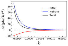
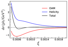
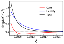
Figure 2: The DSA part of the differential cross section (25) at $Q^{2}=2.7$ GeV² (left), $Q^{2}=4.8$ GeV² (middle) and $Q^{2}=10$ GeV² (right). The labels ‘OAM’ and ‘Helicity’ refer to the two contributions (14) and (21), respectively.

5. Numerical results—We now present a numerical estimate of the cross section. We neglect $E_{g},\tilde{E}_{g}$ altogether. $H_{g}(x,\xi)$, $\tilde{H}_{g}(x,\xi)$ and $xL_{g}(x,\xi)$ are reconstructed from their PDF counterparts $xG(x)$, $x\Delta G(x)$ and $xL_{g}(x)$, respectively, using the method of double distributions Radyushkin:1998es ; Radyushkin:2000uy . We use the JAM Sato:2019yez ; Ethier:2017zbq gluon PDFs $xG(x)$ and $x\Delta G(x)$ as inputs. As for $xL_{g}(x)$, we employ the Wandzura-Wilczek (WW) approximation Hatta:2012cs

$$L_{g}(x)\approx x\int^{1}_{x}\frac{dx^{\prime}}{x^{\prime 2}}x^{\prime}G(x^{\prime})-2x\int_{x}^{1}\frac{dx^{\prime}}{x^{\prime 2}}\Delta G(x^{\prime}),$$ (24)

although we are eventually interested in constraining the genuine twist-three part neglected in this approximation. We integrate over $\Delta_{\perp}$ assuming a Gaussian form factor $e^{-b\Delta_{\perp}^{2}}$ with $b=5$ GeV^-2 Braun:2005rg and change variables $q_{\perp}\to\xi$ according to (9). The other parameters are fixed as $h_{p}h_{l}=1$, $\sqrt{s_{ep}}=120$ GeV and $y=0.7$. The resulting cross section (only the DSA part)

$$\frac{d\sigma}{dydQ^{2}dzd\xi d\delta\phi},$$ (25)

is shown in Fig. 2 at $\delta\phi=\phi_{l_{\perp}}-\phi_{\Delta_{\perp}}=0$ for three different values of $Q^{2}$ (2.7 GeV², 4.8 GeV² and 10 GeV²). The plots correspond to $1<q_{\perp}<3$ GeV ($1<q_{\perp}<2.35$ GeV in the $Q^{2}=2.7$ GeV² case). Typical jet rapidities in the laboratory frame are $-2<\eta<-1$ at the top EIC energy $E_{p}\sim 250$ GeV. We see that the OAM (14) and helicity (21) contributions are comparable in magnitude, though the latter tends to be larger because of the cancellation between ${\cal H}^{(1)}_{g}$ and ${\cal H}_{g}^{(2)}$. As a result of this cancellation, we observe a clear sign change of the OAM contribution with increasing $Q^{2}$, see (23). It should be mentioned that there are large uncertainties in our prediction even in the helicity part because currently $\Delta G(x)$ is poorly constrained, including even the sign, especially in the small-$x$ region but also in the large-$x$ region. (See a recent discussion Zhou:2022wzm on this point.) Besides, nothing is known about $L_{g}(x)$ experimentally at the moment, and our model for ${\cal L}_{g}$ involves key assumptions (the WW approximation and the use of the double distribution technique) whose validity needs to be investigated. The above result should thus be regarded as an exploratory study to be significantly improved in future. Nonetheless, our calculation adequately demonstrates the feasibility of accessing the OAM from DSA. Ultimately, ${\cal L}_{g}$ can be extracted from future experimental data, and for this purpose an accurate determination of $xG(x)$ and $x\Delta G(x)$ down to $x\sim 10^{-3}$ is crucial.

6. Conclusions—We have proposed DSA in exclusive dijet production as a novel observable for the gluon OAM $L_{g}$ that can be measured at the EIC. Compared to SSA (2) previously suggested in Ji:2016jgn ; Hatta:2016aoc , it has a number of advantages. Most importantly, the third poles at $x=\pm\xi$ in (11), (12) and (20) which are potentially dangerous for QCD factorization can be eliminated by setting $z=1/2$, but this is not possible in SSA. In practice, measurements are done in some window in $z$. We expect that the cross section $d\sigma/dz$ varies mildly around $z\sim 1/2$, but this needs to be substantiated in future investigations. Second, unlike the jet angle $\phi_{q_{\perp}}$, the electron angle $\phi_{l_{\perp}}$ is not affected by final state QCD radiations. The former is integrated over in DSA, and this greatly simplifies the cross section formula without losing sensitivity to the OAM. We thus expect that DSA is more robust against higher order QCD corrections to this process Boussarie:2016ogo . Furthermore, in the limit $x\approx\xi\to 0$, ${\cal H}_{g}^{(1,2)}$ are dominantly imaginary, and the extraction of the imaginary part in (2) turned out to be a delicate problem within the effective theory of high energy QCD Hatta:2016aoc . For DSA, such a concern is simply absent. (We however note that in the present GPD-like approach, the real and imaginary parts of ${\cal L}_{g}$ are comparable in magnitude.)

The present calculation can be straightforwardly extended to the quark exchange channel important in the low-energy (low-$W$, high-$\xi$) region. We expect an additional contribution proportional to the product of the quark GPD and the quark OAM $\sim{\cal H}^{*}_{q}{\cal L}_{q}$. This will be a nice addition to the finding in Bhattacharya:2017bvs which is so far the only observable known to be sensitive to $L_{q}$.

Acknowledgements—We thank Feng Yuan and Yong Zhao for explaining to us the results in Ji:2016jgn and for discussion. S. B. and Y. H. were supported by the U.S. Department of Energy under Contract No. DE-SC0012704, and also by Laboratory Directed Research and Development (LDRD) funds from Brookhaven Science Associates. S. B. has also been supported by the U.S. Department of Energy, Office of Science, Office of Nuclear Physics and Office of Advanced Scientific Computing Research within the framework of Scientific Discovery through Advance Computing (SciDAC) award Computing the Properties of Matter with Leadership Computing Resources.

References

(1)
L. Adamczyk et al. [STAR],
Phys. Rev. Lett. 115 (2015), 092002
[arXiv:1405.5134 [hep-ex]].
(2)
D. de Florian, R. Sassot, M. Stratmann and W. Vogelsang,
Phys. Rev. Lett. 113 (2014), 012001
[arXiv:1404.4293 [hep-ph]].
(3)
E. R. Nocera et al. [NNPDF],
Nucl. Phys. B 887 (2014), 276-308
[arXiv:1406.5539 [hep-ph]].
(4)
J. J. Ethier, N. Sato and W. Melnitchouk,
Phys. Rev. Lett. 119 (2017), 132001
[arXiv:1705.05889 [hep-ph]].
(5)
M. S. Abdallah et al. [STAR],
[arXiv:2110.11020 [hep-ex]].
(6)
R. Abdul Khalek, A. Accardi, J. Adam, D. Adamiak, W. Akers, M. Albaladejo, A. Al-bataineh, M. G. Alexeev, F. Ameli and P. Antonioli, et al.
[arXiv:2103.05419 [physics.ins-det]].
(7)
R. Boussarie, Y. Hatta and F. Yuan,
Phys. Lett. B 797 (2019), 134817
[arXiv:1904.02693 [hep-ph]].
(8)
Y. V. Kovchegov,
JHEP 03 (2019), 174
[arXiv:1901.07453 [hep-ph]].
(9)
M. Engelhardt, J. R. Green, N. Hasan, S. Krieg, S. Meinel, J. Negele, A. Pochinsky and S. Syritsyn,
Phys. Rev. D 102 (2020), 074505
[arXiv:2008.03660 [hep-lat]].
(10)
Y. Guo, X. Ji and K. Shiells,
Nucl. Phys. B 969 (2021), 115440
[arXiv:2101.05243 [hep-ph]].
(11)
X. Ji, F. Yuan and Y. Zhao,
Phys. Rev. Lett. 118 (2017), 192004
[arXiv:1612.02438 [hep-ph]].
(12)
Y. Hatta, Y. Nakagawa, F. Yuan, Y. Zhao and B. Xiao,
Phys. Rev. D 95 (2017), 114032
[arXiv:1612.02445 [hep-ph]].
(13)
S. Bhattacharya, A. Metz and J. Zhou,
Phys. Lett. B 771 (2017), 396-400
[erratum: Phys. Lett. B 810 (2020), 135866]
[arXiv:1702.04387 [hep-ph]].
(14)
S. Bhattacharya, A. Metz, V. K. Ojha, J. Y. Tsai and J. Zhou,
[arXiv:1802.10550 [hep-ph]].
(15)
A. Courtoy, G. R. Goldstein, J. O. Gonzalez Hernandez, S. Liuti and A. Rajan,
Phys. Lett. B 731 (2014), 141-147
[arXiv:1310.5157 [hep-ph]].
(16)
C. Lorce and B. Pasquini,
Phys. Rev. D 84 (2011), 014015
[arXiv:1106.0139 [hep-ph]].
(17)
Y. Hatta,
Phys. Lett. B 708 (2012), 186-190
[arXiv:1111.3547 [hep-ph]].
(18)
C. Lorce, B. Pasquini, X. Xiong and F. Yuan,
Phys. Rev. D 85 (2012), 114006
[arXiv:1111.4827 [hep-ph]].
(19)
A. V. Belitsky, X. d. Ji and F. Yuan,
Phys. Rev. D 69 (2004), 074014
[arXiv:hep-ph/0307383 [hep-ph]].
(20)
S. Meissner, A. Metz and M. Schlegel,
JHEP 08 (2009), 056
[arXiv:0906.5323 [hep-ph]].
(21)
C. Lorcé and B. Pasquini,
JHEP 09 (2013), 138
[arXiv:1307.4497 [hep-ph]].
(22)
Y. Hatta and S. Yoshida,
JHEP 10 (2012), 080
[arXiv:1207.5332 [hep-ph]].
(23)
J. Zhou,
Phys. Rev. D 89 (2014), 074050
[arXiv:1308.5912 [hep-ph]].
(24)
J. Bartels, H. Lotter and M. Wüsthoff,
Phys. Lett. B 379 (1996), 239-248
[erratum: Phys. Lett. B 382 (1996), 449-449]
[arXiv:hep-ph/9602363 [hep-ph]].
(25)
V. M. Braun and D. Y. Ivanov,
Phys. Rev. D 72 (2005), 034016
[arXiv:hep-ph/0505263 [hep-ph]].
(26)
T. Altinoluk, N. Armesto, G. Beuf and A. H. Rezaeian,
Phys. Lett. B 758 (2016), 373-383
[arXiv:1511.07452 [hep-ph]].
(27)
Y. Hatta, B. W. Xiao and F. Yuan,
Phys. Rev. Lett. 116 (2016), 202301
[arXiv:1601.01585 [hep-ph]].
(28)
R. Boussarie, A. V. Grabovsky, L. Szymanowski and S. Wallon,
JHEP 11 (2016), 149
[arXiv:1606.00419 [hep-ph]].
(29)
Y. Hagiwara, Y. Hatta, R. Pasechnik, M. Tasevsky and O. Teryaev,
Phys. Rev. D 96 (2017), 034009
[arXiv:1706.01765 [hep-ph]].
(30)
H. Mäntysaari, N. Mueller and B. Schenke,
Phys. Rev. D 99 (2019), 074004
[arXiv:1902.05087 [hep-ph]].
(31)
F. Salazar and B. Schenke,
Phys. Rev. D 100 (2019), 034007
[arXiv:1905.03763 [hep-ph]].
(32)
D. Boer and C. Setyadi,
Phys. Rev. D 104 (2021), 074006
[arXiv:2106.15148 [hep-ph]].
(33)
Z. L. Cui, M. C. Hu and J. P. Ma,
Eur. Phys. J. C 79 (2019), 812
[arXiv:1804.05293 [hep-ph]].
(34)
S. Bhattacharya, R. Boussarie and Y. Hatta, work in progress.
(35)
J. Zhou,
Phys. Rev. D 94 (2016), 114017
[arXiv:1611.02397 [hep-ph]].
(36)
Y. Hagiwara, C. Zhang, J. Zhou and Y. j. Zhou,
Phys. Rev. D 104 (2021), 094021.
(37)
A. V. Belitsky, D. Mueller, L. Niedermeier and A. Schafer,
Nucl. Phys. B 593 (2001), 289-310
[arXiv:hep-ph/0004059 [hep-ph]].
(38)
Y. Hatta and D. J. Yang,
Phys. Lett. B 781 (2018), 213-219
[arXiv:1802.02716 [hep-ph]].
(39)
J. More, A. Mukherjee and S. Nair,
Eur. Phys. J. C 78 (2018), 389
[arXiv:1709.00943 [hep-ph]].
(40)
A. V. Radyushkin,
Phys. Rev. D 59 (1999), 014030
[arXiv:hep-ph/9805342 [hep-ph]].
(41)
A. V. Radyushkin,
[arXiv:hep-ph/0101225 [hep-ph]].
(42)
N. Sato et al. [JAM],
Phys. Rev. D 101 (2020), 074020
[arXiv:1905.03788 [hep-ph]].
(43)
Y. Zhou, N. Sato and W. Melnitchouk,
[arXiv:2201.02075 [hep-ph]].