Energetic bounds on gyrokinetic instabilities. Part II. Modes of optimal growth.

Abstract

We introduce modes of instantaneous optimal growth of free energy for the fully electromagnetic gyrokinetic equations. We demonstrate how these “optimal modes” arise naturally from the free energy balance equation, allowing its convenient decomposition, and yielding a simple picture of energy flows. Optimal modes have a number of other favorable features, such as their low-dimensionality, efficiency of computation, and the fact that their growth rates provide a rigorous and “tight” upper bound on both the nonlinear growth rate of energy, and the linear growth rate of traditional gyrokinetic (normal mode) instabilities. We provide simple closed form solutions for the optimal growth rates in a number of asymptotic limits, and compare these with our previous bounds.

1 Introduction

This is the second paper in a series, in which we develop a linear and nonlinear stability theory based on gyrokinetic energy balance. Whereas the first paper emphasizes simple and rigorous upper bounds, this second paper shifts focus to tightening these bounds (making them exactly realizable under the right initial conditions), fully generalizing their validity (allowing fully electromagnetic fluctuations including non-zero $\delta B_{\parallel}$), and introducing the notion of a complete orthogonal set of “optimal modes” associated with these bounds.

Gyrokinetic stability analysis serves as the foundation of turbulence and transport theory for magnetic fusion devices, with linear calculations being the starting point for predicting turbulence intensity and other properties. Such calculations are also the main ingredient of mixing-length estimates (horton-rev), quasi-linear theory (Bourdelle_2015), and other (indeed, perhaps all) transport models. These linear instabilities are typically understood (with some notable exceptions, e.g. Hatch_2016) as “normal modes”, i.e. eigenmodes of the linearized gyrokinetic equation, whose time dependence takes the form $\sim\exp(-i\omega t)$, where $\Imag[\omega]=\gamma_{\mathrm{L}}$ is the growth rate. When numerically computing gyrokinetic normal modes, it is most common to solve an initial value problem, and terminate the computation only when the solution is found to fit the exponential form. This technique yields the mode of largest growth rate for a given wave number.

This paper introduces a different kind of gyrokinetic mode, one that realizes optimal growth of energy at an instant in time (actually, the idea was proposed first in the gyrokinetic context by landreman_plunk_dorland_2015 but not calculated explicitly there). These modes have been studied extensively in fluid turbulence, where they are called “instantaneous optimal perturbations”, and are found as a limit of a more general class of modes that achieve optimal growth of energy over a finite time interval (farrell-generalized-stability-theory).

To illustrate the essential idea of such modes, free from the complications of full gyrokinetics, let us consider a simple schematic equation for a linearized dynamical system with a complex state variable $\psi(t,\ell)$, where $t$ is time and $\ell$ is a continuous space variable,

$$\frac{\partial\psi}{\partial t}=\cal{L}\psi,$$ (1)

with $\cal{L}$ representing some linear operator, whose eigenmodes are precisely the “normal modes” described above. Defining an inner product (involving, e.g., a suitable average over $\ell$), we obtain an “energy” evolution equation for $\left(\psi,\psi\right)=||\psi||^{2}$

$$\frac{d||\psi||^{2}}{dt}=\left(\psi,{\cal H}\psi\right),$$ (2)

where ${\cal H}=\cal{L}+\cal{L}^{\dagger}$ is a Hermitian linear operator, with the adjoint operator $\cal{L}^{\dagger}$ defined as that for which $\left(\psi_{1},{\cal L}\psi_{2}\right)=\left({\cal L}^{\dagger}\psi_{1},\psi_{2}\right)$ holds for arbitrary $\psi_{1}$ and $\psi_{2}$ in the Hilbert space defined by the inner product. From this we can immediately surmise that the eigenmodes of ${\cal H}$, i.e. $\psi_{n}$ such that ${\cal H}\psi_{n}=\lambda_{n}\psi_{n}$, can be used to characterize the energy growth of the system, as their orthogonality reduces the right hand side of this equation to the sum of the squares of eigenmode amplitudes, times their eigenvalues. These are precisely the “optimal modes” described above. Writing $\psi=\sum_{n}c_{n}\psi_{n}$, and taking $||\psi_{n}||^{2}=1$, we have

$$\sum_{n}\frac{d|c_{n}|^{2}}{dt}=\sum_{n}\lambda_{n}|c_{n}|^{2}.$$ (3)

Obviously, the eigenmode with the largest positive value achieves optimal growth, i.e. maximizes $||\psi||^{-2}d||\psi||^{2}/dt$.

Note that “instantaneous optimal perturbations” achieve optimal growth only for an instant. That is, if the system is initialized to be an optimal solution, the observed growth of energy will generally only match the theoretical value initially, and the solution, left undisturbed by nonlinear physics, will evolve over a certain timescale toward a normal mode described above. Clearly, if this timescale is much longer than the nonlinear decorrelation rate of the turbulence, then the growth of normal modes cannot be expected to be a useful measure, and an alternative measure, such as the optimal rate, may be better. Furthermore, there are cases where turbulence arises when no unstable normal modes exist at all, this being the original motivation for introducing optimal modes. For so-called “sub-critical” turbulence, one needs a measure to characterize the transient linear growth of fluctuations. It is not difficult to see that modes of positive instantaneous optimal growth, one such measure, are necessary for sub-critical turbulence to exist (del-sole_necessity). Indeed, from Eqn. 3, the energy of the system can only ever increase if eigenmodes exist with $\lambda_{n}>0$.

Even in cases where growth rate of normal modes is found to be a suitable measure of instability, we note that the analysis of optimal modes provides a rigorous upper bound to that growth: if $\gamma$ is an eigenvalue of ${\cal L}$ in the system above, then $\gamma\leq\max_{n}\lambda_{n}/2$.

For gyrokinetics, we can point to several further advantages of optimal modes. The first, as we will see, is the drastic reduction in the dimensionality of the problem, as compared to normal mode analysis, for which the kinetic distribution of each particle species requires two velocity variables to be accounted for, in addition to time and space. The complete analysis of optimal modes, in contrast, requires only a few velocity moments to be computed, eliminating the vast majority of the complexity of velocity space. Explicit time evolution, required in initial value computations, is also avoided, and the modes we find are “local” in position space, i.e. the field-line following coordinate becomes merely a parameter of the theory. Furthermore, the singular nature of modes in kinetic theory (e.g. Case-Van Kampen modes, etc.) is evaded, and the optimal modes form a complete and orthogonal basis for the entire space of gyrokinetic fluctuations. This gives a natural way to decompose energy balance (see Eqn. 3), and simplifies the analysis of energy flows in the turbulent steady state – the turbulence is excited by unstable modes (with $\lambda_{n}>0$) and damped by stable ones (with $\lambda_{n}<0$). Optimal mode theory, following directly from energy balance, gives a universal bound on the full “zoo” of gyrokinetic instabilities, in contrast to traditional linear (normal) mode analysis, which requires detailed, separate analysis of different cases. Optimal modes therefore give a unified picture of the space of instabilities.

As we will see, many useful cases of optimal growth can be evaluated with simple closed-form expressions, without the need for numerical computation; when such computation is needed, its cost is trivial. In short, we will show that optimal modes can be viewed as a theoretically transparent and computationally efficient alternative (or complement) to normal modes in gyrokinetics.

2 Definitions and gyrokinetic free energy balance

We are interested in finding the solutions that optimize the growth of a certain measure of fluctuation energy. The choice that we have made so far in this series of articles is the gyrokinetic Helmholtz free energy, commonly referred to as simply “free energy”. This measure has the advantage of being a “nonlinear invariant”, i.e. conserved under nonlinear interactions, and also having a satisfying thermodynamic interpretation – it only diminishes under the action of collisions. These facts are well known and spelled out in part I of this series. We can therefore begin directly with the energy balance equation, which, neglecting collisions, reads

$$\frac{d}{dt}\sum_{\bf k}H=2\sum_{\bf k}D,$$ (4)

where the perpendicular wavenumber is ${\bf k}={\bf k}_{\perp}=k_{\psi}\bnabla\psi+k_{\alpha}\bnabla\alpha$, in terms of magnetic coordinates $\psi$ and $\alpha$ such that the equilibrium magnetic field is ${\bf B}=\bnabla\psi\times\bnabla\alpha$. The drive term $D$ is

$$D({\bf k},t)={\rm Im}\;\sum_{a}e_{a}\left\langle\int g_{a,\bf k}\omega_{\ast a}^{T}\bar{\chi}^{\ast}_{a,\bf k}d^{3}v\right\rangle,$$ (5)

and the free energy is

$$H({\bf k},t)=\sum_{a}\left\langle T_{a}\int\frac{|g_{a,\bf k}|^{2}}{F_{a0}}d^{3}v-\frac{n_{a}e_{a}^{2}}{T_{a}}|\delta\phi_{\bf k}|^{2}\right\rangle+\left\langle\frac{|\delta{\bf B}_{\bf k}|^{2}}{\mu_{0}}\right\rangle,$$ (6)

where $|\delta{\bf B}_{\bf k}|^{2}=|k_{\perp}\delta A_{\|\bf k}|^{2}+|\delta B_{\|\bf k}|^{2}$, and we define the other notation as follows. The space average is defined as

$$\left\langle\cdots\right\rangle=\lim_{L\rightarrow\infty}\int_{-L}^{L}(\cdots)\frac{dl}{B}\bigg{/}\int_{-L}^{L}\frac{dl}{B}.$$ (7)

The diamagnetic frequencies are

$$\omega_{\ast a}=\frac{k_{\alpha}T_{a}}{e_{a}}\frac{d\ln n_{a}}{d\psi},$$

$$\omega_{\ast a}^{T}=\omega_{\ast a}\left[1+\eta_{a}\left(\frac{m_{a}v^{2}}{2T_{a}}-\frac{3}{2}\right)\right].$$

The gyro-averaged electromagnetic potential is

$$\bar{\chi}_{a\bf k}=J_{0}\left(\frac{k_{\perp}v_{\perp}}{\Omega_{a}}\right)\left(\delta\phi_{{\bf k}}-v_{\|}\delta A_{\|{\bf k}}\right)+J_{1}\left(\frac{k_{\perp}v_{\perp}}{\Omega_{a}}\right)\frac{v_{\perp}}{k_{\perp}}\delta B_{\|\bf k},$$

and $J_{0}$ and $J_{1}$ are Bessel functions. Field perturbations are given by

$$\sum_{a}\frac{n_{a}e_{a}^{2}}{T_{a}}\;\delta\phi_{\bf k}=\sum_{a}e_{a}\int g_{a,{\bf k}}J_{0a}d^{3}v,$$ (8)

$$\delta A_{\|{\bf k}}=\frac{\mu_{0}}{k_{\perp}^{2}}\sum_{a}e_{a}\int v_{\|}g_{a,{\bf k}}J_{0a}d^{3}v,$$ (9)

$$\delta B_{\|{\bf k}}=-\frac{\mu_{0}}{k_{\perp}}\sum_{a}e_{a}\int v_{\perp}g_{a,{\bf k}}J_{1a}d^{3}v,$$ (10)

where we define $J_{na}=J_{n}(k_{\perp}v_{\perp}/\Omega_{a})$. Henceforth consider a single fixed value of $\bf k$ and therefore suppress the $\bf k$-subscripts.

Note that we define the free energy as twice that which appears in some other publications, but this has no significant effect on the analysis, as the 2 drops out of the optimization problem, upon division by $H$.

3 Modes of optimal instantaneous growth

To recast Eqn. 4 in the form of Eqn. 2 requires first identifying the state variable(s) and inner product. We take the state to be the set of distributions functions, given by the vector ${\bf g}$ with components $g_{a}$, and define the inner product of two states ${\bf g}_{1}$ and ${\bf g}_{2}$ as

$$({\bf g}_{1},{\bf g}_{2})=\sum_{a}\left\langle T_{a}\int\frac{g_{a1}^{*}g_{a2}}{F_{a0}}d^{3}v\right\rangle.$$ (11)

Comparing with Eqn. 6, we note that the free energy $H$ is not the Euclidean norm in these variables (though it is positive-definite in ${\bf g}$ for non-zero wavenumber; see helander-plunk-jpp-part-1). Although it is possible to transform to new state variables, i.e. $\tilde{\bf g}$ such that $H=||\tilde{{\bf g}}||^{2}$, we find it is more convenient to take another approach at this stage, namely to formulate our problem in variational terms. That is, we extremize the ratio

$$\Lambda=D/H$$ (12)

over the space of distribution functions ${\bf g}$. Note also that, as is easily verified, normal modes satisfy $\gamma_{L}=D/H$, so that we have the bound on linear gyrokinetic instabilities:

$$\gamma_{L}\leq\max_{g_{a}}\Lambda.$$ (13)

Variation of Eqn. 12 leads to the condition

$$\frac{\delta D}{\delta g_{a}}-\Lambda\frac{\delta H}{\delta g_{a}}=0.$$ (14)

Note that $\Lambda$, which according to Eqn. 4 corresponds to half the growth rate of free energy, can be interpreted as the Lagrange multiplier whose role is to hold $H$ fixed.

Using Eqns. 5 and 6, we can evaluate Eqn. 14 to obtain (see Appendix A)

$$\Lambda\sum_{b}{\cal H}_{ab}g_{b}=\sum_{b}{\cal D}_{ab}g_{b},$$ (15)

where ${\cal H}$ and ${\cal D}$ are, respectively, a purely real and purely imaginary Hermitian linear operators on the space of distribution functions, given as follows:

$${\cal H}_{ab}g_{b}=\delta_{a,b}g_{b}+\frac{F_{a0}}{n_{a}T_{a}}\frac{1}{n_{b}}\int d^{3}v^{\prime}g_{b}^{\prime}\left[-t_{a}t_{b}\psi_{1a}\psi_{1b}^{\prime}+\varepsilon_{a}\varepsilon_{b}(\psi_{3a}\psi_{3b}^{\prime}+\psi_{5a}\psi_{5b}^{\prime})\right],$$ (16)

noting that the species label $b$ is not to be confused with the argument of the Bessel functions, and $\delta_{a,b}$ is the discrete delta function. The second operator is given by

$${\cal D}_{ab}g_{b}= \frac{i}{2}\frac{F_{a0}}{n_{a}T_{a}}\frac{1}{n_{b}}\int d^{3}v^{\prime}g_{b}^{\prime}\left[\right.$$

$$\omega_{\ast a}\left(1-3\eta_{a}/2\right)\left(t_{a}t_{b}\psi_{1a}\psi_{1b}^{\prime}-\varepsilon_{a}\varepsilon_{b}\psi_{3a}\psi_{3b}^{\prime}-\varepsilon_{a}\varepsilon_{b}\psi_{5a}\psi_{5b}^{\prime}\right)$$

$$- \omega_{\ast b}\left(1-3\eta_{b}/2\right)\left(t_{a}t_{b}\psi_{1a}\psi_{1b}^{\prime}-\varepsilon_{a}\varepsilon_{b}\psi_{3a}\psi_{3b}^{\prime}-\varepsilon_{a}\varepsilon_{b}\psi_{5a}\psi_{5b}^{\prime}\right)$$

$$+ \omega_{\ast a}\eta_{a}\left(t_{a}t_{b}\psi_{2a}\psi_{1b}^{\prime}-\varepsilon_{a}\varepsilon_{b}\psi_{4a}\psi_{3b}^{\prime}-\varepsilon_{a}\varepsilon_{b}\psi_{6a}\psi_{5b}^{\prime}\right)$$

$$- \omega_{\ast b}\eta_{b}\left(t_{a}t_{b}\psi_{1a}\psi_{2b}^{\prime}-\varepsilon_{a}\varepsilon_{b}\psi_{3a}\psi_{4b}^{\prime}-\varepsilon_{a}\varepsilon_{b}\psi_{5a}\psi_{6b}^{\prime}\right)\left.\right],$$ (17)

where primes denote evaluation at $v^{\prime}$, and we define

$$t_{a} = e_{a}n_{a}\left(\sum_{a^{\prime}}\frac{n_{a^{\prime}}e_{a^{\prime}}^{2}}{T_{a^{\prime}}}\right)^{-1/2},$$ (18)

$$\varepsilon_{a} = e_{a}n_{a}\left(\frac{\sqrt{\mu_{0}}v_{Ta}}{k_{\perp}}\right)=\mathrm{sgn}(e_{a})\sqrt{n_{a}T_{a}\beta_{a}/b_{a}},$$ (19)

where $\mathrm{sgn}(e_{a})=\pm 1$ gives the sign of $e_{a}$, $b_{a}=k_{\perp}^{2}m_{a}T_{a}/(e_{a}^{2}B^{2})$, the plasma beta of species $a$ is $\beta_{a}=2\mu_{0}n_{a}T_{a}/B^{2}$, and its thermal velocity is denoted $v_{Ta}=\sqrt{2T_{a}/m_{a}}$. We also introduce velocity dependent functions that are needed for forming the relevant moments

$$\psi_{1a}=J_{0a},$$

(20)

3.1 Moment form of Eqn. 15

Eqn. 15 describes an eigenproblem whose solutions form a complete orthogonal basis for the space of distribution functions $g_{a}$. This is a large space, but as we will see, the non-trivial solution space of 15 is actually quite small. There are a number of reasons for this, but the first and most important is that only a small set of velocity moments appear in this equation. We can identify six dimensionless moments for each species, defined as

$$\kappa_{na}=\frac{1}{n_{a}}\int d^{3}v\;\psi_{na}g_{a}.$$ (21)

We further note that, due to the summation over species involved in the computation of the electromagnetic fields and free energy balance, the velocity moments $\kappa_{n}$ appear in particular linear combinations. Thus there is an additional dimensional reduction corresponding to the number of species $N_{s}$, i.e. $6N_{s}\rightarrow 6$. This is achieved with the help of the following barred variables

$$\bar{\kappa}_{1}=\sum_{a}t_{a}\kappa_{1a}$$, ,

, ,

, ,

(22)

where we introduce the normalized frequency $\bar{\omega}_{\ast a}=\omega_{\ast a}/\omega_{\ast}$, with $\omega_{\ast}$ an arbitrary reference value. Evaluating the sum over species in Equation 15 yields

$$\frac{\Lambda}{\omega_{*}}\left(g_{a}+\frac{F_{a0}}{n_{a}T_{a}}\left[-t_{a}\psi_{1a}\bar{\kappa}_{1}+\varepsilon_{a}(\psi_{3a}\bar{\kappa}_{3}+\psi_{5a}\bar{\kappa}_{5})\right]\right)\\ =\frac{i}{2}\frac{F_{a0}}{n_{a}T_{a}}\left[\right.\bar{\omega}_{\ast a}\left(1-3\eta_{a}/2\right)\left(t_{a}\psi_{1a}\bar{\kappa}_{1}-\varepsilon_{a}\psi_{3a}\bar{\kappa}_{3}-\varepsilon_{a}\psi_{5a}\bar{\kappa}_{5}\right)\\ +\bar{\omega}_{\ast a}\eta_{a}\left(t_{a}\psi_{2a}\bar{\kappa}_{1}-\varepsilon_{a}\psi_{4a}\bar{\kappa}_{3}-\varepsilon_{a}\psi_{6a}\bar{\kappa}_{5}\right)\\ -t_{a}\psi_{1a}\bar{\kappa}_{2}+\varepsilon_{a}\psi_{3a}\bar{\kappa}_{4}+\varepsilon_{a}\psi_{5a}\bar{\kappa}_{6}\left.\right].$$ (23)

To simplify the problem further, we can take moments of Equation 23 and obtain a closed linear system for $\bar{\kappa}_{n}$. We first write Equation 22 as

$$\bar{\kappa}_{m}=\sum_{n,b}c_{mn}^{(b)}\kappa_{nb}.$$ (24)

Now taking moments of 23, and summing over species, using Equation 24, we obtain

$$\frac{\Lambda}{\omega_{\ast}}\left(\bar{\kappa}_{m}+\sum_{a,n}\left\{-{\mathcal{T}}_{mn}^{(a)}X_{1n}^{(a)}\bar{\kappa}_{1}+{\mathcal{E}}_{mn}^{(a)}(X_{3n}^{(a)}\bar{\kappa}_{3}+X_{5n}^{(a)}\bar{\kappa}_{5})\right\}\right)\\ =\sum_{a,n}\frac{i}{2}\left\{\bar{\omega}_{\ast a}\left(1-3\eta_{a}/2\right)\left[{\mathcal{T}}_{mn}^{(a)}X_{1n}^{(a)}\bar{\kappa}_{1}-{\mathcal{E}}_{mn}^{(a)}\left(X_{3n}^{(a)}\bar{\kappa}_{3}+X_{5n}^{(a)}\bar{\kappa}_{5}\right)\right]\right.\\ +\bar{\omega}_{\ast a}\eta_{a}\left[{\mathcal{T}}_{mn}^{(a)}X_{2n}^{(a)}\bar{\kappa}_{1}-{\mathcal{E}}_{mn}^{(a)}\left(X_{4n}^{(a)}\bar{\kappa}_{3}+X_{6n}^{(a)}\bar{\kappa}_{5}\right)\right]\\ \left.-{\mathcal{T}}_{mn}^{(a)}X_{1n}^{(a)}\bar{\kappa}_{2}+{\mathcal{E}}_{mn}^{(a)}\left(X_{3n}^{(a)}\bar{\kappa}_{4}+X_{5n}^{(a)}\bar{\kappa}_{6}\right)\right\}.$$ (25)

where we define the dimensionless quantities (see also Appendix LABEL:X-appx)

$${\mathcal{T}}_{mn}^{(a)}=\frac{c_{mn}^{(a)}t_{a}}{n_{a}T_{a}},$$ (26)

$${\mathcal{E}}_{mn}^{(a)}=\frac{c_{mn}^{(a)}\varepsilon_{a}}{n_{a}T_{a}},$$ (27)

$$X^{(a)}_{mn}=\frac{1}{n_{a}}\int d^{3}vF_{a0}\psi_{ma}\psi_{na}.$$ (28)

Equation 25 is the central result of this paper, a six dimensional algebraic system of equations for unknowns $\bar{\kappa}_{i}$. Since the system is homogeneous in these quantities, a non-trivial solution only exists if the determinant (of the matrix of coefficients) vanishes. This condition determines the eigenvalues $\Lambda$, which, according to Equation 13, realize optimal growth of gyrokinetic free energy; see also the discussion in the following section.

Note that a solution of this system, i.e. $\Lambda$ and $\{\bar{\kappa}_{1},\dots,\bar{\kappa}_{6}\}$, can be substituted into the kinetic expression, Equation 23, to obtain the complete solution for the distribution functions $g_{a}$. When the spatial dependence of the solution is taken as $\delta(\ell-\ell_{0})$, we obtain a set of orthogonal modes, which can be completed by introducing the null space of 23, namely all distribution functions satisfying $\bar{\kappa}_{n}=0$ for all $n$ (including but not limited to those satisfying $\kappa_{na}=0$ for all $a$ and $n$).

There are some properties of this system that help make solving it easier. First, there is the time reversal symmetry of collisionless gyrokinetics. That is, for any solution $\{\Lambda,\bar{\kappa}_{1},\dots,\bar{\kappa}_{6}\}$, there is another solution $\{-\Lambda,\bar{\kappa}_{1}^{*},\dots,\bar{\kappa}_{6}^{*}\}$, as can be seen by taking the complex conjugate of Equation 25, and noting that $\Lambda$ must be real by Hermiticity of 15. Thus there are at most 3 unique non-zero values of $\Lambda^{2}$ to find.

Additionally, due to the structure of $X_{mn}$ (see Appendix LABEL:X-appx), the linear algebra can be decoupled into a single two-dimensional problem for $\bar{\kappa}_{3}$ and $\bar{\kappa}_{4}$, corresponding to perturbations of finite $\delta A_{\parallel}$, and a four-dimensional problem involving the remaining degrees of freedom, corresponding to mixed perturbations in $\delta\phi$ and $\delta B_{\parallel}$. We will denote the positive eigenvalue of the former problem as $\Lambda_{3}$, and those of the latter problem as $\Lambda_{1}$ and $\Lambda_{2}$, reserving $\Lambda_{1}$ for the electrostatic root (when it is possible to identify one as such). For symmetry we denote the negative values as $\Lambda_{-n}=-\Lambda_{n}$.

3.2 Decomposition of energy balance

Now that we have shown how to calculate the optimal modes, we can show explicitly how they can be used to put the energy balance equation in a pleasing form. Generalizing the analysis of the schematic system, given by Eqn.1, we write the collisionless energy balance equation, 4, as

$$\frac{d}{dt}\sum_{a,b}\left\langle T_{a}\int d^{3}v\frac{g^{*}_{a}}{F_{a0}}{\cal H}_{ab}g_{b}\right\rangle=2\sum_{a,b}\left\langle T_{a}\int d^{3}v\frac{g^{*}_{a}}{F_{a0}}{\cal D}_{ab}g_{b}\right\rangle$$ (29)

or, equivalently, using inner-product notation,

$$\frac{d}{dt}({\bf g},{\cal H}{\bf g})=2({\bf g},{\cal D}{\bf g}).$$ (30)

Now using completeness of the eigenmodes we can expand the state as

$${\bf g}=\sum_{n}c_{n}(\ell){\bf g}_{n},$$ (31)

noting that there are only 6 eigenmodes of non-zero eigenvalues so the rest of the (infinite) solution space is the null space, i.e. $\Lambda_{n}=0$ for $|n|\geq 4$. Now taking Eqn. 15, we use orthogonality of eigenmodes of this (generalized) eigenproblem, i.e. $({\bf g}_{m},{\cal H}{\bf g}_{n})=0$ for $m\neq n$ unless $\Lambda_{n}=\Lambda_{m}$, and obtain

$$\sum_{n}\frac{d}{dt}\left\langle|c_{n}|^{2}\right\rangle=\sum_{n}2\Lambda_{n}\left\langle|c_{n}|^{2}\right\rangle,$$ (32)

where we have normalized the eigenmodes such that $({\bf g}_{n},{\cal H}{\bf g}_{n})=1$. Defining $\Lambda_{\mathrm{max}}=\max_{n}\Lambda_{n}$, we can immediately conclude that

$$-2\Lambda_{\mathrm{max}}\leq\frac{d\ln H}{dt}\leq 2\Lambda_{\mathrm{max}}.$$ (33)

As noted in helander-plunk-jpp-part-1, all these equations may be summed over ${\bf k}$ to yield linear and nonlinear bounds on the total free energy of the plasma fluctuations. In particular, Equation 32, summed over wavenumbers, proves the necessity of instantaneous optimals, solutions with $\Lambda_{n}>0$, for the existence of subcritical gyrokinetic turbulence, as noted already by landreman_plunk_dorland_2015.

4 Asymptotic limits

The general solution of the Equation 25, though easy to obtain numerically, is too lengthy and complicated to gain much insight from when written down in closed form. We therefore focus on a number of compact asymptotic results for the case of a hydrogen plasma, which also allow comparison with our previously published results helander-plunk-prl-2021; helander-plunk-jpp-part-1.

We order all parameters in terms of the small quantity

$$\epsilon=\sqrt{\frac{b_{e}}{b_{i}}}=\sqrt{\frac{m_{e}T_{e}}{m_{i}T_{i}}}\ll 1.$$ (34)

We will take three limits according to the size of the perpendicular wavenumber relative to the Larmor scales, and we will also consider different strengths of the plasma betas, but using the same ordering for the different betas, $\beta_{e}\sim\beta_{i}$. All other dimensionless parameters are assumed order $1$, i.e. $\eta_{i}\sim\eta_{e}\sim\tau\sim 1$, where $\tau=T_{i}/T_{e}$ and we assume that $\omega_{*i}\sim\omega_{*e}$ though we need not order these frequencies in terms of $\epsilon$ as this merely translates into an ordering of $\Lambda$, which could be normalized by their amplitude. In all cases where we numerically evaluate the solutions, we will take $\beta_{i}=\beta_{e}=\beta$, $\omega_{*i}=-\omega_{*e}=\omega_{*}$ and $\eta_{i}=\eta_{e}=\tau=1$.

4.1 Small wavenumber limit: $b_{i}\sim\epsilon$ and $b_{e}\sim\epsilon^{3}$

In this limit we must be careful to retain first order contributions in the Bessel function expansions because the problem is singular if $b_{e}=b_{i}=0$ is taken identically ($H$ is not positive definite in this case).

For $\Lambda_{1}$ and $\Lambda_{2}$, we consider a number of limits on $\beta$. In the electrostatic limit ($\beta\sim\epsilon^{2}$) we have

$$\Lambda_{1}^{2}=\frac{\tau\left(3(\tau+1)\eta_{e}^{2}\omega_{*e}^{2}+2\left(\omega_{*e}-\omega_{*i}\right){}^{2}+3\left(\frac{1}{\tau}+1\right)\eta_{i}^{2}\omega_{*i}^{2}\right)}{8(\tau+1)b_{i}}.$$ (35)

Note that this result is formally ${\cal O}(\epsilon^{-1})$ and $\Lambda_{2}=0$ at this order. One can compare this with Eqn. (6.4) in helander-plunk-jpp-part-1, the optimal adiabatic electron result, which has qualitatively different behavior, going to zero with $\eta_{i}$ and also tending to zero with $k_{\alpha}$. This is explained by the fact that the adiabatic electron limit is not obtained as a simple asymptotic limit of the general two-species result, because the ordering and solving of the electron gyrokinetic equation itself is necessary to obtain the adiabatic electron response. Thus, the two-species result here is not to be taken simply as a more complete result compared with the adiabatic electron result.

Allowing slightly large beta, $\beta\sim\epsilon^{1}$, the electromagnetic ($\delta B_{\parallel}$) effects start to mix, making $\Lambda_{1}$ no longer purely electrostatic:

$$\Lambda_{1}^{2}=\frac{\tau\left(3(\tau+1)\eta_{e}^{2}\omega_{*e}^{2}+2\left(\omega_{*e}-\omega_{*i}\right){}^{2}+3\left(\frac{1}{\tau}+1\right)\eta_{i}^{2}\omega_{*i}^{2}\right)}{4(\tau+1)\left(2b_{i}+\tau\beta_{e}+2\sqrt{\tau\beta_{e}\beta_{i}}+\beta_{i}\right)}.$$ (36)

Note that this expression encompasses the $\beta\sim\epsilon^{2}$ result, Equation 35. Note also, that the result can be interpreted as an (initial) finite-$\beta$ stabilization of the electrostatic result; see Figure 1.

For the weakly electromagnetic mode, a single result encompasses all limits of $\beta$ ($\beta_{a}\sim\epsilon^{4}$, $\beta_{a}\sim\epsilon^{3}$ and $\beta_{a}\sim\epsilon^{2}$ and larger):

$$\Lambda_{3}^{2}=\frac{5\beta_{e}^{2}\eta_{e}^{2}\omega_{*e}^{2}}{16b_{e}\left(2b_{e}+\beta_{e}\right)},$$ (37)

where we note that this result also applies to $b_{i}\sim 1$, as the electron contribution dominates. The result may be compared with our previous bound, i.e. the second term in equation (5.6) of helander-plunk-jpp-part-1, which can be interpreted as a bound on the electromagnetic contribution to free energy growth. For general $\eta_{e}$ one can verify that $\Lambda_{3}$ of Eqn. 37 is always less than $1/4$ of our previous bound, and goes to zero for $\eta_{e}=0$, while our previous bound does not.

A critical value of $\beta$ (of order $\epsilon^{2}$) can be identified in this (small-$b$) limit, corresponding to the value of $\beta$ above which the root $\Lambda_{3}$ exceeds the electrostatic root $\Lambda_{1}$. An expression for this critical value can be obtained by setting $\Lambda_{3}=\Lambda_{1}$ using Equations 35 and 37, noting that the factor $2b_{e}$ can be neglected in the denominator, yielding

$$\beta_{e,\mathrm{crit}}=\frac{2\tau b_{e}\left(3(\tau+1)\eta_{e}^{2}\omega_{*e}^{2}+2\left(\omega_{*e}-\omega_{*i}\right){}^{2}+3\left(\frac{1}{\tau}+1\right)\eta_{i}^{2}\omega_{*i}^{2}\right)}{5(\tau+1)b_{i}\eta_{e}^{2}\omega_{*e}^{2}}.$$ (38)

Curiously, we numerically observe that $\Lambda_{3}$ always seems to be at least as big as the magnetic root $\Lambda_{2}$ (associated with inclusion of $\delta B_{\parallel}$), so that the above critical $\beta$ is the one of most relevance for overall stability, and simple asymptotic results like the limits derived here may always be adequate to characterize the actual maximum growth rate of free energy.

To summarize the features of this limit, and confirm the asymptotic results, we numerically solve for roots $\Lambda_{1}$, $\Lambda_{2}$ and $\Lambda_{3}$ and compare them with the values computed from the asymptotic results listed above. Figure 1 shows the result.

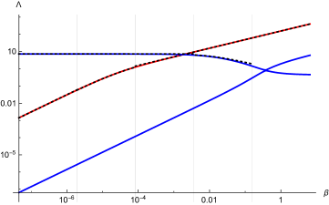
Figure 1: Summary of small wavenumber results. The numerical results for the mixed modes $\Lambda_{1}$ and $\Lambda_{2}$ are plotted in blue, while that for $\Lambda_{3}$ (the $\delta A_{\parallel}$ mode) is given in red. Ranges of $\beta$ (orders of $\epsilon$ ranging from $0$ to $4$), are separated visually by vertical gray lines at intermediate values ($\epsilon^{1/2}$, $\epsilon^{3/2}$, etc). The asymptotic results are plotted in dashed-black. Note that the growth rates are normalized to $|\omega_{i*}|$.

4.2 Intermediate wavenumber limit: $b_{i}\sim\epsilon^{-1}$, $b_{e}\sim\epsilon$

First, we note that for all $\beta$ ($\beta\sim\epsilon^{2}$, $\beta\sim\epsilon^{1}$, and $\beta\sim 1$ and larger), the expression given by Equation 37 for $\Lambda_{3}$ still applies in this limit: the ion contribution is still subdominant, and $b_{e}\ll 1$ also applies here.

For the electrostatic limit ($\beta\sim\epsilon$), we obtain

$$\Lambda_{1}^{2}=\frac{3\tau^{2}\eta_{e}^{2}\omega_{*e}^{2}}{8(\tau+1)}\\ +\frac{\tau\left(\omega_{*e}^{2}\left(6(\tau+1)\eta_{e}^{2}+4\right)+4\left(\eta_{i}-2\right)\omega_{*e}\omega_{*i}+\left(5\eta_{i}^{2}-4\eta_{i}+4\right)\omega_{*i}^{2}\right)}{16\sqrt{2\pi}(\tau+1)\sqrt{b_{i}}},$$ (39)

which can be compared with our adiabatic-electron electrostatic bound, given by Equation (6.4) of helander-plunk-jpp-part-1. Note that we need to retain the second term, formally smaller than the first by a factor $\epsilon^{1/2}$, for this comparison. The results can be made comparable by setting $\omega_{*e}=0$ and additionally taking $\omega_{*i}\rightarrow 0$ while holding $\eta_{i}\omega_{*i}\sim 1$; see the discussion following Equation 35.

For $\beta\sim 1$ we obtain (at dominant order) the result

$$\Lambda_{1,2}^{2}=\frac{\eta_{e}^{2}\omega_{*e}^{2}\left(P\pm\sqrt{P^{2}-R}\right)}{16(\tau+1)\left((\tau+2)\beta_{e}+2\right)},$$ (40)

with

$$P=\left(9\tau^{2}+23\tau+14\right)\beta_{e}^{2}-(9\tau+10)\tau\beta_{e}+6\tau^{2},$$

$$R=18\tau^{2}(\tau+1)\beta_{e}^{2}\left((\tau+2)\beta_{e}+2\right).$$

Note that the dominant (first) term of Equation 39 can be recovered as $\beta_{e}\rightarrow 0$, and that there is also an initial stabilization, as compared with the electrostatic limit associated with finite $\beta_{e}$, as can be seen in Figure 2.

We compute the critical $\beta$ as before by equating the asymptotic forms of $\Lambda_{1}$ and $\Lambda_{3}$ for the regime where they intersect, $\beta\sim\epsilon^{1}$ (retaining the first term of Eqn. 39 and the full form of Eqn. 37):

$$\beta_{e,\mathrm{crit}}=\frac{\tau b_{e}\left(\sqrt{9\tau^{2}+60(\tau+1)}+3\tau\right)}{5(\tau+1)},$$ (41)

where we have selected the positive root to that equation. Figure 2 summarizes the behavior of the roots across the beta regimes, and confirms the asymptotic results.

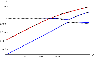
Figure 2: Summary of medium wavenumber results. The numerical results for the mixed modes $\Lambda_{1}$ and $\Lambda_{2}$ are plotted in blue, while that for $\Lambda_{3}$ (the $\delta A_{\parallel}$ mode) is given in red. Ranges of $\beta$ (orders of $\epsilon$ ranging from $0$ to $2$), are separated visually by vertical gray lines at intermediate values ($\epsilon^{1/2}$, $\epsilon^{3/2}$, etc). The asymptotic results are plotted in dashed-black. Note that the growth rates are normalized to $|\omega_{i*}|$.

4.3 Large wavenumber limit: $b_{e}\sim\epsilon^{-1}$, $b_{i}\sim\epsilon^{-3}$

For large $b_{e}$ we obtain finally an asymptotic result for $\Lambda_{3}$ distinct from the previous. For $\beta\sim\epsilon^{-1}$ or smaller we obtain,

$$\Lambda_{3}^{2}=\frac{\beta_{e}^{2}\eta_{e}^{2}\omega_{*e}^{2}}{16\pi b_{e}^{3}},$$ (42)

while for $\beta\sim\epsilon^{-2}$ we have

$$\Lambda_{3}^{2}=\frac{\beta_{e}\eta_{e}^{2}\omega_{*e}^{2}}{4\sqrt{2\pi}b_{e}^{3/2}}.$$ (43)

An electrostatic root is obtained for $\beta\sim 1$, and also survives for $\beta\sim\epsilon^{-1}$ :

$$\Lambda_{1}^{2}=\frac{\tau^{2}\eta_{e}^{2}\omega_{*e}^{2}}{8\pi(\tau+1)^{2}b_{e}}.$$ (44)

Note we do not retain higher order contributions for comparison with the adiabatic electron result, which does not discriminate between regimes of $b_{e}$, since that comparison was already made for the intermediate limit $b_{i}\sim\epsilon^{-1}$.

For $\beta\sim\epsilon^{-1}$, we find an additional electromagnetic root appears, which, curiously, matches the other electromagnetic root $\Lambda_{3}$ in this limit

$$\Lambda_{2}^{2}=\frac{\beta_{e}^{2}\eta_{e}^{2}\omega_{*e}^{2}}{16\pi b_{e}^{3}}.$$ (45)

For $\beta\sim\epsilon^{-2}$, the roots continue to match:

$$\Lambda_{2}^{2}=\frac{\beta_{e}\eta_{e}^{2}\omega_{*e}^{2}}{4\sqrt{2\pi}b_{e}^{3/2}}.$$ (46)

The critical value of $\beta$ above which the magnetic roots exceed the electrostatic one is derived as before from the results for $\beta\sim\epsilon^{-1}$:

$$\beta_{e,\mathrm{crit}}=\frac{\sqrt{2}\tau b_{e}}{\tau+1}.$$ (47)

The results of this limit are summarized in Figure 3.

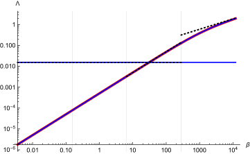
Figure 3: Summary of large wavenumber results. The numerical results for the mixed modes $\Lambda_{1}$ and $\Lambda_{2}$ are plotted in blue, while that for $\Lambda_{3}$ (the $\delta A_{\parallel}$ mode) is given in red. Ranges of $\beta$ (orders of $\epsilon$ ranging from $1$ to $-1$), are separated visually by vertical gray lines at intermediate values ($\epsilon^{1/2}$, $\epsilon^{3/2}$, etc). The asymptotic results are plotted in dashed-black. Note that the growth rates are normalized to $|\omega_{i*}|$. Note that, curiously, the red curve coincides with one branch of the blue curve, in each range of $\beta$.

5 Discussion

Although the essential ideas involved in calculating “optimal modes” are simple, the algebra involved is sufficiently complex that a general closed form solution is too lengthy to express in a useful way. Thus, we have provided a number of compact asymptotic results to demonstrate the essential behavior.

These results compare as expected with the bounds presented in helander-plunk-prl-2021 and helander-plunk-jpp-part-1, i.e. they are always less than or equal to the previous bounds, and similar qualitatively, though in some special cases much smaller. The adiabatic electron result of helander-plunk-jpp-part-1 is a curious case to compare. One might expect that the two-species electrostatic, long-wavelength limit obtained here might give a similar result, but this is not the case because the adiabatic electron response requires that the electron gyrokinetic equation be ordered and solved at the outset. Thus the two-species result is not simply a generalization of the one-species adiabatic case. On the one hand, the two species calculation is able to treat closed-field-line geometries (dipole, Z-pinch), and obtain bounds on the MHD-interchange-like instability there, whose growth tends to a constant as $k_{\perp}\rightarrow 0$; see for instance ricci-z-pinch. On the other hand, the adiabatic-electron result provides a lower bound, and compares well with expectations of the ITG mode, for which $\gamma\rightarrow 0$ as $k_{\perp}\rightarrow 0$ (kadomtsev-pogutse; biglari). This demonstrates that it is possible to improve, and reduce the complexity of the optimal mode analysis by first applying limits to the fully gyrokinetic system, as should be useful, e.g., for the case of trapped electron modes where a bounce-averaged electron response can be used.

We have assumed finite $\delta B_{\parallel}$ in our analysis, which is chiefly to blame for the added complexity of the algebra, making the results quite general for (local flux-tube) gyrokinetics. We note that its effect seems mostly subdominant to that of $\delta A_{\parallel}$ in the sense that at sufficiently low $\beta$ the electrostatic result is dominant, while at large $\beta$, a decoupled mode associated with fluctuations in $\delta A_{\parallel}$ is dominant, so that the overall maximum growth ($\max_{n}\Lambda_{n}$) is never strongly affected by the inclusion of $\delta B_{\parallel}$. Thus the weakly electromagnetic result, in which we assume $\delta B_{\parallel}\approx 0$, may be sufficient to treat many cases of interest, at least if the main goal is establishing overall bounds.

In part I and II in this series, we focus on the Helmholtz free energy, but we note that this is not the only possible choice. As we have seen, the resulting picture of stability in this case only depends on the strength of certain non-conservative terms in the gyrokinetic equation, and all that survives of the magnetic geometry is contained in the dependence of $k_{\perp}$ that enters various Bessel functions. What is lost is the mechanisms of resonance, i.e. the parallel advection and magnetic drift terms, with the latter being known to explain differences in the stability properties of different kinds of magnetic confinement devices (stellarators, tokamaks, etc.). In part III of this series, we will show how the lost effects of magnetic geometry can be recovered by use of a more generalized notion of free energy.

This work has been carried out within the framework of the EUROfusion Consortium, funded by the European Union via the Euratom Research and Training Programme (Grant Agreement No 101052200 — EUROfusion). Views and opinions expressed are however those of the author(s) only and do not necessarily reflect those of the European Union or the European Commission. Neither the European Union nor the European Commission can be held responsible for them. This work was partly supported by a grant from the Simons Foundation (560651, PH).

Appendix A ${\cal H}$ and ${\cal D}$

Taking Equations 5 and 6 and using the field equations, we obtain

$$D=\sum_{a,b}\frac{i\omega_{\ast a}}{2n_{a}n_{b}}\bigg{\langle}\int d^{3}v\int d^{3}v^{\prime}g_{a}^{*}(v)g_{b}(v^{\prime})\\ \bigg{[}\left(1-\frac{3\eta_{a}}{2}\right)\left(t_{a}t_{b}\psi_{1a}\psi_{1b}^{\prime}-\varepsilon_{a}\varepsilon_{b}\psi_{3a}\psi_{3b}^{\prime}-\varepsilon_{a}\varepsilon_{b}\psi_{5a}\psi_{5b}^{\prime}\right)\\ +\eta_{a}\left(t_{a}t_{b}\psi_{2a}\psi_{1b}^{\prime}-\varepsilon_{a}\varepsilon_{b}\psi_{4a}\psi_{3b}-\varepsilon_{a}\varepsilon_{b}\psi_{6a}\psi_{5b}\right)\bigg{]}\bigg{\rangle}+\mathrm{c.c.},$$ (48)

and

$$H=\sum_{a}\left\langle\int d^{3}v\frac{T_{a}|g_{a}|^{2}}{F_{a0}}\right\rangle-\sum_{a}\frac{1}{n_{a}T_{a}}\left\langle\left|\sum_{b}\frac{1}{n_{b}}\int d^{3}v\;t_{a}t_{b}\psi_{1b}g_{b}\right|^{2}\right\rangle\\ +\sum_{a,b}\frac{\varepsilon_{a}\varepsilon_{b}}{n_{a}n_{b}}\left\langle\int d^{3}v\int d^{3}v^{\prime}g_{a}^{*}(v)g_{b}(v^{\prime})\left[\psi_{3a}\psi_{3b}^{\prime}+\psi_{5a}\psi_{5b}^{\prime}\right]\right\rangle+\mathrm{c.c.}$$ (49)

We define the variation of an arbitrary functional $F$ with respect to the distribution function $g_{a}$ as

$$\frac{\delta F}{\delta g_{a}}=\lim_{\epsilon\rightarrow 0}\frac{d}{d\epsilon}F[g_{a}+\epsilon h],$$ (50)

where $h$ is an arbitrary function of phase space variables. Eqns. 48 and 49 yield

$$\frac{\delta D}{\delta g_{a}}=\left\langle\int d^{3}v\frac{T_{a}}{F_{a0}}h^{*}\left\{\sum_{b}{\cal D}_{ab}g_{b}\right\}\right\rangle+\mathrm{c.c.},$$ (51)

and

$$\frac{\delta H}{\delta g_{a}}=\left\langle\int d^{3}v\frac{T_{a}}{F_{a0}}h^{*}\left\{\sum_{b}{\cal H}_{ab}g_{b}\right\}\right\rangle+\mathrm{c.c.},$$ (52)

where the operators ${\cal D}$ and ${\cal H}$ are as defined in Equations 16 and 3. Note that we have exchanged species labels, and dummy velocity variables of integration to obtain this form. Because $h$ is arbitrary, these forms substituted into Equation 14 yield Equation 15.

Appendix B Bessel-type integrals

To calculate the various integrals involving Bessel functions, we begin with a general form of Weber’s integral:

$${\cal I}_{\nu}(p,a_{1},a_{2}) =\int_{0}^{\infty}\exp(-pt^{2})J_{\nu}(a_{1}t)J_{\nu}(a_{2}t)tdt$$

$$=\frac{1}{2p}\exp\left(\frac{-a_{1}^{2}-a_{2}^{2}}{4p}\right)I_{\nu}\left(\frac{a_{1}a_{2}}{2p}\right)$$ (53)

where $I_{\nu}$ is the modified Bessel function of order $\nu$. The integrals we need to evaluate can be conveniently found in terms of ${\cal I}_{\nu}$. We define

G_⟂m(b) &= 2 ∫_0^∞ x_⟂^m+1 exp(-x_⟂^2) J_0^2(2 b x_⟂^2) dx_⟂,
G_⟂m^(1)(b) = 2 ∫_0^∞ x_⟂^m+2 exp(-x_⟂^2) J_0(2 b x_⟂^2)J_1(2 b x_⟂^2) dx_⟂,
G_⟂m^(2)(b) = 2 ∫_0^∞ x_⟂^m+3 exp(-x_⟂^2) J_1^2(2 b x_⟂^2) dx_⟂, where $m$ is assumed to be even. Now we note that these integrals can be evaluated in terms of Weber’s integral:

G_⟂m(b) &= 2[ (-ddp)^m/2 I_0(p,2b,2b)]_p=1,
G_⟂m^(1)(b) = 2[ (-ddp)^m/2 (-ddλ) I_0(p,λ,2b)]_p=1, λ=