A deep learning energy method for hyperelasticity and viscoelasticity

Abstract

The potential energy formulation and deep learning are merged to solve partial differential equations governing the deformation in hyperelastic and viscoelastic materials. The presented deep energy method (DEM) is self-contained and meshfree. It can accurately capture the three-dimensional (3D) mechanical response without requiring any time-consuming training data generation by classical numerical methods such as the finite element method. Once the model is appropriately trained, the response can be attained almost instantly at any point in the physical domain, given its spatial coordinates. Therefore, the deep energy method is potentially a promising standalone method for solving partial differential equations describing the mechanical deformation of materials or structural systems and other physical phenomena.

Keywords Computational mechanics  $\cdot$ Finite deformation  $\cdot$ Meshfree method  $\cdot$ Neural networks  $\cdot$ Partial differential equations  $\cdot$ Physics-informed learning

1 Introduction

Machine learning (ML) has recently been proven effective in many fields such as image and speech recognition, medical diagnoses, autopilot in automotive scenarios, financial services, and many other engineering and medical applications [1, 2, 3]. Computational solid mechanics is no exception. Many researchers have developed data-driven models to capture physical responses [4, 5, 6, 7, 8, 9]. Additionally, data-driven models have been developed to obtain near-optimal topologies for metamaterials and structures, where 2D and 3D domains, linear and nonlinear constraints, and material and geometric nonlinearities have been considered [10, 11, 12, 13, 14]. However, usually one needs a large number of data points to accurately capture intricate relationships between the input and output, making the data generation the bottleneck step in most cases. Furthermore, deep neural networks (DNNs) have been utilized to discover governing equations and material laws using existing computational and/or experimental data [15, 16, 17].

According to the universal approximation theorem, the multilayer feedforward neural networks with an arbitrary nonconstant and bounded activation function and as few as a single hidden layer can serve, with arbitrary accuracy, as universal approximators [18, 19]. Given that the activation function is bounded, nonconstant, and continuous, then continuous mappings are uniformly learned over compact sets of inputs. Nevertheless, the theorem neither provides conclusions about the training process, nor the number of neurons required in a hidden layer to obtain a specific accuracy, nor whether the estimation of the network’s parameters is even feasible. Several successful trials have been reported for using DNNs to solve partial differential equations (PDEs), which are imperative for describing the physical laws governing all types of phenomena around us. Although solving differential equations using neural networks is not a new topic [20, 21], the recent successes are because of: 1) Recent advances in machine learning packages such as PyTorch [22] and TensorFlow [23] along with advances in CPUs and GPUs, 2) the use of automatic differentiation to accurately find the gradients of functions, and 3) the experience in choosing the networks’ architectures that can capture governing equations while satisfying initial and boundary conditions.

Recently, a number of researchers have proposed and developed frameworks to solve PDEs using DNNs, with a relatively small number of data points or even without the need for any data, by incorporating physical laws into the loss function being minimized [24, 25, 26, 27, 28, 29, 30, 31]. The approach used in these papers sometimes is referred to as the deep collocation method (DCM), as collocation points are sampled from the space of interest. Then, the DNNs attempt to find the weights and biases that best satisfy governing equations as well as initial and boundary conditions at the sampled collocation points. This approach is based on the strong form; hence, one usually needs to find second-order derivatives computationally, and the zero and nonzero natural boundary conditions should be explicitly accounted for in the loss function definition.

Weinan et al. [32] proposed a different approach to solve Poisson’s equation and eigenvalue problems. In this approach, deep learning and the Ritz method are merged to solve variational problems. Similar to the work of Weinan et al. [32], Nguyen-Thanh et al. [33] and Samaniego et al. [34] proposed a deep energy method (DEM) that utilizes potential energy to solve PDEs appearing in the field of computational solid mechanics. Nonetheless, not all governing equations can be rendered as an energy minimization problem. In the works of Weinan et al. [32], Nguyen-Thanh et al. [33], and Samaniego et al. [34], the potential energy is used to define loss functions, where only the first-order derivative is required for a second-order PDE. The advantage of this technique is that the solution procedure only requires first-order automated differentiation rather than second-order as needed for the physics-informed approach based on the strong form. This has the potential to result in faster convergence and greater accuracy. On the other hand, the approach necessitates a successful integration over the domain spanned by the collocation points.

This study extends the DEM method to solve 3-dimensional partial differential equations for materials obeying a couple of different constitutive models using deep neural networks (DNNs). In this meshfree approach, the DNN predicts the displacement field that satisfies the partial differential equations and the boundary conditions without using any labeled data. Since the training of any ML model is an optimization problem in which the loss function is minimized, we define the loss function using the potential energy. The loss function is minimized using the Adam [35] and quasi-Newton L-BFGS [36] optimizers. The DEM is used to find the mechanical response of a hyperelastic model for rubber elastic materials [37]. Additionally, the DEM is used to solve a viscoelastic model, inspired by the standard linear solid (SLS) model, by defining two potentials and casting the problem into a machine learning one. To the best of our knowledge, this is the first time that both the hyperelastic model proposed by Lopez-Pamies [37] and the SLS viscoelastic model are solved by merging the potential energy and deep learning. This meshfree approach is straightforward to implement; it does not require solving a linear system of equations and assembling the tangent modulus, which are significant steps in most computational methods, such as finite difference and finite element methods, and can be computationally expensive.

The outline of the paper is as follows: Section 2 presents the details of the approach, where a general problem setup is discussed. In Sections 3 and 4, the DEM approach is used to solve three-dimensional (3D) examples involving hyperelastic and linear viscoelastic constitutive models, respectively. We conclude the paper in Section 5 by highlighting the significant results and stating possible future work directions.

2 Method

The finite element method (FEM) is commonly used to solve problems with material and/or geometric nonlinearities. When an implicit finite element method is used along with an iterative scheme (e.g., Newton-Raphson), the residual vector and tangent matrix are assembled and then used to solve the corresponding linear system of equations, using a direct or iterative solver, to find the vector of unknowns in each iteration. On the other hand, explicit nonlinear finite element methods do not simultaneously solve a linear system; nevertheless, they are often bounded by conditional stability, requiring small time increments. Furthermore, when explicit FEM is used for quasi-static simulations, one needs to ensure that the inertial effects are insignificant [38]. This paper employs deep learning to determine the displacement field, where the displacement field obtained from the DNN is used to compute stresses, strains, and other variables required to satisfy the minimization of potential energy. Using a meshfree approach, the loss function is minimized within a deep learning framework such as PyTorch [22] and TensorFlow [23]. Subsequently, we cover a brief introduction to deep learning and then discuss the proposed framework.

2.1 Deep feedforward neural networks

Deep learning is a subset of machine learning inspired by the configuration and functionality of a brain. Deep learning models are neural networks, layers of interlinked individual unit cells, called neurons, connected to other neurons’ layers. Figure 1 shows the deep feedforward neural network, consisting of linked layers of neurons that calculate an output layer (predictions) based on input data.

Figure 1: Fully connected (dense) artificial neural network.

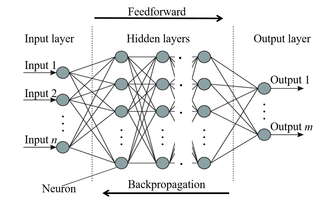
Based on the input layer, the layers of neurons propagate information forward to the successive layers, creating a learning network with some feedback mechanism. A neural network’s depth is measured by the number of hidden layers, i.e., the layers between input and output layers. Neurons of consecutive layers are connected through accompanying weights $\boldsymbol{W}$ and biases $\boldsymbol{b}$. For a layer $l$, the output $\boldsymbol{\hat{Y}}^{l}$ is calculated as:

$$\boldsymbol{Z}^{l} =\boldsymbol{W}^{l}\boldsymbol{\hat{Y}}^{l-1}+\boldsymbol{b}^{l}$$ (1)

$$\boldsymbol{\hat{Y}}^{l} =f^{l}\left(\boldsymbol{Z}^{l}\right)$$

where the weights $\boldsymbol{W}$ and biases $\boldsymbol{b}$ are updated after every training pass. The activation function $f^{l}$ is an $\mathbb{R}\rightarrow\mathbb{R}$ mapping that transforms vector $\boldsymbol{Z}^{l}$, calculated using weights and biases, into output for every neuron in the layer $l$. In neural networks, the activation functions are nonlinear functions such as sigmoid, rectified linear unit (ReLu), and hyperbolic tangent. They empower the neural network to learn nearly any multifaceted functional correlation between inputs and outputs. After each feedforward pass, the loss function $\mathcal{L}$, such as the mean square error (MSE), calculates a loss value that indicates how well the network’s predictions compare with targets.

A loss function $\mathcal{L}$ is defined, and then it is used to obtain the weights $\boldsymbol{W}$ and biases $\boldsymbol{b}$ yielding a minimized loss value. The process of determining the optimized weights and biases in the context of machine learning is called training. Backpropagation is utilized throughout the training process, wherein the loss function is minimized iteratively. One of the most prevalent and most straightforward optimizers used is gradient descent [39]:

$$W_{ij}^{c+1} =W_{ij}^{c}-\gamma\frac{\partial\,\mathcal{L}}{\partial W_{ij}^{c}}$$ (2)

$$b_{i}^{c+1} =b_{i}^{c}-\gamma\frac{\partial\,\mathcal{L}}{\partial b_{i}^{c}}$$

where $\gamma$ represents the learning rate. Equation 2 shows the formula used to update the weights $\boldsymbol{W}$ and biases $\boldsymbol{b}$ at a given iteration $c$ within the gradient descent training process.

2.2 Deep energy method

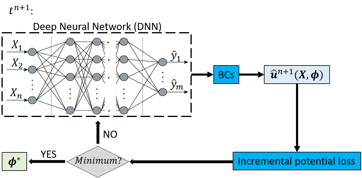
In this section, we discuss the deep energy method (DEM) in a general setting. The DEM uses an incremental potential that defines a loss function, which is minimized with the assistance of deep learning, as depicted in Figure 2. The potentials corresponding to the material models are given in the following sections.

Figure 2: Flow chart of the deep energy method (DEM) at time increment $t^{n+1}$.

We consider a generalized partial differential equation (PDE), with solution $\boldsymbol{u}\left(t,\boldsymbol{X}\right)$, expressed as:

$$\left(\partial_{t}+\mathcal{N}\right)\boldsymbol{u}\left(t,\boldsymbol{X}\right) =\boldsymbol{0}{,}\quad\left(t,\boldsymbol{X}\right)\in\left[0,T\right]\times\Omega,$$ (3)

$$\boldsymbol{u}\left(0,\boldsymbol{X}\right) =\boldsymbol{u}_{o}\quad\boldsymbol{X}\in\Omega,$$

$$\boldsymbol{u}\left(t,\boldsymbol{X}\right) =\overline{\boldsymbol{u}},\quad\!\left(t,\boldsymbol{X}\right)\in\left[0,T\right]\times\Gamma_{u},$$

$$\boldsymbol{t}\left(t,\boldsymbol{X}\right) =\overline{\boldsymbol{t}},\quad\left(t,\boldsymbol{X}\right)\in\left[0,T\right]\times\Gamma_{t},$$

where $T$ is the total time, $\partial_{t}$ is the partial derivative with respect to time $t$, $\mathcal{N}$ is a spatial differential operator, $\overline{\boldsymbol{u}}$ is a defined essential boundary condition, $\boldsymbol{u}_{o}$ is the initial condition, and $\overline{\boldsymbol{t}}$ is a defined natural boundary condition. $\Omega$ is the material domain, while $\Gamma_{t}$ and $\Gamma_{u}$ are the surfaces with natural and essential boundary conditions, respectively. Here, we attempt to solve partial differential equations by training a neural network with parameters $\boldsymbol{\phi}=\{\boldsymbol{W},\boldsymbol{b}\}$. Specifically, the model is trained such that the approximate solution $\boldsymbol{\hat{u}}\left(t,\boldsymbol{X};\boldsymbol{\phi}\right)$ obtained from the neural network minimizes the incremental potential. The examples discussed in this paper assume a quasi-static condition, i.e., the term $\partial_{t}\boldsymbol{u}=\boldsymbol{0}$ and there is no need for defining initial conditions. However, the solution $\boldsymbol{u}^{n+1}\left(\boldsymbol{X}\right)$ is obtained incrementally.

Figure 2 depicts the deep energy method used here. We cast the minimization of the loss function $\mathcal{L}$ into the optimization problem in the context of deep learning, which is commonly called training. In other words, the DNN minimizes the loss function to obtain the optimized network parameters $\boldsymbol{\phi}^{*}=\{\boldsymbol{W}^{*},\boldsymbol{b}^{*}\}$, where the loss function is defined by the incremental potential for a specific problem, and the neural network is used as global shape function for the displacement over the physical domain of interest. Specifically, the DNN maps the coordinates $\boldsymbol{X}$ of the sampled points to an output $\boldsymbol{\hat{y}}\left(\boldsymbol{X},\boldsymbol{\phi}\right)$ using the feedforward propagation. Then, there are two approaches to satisfy the essential boundary conditions. The first approach is to subject $\boldsymbol{\hat{y}}\left(\boldsymbol{X},\boldsymbol{\phi}\right)$ to:

$$\boldsymbol{\hat{u}}\left(\boldsymbol{X},\boldsymbol{\phi}\right) =\boldsymbol{A}\left(\boldsymbol{X}\right)+\boldsymbol{B}\left(\boldsymbol{X}\right)\circ\boldsymbol{\hat{y}}\left(\boldsymbol{X},\boldsymbol{\phi}\right)$$ (4)

where $\boldsymbol{A}\left(\boldsymbol{X}\right)$ and $\boldsymbol{B}\left(\boldsymbol{X}\right)$ are chosen such that the displacement field $\boldsymbol{\hat{u}}\left(\boldsymbol{X},\boldsymbol{\phi}\right)$ satisfies the essential boundary conditions active on the physical domain. More details can be found in the work of Nguyen-Thanh et al. [33] and Rao et al. [40]. The second approach to satisfy the essential boundary conditions is to set:

$$\boldsymbol{\hat{u}}\left(\boldsymbol{X},\boldsymbol{\phi}\right) =\boldsymbol{\hat{y}}\left(\boldsymbol{X},\boldsymbol{\phi}\right)$$ (5)

where one has to account for the boundary conditions throughout the training process of the DNN by adding an extra term to the loss function, as in the work of Abueidda et al. [25]. In this paper the former approach is used since the latter is a soft enforcement of the boundary conditions and does not guarantee that the boundary conditions are imposed because of the pathology issue of the gradient. The predicted displacement field $\boldsymbol{\hat{u}}$ is then used to calculate the dependent variables and loss function. The computation of the dependent variables and loss function typically requires determining the first derivative of $\boldsymbol{\hat{u}}$, which is found using the automatic differentiation offered by deep learning frameworks. The optimization (minimization) problem is written as:

$$\boldsymbol{\phi}^{*} =\underset{\boldsymbol{\phi}}{\mathrm{arg\,min}}\;\mathcal{L}\left(\boldsymbol{\phi}\right){.}$$ (6)

2.3 DNN model

We use an $8$-layer neural network (depth$=6$), where the numbers of neurons in the successive layers are $3-40-40-40-40-40-40-3$. We use three neurons in the input layer to handle 3D spatial coordinates $\boldsymbol{X}$, while we use three neurons in the output layer representing the components of the displacement vector $\boldsymbol{\hat{u}}\left(\boldsymbol{X}\right)$. The number of neurons utilized in each of the six hidden layers is $nHL=40$. An activation function was used after each layer, as demonstrated in Equation 1. The architecture of the network is obtained by trying several architectures and fine-tuning of hyperparameters.

Abandoning nonlinear activation functions reduces the network to a linear one, making it challenging to capture nonlinear relationships between input and output. For example, some popular activation functions, in many machine learning practices, are ReLU and leaky ReLU. This paper uses a ReLU activation function in the input and hidden layers, while we use a linear activation function in the output layer.

In this paper, we use PyTorch to solve the deep learning problem (minimize the loss function). The two optimizers are employed in a serial fashion; the Adam optimizer is initially used, and then the limited-memory BFGS (L-BFGS) optimizer with the Strong Wolfe line search method [36, 41] is utilized. We found that using both optimizers regularly stabilizes the optimization procedure; a similar conclusion was sketched in other papers in the literature [25, 26]. More details are discussed in the following sections.

3 Hyperelasticity

We consider a body made of a homogeneous and isotropic hyperelastic material under finite deformation. The mapping $\boldsymbol{\zeta}$ of material points from the initial configuration to the current configuration is determined by:

$$\boldsymbol{x} =\boldsymbol{\zeta}\left(\boldsymbol{X},t\right)=\boldsymbol{X}+\boldsymbol{\hat{u}}.$$ (7)

Assuming that body and inertial forces are absent, the strong form is expressed as:

$$\begin{split}\boldsymbol{\nabla}_{\boldsymbol{X}}\cdot\boldsymbol{P}&=\boldsymbol{0}{,}\quad\boldsymbol{X}\in\Omega,\\ \boldsymbol{\hat{u}}&=\overline{\boldsymbol{u}},\quad\!\boldsymbol{X}\in\Gamma_{u},\\ \boldsymbol{P}\cdot\boldsymbol{N}&=\overline{\boldsymbol{t}},\quad\boldsymbol{X}\in\Gamma_{t},\\ \end{split}$$ (8)

where $\boldsymbol{\nabla}_{\boldsymbol{X}}\cdot$ is the divergence operator, $\boldsymbol{P}$ is the first Piola-Kirchhoff stress, and $\boldsymbol{N}$ represents the outward normal unit vector in the initial configuration. $\overline{\boldsymbol{u}}$ accounts for a defined essential boundary condition, and $\overline{\boldsymbol{t}}$ presents a defined natural boundary condition. $\Omega$ denotes the material domain, while $\Gamma_{u}$ and $\Gamma_{t}$ are the surfaces with essential and natural boundary conditions, respectively. The constitutive law for such a material is expressed as:

$$\boldsymbol{P} =\frac{\partial\psi\left(\boldsymbol{F}\right)}{\partial\boldsymbol{F}}$$ (9)

$$\boldsymbol{F} =\boldsymbol{\nabla}_{\boldsymbol{X}}\boldsymbol{\zeta}\left(\boldsymbol{X}\right)$$

where $\psi$ is the strain energy density of a specific material, and $\boldsymbol{F}$ denotes the deformation gradient. The material model of interest was proposed by Lopez-Pamies [37]. The strain energy model is given by:

$$\psi =\sum_{r=1}^{M}\frac{3^{1-\alpha_{r}}}{2\alpha_{r}}\mu_{r}\left(I_{1}^{\alpha_{r}}-3^{\alpha_{r}}\right)-\sum_{r=1}^{M}\mu_{r}\text{ln}J+\frac{\lambda}{2}\left(J-1\right)^{2}$$ (10)

where $I_{1}$ is the the first principal invariant of the right Cauchy–Green deformation tensor $\boldsymbol{C}$, i.e., $I_{1}=\text{trace}\left(\boldsymbol{C}\right)$. The right Cauchy–Green deformation tensor $\boldsymbol{C}$ is expressed as $\boldsymbol{C}=\boldsymbol{F}^{T}\boldsymbol{F}$, where $\left(\right)^{T}$ is the transpose operator. $M$ represents the number of terms included in the summation, while $\alpha_{r}$, $\mu_{r}$ and $\lambda$ are material constants $\left(r=1,2,...,M\right)$. $J$ is the determinant of the deformation gradient. We aim here at developing a DNN model that (1) is straightforward and amenable to numerical and analytical solutions for boundary-value and homogenization problems, (2) contains material constants providing a physical interpretation, and (3) characterizes and accurately predicts the mechanical behavior of rubber-like elastic solids over the entire range of deformations [37]. The constitutive relation implied by the potential shown in Equation (10) is expressed as:

$$\boldsymbol{P} =\frac{\partial\psi\left(\boldsymbol{F}\right)}{\partial\boldsymbol{F}}=\sum_{r=1}^{M}3^{1-\alpha_{r}}\mu_{r}I_{1}^{\alpha_{r}-1}\boldsymbol{F}-\sum_{r=1}^{M}\mu_{r}\boldsymbol{F}^{-T}+\lambda\left(J^{2}-J\right)\boldsymbol{F}^{-T}$$ (11)

In this paper, the number of terms $M$ in Equation (10) is $M=2$. Following the deep energy method, one needs no incremental tangent modulus since we do not solve a linear system of equations here, as in the case of classical finite element problems. Hence, we do not include it.

To solve a hyperelasticity problem, we transform the strong form (see Equation (8)) into the weak form. However, for a hyperelastic material, the weak form can be expressed as:

$$\Pi=\underbrace{\int_{\Omega}\psi d\Omega}_{\text{internal energy}}\underbrace{-\int_{\Omega}\boldsymbol{u}^{T}\boldsymbol{f}_{b}d\Omega-\int_{\Gamma}\boldsymbol{u}^{T}\overline{\boldsymbol{t}}d\Gamma}_{\text{external energy}}$$ (12)

For hyperelastic materials, we aim at minimizing the potential energy, shown in Equation (12), where the loss function to be minimized is defined as:

$$\mathcal{L}=\int_{\Omega}\hat{\psi}\left(\boldsymbol{X},\boldsymbol{\phi}\right)d\Omega-\int_{\Omega}\boldsymbol{\hat{u}}^{T}\left(\boldsymbol{X},\boldsymbol{\phi}\right)\;\boldsymbol{f}_{b}d\Omega-\int_{\Gamma}\boldsymbol{\hat{u}}^{T}\left(\boldsymbol{X},\boldsymbol{\phi}\right)\;\overline{\boldsymbol{t}}d\Gamma$$ (13)

where the body force $\boldsymbol{f}_{b}$ is assumed to be negligible in this work, and $\boldsymbol{\hat{u}}\left(\boldsymbol{X},\boldsymbol{\phi}\right)$ is the approximate displacement obtained from the neural network, as shown in Figure 2. A numerical integration scheme has to be used to calculate the loss function. In this work, we have used the 3D trapezoidal rule to evaluate the integrals defining the loss function shown in Equation (13). Algorithm 1 summarizes the steps involved in solving hyperelastic problems.

Input: Physical domain, BCs, and DNN

  Material parameters ($\lambda,\mu_{1},\mu_{2},\alpha_{1},\alpha_{2}$)

  Sample points $\boldsymbol{X}_{int}$ from $\Omega$

  Sample points $\boldsymbol{X}_{u}$ from $\Gamma_{u}$

  Sample points $\boldsymbol{X}_{t}$ from $\Gamma_{t}$

  Neural network architecture

  Neural network hyperparameters

  Optimizer (Adam followed by L-BFGS)

Initialization: Initial weights and biases of the DNN

Output: Optimized weights and biases of the DNN

while Not minimized do

       Obtain $\boldsymbol{\hat{u}}$ from the DNN

       Compute $\boldsymbol{\nabla}_{\boldsymbol{X}}\boldsymbol{\hat{u}}$ using automatic differentiation

       Compute $\boldsymbol{F}=\boldsymbol{I}+\boldsymbol{\nabla}_{\boldsymbol{X}}\boldsymbol{\hat{u}}$

       Compute $J=\text{det}\left(\boldsymbol{F}\right)$, $\boldsymbol{C}$, $I_{1}$, and $\boldsymbol{P}$

       Calculate loss function

       Update the weights and biases

      

end while

Algorithm 1 Hyperelasticity pseudocode.

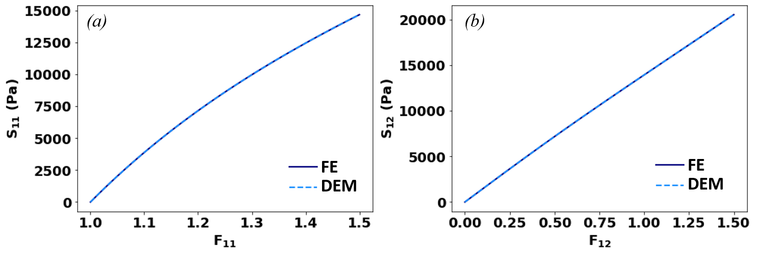
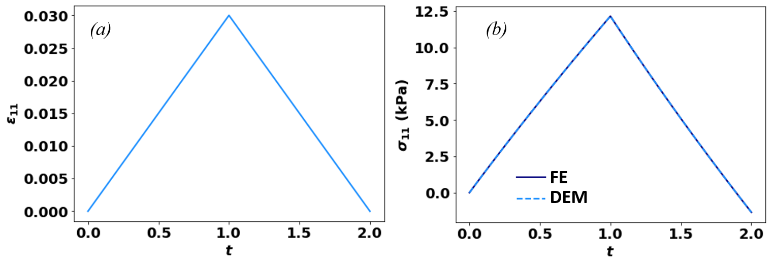
For illustrational purposes, we consider two scenarios: (1) a cube with unit length subject to a uniaxial tensile loading and (2) a cube with unit length subject to a simple shear loading. The material properties used are as follows: $\alpha_{1}=1.0$, $\alpha_{2}=-2.47$, $\mu_{1}=13.5$ kPa, $\mu_{2}=1.08$ kPa, and $\lambda=146.2$ kPa.

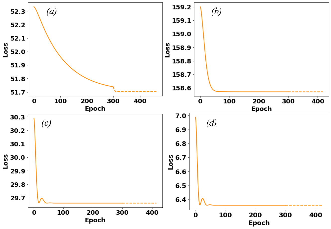
Here, we use a displacement-controlled approach. Considering a unit cube incrementally subject to a uniaxial strain of 0.5, the effect of the number of points, evenly spaced in the physical domain, on the convergence of the loss function is studied. The main reason for using evenly spaced points rather than randomly sampled points is to make the numerical integrations required to evaluate the loss function more straightforward. Figure 3 shows the convergence of the loss function. We have considered two problem sizes: $25\times 25\times 25=15625$ points and $30\times 30\times 30=27000$. Generally, we do not see a significant change in the converged values of the loss function when different numbers of points are taken from the physical domain. As discussed earlier, we have used two optimizers: the Adam optimizer followed by L-BFGS optimizer. For the Adam optimizer, we have used a fixed number, $300$ epochs, while for the L-BFGS optimizer, a tolerance of $1e-12$ was used as a stopping criterion. The solution is attained for $N$ displacement increments. Hence, the optimization problem is solved $N$ times. The optimized weights and biases found at increment $t$ are utilized to initialize weights and biases for the next increment $t+1$. This approach can be viewed as a form of transfer learning in the context and terminologies of machine learning, which is equivalent to updating displacements after each converged increment in any classical nonlinear implicit finite element analysis solution procedure. Due to the use of transfer learning, we observe that the convergence at later increments is faster and easier than those at the beginning, unlike the finite element method. Generally, we do not see a significant change in the convergence of the neural network discussed in section 2.3 when different numbers of points are taken from the physical domain.

Figure 3: Hyperelasticity example (unit cube): Loss function convergence for different problem sizes (number of points). The solid lines represent the loss history obtained using the Adam optimizer, while the dashed lines portray loss history obtained from the L-BFGS optimizer. Different uniaxial strains are imposed: (a) $0.125$, (b) $0.25$, (c) $0.375$, and (d) $0.5$.

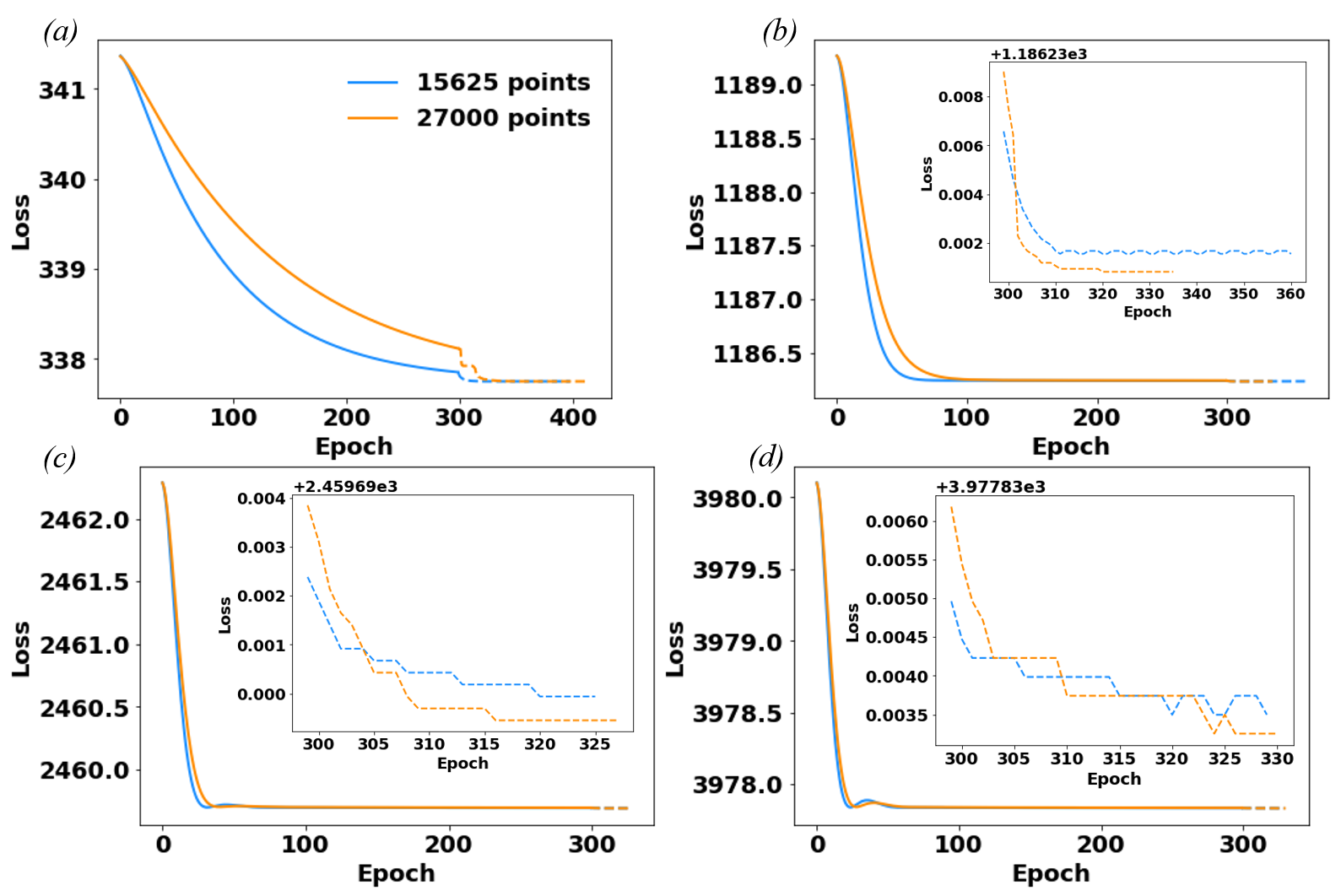
Figure 4a depicts a comparison between the solutions obtained from the traditional finite element analysis and the DEM. The DEM manages to capture the stress-deformation curve qualitatively and quantitatively. A similar analysis was done for the simple shear case, and similar conclusions were deduced. For the sake of brevity, we just include the final results, as shown in Figure 4b. Since the hyperelasticity problem is path-independent, the DEM method does not require incremental loading. However, in classical finite element analysis, the problem is still solved incrementally in many cases to avoid divergence issues which we do not see in the DEM method. Hence, if one is not interested in the intermediate evaluations, the DEM can solve the problem in one increment without having a pseudo time loop, as summarized in Algorithm 1. However, in this paper, we are interested in the entire curve (see Figure 4), which we have solved incrementally using transfer learning as discussed earlier.

Figure 4: Comparison between the DEM and FEM results: Unit cube Subject to (a) uniaxial displacement and (b) simple shear.

4 Viscoelasticity

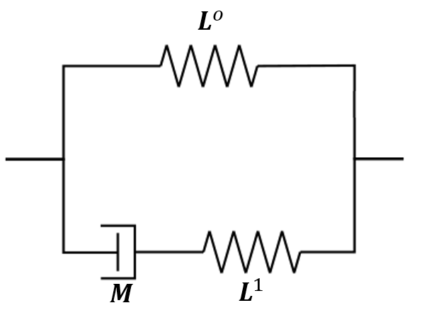
We consider a 3D homogeneous, isotropic, linear viscoelastic model consistent with the standard linear solid (SLS) model depicted in Figure 5 under small deformation. The equilibrium equation, in the absence of inertial and body forces, is written as:

$$\begin{split}\boldsymbol{\nabla}\cdot\boldsymbol{\sigma}&=\boldsymbol{0}{,}\quad\boldsymbol{x}\in\Omega,\\ \boldsymbol{\hat{u}}&=\overline{\boldsymbol{u}},\quad\!\boldsymbol{x}\in\Gamma_{u},\\ \boldsymbol{\sigma}\cdot\boldsymbol{n}&=\overline{\boldsymbol{t}},\quad\boldsymbol{x}\in\Gamma_{t},\\ \end{split}$$ (14)

where $\boldsymbol{\sigma}$ denotes the Cauchy stress tensor, $\boldsymbol{n}$ is the normal unit vector, $\boldsymbol{\nabla}\cdot$ is the divergence operator, and $\boldsymbol{\nabla}$ represents the gradient operator. Since small deformation is assumed, the strain tensor $\boldsymbol{\varepsilon}$ is expressed as:

$$\boldsymbol{\varepsilon}=\frac{1}{2}(\boldsymbol{\nabla}\boldsymbol{\hat{u}}+\boldsymbol{\nabla}\boldsymbol{\hat{u}}^{T}).$$ (15)

We adopt a two-potential constitutive framework to describe how a material stores and dissipates energy by defining two thermodynamic potentials: (1) a free energy function $\psi$ and (2) a dissipation potential $\eta$. The two potentials are defined by the equilibrium modulus of elasticity $\boldsymbol{L}^{o}$, the non-equilibrium modulus of elasticity $\boldsymbol{L}^{1}$, and the viscosity tensor $\boldsymbol{M}$. Assuming an isotropic material, the fourth-order tensors $\boldsymbol{L}^{o}$, $\boldsymbol{L}^{1}$, and $\boldsymbol{M}$ can be expressed as:

$$L^{o}_{ijkl} =2\mu_{o}\mathcal{K}_{ijkl}+3\kappa_{o}\mathcal{J}_{ijkl}$$ (16)

$$L^{1}_{ijkl} =2\mu_{1}\mathcal{K}_{ijkl}+3\kappa_{1}\mathcal{J}_{ijkl}$$

$$M_{ijkl} =2\omega_{K}\mathcal{K}_{ijkl}+3\omega_{J}\mathcal{J}_{ijkl}$$

with $\mathcal{K}_{ijkl}$ and $\mathcal{J}_{ijkl}$ defined as:

$$\mathcal{K}_{ijkl} =\frac{1}{2}\left(\delta_{ik}\delta_{jl}+\delta_{il}\delta_{jk}-\frac{2}{3}\delta_{ij}\delta_{kl}\right)$$ (17)

$$\mathcal{J}_{ijkl} =\frac{1}{3}\delta_{ij}\delta_{kl}$$

where $\delta_{ij}$ denotes the Kronecker delta, $\mu$ is the shear modulus, $\kappa$ represents the bulk modulus, $\omega_{K}$ is the distortional viscosity, and $\omega_{J}$ is the volumetric viscosity.

Figure 5: Rheological model of linear viscoelastic behavior.

The two thermodynamic potentials used to define the viscoelastic model are:

$$\psi =\frac{1}{2}\varepsilon_{ij}L^{o}_{ijkl}\varepsilon_{kl}+\frac{1}{2}\left(\varepsilon_{ij}-\varepsilon^{v}_{ij}\right)L^{1}_{ijkl}\left(\varepsilon_{kl}-\varepsilon^{v}_{kl}\right)$$ (18)

$$=\mu_{o}\varepsilon_{ij}\varepsilon_{ij}+\frac{3\kappa_{o}-2\mu_{o}}{6}\varepsilon_{ii}\varepsilon_{jj}+\mu_{1}\varepsilon^{e}_{ij}\varepsilon^{e}_{ij}+\frac{3\kappa_{1}-2\mu_{1}}{6}\varepsilon^{e}_{ii}\varepsilon^{e}_{jj}$$

$$\eta =\frac{1}{2}\dot{\varepsilon}^{v}_{ij}M_{ijkl}\dot{\varepsilon}^{v}_{kl}$$

$$=\omega_{K}\dot{\varepsilon}^{v}_{ij}\dot{\varepsilon}^{v}_{ij}+\frac{3\omega_{J}-2\omega_{K}}{6}\dot{\varepsilon}^{v}_{ii}\dot{\varepsilon}^{v}_{jj}$$

where $\boldsymbol{\varepsilon}^{v}$ is the viscous part of the total strain $\boldsymbol{\varepsilon}$, and $\boldsymbol{\varepsilon}^{e}=\boldsymbol{\varepsilon}-\boldsymbol{\varepsilon}^{v}$ is the elastic part obtained from the additive decomposition. The constitutive relation implied by the above potentials is given by:

$$\sigma_{ij} =\frac{\partial\psi}{\partial\varepsilon_{ij}}=L^{o}_{ijkl}\varepsilon_{kl}+L^{1}_{ijkl}\left(\varepsilon_{kl}-\varepsilon^{v}_{kl}\right)$$ (19)

$$=2\mu_{o}\varepsilon_{ij}+\frac{3\kappa_{o}-2\mu_{o}}{3}\varepsilon_{kk}\delta_{ij}+2\mu_{1}\left(\varepsilon_{ij}-\varepsilon^{v}_{ij}\right)+\frac{3\kappa_{1}-2\mu_{1}}{3}\left(\varepsilon_{kk}-\varepsilon^{v}_{kk}\right)\delta_{ij}$$

where the internal variable $\varepsilon^{v}_{kl}$ is implicitly defined by the evolution equation:

$$\frac{\partial\psi}{\partial\varepsilon^{v}_{ij}}+\frac{\partial\eta}{\partial\dot{\varepsilon}^{v}_{ij}} =0$$ (20)

$$-L^{1}_{ijkl}\left(\varepsilon_{kl}-\varepsilon^{v}_{kl}\right)+M_{ijkl}\dot{\varepsilon}^{v}_{kl} =0$$

or equivalently:

$$\dot{\varepsilon}^{v}_{ij} =M^{-1}_{ijmn}L^{1}_{mnkl}\left(\varepsilon_{kl}-\varepsilon^{v}_{kl}\right)$$ (21)

$$=\frac{\mu_{1}}{\omega_{K}}\left(\varepsilon_{ij}-\varepsilon^{v}_{ij}\right)+\frac{1}{3}\left(\frac{\kappa_{1}}{\omega_{J}}-\frac{\mu_{1}}{\omega_{K}}\right)\left(\varepsilon_{kk}-\varepsilon^{v}_{kk}\right)\delta_{ij}\doteq G_{ij}\left(t,\boldsymbol{\varepsilon}^{v}\right)$$

where the function $\boldsymbol{G}$, as a function of time $t$ and internal variable $\boldsymbol{\varepsilon}^{v}$, is defined for subsequent notational brevity.

The solution for the problem of interest is obtained by defining the following incremental potential:

$$\Pi =\int_{\Omega}\psi\left(\boldsymbol{\varepsilon},\boldsymbol{\varepsilon}^{v}\right)d\Omega+\Delta t\int_{\Omega}\eta\left(\dot{\boldsymbol{\varepsilon}}^{v}\right)d\Omega-\int_{\Omega}\boldsymbol{u}^{T}\boldsymbol{f}_{b}d\Omega-\int_{\Gamma}\boldsymbol{u}^{T}\overline{\boldsymbol{t}}d\Gamma$$ (22)

where $\Delta t=t^{n+1}-t^{n}$. Assuming that the body forces $\boldsymbol{f}_{b}$ are zero and introducing the backward-Euler approximation:

$$\dot{\boldsymbol{\varepsilon}}^{v} \approx\frac{\boldsymbol{\varepsilon}^{v,n+1}-\boldsymbol{\varepsilon}^{v,n}}{\Delta t}$$ (23)

into the dissipation potential, the incremental loss function is given by:

$$\mathcal{L}^{n+1} =\int_{\Omega}\psi\left(\boldsymbol{\varepsilon}^{n+1},\boldsymbol{\varepsilon}^{v,n+1}\right)d\Omega+\Delta t\int_{\Omega}\eta\left(\frac{\boldsymbol{\varepsilon}^{v,n+1}-\boldsymbol{\varepsilon}^{v,n}}{\Delta t}\right)d\Omega-\int_{\Gamma}{\boldsymbol{u}^{n+1}}^{T}\overline{\boldsymbol{t}}^{n+1}d\Gamma$$ (24)

where $\boldsymbol{\varepsilon}^{v,n+1}$ is computed using the explicit fifth-order Runge–Kutta scheme with extended region of stability [42], which is given by:

$$\boldsymbol{\varepsilon}^{v,n+1} =\boldsymbol{\varepsilon}^{v,n}+\frac{\Delta t}{90}\left(7\boldsymbol{k}_{1}+32\boldsymbol{k}_{3}+12\boldsymbol{k}_{4}+32\boldsymbol{k}_{5}+7\boldsymbol{k}_{6}\right)$$ (25)

where

$$\boldsymbol{k}_{1} =\boldsymbol{G}\left(t_{n},\boldsymbol{\varepsilon}^{v,n}\right)$$ (26)

$$\boldsymbol{k}_{2} =\boldsymbol{G}\left(t_{n}+\frac{\Delta t}{2},\boldsymbol{\varepsilon}^{v,n}+\boldsymbol{k}_{1}\frac{\Delta t}{2}\right)$$

$$\boldsymbol{k}_{3} =\boldsymbol{G}\left(t_{n}+\frac{\Delta t}{4},\boldsymbol{\varepsilon}^{v,n}+\left(3\boldsymbol{k}_{1}+\boldsymbol{k}_{2}\right)\frac{\Delta t}{16}\right)$$

$$\boldsymbol{k}_{4} =\boldsymbol{G}\left(t_{n}+\frac{\Delta t}{2},\boldsymbol{\varepsilon}^{v,n}+\boldsymbol{k}_{3}\frac{\Delta t}{2}\right)$$

$$\boldsymbol{k}_{5} =\boldsymbol{G}\left(t_{n}+\frac{3\Delta t}{2},\boldsymbol{\varepsilon}^{v,n}+3\left(-\boldsymbol{k}_{2}+2\boldsymbol{k}_{3}+3\boldsymbol{k}_{4}\right)\frac{\Delta t}{16}\right)$$

$$\boldsymbol{k}_{6} =\boldsymbol{G}\left(t_{n}+\Delta t,\boldsymbol{\varepsilon}^{v,n}+\left(\boldsymbol{k}_{1}+4\boldsymbol{k}_{2}+6\boldsymbol{k}_{3}-12\boldsymbol{k}_{4}+8\boldsymbol{k}_{5}\right)\frac{\Delta t}{7}\right).$$

The procedure used to solve the viscoelastic problem is described in Algorithm 2. For viscoelastic problems, the solution is obtained using $M$ time steps. Hence, the optimization problem is solved $M$ times, where we use transfer learning such that the converged weights and biases obtained at the increment $t^{n}$ are used to initialize the DNN at the following increment $t^{n+1}$.

Input: Physical domain, BCs, and DNN

  Material parameters ($\kappa_{o}$, $\kappa_{1}$, $\mu_{o}$, $\mu_{1}$, $\omega_{K}$, and $\omega_{J}$)

  Sample points $\boldsymbol{X}_{int}$ from $\Omega$

  Sample points $\boldsymbol{X}_{u}$ from $\Gamma_{u}$

  Sample points $\boldsymbol{X}_{t}$ from $\Gamma_{t}$

  Neural network architecture

  Neural network hyperparameters

  Optimizer (Adam followed by L-BFGS)

  Initialize $\boldsymbol{\varepsilon}^{v}$

Initialization: Initial weights and biases of the DNN

Output: Optimized weights and biases of the DNN

for $t\leftarrow 1$ to number of steps do

       Use weights and biases from previous step

       while Not minimized do

             Obtain $\boldsymbol{\hat{u}}$ from the DNN

             Compute $\boldsymbol{\nabla}\boldsymbol{\hat{u}}$ using automatic differentiation

             Compute $\boldsymbol{\varepsilon}^{v}$ using the evolution equation

             Determine $\psi$ and $\eta$

             Calculate loss function

             Update the weights and biases

            

       end while

      

end for

Algorithm 2 Linear viscoelasticity pseudocode.

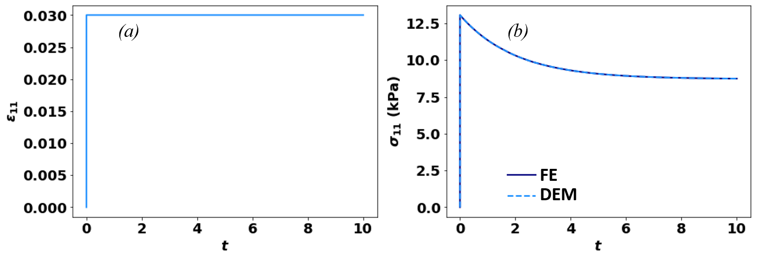
Let’s consider a unit cube under a loading and unloading uniaxial test. Specifically, it is incrementally subjected to a strain of 3% in 1 s, and then it has been unloaded to a strain of 0% in another 1 s. Figure 6 shows the convergence of the loss function at different strains. Figure 7 presents the history of the applied strain as well as the stress history. Another example we consider in this paper is the relaxation test. Figure 8 depicts the applied strain and the relaxation of stress. The finite element results and those obtained from the DEM are in agreement in both test cases.

Figure 6: Two-potential viscoelasticity example (unit cube): Loss function convergence. The solid lines represent the loss history obtained using the Adam optimizer, while the dashed lines portray loss history obtained from the L-BFGS optimizer. Firstly, the cube is subject to a uniaxial strain of: (a) $1.5\%$ (at $t=0.5$ s) and (b) $3\%$ (at $t=1.0$ s). Then, it has been incrementally unloaded to a strain of (c) $1.5\%$ (at $t=1.5$ s) and (d) $0\%$ (at $t=2.0$ s).

Figure 7: Loading and unloading: (a) History of the applied strain and (b) comparison between the results obtained from the FE analysis and DEM.

5 Discussion, conclusions, and future directions

Figure 8: Relaxation test: (a) History of the applied strain and (b) comparison between the stress obtained from the FE analysis and DEM.

In this study, the potential energy and deep learning are coupled to solve partial differential equations governing the mechanical deformation of hyperelastic and viscoelastic materials. Specifically, the first pillar of the DEM is that the potential energy that describes the mechanical deformation in a physical domain constitutes the basis for the construction of the loss function. The second pillar of the DEM is that the DNN defines the approximation space. When we solve for a hyperelastic response, the potential energy is minimized using deep learning tools. However, in the case of a viscoelastic response, an incremental potential, based on the two-potential approach, has to be defined and minimized. It is worth noting that this is one of the first implementations of 3D nonlinear solid mechanics using physics-informed neural networks. Using this approach, no data is created, which is often the bottleneck stage in constructing a data-driven model, and instead, the deep energy method (DEM) is used to get the solution. Compared to the physics-informed solution based on the strong form, the DEM solution is generally smoother. Furthermore, the DEM is meshfree; hence, we do not define connectivity between the nodes and mesh generation, which can be challenging in many cases [43] and may necessitate partitioning methods for large meshes [44]. Also, meshfree methods do not encounter the issue of element distortion or volumetric locking.

As stated in Section 2.1, the deep learning approach is based mainly on matrix-vector multiplications, which are highly well-tuned and execute on GPUs. Unfortunately, this is not the case with direct sparse solvers in the implicit finite element method, which are frequently the only robust solver technique, but to date, it fails to make full use of GPUs. For nonlinear high fidelity simulations with millions of degrees of freedom, it is realistic to predict that physics-informed neural networks using transfer learning on GPUs may outperform a traditional implicit finite element technique. Additionally, writing from scratch a physics-informed neural network to solve PDEs is much easier and quicker than writing a nonlinear finite element code. Finally, a combination of data-driven and physics-informed deep learning approaches has been used to solve incomplete and ill-posed problems in computational mechanics and other physics-based modeling disciplines, previously considered insolvable by the classical numerical methods [45].

Other geometries, such as irregular 3D geometries, will be examined in future studies. High-gradient solution regions appear when the geometries get more complicated. A new extended deep energy formulation, known as the mixed deep energy method (mDEM) [46], has been developed recently that predicts stresses in addition to displacements from the neural network and delivers more accurate findings in high-gradient solution portions of domains, such as stress concentrations. Another limitation of this work is that we picked evenly spaced points from the physical domain to make the numerical integrations required to evaluate the loss functions straightforward. However, in principle, one can adopt other random sampling techniques (such as Latin hypercube, Halton sequence, etc.) along with more sophisticated numerical integration schemes to investigate how different sampling techniques impact the model’s performance and explore which ones lead to higher accuracy. Guo et al. [26] studied the effect of sampling techniques in the context of the deep collocation method (DCM), and it would be interesting to examine this effect in the context of the DEM.

The optimization problems solved using the DCM or DEM are often non-convex. Hence, one must be attentive to getting trapped in local minima. Nonconvexity leads to several challenges that have to be investigated by the mechanics community. Additionally, in this paper, the architecture of the network and hyperparameters are chosen on a trial and error basis. However, one needs an architecture and hyperparameters that provide good accuracy and requires the architecture and hyperparameters to be optimized to get the highest performance possible. Hamdia et al. [47] suggested using the genetic algorithm to find the optimized architecture and hyperparameters. Solving PDEs with physics-informed deep learning techniques is currently a growing trend within the research community, and our paper is by no means the final word on the subject.

Data availability

The data that support the findings of this study are available from the corresponding author upon reasonable request.

References

- [1] W. Lim, D. Jang, T. Lee, Speech emotion recognition using convolutional and recurrent neural networks, in: 2016 Asia-Pacific signal and information processing association annual summit and conference (APSIPA), IEEE, 2016, pp. 1–4.
- [2] Z. Thorat, S. Mahadik, S. Mane, S. Mohite, A. Udugade, Self driving car using raspberry-Pi and machine learning, International Research Journal of Engineering and Technology 6 (2019) 969–972.
- [3] M. de Bruijne, Machine learning approaches in medical image analysis: From detection to diagnosis, Medical Image Analysis 33 (2016) 94 – 97.
- [4] M. Mozaffar, R. Bostanabad, W. Chen, K. Ehmann, J. Cao, M. Bessa, Deep learning predicts path-dependent plasticity, Proceedings of the National Academy of Sciences 116 (52) (2019) 26414–26420.
- [5] D. W. Abueidda, S. Koric, N. A. Sobh, H. Sehitoglu, Deep learning for plasticity and thermo-viscoplasticity, International Journal of Plasticity 136 (2021) 102852.
- [6] A. D. Spear, S. R. Kalidindi, B. Meredig, A. Kontsos, J.-B. Le Graverend, Data-driven materials investigations: The next frontier in understanding and predicting fatigue behavior, JOM 70 (7) (2018) 1143–1146.
- [7] D. W. Abueidda, M. Almasri, R. Ammourah, U. Ravaioli, I. M. Jasiuk, N. A. Sobh, Prediction and optimization of mechanical properties of composites using convolutional neural networks, Composite Structures 227 (2019) 111264.
- [8] S. M. Sadat, R. Y. Wang, A machine learning based approach for phononic crystal property discovery, Journal of Applied Physics 128 (2) (2020) 025106.
- [9] S. Koric, D. W. Abueidda, Deep learning sequence methods in multiphysics modeling of steel solidification, Metals 11 (3) (2021) 494.
- [10] D. W. Abueidda, S. Koric, N. A. Sobh, Topology optimization of 2D structures with nonlinearities using deep learning, Computers & Structures 237 (2020) 106283.
- [11] S. Zheng, Z. He, H. Liu, Generating three-dimensional structural topologies via a u-net convolutional neural network, Thin-Walled Structures (2020) 107263.
- [12] L. Wang, Y.-C. Chan, F. Ahmed, Z. Liu, P. Zhu, W. Chen, Deep generative modeling for mechanistic-based learning and design of metamaterial systems, Computer Methods in Applied Mechanics and Engineering 372 (2020) 113377.
- [13] H. T. Kollmann, D. W. Abueidda, S. Koric, E. Guleryuz, N. A. Sobh, Deep learning for topology optimization of 2D metamaterials, Materials & Design 196 (2020) 109098.
- [14] Q. Lin, J. Hong, Z. Liu, B. Li, J. Wang, Investigation into the topology optimization for conductive heat transfer based on deep learning approach, International Communications in Heat and Mass Transfer 97 (2018) 103–109.
- [15] J. Zhao, J. Mau, Discovery of governing equations with recursive deep neural networks, arXiv preprint arXiv:2009.11500.
- [16] H. Yang, Q. Xiang, S. Tang, X. Guo, Learning material law from displacement fields by artificial neural network, Theoretical and Applied Mechanics Letters 10 (3) (2020) 202–206.
- [17] M. Flaschel, S. Kumar, L. De Lorenzis, Unsupervised discovery of interpretable hyperelastic constitutive laws, arXiv preprint arXiv:2010.13496.
- [18] G. Cybenko, Approximation by superpositions of a sigmoidal function, Mathematics of control, signals and systems 2 (4) (1989) 303–314.
- [19] K. Hornik, Approximation capabilities of multilayer feedforward networks, Neural networks 4 (2) (1991) 251–257.
- [20] A. J. Meade Jr, A. A. Fernandez, The numerical solution of linear ordinary differential equations by feedforward neural networks, Mathematical and Computer Modelling 19 (12) (1994) 1–25.
- [21] I. E. Lagaris, A. Likas, D. I. Fotiadis, Artificial neural networks for solving ordinary and partial differential equations, IEEE transactions on neural networks 9 (5) (1998) 987–1000.
- [22] A. Paszke, S. Gross, F. Massa, A. Lerer, J. Bradbury, G. Chanan, T. Killeen, Z. Lin, N. Gimelshein, L. Antiga, A. Desmaison, A. Kopf, E. Yang, Z. DeVito, M. Raison, A. Tejani, S. Chilamkurthy, B. Steiner, L. Fang, J. Bai, S. Chintala, Pytorch: An imperative style, high-performance deep learning library, in: H. Wallach, H. Larochelle, A. Beygelzimer, F. d'Alché-Buc, E. Fox, R. Garnett (Eds.), Advances in Neural Information Processing Systems 32, Curran Associates, Inc., 2019, pp. 8024–8035.
- [23] M. Abadi, A. Agarwal, P. Barham, E. Brevdo, Z. Chen, C. Citro, G. S. Corrado, A. Davis, J. Dean, M. Devin, S. Ghemawat, I. Goodfellow, A. Harp, G. Irving, M. Isard, Y. Jia, R. Jozefowicz, L. Kaiser, M. Kudlur, J. Levenberg, D. Mané, R. Monga, S. Moore, D. Murray, C. Olah, M. Schuster, J. Shlens, B. Steiner, I. Sutskever, K. Talwar, P. Tucker, V. Vanhoucke, V. Vasudevan, F. Viégas, O. Vinyals, P. Warden, M. Wattenberg, M. Wicke, Y. Yu, X. Zheng, TensorFlow: Large-scale machine learning on heterogeneous systems, software available from tensorflow.org (2015).
- [24] M. Raissi, P. Perdikaris, G. E. Karniadakis, Physics-informed neural networks: A deep learning framework for solving forward and inverse problems involving nonlinear partial differential equations, Journal of Computational Physics 378 (2019) 686–707.
- [25] D. W. Abueidda, Q. Lu, S. Koric, Meshless physics-informed deep learning method for three-dimensional solid mechanics, International Journal for Numerical Methods in Engineering 122 (23) (2021) 7182–7201.
- [26] H. Guo, X. Zhuang, X. Meng, T. Rabczuk, Analysis of three dimensional potential problems in non-homogeneous media with deep learning based collocation method, arXiv preprint arXiv:2010.12060.
- [27] Q. He, D. Barajas-Solano, G. Tartakovsky, A. M. Tartakovsky, Physics-informed neural networks for multiphysics data assimilation with application to subsurface transport, Advances in Water Resources (2020) 103610.
- [28] E. Haghighat, M. Raissi, A. Moure, H. Gomez, R. Juanes, A deep learning framework for solution and discovery in solid mechanics, arXiv preprint arXiv:2003.02751.
- [29] Y. Guo, X. Cao, B. Liu, M. Gao, Solving partial differential equations using deep learning and physical constraints, Applied Sciences 10 (17) (2020) 5917.
- [30] J. Lin, S. Zhou, H. Guo, A deep collocation method for heat transfer in porous media: Verification from the finite element method, Journal of Energy Storage 28 (2020) 101280.
- [31] M. Mahmoudabadbozchelou, S. Jamali, Rheology-informed neural networks (RhINNs) for forward and inverse metamodelling of complex fluids, Scientific reports 11 (1) (2021) 1–13.
- [32] E. Weinan, B. Yu, The deep ritz method: A deep learning-based numerical algorithm for solving variational problems, Communications in Mathematics and Statistics 6 (1) (2018) 1–12.
- [33] V. M. Nguyen-Thanh, X. Zhuang, T. Rabczuk, A deep energy method for finite deformation hyperelasticity, European Journal of Mechanics-A/Solids 80 (2020) 103874.
- [34] E. Samaniego, C. Anitescu, S. Goswami, V. M. Nguyen-Thanh, H. Guo, K. Hamdia, X. Zhuang, T. Rabczuk, An energy approach to the solution of partial differential equations in computational mechanics via machine learning: Concepts, implementation and applications, Computer Methods in Applied Mechanics and Engineering 362 (2020) 112790.
- [35] D. P. Kingma, J. Ba, Adam: A method for stochastic optimization, arXiv preprint arXiv:1412.6980.
- [36] D. C. Liu, J. Nocedal, On the limited memory BFGS method for large scale optimization, Mathematical Programming 45 (1-3) (1989) 503–528.
- [37] O. Lopez-Pamies, A new i1-based hyperelastic model for rubber elastic materials, Comptes Rendus Mecanique 338 (1) (2010) 3–11.
- [38] S. Koric, L. C. Hibbeler, B. G. Thomas, Explicit coupled thermo-mechanical finite element model of steel solidification, International Journal for Numerical Methods in Engineering 78 (1) (2009) 1–31.
- [39] S. Pattanayak, Pattanayak, S. John, Pro deep learning with tensorflow, Springer, 2017.
- [40] C. Rao, H. Sun, Y. Liu, Physics-informed deep learning for computational elastodynamics without labeled data, Journal of Engineering Mechanics 147 (8) (2021) 04021043.
- [41] A. S. Lewis, M. L. Overton, Nonsmooth optimization via quasi-Newton methods, Mathematical Programming 141 (1-2) (2013) 135–163.
- [42] J. D. Lawson, An order five runge-kutta process with extended region of stability, SIAM Journal on Numerical Analysis 3 (4) (1966) 593–597.
- [43] G. Bourantas, G. Joldes, A. Wittek, K. Miller, Strong-and weak-form meshless methods in computational biomechanics, in: Numerical Methods and Advanced Simulation in Biomechanics and Biological Processes, Elsevier, 2018, pp. 325–339.
- [44] R. Borrell, J. C. Cajas, D. Mira, A. Taha, S. Koric, M. Vázquez, G. Houzeaux, Parallel mesh partitioning based on space filling curves, Computers & Fluids 173 (2018) 264–272.
- [45] S. Cai, Z. Wang, F. Fuest, Y. J. Jeon, C. Gray, G. E. Karniadakis, Flow over an espresso cup: inferring 3-D velocity and pressure fields from tomographic background oriented schlieren via physics-informed neural networks, Journal of Fluid Mechanics 915.
- [46] J. N. Fuhg, N. Bouklas, The mixed deep energy method for resolving concentration features in finite strain hyperelasticity, Journal of Computational Physics (2021) 110839.
- [47] K. M. Hamdia, X. Zhuang, T. Rabczuk, An efficient optimization approach for designing machine learning models based on genetic algorithm, Neural Computing and Applications (2020) 1–11.