Theory and phenomenology of the three-gluon vertex

Abstract

The three-gluon vertex is a fundamental ingredient of the intricate QCD dynamics, being inextricably connected to key nonperturbative phenomena, such as the emergence of a mass scale in the gauge sector of the theory. In this presentation we review the main theoretical properties of the three-gluon vertex in the Landau gauge, obtained from the fruitful synergy between functional methods and lattice simulations. We pay particular attention to the manifestation and origin of the infrared suppression of its main form factors and the associated zero crossing. In addition, we discuss certain characteristic phenomenological applications that require this special vertex as input.

I Introduction

The three-gluon vertex plays a pivotal role in the structure and dynamics of Yang-Mills theories, reflecting their non-Abelian nature in the form of the gauge boson self-interaction that it induces Marciano and Pagels (1978); Ball and Chiu (1980); Davydychev et al. (1996). In fact, the most preeminent perturbative property of these theories, namely asymptotic freedom Gross and Wilczek (1973); Politzer (1973), is intimately linked to the action of this vertex.

In recent years, the QCD community has been gradually unveiling the rich infrared facets of this vertex, which are instrumental to a wide array of nonperturbative phenomena; for a representative set of references, see Alkofer et al. (2005); Huber et al. (2012); Pelaez et al. (2013); Aguilar et al. (2014); Blum et al. (2014); Eichmann et al. (2014); Mitter et al. (2015); Williams et al. (2016); Blum et al. (2015); Cyrol et al. (2016); Corell et al. (2018); Boucaud et al. (2017); Huber (2020); Aguilar et al. (2019a, 2020a, b); Parrinello (1994); Alles et al. (1997); Parrinello et al. (1998); Boucaud et al. (1998); Cucchieri et al. (2006, 2008); Athenodorou et al. (2016); Duarte et al. (2016); Boucaud et al. (2017); Vujinovic and Mendes (2019). Several of these works have underscored the subtle interplay of the three-gluon vertex with the two-point sector of the theory, and in particular the mass-generating patterns associated with the gluon and ghost propagators Cornwall (1982); Alkofer et al. (2009, 2010); Aguilar et al. (2008); Huber et al. (2012); Pelaez et al. (2013); Aguilar et al. (2014); Blum et al. (2014, 2015); Eichmann et al. (2014); Vujinovic et al. (2014); Mitter et al. (2015); Williams et al. (2016); Cyrol et al. (2016). As a result, the three-gluon vertex provides an outstanding testing ground for a variety of physical ideas and field-theoretic mechanisms Aguilar et al. (2021a); Eichmann et al. (2021); Eichmann and Pawlowski (2021); Meyers and Swanson (2013); Souza et al. (2020); Huber et al. (2021). In this presentation we provide a synopsis of some of the most important findings of this exploration.

The outline of this contribution is as follows. In Sec. II we introduce the notation and comment on the general properties of the three-gluon vertex, give one of its standard tensorial decompositions, and report the Slavnov-Taylor identity (STI) that is satisfies. In Sec. III we discuss the three main nonperturbative approaches used in the scrutiny of the three-gluon vertex, namely functional methods, lattice simulations and STI-based constructions. Next, in Sec. IV we analyse in some detail one of the most exceptional nonperturbative features of the three-gluon vertex, namely the suppression of its predominant form factors for Euclidean momenta comparable to the fundamental QCD scale, and the associated logarithmic infrared divergence at the origin. In Sec. V we discuss two phenomenological applications of the three-gluon vertex, namely (a) the effective charge obtained from it, and (b) its impact on the computation of the mass of the pseudoscalar glueball. Finally, in Sec. VI we summarize our conclusions.

II General properties

We work in the Landau gauge, where the gluon propagator, $\Delta^{ab}_{\mu\nu}\left(q\right)=-i\delta^{ab}\Delta_{\mu\nu}(q)$, is fully transverse, i.e.,

$$\Delta_{\mu\nu}\left(q\right)=P_{\mu\nu}(q)\Delta(q^{2})\,,\quad\Delta(q^{2})=\mathcal{Z}(q^{2})/{q^{2}}\,,$$ (1)

where $P_{\mu\nu}(q):=g_{\mu\nu}-{q_{\mu}q_{\nu}}/{q^{2}}\$ is the usual transverse projector, and $\Delta(q^{2})$ the scalar component of the gluon propagator. In addition, we have defined the gluon dressing function, denoted by $\mathcal{Z}(q^{2})$.

It is also convenient to introduce the ghost propagator, $D^{ab}(q^{2})=i\delta^{ab}D(q^{2})$, related to its dressing function, $F(q^{2})$, by

$$D(q^{2})=F(q^{2})/{q^{2}}\,.$$ (2)

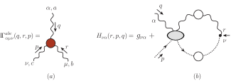
The full three-gluon vertex will be denoted by ${\rm{I}}\!\Gamma^{abc}_{\alpha\mu\nu}(q,r,p)=gf^{abc}{\rm{I}}\!\Gamma^{\alpha\mu\nu}(q,r,p)$, and is represented in Fig. 1, with $q+p+r=0$, and $g$ the gauge coupling.

Figure 1: The diagrammatic representations of the three-gluon vertex, ${\rm{I}}\!\Gamma_{\alpha\mu\nu}^{abc}(q,r,p)$, and the ghost-gluon scattering kernel, $H_{\nu\alpha}(q,r,p)$, with the respective conventions of momenta and indices.

It is convenient to decompose $\Gamma_{\alpha\mu\nu}(q,r,p)$ into two distinct pieces  Ball and Chiu (1980); Davydychev et al. (1996); Aguilar et al. (2019b),

$${\rm{I}}\!\Gamma^{\alpha\mu\nu}(q,r,p)=\Gamma_{\!{\scriptscriptstyle L}}^{\alpha\mu\nu}(q,r,p)+\Gamma_{\!{\scriptscriptstyle T}}^{\alpha\mu\nu}(q,r,p)\,,$$ (3)

where $\Gamma_{\!{\scriptscriptstyle L}}^{\alpha\mu\nu}(q,r,p)$ and $\Gamma_{\!{\scriptscriptstyle T}}^{\alpha\mu\nu}(q,r,p)$ are the “longitudinal” and “transverse” parts of the three-gluon vertex, respectively. While the former saturates the corresponding STIs [see Eq. (8)], the latter is automatically conserved when contracted by $q^{\alpha}$, $r^{\mu}$, and $p^{\nu}$, i.e., $q^{\alpha}\Gamma_{\!{\scriptscriptstyle T}}^{\alpha\mu\nu}=r^{\mu}\Gamma_{\!{\scriptscriptstyle T}}^{\alpha\mu\nu}=p^{\nu}\Gamma_{\!{\scriptscriptstyle T}}^{\alpha\mu\nu}=0$.

The tensorial decompositions of $\Gamma_{\!{\scriptscriptstyle L}}^{\alpha\mu\nu}(q,r,p)$ and $\Gamma_{\!{\scriptscriptstyle T}}^{\alpha\mu\nu}(q,r,p)$ reads

$$\Gamma_{\!{\scriptscriptstyle L}}^{\alpha\mu\nu}(q,r,p) = \sum_{i=1}^{10}X_{i}(q,r,p)\ell_{i}^{\alpha\mu\nu}\,,$$

$$\Gamma_{\!{\scriptscriptstyle T}}^{\alpha\mu\nu}(q,r,p) = \sum_{i=1}^{4}Y_{i}(q,r,p)t_{i}^{\alpha\mu\nu}\,,$$ (4)

where the explicit expressions of the basis elements $\ell_{i}^{\alpha\mu\nu}$ and $t_{i}^{\alpha\mu\nu}$ are given in Eqs. (3.4) and (3.6) of Aguilar et al. (2019a), respectively.

Another familiar quantity introduced in the studies of the three-gluon vertex is the transversally projected vertex, $\overline{\Gamma}_{\alpha\mu\nu}(q,r,p)$, defined as Eichmann et al. (2014); Huber (2020)

$$\!\!\overline{{\rm{I}}\!\Gamma}_{\alpha\mu\nu}(q,r,p)\!=\!{\rm{I}}\!\Gamma^{\alpha\!^{\prime}\mu\!^{\prime}\nu\!^{\prime}}\!(q,r,p)P_{\alpha^{\prime}\!\alpha}(q)P_{\mu^{\prime}\!\mu}(r)P_{\nu^{\prime}\!\nu}(p)\,.$$ (5)

In addition, we define the tree-level counterpart of Eq. (5),

$$\overline{\Gamma}_{\alpha\mu\nu}(q,r,p)=\Gamma_{\!0}^{\alpha\!^{\prime}\mu\!^{\prime}\nu\!^{\prime}}\!(q,r,p)P_{\alpha^{\prime}\!\alpha}(q)P_{\mu^{\prime}\!\mu}(r)P_{\nu^{\prime}\!\nu}(p),$$ (6)

where $\Gamma_{\!0}^{\alpha\!^{\prime}\mu\!^{\prime}\nu\!^{\prime}}\!(q,r,p)$ is the standard tree-level expression, given by

$$\Gamma_{\!0}^{\alpha\mu\nu}=(q-r)^{\nu}g^{\alpha\mu}+(r-p)^{\alpha}g^{\mu\nu}+(p-q)^{\mu}g^{\alpha\nu}\,;$$ (7)

it may be obtained from Eq. (3) by setting $X_{1}=X_{4}=X_{7}=1$, and zero for all other form-factors.

The STI satisfied by ${\rm{I}}\!\Gamma_{\alpha\mu\nu}(q,r,p)$ reads

$$p^{\nu}{\rm{I}}\!\Gamma_{\alpha\mu\nu}(q,r,p)=F(p^{2})[{\cal T}_{\mu\alpha}(r,p,q)-{\cal T}_{\alpha\mu}(q,p,r)]\,,$$ (8)

with

$${\cal T}_{\mu\alpha}(r,p,q):=\Delta^{-1}(r^{2})P_{\mu}^{\sigma}(r)H_{\sigma\alpha}(r,p,q)\,,$$ (9)

where $H_{\nu\mu}(q,p,q)$ denotes the ghost-gluon scattering kernel, represented diagrammatically in the panel (b) of Fig. 1. Its tensorial decomposition is given by Ball and Chiu (1980); Davydychev et al. (1996); Aguilar et al. (2019c)

$$H_{\nu\mu}(q,p,r) = g_{\nu\mu}A_{1}+q_{\mu}q_{\nu}A_{2}+r_{\mu}r_{\nu}A_{3}$$ (10)

$$+ q_{\mu}r_{\nu}A_{4}+r_{\mu}q_{\nu}A_{5}\,,$$

where we use the compact notation $A_{i}:=A_{i}(q,p,r)$.

III Nonperturbative methods

The rich kinematic structure of the three-gluon vertex makes its nonperturbative study particularly challenging. There are three main frameworks for dealing with this problem: (i) Functional methods, such as the Schwinger-Dyson equations (SDEs) Schleifenbaum et al. (2005); Huber and von Smekal (2013); Aguilar et al. (2013); Huber et al. (2012); Blum et al. (2014); Eichmann et al. (2014); Williams et al. (2016); Binosi et al. (2017) and the functional renormalization group Corell et al. (2018); Cyrol et al. (2018a, 2016); (ii) large-volume lattice simulations Parrinello et al. (1998); Boucaud et al. (1998); Cucchieri et al. (2006, 2008); Athenodorou et al. (2016); Duarte et al. (2016); Boucaud et al. (2017); Vujinovic and Mendes (2019); Aguilar et al. (2020a, 2021b); and (iii) STI-based reconstructions of the longitudinal part, $\Gamma_{\!{\scriptscriptstyle L}}^{\alpha\mu\nu}(q,r,p)$, in the spirit of the “gauge-technique” Salam (1963); Salam and Delbourgo (1964); Delbourgo and West (1977a, b).

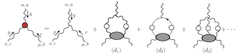
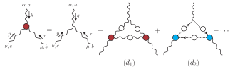
(i) Functional methods: The diagrammatic representation of the SDE that governs the evolution of the three-gluon vertex is shown in Fig. 2. The self-consistent treatment of this equation is particularly complicated, and entails its coupling to additional related equations, such as the SDEs of the gluon and ghost propagators. In practice, this task is considerably simplified by using as inputs the lattice results for $\Delta(q^{2})$ and $F(q^{2})$.

Figure 2: The SDE of the three-gluon vertex. The white (gray) circles (ellipses) indicate fully dressed propagators (kernels), while the dots indicate the omitted terms.

(ii) Lattice simulations: In this case the three-gluon vertex is accessed through the functional averaging of the quantity $\langle\widetilde{A}^{a}_{\alpha}(q)\widetilde{A}^{b}_{\mu}(r)\widetilde{A}^{c}_{\nu}(p)\rangle$, where $\widetilde{A}^{a}_{\alpha}(q)$ denotes the SU(3) gauge field. Specifically, the connected three-point function, ${\cal G}_{\alpha\mu\nu}(q,r,p)$, defined as

$${\cal G}_{\alpha\mu\nu}(q,r,p)=g\overline{{\rm{I}}\!\Gamma}_{\alpha\mu\nu}(q,r,p)\Delta(q^{2})\Delta(r^{2})\Delta(p^{2})\ ,$$ (11)

is given by $\langle\widetilde{A}^{a}_{\alpha}(q)\widetilde{A}^{b}_{\mu}(r)\widetilde{A}^{c}_{\nu}(p)\rangle=f^{abc}{\cal G}_{\alpha\mu\nu}(q,r,p)$. $\overline{{\rm{I}}\!\Gamma}_{\alpha\mu\nu}(q,r,p)$ is finally obtained after an appropriate amputation of the gluon propagators.

The typical structure of lattice “observables” is

$$L(q,p,r)=\frac{W^{\alpha\mu\nu}(q,r,p)\overline{{\rm{I}}\!\Gamma}_{\alpha\mu\nu}(q,r,p)}{\rule[0.0pt]{0.0pt}{12.80365pt}W_{\alpha\mu\nu}(q,r,p)W^{\alpha\mu\nu}(q,r,p)}\rule[0.0pt]{0.0pt}{14.22636pt}\;,$$ (12)

where the $W^{\alpha\mu\nu}(q,r,p)$ are appropriately chosen projectors Athenodorou et al. (2016); Duarte et al. (2016); Boucaud et al. (2017). In what follows we will focus our attention on two special kinematic limits involving a single momentum variable.

(a) Soft limit, corresponding to the kinematic choice

$$q\to 0\,,\quad p=-r\,,\quad\theta:=\widehat{pr}=\pi\,,$$ (13)

obtained by setting $W^{\alpha\mu\nu}(q,r,p)\to 2r^{\alpha}P^{\mu\nu}(r)$, namely

$$L_{sg}(r^{2})=\frac{\Gamma_{0}^{\alpha\mu\nu}(q,r,p)\overline{{\rm{I}}\!\Gamma}_{\alpha\mu\nu}(q,r,p)}{\rule[0.0pt]{0.0pt}{12.80365pt}\;{\Gamma_{0}^{\alpha\mu\nu}(q,r,p)\overline{\Gamma}_{\alpha\mu\nu}(q,r,p)}}\rule[0.0pt]{0.0pt}{14.22636pt}\Bigg{|}_{\begin{subarray}{c}\!\!q\to 0\\ p\to-r\end{subarray}}\,.$$ (14)

(b) Totally symmetric limit,

$$q^{2}=p^{2}=r^{2}:=s^{2}\,,\quad\theta:=\widehat{qr}=\widehat{qp}=\widehat{rp}=2\pi/3\,;$$ (15)

the corresponding $W^{\alpha\mu\nu}(q,r,p)$ and the expression for $\mathit{L}_{{sym}}(s^{2})$ may be found in Eqs. (2.18) and (2.19) of Aguilar et al. (2020a).

(iii) STI: As was first shown in Ball and Chiu (1980), the STI of Eq. (8), together with its cyclic permutation, determines the form factors $X_{i}(q,r,p)$ in terms of the kinetic part of the gluon propagator, to be denoted by $J(q^{2})$, the ghost dressing function, and three form factors of the ghost-gluon kernel.

Figure 3: A representative case of the three-gluon form factor $X_{1}(r^{2},p^{2},\theta)$ (left panel) and for $|p||r|X_{3}(r^{2},p^{2},\theta)$ (right panel) for a fixed value of the angle, $\theta:=\widehat{pr}=\pi$.

Specifically,

$$X_{1}=\frac{1}{4}[(q^{2}-r^{2})(b_{rpq}+b_{pqr}-b_{qpr}-b_{prq})]\,,$$

$$+\!2(a_{pqr}\!+\!a_{prq})\!+\!p^{2}(b_{qrp}\!+\!b_{rqp})\!+\!2(\,q\cdot p\,d_{prq}\!+\!\,r\cdot p\,d_{pqr})]\,,$$

$$X_{2}=\frac{1}{4}[2(a_{prq}-a_{pqr})-(q^{2}-r^{2})(b_{qrp}+b_{rqp})$$

$$+2(\,q\cdot p\,d_{prq}-\,r\cdot p\,d_{pqr})+p^{2}(b_{prq}-b_{pqr}+b_{qpr}-b_{rpq})]\,,$$

$$X_{3}=\frac{1}{q^{2}-r^{2}}[a_{rpq}-a_{qpr}+r\cdot p\,d_{qpr}-q\cdot p\,d_{rpq}]\,,$$

$$X_{10}=-\frac{1}{2}[b_{qrp}+b_{rpq}+b_{pqr}-b_{qpr}-b_{rqp}-b_{prq}],$$ (16)

where we introduced the following compact notation

$$a_{qrp}:= F(r)J(p)A_{1}(p,r,q)\,,$$

$$b_{qrp}:= F(r)J(p)A_{3}(p,r,q)\,,$$

$$d_{qrp}:= F(r)J(p)[A_{4}(p,r,q)-A_{3}(p,r,q)]\,.$$ (17)

Due to the Bose symmetry of the three-gluon vertex, the remaining six $X_{i}$ may be computed by permuting the arguments appropriately (see Eq. (3.8) of Aguilar et al. (2019a)).

It is important to emphasize that in the original work of Ball and Chiu (1980) the kinetic term of the gluon propagator was defined as $\Delta^{-1}(q^{2})=q^{2}J(q^{2})$, while in the nonperturbative generalization presented in Aguilar et al. (2019a) we have $\Delta^{-1}(q^{2})=q^{2}J(q^{2})+m^{2}(q^{2})$, where $m^{2}(q^{2})$ is the running gluon mass Cornwall (1982); Aguilar et al. (2008); Binosi and Papavassiliou (2009); Cornwall (1982); Aguilar et al. (2008); Roberts (2020).

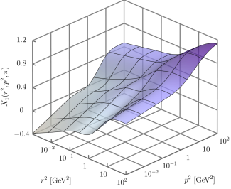
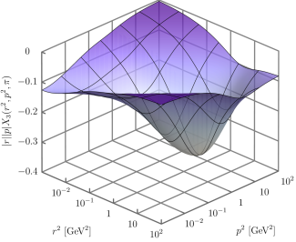
Two representative results for the form factors $X_{1}(r^{2},p^{2},\theta$) and $|q||r|X_{3}(r^{2},p^{2},\theta$), obtained with Eq. (16), are shown on Fig. 3. In this figure we present both form factors as a function of the two momenta $p^{2}$ and $r^{2}$ when the angle between these two momenta is fixed at the value $\theta=\pi$.

Clearly, one can see that $X_{1}(r^{2},p^{2},\theta)$ has a completely nontrivial structure, which persists for general values of the angle. Evidently, the most striking feature of this result is the reduction of the size of $X_{1}(r^{2},p^{2},\theta)$ with respect to its tree-level value (unity); this effect is known in the literature as “infrared suppression” Aguilar et al. (2014); Athenodorou et al. (2016); Boucaud et al. (2017); Blum et al. (2015); Corell et al. (2018); Huber (2020); Aguilar et al. (2019a).

Let us also point out that the projection of the three gluon vertex in the totally symmetric limit, defined in Eq. (15), can be written as Aguilar et al. (2019a)

$$\mathit{L}_{{sym}}(s^{2}) = X_{1}(s^{2})-\frac{s^{2}}{2}X_{3}(s^{2})$$ (18)

$$+ \frac{s^{4}}{4}Y_{1}(s^{2})-\frac{s^{2}}{2}Y_{4}(s^{2})\,.$$

Figure 4: The projection of the three-gluon vertex in the soft gluon, $\mathit{L}_{{sg}}(r^{2})$ (left) and in the symmetric, $\mathit{L}_{{sym}}(s^{2})$, (right) kinematic configurations obtained from lattice QCD of Athenodorou et al. (2016); Boucaud et al. (2017); Aguilar et al. (2021b) (solid circles) and from the SDE-STIs approach (magenta continuous curve) Aguilar et al. (2021b).

Figure 5: Left panel: The unquenched $\mathit{L}_{{sg}}(r^{2})$ (left) and $\mathit{L}_{{sym}}(s^{2})$ (right) obtained from lattice QCD with $N_{f}=2+1$ dynamical quarks Aguilar et al. (2020a), and from the SDE-STI approach (magenta continuous curve).

On other hand, for the case of the soft limit configuration of Eq. (13), the expression for $\mathit{L}_{{sg}}(r^{2})$ is given by

$$\mathit{L}_{{sg}}(r^{2})=X_{1}(r^{2},r^{2},\pi)-r^{2}X_{3}(r^{2},r^{2},\pi)\,\,;$$ (19)

note that the result is free of transverse form factors $Y_{i}$.

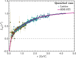
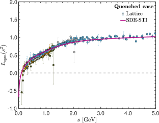
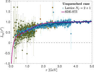
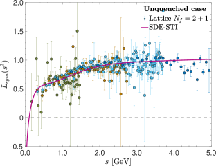
Notice that the soft gluon kinematic limit of $X_{1}$ and $X_{3}$ corresponds to the curves that lie on the diagonal “slice” of the 3D plots of Fig. 3 where $p^{2}=r^{2}$. In the left panel of Fig. 4 we show a comparison of the $\mathit{L}_{{sg}}(r^{2})$ computed using the SDE-STI approach (magenta continuous curve) and a combination of the lattice data of Athenodorou et al. (2016); Boucaud et al. (2017); Aguilar et al. (2021b) (solid circles), for the case of quenched QCD. It is clear that both methods corroborate the infrared suppression of the three-gluon vertex. In the right panel we show the results for $\mathit{L}_{{sym}}(s^{2})$, obtained when we set $Y_{i}=0$ in Eq. (18). Once again the coincidence with the lattice data is rather notable, and the presence of the steep decline in the infrared is visible in both approaches. In addition, the same pattern (suppression and zero crossing) persists qualitatively unaltered when $N_{f}=2+1$ dynamical quarks are added Aguilar et al. (2020a), as can be clearly seen in Fig. 5.

IV Infrared suppression

One of the most remarkable nonperturbative features of the three-gluon vertex in the Landau gauge is its infrared suppression, as established clearly in the results of the previous section. Thus, form factors such as $X_{1}$, $X_{4}$, and $X_{7}$, which, due to renormalization, acquire their tree level value (unity) at $4.3$ GeV, reduce their size to half at around $1$ GeV. This tendency culminates with a characteristic reversal of the sign, known as “zero crossing” Aguilar et al. (2014); Eichmann et al. (2014); Blum et al. (2014); Vujinovic et al. (2014); Athenodorou et al. (2016); Boucaud et al. (2017), followed by a logarithmic divergence of the corresponding form factor at the origin.

This type of behavior is in sharp contradistinction to what happens with the other vertices of the theory that have been explored so far, such as the quark-gluon or the ghost-gluon vertex. Indeed, as one can see in Fig. 6, the analogous form factors display a clear enhancement for the same range of intermediate and infrared momenta.

Figure 6: The behavior of the form factors, $L_{1}^{sg}(q^{2})$, $B_{1}^{sg}(q^{2})$, and $\mathit{L}_{{sg}}(q^{2})$ associated with the classical tensor structures of the quark-gluon (green dotted), ghost-gluon (blue dashed) and three-gluon (magenta continuous) vertices, respectively, in the soft gluon limit.

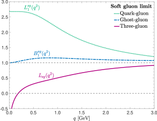
From the theoretical point of view, this particular feature of the three-gluon vertex hinges on the subtle interplay between dynamical effects originating from the two-point sector of the theory Roberts and Williams (1994); Alkofer and von Smekal (2001); Fischer (2006); Cloet and Roberts (2014); Aguilar et al. (2016); Binosi et al. (2015). This may be understood at the level of the one-loop dressed version of the SDE in Fig.  2, which is shown in Fig.  7. The crucial theoretical ingredient is that, whereas the gluon acquires dynamically an effective mass, the ghost remains massless even nonperturbatively. As a result, the loops of the three-gluon vertex containing gluons (such as the ($d_{1}$) in Fig.  7) give rise to “protected” logarithms, because the effective gluon mass $m$ acts as an infrared regulator. Instead, loops containing ghosts (such as the ($d_{2}$) in Fig. 7) produce “unprotected” logarithms, which diverge at the origin Aguilar et al. (2014).

In the simplified kinematic circumstances where only a single representative momentum $q^{2}$ is considered, a basic model describing qualitatively the resulting dynamics is given by

$$L(q^{2})=b_{0}+b_{\rm gl}\ln\left(\frac{q^{2}+m^{2}}{\Lambda^{2}}\right)+b_{\rm gh}\ln\left(\frac{q^{2}}{\Lambda^{2}}\right)\,,$$ (20)

where $L(q^{2})$ denotes the particular combination of form factors, such that, at tree-level, $L_{0}(q^{2})=1$, and $b_{0}$, $b_{\rm gl}$, and $b_{\rm gh}$ are positive constants.

It is clear that, as $q\to 0$, the term with the unprotected logarithm will dominate over the others, forcing $L(q^{2})$ to reverse its sign (zero crossing), and finally diverge, $L(0)\to-\infty$. Because, in practice, $b_{\rm gl}$ is about one order of magnitude larger than $b_{\rm gh}$, the point where the unprotected logarithm overtakes the protected one is rather deep in the infrared, and the location of the zero-crossing is at about $120$ MeV. Thus, in the intermediate region of momenta, which is typically relevant for the onset of nonperturbative dynamics, we have $L(q^{2})<1$; this effect is known as the infrared suppression of the three-gluon vertex.

Figure 7: The SDE of the three-gluon vertex at the one-loop dressed level. The white (red and blue) circles indicate fully dressed propagators (vertices). The diagrams $(d_{1})$ and $(d_{2})$ are the gluon and the ghost triangle contributions entering in the skeleton expansion of three-gluon vertex.

V Phenomenology

In this section we discuss two representative phenomenological applications, where the infrared suppression of the corresponding form factors plays a crucial role.

V.1 Effective couplings

A typical quantity employed in a variety of phenomenological applications is the effective charge, defined as a special renormalization-group invariant combination of propagators and vertex form factors. In the case of the three-gluon vertex in the soft-gluon limit, the corresponding charge, to be denoted by ${\alpha}_{\rm{3g}}(q^{2})$, is defined as Alkofer et al. (2005); Fischer (2006); Athenodorou et al. (2016); Fu et al. (2020); Aguilar et al. (2021c)

$${\alpha}_{\rm{3g}}(q^{2})={\alpha}_{s}(\mu^{2})\mathit{L}_{{sg}}^{2}(q^{2})\mathcal{Z}^{3}(q^{2})\,,$$ (21)

with $\mathcal{Z}(q^{2})$ defined in Eq. (1).

It is natural to expect that the infrared suppression of $\mathit{L}_{{sg}}^{2}(q^{2})$ will affect the shape and size of ${\alpha}_{\rm{3g}}(q^{2})$. In order to meaningfully quantify this suppression, we compare ${\alpha}_{\rm{3g}}(q^{2})$ with the corresponding quantity defined from the ghost-gluon vertex, to be denoted ${\alpha}_{\rm{cg}}(q^{2})$, namely (see, e.g.,  Alkofer et al. (2005); Fischer (2006); Aguilar et al. (2009))

$${\alpha}_{\rm{cg}}(q^{2})={\alpha}_{s}(\mu^{2})B_{1\,sg}^{2}(q^{2})F^{2}(q^{2})\mathcal{Z}(q^{2})\,,$$ (22)

where $B_{1\,sg}(q^{2})$ is the ghost-gluon form factor introduced in Fig. 6.

Figure 8: The comparison of the effective couplings, ${\alpha}_{\rm{cg}}(q^{2})$ (blue dashed line) and ${\alpha}_{\rm{3g}}(q^{2})$ (magenta continuous curve).

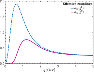
It is important to mention that both effective couplings are computed in the same renormalization scheme, namely the Taylor scheme Boucaud et al. (2009, 2011); von Smekal et al. (2009) where we have fixed that ${\alpha}_{s}(\mu)=0.244$, at $\mu=4.3$ GeV (for more details see Aguilar et al. (2021c)).

The comparison of the two effective charges is displayed in Fig. 8. One clearly sees that, as the momentum $q$ decreases, ${\alpha}_{\rm{3g}}(q^{2})$ (magenta continuous) becomes considerably smaller than ${\alpha}_{\rm{cg}}(q^{2})$ (blue dashed line). The suppression of ${\alpha}_{\rm{3g}}(q^{2})$, located in the region below $2$ GeV is consistent with previous finding Huber and von Smekal (2013); Blum et al. (2014); Williams (2015); Cyrol et al. (2016, 2018a); Aguilar et al. (2020b), and its origin is exclusively associated with the suppression of the $\mathit{L}_{{sg}}(q^{2})$.

V.2 Pseudoscalar glueball

The dynamical generation of a mass gap in pure-gauge QCD is intimately connected with the attendant appearance of glueball bound-states Cornwall (1982). The rich glueball spectrum, and related fundamental properties, has been obtained by means of detailed lattice simulations, see e.g.,  Morningstar and Peardon (1999); Bali et al. (1993); McNeile (2009); Chen et al. (2006); Athenodorou and Teper (2020). Evidently, these results serve as valuable benchmarks in the ongoing effort of continuum bound-state methods to reach an intuitive understanding of the underlying dynamics Dudal et al. (2011); Meyers and Swanson (2013); Souza et al. (2020); Huber et al. (2021).

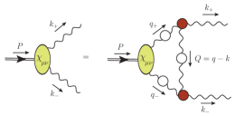
In this context, the $J^{PC}=0^{-+}$ glueball represents the simplest case, because the pertinent Bethe-Salpeter equation possesses a single dynamical kernel, which essentially describes the four-gluon scattering process. The lowest-order contribution of this kernel is shown in Fig. 9; evidently, the three-gluon vertex constitutes one of its central ingredients Souza et al. (2020).

Moreover, the corresponding amplitude involves only one scalar function, namely

$$\chi_{\mu\nu}(k_{+},k_{-})=\epsilon_{\mu\nu\alpha\beta}k^{\alpha}P^{\beta}\mathcal{F}(k;P)\,,$$ (23)

simplifying considerably the treatment of this problem.

Figure 9: The diagrammatic representation of the Bethe-Salpeter equation for the pseudoscalar glueball with total momentum $P$, and $\ell_{\pm}:=P/2\pm\ell$, for $\ell=k,q$ .

It turns out that the infrared suppression of the three-gluon vertex, and the overall attenuation of the interaction strength that it induces is instrumental for the formation of the pseudoscalar glueball state, with a mass compatible with that obtained from the lattice Souza et al. (2020).

Let us finally mention that the need for a considerable suppression has also been established in studies of hybrid states by means of Faddeev equations Xu et al. (2019).

VI Conclusions

In this presentation we have reviewed some of the most characteristic nonpertubative features of the three-gluon vertex, unraveled by the ongoing synergy of a multitude of techniques and approaches, such as functional methods, lattice simulations, and STI-based constructions.

We have focused on the interplay between the dynamics of the three-gluon vertex and the Landau-gauge two-point sector of the theory. In particular, as has been argued in Sec. IV, the characteristic infrared suppression displayed by the main form factors of the three-gluon vertex is tightly interlocked with the mass generating pattern established in the gauge sector of QCD.

There is an additional key aspect of the three-gluon vertex, which is worth mentioning, albeit in passing. In particular, the three-gluon vertex develops longitudinally coupled bound state massless poles, which trigger the well-known Schwinger mechanism Schwinger (1962a, b), endowing the gluons with a dynamical mass scale Aguilar et al. (2008); Binosi and Papavassiliou (2009, 2009). Due to their special kinematic properties, these poles decouple from the transversally projected vertex $\overline{\Gamma}_{\alpha\mu\nu}(q,r,p)$ [see Eq. (5)], which enters in the lattice quantities defined according to Eq. (12). Consequently, these dynamically produced poles do not induce divergences in the results displayed in Fig. 4 and Fig. 5. Nonetheless, as has been recently demonstrated in Aguilar et al. (2021a), the massless poles leave smoking-gun signals of their presence, by inducing finite displacements to the non-Abelian Ward identity satisfied by the pole-free part of the three-gluon vertex. Quite interestingly, this displacement is identical to the Bethe-Salpeter amplitude that controls the dynamical formation of the massless poles Aguilar et al. (2012); Ibañez and Papavassiliou (2013); Aguilar et al. (2018); Binosi and Papavassiliou (2018), thus establishing a powerful constraint on the entire mass generating mechanism put forth in a series of works (see Aguilar et al. (2021a) and references therein).

It would be clearly important to continue the research activity surrounding the three-gluon vertex in the future. In this context, a major challenge for functional methods is the extension of the results for this vertex from space-like to time-like momenta. Such information will be particularly important, both from the theoretical as well as the phenomenological point of view. The methods and techniques developed in Cyrol et al. (2018b); Horak et al. (2020, 2021a, 2021b) may be decisive for making progress with this demanding endeavor.

References

- Marciano and Pagels (1978) W. J. Marciano and H. Pagels, Phys. Rept. 36, 137 (1978).
- Ball and Chiu (1980) J. S. Ball and T.-W. Chiu, Phys. Rev. D 22, 2550 (1980), [Erratum: Phys.Rev.D 23, 3085 (1981)].
- Davydychev et al. (1996) A. I. Davydychev, P. Osland, and O. Tarasov, Phys. Rev. D 54, 4087 (1996), [Erratum: Phys.Rev.D 59, 109901 (1999)].
- Gross and Wilczek (1973) D. J. Gross and F. Wilczek, Phys. Rev. Lett. 30, 1343 (1973).
- Politzer (1973) H. D. Politzer, Phys. Rev. Lett. 30, 1346 (1973).
- Alkofer et al. (2005) R. Alkofer, C. S. Fischer, and F. J. Llanes-Estrada, Phys. Lett. B 611, 279 (2005), [Erratum: Phys.Lett.B 670, 460–461 (2009)].
- Huber et al. (2012) M. Q. Huber, A. Maas, and L. von Smekal, J. High Energy Phys. 11, 035 (2012).
- Pelaez et al. (2013) M. Pelaez, M. Tissier, and N. Wschebor, Phys. Rev. D88, 125003 (2013).
- Aguilar et al. (2014) A. C. Aguilar, D. Binosi, D. Ibañez, and J. Papavassiliou, Phys. Rev. D89, 085008 (2014).
- Blum et al. (2014) A. Blum, M. Q. Huber, M. Mitter, and L. von Smekal, Phys. Rev. D89, 061703 (2014).
- Eichmann et al. (2014) G. Eichmann, R. Williams, R. Alkofer, and M. Vujinovic, Phys. Rev. D89, 105014 (2014).
- Mitter et al. (2015) M. Mitter, J. M. Pawlowski, and N. Strodthoff, Phys. Rev. D91, 054035 (2015).
- Williams et al. (2016) R. Williams, C. S. Fischer, and W. Heupel, Phys. Rev. D93, 034026 (2016).
- Blum et al. (2015) A. L. Blum, R. Alkofer, M. Q. Huber, and A. Windisch, Acta Phys. Polon. Supp. 8, 321 (2015).
- Cyrol et al. (2016) A. K. Cyrol, L. Fister, M. Mitter, J. M. Pawlowski, and N. Strodthoff, Phys. Rev. D94, 054005 (2016).
- Corell et al. (2018) L. Corell, A. K. Cyrol, M. Mitter, J. M. Pawlowski, and N. Strodthoff, SciPost Phys. 5, 066 (2018).
- Boucaud et al. (2017) P. Boucaud, F. De Soto, J. Rodríguez-Quintero, and S. Zafeiropoulos, Phys. Rev. D95, 114503 (2017).
- Huber (2020) M. Q. Huber, Phys. Rept. 879, 1 (2020).
- Aguilar et al. (2019a) A. C. Aguilar, M. N. Ferreira, C. T. Figueiredo, and J. Papavassiliou, Phys. Rev. D99, 094010 (2019a).
- Aguilar et al. (2020a) A. C. Aguilar, F. De Soto, M. N. Ferreira, J. Papavassiliou, J. Rodríguez-Quintero, and S. Zafeiropoulos, Eur. Phys. J. C 80, 154 (2020a).
- Aguilar et al. (2019b) A. C. Aguilar, M. N. Ferreira, C. T. Figueiredo, and J. Papavassiliou, Phys. Rev. D 100, 094039 (2019b).
- Parrinello (1994) C. Parrinello, Phys. Rev. D50, R4247 (1994).
- Alles et al. (1997) B. Alles, D. Henty, H. Panagopoulos, C. Parrinello, C. Pittori, and D. G. Richards, Nucl. Phys. B502, 325 (1997).
- Parrinello et al. (1998) C. Parrinello, D. Richards, B. Alles, H. Panagopoulos, and C. Pittori (UKQCD), Nucl. Phys. B Proc. Suppl. 63, 245 (1998).
- Boucaud et al. (1998) P. Boucaud, J. P. Leroy, J. Micheli, O. Pene, and C. Roiesnel, J. High Energy Phys. 10, 017 (1998).
- Cucchieri et al. (2006) A. Cucchieri, A. Maas, and T. Mendes, Phys. Rev. D74, 014503 (2006).
- Cucchieri et al. (2008) A. Cucchieri, A. Maas, and T. Mendes, Phys. Rev. D77, 094510 (2008).
- Athenodorou et al. (2016) A. Athenodorou, D. Binosi, P. Boucaud, F. De Soto, J. Papavassiliou, J. Rodriguez-Quintero, and S. Zafeiropoulos, Phys. Lett. B761, 444 (2016).
- Duarte et al. (2016) A. G. Duarte, O. Oliveira, and P. J. Silva, Phys. Rev. D94, 074502 (2016).
- Vujinovic and Mendes (2019) M. Vujinovic and T. Mendes, Phys. Rev. D99, 034501 (2019).
- Cornwall (1982) J. M. Cornwall, Phys. Rev. D 26, 1453 (1982).
- Alkofer et al. (2009) R. Alkofer, M. Q. Huber, and K. Schwenzer, Eur. Phys. J. C 62, 761 (2009).
- Alkofer et al. (2010) R. Alkofer, M. Q. Huber, and K. Schwenzer, Phys. Rev. D 81, 105010 (2010).
- Aguilar et al. (2008) A. C. Aguilar, D. Binosi, and J. Papavassiliou, Phys. Rev. D78, 025010 (2008).
- Vujinovic et al. (2014) M. Vujinovic, R. Alkofer, G. Eichmann, and R. Williams, Acta Phys. Polon. Supp. 7, 607 (2014).
- Aguilar et al. (2021a) A. C. Aguilar, M. N. Ferreira, and J. Papavassiliou, [arXiv:2111.09431 [hep-ph]] .
- Eichmann et al. (2021) G. Eichmann, J. M. Pawlowski, and J. M. Silva, Phys. Rev. D 104, 114016 (2021).
- Eichmann and Pawlowski (2021) G. Eichmann and J. M. Pawlowski, in [arXiv:2112.08058 [hep-ph]] .
- Meyers and Swanson (2013) J. Meyers and E. S. Swanson, Phys. Rev. D87, 036009 (2013).
- Souza et al. (2020) E. V. Souza, M. N. Ferreira, A. C. Aguilar, J. Papavassiliou, C. D. Roberts, and S.-S. Xu, Eur. Phys. J. A 56, 25 (2020).
- Huber et al. (2021) M. Q. Huber, C. S. Fischer, and H. Sanchis-Alepuz, Eur. Phys. J. C 81, 1083 (2021).
- Aguilar et al. (2019c) A. C. Aguilar, M. N. Ferreira, C. T. Figueiredo, and J. Papavassiliou, Phys. Rev. D99, 034026 (2019c).
- Schleifenbaum et al. (2005) W. Schleifenbaum, A. Maas, J. Wambach, and R. Alkofer, Phys. Rev. D 72, 014017 (2005).
- Huber and von Smekal (2013) M. Q. Huber and L. von Smekal, J. High Energy Phys. 04, 149 (2013).
- Aguilar et al. (2013) A. C. Aguilar, D. Ibañez, and J. Papavassiliou, Phys. Rev. D87, 114020 (2013).
- Binosi et al. (2017) D. Binosi, L. Chang, J. Papavassiliou, S.-X. Qin, and C. D. Roberts, Phys. Rev. D95, 031501 (2017).
- Cyrol et al. (2018a) A. K. Cyrol, M. Mitter, J. M. Pawlowski, and N. Strodthoff, Phys. Rev. D97, 054006 (2018a).
- Aguilar et al. (2021b) A. C. Aguilar, F. De Soto, M. N. Ferreira, J. Papavassiliou, and J. Rodríguez-Quintero, Phys. Lett. B 818, 136352 (2021b).
- Salam (1963) A. Salam, Phys. Rev. 130, 1287 (1963).
- Salam and Delbourgo (1964) A. Salam and R. Delbourgo, Phys. Rev. 135, B1398 (1964).
- Delbourgo and West (1977a) R. Delbourgo and P. C. West, J. Phys. A 10, 1049 (1977a).
- Delbourgo and West (1977b) R. Delbourgo and P. C. West, Phys. Lett. B 72, 96 (1977b).
- Binosi and Papavassiliou (2009) D. Binosi and J. Papavassiliou, Phys. Rept. 479, 1 (2009).
- Roberts (2020) C. D. Roberts, Symmetry 12, 1468 (2020).
- Roberts and Williams (1994) C. D. Roberts and A. G. Williams, Prog. Part. Nucl. Phys. 33, 477 (1994).
- Alkofer and von Smekal (2001) R. Alkofer and L. von Smekal, Phys. Rept. 353, 281 (2001).
- Fischer (2006) C. S. Fischer, J. Phys. G 32, R253 (2006).
- Cloet and Roberts (2014) I. C. Cloet and C. D. Roberts, Prog. Part. Nucl. Phys. 77, 1 (2014).
- Aguilar et al. (2016) A. C. Aguilar, D. Binosi, and J. Papavassiliou, Front. Phys.(Beijing) 11, 111203 (2016).
- Binosi et al. (2015) D. Binosi, L. Chang, J. Papavassiliou, and C. D. Roberts, Phys. Lett. B742, 183 (2015).
- Fu et al. (2020) W.-j. Fu, J. M. Pawlowski, and F. Rennecke, Phys. Rev. D 101, 054032 (2020).
- Aguilar et al. (2021c) A. C. Aguilar, C. O. Ambrósio, F. De Soto, M. N. Ferreira, B. M. Oliveira, J. Papavassiliou, and J. Rodríguez-Quintero, Phys. Rev. D 104, 054028 (2021c).
- Aguilar et al. (2009) A. C. Aguilar, D. Binosi, J. Papavassiliou, and J. Rodriguez-Quintero, Phys. Rev. D80, 085018 (2009).
- Boucaud et al. (2009) P. Boucaud, F. De Soto, J. Leroy, A. Le Yaouanc, J. Micheli, et al., Phys. Rev. D79, 014508 (2009).
- Boucaud et al. (2011) P. Boucaud, D. Dudal, J. Leroy, O. Pene, and J. Rodriguez-Quintero, J. High Energy Phys. 12, 018 (2011).
- von Smekal et al. (2009) L. von Smekal, K. Maltman, and A. Sternbeck, Phys. Lett. B 681, 336 (2009).
- Williams (2015) R. Williams, Eur. Phys. J. A51, 57 (2015).
- Aguilar et al. (2020b) A. C. Aguilar, M. N. Ferreira, and J. Papavassiliou, Eur. Phys. J. C 80, 887 (2020b).
- Morningstar and Peardon (1999) C. J. Morningstar and M. J. Peardon, Phys. Rev. D60, 034509 (1999).
- Bali et al. (1993) G. S. Bali, K. Schilling, A. Hulsebos, A. C. Irving, C. Michael, and P. W. Stephenson (UKQCD), Phys. Lett. B 309, 378 (1993).
- McNeile (2009) C. McNeile, Nucl. Phys. B Proc. Suppl. 186, 264 (2009).
- Chen et al. (2006) Y. Chen et al., Phys. Rev. D 73, 014516 (2006).
- Athenodorou and Teper (2020) A. Athenodorou and M. Teper, JHEP 11, 172 (2020).
- Dudal et al. (2011) D. Dudal, M. S. Guimaraes, and S. P. Sorella, Phys. Rev. Lett. 106, 062003 (2011).
- Xu et al. (2019) S.-S. Xu, Z.-F. Cui, L. Chang, J. Papavassiliou, C. D. Roberts, and H.-S. Zong, Eur. Phys. J. A55, 113 (2019).
- Schwinger (1962a) J. S. Schwinger, Phys. Rev. 125, 397 (1962a).
- Schwinger (1962b) J. S. Schwinger, Phys. Rev. 128, 2425 (1962b).
- Aguilar et al. (2012) A. C. Aguilar, D. Ibanez, V. Mathieu, and J. Papavassiliou, Phys. Rev. D85, 014018 (2012).
- Ibañez and Papavassiliou (2013) D. Ibañez and J. Papavassiliou, Phys. Rev. D87, 034008 (2013).
- Aguilar et al. (2018) A. C. Aguilar, D. Binosi, C. T. Figueiredo, and J. Papavassiliou, Eur. Phys. J. C78, 181 (2018).
- Binosi and Papavassiliou (2018) D. Binosi and J. Papavassiliou, Phys. Rev. D97, 054029 (2018).
- Cyrol et al. (2018b) A. K. Cyrol, J. M. Pawlowski, A. Rothkopf, and N. Wink, SciPost Phys. 5, 065 (2018b).
- Horak et al. (2020) J. Horak, J. M. Pawlowski, and N. Wink, Phys. Rev. D 102, 125016 (2020).
- Horak et al. (2021a) J. Horak, J. Papavassiliou, J. M. Pawlowski, and N. Wink, Phys. Rev. D 104, 074017 (2021a).
- Horak et al. (2021b) J. Horak, J. M. Pawlowski, J. Rodríguez-Quintero, J. Turnwald, J. M. Urban, N. Wink, and S. Zafeiropoulos, arXiv:2107.13464 [hep-ph]].b.