Fluid infiltration of a heterogeneous medium: A stochastic model

Abstract

Fluid infiltration of a permeable brick in contact with a pressurized reservoir of fluid is considered. A stochastic model, informed by Darcy’s law and the incompressibility of the fluid, shows how the heterogeneity of the permeability field affects the time evolution of the fluid infiltration. In particular, the cause of “anomalous” (non-Darcian) advance of a plume is determined. The model is applied to bricks that are linear arrays of Sierpinski carpets. These calculated results are compared to experimental results available in the literature, to verify the model and method.

I Introduction

Fluid flow through heterogeneous media is a topic of continuing scientific interest with important technological applications and implications. The particular phenomenon considered here is fluid infiltration of a permeable brick due to contact, at one end of the brick, with a pressurized reservoir of the fluid. Not only the heterogeneity of the brick composition but also the confining surfaces of the brick affect the rate of advance of the fluid into the brick.

The operative equation for this is Darcy’s law, which relates the pressure gradient in the fluid to the flow rate. The local version is

$$\mathbf{q}(\mathbf{r})=-\frac{\kappa(\mathbf{r})}{\mu}\mathbf{\mathbf{\nabla}}p(\mathbf{r})$$ (1)

where $\mathbf{q}(\mathbf{r})$ is the volumetric flow rate at position $\mathbf{r}$ within the brick, $p(\mathbf{r})$ is the fluid pressure, $\kappa(\mathbf{r})$ is the permeability, and $\mu$ is the viscosity of the fluid. [Note that other driving forces, such as gravity and capillarity, are not considered here.] The incompressibility of the fluid produces the additional equation

$$\mathbf{\mathbf{\nabla}}\cdot\mathbf{q}(\mathbf{r})=0$$ (2)

which equivalently (for the purposes of this paper) means there are no fluid sources or sinks except at the boundaries of the fluid plume.

A realistic model for fluid advance in a one-dimensional (1D) homogeneous brick is illustrated in Fig. 1.

Figure 1: Fluid pressure profiles, at successive times $t$, within a plume infiltrating a one-dimensional, homogeneous brick. The fluid pressure at the reservoir/brick interface (represented by the vertical line) remains constant as the plume advances left to right, while the pressure gradient within the plume remains linear. In effect, the “steady-state” condition holds continuously as the plume grows.

It shows the fluid pressure profile in the brick, at three successive times $t_{1}<t_{2}<t_{3}$. As the fluid is incompressible, the steady-state condition Eq. (2) holds continuously so that the pressure profile remains linear, with slope (gradient) $-p(0)/x(t)$ where $p(0)$ is the constant fluid pressure at the reservoir/brick interface, and $x(t)$ is the extent of the fluid advance into the brick at time $t$. The flow rate into the brick at time $t$ is $d\left[x(t)\right]/dt$. Then Darcy’s law implies

$$\frac{d}{dt}x(t)=\frac{\kappa}{\mu}\>\frac{p(0)}{x(t)}$$ (3)

which has the solution

$$x(t)=\left[2\,\frac{\kappa}{\mu}\>p(0)\right]^{1/2}t^{1/2}.$$ (4)

It bears comment that the value of the reservoir pressure $p(0)$ has no effect on the time exponent.

This model is the motivation for what follows. Most importantly, it relies on the continuous application of the steady-state condition as the fluid advances.

To apply the model to 2D and 3D heterogeneous bricks, then, it is necessary to ensure a steady-state pressure field $\left\{p(\mathbf{r})\right\}$ in the infiltrated fluid at time $t$. This is done by the Walker Diffusion Method (WDM), which for this purpose effectively solves the large set of coupled equations that are the discretized version of the steady-state equation

$$\nabla\cdot\left[\frac{\kappa(\mathbf{r})}{\mu}\mathbf{\nabla}p(\mathbf{r})\right]=0$$ (5)

with boundary conditions of constant pressure at the reservoir/brick interface, and zero pressure ahead of the fluid front. Such calculations performed for a succession of times $t$ gives the time evolution of the fluid infiltration (the size of the plume).

Of course the pressure field and fluid advance are influenced by the domain (referring to regions of homogeneous permeability) geometry and composition of the brick. It is generally believed that the time evolution is a power law, with an exponent $\gamma$ that reflects the physical character of the portion of the brick saturated by the fluid. In cases that a brick contains regions of different permeability, the exponent value may be calculated by the WDM (via the pressure field calculations), as demonstrated in this paper. Indeed, the primary goal for this model is to connect $\gamma$ values with brick domain geometries, so that experimentally obtained values can be interpreted.

The WDM is described briefly in the following section; subsequent sections develop the fluid infiltration model and apply it to illustrative bricks. A final section very briefly summarizes the general results that are obtained.

II Walker Diffusion Method

The WDM [PRE99, ,PRE02, ] exploits the isomorphism between the transport equations [e.g., Eq. (1)] and the diffusion equation for a collection of noninteracting random walkers in the presence of a driving force,

$$\mathbf{J}(\mathbf{r})=-D(\mathbf{r})\,\rho(\mathbf{r})\mathbf{\,\nabla}\phi(\mathbf{r})$$ (6)

where $D(\mathbf{r})$ and $\rho(\mathbf{r})$ are the local walker diffusion coefficient and local walker density, respectively. In this application of the WDM, the product $D(\mathbf{r})\,\rho(\mathbf{r})$ is identified with the local permeability $\kappa(\mathbf{r})$. Specifically, $D(\mathbf{r})\,\rho^{0}(\mathbf{r})=\kappa(\mathbf{r})/\mu$, where $\rho^{0}(\mathbf{r})$ is the equilibrium walker density (meaning, in the absence of a driving force). So that the walker trajectories fully reflect the domain geometry the local diffusion coefficient $D(\mathbf{r})$ is everywhere set equal to $1$.

The domains [distinguished by different values of $\kappa(\mathbf{r})/\mu$] of the medium thus correspond to distinct populations of walkers, where the equilibrium walker density of a population is given by the value $\kappa(\mathbf{r})/\mu$. The principle of detailed balance ensures that the equilibrium population densities are maintained, and so provides the following rule for walker diffusion over a digitized (pixelated) multi-domain material: a walker at site (or pixel) $i$ attempts a move to a randomly chosen adjacent site $j$ during the time interval $\tau=(4d)^{-1}$, where $d$ is the Euclidean dimension of the space; this move is successful with probability $p_{i\rightarrow j}=\kappa_{j}/(\kappa_{i}+\kappa_{j})$, where $\kappa_{i}$ and $\kappa_{j}$ are the permeabilities of sites $i$ and $j$, respectively. (Note this is “blind ant” behavior.) The path of a walker thus reflects the permeability and morphology of the domains that are encountered.

For the purposes of this paper, a key component of the WDM [PRE02, ] is the concept of a “residence time” associated with each site visited by a walker. As the walker diffuses over the permeable medium, the time required for a move from site $i$ (which may be many multiples of $\tau$) is accrued to the residence time $t_{i}$. Note that at equilibrium (i.e., in the absence of a driving force), a single diffusing walker will occupy the sites of the system in proportion to the corresponding transport coefficients $\kappa(\mathbf{r})/\mu$; thus, in the limit of infinite time, the equilibrium walker density at site $i$ is given by

$$\rho_{i}^{0}=\frac{\kappa_{i}}{\mu}=\frac{t_{i}}{\left\langle t_{k}\right\rangle}\frac{\left\langle\kappa_{k}\right\rangle}{\mu}$$ (7)

where the averages implied by the angle brackets are taken over all visited sites $k$.

These walker densities are altered when a potential gradient is created by injecting numerous walkers into the system at one boundary or point (the “source”), and removing them at another (the “sink”). The steady-state walker density at site $i$ is then

$$\rho_{i}=\frac{t_{i}}{\left\langle t_{k}\right\rangle}\frac{\left\langle\kappa_{k}\right\rangle}{\mu}$$ (8)

where the residence time $t_{i}$ accounts for visits by all walkers to site $i$, and the averages implied by the angle brackets are taken over all visited sites $k$. As derived in Ref. [PRE02, ], the (dimensionless) potential at site $i$ is

$$\phi_{i}=\frac{\rho_{i}}{\rho_{i}^{0}}=\frac{t_{i}}{\left\langle t_{k}\right\rangle}\frac{\left\langle\kappa_{k}\right\rangle}{\kappa_{i}}$$ (9)

and the walker flux $J_{i\rightarrow j}$ between adjacent sites is

$$J_{i\rightarrow j}=\frac{1}{\mu}\>\frac{2\,\kappa_{i}\,\kappa_{j}}{\kappa_{i}+\kappa_{j}}\left(\phi_{i}-\phi_{j}\right).$$ (10)

In this paper, the driving force for fluid flow is the fluid pressure gradient, so the potential field $\left\{\phi_{i}\right\}$ corresponds to the fluid pressure within the plume. Like the path of a single walker, the potential field $\left\{\phi_{i}\right\}$ [and so the pressure field $\left\{p_{i}\right\}$] reflects the composition and morphology of the medium. Examples of electrical potential fields calculated in this way are given in Ref. [PRE02, ]; there they are shown to produce the correct values for the effective (macroscopic) conductivity of multiphase composites.

Potential-field contour plots show the flow direction (perpendicular to the contours) within the brick. Due to fluid incompressibility, regions of lower (higher) permeability are distinguished by their narrower (wider) contour spacing, indicating a larger (smaller) fluid pressure gradient.

In the WDM calculations below, it is computationally advantageous to utilize the variable residence time algorithm [PRE99, ], which takes advantage of the statistical nature of the diffusion process. According to this algorithm, the actual behavior of a walker is well approximated by a sequence of moves in which the direction of the move from a site $i$ is determined randomly by the set of probabilities $\left\{P_{i\rightarrow j}\right\}$, where $P_{i\rightarrow j}$ is the probability that the move is to adjacent site $j$ (which has permeability $\kappa_{j}$) and is given by the equation

$$P_{i\rightarrow j}=\frac{\kappa_{j}}{\kappa_{i}+\kappa_{j}}\left[\sum_{k=1}^{2d}\left(\frac{\kappa_{k}}{\kappa_{i}+\kappa_{k}}\right)\right]^{-1}.$$ (11)

The sum is over all sites adjacent to site $i$. The time interval over which the move occurs is

$$T_{i}=\left[2\sum_{k=1}^{2d}\left(\frac{\kappa_{k}}{\kappa_{i}+\kappa_{k}}\right)\right]^{-1}.$$ (12)

Note that this version of the variable residence time algorithm is intended for orthogonal systems (meaning a site in a 3D system has six neighbors, for example).

Interestingly, Eqs. (9) and (10) reveal that the potential field $\left\{\phi\right\}$ is determined by the permeability ratios $\left\{\kappa_{\beta}/\kappa_{\alpha}\right\}$ of the domains, while the flux $J$ is determined by the particular values of $\left\{\kappa/\mu\right\}$ as well.

It must be emphasized that the WDM is a mathematical method—not a particle model of a physical process. The eponymous walker diffuses over a pixelated medium according to particular rules, thereby “solving” the system of local transport equations associated with the set of pixels. Specifically, the potential field $\left\{\phi_{i}\right\}$ is obtained.

III Construction of the brick and plume

A one-dimensional, WDM-compliant model of the reservoir-brick system is the 1D array

$$\frac{\kappa_{0}}{\mu}\;\frac{\kappa_{1}}{\mu}\;\frac{\kappa_{2}}{\mu}\;\frac{\kappa_{3}}{\mu}\ldots$$

where site $j=0$, with permeability $\kappa_{0}=\infty$, is the fluid reservoir, and sites $j>0$ constitute the brick. Site $j=1$, with permeability $\kappa_{1}$, is the walker “source” (meaning, where new walkers are placed). Note that the effect of $\kappa_{0}=\infty$ is that a walker entering site $j=0$ will not return to the brick.

A plume of size $S$ is bounded by the “sink” at site $j=S+1$. Thus a walker that enters site $j=S+1$ is immediately removed (meaning, no residence time is accrued to that site).

The potential field $\left\{\phi_{j}\right\}$ is calculated from the residence times $t_{j}$ accrued as the walkers diffuse over the sites $j\geq 1$ prior to their disappearance into the sink or the reservoir.

Two- and three-dimensional bricks are constructed similarly, except that the brick surfaces parallel to the direction of fluid flow are clad with non-permeable ($\kappa=0$) sites. The one addition to the walker-diffusion procedure is that the reservoir/brick interface is kept at uniform potential by placing the next walker at the interface (source) site $i$ with smallest value $t_{i}/\kappa_{i}$.

Fluid infiltration in heterogeneous bricks is affected by the spatially varying permeability of the brick. To account for this, a plume of size $S$ is constructed in the following way: Consider that a plume is a set of contiguous visited sites. A new walker released from the source diffuses until it is either absorbed at the reservoir/brick interface, or enters an unvisited site and so converts it to a visited site (and is then removed). This one-site-at-a-time growth procedure is repeated until the plume attains size $S$. Due to the walker diffusion rules Eqs. (11) and (12) imposed by the WDM, this plume reflects (conforms to) the heterogeneity of the brick.

IV Plume infiltration model

This model relies on the potential field $\left\{\phi\right\}$ calculated by the WDM. That provides the value $\left\langle\phi_{1}\right\rangle$, and the value $\left\langle J_{1\rightarrow 2}\right\rangle$ as calculated by Eq. (10). These averages are taken over all “source” sites at the reservoir/brick interface. Here the subscript “$1$” indicates a source site, and the subscript “$2$” indicates the adjacent, non-source site. The width of a 2D brick is $W$ sites. The model of course applies to 1D and 3D bricks as well.

Consider the steady-state system that is a plume of size $S$. Then the fluid flux $J=S/t_{S}$ where $t_{S}$ is the time interval needed for a complete fluid “refresh” of the saturated volume (set of sites) $S$. Thus

$$J=\left\langle J_{1\rightarrow 2}\right\rangle W$$ (13)

and

$$t_{S}=\frac{S}{J}=\frac{S}{\left\langle J_{1\rightarrow 2}\right\rangle W}.$$ (14)

In addition, Darcy’s law implies

$$\frac{J}{W}=\frac{\kappa_{\mathrm{eff}}}{\mu}\,\frac{\left\langle\phi_{1}\right\rangle}{\frac{S}{W}}$$ (15)

where $\mathrm{\kappa}_{\mathrm{eff}}$ is the effective permeability of the region between source and sink. Combining these equations gives

$$\frac{\kappa_{\mathrm{eff}}}{\mu}=\left(\frac{S}{W}\right)^{2}\frac{1}{\left\langle\phi_{1}\right\rangle t_{S}}=\frac{S}{W}\,\frac{\left\langle J_{1\rightarrow 2}\right\rangle}{\left\langle\phi_{1}\right\rangle}$$ (16)

and the relation

$$S=W\left[\frac{\kappa_{\mathrm{eff}}}{\mu}\,\left\langle\phi_{1}\right\rangle t_{S}\right]^{1/2}.$$ (17)

Comparison with the infiltration equation

$$S(t)=W\left[2\,\frac{\kappa_{\mathrm{eff}}}{\mu}\,p(0)\,t\right]^{1/2}$$ (18)

shows $\left\langle\phi_{1}\right\rangle t_{S}=2\,p(0)\,t$, so the infiltration time

$$t=\frac{1}{2\>p(0)}\left\langle\phi_{1}\right\rangle t_{S}.$$ (19)

This relation between $t$ and $t_{S}$ ensures that a steady-state potential (pressure) profile is maintained as the plume advances.

Further, Eq. (19) connects this stochastic model to the actual (physical) infiltration time $t$.

Note that this derivation assumes that the effective permeability $\kappa_{\mathrm{eff}}$ is unchanging as the plume advances. Thus the “anomalous” growth behavior is observed when this condition is not met. In that case the plume growth may be described by the power-law relation,

$$S\propto W\left[\left\langle\phi_{1}\right\rangle t_{S}\right]^{\gamma}$$ (20)

with exponent $\gamma\neq 1/2$. An exponent $\gamma$ value greater (less) than $1/2$ corresponds to increasing (decreasing) effective permeability $\kappa_{\mathrm{eff}}$ as the plume advances. [It is easy to see that this is the case. The value $\kappa_{\mathrm{eff}}$ associated with a plume of size $S$ is found by running a line of slope $1/2$ through the plotted point $\left(\ln\left\langle\phi_{1}\right\rangle t_{S},\ln S\right)$. Then the y-intercept of that line is $\ln W+\nicefrac{{1}}{{2}}\ln\left(\kappa_{\mathrm{eff}}/\mu\right)$. Thus successive points for which the y-intercept is increasing (decreasing) indicates the value $\mathrm{\kappa_{\mathrm{eff}}}$ is increasing (decreasing) as the plume grows.]

A subsequent transition to “normal” growth behavior ($\gamma=1/2$) occurs when further plume growth causes $\kappa_{\mathrm{eff}}$ to acquire a reasonably constant value. It is convenient for later discussion to introduce the length $\xi_{p}$, as the linear dimension of the plume when the transition occurs.

Note that Eq. (9) shows $\left\langle\phi_{1}\right\rangle=2$ in the case of homogeneous bricks. More generally, the calculated $\left\langle\phi_{1}\right\rangle$ value varies until the transition to “normal” plume behavior is underway, whereupon $\left\langle\phi_{1}\right\rangle\approx 2$.

As an example of the “normal” plume infiltration model, calculated results for plume advance in a homogeneous (all $\kappa_{j}=5$) 1D brick are presented in Figs. 2 and 3. Figure 2 is a log-log plot of $\phi_{1}\,t_{S}$ versus plume size $S$, showing that exponent $\gamma=1/2$ in accord with Eq. (17). The y-intercept $\ln W+\nicefrac{{1}}{{2}}\,\ln\left(\kappa_{\mathrm{eff}}/\mu\right)$ gives the effective permeability $\kappa_{\mathrm{eff}}=5$. Figure 3 shows the potential profile $\left\{\phi_{j}\right\}$ for a plume of size $S=50$. As expected, the gradient is constant from source to sink.

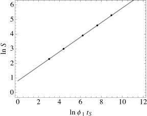
Figure 2: Plume growth in a 1D homogeneous brick. The diagonal line has slope $1/2$, indicating power-law growth with exponent $\gamma=1/2$.

Figure 3: Potential profile $\left\{\phi_{j}\right\}$ for the plume tracked in Fig. 2, at size $S=50$. The profile remains linear as the plume grows.

In this example, and subsequent calculations, the fluid viscosity $\mu=1$.

Note that the value $\mu$ is constant and uniform throughout a plume. In addition, inspection of the WDM equations in Sec. II reveals that all quantities are ultimately functions of ratios $\kappa/\mu$. Thus fluid infiltration of a brick represented by the array of elements $\left\{\frac{\kappa_{j}}{\mu}\right\}$ resembles that for any brick represented by an array having elements $\frac{\kappa^{\prime}_{j}}{\mu^{\prime}}=\frac{\kappa_{j}}{\mu}$. For example, Fig. 2 is reproduced by a 1D brick represented by an array of elements $\frac{\kappa_{j}}{\mu}=\frac{10}{2}$.

V Sierpinski carpets

An interesting 2D brick is the Sierpinski carpet [Sierp, ], which has a self-similar geometric structure comprising a connected domain of permeability $\kappa_{\alpha}$ surrounding disconnected domains of permeability $\kappa_{\beta}$. Figure 4 shows the fifth iteration of the generator for the center-hole $(3,1)$ Sierpinski carpet, which is used in the calculations. There are five sizes of white squares; the smallest white squares are the size of a “site”. Thus the carpet comprises $\left(3^{5}\right)^{2}=243^{2}$ sites. Each brick considered here is a linear array of carpets. The fluid viscosity value $\mu=1$ is used in these calculations.

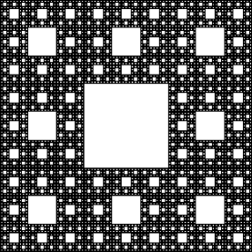
Figure 4: Fifth iteration Sierpinski carpet. The left edge of the carpet is the reservoir/brick interface from which a plume grows. The connected black domain has permeability $\kappa_{\alpha}$ while the distributed white domains have permeability $\kappa_{\beta}$.

The potential field $\left\{\phi\right\}$ is obtained by releasing a very large number of walkers from the reservoir/brick interface (the “source”), and immediately removing them when they move over the plume boundary (the “sink”). For each brick considered below, it is assumed that an accurate representation of the potential field is achieved when $10^{6}$ walkers have reached the sink. Of course, those walkers are accompanied by orders-of-magnitude more walkers that are absorbed at the reservoir/brick interface.

The results for fluid infiltration are presented in log-log plots of $\left\langle\phi_{1}\right\rangle t_{S}$ versus plume size $S$. Points that don’t lie precisely on a fitted line are believed to reflect the details of the carpet geometry, not the stochastic nature of the calculations. To aid comprehension, horizontal lines are added that correspond to a saturated half-carpet (dotted line), and fully saturated carpets (dashed lines) in the array.

Linear array of carpets with $\kappa_{\alpha}=1$ and $\kappa_{\beta}=0$

Figure 5 is the $\log$-$\log$ plot of $\left\langle\phi_{1}\right\rangle t_{S}$ versus plume size $S$. The upper diagonal line is a fit to the points for plumes that are contained within the first carpet. The slope of that line is $\gamma=0.423<1/2$. The progressively smaller $\kappa_{\mathrm{eff}}$ values associated with the advancing (growing) plume can be calculated by Eq. (16). The lower diagonal line has slope $1/2$ and runs through the last point on the plot, obtained for a plume that has entered the fourth carpet in the array. That last point gives the effective permeability $\kappa_{\mathrm{eff}}=0.179$. The lower horizontal dashed line at $S=3^{10}\left(8/9\right)^{5}$ corresponds to a fully saturated single carpet; the upper horizontal dashed line corresponds to a fully saturated two-carpet array.

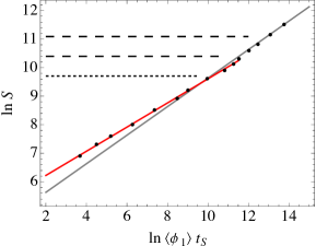
Figure 5: Plume growth into a linear array of Sierpinski carpets with connected domain $\kappa_{\alpha}=1$, and $\kappa_{\beta}=0$. The upper diagonal line is fitted to points for plumes contained within the first carpet, which reveals “anomalous” power-law growth with exponent $\gamma=0.423<1/2$.

Linear array of carpets with $\kappa_{\alpha}=1$ and $\kappa_{\beta}=0.01$

Figure 6 closely resembles Fig. 5, the apparent difference being the somewhat larger exponent value $\gamma=0.463$. The lower diagonal line has slope $1/2$ and runs through the last point on the plot, obtained for a plume that has entered the third carpet in the array. That last point gives the effective permeability $\kappa_{\mathrm{eff}}=0.336$.

Figure 7 is a contour plot of the potential field for a plume of size $S=50000$. The fluid reservoir, kept at constant pressure, is at the left edge of the carpet. Note the steep potential gradient produced in the low-permeability regions. Clearly those regions impede and distort the plume’s advance. However, once a low-permeability domain is saturated, it appears to be less of an impediment to subsequent fluid flow.

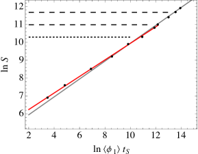
Figure 6: Plume growth into a linear array of Sierpinski carpets with connected domain $\kappa_{\alpha}=1$, and $\kappa_{\beta}=0.01$. The upper diagonal line is fitted to points for plumes contained within the first carpet, which reveals “anomalous” power-law growth with exponent $\gamma=0.463<1/2$.

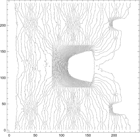
Figure 7: Contour plot of the potential field $\left\{\phi\right\}$ for a plume of size $S=50000$ contained within a carpet with connected domain $\kappa_{\alpha}=1$, and $\kappa_{\beta}=0.01$. This plume contributed a point to Fig. 6.

Linear array of carpets with $\kappa_{\alpha}=1$ and $\kappa_{\beta}=100$

Figure 8 is the log-log plot of $\left\langle\phi_{1}\right\rangle t_{S}$ versus plume size $S$. The lower diagonal line is a fit to the points for plumes that are contained within the first carpet. The slope of that line is $\gamma=0.538>1/2$. The upper diagonal line has slope $1/2$ and runs through the last point on the plot, obtained for a plume that has entered the second carpet in the array. That last point gives the effective permeability $\kappa_{\mathrm{eff}}=2.547$.

Figure 9 is a contour plot of the potential field for a plume of size $S=50000$. The fluid reservoir, kept at constant pressure, is at the left edge of the carpet. Note the very modest potential gradient produced in the high-permeability regions.

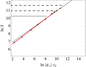
Figure 8: Plume growth into a linear array of Sierpinski carpets with connected domain $\kappa_{\alpha}=1$, and $\kappa_{\beta}=100$. The lower diagonal line is fitted to points for plumes contained within the first carpet, which reveals “anomalous” power-law growth with exponent $\gamma=0.538>1/2$.

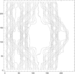
Figure 9: Contour plot of the potential field $\left\{\phi\right\}$ for a plume of size $S=50000$ contained within a carpet with connected domain $\kappa_{\alpha}=1$, and $\kappa_{\beta}=100$. This plume contributed a point to Fig. 8.

Inspection of Figs. 5, 6, and 8 finds that $\xi_{p}$ is not less than one carpet length (measured from the reservoir/brick interface), in each case. In any event the transition implied by $\xi_{p}$ may be rather gradual. That is, the transition to “normal” growth behavior ($\gamma=1/2$) may not be complete until the plume has saturated multiple carpets in the array. Indeed this is true for the examples above: Denote by the function $\kappa\left(\kappa_{\alpha},\kappa_{b}\right)$ the effective permeability $\kappa_{\mathrm{eff}}$ of an infinite, linear array of Sierpinski carpets comprised of domains with permeabilities $\kappa_{\alpha}$ and $\kappa_{\beta}$. Then according to Ref. (Chess, ),

$$\kappa\left(1,0.01\right)\>\kappa\left(1,100\right)=1.$$ (21)

Thus one or both of the calculated $\kappa_{\mathrm{eff}}$ values reported above are too low (their product is $0.856$), so indicating that “normal” growth behavior has not yet been achieved in one or both systems. [Unfortunately, walkers get trapped in the non-percolating $\kappa_{\beta}=100$ domains for long periods of computer time, making calculations for arrays of many carpets infeasible. More points in Fig. 8 would undoubtably reveal the true value $\kappa_{\mathrm{eff}}>2.547$.]

Although a precise numerical value for $\xi_{p}$ is impossible to obtain, it is a useful concept.

Linear array of carpets with connected pore space ($\kappa_{\alpha}=\infty$) and $\kappa_{\beta}=0$

The walker behavior, and so the potential field $\left\{\phi\right\}$, are determined by the domain morphology (geometry) of the brick, and by the ratios of the different permeability values of the domains comprising a brick. Thus application of the fluid infiltration model to the Sierpinski carpet with connected pore space is identical to that for the Sierpinski carpet with permeabilities $\kappa_{\alpha}=1$ and $\kappa_{\beta}=0$. Consequently the “anomalous” exponent value $\gamma=0.423$ is the same in both cases.

This value is identical to that obtained experimentally by Filipovitch et al. [Filip, ] using a Hele-Shaw cell containing a 3D-printed distribution of flow obstacles in the pattern of the second iteration of the generator for the center-hole (3,1) Sierpinski carpet. (This is the pattern of Fig. 4, but with two, rather than five, sizes of white squares.) The fluid was pure glycerin, under a fixed pressure head at one edge of the square carpet. Further, Ref. [Filip, ] and Voller [Voller, ] report simulations (thus an approach different from that used in this paper) that obtain essentially this same value of $\gamma$ for carpets in the pattern of the first, second, third, and fourth iterations. Subsequently, variations on those simulations were made by Aar$\tilde{\mathrm{a}}$o Reis et al. [Aarao, ] to better understand the carpet-plume system.

That the power-law exponent $\gamma$ is the same for carpet iterations $i\leq 5$ is due to the fact that as the plume front moves from the reservoir/brick “source” through the $i=5$ carpet, it is passing through the $i<5$ carpets in turn (see Fig. 4). Thus this is an effect of the self-similar character of the Sierpinski carpet, on the fluid infiltration.

Note that a Sierpinski carpet with connected pore space can be regarded as a homogeneous material with an effective permeability $\kappa_{\mathrm{eff}}$. Clearly that value reflects the porosity $\left(8/9\right)^{i}$ of the carpet. Thus $\kappa_{\mathrm{eff}}$ will decrease as the plume advances through the $i=5$ carpet by filling the $i<5$ carpets in turn. That sequence produces a time-evolution exponent $\gamma<1/2$.

In fact $\kappa_{i}$ will decrease faster than $\left(8/9\right)^{i}$, since the porosity value does not fully account for the distribution of obstacles-to-flow within the carpet. Here $\kappa_{i}$ is the effective permeability for a fully saturated, iteration $i$ Sierpinski carpet. A crude upper bound for the $\gamma$ value is obtained as follows.

Reference [Sierp, ] provides the relation

$$\frac{S_{i}}{W_{i}}=\left(\frac{8}{9}\right)^{i}W_{i}=\left[\left(\frac{8}{9}\right)^{i}\right]^{1-\nu}$$ (22)

where the subscript $i$ refers to the iteration $i$ Sierpinski carpet, and $\nu\equiv\left(2-\mathcal{H}\right)^{-1}$ where $\mathcal{H=\ln}8/\ln 3$ is the Hausdorff (fractal) dimension of the Sierpinski carpet. Then use of Eq. (20) in Eq. (16) gives

$$\frac{\kappa_{i}}{\mu}=\left(\frac{S_{i}}{W_{i}}\right)^{2}\frac{1}{\left\langle\phi_{1}\right\rangle t_{S}}\propto\left(\frac{S_{i}}{W_{i}}\right)^{2}\left(\frac{S_{i}}{W_{i}}\right)^{-1/\gamma}$$ (23)

thereby producing the relation

$$\frac{\kappa_{i}}{\mu}\propto\left[\left(\frac{8}{9}\right)^{i}\right]^{\eta}$$ (24)

with exponent $\eta$ being

$$\eta\equiv\left(1-\nu\right)\left(2-\frac{1}{\gamma}\right).$$ (25)

In order that $\kappa_{i}/\mu$ decrease faster than $\left(8/9\right)^{i}$, the exponent $\eta$ must be greater than $1$. After some algebra, the upper bound is obtained:

$$\gamma<\left(2+\frac{1}{\nu-1}\right)^{-1}=1-\frac{1}{\mathcal{H}}=0.471679$$ (26)

VI Concluding remarks

The stochastic model and method developed here for fluid infiltration of a permeable brick utilizes a local version of Darcy’s law in order to account for the heterogeneities in the brick. For plumes that have not yet advanced a distance $\xi_{p}$ into the brick, the time evolution is “anomalous”, caused by significant variation in the effective permeability $\mathrm{\kappa}_{\mathrm{eff}}$ as the plume grows. Specifically, an exponent $\gamma$ value greater (less) than $1/2$ is produced by growth into regions of generally increasing (decreasing) permeability. Plumes that have advanced beyond $\xi_{p}$ show “normal” behavior, indicated by the exponent value $\gamma=1/2$ (which in fact is a consequence of having little or no variation of $\kappa_{\mathrm{eff}}$ as the plume grows).

Here the method is applied to bricks that are linear arrays of Sierpinski carpets. These are fairly representative bricks, in that they comprise a connected (percolating) domain of permeability $\kappa_{\alpha}$ surrounding isolated domains of permeability $\kappa_{\beta}$. Plume growth within the first carpet presents as a power law with exponent $\gamma\neq 1/2$, in accordance with the plume infiltration model in Sec. IV.

The contour plots of the potential field (illustrating the driving forces for fluid flow within the plume) for carpets with ratio $\kappa_{\beta}/\kappa_{\alpha}$ greater and less than unity show that the flow is much more complicated than simple fast/slow channels. This is because a growing plume is cohesive and incompressible and remains connected to the fluid reservoir. In no respect does it resemble a collection of diffusing particles.

- (1) C. DeW.Van Siclen, Walker diffusion method for calculation of transport properties of composite materials, Phys. Rev. E 59 (3), 2804–7 (1999).
- (2) C. DeW. Van Siclen, Walker diffusion method for calculation of transport properties of finite composite systems, Phys. Rev. E 65, 026144 (2002).
- (3) C. DeW. Van Siclen, Percolation properties of the classic Sierpinski carpet and sponge, e-print arXiv:1706.03410 [Available at https://arxiv.org/abs/1706.03410]
- (4) C. DeW. Van Siclen, Effective conductivity of the multidimensional chessboard, e-print arXiv:2006.16313 [Available at https://arxiv.org/abs/2006.16313]
- (5) N. Filipovitch, K. M. Hill, A. Longjas, and V. R. Voller, Infiltration experiments demonstrate an explicit connection between heterogeneity and anomalous diffusion behavior, Water Resour. Res. 52, 5167–5178 (2016).
- (6) V. R. Voller, A direct simulation demonstrating the role of spacial heterogeneity in determining anomalous diffusive transport, Water Resour. Res. 51, 2119–2127 (2015).
- (7) F. D. A. Aaro Reis, D. Bolster, and V. R. Voller, Anomalous behaviors during infiltration into heterogeneous porous media, Adv. Water Resour. 113, 180–188 (2018).