Statistical properties of the gravitational force in a random homogeneous medium

Abstract

We discuss the statistical distribution of the gravitational (Newtonian) force exerted on a test particle in a infinite random and homogeneous gas of non-correlated particles. The exact solution is known as the Holtsmark distribution at the limit of infinite system corresponding to the number of particle $N$ within the volume and the volume going to infinity. The statistical behaviour of the gravitational force for scale comparable to the inter-distance particle can be analyzed through the combination of the $n$-th nearest neighbor particle contribution to the total gravitational force, which can be derived from the joint probability density of location for a set of $N$ particles. We investigate two independent approaches to derive the joint probability density of location for a set of $N$ neighbors using integral forms and order statistics to give a general expression of such probability distribution with generalised dimension of space. We found that the non-finite dispersion of the Holtsmark distribution is due to the single contribution of the first nearest neighbor in the total gravitational force.

I Introduction

The knowledge of the evolution and the statistical properties of the gravitational field in a infinite self-gravitating system with Poisson-like spatial distribution of masses (stars, galaxies, …) presents an interesting and widely investigated subject of research. The basic mechanism for the emergence of coherent structure in gravitational $N$-body system with long-range interacting sources from an initial spatial and mass distribution, and subject to small fluctuations of density still presents open problems in stellar dynamics, in cosmological $N$-body simulations.

In section II, we review the two-point statistics of a random density field in a homogeneous-universe. We also recall the one-point statistics of a Poisson-like random field, which is the case we are study in this paper. In section III, we recall the derivation of the probability density function of the total gravitational force exerted on an arbitrary particle within a homogeneous isotropic gas of non-correlated particles, known as the Holtsmark distribution. Additional information can be obtained by considering order statistics such as the contribution of a single $n$-th nearest neighbor particle to the total gravitational force exerted on a test particle. In section IV, we recall the properties of the first nearest neighbor spatial probability density function. The nearest neighbor statistical properties is related to the two point auto-correlation function, which has an important status in astrophysics and cosmology. To evaluate each neighbor’s contribution, it requires to get a general expression of the joint probability density function to find the set of $N$ nearest neighbors at respective locations with general dimension of space $d$, from which the corresponding distribution of force can be simply derived. To do so, in section V, we generalize to the $n$-th nearest neighbor spatial probability density function. From the results obtained in section V, we study in section VI the probability density function of the gravitational force exerted by each of the nearest neighbor and derive the dispersion of the total gravitational force in terms of single contributions. We conclude in section VII.

II Density as a stochastic variable

We consider a $d$-volume $v_{d}$ filled with $N$ particles. The local density can be assimilated to a random variable with specific probability distribution. We note the density at location x as the random stochastic variable $\hat{\rho}(\textbf{x})$ given by the number of particle within the elementary volume $\mbox{d}V=\mbox{d}x_{1}\times...\times\mbox{d}x_{d}$. When each particle with index $i$ is at location $\textbf{x}_{i}$, the stochastic density can be expressed by the sum

$$\hat{\rho}(\textbf{x})=\sum\limits_{i=1}^{N}\delta^{(d)}(\textbf{x}-\textbf{x}_{i}),$$ (1)

where $\delta^{(d)}$ is the Dirac delta distribution in dimension $d$. The local average density $\rho(\textbf{x})$ is simply given by the ensemble average $\langle\cdot\rangle$ over all the configurations of particles in the volume $v_{d}$ such as

$$\rho(\textbf{x})=\sum\limits_{i=1}^{N}\langle\delta^{(d)}(\textbf{x}-\textbf{x}_{i})\rangle.$$ (2)

Giving $f(\textbf{x}_{i})$ the probability density function for finding the particle denoted by $i$ within the elementary volume $\mbox{d}V$ around $\textbf{x}_{i}$, the ensemble average is given by

$$\langle\delta^{(d)}(\textbf{x}-\textbf{x}_{i})\rangle=\int_{v_{d}}\mbox{d}^{d}\textbf{x}_{i}f(\textbf{x}_{i})\delta^{(d)}(\textbf{x}-\textbf{x}_{i}).$$ (3)

When particles are non-correlated, the probability for occupying the volume $\mbox{d}V$ does not depend on position. Then $f(\textbf{x}_{i})$ is a constant over space, and the ensemble average of the Dirac distribution results in $\langle\delta^{(d)}(\textbf{x}-\textbf{x}_{i})\rangle=1/v_{d}$. The local average density is deduced by the sum over the $N$ indexes $i$ giving $\rho_{0}(\textbf{x})=\rho_{0}=N/v_{d}$.

II.1 Auto-correlation function

we define the reduced correlation function $\xi$ as the ensemble average (Sylos Labini & Pietronero 2008)

$$\xi(r)=\langle\delta(\textbf{x}_{1})\delta(\textbf{x}_{2})\rangle,$$ (4)

where $r=|\textbf{x}_{1}-\textbf{x}_{2}|$ and $\delta(\textbf{x})=(\hat{\rho}(\textbf{x})-\rho_{0})/\rho_{0}$ is the reduced density perturbation over space. the radial dependence $\xi(\textbf{x})=\xi(r)$ is due to the assumption of homogeneous isotropic gas of particles. By using the definition of the local density in Eq. (1) and the joint probability density in Eq. (21), the ensemble average $\langle\hat{\rho}(\textbf{x}_{1})\hat{\rho}(\textbf{x}_{2})\rangle$ can be expressed after development

$$\langle\hat{\rho}(\textbf{x}_{1})\hat{\rho}(\textbf{x}_{2})\rangle =\sum\limits_{i,j=1}^{N}\langle\delta^{(d)}(\textbf{x}_{1}-\textbf{x}_{i})\delta^{(d)}(\textbf{x}_{2}-\textbf{x}_{j})\rangle$$ (5)

$$=\sum\limits_{i=1}^{N}f_{i,i}(\textbf{x}_{1},\textbf{x}_{2})+\sum\limits_{i\neq j=1}^{N}f_{i,j}(\textbf{x}_{1},\textbf{x}_{2}),$$ (6)

where $f_{i,j}(\textbf{x}_{1},\textbf{x}_{2})$ is the joint probability density function to find respectively the $i-$th and the $j-$th particle at location $\textbf{x}_{1}$ and $\textbf{x}_{2}$. In the case of a random homogeneous media, the marginal density $f_{i}(\textbf{x})=1/v_{d}$. Then, without loss of generality we can write

$$f_{i,j}(\textbf{x}_{1},\textbf{x}_{2})=\frac{1}{v_{d}}w_{i,j}(\textbf{x}_{1}|\textbf{x}_{2}),$$ (7)

where $w_{i,j}(\textbf{x}_{1}|\textbf{x}_{2})$ is the conditional probability to find the $i-$th particle at location $\textbf{x}_{1}$ knowing that the $j-$th particle is at location $\textbf{x}_{2}$. For homogeneous and isotropic gas, probability density function $f_{i,j}$ does not depend on indexes $i$ and $j$ when $i\neq j$, then we have

$$w_{i,j}(\textbf{x}_{1}|\textbf{x}_{2})=\left\{\begin{array}[]{ll}\delta^{(d)}(|\textbf{x}_{1}-\textbf{x}_{2}|)&\mbox{if }\ i=j\\ w(|\textbf{x}_{1}-\textbf{x}_{2}|)&\mbox{if }\ i\neq j\end{array}\right.$$ (8)

Then we can derive

$$\langle\rho(\textbf{x}_{1})\rho(\textbf{x}_{2})\rangle =\rho_{0}\delta^{(d)}(r)+\frac{N(N-1)}{v_{d}}w(r)$$ (9)

$$\approx\rho_{0}\delta^{(d)}(r)+N\rho_{0}w(r).$$ (10)

The function $w$ is the probability density to find a given particle within an elementary volume at a distance $r$ and verifies the normalization

$$\int_{v_{d}}\mbox{d}^{d}\textbf{x}w(|\textbf{x}|)=1.$$ (11)

The correlation function $\xi(r)$ expresses as

$$\xi(r)=\frac{\delta^{(d)}(r)}{\rho_{0}}+\frac{N}{\rho_{0}}w(r)-1.$$ (12)

Then, the $w$ function reaches the expression in term of $\xi$ giving

$$w(r)=\frac{1}{v_{d}}[1+\xi(r)].$$ (13)

The function $\xi$ appears as a probability excess. It characterises a deviation to the probability density function $1/v_{d}$ and following this convention, we have three possible cases,

$$\xi(r):\left\{\begin{array}[]{ll}>0&\mbox{particles tend to attract each other}\\ =0&\mbox{particles are uncorrelated}\\ <0&\mbox{particles tend to repel each other}\end{array}\right.$$ (14)

and the $\xi$ function verifies the integration

$$\frac{1}{v_{d}}\int_{v_{d}}\xi(r)\mbox{d}^{d}\textbf{x}=0.$$ (15)

We now get the probability $w(r)$ to find a given particle at distance $r$ knowing a particle is at location $r=0$. The probability density function $G$ to find a particle at location $r$ regardless is index $i$ is the sum over all the particles in the gas of $w_{i}$ (excepted for the center particle), such that

$$G(r)=\sum\limits_{i=1}^{N-1}w_{i}(r)\approx\rho_{0}[1+\xi(r)]$$ (16)

II.2 The Poisson point process

The probability $q$ for a given particle for being in a elementary volume $\mbox{d}V$ within the total volume $v_{d}$ is $q=\mbox{d}V/v_{d}$. We consider the random variable $\mathcal{N}$ as the number of particles within the elementary volume $\mbox{d}V$. When particles are non-correlated (independent), $\mathcal{N}$ follows a binomial law with parameter $q$ given by

$$\mathbb{P}(\mathcal{N}=n)=\frac{N!}{n!(N-n)!}q^{n}(1-q)^{N-n}.$$ (17)

The Poisson limit Theorem is valid when the total number of particles $N\gg n$ and the probability $q\ll 1$. We consider the number of particle $N$ and the volume $v_{d}$ going to infinity, as the density $\rho_{0}$ keeps constant. Noting the average of the binomial law as $\lambda=Nq=\rho_{0}\mbox{d}V$, and verifying $\lambda\ll 1$, the Poisson limit theorem gives the distribution

$$\lim_{N,v_{d}\to\infty}\mathbb{P}(\mathcal{N}=n)=\frac{\lambda^{n}}{n!}\exp[-\lambda]\approx\frac{\lambda^{n}}{n!}(1-\lambda),$$ (18)

with $\mathbb{P}(0)$ and $\mathbb{P}(1)$ much higher than $\mathbb{P}(n>1)$ which is proportional to $(\rho_{0}\mbox{d}V)^{n}$. The stochastic local density $\hat{\rho}(\textbf{x})$ verifies the probability distribution

$\hat{\rho}(\textbf{x})=\left\{\begin{array}[]{rl}\frac{1}{\mbox{d}V}&\mbox{with probability}\ \rho_{0}\mbox{d}V\\ 0&\mbox{with probability}\ 1-\rho_{0}\mbox{d}V\end{array}\right.$

Either the volume is occupied by a particle with probability $\rho_{0}\mbox{d}V$ or it is empty with the complementary probability $1-\rho_{0}\mbox{d}V$. The average gives the density $\langle\hat{\rho}(\textbf{x})\rangle=\rho_{0}$.

III The Holtsmark distribution

In dimension $d=3$, we note $v_{3}=V$. We consider a test particle of mass $m$ located at x in a gas of identical particles of mass $m$ denoted by $i$. The total gravitational force F exerted on the test particle by its neighborhood can be obtained by the vectorial sum over all the particle contributions at respective location $\textbf{x}_{i}$ and is given by

$$\textbf{F}(\textbf{x})=\sum\limits_{i=1}^{N}\frac{Gm^{2}}{|\textbf{x}_{i}-\textbf{x}|^{3}}(\textbf{x}_{i}-\textbf{x})=\sum\limits_{i=1}^{N}\textbf{F}_{i},$$ (19)

with the gravitational constant $G=6,674\times 10^{-11}\ \mbox{m}^{3}.\mbox{kg}^{-1}.\mbox{s}^{-2}$. We can give a general expression to the probability density function $W(\textbf{F})$ to find the gravitational force exerted on the test particle comprised in a small volume $\mbox{d}^{3}\textbf{F}$ around F due to all the $N$ particles in a sphere centered on it. Such probability can be expressed as (Pietronero et al. 2002)

$$W(\textbf{F})=\int_{V}...\int_{V}\mbox{d}\textbf{x}^{3N}f(\textbf{x}_{1},...,\textbf{x}_{N})\delta\left(\textbf{F}-\sum\limits_{i}^{N}\textbf{F}_{i}\right),$$ (20)

where $f(\textbf{x}_{1},...,\textbf{x}_{N})$ is the joint probability density function to find the $N$ particles at location $\textbf{x}_{1},...,\textbf{x}_{N}$.

We present the steps to reach the expression of the probability density function of force F for non-correlated particles with equal mass $m$. In this case, the joint probability function $f$ is the product of the constant probability density function for each particle given by $1/V$. The probability that the $n$ particle occupies the volume $d\textbf{x}^{3N}$ is given by

$$f(\textbf{x}_{1},...,\textbf{x}_{N})\mbox{d}\textbf{x}^{3N}=\frac{\mbox{d}\textbf{x}^{3N}}{V^{N}}.$$ (21)

The distribution of force is then given by the integral over $N$ volumes

$$W_{H}(\textbf{F})=\int_{V}...\int_{V}\left[\frac{\mbox{d}\textbf{x}^{3N}}{V^{N}}\right]\delta\left(\textbf{F}-\sum\limits_{i}^{N}\textbf{F}_{i}\right).$$ (22)

By giving the expression of $W_{H}$ as a inverse Fourier transform, we get

$$W_{H}(\textbf{F})=\frac{1}{(2\pi)^{3}}\int_{\Omega(\textbf{k})}\mbox{d}^{3}\textbf{k}A(\textbf{k})\exp(-i\textbf{k}\cdot\textbf{F}),$$ (23)

where $A(\textbf{k})$ is given by

$$A(\textbf{k}) =\left[\int_{V}\frac{\mbox{d}^{3}\textbf{x}}{V}\exp(i\textbf{k}\cdot\textbf{F}_{i}(\textbf{x}))\right]^{N}$$ (24)

$$=\left[1-\frac{\rho_{0}}{\rho_{0}V}\int_{V}\mbox{d}^{3}\textbf{x}[1-\exp(i\textbf{k}\cdot\textbf{F}_{i}(\textbf{x}))]\right]^{\rho_{0}V}.$$ (25)

By using the definition of the exponential function, for infinite volume $v_{d}$, infinite number of particle $N$, and constant density $\rho_{0}$, we get

$$A(\textbf{k})=\lim_{N\to\infty}\left[1-\frac{\rho_{0}C(\textbf{k})}{N}\right]^{N}=\exp(-\rho_{0}C(\textbf{k})),$$ (26)

with

$$C(\textbf{k})=\int_{V}\mbox{d}^{3}\textbf{x}[1-\exp(i\textbf{k}\cdot\textbf{F}_{i}(\textbf{x}))].$$ (27)

By considering an arbitrary axis given by the vector k, integrating over all the directions gives

$$C(k) =2\pi(kGm^{2})^{3/2}\int_{0}^{\infty}\frac{\mbox{d}u}{u^{5/2}}\left[u-\sin(u)\right]$$ (28)

$$=\frac{4}{15}(2\pi kGm^{2})^{3/2}.$$ (29)

where we used Eq. (151) to identify

$$\int_{0}^{\infty}\frac{\mbox{d}u}{u^{5/2}}\left[u-\sin(u)\right]=\int_{0}^{\infty}\frac{\sin(u)}{u^{3/2}}\mbox{d}u=\frac{4\sqrt{2\pi}}{15}.$$ (30)

The Holtsmark distribution is given by the integral

$$W_{H}(\textbf{F})=\frac{1}{(2\pi)^{3}}\int_{\Omega(\textbf{k})}\mbox{d}^{3}\textbf{k}\exp[-i\textbf{k}\cdot\textbf{F}-\frac{4\rho_{0}}{15}(2\pi kGm^{2})^{3/2}].$$ (31)

By considering, as before, an arbitrary axis oriented along F giving $\textbf{k}\cdot\textbf{F}=kF\cos{\theta}$, integrating over the directions and radial variable $k$ gives the expression

$$W_{H}(\textbf{F})=\frac{1}{2\pi^{2}F^{3}}\int_{0}^{\infty}\mbox{d}x(x\sin{x})\exp\left[-(x/\beta)^{3/2}\right]$$ (32)

where $\beta=F/F_{0}$ and the typical force $F_{0}$ defined as

$$F_{0}=2\pi\left(\frac{4}{15}\right)^{2/3}\frac{Gm^{2}}{\lambda^{2}},$$ (33)

with $\lambda=\rho_{0}^{-1/3}$ the length measure associated to the average inter-particle separation. The Holtsmark distribution (e.g. Chandrasekhar (1943), Sylos Labini & Pietronero (2008), Chavanis (2009)) for the modulus $F=|\textbf{F}|$ (represented in Figure 2) is given by integrating overall the directions

$$W_{H}(F)=\frac{2}{\pi F}\int_{0}^{\infty}\mbox{d}x(x\sin{x})\exp[-(x/\beta)^{3/2}].$$ (34)

The average force is given by the integral

$$\langle F\rangle=F_{0}^{2}\int_{0}^{\infty}\beta W_{H}(\beta)\mbox{d}\beta=\frac{4F_{0}}{\pi}\Gamma\left(\frac{1}{3}\right)\approx 3.412F_{0}.$$ (35)

The dispersion of the Holtsmark distribution is not finished. We can investigate two specific regimes; for $F\rightarrow 0$, it is required to develop $W$ in series by using the the Taylor expansion of $\sin(x)$ in Eq. (149) giving

$$W_{H}(F)=\frac{2}{\pi\beta F_{0}}\sum\limits_{n=0}\frac{(-1)^{n}}{(2n+1)!}\int^{\infty}_{0}x^{2n+1}\exp[-(x/\beta)^{3/2}]\mbox{d}x.$$ (36)

Recognizing the Gamma-Euler function in Eq. (146), the sum becomes

$$W_{H}(F)=\frac{4}{3\pi F_{0}}\sum\limits_{n=0}\frac{(-1)^{n}}{(2n+1)!}\Gamma\left(\frac{2n+3}{3/2}\right)\beta^{2n+2}.$$ (37)

The first two term of the sum are reported in the case of the regime $\beta\rightarrow 0$, giving

$$W_{H}(F)\approx\frac{4}{3\pi F_{0}}\beta^{2}-\frac{2}{9\pi F_{0}}\Gamma\left(\frac{10}{3}\right)\beta^{4}.$$ (38)

For $\beta\rightarrow\infty$, we now use the Taylor expansion of the exponential function in Eq. (150) giving

$$W_{H}(F)=\frac{2}{\pi F_{0}}\sum\limits_{n=0}\frac{(-1)^{n}}{n!}\beta^{-(3n/2+1)}\int_{0}^{\infty}x^{3n/2+1}\sin x\mbox{d}x,$$ (39)

giving the explicit formula for $W_{H}(F)$ using Eq. (151)

$$W_{H}(F) =\frac{2}{\pi F_{0}}\sum\limits_{n=0}\frac{(-1)^{n+1}}{n!}\sin\left(\frac{3\pi n}{4}\right)\times$$ (40)

$$\Gamma\left(\frac{3n}{2}+2\right)\beta^{-(3n/2+1)}.$$ (41)

Reporting the two first non-zero terms for large $F$, we get

$$W_{H}(F)\approx\frac{15}{8F_{0}}\left(\frac{2}{\pi}\right)^{1/2}\beta^{-5/2}-\frac{24}{\pi F_{0}}\beta^{-4}.$$ (42)

IV First nearest neighbor density function

We investigate the statistical properties of the first nearest neighbor of a random particle in a gas with Poisson-like distribution of particles in general dimension $d$. We first consider a homogeneous and isotropic gas of particle, and then we treat the Poisson-like case. The probability density function $w_{1}(r)$ to find the nearest neighbor particle at a distance comprises between $r$ and $r+dr$ from an arbitrary particle is given by the ensemble average (Chandrasekhar (1943), Mazur (1992))

$$w_{1}(r)=\left\langle\sum\limits_{j=2}^{N}\delta(r-r_{j})\prod\limits^{N}_{k\neq(i,j)}\left[1-\int_{0}^{r}\delta(x-r_{k})\mbox{d}x\right]\right\rangle,$$ (43)

where $r_{j}$ is the distance of the $j$-th particle around the center particle. The nearest neighbor density function takes the form

$$w_{1}(r)=\left[1-\int_{0}^{r}w_{1}(u)\mbox{d}u\right]G(r)\alpha_{d}r^{d-1}.$$ (44)

The general solution of function defined such that

$$g(x)=f(x)\int_{x}^{\infty}g(u)\mbox{d}u,$$ (45)

with $K$ an appropriated constant. We then get

$$g(x)=Kf(x)\exp\left(-\int_{0}^{x}f(u)\mbox{d}u\right).$$ (46)

We define $N(r)=\rho_{0}\alpha_{d}r^{d}/d=(r/\lambda_{d})^{d}$ the average number of particles within the $d$-volume or radius $r$ with the typical measure of length $\lambda_{d}$ given by

$$\lambda_{d}=\left[\frac{d}{\rho_{0}\alpha_{d}}\right]^{1/d}.$$ (47)

We can write the density $w_{1}(r)$ after normalization

$$w_{1}(r)=N^{\prime}(r)(1+\xi(r))\mbox{e}^{-N(r)+\int_{0}^{r}N^{\prime}(x)\xi(x)\mbox{d}x}.$$ (48)

The assumption of a Poisson distribution of particle means particles are uncorrelated, such that the auto-correlation function gets $\xi(r)=0$ if $r\neq 0$. We can write the density $w_{1}(r)$ as

$$w_{1}(r)=N^{\prime}(r)\exp[-N(r)]=(1-\exp[-N(r)])^{\prime}.$$ (49)

In dimension $d=3$, we get naturally

$$w_{1}(r)=4\pi\rho_{0}r^{2}\exp\left[-\frac{4\pi\rho_{0}r^{3}}{3}\right].$$ (50)

Giving the average distance $\langle r\rangle_{1,d}$ of the nearest neighbor particle as the integral

$$\langle r\rangle_{1,d} =\int_{0}^{\infty}w_{1}(r)r\mbox{d}r=\lambda_{d}\Gamma\left(\frac{d+1}{d}\right)$$ (51)

$$\approx 0.554\rho_{0}^{-1/3}\ (\mbox{for $d=3$}),$$ (52)

and the average square distance $\langle r^{2}\rangle_{1,d}$

$$\langle r^{2}\rangle_{1,d} =[\lambda_{d}]^{2}\Gamma\left(\frac{d+2}{d}\right)$$ (53)

$$\approx 0.347\rho_{0}^{-2/3}\ (\mbox{for $d=3$}).$$ (54)

The dispersion $\sigma_{1,d}$ is obtained by combining previous results, such as

$$\sigma_{1,d} =\lambda_{d}\left[\Gamma\left(\frac{d+2}{2}\right)-\Gamma^{2}\left(\frac{d+1}{d}\right)\right]^{1/2}$$ (55)

$$\approx 0.202\rho_{0}^{-1/3}\ (\mbox{for $d=3$}).$$ (56)

As an example, We detail in appendix A the derivation of the mean inter-distance particle when considering non-zero auto-correlation function, describing the statistical properties of un-correlated particles but with finite size with given radius $a$.

V The $n>1$ nearest neighbor particles

We now consider a set of $N$ particles denoted by respective distance $r_{i}$ from a particle at $r=0$. The joint probability density function of finding the $N$ neighbors at distance $r_{1},...,r_{N}$ must fulfill the condition

$$w(r_{1},...,r_{N})=\prod_{i>j}^{N}\Theta(r_{i}-r_{j})w(r_{1},...,r_{N}),$$ (57)

where the normalization can be written as

$$1=\int_{0}^{\infty}\mbox{d}r_{1}...\int_{r_{N-2}}^{\infty}\mbox{d}r_{N-1}\int_{r_{N-1}}^{\infty}\mbox{d}r_{N}w(r_{1},...,r_{N}).$$ (58)

We give the final result before developing the mathematical aspects

$$w(r_{1},...,r_{N})=\prod_{i=N}^{1}N^{\prime}(r_{i})\mbox{e}^{-N(r_{N})}.$$ (59)

First, we try to determine the joint probability density function $w(r_{1},r_{2})$ for finding the first neighbor at a distance $r_{1}$ and the second nearest neighbor at $r_{2}$. It is necessary that the density verifies $w(r_{1},r_{2})=0\ \mbox{if}\ r_{1}>r_{2}$. The joint probability density function $w(r_{1},r_{2})$ can be written in general terms using conditional probability (using the Bayes theorem)

$$w(r_{1},r_{2}) =w_{1}(r_{1})g_{2}(r_{2}|r_{1})$$ (60)

$$=w_{2}(r_{2})g_{1}(r_{1}|r_{2}),$$ (61)

where the $g(a|b)$ are the conditional probability density function of the occurrence of event $a$ assuming event $b$ to occur. We can write an equivalent expression, for the conditional probability $g_{2}(r_{2}|r_{1})$ to find the second nearest neighbor at $r_{2}$ assuming the first nearest neighbor is at $r_{1}$, verifying the integral equation of the same form as in Eq. (45) giving

$$g_{2}(r_{2}|r_{1})=\varphi(r_{1},r_{2})\int_{r_{2}}^{\infty}g(x|r_{1})\mbox{d}x,$$ (62)

verifying the general solution given by (46)

$$g_{2}(r_{2}|r_{1})=\mu(r_{1})\varphi(r_{1},r_{2})\mbox{e}^{-\int_{r_{1}}^{r_{2}}\varphi(r_{1},x)\mbox{d}x}.$$ (63)

Here, $\mu$ is a function of the variable $r_{1}$. The normalization for the conditional probability imposes that

$$1 =\int_{r_{1}}^{\infty}g_{2}(y|r_{1})\mbox{d}y=-\mu(r_{1})\left[\mbox{e}^{-\int_{r_{1}}^{y}\varphi(r_{1},x)\mbox{d}x}\right]^{\infty}_{r1}$$ (64)

$$=\mu(r_{1})(1-\exp[-I(r_{1})]),$$ (65)

where $I(r_{1})$ is the integral

$$I(r_{1})=\int_{r_{1}}^{\infty}\varphi(r_{1},x)\mbox{d}x$$ (66)

We can rewrite the joint probability density function $w(r_{1},r_{2})$ in terms of the function $\varphi$

$$w(r_{1},r_{2})=\frac{w_{1}(r_{1})}{1-\exp[-I(r_{1})]}\varphi(r_{1},r_{2})\mbox{e}^{-\int_{r_{1}}^{r_{2}}\varphi(r_{1},x)\mbox{d}x}.$$ (67)

We note that $\varphi$ has the dimension of a density for a single variable ($\sim L^{-1}$). We can express the $\varphi$ function in terms of the dimensionless quantity $\phi(r_{1},r_{2})>0$ by using the probability $N^{\prime}(r_{2})$ to find a particle at $r_{2}$ regardless its index

$$\varphi(r_{1},r_{2})=N^{\prime}(r_{2})\phi(r_{1},r_{2}).$$ (68)

This expression leads to the following system; knowing that $f$ verifies $f(0)=0$ and admits first derivative it is possible to find another function $\nu$ verifying

$$f(y) =\int_{0}^{y}f^{\prime}(x)\mbox{d}x,$$ (69)

$$=\int_{0}^{y}\nu(x,y)\mbox{d}x.$$ (70)

We note that this situation happens when we express the marginal density $w_{2}$ in the two different ways

$$w_{2}(r_{2}) =\int_{0}^{r_{2}}w_{2}^{\prime}(x)\mbox{d}x,$$ (71)

$$=\int_{0}^{r_{2}}w(x,r_{2})\mbox{d}x.$$ (72)

Now, we assume that the $\phi$ function only depends on the location of the first nearest neighbor $r_{1}$. $I(r_{1})$ diverges to $\infty$ and we get the general form of the joint density $w(r_{1},r_{2})$ in terms of $\phi(r_{1})$

$$w(r_{1},r_{2})=w_{1}(r_{1})N^{\prime}(r_{2})\phi(r_{1})\mbox{e}^{-\phi(r_{1})[N(r_{2})-N(r_{1})]}.$$ (73)

It is crucial to note that the marginal density $w_{1}$ for the first nearest neighbor doesn’t depend on the specific form of the $\phi$ function, because the normalization implies in Eq. (60) such as

$$w_{1}(r_{1})=w_{1}(r_{1})\int_{r_{1}}^{\infty}g_{2}(x|r_{1})\mbox{d}x.$$ (74)

However, the $w_{2}$ density reaches the integral form, with a suitable change of variable ($r\ \rightarrow\ N(r)$)

$$w_{2}(r_{2})=N^{\prime}(r_{2})\int_{0}^{N(r_{2})}\mbox{e}^{-\phi(x)[N(r_{2})-x]-x}\phi(x)\mbox{d}x.$$ (75)

We can investigate the case $\phi(x)=1$, which doesn’t precise particular condition for the first nearest neighbor to be full-filled in the expression of the conditional probability $g_{2}(r_{2}|r_{1})$ in Eq. (62). We get the marginal density $w_{2}(r_{2})$ given by, with appropriated normalization

$$w_{2}(r_{2})=N^{\prime}(r_{2})N(r_{2})\mbox{e}^{-N(r_{2})},$$ (76)

leading to the joint density $w(r_{1},r_{2})$ given by

$$w(r_{1},r_{2})=w_{1}(r_{1})w_{1}(r_{2})\exp[N(r_{1})].$$ (77)

We can now discussed the case for a set of $N$ particles. In general, a joint probability density function takes the form

$$w(r_{1},...,r_{N})=w_{1}(r_{1})\prod_{i=2}^{N}w(r_{i}|r_{i-1},...,r_{1}),$$ (78)

where the term $w(r_{i}|r_{i-1},...,r_{1})$ means the probability density function of finding the $i$-th nearest neighbor at a distance $r_{i}$ assuming the respective locations of the $n=1,...i-1$ nearest neighbors. It verifies $w(r_{i}|r_{i-1},...,r_{1})=0$ if $r_{i}<r_{i-1},...,r_{1}$. We can use the same property $\phi=1$ for the conditional probabilities as expressed in Eq. (62) which was valid for two nearest neighbors. We can write the conditional probability $w(r_{i}|r_{i-1},...,r_{1})$ as follow

$$w(r_{i}|r_{i-1},...,r_{1})=N^{\prime}(r_{i})\int_{r_{i}}^{\infty}w(x|r_{i-1},...,r_{1})\mbox{d}x,$$ (79)

which verifies the solution

$$w(r_{i}|r_{i-1},...,r_{1})=N^{\prime}(r_{i})\exp[-N(r_{i})+N(r_{i-1})].$$ (80)

Then, the joint probability can be written as

$${2}w(r_{1},...,r_{N}) =w_{1}(r_{1})\prod_{i=2}^{N}N^{\prime}(r_{i})\mbox{e}^{\sum\limits_{i=2}^{N}-N(r_{i})+N(r_{i-1})}$$ (81)

$$=\prod_{i=N}^{1}N^{\prime}(r_{i})\mbox{e}^{-N(r_{N})}.$$ (82)

with Heaviside explicit development, we get the general form

$$w(r_{1},...,r_{N})=w_{1}(r_{N})\prod_{i=1}^{N-1}\left[N^{\prime}(r_{i})\prod_{j=1}^{i-1}\Theta(r_{i}-r_{j})\right].$$ (83)

V.1 Marginal density of location for the $n$-th nearest neighbor

For a given index $n\leq N$, we evaluate the density $w(r_{1},...,r_{n})$ by integrating the joint density over the configurations of the particles with index from $n+1$ to $N$

$$w(r_{1},...,r_{n}) =\prod_{i=1}^{n}N^{\prime}(r_{i})\int_{r_{n}}^{\infty}\mbox{d}r_{n+1}...\int_{r_{N-1}}^{\infty}\mbox{d}r_{N}\times$$ (84)

$$\prod_{j=n+1}^{N}N^{\prime}(r_{j})\mbox{e}^{-N(r_{N})}$$ (85)

$$=\prod_{i=1}^{n}N^{\prime}(r_{i})\exp[-N(r_{n})].$$ (86)

The marginal density of index $n$ noted $w_{n}(r)$ (represented in Figure 2) is simply given by integrating $w(r_{1},...,r_{n})$ over the configurations of the particles with index from $1$ to $n-1$

$$w_{n}(r) =N^{\prime}(r)\mbox{e}^{-N(r)}\int_{0}^{r}\mbox{d}r_{n-1}...\int_{0}^{r_{2}}\mbox{d}r_{1}\prod_{i=1}^{n-1}N^{\prime}(r_{i})$$ (87)

$$=\frac{1}{(n-1)!}N^{\prime}(r)N(r)^{n-1}\mbox{e}^{-N(r)},$$ (88)

using the Cauchy formula for repeated integration

$$I_{n}(x) =\int_{a}^{x}dx_{n-1}\int_{a}^{x_{n-1}}dx_{n-2}...\int_{a}^{x_{2}}dx_{1}f(x_{1})$$ (89)

$$=\frac{1}{(n-2)!}\int_{a}^{x}(y-x)^{n-2}f(y)dy.$$ (90)

We can verify that the probability to find a particle at $r$ regardless its index $n$ given by $G(r)$ corresponds to the function $N^{\prime}(r)$ by the sum

$$G(r)=\sum\limits_{n=1}^{\infty}w_{n}(r)=N^{\prime}(r)\mbox{e}^{-N(r)}\sum\limits_{n=0}^{\infty}\frac{N(r)^{n}}{n!}=N^{\prime}(r),$$ (91)

we found consistent result with Eq. (16). We discuss in appendix B an alternative derivation of the $n$-th nearest neighbor probability density function $w_{n}$ using order statistics. The cumulative probability distribution is given by

$$\Omega_{n}(r)=\int_{0}^{r}w_{n}(x)\mbox{d}x=\frac{\gamma(n,N(r))}{(n-1)!}.$$ (92)

The moment of order $k$ $\langle r^{k}\rangle_{n,d}$ is given by the integral

$$\langle r^{k}\rangle_{n,d}=\int_{0}^{\infty}x^{k}w_{n}(x)\mbox{d}x=\frac{[\lambda_{d}]^{k}}{(n-1)!}\Gamma\left(\frac{k}{d}+n\right),$$ (93)

with the limit for large $n$ of the Gamma-Euler function, given by using the Stirling approximation

$$\lim_{n\to\infty}\frac{\Gamma(n+\alpha)}{\Gamma(n)n^{\alpha}}=1.$$ (94)

Using Eq. (94), we get $\langle r^{k}\rangle_{n,d}\approx[\lambda_{d}]^{k}n^{k/d}$ for large $n$, which is the main field approximation for the the asymptotic behaviour considering the mean radius being the radius of a $d$-sphere containing the average number of particle $n=\rho_{0}\alpha_{d}r^{d}/d$, such that

$$\langle r\rangle_{n,d}\approx\left[\frac{dn}{\rho_{0}\alpha_{d}}\right]^{1/d}\propto\langle r\rangle_{1,d}n^{1/d}.$$ (95)

We can evaluate the dispersion $\sigma_{n,d}$

$$\sigma_{n,d}=\frac{\lambda_{d}}{\sqrt{(n-1)!}}\left[\Gamma\left(\frac{2}{d}+n\right)-\frac{\Gamma^{2}(1/d+n)}{(n-1)!}\right]^{1/2}.$$ (96)

We note that for dimension $d=1$ we get the dispersion $\sigma_{n,1}=\lambda_{d}\sqrt{n}$. The dispersion diverges when $n$ increases contrary for dimensions $d>1$ (Figure 1). As the relative error $\sigma_{n,d}/\langle r\rangle_{n,d}$ converges to 0 when $n$ increases (Figure 1).

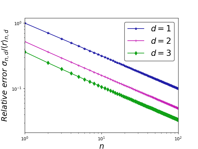
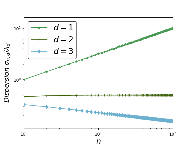
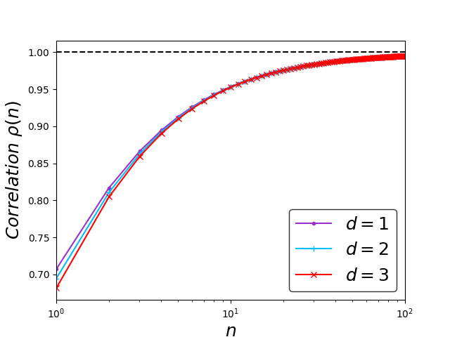
Figure 1: Left - Relative error $\sigma_{n,d}/\langle r\rangle_{n,d}$. Middle - dispersion $\sigma_{n,d}/\lambda_{d}$ as a function of the index $n$. Right - Correlation coefficient $\rho(n)$ of the random variable $r_{n}$ and $r_{n+1}$ in several dimensions of space.

V.2 Joint density of location for two successive nearest neighbors

The joint probability to find two successive nearest neighbors with index $n$ and $n+1$ at respective distances $r_{n}$ and $r_{n+1}$ can be evaluated by the $n-1$ integral of $w(r_{1},...,r_{n+1})$

$$w(r_{n},r_{n+1}) =\int_{0}^{r_{n}}\mbox{d}r_{n-1}...\int_{0}^{r_{2}}\mbox{d}r_{1}w(r_{1},...,r_{n+1})$$ (97)

$$=\frac{N(r_{n})^{n-1}}{(n-1)!}N^{\prime}(r_{n})N^{\prime}(r_{n+1})\mbox{e}^{-N(r_{n+1})}.$$ (98)

The correlation coefficient $\rho(n)$ for the two random variables $r_{n}$ and $r_{n+1}$ follows the expression

$$\rho(n)=\frac{\langle r_{n}r_{n+1}\rangle-\langle r_{n}\rangle\langle r_{n+1}\rangle}{\sigma_{n,d}\sigma_{n+1,d}}.$$ (99)

It requires to calculate the average $\langle r_{n}r_{n+1}\rangle$ by using the conditional probability $g(r_{n}|r_{n+1})$ to find the $n$-th nearest neighbor at $r_{n}$ assuming the $n+1$-th nearest neighbor is at $r_{n+1}$

$$\langle r_{n}r_{n+1}\rangle=\int_{0}^{\infty}\mbox{d}xw_{n+1}(x)x\int_{0}^{r_{n+1}}\mbox{d}yg_{n}(y|x)y,$$ (100)

with the conditional probability $g(r_{n}|r_{n+1})$ given by the ratio

$$g(r_{n}|r_{n+1}) =\frac{w(r_{n},r_{n+1})}{w_{n+1}(r_{n+1})}$$ (101)

$$=n\frac{N(r_{n})^{n-1}}{N(r_{n+1})^{n}}N^{\prime}(r_{n}).$$ (102)

The average $\langle r_{n}r_{n+1}\rangle$ becomes

$$\langle r_{n}r_{n+1}\rangle=\frac{\lambda_{d}^{2}}{(n-1)!}\frac{1}{n+1/d}\Gamma\left(n+1+\frac{2}{d}\right),$$ (103)

where we can generalize to $\langle r_{i}r_{j}\rangle$ with $i<j$

$$\langle r_{i}r_{j}\rangle=\frac{\lambda_{d}^{2}}{(i-1)!}\left(\prod\limits_{k=1}^{j-i}\left[\frac{1}{d}+j-k\right]\right)^{-1}\Gamma\left(\frac{2}{d}+j\right).$$ (104)

We plot the correlation coefficient $\rho$ as a function of the index $n$ of the first particle within the pair $(n,n+1)$ in Figure 1. We first note that correlation is not strongly affected by the dimension $d$ of the space. Besides, the radial coordinates $r_{n}$ and $r_{n+1}$ are strongly correlated when the index of the pair $n$ increases. It describes the increasing accumulation of particles within the layers of arbitrary thickness at distance $R_{n}\propto n^{1/d}\lambda_{d}$ surrounding the $d$-sphere centered of the test particle, due to geometrical effects. Let’s note that the correlation between the vectorial positions $\textbf{x}_{n}$ and $\textbf{x}_{n+1}$ necessary decreases with $n$ in dimension $d>1$. In this section, we discussed the general expression of the density $w_{n}$ for finding any nearest neighbor with index $n$ at location $r$. Such distribution can be used to evaluate the respective contribution of each $n$-th nearest neighbor to the gravitational force exerted on the center particle at $r=0$ due to its neighborhood.

VI Nearest neighbor contribution to the total gravitational force

The probability density $W_{n}(F)$ of the force modulus $F_{n}=|\textbf{F}_{n}|$ $W_{n}(F)$ for the $n$-th nearest neighbor can be simply derived from its density $w_{n}(r)$ by the equality $W_{n}(F)\mbox{d}F=w_{n}(r)\mbox{d}r$.

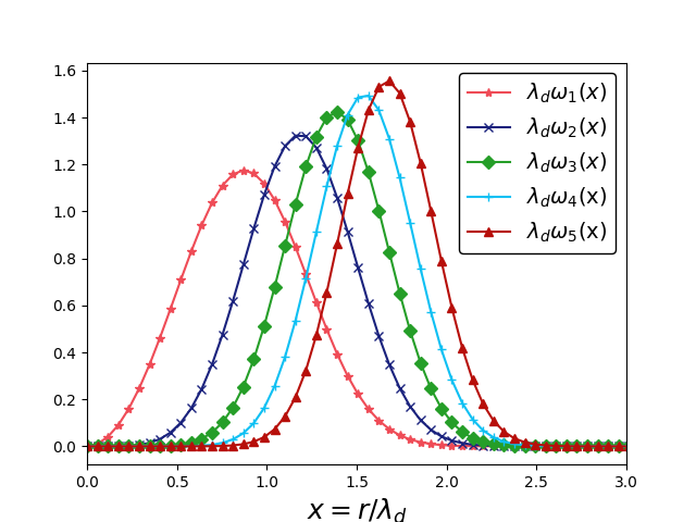
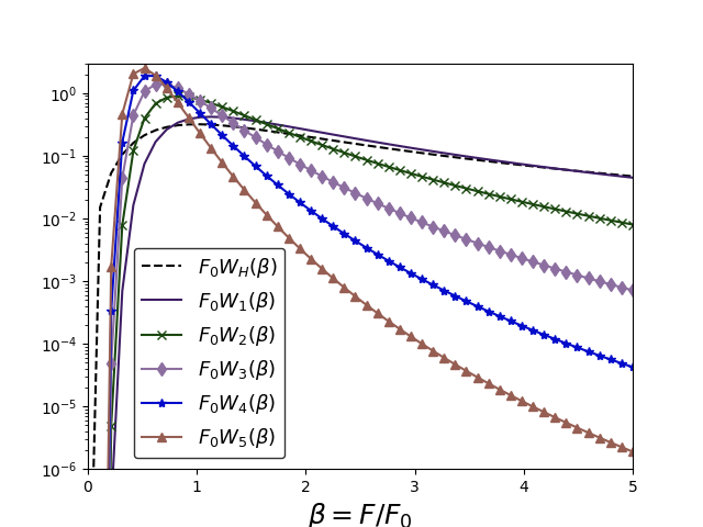
Figure 2: Left - Probability density function $w_{n}(x)$ for finding the $n$-th nearest neighbor at distance $r$ from arbitrary center as a function of the dimensionless variable $x=r/\lambda_{d}$ for dimension $d=3$. Right - Probability density functions $W_{n}(\beta)$ as a function of the normalized force $\beta$.

$W_{n}(F)$ is given by the expression (represented in Figure 2)

$$W_{n}(\beta)=\frac{[5/2\sqrt{2\pi}]^{n}}{F_{0}(n-1)!}\frac{3}{2}\beta^{-(1+3n/2)}\mbox{e}^{-\frac{5\beta^{-3/2}}{2\sqrt{2\pi}}},$$ (105)

where $\beta=F/F_{0}$ and $F_{0}$ the typical force defined in the case of the Holtsmark distribution of force in Eq. (33). The average force modulus $\langle F\rangle_{n}$ is given by

$$\langle F\rangle_{n}=\frac{F_{0}}{(n-1)!}\left(\frac{5}{2\sqrt{2\pi}}\right)^{2/3}\Gamma\left(n-\frac{2}{3}\right).$$ (106)

The average force modulus $\langle F\rangle_{n}$ decreases to 0 when $n$ increases. The moment of order $2$ reaches the following expression for $n>1$ (not finite for $n=1$)

$$\langle F^{2}\rangle_{n}=\frac{F_{0}}{(n-1)!}\left(\frac{5}{2\sqrt{2\pi}}\right)^{4/3}\Gamma\left(n-\frac{4}{3}\right).$$ (107)

More generally, we can show that for $k>2$, the moment of order $k$ is proportional to $\langle F^{k}\rangle_{n}\propto\Gamma(n-2k/3)$ which is finite and positive for $n>2k/3$. The moment of order $k$ converges for $W_{n}(F)$ with $n>2k/3$. The dispersion $\sigma_{W,n}$ is given as follow

$$\sigma_{W,n}=\frac{F_{0}}{\sqrt{(n-1)!}}\left(\frac{5}{2\sqrt{2\pi}}\right)^{2/3}\left[\Gamma\left(n-\frac{4}{3}\right)-\frac{\Gamma(n-2/3)}{(n-1)!}\right]^{1/2}.$$ (108)

We can investigate the case $n=1$ where the distribution of force takes the form

$$W_{1}(F)=\frac{15\beta^{-5/2}}{4\sqrt{2\pi}F_{0}}\exp\left(-\frac{5\beta^{-3/2}}{2\sqrt{2\pi}}\right),$$ (109)

with the average force modulus $\langle F\rangle_{1}$

$$\langle F\rangle_{1}=\left(\frac{5}{2\sqrt{2\pi}}\right)^{2/3}\Gamma\left(\frac{1}{3}\right)F_{0}\approx 2.674F_{0}.$$ (110)

For $F\rightarrow\infty$, reporting the first two terms of the Taylor expansion of $W_{1}(F)$

$$W_{1}(F)\sim\frac{15}{8F_{0}}\left(\frac{2}{\pi}\right)^{1/2}\beta^{-5/2}-\frac{75}{16\pi F_{0}}\beta^{-4}.$$ (111)

We get exactly the first term of the Holtsmark distribution Taylor expansion for $\beta\gg 1$ in equation Eq. (42). That implies that for regime given by $F\rightarrow\infty$, the largest force on the test particle is due to the nearest neighbour. For low $F$, the exponential term cannot admit any Taylor expansion. More generally, for any $n$, we get for $\beta\gg 1$ the Taylor expansion for $W_{n}(F)$

$$W_{n}(\beta) =\frac{[5/2\sqrt{2\pi}]^{n}}{F_{0}(n-1)!}\frac{3}{2}\sum\limits_{k=0}\frac{(-1)^{k}}{k!}\left(\frac{5}{2\sqrt{2\pi}}\right)^{k}\beta^{-(1+3(n+k)/2)}$$ (112)

$$\approx\frac{[5/2\sqrt{2\pi}]^{n}}{F_{0}(n-1)!}\frac{3}{2}\left[\beta^{-(1+3n/2)}-\frac{5}{2\sqrt{2\pi}}\beta^{-(5/2+3n/2)}\right].$$ (113)

At first order, we retrieve for a given index $k$ the exponent of $\beta$ in the series development of the Holtsmark distribution for large $\beta\gg 1$, given by the general term $\beta^{-b_{n}}$ with $b_{n}=1+3n/2$ in equation Eq. (41).

We can write the joint probability to find the set $\{\beta_{i}\}_{1\leq i\leq N}$ knowing the position $r$ of each particle

$$W(\beta_{1},...,\beta_{N}) =\frac{1}{F_{0}^{N}}\frac{dr_{1}...dr_{N}}{d\beta_{1}...d\beta_{N}}w(r_{1},...,r_{N})$$ (114)

$$=\left[\frac{15}{4\sqrt{2\pi}F_{0}}\right]^{N}\prod_{i=1}^{N}\beta_{i}^{-5/2}\mbox{e}^{-\frac{5\beta_{N}^{-3/2}}{2\sqrt{2\pi}}}\widehat{\Theta},$$ (115)

where the Heaviside term $\widehat{\Theta}$ in the density is

$$\widehat{\Theta}=\prod_{i>j=1}^{N}\Theta(\beta_{j}-\beta_{i}).$$ (116)

Considering the new random dimensionless variable $\beta$ as the radial component of the total gravitational force exerted of the center particle following an arbitrary direction

$$\beta=\sum\limits_{i=1}^{N}\beta_{i}\ u_{i},$$ (117)

where $u_{i}=\cos(\theta_{i})$ a random variable distributed uniformly between 1 and $-1$. We note that $\beta_{n}u_{n}$ is the radial coordinate of the contribution $\textbf{F}_{n}$ to the total force F. Giving $u_{i}$ and $\beta_{i}$ independent random variables, the average $\langle\beta\rangle=0$. The statistical distribution for the radial projection of the total gravitational force exerted by a set of $N$ nearest neighbors in dimension $d=3$ is then given by the density $W(\beta)$. We note that the total force modulus is given by the absolute value $|\beta|$, where the distribution $W(|\beta|)$ can be assimilated to the Holtsmark distribution when $N\rightarrow\infty$. We can first calculate the average $\langle\beta^{2}\rangle$, which corresponds exactly to the moment of order 2 of the distribution $W(|\beta|)$. We get

$$\langle\beta^{2}\rangle=\sum\limits_{i,j=1}^{N}\langle\beta_{i}\beta_{j}\rangle\langle u_{i}u_{j}\rangle$$ (118)

where $\langle u_{i}u_{j}\rangle$ is given by $2\delta_{ij}/6$ so we get

$$\langle\beta^{2}\rangle=\frac{2}{6}\sum\limits_{i=1}^{N}\langle\beta_{i}^{2}\rangle=\frac{2}{6}\left[\sum\limits_{i=1}^{N}\left(\frac{\sigma_{W,i}}{F_{0}}\right)^{2}+\langle\beta_{i}\rangle^{2}\right].$$ (119)

Using Eq. (94) for large $N$, the term

$$\sum\limits_{i=1}^{N}\langle\beta_{i}\rangle^{2}\propto\sum\limits_{n=1}^{N}n^{-4/3}$$ (120)

converges for $N$ going to infinity. Also, using the approximation in Eq. (94) and regarding the $n>1$ terms, the sum

$$\sum\limits_{i=2}^{N}(\sigma_{W,i})^{2}\propto\sum\limits_{n=2}^{N}n^{-4/3}\left(1-\frac{n^{2/3}}{(n-1)!}\right)$$ (121)

converges when $N$ is sufficiently large. However, we note that $\langle\beta^{2}\rangle$ diverges to infinity because in the first term of the sum, the dispersion $\sigma_{W_{1}}$ is infinite, regardless the total number of particles $N$. Then, the non-finite dispersion of the distribution $W(|\beta|)$ is due to the first nearest neighbor contribution. For $n>1$, the pair correlation for radial coordinate $\rho(n)$ gets close to 1, the $n$-th nearest neighbors accumulate at equivalent distance and to lower the contribution of the force modulus, whereas the first nearest neighbor is much nearer and exerts in average larger force on the test particle. The fluctuations of the force that follows density $W_{1}(F)$ are also larger than any others and show statistical weights much larger than densities $W_{n>1}(\beta)$ when $\beta\gg 1$.

VII Conclusions

The Holtsmark distribution provides group effect information on the statistics of the gravitational force in a random homogeneous gas with Poisson-like spatial distribution of point particles. We discussed the statistical properties of location in a $d$-dimension space of constant density $\rho_{0}$ of a set of $N$ particles considering the neighborhood of a arbitrary center particle. We generalized the joint probability density function for finding the $N$ nearest neighbors at respective location. Side-by-side particle joint probability density function of location validates that the radial coordinates of 2 nearest neighbor with successive index $n$ are strongly correlated when $n$ is high. In dimension $d=3$, we analyzed the $n$-th contribution to the total gravitational force exerted on a test particle. We noticed that the non-finite dispersion of the Holtsmark distribution is due to the non-finite dispersion of the distribution of force exerted by the first nearest neighbor. We may pursue the study of the gravitational field by using the joint probability distribution for any number of neighbor to investigate the instabilities in a gas of gravitational-bounded particles with homogeneous initial spatial distribution, leading to the emergence of coherent structures (filament). The influence of a continuous mass distribution within the gas may be implemented to the study of statistics of gravitation.

Appendix A Density of location for a particle with finite size

We discuss the statistical properties of the nearest neighbor particle when it has a finite size. For particle with radius $a$, the probability density function to find the nearest neighbour at a distance $r$ has to include a prohibited area of size $r_{\star}=2a$, then

$$w_{1,\star}(r)=\left[1-\int_{r}^{\infty}w_{1,\star}(u)\mbox{d}u\right]G(r)\alpha_{d}r^{d-1}.$$ (122)

The auto correlation function is negative, particle tend to repel each other due to volume exclusion, and expresses as

$$\xi(r)=-\Theta(r_{\star}-r),$$ (123)

where $\Theta$ is the Heaviside function. Giving the same formula as before in Eq. (48), we get the density

$$w_{1,\star}(r)=\Theta(r-r_{\star})N^{\prime}(r)\exp[-N(r)+N(r_{\star})].$$ (124)

The calculus of the average distance $\langle r\rangle_{1,d}^{\star}$ is similar to the previous one, considering the upper incomplete Gamma-Euler function $\Gamma(u,p)$ in Eq. (147), we get

$$\langle r\rangle_{1,d}^{\star} =\int_{0}^{\infty}w_{1,\star}(r)r\mbox{d}r$$ (125)

$$=\lambda_{d}\Gamma\left(\frac{d+1}{d},N(r_{\star})\right)\exp[N(r_{\star})].$$ (126)

We note $u_{\star}=N(r_{\star})$. Giving the expression of $\Gamma(a,x)$

$$\Gamma(a,x)=\Gamma(a)-\gamma(a,x),$$ (127)

where the lower Gamma-Euler function in Eq. (148) admits the Taylor extension for $a>1$

$$\gamma(a,x)=\sum\limits_{n=0}\frac{(-1)^{n}}{n!}\int_{0}^{x}u^{n-1+a}\mbox{d}u=\sum\limits_{n=0}\frac{(-1)^{n}}{n!}\frac{x^{n+a}}{n+a},$$ (128)

with $a=1+1/d>1$. If $x$ is smaller enough, we can consider the first term of the sum

$$\langle r\rangle_{1,d}^{\star}\approx\lambda_{d}\left[\Gamma\left(\frac{d+1}{d}\right)-\frac{d}{d+1}u_{\star}^{1+1/d}\right]\exp[u_{\star}].$$ (129)

By developing the exponential term at first order t, it remains

$$\langle r\rangle_{1,d}^{\star} \approx\lambda_{d}\left[\Gamma\left(\frac{d+1}{d}\right)-\frac{d}{d+1}u_{\star}^{1+1/d}+u_{\star}\Gamma\left(\frac{d+1}{d}\right)\right]$$ (130)

$$\approx\langle r\rangle_{1,d}+u_{\star}\langle r\rangle_{1,d}-\lambda_{d}\frac{d}{d+1}u_{\star}^{1+1/d}.$$ (131)

We introduce the volume fraction $\Phi=\rho_{0}v(r_{\star}/2)$ which is the $N$-sum of each volume occupied by sphere of radius $a=r_{\star}/2$ divided by the volume $V$, it gives

$$\langle r\rangle_{1,d}^{\star}=\langle r\rangle_{1,d}\left[1+2^{d}\Phi\right]-\frac{d}{d+1}2^{d+1}\lambda_{d}\Phi^{1+1/d}.$$ (132)

We note that the modified average distance in the presence of finite size particles is proportional to the average distance calculated with point-like particle with an additional term when the volume fraction $\Phi\ll 1$. We can note that the influence of a finite volume for the $n$-th nearest neighbor for $n>1$ can be neglected when the average distance increases with $n$, because the probability to the $n$-th neighbor particle center within the restricted area defined by the presence of th $n-1$-th neighbor becomes negligible when $n$ is large enough (the approximation is valid when the volume fraction $\Phi\ll 1$).

Appendix B Nearest neighbor probability density function

We can get the same result by considering a finite spherical $d$-volume of radius $R$ given by $v_{d}(R)=\alpha_{d}R^{d}/d$. Let’s note $r$ the radial coordinate of a particle within the sphere and $s=r/R$ the reduced variable comprised between 0 and 1. Considering a free particle in the system, the probability $p(s)ds$ that it is located at $s$ is given by the ratio between the volume of the layer comprised between $r$ and $r+dr$ and the total volume $v_{d}$. We can write

$$p(s)=\left|\frac{\mbox{d}r}{\mbox{d}s}\right|\frac{\alpha_{d}r(s)^{d-1}}{v_{d}}=ds^{d-1}=(s^{d})^{\prime}.$$ (133)

The volume is now filled with $N$ particles with average density $\rho_{0}=N/v_{d}$. For each realization of $N$ particles, we order the positions $\{s_{i}\}_{1\leq i\leq N}$ in a list. Let’s note that the formalism given by the variable $s=r/R$ generalizes the equivalent radius of the system to 1 and makes statistical properties only depending on the total number of particles $N$ within the volume $v_{d}$. It is possible to deduce an evaluation of $w_{n}$ by considering order statistics results. We consider the new random variable $\mathcal{X}$ which corresponds to the $n-$th value of a set of $N$ elements $\{s_{i}\}_{1\leq i\leq N}$ distributed following $p(s)$ and ordered in a list. We define the probability density function $f_{n}$ that verifies the equality

$$\mbox{P}_{n}(\mathcal{X}\in[x,x+\mbox{d}x[)=f_{n}(x)\mbox{d}x.$$ (134)

We can write the general expression for $f_{n}(x)$

$$f_{n}(x) =Kp(x)\left[\int_{0}^{x}p(s)\mbox{d}s\right]^{n-1}\left[\int_{x}^{1}p(s)\mbox{d}s\right]^{N-n}$$ (135)

$$=Kdx^{dn-1}[1-x^{d}]^{N-n}.$$ (136)

With $K$ an appropriated normalization constant. By using the integral in Eq. (152), we derive the final result

$$f_{n}(x)=[nC_{N}^{n}]dx^{dn-1}(1-x^{d})^{N-n}.$$ (137)

Now we investigate the change of variable $x\rightarrow r$ to get the probability density function $w_{n}(r)$ that must verify

$$f_{n}(x)\mbox{d}x=w_{n}(r)\mbox{d}r.$$ (138)

We can express a general form for $w_{n}$ such as:

$$w_{n}(r)=KC_{N}^{n}n\frac{dr^{dn-1}}{R^{dn}}[1-(r/R)^{d}]^{N-n},$$ (139)

where $K$ is a normalization constant associated to the change of space (change from a interval with finite borders $x\in[0,1]$ to an interval with an infinite border $r\in[0,\infty[$). We note that the following expression depends on the two extensive properties of the system $R\ \mbox{and}\ N$. The limit of infinite system $N,R\rightarrow\infty$ and $N/v_{d}=\rho_{0}$ can be considered by developing $1-x\approx\exp[-x]$ when $x=r/R\ll 1$, then

$$w_{n}(r)\approx KC_{N}^{n}n\frac{dr^{dn-1}}{R^{dn}}\exp[-(N-n)(r/R)^{d}].$$ (140)

For $n$ small enough compared to $N$, the difference $N-n\approx N\gg 1$, then we get the exponent

$$(N-n)\left[\frac{r}{R}\right]^{d}\approx\left[\frac{R}{\lambda_{d}}\right]^{d}\left[\frac{r}{R}\right]^{d}=N(r).$$ (141)

The $w_{n}$ density function can be written as

$$w_{n}(r)=\frac{Kd}{(n-1)!}\frac{dr^{dn-1}}{R^{dn}}\mbox{e}^{-N(r)}.$$ (142)

The normalization constant $K$ is given by the integral of $w_{n}$ from 0 to $\infty$, giving $K=(R/\lambda_{d})^{dn}$. The $w_{n}$ function is given by the expression

$$w_{n}(r) =\frac{d}{(n-1)!}\left[\frac{r}{\lambda_{d}}\right]^{dn}\frac{1}{r}\mbox{e}^{-N(r)}$$ (143)

$$=\frac{1}{(n-1)!}N(r)^{n-1}N^{\prime}(r)\mbox{e}^{-N(r)}.$$ (144)

We retrieve the same result as before by considering statistical properties of ordered list elements distributed following the density $p(s)$.

Appendix C Mathematical appendix

The Euler-gamma function given by

$$\Gamma(u)=\int_{0}^{\infty}x^{u-1}\exp(-x)\mbox{d}x.$$ (145)

More generally for the exponents $\alpha$ and $\beta$

$$\Gamma\left(\frac{1+\alpha}{\beta}\right)=\frac{\beta}{K^{1+\alpha}}\int_{0}^{\infty}x^{\alpha}\exp[-(x/K)^{\beta}]\mbox{d}x.$$ (146)

The incomplete upper Euler-gamma function is defined as

$$\Gamma(u,p)=\int_{p}^{\infty}x^{u-1}\exp[-x]\mbox{d}x.$$ (147)

The lower Euler-gamma function is defined as

$$\gamma(u,p)=\Gamma(u)-\Gamma(u,p)=\int_{0}^{p}x^{u-1}\exp(-x)\mbox{d}x.$$ (148)

The Taylor expansion of the $\sin(x)$ function is

$$\sin(x)=\sum\limits_{n=0}\frac{(-1)^{n}}{(2n+1)!}x^{2n+1}.$$ (149)

The Taylor expansion of the $\exp(x)$ function is

$$\exp[x]=\sum\limits_{n=0}\frac{x^{n}}{n!}.$$ (150)

Using the complex integral, we have

$$\int_{0}^{\infty}x^{\alpha}\sin x\mbox{d}x=-\cos\left(\frac{\alpha\pi}{2}\right)\Gamma(1+\alpha).$$ (151)

We give the following Beta integral

$$d\int_{0}^{1}x^{dn-1}(1-x^{d})^{N-n}\mbox{d}x=\frac{\Gamma(N+1-n)\Gamma(n)}{\Gamma(N+1)}.$$ (152)

References

- Chandrasekhar (1943) Chandrasekhar, S. 1943, Rev. Mod. Phys., 15, 1
- Chavanis (2009) Chavanis, P. 2009, The European Physical Journal B volume, 70, 413–433
- Mazur (1992) Mazur, S. 1992, The Journal of Chemical Physics, 97, 9276
- Pietronero et al. (2002) Pietronero, L., Bottaccio, M., Mohayaee, R., & Montuori, M. 2002, Journal of Physics: Condensed Matter, 14, 2141–2152
- Sylos Labini & Pietronero (2008) Sylos Labini, F., & Pietronero, L. 2008, The European Physical Journal B, 64, 615–623