Abstract

We study the problem of parameter estimation for discretely observed stochastic differential equations driven by small fractional noise with Hurst index $H\in(0,1)$. Under some conditions, we obtain strong consistency and rate of convergence of the least square estimator(LSE) when small dispersion coefficient $\varepsilon\rightarrow 0$ and $n\rightarrow\infty$.

1 Introduction

Let $(\Omega,\mathcal{F},(\mathcal{F}_{t}),P)$ be a stochastic basis satisfying the usual conditions. We consider the following stochastic differential equation $X_{t}^{\theta,\varepsilon}$ with an unkown parameter $\theta$

$$\left\{\begin{split}X_{t}^{\theta,\varepsilon}&=\int_{0}^{T}b(\theta,X_{t}^{\theta,\varepsilon})dt+\varepsilon W_{t}^{H}\quad(0\leq t\leq T);\\ X_{0}^{\theta,\varepsilon}&=x_{0}.\end{split}\right.$$ (1.1)

where $x_{0}\in\mathbb{R}$ is a given initial condition, $(W_{t}^{H})$ is a fractional Brownian motion with the given Hurst index $H\in(0,1)$, the true parameter $\theta_{0}$ lies in a certain set $\Theta\subset\mathbb{R}^{d}$ which will be specified later on, $\{b(\cdot,\theta);\theta\in\Theta\}$ is a known family of drift coefficients. The main purpose of this paper is to study the least square type estimator for the true drift parameter $\theta_{0}$ based on the sampling data $(X_{k/n}^{\theta_{0},\varepsilon})_{k=1}^{n}$ with small disperison $\varepsilon>0$ and large sample size $n$.

The asymptotic properties of the maximum likelihood estimator(MLE) for stochastic differential equations driven by the fractional Brownian motion are studied by many authors. (see Kleptsyna and Le Breton [8]; Brouste and Kleptsyna [2]; Tudor and Viens [22]; Rao [20]; Kubilius et al. [9]; Hu et al. [5]; Lohvinenko and Ralchenko [12]; Hu et al. [6]; Tanaka et al. [21] and Chiba [3]) In addition, the strong consistency of LSE for drift parameters is studied by Neuenkirchi and Tindel [18] and the asymptotic normality for discrete observation from the stochastic differential equation driven by the fractional Brownian motion with the Hurst index $H>\frac{1}{2}$ is studied by Nakajima and Shimizu [14].

The parameter estimation problems for diffusion processes with small white noise based o continuous-time observations have been well developed. (see e.g. Kutoyants [10] and [11]; Yoshida [24] and [25]; Uchida and Yoshida [23]) In the case of the small fractional Brownian motion, Nakajima and Shimizu [15] studied the asymptotic properties of MLE based on continuous-time observations. However, to the best of the authors’ knowledge, parameter estimation problems on the discrete observation from the stochastic differential equation driven by small fractional Brownian motion have not been studied. Therefore, in this paper, we studied the asymptotic properties of LSE for discretely observed diffusion processes with small fractional Brownian motion with Hurst index $H\in(0,1)$ when $\varepsilon\rightarrow 0,n\rightarrow\infty$. The main tool to obtain the asymptotic properties of estimators is an inequality evaluation of the stochastic integral by Young inequality for the Young integral. (see Young [26]) Since we can evaluate the stochastic integral at each point by Young inequality, we obtain strong consistency and asymptotic normality in the sense of almost surely convergence.

This paper is organized as follows. In Section 2, we state our main results and prepare some auxiliary results for the proofs of our main results. All the proofs are given in Section 3. In Section 4, we provide some simulation studies to confirm our main results.

2 Main results

In this section, we investigate our main results. Using high frequency data $(X_{t_{i}}^{\theta,\varepsilon})_{i=1}^{n}$ with $t_{i+1}-t_{i}=\frac{1}{n}$, the contrast function $L_{\varepsilon,n}(\theta)$ is defined as follows

$$Q_{\varepsilon,n}(\theta) :=n\sum_{k=0}^{n-1}\left|\delta X_{t_{k}t_{k+1}}^{\theta_{0},\varepsilon}-\frac{1}{n}b(X_{t_{k}}^{\theta_{0},\varepsilon},\theta)\right|^{2},$$

$$L_{\varepsilon,n}(\theta) :=Q_{\varepsilon,n}(\theta)-Q_{\varepsilon,n}(\theta_{0}),$$

where $\delta X_{t_{k}t_{k+1}}^{\theta_{0},\varepsilon}=X_{t_{k+1}}^{\theta_{0},\varepsilon}-X_{t_{k}}^{\theta_{0},\varepsilon}$. Then, the LSE $\hat{\theta}_{n,\varepsilon}$ is defined as

$$\hat{\theta}_{n,\varepsilon}:=\underset{\theta\in\Theta}{\text{argmin}}L_{n,\varepsilon}^{\alpha}(\theta).$$

Our interest in this paper is to obtain the asymptotic properties of $\hat{\theta}_{n,\varepsilon}$.

To state our main results, we make some notations. Let $(x_{t}^{\theta})_{0\leq t\leq T}$ be the solution to the underlying ordinary differential equation (ODE) under the true value of the drift parameter:

$$\left\{\begin{split}dx_{t}^{\theta}&=b\left(x_{t}^{\theta},\theta\right)dt,\\ x_{0}^{\theta}&=x_{0}.\end{split}\right.$$

We denote the space of all functions $f:\mathbb{R}\times\Theta\rightarrow\mathbb{R}$ which is $k$ and $l$ times continuous differentiable by $C^{k,l}(\mathbb{R},\Theta)$. Moreover $C_{\uparrow}^{k,l}(\mathbb{R},\Theta)$ is a class of $f\in C^{k,l}(\mathbb{R},\Theta)$ satisfying that $\underset{\theta\in\Theta}{\sup}\left|\partial_{x}\partial_{\theta_{i}}f(x,\theta)\right|\leq C(1+\left|x\right|^{\lambda})$ for universal positive constants $C$ and $\lambda$, where $\theta_{i}$ is the $i$-th projection of $\theta$.

We introduce the following assumptions.

• $\Theta$ is an open bounded convec subset of $\mathbb{R}^{d}$.

• $\theta\neq\theta_{0}$ $\leftrightarrow$ $b(x_{t}^{\theta_{0}},\theta)\neq b(x_{t}^{\theta_{0}},\theta_{0})$ for at least one value of $t\in[0,1]$.

• There exists a constant $c>0$ such that

  $$\underset{\theta\in\Theta}{\sup}\left|b(x,\theta)-b(y,\theta)\right| \leq c\left|x-y\right|,$$

  $$\underset{\theta\in\Theta}{\sup}\left|\partial_{x}b(x,\theta)-\partial_{x}b(y,\theta)\right| \leq c\left|x-y\right|,$$

  $$\left|b(x,\theta_{1})-b(x,\theta_{2})\right| \leq c\left(1+\left|x\right|^{N}\right)\left|\theta_{1}-\theta_{2}\right|,$$

  $$\underset{\theta\in\Theta}{\sup}\left|b(x,\theta)\right| \leq c\left(1+|x|\right),$$

  for each $x\in\mathbb{R}$ , $N\in\mathbb{N}$ and $\theta_{1},\theta_{2}\in\Theta$.

• $b(\cdot,\cdot)\in C_{\uparrow}^{2,3}\left(\mathbb{R},\Theta\right)$.

• $I(\theta_{0})=\left(I^{i,j}(\theta_{0})\right)_{1\leq i,j\leq d}$ is positive definite, where

  $$I^{i,j}(\theta):=\int_{0}^{1}\left(\partial_{\theta_{i}}b\left(x_{s}^{\theta_{0}},\theta\right)\right)^{\top}\partial_{\theta_{j}}b\left(x_{s}^{\theta_{0}},\theta\right)ds.$$

Theorem 1.

Suppose that (A1)–(A3) and either of the following conditions hold:

• $H>\frac{1}{2}$.

• $H\leq\frac{1}{2}$ and $\varepsilon^{2}n^{1-H}\rightarrow 0\quad(n\rightarrow\infty,\varepsilon\downarrow 0)$.

Then we have $\hat{\theta}_{n,\varepsilon}\rightarrow\theta_{0}\ \text{a.s.}\quad(n\rightarrow\infty,\varepsilon\downarrow 0)$.

Theorem 2.

Suppose that (A1)–(A5) and either of the following conditions holds:

• $H>\frac{1}{2}$ and $\varepsilon n\rightarrow\infty.$

• $H\leq\frac{1}{2}$, $\varepsilon n^{1-H}\rightarrow 0$ and $\varepsilon n\rightarrow\infty.$

Then we have

$$\varepsilon^{-1}\left(\hat{\theta}_{n,\varepsilon}-\theta_{0}\right)\rightarrow I^{-1}(\theta_{0})S(\theta_{0})\quad\text{a.s.}\quad(n\rightarrow\infty,\varepsilon\downarrow 0),$$ (2.1)

where

$$I(\theta_{0}) :=\left(\int_{0}^{T}\partial_{\theta_{i}}b\left(x_{s}^{\theta_{0}},\theta_{0}\right)\partial_{\theta_{j}}b\left(x_{s}^{\theta_{0}},\theta_{0}\right)ds\right)_{1\leq i,j\leq d},$$

$$S(\theta_{0}) :=\left(\int_{0}^{T}\partial_{\theta_{i}}b\left(x_{s}^{\theta_{0}},\theta_{0}\right)dW_{s}^{H}\right)_{1\leq i,j\leq d}.$$

Remark 1.

The stochastic integral $S(\theta_{0}):=\int_{0}^{T}\partial_{\theta_{i}}b\left(x_{s}^{\theta_{0}},\theta_{0}\right)dW_{s}^{H}$ is defined as Young integral. (see Young [26]) When $H=1/2$, $S(\theta_{0})$ is coincide with the Itô integral.

3 Proof

3.1 Auxiliary results

We shall prepare a stochastic integral for fractional Brownian motion and its properties. Let $C_{\lambda}(A)$ be the space of all functions $f:A\rightarrow\mathbb{R}$ which is $\lambda$-Hölder continuous function. It is well known that the Riemann-Stieltjes integral $\int_{a}^{b}f(t)dg(t)$ exists for any $f\in C_{p}([a,b])$ and $g\in C_{q}([a,b])$ with $p+q>1$. (see Young [26]) Also, the the change of variable is valid as the following. (see Zähle [27])

Lemma 1.

Let $f\in C_{p}([a,b])$ with $p>\frac{1}{2}$ and $F\in C^{1}(\mathbb{R})$. Then we have

$$F\left(f(y)\right)-F\left(f(a)\right)=\int_{a}^{y}F^{\prime}\left(f(t)\right)df(t),$$

for any $y\in[a,b]$.

For estimating the Young integral, we note the following estimate, which can be found e.g. in Young [26].

Lemma 2.

Let $f\in C_{\lambda}([a,b])$ and $g\in C_{\mu}([a,b])$ with $\lambda+\mu>1$. Then, there exists a constant $c_{\lambda,\mu}$ such that

$$\left|\int_{a}^{b}\left(f(s)-f(a)\right)dg(s)\right|\leq c_{\lambda,\mu}\left\|f\right\|_{\lambda;[a,b]}\left\|g\right\|_{\mu;[a,b]}|b-a|^{\lambda;\mu},$$

where $\|\cdot\|_{\lambda;[a,b]}$ is the Hölder norm on $C_{\lambda}([a,b])$.

3.2 Proof of the strong consistency

We consider the following proposition which is the convergence of the contrast function $L_{n,\varepsilon}(\theta)$ uniformly with respect to $\theta\in\Theta$.

Proposition 1.

Suppose that (A1)–(A3) and $\varepsilon^{2}n^{\left(1-H\right)}\rightarrow 0\quad(n\rightarrow\infty,\varepsilon\downarrow 0)$ hold.Then we have

$$\underset{\theta\in\Theta}{\sup}\left|Q_{n,\varepsilon}(\theta)-Q_{n,\varepsilon}(\theta_{0})-\int_{0}^{T}\left|b(x_{s}^{\theta_{0}},\theta)-b(x_{s}^{\theta_{0}},\theta_{0})\right|^{2}ds\right|\rightarrow 0\quad\left(n\rightarrow\infty,\varepsilon\downarrow 0\right).$$

Lemma 3.

Under a assumption (A3), for any $\theta\in\Theta$ and $0\leq t\leq T$, we have

$$\underset{\begin{subarray}{c}\theta\in\Theta\\ 0\leq t\leq T\end{subarray}}{\sup}\left|X_{t}^{\theta,\varepsilon}-x_{t}^{\theta,\varepsilon}\right|\leq\varepsilon e^{cT}\underset{0\leq t\leq T}{\sup}\left|W_{t}^{H}\right|.$$

In particular,

$$\underset{\begin{subarray}{c}\theta\in\Theta\\ 0\leq t\leq T\end{subarray}}{\sup}\left|X_{t}^{\theta,\varepsilon}-x_{t}^{\theta,\varepsilon}\right|\rightarrow 0\quad(\varepsilon\downarrow 0).$$

Proof.

For any $\theta\in\Theta$ and $0\leq t\leq T$, we have

$$\left|X_{t}^{\theta,\varepsilon}-x_{t}^{\theta,\varepsilon}\right| \leq\int_{0}^{t}\left|b\left(X_{s}^{\theta,\varepsilon},\theta\right)-b\left(x_{s}^{\theta,\varepsilon},\theta\right)\right|ds+\varepsilon\left|W_{t}^{H}\right|$$

$$\leq c\int_{0}^{t}\left|X_{s}^{\theta,\varepsilon}-x_{s}^{\varepsilon}\right|ds+\varepsilon\underset{0\leq t\leq T}{\sup}\left|W_{t}^{H}\right|.$$

By Gronwall’s inequality, it follows that

$$\underset{\theta\in\Theta}{\sup}\left|X_{t}^{\theta,\varepsilon}-x_{t}^{\theta,\varepsilon}\right|\leq\varepsilon e^{ct}\underset{0\leq t\leq T}{\sup}\left|W_{t}^{H}\right|.$$

Thus we obtain the first estimate and this proof is completed. ∎

Lemma 4.

Under assumptions (A1) and (A3), we have

$$Q_{n,\varepsilon}(\theta)-Q_{n,\varepsilon}(\theta_{0})=Q_{n,\varepsilon}^{(1)}(\theta)-2Q_{n,\varepsilon}^{(2)}(\theta)+R_{n,\varepsilon}(\theta),$$ (3.1)

where

$$Q_{n,\varepsilon}^{(1)}(\theta) :=\frac{1}{n}\sum_{k=0}^{n-1}\left|b(X_{t_{k}}^{\theta_{0},\varepsilon},\theta)-b(X_{t_{k}}^{\theta_{0},\varepsilon},\theta_{0})\right|^{2},$$

$$Q_{n,\varepsilon}^{(2)}(\theta) :=\sum_{k=0}^{n-1}\left(b(X_{t_{k}}^{\theta_{0},\varepsilon},\theta)-b(X_{t_{k}}^{\theta_{0},\varepsilon},\theta_{0})\right)\left(\varepsilon\left(W_{t_{k+1}}^{H}-W_{t_{k}}^{H}\right)\right),$$

$$R_{n,\varepsilon}(\theta) :=-2\sum_{k=0}^{n-1}\left(b(X_{t_{k}}^{\theta_{0},\varepsilon},\theta)-b(X_{t_{k}}^{\theta_{0},\varepsilon},\theta_{0})\right)\int_{t_{k}}^{t_{k+1}}\left(b(X_{s}^{\theta_{0},\varepsilon},\theta_{0})-b(X_{t_{k}}^{\theta_{0},\varepsilon},\theta_{0})\right)ds.$$

In particular, we have

$$\underset{\theta\in\Theta}{\sup}\left|R_{n,\varepsilon}(\theta)\right|\rightarrow 0\quad\text{a.s.}\quad(n\rightarrow\infty,\varepsilon\downarrow 0).$$

Proof.

(3.1) is follows that

$$\frac{1}{n}\left(Q_{n,\varepsilon}^{\alpha}(\theta)-Q_{n,\varepsilon}^{\alpha}(\theta_{0})\right)$$

$$=\sum_{k=0}^{n-1}\left\{\left|\delta X_{t_{k}t_{k+1}}^{\theta_{0},\varepsilon}-\frac{1}{n}b(X_{t_{k}}^{\theta_{0},\varepsilon},\theta)\right|^{2}-\left|\delta X_{t_{k}t_{k+1}}^{\theta_{0},\varepsilon}-\frac{1}{n}b(X_{t_{k}}^{\theta_{0},\varepsilon},\theta_{0})\right|^{2}\right\}$$

$$=-2\frac{1}{n}\sum_{k=0}^{n-1}\left(b(X_{t_{k}}^{\theta_{0},\varepsilon},\theta)-b(X_{t_{k}}^{\theta_{0},\varepsilon},\theta_{0})\right)\delta X_{t_{k}t_{k+1}}^{\theta_{0},\varepsilon}+\left(\frac{1}{n}\right)^{2}\sum_{k=0}^{n-1}\left(b(X_{t_{k}}^{\theta_{0},\varepsilon},\theta)^{2}-b(X_{t_{k}}^{\theta_{0},\varepsilon},\theta_{0})^{2}\right)$$

$$=-2\frac{1}{n}\sum_{k=0}^{n-1}\left(b(X_{t_{k}}^{\theta_{0},\varepsilon},\theta)-b(X_{t_{k}}^{\theta_{0},\varepsilon},\theta_{0})\right)\left(\delta X_{t_{k}t_{k+1}}^{\theta_{0},\varepsilon}-\frac{1}{n}b(X_{t_{k}}^{\theta_{0},\varepsilon},\theta_{0})\right)+\left(\frac{1}{n}\right)^{2}\sum_{k=0}^{n-1}\left(b(X_{t_{k}}^{\theta_{0},\varepsilon},\theta)-b(X_{t_{k}}^{\theta_{0},\varepsilon},\theta_{0})\right)^{2}$$

$$=\frac{1}{n}\left(Q_{n,\varepsilon}^{\alpha,(1)}(\theta)+Q_{n,\varepsilon}^{\alpha,(2)}(\theta)+R_{n+\varepsilon}(\theta)\right).$$

Since the path of the fractional Brownian motion $(W_{t}^{H})_{t\in[0,T]}$ is $\nu$-Hölder continuous for any $\nu\in(0,H)$, we obtain

$$\left|X_{t}^{\theta_{0},\varepsilon}-X_{s}^{\theta_{0},\varepsilon}\right| \leq\int_{s}^{t}\left|b\left(X_{u}^{\theta_{0},\varepsilon},\theta_{0}\right)\right|du+\varepsilon\left(W_{t}^{H}-W_{s}^{H}\right)$$

$$\leq\left(t-s\right)\left\{1+\left(\varepsilon e^{cT}\underset{0\leq t\leq T}{\sup}\left|W_{t}^{H}\right|+\underset{0\leq t\leq T}{\sup}\left|x_{t}^{\theta_{0}}\right|\right)^{N}\right\}+\varepsilon\left(t-s\right)^{\lambda},$$ (3.2)

for any $\lambda\in(0,H)$. From (3.2), we have

$$\underset{\theta\in\Theta}{\sup}\left|R_{n,\varepsilon}(\theta)\right|$$

$$=\underset{\theta\in\Theta}{\sup}\left|2\sum_{k=0}^{n-1}\left(b\left(X_{t_{k}}^{\varepsilon,\theta_{0}},\theta\right)-b\left(X_{t_{k}}^{\theta_{0},\varepsilon},\theta_{0}\right)\right)\left(\int_{t_{k}}^{t_{k+1}}b\left(X_{s}^{\theta_{0},\varepsilon},\theta_{0}\right)-b\left(X_{t_{k}}^{\theta_{0},\varepsilon},\theta_{0}\right)ds\right)\right|$$

$$\lesssim\left\{1+\left(\varepsilon e^{cT}\underset{0\leq t\leq T}{\sup}\left|W_{t}^{H}\right|+\underset{0\leq t\leq T}{\sup}\left|x_{t}^{\theta_{0}}\right|\right)^{N}\right\}$$

$$\times\sum_{k=0}^{n-1}\left[\int_{t_{k}}^{t_{k+1}}\left(t_{k+1}-t_{k}\right)\left\{1+\left(\varepsilon e^{cT}\underset{0\leq t\leq T}{\sup}\left|W_{t}^{H}\right|+\underset{0\leq t\leq T}{\sup}\left|x_{t}^{\theta_{0}}\right|\right)^{N}\right\}+\varepsilon\left(t_{k+1}-t_{k}\right)^{\lambda}ds\right]$$

$$=\left\{1+\left(\varepsilon e^{cT}\underset{0\leq t\leq T}{\sup}\left|W_{t}^{H}\right|+\underset{0\leq t\leq T}{\sup}\left|x_{t}^{\theta_{0}}\right|\right)^{N}\right\}\left[\frac{1}{n}\left\{1+\left(\varepsilon e^{cT}\underset{0\leq t\leq T}{\sup}\left|W_{t}^{H}\right|+\underset{0\leq t\leq T}{\sup}\left|x_{t}^{\theta_{0}}\right|\right)^{N}\right\}+\varepsilon\left(\frac{1}{n}\right)^{\lambda}\right]$$

$$\rightarrow 0\quad(n\rightarrow\infty,\varepsilon\downarrow 0).$$

∎

Lemma 5.

Let $H\in(0,1)$ and $f\in C_{\uparrow}^{1,1}(\mathbb{R},\Theta)$. Then we have

$$\underset{\theta\in\Theta}{\sup}\left|\frac{1}{n}\sum_{k=0}^{n-1}f(X_{t_{k}}^{\theta_{0},\varepsilon},\theta)-\int_{0}^{T}f(x_{s}^{\theta_{0}},\theta)\right|\rightarrow 0\quad\text{a.s.}\quad(n\rightarrow\infty,\varepsilon\downarrow 0).$$

In particular, under assumptions (A1) and (A3), we obtain

$$\underset{\theta\in\Theta}{\sup}\left|Q_{n,\varepsilon}^{\alpha,(1)}(\theta)-\int_{0}^{T}\left|b(x_{s}^{\theta_{0}},\theta)-b(x_{s}^{\theta_{0}},\theta_{0})\right|^{2}ds\right|\rightarrow 0\quad\text{a.s.}\quad(n\rightarrow\infty,\varepsilon\downarrow 0).$$

Proof.

For proof, see Hu et al. [13], Lemma 3.3. ∎

Lemma 6.

Let $H\in(0,1)$ and $f\in C_{\uparrow}^{1,1}(\mathbb{R},\Theta)$ such that $\underset{\theta\in\Theta}{\sup}\left|f(x,\theta)-f(y,\theta)\right|\leq c\left|x-y\right|$. Suppose that $\varepsilon n^{\left(1-H\right)}\rightarrow 0\quad(n\rightarrow\infty,\varepsilon\downarrow 0)$ holds, then we have

$$\underset{\theta\in\Theta}{\sup}\left|\sum_{k=0}^{n-1}f(X_{t_{k}}^{\theta_{0},\varepsilon},\theta)(W_{t_{k+1}}^{H}-W_{t_{k}}^{H})-\int_{0}^{T}f(x_{s}^{\theta_{0}},\theta)dW_{s}^{H}\right|\rightarrow 0\quad\text{a.s.}\quad(n\rightarrow\infty,\varepsilon\downarrow 0).$$

In addition, (A3) and $\varepsilon^{2}n^{\left(1-H\right)}\rightarrow 0\quad(n\rightarrow\infty,\varepsilon\downarrow 0)$ hold , then we obtain

$$\underset{\theta\in\Theta}{\sup}\left|Q_{n,\varepsilon}^{\alpha,(2)}(\theta)\right|\rightarrow 0\quad\text{a.s.}\quad(n\rightarrow\infty,\varepsilon\downarrow 0).$$

Proof.

For any $\lambda\in(1-H,1),\lambda^{\prime}\in(0,H)$ s.t. $\lambda+\lambda^{\prime}>1$, we have

$$\underset{\theta\in\Theta}{\sup}\left|\sum_{k=0}^{n-1}f(X_{t_{k}}^{\theta_{0},\varepsilon},\theta)(W_{t_{k+1}}^{H}-W_{t_{k}}^{H})-\int_{0}^{T}f(x_{s}^{\theta_{0}},\theta)dW_{s}^{H}\right|$$

$$\leq\underset{\theta\in\Theta}{\sup}\left|\sum_{k=0}^{n-1}f(X_{t_{k}}^{\theta_{0},\varepsilon},\theta)(W_{t_{k+1}}^{H}-W_{t_{k}}^{H})-\sum_{k=0}^{n-1}f(x_{t_{k}}^{\theta_{0}},\theta)(W_{t_{k+1}}^{H}-W_{t_{k}}^{H})\right|$$

$$+\underset{\theta\in\Theta}{\sup}\left|\sum_{k=0}^{n-1}f(x_{t_{k}}^{\theta_{0}},\theta)(W_{t_{k+1}}^{H}-W_{t_{k}}^{H})-\int_{0}^{T}f(x_{s}^{\theta_{0}},\theta)dW_{s}^{H}\right|$$

$$\leq\underset{\theta\in\Theta}{\sup}\left\{\left(\sum_{k=0}^{n-1}\left|f\left(X_{t_{k}}^{\theta_{0},\varepsilon},\theta\right)-f\left(x_{t_{k}}^{\theta_{0}},\theta\right)\right|^{\frac{1}{1-H}}\right)^{1-H}\left(\sum_{k=0}^{n-1}\left|W_{t_{k+1}}^{H}-W_{t_{k}}^{H}\right|^{\frac{1}{H}}\right)^{H}\right\}$$

$$+\sum_{k=0}^{n-1}\underset{\theta\in\Theta}{\sup}\left|\int_{t_{k}}^{t_{k+1}}f(x_{t_{k}}^{\theta_{0}},\theta)-f(x_{s}^{\theta_{0}},\theta)dW_{s}^{H}\right|$$

$$\uwave{<}n^{1-H}\underset{0\leq t\leq T}{\sup}\left|X_{t}^{\theta_{0},\varepsilon}-x_{t}^{\theta_{0}}\right|\left(\sum_{k=0}^{n-1}\left|W_{t_{k+1}}^{H}-W_{t_{k}}^{H}\right|^{\frac{1}{H}}\right)^{H}+\sum_{k=0}^{n-1}\underset{\theta\in\Theta}{\sup}\left\|f\left(x_{\cdot}^{\theta_{0}},\theta\right)\right\|_{\lambda;[t_{k},t_{k+1}]}\left\|W_{\cdot}^{H}\right\|_{\lambda^{\prime};[t_{k},t_{k+1}]}\left(\frac{1}{n}\right)^{\lambda+\lambda^{\prime}}$$

$$\lesssim\varepsilon n^{1-H}\left(\sum_{k=0}^{n-1}\left|W_{t_{k+1}}^{H}-W_{t_{k}}^{H}\right|^{\frac{1}{H}}\right)^{H}+n\left(\frac{1}{n}\right)^{1-\lambda}\left(\frac{1}{n}\right)^{H-\lambda^{\prime}}\left(\frac{1}{n}\right)^{\lambda+\lambda^{\prime}}$$

$$=\varepsilon n^{1-H}\left(\sum_{k=0}^{n-1}\left|W_{t_{k+1}}^{H}-W_{t_{k}}^{H}\right|^{\frac{1}{H}}\right)^{H}+\left(\frac{1}{n}\right)^{H}$$

$$\rightarrow 0\quad(n\rightarrow\infty,\varepsilon\downarrow 0).$$

by Lemma 2, Neuenkirch and Tindel [18], Lemma2.5 and Lemma 2.6. ∎

Lemma 7.

Let $H>\frac{1}{2}$ and $f\in C_{\uparrow}^{1,1}(\mathbb{R}\Theta)$ such taht

$$\underset{\theta\in\Theta}{\sup}\left|f\left(x,\theta\right)-f\left(y,\theta\right)\right| \leq c\left|x-y\right|,$$

$$\underset{\theta\in\Theta}{\sup}\left|\partial_{x}f\left(x,\theta\right)-\partial_{x}f\left(y,\theta\right)\right| \leq c\left|x-y\right|.$$

Then we have

$$\underset{\theta\in\Theta}{\sup}\left|\sum_{k=0}^{n-1}f\left(X_{t_{k}}^{\theta_{0},\varepsilon},\theta\right)\left(W_{t_{k+1}}^{H}-W_{t_{k}}^{H}\right)-\int_{0}^{T}f(x_{t}^{\theta_{0}}\theta)dW_{t}^{H}\right|\rightarrow 0\quad\text{a.s.}\quad(n\rightarrow\infty,\varepsilon\downarrow 0).$$ (3.3)

In particular, under the assumptions (A1) and (A4), we obtain

$$\underset{\theta\in\Theta}{\sup}\left|Q_{n,\varepsilon}^{\alpha,(2)}(\theta)\right|\rightarrow 0\quad\text{a.s.}\quad(n\rightarrow\infty,\varepsilon\downarrow 0).$$

Proof.

Let $\lambda\in(0,H)$ such that $2\lambda>1$.

$$\underset{\theta\in\Theta}{\sup}\left|\sum_{k=0}^{n-1}f\left(X_{t_{k}}^{\theta_{0},\varepsilon},\theta\right)\left(W_{t_{k+1}}^{H}-W_{t_{k}}^{H}\right)-\int_{0}^{T}f\left(x_{t}^{\theta_{0}},\theta\right)dW_{t}^{H}\right|$$

$$\leq\underset{\theta\in\Theta}{\sup}\left|\sum_{k=0}^{n-1}f\left(X_{t_{k}}^{\theta_{0},\varepsilon},\theta\right)\left(W_{t_{k+1}}^{H}-W_{t_{k}}^{H}\right)-\int_{0}^{T}f\left(X_{t}^{\theta_{0},\varepsilon},\theta\right)dW_{t}^{H}\right|+\underset{\theta\in\Theta}{\sup}\left|\int_{0}^{T}f\left(X_{t}^{\theta_{0},\varepsilon},\theta\right)dW_{t}^{H}-\int_{0}^{T}f\left(x_{t}^{\theta_{0}},\theta\right)dW_{t}^{H}\right|$$

$$=\underset{\theta\in\Theta}{\sup}\left|\sum_{k=0}^{n-1}\int_{t_{k}}^{t_{k+1}}\left\{f\left(X_{t_{k}}^{\theta_{0},\varepsilon},\theta\right)-f\left(X_{t}^{\theta_{0},\varepsilon},\theta\right)\right\}dW_{t}^{H}\right|$$

$$+\underset{\theta\in\Theta}{\sup}\left|\int_{0}^{T}\left\{f\left(X_{t}^{\theta_{0},\varepsilon},\theta\right)-f\left(x_{t}^{\theta_{0}},\theta\right)-\left(f\left(x_{0}^{\theta_{0}},\theta\right)-f\left(x_{0}^{\theta_{0}},\theta\right)\right)\right\}dW_{t}^{H}\right|$$

$$\leq\sum_{k=0}^{n-1}\underset{\theta\in\Theta}{\sup}\left\|f\left(X_{\cdot}^{\theta_{0},\varepsilon},\theta\right)\right\|_{\lambda;[t_{k},t_{k+1}]}\left\|W_{\cdot}^{H}\right\|_{\lambda;[t_{k},t_{k+1}]}\left(\frac{1}{n}\right)^{2\lambda}+\underset{\theta\in\Theta}{\sup}\left\|f\left(X_{\cdot}^{\theta_{0},\varepsilon},\theta\right)-f\left(x_{\cdot}^{\theta_{0}},\theta\right)\right\|_{\lambda;[0,T]}\left\|W_{\cdot}^{H}\right\|_{\lambda;[0,T]}T^{2\lambda}$$

$$\lesssim\sum_{k=0}^{n-1}\left[\left\{1+\left(\varepsilon e^{cT}\underset{0\leq t\leq T}{\sup}\left|W_{t}^{H}\right|+\underset{0\leq t\leq T}{\sup}\left|x_{t}^{\theta_{0}}\right|\right)^{N}\right\}\left(\frac{1}{n}\right)^{1-\lambda}+\varepsilon\left\|W_{\cdot}^{H}\right\|_{\lambda;[t_{k},t_{k+1}]}\right]\left\|W_{\cdot}^{H}\right\|_{\lambda;[t_{k},t_{k+1}]}\left(\frac{1}{n}\right)^{2\lambda}$$

$$+\underset{\theta\in\Theta}{\sup}\left\|f\left(X_{\cdot}^{\theta_{0},\varepsilon},\theta\right)-f\left(x_{\cdot}^{\theta_{0}},\theta\right)\right\|_{\lambda;[0,T]}\left\|W_{\cdot}^{H}\right\|_{\lambda;[0,T]}T^{2\lambda}$$

$$\lesssim\left[\left\{1+\left(\varepsilon e^{cT}\underset{0\leq t\leq T}{\sup}\left|W_{t}^{H}\right|+\underset{0\leq t\leq T}{\sup}\left|x_{t}^{\theta_{0}}\right|\right)^{N}\right\}\left(\frac{1}{n}\right)^{H}+\varepsilon\left(\frac{1}{n}\right)^{2H-1}\right]$$

$$+\underset{\theta\in\Theta}{\sup}\left\|f\left(X_{\cdot}^{\theta_{0},\varepsilon},\theta\right)-f\left(x_{\cdot}^{\theta_{0}},\theta\right)\right\|_{\lambda;[0,T]}\left\|W_{\cdot}^{H}\right\|_{\lambda;[0,T]}T^{2\lambda}.$$ (3.4)

Note that

$$f\left(X_{t}^{\theta_{0},\varepsilon},\theta\right)-f\left(x_{0},\theta\right) =\int_{0}^{t}\partial_{x}f\left(X_{s}^{\theta_{0},\varepsilon},\theta\right)dX_{s}^{\theta_{0},\varepsilon}$$

$$=\int_{0}^{t}\partial_{x}f\left(X_{s}^{\theta_{0},\varepsilon},\theta\right)b\left(X_{s}^{\theta_{0},\varepsilon},\theta_{0}\right)ds+\varepsilon\int_{0}^{t}\partial_{x}f\left(X_{s}^{\theta_{0},\varepsilon},\theta\right)dW_{s}^{H},$$

and

$$f\left(x_{t}^{\theta_{0}},\theta\right)-f\left(x_{0},\theta\right)=\int_{0}^{t}\partial_{x}f\left(x_{s}^{\theta_{0}},\theta\right)b\left(x_{s}^{\theta_{0}},\theta_{0}\right)ds,$$

hold from Lemma 2. Thus, we have

$$\left|f\left(X_{t}^{\theta_{0},\varepsilon},\theta\right)-f\left(x_{t}^{\theta_{0}},\theta\right)-\left(f\left(X_{s}^{\theta_{0},\varepsilon},\theta\right)-f\left(x_{s}^{\theta_{0}},\theta\right)\right)\right|$$

$$\leq\left|\int_{s}^{t}\left\{\partial_{x}f\left(X_{u}^{\theta_{0},\varepsilon},\theta\right)b\left(X_{u}^{\theta_{0},\varepsilon},\theta_{0}\right)-\partial_{x}f\left(x_{u}^{\theta_{0}},\theta\right)b\left(x_{u}^{\theta_{0}},\theta_{0}\right)\right\}du\right|+\varepsilon\left|\int_{s}^{t}f\left(X_{u}^{\theta_{0},\varepsilon},\theta\right)dW_{u}^{H}\right|$$

$$\leq\left|\int_{s}^{t}\left\{\partial_{x}f\left(X_{u}^{\theta_{0},\varepsilon},\theta\right)b\left(X_{u}^{\theta_{0},\varepsilon},\theta_{0}\right)-\partial_{x}f\left(x_{u}^{\theta_{0}},\theta\right)b\left(X_{u}^{\theta_{0},\varepsilon},\theta_{0}\right)\right\}du\right|$$

$$+\left|\int_{s}^{t}\left\{\partial_{x}f\left(x_{u}^{\theta_{0}},\theta\right)b\left(X_{u}^{\theta_{0},\varepsilon},\theta_{0}\right)-\partial_{x}f\left(x_{u}^{\theta_{0}},\theta\right)b\left(x_{u}^{\theta_{0}},\theta_{0}\right)\right\}du\right|$$

$$+\varepsilon\left|\int_{s}^{t}f\left(X_{u}^{\theta_{0},\varepsilon},\theta\right)-f\left(X_{s}^{\theta_{0},\varepsilon},\theta\right)dW_{u}^{H}\right|+\varepsilon\left|f\left(X_{s}^{\theta_{0},\varepsilon},\theta\right)\left(W_{t}^{H}-W_{s}^{H}\right)\right|$$

$$\uwave{<}\left(t-s\right)\left(1+\underset{0\leq t\leq T}{\sup}\left|X_{t}^{\theta_{0},\varepsilon}\right|^{N}\right)\underset{0\leq t\leq T}{\sup}\left|X_{t}^{\theta_{0},\varepsilon}-x_{t}^{\theta_{0}}\right|+(t-s)\left(1+\underset{0\leq t\leq T}{\sup}\left|x_{t}^{\theta_{0}}\right|^{N}\right)\underset{0\leq t\leq T}{\sup}\left|X_{t}^{\theta_{0},\varepsilon}-x_{t}^{\theta_{0}}\right|$$

$$+\varepsilon\left\|f\left(X_{\cdot}^{\theta_{0},\varepsilon},\theta\right)\right\|_{\lambda;[s,t]}\left\|W_{\cdot}^{H}\right\|_{\lambda;[s,t]}(t-s)^{2\lambda}+\varepsilon\left(1+\underset{0\leq t\leq T}{\sup}\left|X_{t}^{\theta_{0},\varepsilon}\right\|^{N}\right)(t-s)^{\lambda}$$

$$\uwave{<}\varepsilon\left\{1+\left(\underset{0\leq t\leq T}{\sup}\left|x_{t}^{\theta_{0}}\right|+\varepsilon e^{cT}\underset{0\leq t\leq T}{\sup}\left|W_{t}^{H}\right|\right)^{N}\right\}(t-s)+\varepsilon\left(1+\underset{0\leq t\leq T}{\sup}\left|x_{t}^{\theta_{0}}\right|^{N}\right)(t-s)$$

$$+\varepsilon\left[\left\{1+\left(\varepsilon e^{cT}+\underset{0\leq t\leq T}{\sup}\left|x_{t}^{\theta_{0}}\right|\right)^{N}\right\}(t-s)^{1-\lambda}+\varepsilon\right](t-s)^{H-\lambda}(t-s)^{2\lambda}$$

$$+\varepsilon\left\{1+\left(\underset{0\leq t\leq T}{\sup}\left|x_{t}^{\theta_{0}}\right|+\varepsilon e^{cT}\underset{0\leq t\leq T}{\sup}\left|W_{t}^{H}\right|\right)^{N}\right\}(t-s)^{\lambda}$$

$$=\varepsilon\left\{1+\left(\underset{0\leq t\leq T}{\sup}\left|x_{t}^{\theta_{0}}\right|+\varepsilon e^{cT}\underset{0\leq t\leq T}{\sup}\left|W_{t}^{H}\right|\right)^{N}\right\}(t-s)+\varepsilon\left(1+\underset{0\leq t\leq T}{\sup}\left|x_{t}^{\theta_{0}}\right|^{N}\right)(t-s)$$

$$+\varepsilon\left\{1+\left(\varepsilon e^{cT}+\underset{0\leq t\leq T}{\sup}\left|x_{t}^{\theta_{0}}\right|\right)^{N}\right\}(t-s)^{1+H}+\varepsilon^{2}+\varepsilon\left\{1+\left(\underset{0\leq t\leq T}{\sup}\left|x_{t}^{\theta_{0}}\right|+\varepsilon e^{cT}\underset{0\leq t\leq T}{\sup}\left|W_{t}^{H}\right|\right)^{N}\right\}(t-s)^{\lambda}$$

$$\therefore\underset{\theta\in\Theta}{\sup}\left\|f\left(X_{\cdot}^{\theta_{0},\varepsilon},\theta\right)-f\left(x_{\cdot}^{\theta_{0}},\theta\right)\right\|_{\lambda;[0,T]}\rightarrow 0\quad\text{a.s.}\quad(\varepsilon\downarrow 0).$$

$$\therefore\underset{\theta\in\Theta}{\sup}\left|\sum_{k=0}^{n-1}f\left(X_{t_{k}}^{\theta_{0},\varepsilon},\theta\right)\left(W_{t_{k+1}}^{H}-W_{t_{k}}^{H}\right)-\int_{0}^{T}f\left(x_{t}^{\theta_{0}},\theta\right)dW_{t}^{H}\right|\rightarrow 0\quad\text{a.s.}\quad(\varepsilon\downarrow 0,n\rightarrow\infty).$$

Therefore, from (3.2), we have (3.3).

∎

The Proposition 1 follows immediately from Lemma 4–7. From the identifiability condition (A2) and Proposition 1, which implies the convergence of the contrast function $L_{n,\varepsilon}(\theta)$, Theorem 1 can be shown using the following lemma. (see Frydman [4] and Kasonga [7])

Lemma 8.

Assume that the family of random variables $L_{n}(\theta),n\in\mathbb{N},\theta\in\Theta$, satisfies:

• $L_{n}(\theta)\rightarrow L(\theta)\quad\text{a.s.}\quad\text{uniformly in $\theta\in\Theta$}\quad(n\rightarrow\infty).$

• The limit $L$ is non-random and $L(\theta_{0})\leq L(\theta)$ for all $\theta\in\Theta$.

• It holds $L(\theta)=L(\theta_{0})$ if and only if $\theta=\theta_{0}$.

Then, we have

$$\hat{\theta}_{n}\rightarrow\theta_{0}\quad\text{a.s.}\quad(n\rightarrow\infty),$$

where $\hat{\theta}_{n}=\underset{\theta\in\Theta}{\text{argmin}}L_{n}(\theta)$.

3.3 Proof of asymptotic normality

We set the following notation:

$$G_{n,\varepsilon}(\theta) :=\left(G_{n,\varepsilon}^{1}(\theta),\cdots,G_{n,\varepsilon}^{d}(\theta)\right)^{\mathsf{T}},$$

$$G_{n,\varepsilon}^{i}(\theta) :=\sum_{k=0}^{n-1}\partial_{\theta_{i}}b\left(X_{t_{k}}^{\theta_{0},\varepsilon},\theta\right)\left(X_{t_{k+1}}^{\theta_{0},\varepsilon}-X_{t_{k}}^{\theta_{0},\varepsilon}-\frac{1}{n}b\left(X_{t_{k}}^{\theta_{0},\varepsilon},\theta\right)\right)\quad\left(1\leq i\leq d\right),$$

$$K_{n,\varepsilon}(\theta) :=\left(\partial_{\theta_{j}}G_{n,\varepsilon}^{i}(\theta)\right)_{1\leq i,j\leq d},$$

$$K^{i,j}(\theta) :=\int_{0}^{T}\partial_{\theta_{j}}\partial_{\theta_{i}}b\left(x_{s}^{\theta_{0}},\theta\right)\left(b\left(x_{s}^{\theta_{0}},\theta_{0}\right)-b\left(x_{s}^{\theta_{0}},\theta\right)\right)ds-\int_{0}^{T}\partial_{\theta_{i}}b\left(x_{s}^{\theta_{0}},\theta\right)\partial_{\theta_{j}}b\left(x_{s}^{\theta_{0}},\theta\right)ds$$

$$=\int_{0}^{T}\partial_{\theta_{j}}\partial_{\theta_{i}}b\left(x_{s}^{\theta_{0}},\theta\right)\left(b\left(x_{s}^{\theta_{0}},\theta_{0}\right)-b\left(x_{s}^{\theta_{0}},\theta\right)\right)ds-I^{i,j}(\theta)\quad(1\leq i,j\leq d).$$

From Hu et al. [13], p.431-432, it is sufficient to show the following lemmas to prove Theorem 2.

Lemma 9.

Suppose that the assumptions (A1), (A3)–(A4) and either of the following conditions hold.

• $H>\frac{1}{2}$ and $\varepsilon n\rightarrow\infty.$

• $H\leq\frac{1}{2}$, $\varepsilon n^{1-H}\rightarrow 0$ and $\varepsilon n\rightarrow\infty.$

Then we have

$$\frac{1}{\varepsilon}G_{n,\varepsilon}^{i}(\theta_{0})\rightarrow\int_{0}^{T}\partial_{\theta_{i}}b\left(x_{s}^{\theta_{0}},\theta_{0}\right)dW_{s}^{H}\quad\text{a.s.}\quad(n\rightarrow\infty,\varepsilon\downarrow 0).$$ (3.5)

Proof.

$$\frac{1}{\varepsilon}G_{n,\varepsilon}^{i}(\theta_{0}) =\frac{1}{\varepsilon}\sum_{k=0}^{n-1}\partial_{\theta_{i}}b\left(X_{t_{k}}^{\theta_{0},\varepsilon},\theta\right)\left(X_{t_{k+1}}^{\theta_{0},\varepsilon}-X_{t_{k}}^{\theta_{0},\varepsilon}-\frac{1}{n}b\left(X_{t_{k}}^{\theta_{0},\varepsilon},\theta\right)\right)$$

$$=\frac{1}{\varepsilon}\sum_{k=0}^{n-1}\partial_{\theta_{i}}b\left(X_{t_{k}}^{\theta_{0},\varepsilon},\theta\right)\int_{t_{k}}^{t_{k+1}}\left(b\left(X_{s}^{\theta_{0},\varepsilon},\theta_{0}\right)-b\left(X_{t_{k}}^{\theta_{0},\varepsilon},\theta_{0}\right)\right)ds+\sum_{k=0}^{n-1}\partial_{\theta_{i}}b\left(X_{t_{k}}^{\theta_{0},\varepsilon},\theta\right)\left(W_{t_{k+1}}^{H}-W_{t_{k}}^{H}\right)$$

$$=:H_{n,\varepsilon}^{(1)}(\theta_{0})+H_{n,\varepsilon}^{(2)}(\theta_{0}).$$

By Lemma 6 and Lemma 7, we have

$$H_{n,\varepsilon}^{(2)}(\theta_{0})\rightarrow\int_{0}^{T}\partial_{\theta_{i}}b\left(x_{s}^{\theta_{0}},\theta_{0}\right)dW_{s}^{H}\quad\text{a.s.}\quad(n\rightarrow\infty,\varepsilon\downarrow 0)\quad\text{a.s.}\quad(n\rightarrow\infty,\varepsilon\downarrow 0).$$

$$H_{n,\varepsilon}^{(1)}(\theta_{0}) \lesssim\frac{1}{n\varepsilon}\sum_{k=0}^{n-1}\left|\partial_{\theta_{i}}b\left(X_{t_{k}}^{\theta_{0},\varepsilon},\theta_{0}\right)\right|\underset{t_{k}\leq s\leq t_{k+1}}{\sup}\left|X_{s}^{\theta_{0},\varepsilon}-X_{t_{k}}^{\theta_{0},\varepsilon}\right|$$

$$\lesssim\frac{1}{n\varepsilon}\sum_{k=0}^{n-1}\left|\partial_{\theta_{i}}b\left(X_{t_{k}}^{\theta_{0},\varepsilon},\theta_{0}\right)\right|\left[\frac{1}{n}\left\{1+\left(\varepsilon e^{cT}\underset{0\leq t\leq T}{\sup}\left|W_{t}^{H}\right|+\underset{0\leq t\leq T}{\sup}\left|x_{s}^{\theta_{0}}\right|\right)^{N}\right\}+\varepsilon\underset{t_{k}\leq s\leq t_{k+1}}{\sup}\left|W_{s}^{H}-W_{t_{k}}^{H}\right|\right]$$

$$=\frac{1}{n^{2}\varepsilon}\sum_{k=0}^{n-1}\left|\partial_{\theta_{i}}b\left(X_{t_{k}}^{\theta_{0},\varepsilon},\theta_{0}\right)\right|\left\{1+\left(\varepsilon e^{cT}\underset{0\leq t\leq T}{\sup}\left|W_{t}^{H}\right|+\underset{0\leq t\leq T}{\sup}\left|x_{s}^{\theta_{0}}\right|\right)^{N}\right\}$$

$$+\frac{1}{n}\sum_{k=0}^{n-1}\left|\partial_{\theta_{i}}b\left(X_{t_{k}}^{\theta_{0},\varepsilon},\theta_{0}\right)\right|\underset{t_{k}\leq s\leq t_{k+1}}{\sup}\left|W_{s}^{H}-W_{t_{k}}^{H}\right|$$

$$=:H_{n,\varepsilon}^{(1,1)}(\theta_{0})+H_{n,\varepsilon}^{(1,2)}(\theta_{0}).$$

∎

Since $\frac{1}{n}\sum_{k=0}^{n-1}\left|\partial_{\theta_{i}}b\left(X_{t_{k}}^{\theta_{0},\varepsilon},\theta_{0}\right)\right|\lesssim\left(1+\underset{0\leq t\leq T}{\sup}\left|X_{t}^{\theta_{0},\varepsilon}\right|^{N}\right)<\infty$ holds, we have $H_{n,\varepsilon}^{(1,1)}(\theta_{0})\rightarrow 0\quad(n\rightarrow\infty,\varepsilon\downarrow 0)$. We also obtain

$$H_{n,\varepsilon}^{(1,2)}(\theta_{0}) \lesssim\frac{1}{n}\sum_{k=0}^{n-1}\left(1+\underset{0\leq t\leq T}{\sup}\left|X_{t}^{\theta_{0},\varepsilon}\right|^{N}\right)\underset{t_{k}\leq s\leq t_{k+1}}{\sup}\left|W_{s}^{H}-W_{t_{k}}^{H}\right|$$

$$\uwave{<}\left(\frac{1}{n}\right)^{\lambda}\left(1+\underset{0\leq t\leq T}{\sup}\left|X_{t}^{\theta_{0},\varepsilon}\right|^{N}\right)$$

$$\rightarrow 0\quad(n\rightarrow\infty,\varepsilon\downarrow 0).$$

Thus, we have $H_{n,\varepsilon}^{(1)}(\theta_{0})\rightarrow 0\quad\text{a.s.}\quad(n\rightarrow\infty,\varepsilon\downarrow 0)$. Therefore, we obtain (3.5) and this proof is completed.

Lemma 10.

Suppose that the assumptions (A1) and (A3) and either of the following conditions hold.

• $H>\frac{1}{2}$.

• $H\leq\frac{1}{2}$, $\varepsilon^{2}n^{1-H}\rightarrow 0$.

Then we have

$$\underset{\theta\in\Theta}{\sup}\left\|K_{n,\varepsilon}(\theta)-K(\theta)\right\|\rightarrow 0\quad\text{a.s.}\quad(n\rightarrow\infty,\varepsilon\downarrow 0).$$

Proof.

$$K_{n,\varepsilon}^{i,j}(\theta) =\partial_{\theta_{j}}G_{n,\varepsilon}^{i}(\theta)$$

$$=\sum_{k=0}^{n-1}\partial_{\theta_{j}}\partial_{\theta_{i}}b\left(X_{t_{k}}^{\theta_{0},\varepsilon},\theta\right)\left(X_{t_{k+1}}^{\theta_{0},\varepsilon}-X_{t_{k}}^{\theta_{0},\varepsilon}-\frac{1}{n}b\left(X_{t_{k}}^{\theta_{0},\varepsilon},\theta\right)\right)-\frac{1}{n}\sum_{k=0}^{n-1}\partial_{\theta_{i}}b\left(X_{t_{k}}^{\theta_{0},\varepsilon},\theta\right)\partial_{\theta_{j}}b\left(X_{t_{k}}^{\theta_{0},\varepsilon},\theta\right)$$

$$=\sum_{k=0}^{n-1}\partial_{\theta_{j}}\partial_{\theta_{i}}b\left(X_{t_{k}}^{\theta_{0},\varepsilon},\theta\right)\left(X_{t_{k+1}}^{\theta_{0},\varepsilon}-X_{t_{k}}^{\theta_{0},\varepsilon}-\frac{1}{n}b\left(X_{t_{k}}^{\theta_{0},\varepsilon},\theta_{0}\right)\right)$$

$$+\frac{1}{n}\sum_{k=0}^{n-1}\left\{\partial_{\theta_{i}}\partial_{\theta_{j}}b\left(X_{t_{k}}^{\theta_{0},\varepsilon},\theta_{0}\right)\left(b\left(X_{t_{k}}^{\theta_{0},\varepsilon},\theta_{0}\right)-b\left(X_{t_{k}}^{\theta_{0},\varepsilon},\theta\right)\right)-\partial_{\theta_{i}}b\left(X_{t_{k}}^{\theta_{0},\varepsilon},\theta\right)\partial_{\theta_{j}}b\left(X_{t_{k}}^{\theta_{0},\varepsilon},\theta\right)\right\}$$

$$=:K_{n,\varepsilon}^{(1)}(\theta)+K_{n,\varepsilon}^{(2)}(\theta).$$

By using Lemma 5 and letting $f(x,\theta)=\partial_{\theta_{i}}\partial_{\theta_{j}}b\left(x,\theta_{0}\right)\left(b\left(x,\theta_{0}\right)-b\left(x,\theta\right)\right)-\partial_{\theta_{i}}b\left(x,\theta\right)\partial_{\theta_{j}}b\left(x,\theta\right)$, we have $\underset{\theta\in\Theta}{\sup}\left|K_{n,\varepsilon}^{(2)}(\theta)-K^{i,j}(\theta)\right|\rightarrow 0\quad\text{a.s.}\quad(n\rightarrow\infty,\varepsilon\downarrow 0).$ By Lemma 4, Lemma 6 and Lemma 7, we have

$$\underset{\theta\in\Theta}{\sup}\left|K_{n,\varepsilon}^{(1)}(\theta)\right|$$

$$\leq\underset{\theta\in\Theta}{\sup}\left|\sum_{k=0}^{n-1}\partial_{\theta_{j}}\partial_{\theta_{i}}b\left(X_{t_{k}}^{\theta_{0},\varepsilon},\theta\right)\int_{t_{k}}^{t_{k+1}}\left(b\left(X_{s}^{\theta_{0},\varepsilon},\theta_{0}\right)-b\left(X_{t_{k}}^{\theta_{0},\varepsilon},\theta_{0}\right)\right)ds\right|+\underset{\theta\in\Theta}{\sup}\left|\varepsilon\sum_{k=0}^{n-1}\partial_{\theta_{j}}\partial_{\theta_{i}}b\left(X_{t_{k}}^{\theta_{0},\varepsilon},\theta\right)\left(W_{t_{k+1}}^{H}-W_{t_{k}}^{H}\right)\right|$$

$$\rightarrow 0\quad\text{a.s.}\quad(n\rightarrow\infty,\varepsilon\downarrow 0).$$

∎

4 Numerical results

In this section, we simulate the results of Theorem 2. Consider the fractional Ornstein-Uhlenbeck process:

$$\left\{\begin{split}dX_{t}^{\theta,\varepsilon}&=-\theta X_{t}^{\theta,\varepsilon}+\varepsilon dW_{t}^{H}\quad(0\leq t\leq T),\\ X_{0}^{\theta,\varepsilon}&=1,\end{split}\right.$$

where $\theta$ is a positive constant. On simulating (2.1), we need to identify the distribution of $S(\theta)$. From Biagini et al. [1], p.124, Young integral $\int_{0}^{T}x_{t}^{\theta_{0}}dW_{t}^{H}$ coincides with the symmetric integral $\int_{0}^{T}x_{t}^{\theta_{0}}d\circ W_{t}^{H}$. Moreover, from Biagini et al. [1] et al., p.128 and p.130, the symmetric integral $\int_{0}^{T}x_{t}^{\theta_{0}}d\circ W_{t}^{H}$ coincides with the Skorohod integral $\delta^{W_{H}}(x_{\cdot}^{\theta})$. Therefore, since the Young integral $\int_{0}^{T}x_{t}^{\theta_{0}}dW_{t}^{H}$ coicides with the Skorohod integral $\delta^{W_{H}}(x_{\cdot}^{\theta})$, it is sufficient to consider the distribution of the Skorohod integral $\delta^{W_{H}}(x_{\cdot}^{\theta})$. $\delta^{W_{H}}(x_{\cdot}^{\theta})$ coincides with the Itô integral $\int_{0}^{T}x_{t}^{\theta_{0}}dW_{t}$ by Nualart [16], p.44 and p.288, so the distribution of the Young integral $\int_{0}^{T}x_{t}^{\theta_{0}}dW_{t}^{H}$ is the normal distribution with the meanthe $0$ and the variance $\mathbb{E}\left[\left(\int_{0}^{T}x_{t}^{\theta_{0}}dW_{t}^{H}\right)^{2}\right]$.

In each experiment, we generate a discrete sample $(X_{t_{k}}^{\theta_{0},\varepsilon})_{k=1}^{n}$ by using the Euler scheme (see Nuenkirch and Nourdin [17]) and compute $\hat{\theta}_{n,\varepsilon}$ from sample by Newton method. This procedure is iterated $1000$ times, and the mean and the standard deviation of $1000$ sampled estimators are computed in each case of $(H,\theta_{0},n,\varepsilon)$ to confirm the strong consistency in Theorem 1. We also confirmed the asymptotic normality of Theorem 2 by creating the Normal Q-Q plot and the histogram using $\frac{I(\theta_{0})\left(\hat{\theta}_{n,\varepsilon}-\theta_{0}\right)}{\varepsilon\sqrt{\mathbb{E}\left[\left(\int_{0}^{T}x_{t}^{\theta_{0}}dW_{t}^{H}\right)^{2}\right]}}$. Here, $\mathbb{E}\left[\left(\int_{0}^{T}x_{t}^{\theta_{0}}dW_{t}^{H}\right)^{2}\right]$ is computed by a Monte Carlo simulation. Since the balance of convergence speed between $\varepsilon$ and $n$ is required differently depending on the value of the Hurst index$H$, the setting of the value of $(\varepsilon,n)$ is considered separately for cases when the Hurst index $H$ is greater than $\frac{1}{2}$ and less than $\frac{1}{2}$. In the case of $H>\frac{1}{2}$, we need $n\varepsilon\rightarrow 0$, so we adapt $\varepsilon=1.0,0.5,0.1$ and $n=100,500,1000$. On the other hand, for $H\leq\frac{1}{2}$, the convergence order of $\varepsilon$ must be greater than $\frac{1}{n^{1-H}}$ and less than $\frac{1}{n}$ because $n^{1-H}\varepsilon\rightarrow 0$ and $n\varepsilon\rightarrow\infty$ are required. Thus, we adopt $\varepsilon=0.01,0.005,0.001$ and $n=100,500,1000$ for $H=0.25$. In addition, in order to check the behavior in the case where the assumption of balance of the convergence order for the asymptotic normality in Theorem 2 is not satisfied, we comute $\hat{\theta}_{n,\varepsilon}$ when $\varepsilon=0.1$ and create the Normal Q-Q plot and the Histgram for $H=0.25$. The results of those are shown in Table 1-2 and Figure 1-21.

Table 1: Mean and standard devitation of the estimator $\hat{\theta}_{n,\varepsilon}$ through 1000 experiments in the case $H=0.75,\theta_{0}=1.0T=1.0$

. $n=100$ $n=500$ $n=1000$ $\hat{\theta}_{n,\varepsilon=1.0}$ (s.d.) 1.02420(1.04458) 0.96179(1.04415) 0.92395(1.02431) $\hat{\theta}_{n,\varepsilon=0.5}$ (s.d.) 1.08895(0.66375) 1.02890(0.66751) 1.08095(0.66120) $\hat{\theta}_{n,\varepsilon=0.1}$ (s.d.) 1.00828(0.14035) 1.00012(0.15209) 1.00534(0.15335)

Table 2: Mean and standard devitation of the estimator $\hat{\theta}_{n,\varepsilon}$ through 1000 experiments in the case $H=0.25,\theta_{0}=1.0,T=1.0$.

	$n=100$	$n=500$	$n=1000$
$\hat{\theta}_{n,\varepsilon=0.1}$ (s.d.)	1.12705(0.17712)	1.25678(0.19022)	1.35958(0.20237)
$\hat{\theta}_{n,\varepsilon=0.01}$ (s.d.)	1.00163(0.01630)	1.0022(0.01573)	1.00425(0.01598)
$\hat{\theta}_{n,\varepsilon=0.005}$ (s.d.)	1.00061(0.00829)	1.00069(0.00801)	1.00109(0.00773)
$\hat{\theta}_{n,\varepsilon=0.001}$ (s.d.)	1.00002(0.00154)	1.00004(0.00168)	1.00003(0.00156)

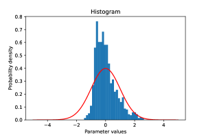
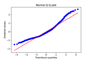
Figure 1: Histogram and density function of a standard normal distribution (left) and Normal Q-Q plot (right) through $1000$ experiments in the case $H=0.75,\theta=1.0,\varepsilon=1.0,T=1.0,n=100$

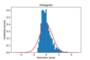
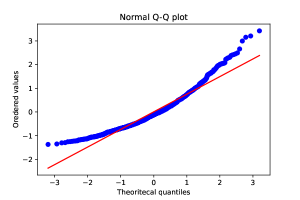
Figure 2: Histogram and density function of a standard normal distribution (left) and Normal Q-Q plot (right) through $1000$ experiments in the case $H=0.75,\theta=1.0,\varepsilon=1.0,T=1.0,n=500$

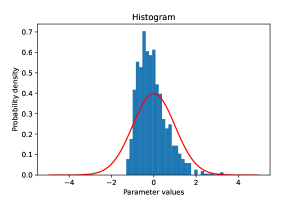
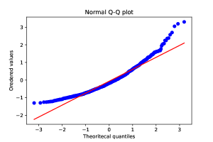
Figure 3: Histogram and density function of a standard normal distribution (left) and Normal Q-Q plot (right) through $1000$ experiments in the case $H=0.75,\theta=1.0,\varepsilon=1.0,T=1.0,n=1000$

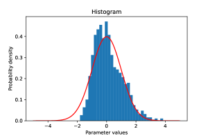
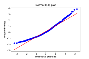
Figure 4: Histogram and density function of a standard normal distribution (left) and Normal Q-Q plot (right) through $1000$ experiments in the case $H=0.75,\theta=1.0,\varepsilon=0.5,T=1.0,n=100$

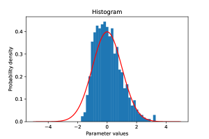
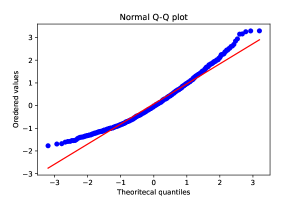
Figure 5: Histogram and density function of a standard normal distribution (left) and Normal Q-Q plot (right) through $1000$ experiments in the case $H=0.75,\theta=1.0,\varepsilon=0.5,T=1.0,n=500$

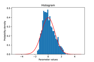
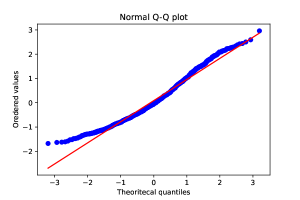
Figure 6: Histogram and density function of a standard normal distribution (left) and Normal Q-Q plot (right) through $1000$ experiments in the case $H=0.75,\theta=1.0,\varepsilon=0.5,T=1.0,n=1000$

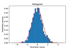
Figure 7: Histogram and density function of a standard normal distribution (left) and Normal Q-Q plot (right) through $1000$ experiments in the case $H=0.75,\theta=1.0,\varepsilon=0.1,T=1.0,n=100$

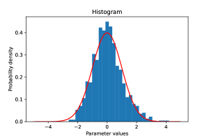
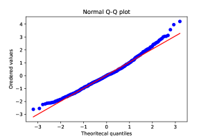
Figure 8: Histogram and density function of a standard normal distribution (left) and Normal Q-Q plot (right) through $1000$ experiments in the case $H=0.75,\theta=1.0,\varepsilon=0.1,T=1.0,n=500$

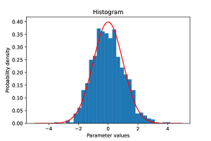
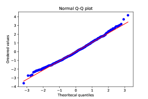
Figure 9: Histogram and density function of a standard normal distribution (left) and Normal Q-Q plot (right) through $1000$ experiments in the case $H=0.75,\theta=1.0,\varepsilon=0.1,T=1.0,n=1000$

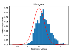
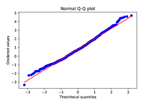
Figure 10: Histogram and density function of a standard normal distribution (left) and Normal Q-Q plot (right) through $1000$ experiments in the case $H=0.25,\theta=1.0,\varepsilon=0.1,T=1.0,n=100$

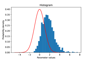
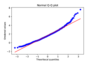
Figure 11: Histogram and density function of a standard normal distribution (left) and Normal Q-Q plot (right) through $1000$ experiments in the case $H=0.25,\theta=1.0,\varepsilon=0.1,T=1.0,n=500$

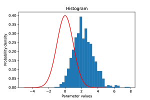
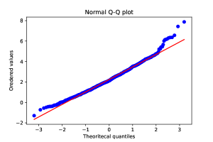
Figure 12: Histogram and density function of a standard normal distribution (left) and Normal Q-Q plot (right) through $1000$ experiments in the case $H=0.25,\theta=1.0,\varepsilon=0.1,T=1.0,n=1000$

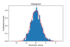
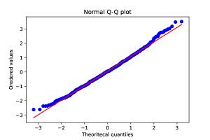
Figure 13: Histogram and density function of a standard normal distribution (left) and Normal Q-Q plot (right) through $1000$ experiments in the case $H=0.25,\theta=1.0,\varepsilon=0.01,T=1.0,n=100$

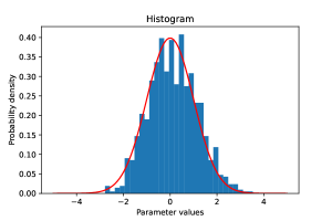
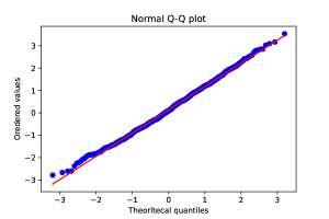
Figure 14: Histogram and density function of a standard normal distribution (left) and Normal Q-Q plot (right) through $1000$ experiments in the case $H=0.25,\theta=1.0,\varepsilon=0.01,T=1.0,n=500$

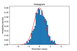
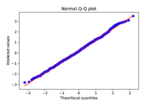
Figure 15: Histogram and density function of a standard normal distribution (left) and Normal Q-Q plot (right) through $1000$ experiments in the case $H=0.25,\theta=1.0,\varepsilon=0.01,T=1.0,n=1000$

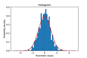
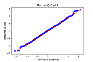
Figure 16: Histogram and density function of a standard normal distribution (left) and Normal Q-Q plot (right) through $1000$ experiments in the case $H=0.25,\theta=1.0,\varepsilon=0.005,T=1.0,n=100$

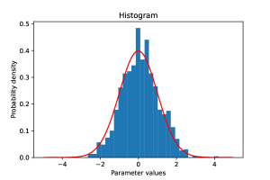
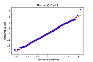
Figure 17: Histogram and density function of a standard normal distribution (left) and Normal Q-Q plot (right) through $1000$ experiments in the case $H=0.25,\theta=1.0,\varepsilon=0.005,T=1.0,n=500$

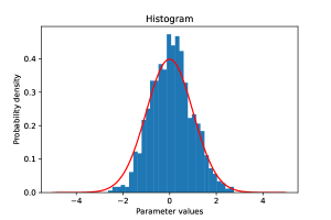
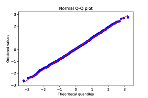
Figure 18: Histogram and density function of a standard normal distribution (left) and Normal Q-Q plot (right) through $1000$ experiments in the case $H=0.25,\theta=1.0,\varepsilon=0.005,T=1.0,n=1000$

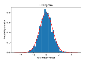
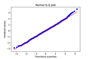
Figure 19: Histogram and density function of a standard normal distribution (left) and Normal Q-Q plot (right) through $1000$ experiments in the case $H=0.25,\theta=1.0,\varepsilon=0.001,T=1.0,n=100$

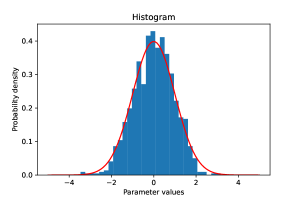
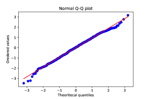
Figure 20: Histogram and density function of a standard normal distribution (left) and Normal Q-Q plot (right) through $1000$ experiments in the case $H=0.25,\theta=1.0,\varepsilon=0.001,T=1.0,n=500$

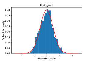
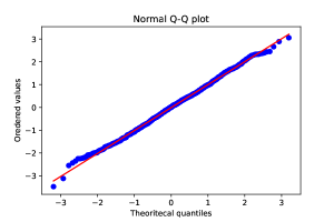
Figure 21: Histogram and density function of a standard normal distribution (left) and Normal Q-Q plot (right) through $1000$ experiments in the case $H=0.25,\theta=1.0,\varepsilon=0.001,T=1.0,n=1000$

From Table 1-2, we can observe the strong consistency results in Theorem 1 hold true when $\varepsilon\rightarrow 0,n\rightarrow\infty$. In addition, we can see that asymptotic normality in Theorem 2 hold from Figure 1-9 and Figure 13-21. When $H=0.25$ and $\varepsilon=0.1$ , the convergence order assumptions of Theorem 2 is not satisfied for $n=100,500,1000$, so we can observe that asymptotic normality does not hold, as shown in Figure 10-12.

References

- [1] Biagini, F.; Hu, Y.; Øksendal, B. and Zhang, T. (2008). Stochastic calculus for fractional Brownian motion and applications. Probability and its Applications. Springer-Verlag London, Ltd., London.
- [2] Brouste, A. and Kleptsyna, M. (2010). Asymptotic properties of MLE for partially observed fractional diffusion system. Stat. Inference Stoch. Process. 13(1), 1-13.
- [3] Chiba, K. (2020). An M-estimator for stochastic differential equations driven by fractional Brownian motion with small Hurst parameter. Stat. Inference Stoch. Process. 23, no. 2, 319-353.
- [4] Frydman, R. (1980). A proof of the consistency of maximum likelihood estimators of nonlinear regression models with autocorrelated errors. Econometrica 48, no. 4, 853-860.
- [5] Hu, Y.; Nualart, D. and Zhou, H. (2017). Parameter estimation for fractional Ornstein-Uhlenbeck processes of general Hurst parameter. Stat Inference Stoch Process, 22, 1-32.
- [6] Hu Y.; Nualart, D. and Zhou, H. (2019). Drift parameter estimation for nonlinear stochastic differential equations driven by fractional Brownian motion. Stochastics 91, 1-25.
- [7] Kasonga, R. A. (1998). The consistency of a nonlinear least-squares estimator from diffusion processes. Stochastic Process. Appl. 30, no. 2, 263-275.
- [8] Kleptsyn, M. and Le Breton, A. (2002). Statistical analysis of the fractional Ornstein-Uhlenbeck type process. Stat. Inference Stoch. Process. 5(3), 229-248.
- [9] Kubilius, K.; Mishura, Y. and Ralchenko, K. (2017). Parameter estimation in fractional diffusion models. Bocconi & Springer Series, 8. Bocconi and Springer series. Springer, Berlin
- [10] Kutoyants, U. A. (1984). Parameter Estimation for Stochastic Processes, Heldermann, Berlin.
- [11] Kutoyants, U. A. (1994). Identification of Dynamical Systems with Small Noise. Kluwer, Dordrecht.
- [12] Lohvinenko, S. and Ralchenko, K. (2017). Maximum likelihood estimation in the fractional Vasicek model. Lith J Stat, 56 (1), 77-87.
- [13] Long, H.; Shimizu, Y. and Sun, W. (2013). Least-squares estimators for discretely observed stochastic processes driven by small Lévy noises. J. Multivariate Anal. 116, 422-439.
- [14] Nakajima, S. and Shimizu, Y. (2021). Asymptotic normality of least squares estimators to stochastic differential equations driven by fractional Brownian motions. Preprint arXiv:2112.12333.
- [15] Nakajima, S. and Shimizu, Y. (2022). Parameter estimation of stochastic differential equation driven by small fractional noise. Preprint arXiv:2201.00372.
- [16] Nualart, D. (1995). Malliavin calculus and related topics. (Probability and its Applications). Berlin Heidelberg New York Springer.
- [17] Neuenkirch, A. and Nourdin, I. (2007). The exact rate of convergence of some approximation schemes associated with SDEs driven by a fractional Brownian motion. J. Theoret. Probab. 20, no. 4, 871-899.
- [18] Neuenkirch, A. and Tindel, S. (2014). A least square-type procedure for parameter estimation in stochastic differential equations with additive fractional noise. Stat. Inference Stoch. Process. 17(1), 99-120.
- [19] Prakasa Rao, B. L. S. (1999). Statistical inference for diffusion type processes. Kendall’s Library of Statistics, 8. Edward Arnold, London; Oxford University Press, New York.
- [20] Rao, B. P. (2011). Statistical inference for fractional diffusion processes. Wile, Berlin.
- [21] Tanaka, K.; Xiao, W. and Yu, J. (2019). Maximum likelihood estimation for the fractional Vasicek model. SMU Econ Stat Work Paper Series, 2019(8).
- [22] Tudor, C. A. and Viens, F. G. (2007). Statistical aspects of the fractional stochastic calculus. Ann Stat. 35 (3),1183-1212.
- [23] Uchida, M. and Yoshida, N. (2004). Information criteria for small diffusions via the theory of Malliavin-Watanabe, Stat. Inference Stoch. Process. 7, 35-67.
- [24] Yoshida, N. (1992). Asymptotic expansion of maximum likelihood estimators for small diffusions via the theory of Malliavin-Watanabe. Probab. Theory Relat. Fields. 92, 275-3-1.
- [25] Yoshida, N. (2003). Conditional expansions and their applications. Stochastic Process. Appl. 107. 53-81.
- [26] Young, L.C. (1936). An inequality of Hölder type, connected with Stieltjes integration, Acta Math., 67, 251-282.
- [27] Zähle, M. (2005). Stochastic differential equations with fractal noise. Math. Nachr. 278(9), 1097-1106.