Cosmic rays in molecular clouds
probed by H₂ rovibrational lines

Abstract

Context. Low-energy cosmic rays (¡ TeV) play a fundamental role in the chemical and dynamical evolution of molecular clouds, as they control the ionisation, dissociation, and excitation of H₂. Their characterisation is therefore important both for the interpretation of observations and for the development of theoretical models. However, the methods used so far for estimating the cosmic-ray ionisation rate in molecular clouds have several limitations due to uncertainties in the adopted chemical networks.

Aims. We refine and extend the method proposed by Bialy (2020) to estimate the cosmic-ray ionisation rate in molecular clouds by observing rovibrational transitions of H₂ at near-infrared wavelengths, which are mainly excited by secondary cosmic-ray electrons.

Methods. Combining models of interstellar cosmic-ray propagation and attenuation in molecular clouds with the rigorous calculation of the expected secondary electron spectrum and updated H₂ excitation cross sections by electron collisions, we derive the intensity of the four H₂ rovibrational transitions observable in dense, cold gas: $(1-0){\rm O}(2)$, $(1-0){\rm Q}(2)$, $(1-0){\rm S}(0)$, and $(1-0){\rm O}(4)$.

Results. The proposed method allows the estimation of the cosmic-ray ionisation rate for a given observed line intensity and H₂ column density. We are also able to deduce the shape of the low-energy cosmic-ray proton spectrum impinging upon the molecular cloud. We also present a look-up plot and a web-based application that can be used to constrain the low-energy spectral slope of the interstellar cosmic-ray proton spectrum. We finally comment on the capability of the James Webb Space Telescope to detect these near-infrared H₂ lines, making it possible to derive for the first time spatial variation of the cosmic-ray ionisation rate in dense gas. Besides the implications for the interpretation of the chemical-dynamic evolution of a molecular cloud, it will finally be possible to test competing models of cosmic-ray propagation and attenuation in the interstellar medium, as well as compare cosmic-ray spectra in different Galactic regions.

1 Introduction

Cosmic rays (CRs) at sub-TeV energies play an important role in the energetics and the physico-chemical evolution of star-forming regions. Their energy density, of the order of 1 eV cm^-3, is comparable to that of the Galactic magnetic field, of the cosmic microwave background, and of the visible starlight (Ferrière, 2001). By ionising molecular hydrogen, the main constituent of molecular clouds, CRs trigger a cascade of chemical reactions leading to the formation of increasingly complex molecules, up to prebiotic species. Furthermore, by determining the ionisation fraction, they regulate the degree of coupling between gas and magnetic field and thus affects the collapse timescale of a cloud (see Padovani et al., 2020, for a review).

CR particles include electrons, protons and heavier nuclei. The electron component is revealed by Galactic synchrotron emission, that depends on the strength of the interstellar magnetic field (e.g. Ginzburg & Syrovatskii, 1965; Orlando, 2018; Padovani & Galli, 2018; Padovani et al., 2021a). Direct constraints on the spectrum of CR electrons can be obtained from synchrotron observations only if the magnetic field strength can be independently estimated by other methods, e.g. by modelling the polarised dust thermal emission (Alves et al., 2018; Beltrán et al., 2019; Sanhueza et al., 2021). The proton component of CRs above $\simeq 1$ GeV can be constrained through observations of local $\gamma$-ray emissivity due to pion decay (Casandjian, 2015; Strong & Fermi-LAT Collaboration, 2015; Orlando, 2018). However, the results depend on the assumed CR propagation and solar modulation models (see also Tibaldo et al., 2021, for a review). At lower energies, between about 3 and 300 MeV, the local interstellar CR spectrum is constrained by in situ measurements obtained by the two Voyager spacecrafts (Cummings et al., 2016; Stone et al., 2019). Still, the magnetic field direction measured by the Voyager probes did not show the change expected if they were beyond the influence of solar modulation (Gloeckler & Fisk, 2015). Consequently, there is a substantial uncertainty about the low-energy CR spectrum. In addition, fluctuations in the CR spectrum across the Galaxy could be present, due to the discrete nature of the CR sources (Phan et al., 2021).

Several observational techniques provide an estimate of the spectrum of low-energy CRs in interstellar clouds by determining the ionisation rate, $\zeta_{\rm ion}$, i.e. the number of ionisations of hydrogen atoms or molecules per unit time. In the diffuse regions of molecular clouds, the CR ionisation rate can be inferred from absorption line studies of H${}_{3}^{+}$ (Oka, 2006; Indriolo & McCall, 2013), OH⁺, H₂O⁺ (see e.g. Neufeld et al., 2010), and ArH⁺ (Neufeld & Wolfire, 2017; Bialy et al., 2019). Even though the method based on H${}_{3}^{+}$ absorption lines is commonly considered as one of the most reliable, thanks to a particularly simple chemistry controlling the H${}_{3}^{+}$ abundance (Oka, 2006), there is a number of observational and model limitations that restrict the choice of possible target clouds and may introduce significant uncertainties in estimating the value of $\zeta_{\rm ion}$. These limitations include the need of having an early-type star in the background, in order to evaluate H${}_{3}^{+}$ and H₂ column densities along the same line of sight (Indriolo & McCall, 2012). Furthermore, the value of $\zeta_{\rm ion}$ obtained from this method is proportional to the gas volume density and therefore is affected by uncertainties in estimating the latter in the probed cloud regions (Jenkins & Tripp, 2001; Sonnentrucker et al., 2007; Jenkins & Tripp, 2011; Goldsmith, 2013). Finally, possible strong variations in the H${}_{3}^{+}$ abundance along the line of sight, caused by uncertainties in the local ionisation fraction, which depends on details of interstellar UV attenuation in the cloud (see Neufeld & Wolfire, 2017), may also significantly affect the resulting value of $\zeta_{\rm ion}$.

In denser regions other tracers of $\zeta_{\rm ion}$ are used, such as HCO⁺, DCO⁺, and CO in low-mass dense cores (Caselli et al., 1998), HCO⁺, N₂H⁺, HC₃N, HC₅N, and c-C₃H₂ in protostellar clusters (Ceccarelli et al., 2014; Fontani et al., 2017; Favre et al., 2018), and more recently H₂D⁺ and other H${}_{3}^{+}$ isotopologues in high-mass star-forming regions (Bovino et al., 2020; Sabatini et al., 2020). The downside is that the chemistry in these high-density regions is much more complex than in diffuse clouds, requiring comprehensive and updated reaction networks. In this case, the main source of uncertainty comes from the formation and destruction rates of some species, which are not well established, as well as from the poorly constrained amount of carbon and oxygen depletion on dust grains.

We note that the picture is further complicated by the effects of magnetic fields. If field lines are tangled and/or the magnetic field strength is not constant, as expected in turbulent star-forming regions, CRs can be attenuated more effectively, further reducing $\zeta_{\rm ion}$ (Padovani & Galli, 2011; Padovani et al., 2013; Silsbee et al., 2018).

Recently, Bialy (2020) developed a new method to estimate the CR ionisation rate from infrared observations of rovibrational line emissions of H₂. This approach reduces the degree of uncertainty on the determination of $\zeta_{\rm ion}$ with respect to the methods listed above, as neither chemical networks nor abundances of other secondary species are involved. These H₂ rovibrational transitions are collisionally excited by secondary electrons produced during the propagation of primary CRs. In dense molecular clouds most of the H₂ is in the para form (Bovino et al., 2017; Lupi et al., 2021). As we show in Sect. 4, CRs and UV photons determine the rovibrational excitation from the $(v,J)=(0,0)$ level to the $(v,J)=(1,0)$ and $(1,2)$ levels. The subsequent radiative decay to the $v=0$ level results in the emission of infrared photons at wavelengths of 2–$3\leavevmode\nobreak\ \mu$m (see Table 1). These photons can be detected by devices such as X-shooter, mounted on the Very Large Telescope (VLT), the Magellan Infrared Spectrograph (MMIRS), mounted on the Multiple Mirror Telescope (MMT), see Bialy et al. (2021), and by forthcoming facilities such as the Near Infrared Spectrograph (NIRSpec) on board the James Webb Space Telescope (JWST). We only consider even-$J$ transitions with $\Delta J=0,\pm 2$ (see third column of Table 1) since $|\Delta J|>2$ transitions have negligible probability (Itikawa & Mason, 2005). Besides, odd-$J$ transitions are not frequent in dense molecular clouds (Flower & Watt, 1984) as they involve ortho-to-para conversion due to reactive collisions with protons. We also checked that the contribution to the excitation of the $(v,J)=(1,0)$ and $(1,2)$ levels by higher vibrational levels is negligible. For example, the contribution from the $v=2$ level to observed line intensities is less than about 5%.

In this article we refine and extend the method developed by Bialy (2020), taking into account recent advances on the calculation of the secondary electron spectrum (Ivlev et al., 2021) and updated, accurate H₂ rovibrational cross sections calculated using the molecular convergent close-coupling (MCCC) method. Thanks to these recent results, we can relax approximations previously made, like, e.g., a secondary electron spectrum with an average energy of about 30 eV (Cravens & Dalgarno, 1978) and a constant ratio of CR excitation and ionisation rates independent of the H₂ column density (Gredel & Dalgarno, 1995; Bialy, 2020). In addition, we adopt here the local CR spectrum as the main parameter of our model. Given the strong dependence on energy of the cross sections of the processes involved, a spectrum-dependent analysis provides a better parametrisation of the results than a spectrum-integrated quantity like $\zeta_{\rm ion}$, as assumed by Bialy (2020). Assuming a free-streaming regime of CR propagation, we show that, provided the H₂ column density is known, the intensity of these infrared H₂ lines can constrain both the CR ionisation rate and the spectral energy slope of the interstellar CR proton spectrum at low energies, This considerably reduces the degree of uncertainty compared to other methods.

This paper is organised as follows. In Sect. 2 we review the state-of-the-art calculations of the cross sections, and compute an updated energy loss function for electrons in H₂, which we use to derive the secondary electron spectrum. In Sect. 3 we calculate the CR excitation rates of H₂ and compare them with the CR ionisation rates. In Sect. 5 we apply the above results to compute the expected observed brightness of the H₂ rovibrational transitions, providing a look-up plot that can be used for a direct estimate of the CR ionisation rate and of the low-energy spectral slope of CR protons. We also describe the capabilities of JWST in detecting the infrared emission of these H₂ lines. In Sect. 6 we summarise our main findings.

2 Derivation of the secondary electron spectrum

The brightest H₂ rovibrational transitions at near-infrared wavelengths, between 2.22 and 3 $\mu$m, are listed in Table 1.

Table 1: H₂ rovibrational transitions.

Transition	Upper level $(v,J)$	Lower level $(v^{\prime},J^{\prime})$	$\lambda$ [$\mu$m]
$(1-0){\rm O}(2)$	(1,0)	(0,2)	2.63
$(1-0){\rm Q}(2)$	(1,2)	(0,2)	2.41
$(1-0){\rm S}(0)$	(1,2)	(0,0)	2.22
$(1-0){\rm O}(4)$	(1,2)	(0,4)	3.00

Their upper levels, $(v,J)=(1,0)$ and $(1,2)$, can be populated very effectively by CR excitation and, to a lesser extent, by UV or H₂ formation pumping, respectively (see Bialy 2020 and Sect. 5). CR excitation is dominated by low-energy secondary electrons produced during the propagation of interstellar CRs, while primary CRs (both protons and electrons) provide a negligible contribution to the excitation rate (see Sect. 3). The rovibrational cross sections of the transitions of interest, $(v,J)=(0,0)\rightarrow(1,0)$ and $(0,0)\rightarrow(1,2)$ (see second column of Table 1) have a maximum around 3–4 eV with a threshold at $\sim 0.5$ eV. Therefore, in order to calculate the excitation rates, the secondary electron spectrum down to $\sim 0.5$ eV needs to be accurately determined.

Ivlev et al. (2021) developed a rigorous theory for calculating the secondary electron spectrum as a function of the primary CR proton spectrum and column density, and applied this method to determine the secondary spectrum above the H₂ ionisation threshold ($I=15.44$ eV). In this paper, we extend the calculations of Ivlev et al. (2021) to lower energies, down to 0.5 eV, and also include secondary electrons produced by primary CR electrons. To this goal, the balance equation accounting for all population and depopulation processes of a given energy bin of secondary electrons must also include processes occurring at energies $E<I$, such as momentum transfer, rotational excitation $J=0\rightarrow 2$ and vibrational excitations $v=0\rightarrow 1$ and $v=0\rightarrow 2$ (see Sect. 4.4 in Ivlev et al., 2021, for details). In our previous works (e.g. Padovani et al., 2009, 2018b; Ivlev et al., 2021), we made use of the cross sections summarised by Dalgarno et al. (1999) and the analytical fits of Janev et al. (2003). Recently, a number of theoretical and experimental studies on the H₂ electronic excitation have been published, and in Sect. 2.1 we comment on the differences with previous studies.

2.1 Cross sections

In Fig. 1 we compare available experimental data and earlier theoretical calculations of the main excitation cross sections with the most recent computations adopted in this work (shown by thick solid lines). For the electronic excitation cross sections we use the most recent and accurate results produced using the MCCC method (Scarlett et al., 2021a). These cross sections have already been employing in plasma modelling (Wünderlich et al., 2021), leading to much better agreement with measurements compared to the previously-used datasets of Miles et al. (1972) and Janev et al. (2003). The MCCC results are summarised by Scarlett et al. (2021a) and are accessible through a web database.

For many transitions, the MCCC method results were found to be in disagreement with previously recommended excitation cross sections (e.g. Yoon et al., 2008). The most striking difference is for the $X\,^{1}\Sigma_{g}^{+}\rightarrow b\,^{3}\Sigma_{u}^{+}$ transition, where peak values are twice lower than what recommended (Scarlett et al., 2017; Zammit et al., 2017), with important consequences on the energy loss function (see Sect. 2.2). On the other hand, recent experimental results are in perfect agreement with the MCCC calculations (Zawadzki et al., 2018a, b).

As for the $X\,^{1}\Sigma_{g}^{+}\rightarrow B\,^{1}\Sigma_{u}^{+}$ and $X\,^{1}\Sigma_{g}^{+}\rightarrow C\,^{1}\Pi_{u}$ cross sections, there are no recent measurements in the energy region close to the cross section peak. We adopt the MCCC calculations because the method is essentially without approximation, aside from the adiabatic-nuclei approximation which is of no consequence at the energies of interest, where there is disagreement with older experiments. Since for elastic, grand-total, ionisation, and the $X\,^{1}\Sigma_{g}^{+}\rightarrow b\,^{3}\Sigma_{u}^{+}$ cross sections the MCCC results are in near-perfect agreement with experiment, we adopt the $X\,^{1}\Sigma_{g}^{+}\rightarrow B\,^{1}\Sigma_{u}^{+}$ and $X\,^{1}\Sigma_{g}^{+}\rightarrow C\,^{1}\Pi_{u}$ cross sections from the MCCC method as well. However, close to the energy peak of the singlet cross sections the dominant electron loss process is ionisation (see Fig. 2), therefore this difference has no consequences for our purposes.

Recently, Scarlett et al. (2021b) applied the MCCC method to calculate rovibrationally-resolved cross sections for the $X\,^{1}\Sigma_{g}^{+}\rightarrow d\,^{3}\Pi_{u}$ transition, in order to study the polarisation of Fulcher-$\alpha$ fluorescence. Here, we apply the same method to calculate cross sections for the rovibrational transitions listed in Table 1.

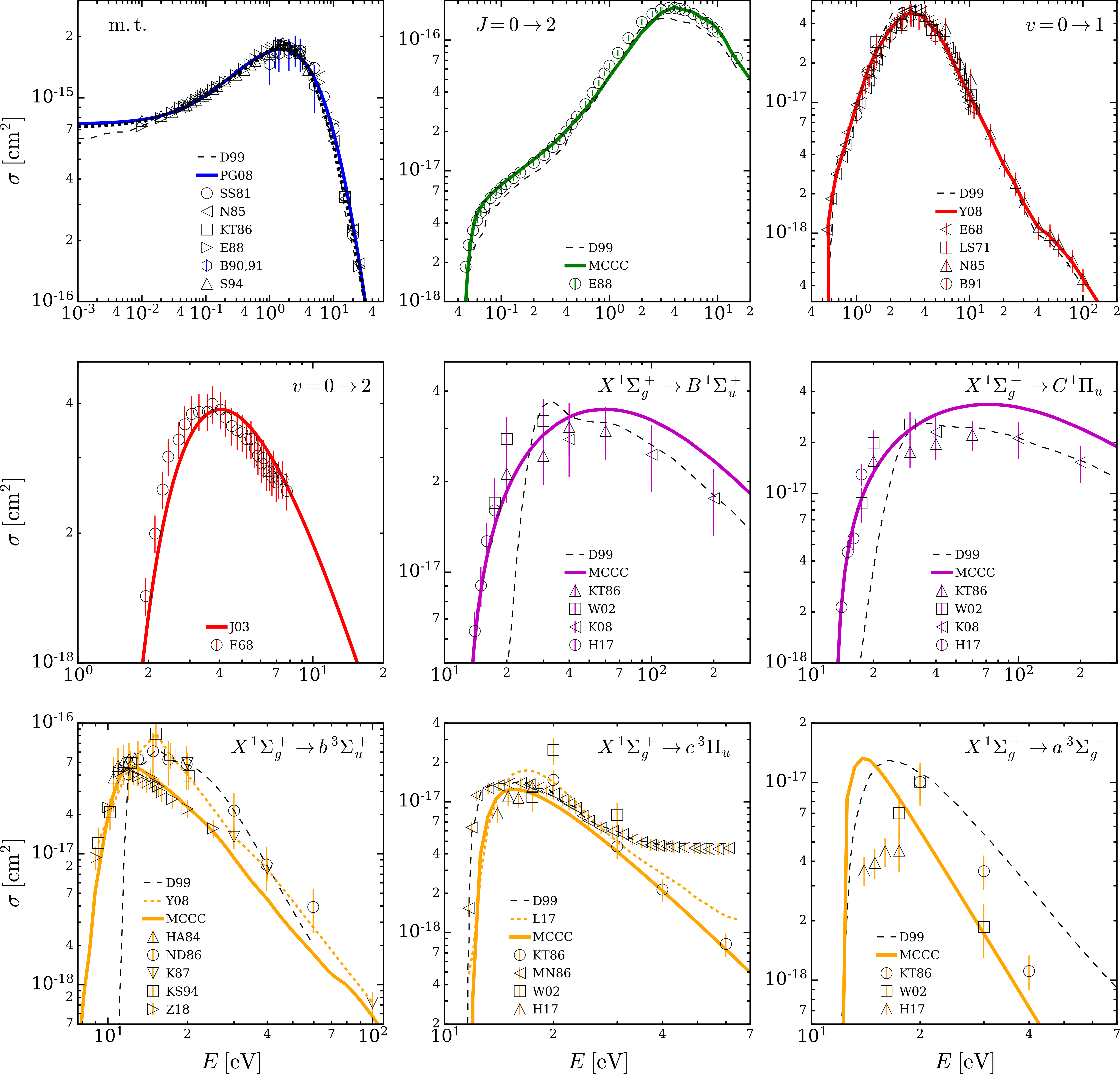
Figure 1: Theoretical and experimental cross sections for electrons colliding with H₂. The cross sections used for the calculation of the energy loss function are displayed as thick lines, those adopted by Dalgarno et al. (1999) (D99) by black dashed lines. From left to right and from top to bottom: momentum transfer cross section (“m.t.”) - solid thick blue line (Pinto & Galli, 2008, PG08), circles (Shyn & Sharp, 1981, SS81), left-pointing triangles (Nishimura et al., 1985, N85), squares (Khakoo & Trajmar, 1986, KT86), right-pointing triangles (England et al., 1988, E88), hexagons (Brunger et al., 1990, 1991, B90,91), up-pointing triangles (Schmidt et al., 1994, S94); rotational transition $J=0\rightarrow 2$ - solid thick green line (present MCCC calculations), circles (England et al., 1988, E88); vibrational transition $v=0\rightarrow 1$ - solid thick red line (Yoon et al., 2008, Y08), left-pointing triangles (Ehrhardt et al., 1968, E68), squares (Linder & Schmidt, 1971, LS71), up-pointing triangles (Nishimura et al., 1985, N85), circles (Brunger et al., 1991, B91); vibrational transition $v=0\rightarrow 2$ - solid thick red line (Janev et al., 2003, J03), circles (Ehrhardt et al., 1968, E68); $X\,^{1}\Sigma_{g}^{+}\rightarrow B\,^{1}\Sigma_{u}^{+}$ and $X\,^{1}\Sigma_{g}^{+}\rightarrow C\,^{1}\Pi_{u}$ singlet transitions - solid thick magenta line (Scarlett et al., 2021a, MCCC), up-pointing triangles (Khakoo & Trajmar, 1986, KT86), squares (Wrkich et al., 2002, W02), left-pointing triangles (Kato et al., 2008, K08), circles (Hargreaves et al., 2017, H17); $X\,^{1}\Sigma_{g}^{+}\rightarrow b\,^{3}\Sigma_{u}^{+}$ triplet transition - dotted orange line (Yoon et al., 2008, Y08), solid thick orange line (Scarlett et al., 2021a, MCCC), up-pointing triangles (Hall & Andric, 1984, HA84), circles (Nishimura & Danjo, 1986, ND86), down-pointing triangles (Khakoo et al., 1987, K87), squares (Khakoo & Segura, 1994, KS94), right-pointing triangles (Zawadzki et al., 2018a, Z18); $X\,^{1}\Sigma_{g}^{+}\rightarrow c\,^{3}\Pi_{u}$ triplet transition - dotted orange line (Liu et al., 2017, L17), solid thick orange line (Scarlett et al., 2021a, MCCC), circles (Khakoo & Trajmar, 1986, KT86), left-pointing triangles (Mason & Newell, 1986, MN86), squares (Wrkich et al., 2002, W02), up-pointing triangles (Hargreaves et al., 2017, H17); $X\,^{1}\Sigma_{g}^{+}\rightarrow a\,^{3}\Sigma_{g}^{+}$ triplet transition - solid thick orange line (Scarlett et al., 2021a, MCCC), circles (Khakoo & Trajmar, 1986, KT86), squares (Wrkich et al., 2002, W02), up-pointing triangles (Hargreaves et al., 2017, H17).

2.2 Electron energy loss function

The quantity that controls the energy degradation of a particle propagating through a medium is the so-called energy loss function. For electrons colliding with H₂, it is described by

$$L_{e}(E) = \frac{2m_{e}}{m_{\rm H_{2}}}\sigma_{\rm m.t.}(E)E+\sum_{j}\sigma_{{\rm exc},j}(E)E_{{\rm thr},j}+$$

$$\int_{0}^{(E-I)/2}\frac{{\rm d}\sigma_{\rm ion}(E,\varepsilon)}{{\rm d}\varepsilon}(I+\varepsilon){\rm d}\varepsilon+$$

$$\int_{0}^{E}\frac{{\rm d}\sigma_{\rm br}(E,E_{\gamma})}{{\rm d}E_{\gamma}}E_{\gamma}{\rm d}E_{\gamma}+KE^{2}\,.$$

Terms on the right-hand side represent the contributions of momentum transfer, rotational, vibrational, and electronic excitation, ionisation, and bremsstrahlung. In addition, the last term on the right-hand side represents synchrotron losses that only depend on the strength of the magnetic field in the cloud. Here, $m_{e}$ and $m_{\rm H_{2}}$ are the electron and H₂ mass, respectively, $\sigma_{\rm m.t.}$ and $\sigma_{{\rm exc},j}$ are the cross section of momentum transfer and excitation of state $j$ summarised in Fig. 1, $E_{{\rm thr},j}$ is the corresponding excitation threshold energy, ${\rm d}\sigma_{\rm ion}/{\rm d}\varepsilon$ is the differential ionisation cross section (Kim et al., 2000), where $\varepsilon$ is the secondary electron energy, and ${\rm d}\sigma_{\rm br}/{\rm d}E_{\gamma}$ is the differential bremsstrahlung cross section (Blumenthal & Gould, 1970), where $E_{\gamma}$ is the energy of the emitted photon. Finally, $KE^{2}$ represents synchrotron losses with $K=5\times 10^{-38}$ eV cm² and $E$ in eV (Schlickeiser, 2002). For typical temperatures ($T\simeq 10$ K) and ionisation fractions ($x_{e}<10^{-7}$), Coulomb losses are negligible in the energy range of interest (Swartz et al., 1971). For clarity, we show the loss functions for the electronic excitation summed over all the triplet states ($b\,^{3}\Sigma_{u}^{+}$, $a\,^{3}\Sigma_{g}^{+}$, $c\,^{3}\Pi_{u}$, $e\,^{3}\Sigma_{u}^{+}$, $h\,^{3}\Sigma_{g}^{+}$, $d\,^{3}\Pi_{u}$, $g\,^{3}\Sigma_{g}^{+}$, $i\,^{3}\Pi_{g}$, and $j\,^{3}\Delta_{g}$) and the singlet states ($B\,^{1}\Sigma_{u}^{+}$, $C\,^{1}\Pi_{u}$, $EF\,^{1}\Sigma_{g}^{+}$, $B^{\prime}\,{}^{1}\Sigma_{u}^{+}$, $GK\,^{1}\Sigma_{g}^{+}$, $I\,^{1}\Pi_{g}$, $J\,^{1}\Delta_{g}$, $D\,^{1}\Pi_{u}$, and $H\,^{1}\Sigma_{g}^{+}$).

The resulting energy loss function, $L_{e}(E)$, shown in Fig. 2, differs in two energy ranges from the one adopted in our previous works (e.g. Padovani et al., 2009, 2018b), which was based on the cross sections by Dalgarno et al. (1999) and data from the National Institute of Standards and Technology database. We note that, while Dalgarno et al. (1999) assume an ortho-to-para ratio of 3:1, we assume that molecular hydrogen is uniquely in the form of para-H₂ (see Sect. 1). The new loss function is a factor of $\simeq 3$ larger between 0.05 and 0.1 eV due to the different assumption on temperature and ortho-to-para ratio, and is up to 20 times larger in the range $7-12$ eV, mainly due to the updated $X\,^{1}\Sigma_{g}^{+}\rightarrow b\,^{3}\Sigma_{u}^{+}$ excitation cross section. For our purposes, the latter difference is especially important for the derivation of the spectrum of secondaries below the H₂ ionisation threshold.

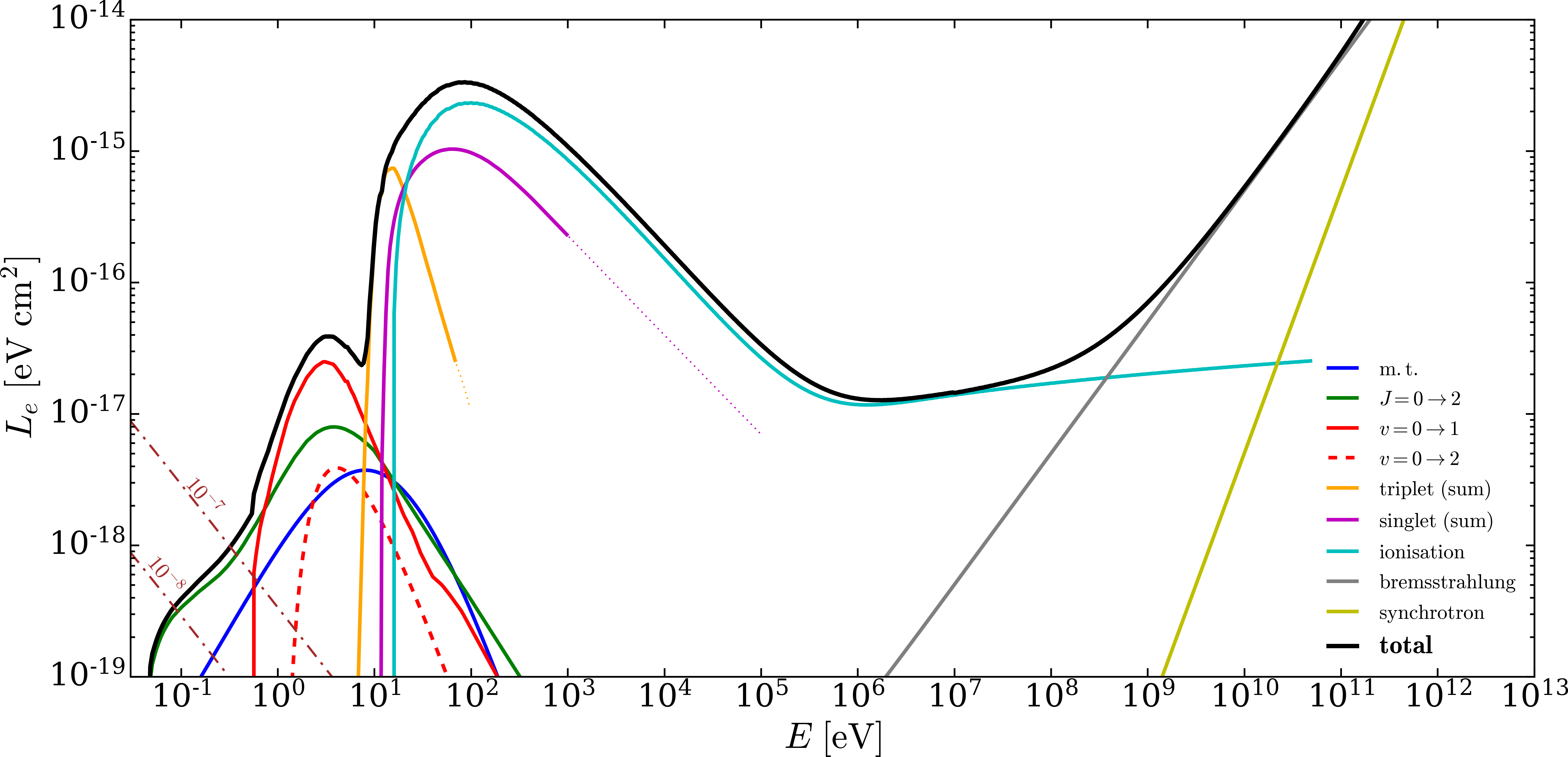
Figure 2: Energy loss function for electrons colliding with H₂ including the contribution of synchrotron losses (solid black line). Coloured lines show the different components (the following references refer to the papers from which the relative cross sections have been adopted). Momentum transfer (“m.t.”, solid blue; Pinto & Galli 2008); rotational transition $J=0\rightarrow 2$ (solid green line; England et al. 1988); vibrational transitions $v=0\rightarrow 1$ (solid red line; Yoon et al. 2008) and $v=0\rightarrow 2$ (dashed red line; Janev et al. 2003); electronic transitions summed over all the triplet and singlet states (solid orange and magenta lines, respectively; Scarlett et al. 2021a); ionisation (solid cyan line; Kim et al. 2000); bremsstrahlung (solid grey line; Blumenthal & Gould 1970; Padovani et al. 2018b); synchrotron (solid yellow line; Schlickeiser 2002; Padovani et al. 2018b). Dash-dotted brown lines show the Coulomb losses at 10 K for ionisation fractions, $x_{e}$, equal to $10^{-7}$ and $10^{-8}$ (Swartz et al., 1971).

2.3 Spectrum of secondary electrons

We extend the solution of the balance equation, Eq. (27) in Ivlev et al. (2021), down to $0.5$ eV to compute the secondary electron spectrum at various H₂ column densities. We also checked the effect of a change in the composition of the medium, including a fraction of He equal to $\simeq 20\%$ (see Table A.1 in Padovani et al., 2018b). However, the additional contribution to the spectrum of secondaries is on average smaller than 3% and we therefore disregard it. For completeness, in Appendix A, we show the energy loss function for electrons colliding with He atoms and the cross sections adopted for its derivation.

For the calculation of the secondary electron spectrum, we assume the analytic form for the interstellar CR spectrum from Padovani et al. (2018b)

$$j_{k}^{\rm IS}(E)=C\frac{E^{\alpha}}{(E+E_{0})^{\beta}}\leavevmode\nobreak\ {\rm eV^{-1}\leavevmode\nobreak\ s^{-1}\leavevmode\nobreak\ cm^{-2}\leavevmode\nobreak\ sr^{-1}}\,,$$ (2)

where $k=e,p$. The adopted values of the parameters $C$, $E_{0}$, $\alpha$, and $\beta$ are listed in Table 2. For protons we assume two possible low-energy spectral shapes: one, with $\alpha=0.1$, reproduces the most recent Voyager 1 and 2 data (Cummings et al., 2016; Stone et al., 2019), labelled as ‘low’ spectrum $\mathscr{L}$; the other, with $\alpha=-0.8$, better reproduces the average trend of the CR ionisation rate estimated from observations in diffuse clouds (Shaw et al., 2008; Neufeld et al., 2010; Indriolo & McCall, 2012; Neufeld & Wolfire, 2017, see also Appendix C) and it is labelled as ‘high’ spectrum $\mathscr{H}$. For the sake of clarity, in this section we consider only these two values of $\alpha$ for protons, but in the following sections we allow for the whole range of $\alpha$ values, from $-1.2$ to $0.1$ (see left panel of Fig. 3). As we show in the following sections, most of the parameter space is dominated by the ionisation of CR protons and by the excitation due to secondary electrons. For this reason, we consider a single parameterisation for primary CR electrons (see right panel of Fig. 3).

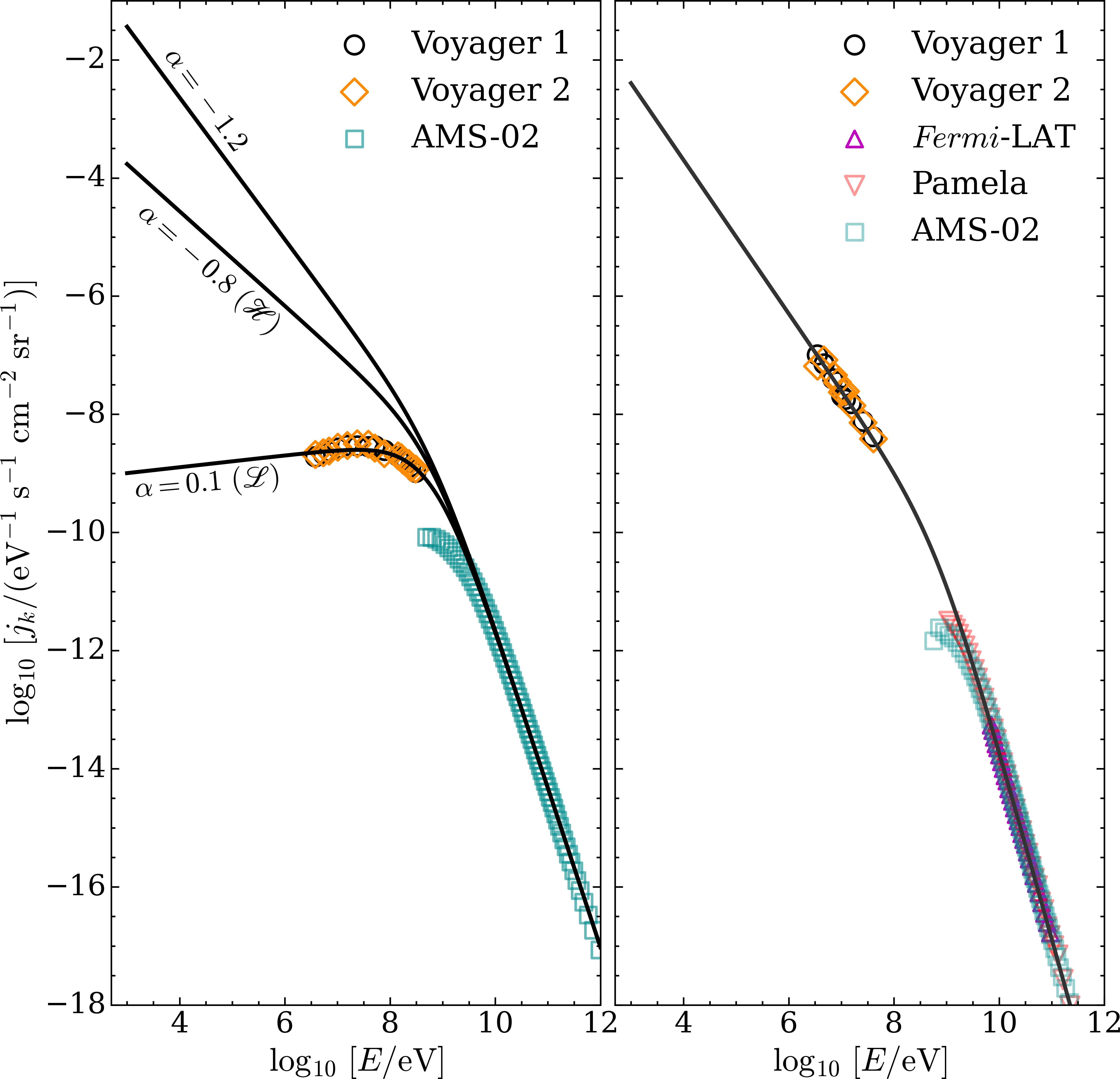
Figure 3: Left panel: CR proton spectrum as a function of the energy for three low-energy spectral slope: $\alpha=0.1$ (labelled as model $\mathscr{L}$), $\alpha=-0.8$ (labelled as model $\mathscr{H}$), and $\alpha=-1.2$. Right panel: CR electron spectrum as a function of the energy. Data: Voyager 1 (black circles, Cummings et al., 2016); Voyager 2 (orange diamonds, Stone et al., 2019); Fermi-LAT (magenta up-pointing triangles, Ackermann et al., 2010); Pamela (pink down-pointing triangles, Adriani et al., 2011); AMS-02 (cyan squares, Aguilar et al., 2014, 2015).

Table 2: Parameters of the interstellar CR electron and proton spectra, Eq. (2), where $E$ is in MeV and $C$ is in units of eV^-1 s^-1 cm^-2 sr^-1.

Species $k$	$C$	$E_{0}\leavevmode\nobreak\ [{\rm MeV}]$	$\alpha$	$\beta-\alpha$
$e$	$2.1\times 10^{18}$	710	$-1.3$	3.2
$p$ (model $\mathscr{L}$)	$2.4\times 10^{15}$	650	0.1	2.7
$p$ (model $\mathscr{H}$)	$2.4\times 10^{15}$	650	$-0.8$	2.7

In this work we are interested in H₂ column densities typical of molecular cloud cores ($N_{\rm H_{2}}\lesssim 10^{23}$ cm^-2), so we first need to determine how the spectrum of interstellar CRs is attenuated as it propagates within a molecular cloud. In this column density regime, it holds the so-called continuous slowing down approximation, according to which a CR propagates along a magnetic field line and, each time it collides with an H₂ molecule, loses a negligible amount of energy compared to its initial energy. Thus, we assume a free-streaming regime of propagation of CRs (Padovani et al., 2009), neglecting their possible resonance scattering off small-scale turbulent fluctuations, which then may lead to diffusive propagation. Therefore, the spectrum of CR particles of species $k$ propagated at a column density $N_{\rm H_{2}}$, $j_{k}(E,N_{\rm H_{2}})$, can be expressed as a function of the interstellar CR spectrum at the nominal column density $N_{\rm H_{2}}=0$, $j_{k}(E_{0},0)$, as

$$j_{k}(E,N_{\rm H_{2}})=j_{k}(E_{0},0)\frac{L_{k}(E_{0})}{L_{k}(E)}\,,$$ (3)

where $E$ is the energy of a CR particle with initial energy $E_{0}$ after passing through a column density $N_{\rm H_{2}}$ given by

$$N_{\rm H_{2}}=-\int_{E_{0}}^{E}\frac{{\rm d}E}{L_{k}(E)}\,.$$ (4)

The most updated energy loss function for protons colliding with H₂ is presented in Padovani et al. (2018b).

The lower left panel of Fig. 4 shows the spectra of CR protons for both models $\mathscr{L}$ and $\mathscr{H}$ at four different column densities (from $10^{20}$ to $10^{23}$ cm^-2). The lower right panel shows the corresponding spectra of secondary electrons computed following the procedure described in Ivlev et al. (2021). We also plot the spectra of CR primary electrons since their contribution to the CR ionisation rate is non-negligible when considering proton spectra with $\alpha\gtrsim-0.4$. For example, for model $\mathscr{L}$, at $N_{\rm H_{2}}=10^{20}$ cm^-2 and $10^{21}$ cm^-2, the contribution of CR primary electrons to the CR ionisation rate is a factor of 6 and 2 larger, respectively, than that of CR protons. At $10^{22}$ cm^-2 electron and proton ionisation rates are comparable, while at larger column densities, protons dominate (see also the lower panel of Fig. 5).

Additionally, we use the model of Ivlev et al. (2021) to compute the secondary electron spectrum from primary CR electrons. As for the latter, we find their contribution to ionisation to be non-negligible for $\alpha\gtrsim-0.4$ (see Sect. 3). As shown in the lower right panel inset of Fig. 4, the spectrum of secondary electrons produced by primary CR electrons is higher by a factor of $\simeq 10$, 3.4, and 1.6 (at H₂ column densities of $10^{20}$, $10^{21}$, and $10^{22}$ cm^-2, respectively) than that of the secondaries produced by protons for model $\mathscr{L}$.

In contrast to the findings of Cravens & Dalgarno (1978), according to which the spectrum of secondaries has an average energy of about 30 eV, the theory developed by Ivlev et al. (2021) predicts that the spectrum of secondaries is distributed over a wide range of energies (see Appendix B for more detailed discussion).

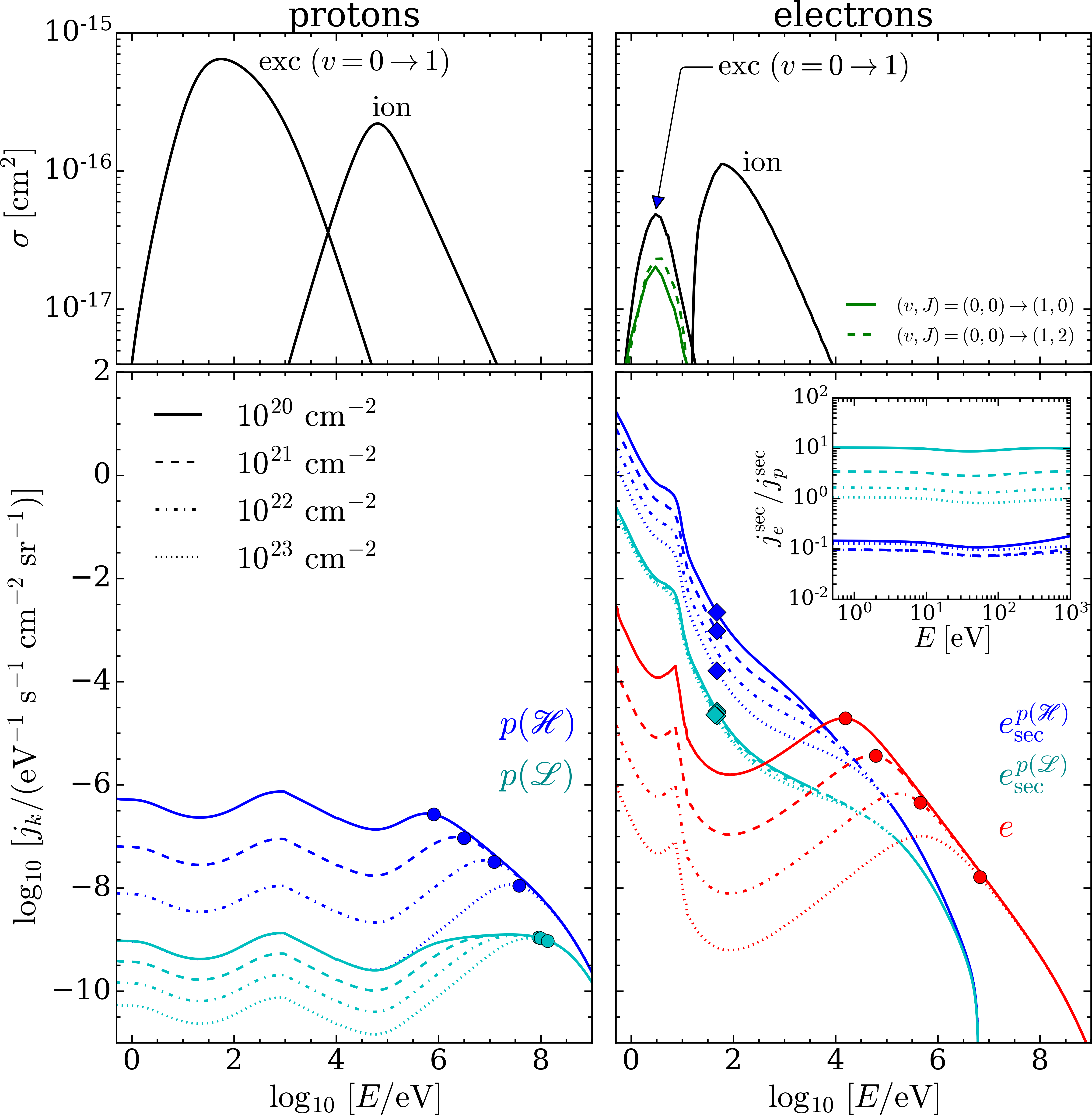
Figure 4: Upper panels: vibrational excitation, $v=0\rightarrow 1$, and ionisation (“ion”) cross sections for protons (left plot; Tabata & Shirai 2000 and Rudd et al. 1992, respectively) and for electrons (right plot; Yoon et al. 2008 and Kim et al. 2000, respectively) colliding with H₂. Solid and dashed green lines show the rovibrational cross sections $(v,J)=(0,0)\rightarrow(1,0)$ and $(v,J)=(0,0)\rightarrow(1,2)$, respectively, from the MCCC calculations. Lower panels: CR spectra at the column densities $N_{\rm H_{2}}=10^{20}$, $10^{21}$, $10^{22}$, and $10^{23}$ cm^-2 as a function of the energy; left plot: CR protons (model $\mathscr{L}$ and $\mathscr{H}$; cyan and blue lines, respectively); right plot: CR primary electrons ($e$; red lines) and secondary electrons from CR protons (model $\mathscr{L}$ and $\mathscr{H}$, labelled as $e_{\rm sec}^{p(\mathscr{L})}$ and $e_{\rm sec}^{p(\mathscr{H})}$, respectively; cyan and blue lines). The inset shows the ratio between the secondary electron spectra generated by primary CR electrons, $j_{e}^{\rm sec}$, and by CR protons, $j_{p}^{\rm sec}$ (same colour- and line-coding of the main plot). Solid circles (diamonds) in lower panels denote the energies of primary CRs (secondary electrons) that contribute most to the CR ionisation rate (see also Appendix B).

3 Cosmic-ray excitation and ionisation rates

The upper panels of Fig. 4 show the excitation and ionisation cross sections that we adopt to calculate the corresponding rates,

$$\zeta_{k}(N_{\rm H_{2}})=2\pi\ell\int j_{k}(E,N_{\rm H_{2}})\sigma_{k}(E){\rm d}E\,.$$ (5)

Here, $\sigma_{k}$ is the excitation or ionisation cross section, and $k$ is the species considered (CR protons, primary CR electrons, and secondary electrons) colliding with H₂. Assuming a semi-infinite slab geometry, $\ell=1$ for primary CRs and $\ell=2$ for secondary electrons, since the latter are produced locally and propagate almost isotropically (see Padovani et al., 2018a). Then, the total ionisation and excitation rates per H₂ molecule are the sum of the individual contributions given by Eq. (5).

As mentioned at the beginning of Sect. 2, we calculate the electron excitation rates, $\zeta_{{\rm exc},u}$, where $u$ refers to the upper $J$ level, of the rovibrational transitions $(v,J)=(0,0)\rightarrow(1,0)$ and $(0,0)\rightarrow(1,2)$. Bialy (2020) estimated the ratio between excitation and ionisation rates from the excitation probabilities calculated by Gredel & Dalgarno (1995) for 30 eV monoenergetic electrons. Here, we use the H₂ excitation cross sections calculated with the MCCC method (see the solid and dashed green curves in the upper right plot of Fig. 4), and the spectra of primary and secondary electrons computed in the previous section. The excitation rates for these two transitions are shown in the upper panel of Fig. 5. In particular, we show the excitation rates as a function of the H₂ column density for different low-energy spectral slope, $\alpha$, of the CR proton spectrum. We consider not only the models $\mathscr{L}$ and $\mathscr{H}$ described before, with $\alpha=0.1$ and $\alpha=-0.8$, respectively, but allow $\alpha$ to vary from $-1.2$ to $0.1$. As shown by Fig. 11, $\alpha=-1.2$ gives a CR ionisation rate that represents the upper envelope of the values estimated from observations of diffuse clouds, while $\alpha=-0.8$ results in a rate in agreement to average value of the sample. Values of $\alpha\gtrsim-0.4$ give a rate below the lower envelope of observational estimates of $\zeta_{\rm ion}$ in diffuse clouds.

We also verify that the excitation rate due to CR protons is negligible. Since rotationally-resolved proton-impact cross sections are not available, we use the vibrational transition $(v,v^{\prime})=(0,1)$ cross section summed over all rotational levels recommended by Tabata & Shirai (2000) to obtain an upper limit to the H₂ excitation rate by CR protons. Their contribution turns out to be more than three orders of magnitude smaller than that of secondary electrons, therefore it can be safely neglected. This is because already at column densities of the order of $10^{20}$ cm^-2, protons with energies below about 1 MeV are stopped (see Fig. 2 in Padovani et al., 2018b). This implies that the CR proton spectrum is very small at the energies where the excitation cross section has its maximum ($\sim 100$ eV; see upper left panel of Fig. 4).

Excitation by primary CR electrons can also be neglected, since excitation cross sections peak at $\sim 3$–4 eV, and at these energies the spectra of secondary electrons generated by protons are up to $\sim 3$ orders of magnitude higher than the primary CR electron spectrum (see the middle right panel of Fig. 4). However, while primary CR electrons can be neglected, secondary electrons produced by primary CR electrons make a non-negligible contribution to the total excitation rate if $\alpha\gtrsim-0.4$ (see the red lines in the upper panel of Fig. 5).

The lower panel of Fig. 5 shows the ionisation rate due to CR protons and primary CR electrons as a function of column density $N_{\rm H_{2}}$, including the contribution of the corresponding secondary electrons, labelled as $p+e_{\rm sec}^{p}$ and $e+e_{\rm sec}^{e}$, respectively. Here, the contribution of $e+e_{\rm sec}^{e}$ is not negligible for $\alpha\gtrsim-0.4$. In particular, the contribution to ionisation of $e_{\rm sec}^{e}$ is larger than that of primary CR electrons and increases with H₂ column density. Specifically, the ratio of $\zeta_{\rm ion}$ due to $e_{\rm sec}^{e}$ and to $e$ is equal to about 1.3, 1.5, 1.7, and 1.9 at $N_{\rm H_{2}}=10^{20}$, $10^{21}$, $10^{22}$, and $10^{23}$ cm^-2, respectively. Similarly to the excitation rate, primary CR electrons, together with their secondaries, determine a lower limit for $\zeta_{\rm ion}$ expected from the observations, independently on the assumed value of $\alpha$. We note, however, that in Fig. 11 there are ionisation rate data below those expected from this limit. This can likely be explained by invoking the presence of highly twisted magnetic field lines, so that the effective column density passed through by CRs may be much higher than that along the line of sight (Padovani et al., 2013). Thus the CR spectrum could be strongly attenuated and the corresponding $\zeta_{\rm ion}$ may be smaller than predicted.

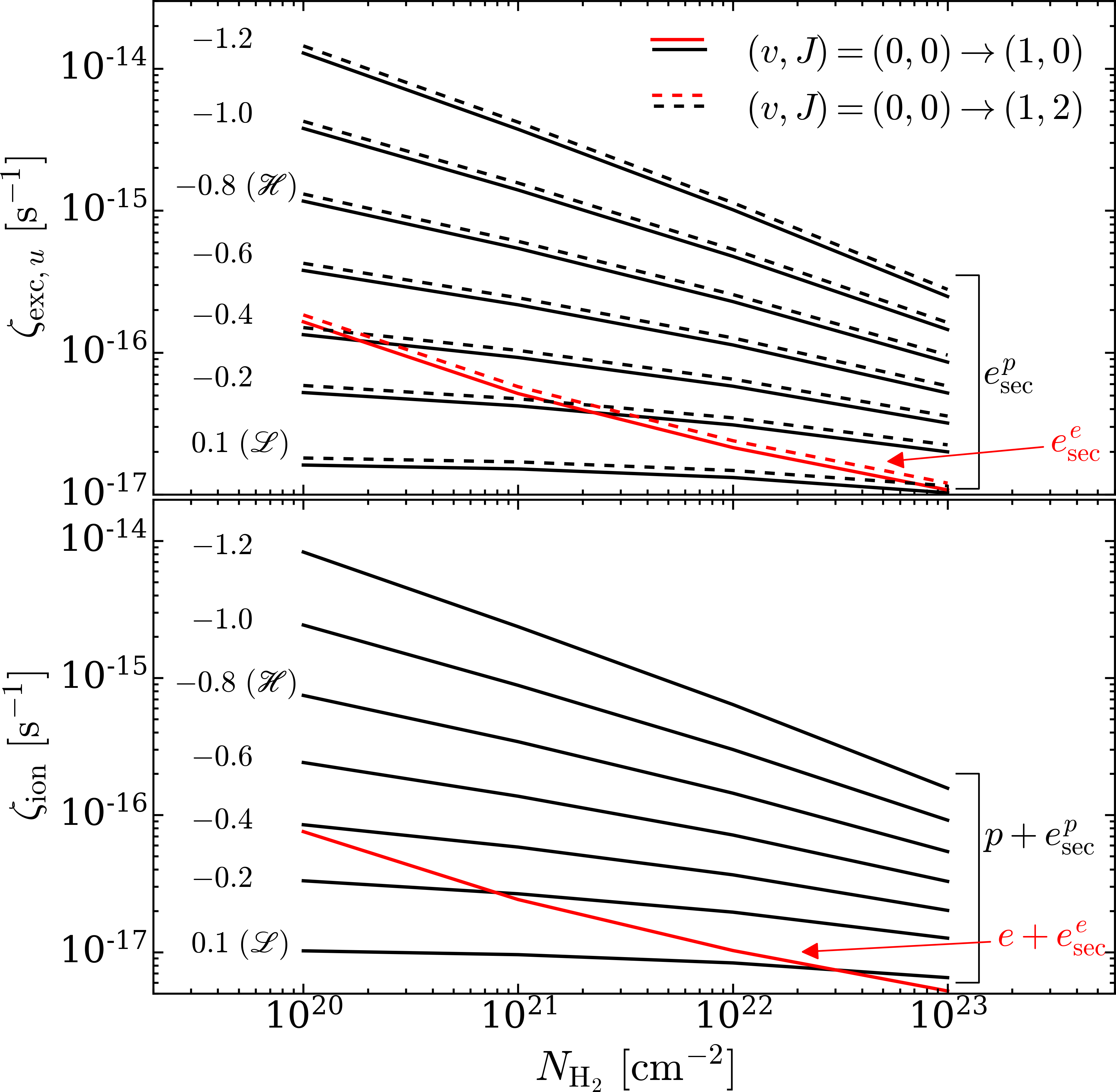
Figure 5: Upper panel: CR excitation rate due to secondary electrons as a function of H₂ column density for the H₂ rovibrational transitions $(v,J)=(0,0)\rightarrow(1,0)$ and $(v,J)=(0,0)\rightarrow(1,2)$ (solid and dashed lines, respectively). Black (red) lines show the rates due to secondaries produced by CR protons, $e_{\rm sec}^{p}$ (primary CR electrons, $e_{\rm sec}^{e}$). Lower panel: CR ionisation rate due to CR protons (solid black lines) and CR electrons (solid red line). All the curves include the contribution to ionisation due to the corresponding generation of secondary electrons. Labels on the left in both panels denote the low-energy spectral slope (parameter $\alpha$ in Eq. (2)). The cases $\alpha=0.1$ and $\alpha=-0.8$ correspond to model $\mathscr{L}$ and $\mathscr{H}$, respectively.

Finally, Fig. 6 shows the ratio between the excitation and ionisation rates for the rovibrational transitions under consideration. We note that, while in Fig. 5 the contributions of the various species to excitation and ionisation are shown separately, here we show the ratio of the total rates. We find that for increasing H₂ column densities and increasingly negative low-energy spectral slopes $\alpha$, $\zeta_{{\rm exc},u}/\zeta_{\rm ion}$ tends to an almost constant value of $\simeq 1.6$ and 1.8, for the $(v,J)=(0,0)\rightarrow(1,0)$ and $(v,J)=(0,0)\rightarrow(1,2)$ transitions, respectively. For $\alpha\gtrsim-0.4$, $\zeta_{{\rm exc},u}/\zeta_{\rm ion}$ reaches larger values because of the significant contribution of secondary electrons from primary CR electrons to the excitation rate (see Fig. 5). Bialy (2020) assumed the ratio between the total excitation rate (summed over the upper levels) and the ionisation rate to be equal to 5.8. Looking at Fig. 6, we see that the $\alpha$- and $N_{\rm H_{2}}$-dependent value, adding up the excitation rates of the two upper levels considered, ranges from 3.3 to 4.4. However, results are not directly comparable as in the present work we also consider the excitation due to secondary electrons from primary CR electrons and the contribution to ionisation due to both primary CR electrons and their secondaries.

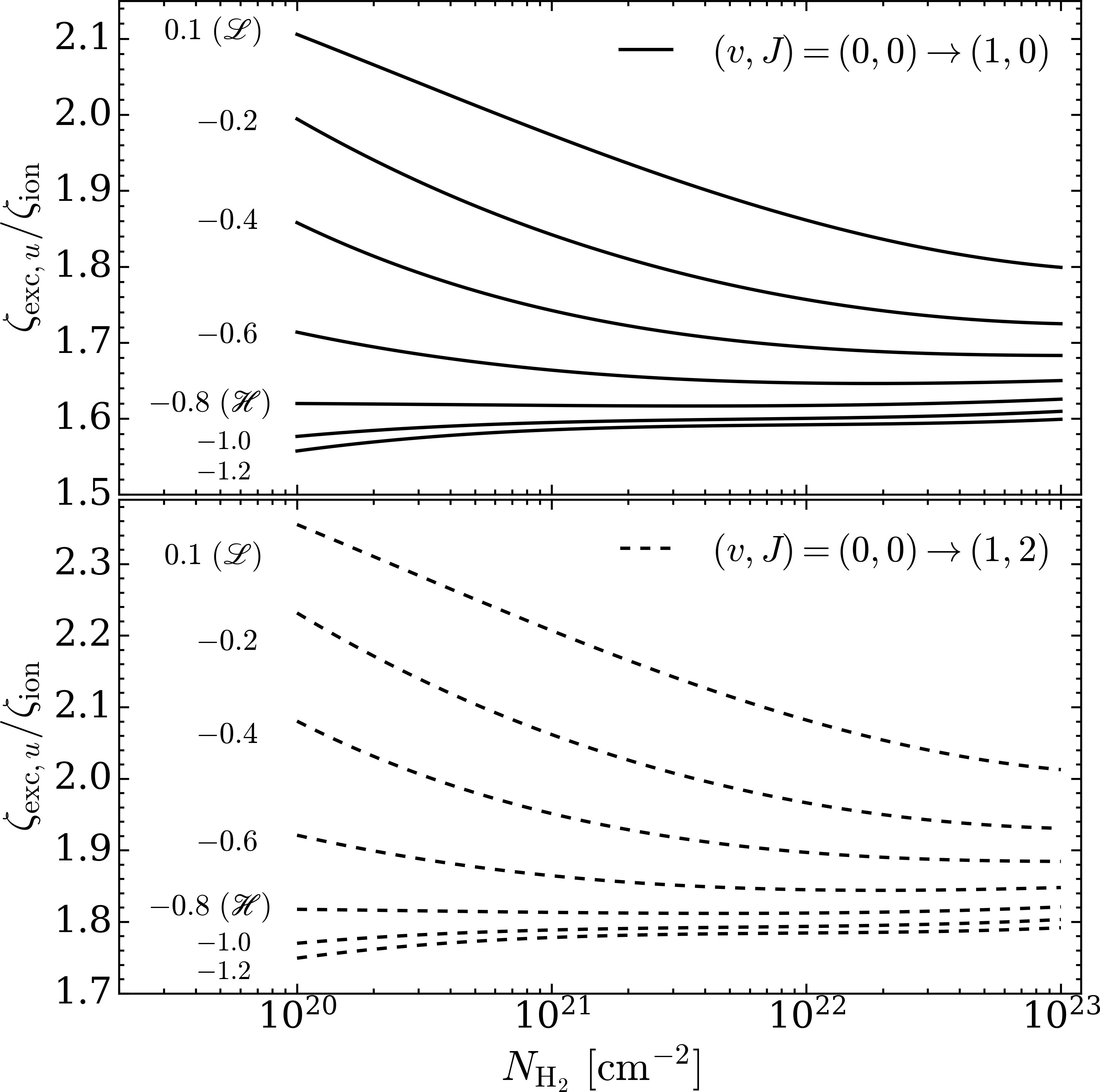
Figure 6: Ratio between the total CR excitation and ionisation rates as a function of H₂ column density for the H₂ rovibrational transitions $(v,J)=(0,0)\rightarrow(1,0)$ and $(v,J)=(0,0)\rightarrow(1,2)$ (upper and lower panel, respectively). Labels on the left denote the spectral energy slope at low energy (parameter $\alpha$ in Eq. (2)). The cases $\alpha=0.1$ and $\alpha=-0.8$ correspond to model $\mathscr{L}$ and $\mathscr{H}$, respectively.

4 Line excitation

As shown in Fig. 7, several mechanisms contribute to the population of the $(v,J)=(1,0)$ and $(1,2)$ rovibrational levels. These levels are populated directly by CRs (blue arrows), more precisely by secondary electrons (see also Sect. 3). Population also occurs through indirect processes (black arrows). Singlet $B\,^{1}\Sigma_{u}^{+}$ and $C\,^{1}\Pi_{u}$ electronic states can be excited both radiatively by interstellar UV photons and collisionally by CRs (magenta arrow). The excited electronic states rapidly decay into bound rovibrational levels of the electronic ground state, emitting in the Lyman-Werner bands (Sternberg, 1988). A further indirect population process occurs as a side-product of H₂ formation on grains (orange arrow). Part of the binding energy is redistributed to the internal excitation of the newly formed H₂, mainly in the vibrational levels $2\leq v\leq 5$ (Islam et al., 2010). Other fractions of the binding energy are converted into dust grain heating and into kinetic energy of H₂. Subsequent decay populates the lower $v=1$ level (Black & van Dishoeck, 1987).

We summarise below the equations to compute the expected energy surface brightness (hereafter “brightness”) induced by CRs, UV photons, and the H₂ formation process, referring to Bialy (2020) for further details. The derivation of the contributions to line intensities by CRs are similar to those presented in Bialy (2020). However, we consider the more general case where $\zeta_{\rm ion}$ is not constant and thus appears in the integrals. For more details and limiting cases, see Appendix B in Bialy et al. (2021). Equations are given for a generic mixture of hydrogen in atomic and molecular form, thus the brightness is a function of the total column density of hydrogen in all its forms, $N=N_{\rm H}+2N_{\rm H_{2}}$, where $N_{\rm H}$ and $N_{\rm H_{2}}$ are the atomic and molecular H₂ column densities, respectively. Since we are mainly interested in molecular cloud cores, in the following we assume $N\approx 2N_{\rm H_{2}}$. Consequently, the fraction of molecular hydrogen with respect to the total, $x_{\rm H_{2}}=n_{\rm H_{2}}/(n_{\rm H}+2n_{\rm H_{2}})$, where $n_{\rm H}$ and $n_{\rm H_{2}}$ are the volume densities of H and H₂, respectively, is set to 1/2.

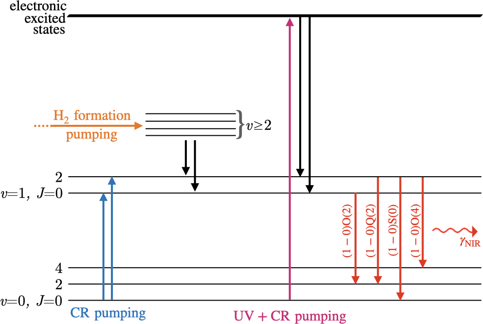
Figure 7: Sketch of the excitation mechanisms contributing to the population of the $(v,J)=(1,0)$ and $(1,2)$ levels. Direct population is due to CRs (blue arrows) and indirect population (black arrows) occur from the decay of electronic excited states previously populated by radiative excitation of interstellar UV photons and by collisional excitation by CRs (magenta arrow) and from the decay of higher vibrational levels ($v\geq 2$) formerly populated as a by-product of the H₂ formation process (orange arrow). The four red arrows show the near-infrared (NIR) transitions listed in Table 1. We magnify the region of $v=0,1$ levels for clarity.

4.1 Direct excitation by secondary CR electrons

The expected brightness of the individual line with upper and lower levels $u$ and $l$ due to CR excitation is

$$I_{ul}^{\rm dir}(N)=\alpha_{ul}\frac{E_{ul}}{4\pi}\int_{0}^{N}\zeta_{{\rm exc},u}(N^{\prime})e^{-\tau_{d}(N^{\prime})}x_{\rm H_{2}}(N^{\prime}){\rm d}N^{\prime}\,,$$ (6)

where $\tau_{d}=\sigma_{d}N$ is the optical depth for dust extinction and $\sigma_{d}\approx 4.5\times 10^{-23}$ cm² is the cross section per hydrogen nucleus averaged over $2-3\leavevmode\nobreak\ \mu$m (Draine, 2011; Bialy, 2020). Here, $\alpha_{ul}$ is the probability to decay to state $l$ given state $u$ is excited and $E_{ul}$ is the transition energy (see Table 1 in Bialy 2020). We note that H₂ self-absorption is negligible with respect to the absorption by dust at these wavelengths.

4.2 Indirect excitation by interstellar and CR-induced UV photons

The expected brightness due to interstellar UV photons and CR-excited Lyman-Werner (LW) transitions is

$$I_{ul}^{\rm LW}(N)=f_{ul}^{\rm LW}\frac{\bar{E}_{\rm UV}}{4\pi}[\mathcal{E}^{\rm LW}_{\rm ISRF}(N)+\mathcal{E}^{\rm LW}_{\rm CR}(N)]$$ (7)

where

$$\mathcal{E}^{\rm LW}_{\rm ISRF}(N)=\int_{0}^{N}P_{0}\chi_{a}(N^{\prime})x_{\rm H_{2}}(N^{\prime}){\rm d}N^{\prime}$$ (8)

and

$$\mathcal{E}^{\rm LW}_{\rm CR}(N)=\mathcal{E}^{\rm LW}_{\rm CR,0}(\omega,R_{\rm V})\left[\frac{\zeta_{\rm ion}(N)}{10^{-17}\leavevmode\nobreak\ {\rm s}^{-1}}\right]$$ (9)

are the total UV emission rates per unit area resulting from the decay of the $B\,^{1}\Sigma_{u}^{+}$ and $C\,^{1}\Pi_{u}$ states excited by the UV interstellar radiation field (ISRF) and CRs, respectively. Here, $P_{0}\simeq 9D_{0}$ is the unattenuated UV pumping rate (Bialy, 2020), $D_{0}=2\times 10^{-11}G_{0}$ s^-1 is the unattenuated photodissociation rate (Draine & Bertoldi, 1996, assuming a semi-infinite slab geometry), $G_{0}$ is the far-UV radiation field in Habing units (Habing, 1968), and $\chi_{a}(N)=f_{\rm sh}\exp[-\tau_{g}(N)]$ accounts for the self-shielding effect of H₂ and dust extinction. The H₂ self-shielding function is given by Draine & Bertoldi (1996)

$$f_{\rm sh}=\frac{a_{1}}{(1+x/b_{5})^{2}}+\frac{a_{2}}{\sqrt{1+x}}\exp\left(-a_{3}\sqrt{1+x}\leavevmode\nobreak\ \right)\,,$$ (10)

where $a_{1}=0.965$, $a_{2}=0.035$, $a_{3}=8.5\times 10^{-4}$, $x=N_{\rm H_{2}}/(5\times 10^{14}\leavevmode\nobreak\ {\rm cm^{-2}}$), and $b_{5}$ is the absorption-line Doppler parameter normalised to $10^{5}\leavevmode\nobreak\ {\rm cm\leavevmode\nobreak\ s^{-1}}$. We set $b_{5}=2$ as in Bialy & Sternberg (2016). Finally, $\tau_{g}=\sigma_{g}N$, where $\sigma_{g}=1.9\times 10^{-21}$ cm² is the average value of the far-UV dust grain absorption cross section for solar metallicity (Draine, 2011). We recall that we assume $N=2N_{\rm H_{2}}.$ The total CR-induced UV emission rate per unit area, $\mathcal{E}^{\rm LW}_{\rm CR}$, is given by Cecchi-Pestellini & Aiello (1992) (see also Ivlev et al., 2015), where

$$\mathcal{E}^{\rm LW}_{\rm CR,0}(\omega,R_{\rm V})\simeq\frac{960}{1-\omega}\left(\frac{R_{\rm V}}{3.2}\right)^{1.5}\leavevmode\nobreak\ {\rm cm^{-2}\leavevmode\nobreak\ s^{-1}}\,.$$ (11)

Here, $\omega$ is the dust albedo at UV wavelengths and $R_{\rm V}$ is a measure of the extinction at visible wavelengths (Draine, 2011). Finally, $\bar{E}_{\rm UV}\simeq 1.82$ eV is the effective transition energy and $f_{ul}^{\rm LW}$ is the relative emission of the transition from level $u$ to level $l$ (see Sternberg 1988 and Table 1 in Bialy 2020). We find that $\mathcal{E}^{\rm LW}_{\rm CR}\ll\mathcal{E}^{\rm LW}_{\rm ISRF}$ at any column density, thus we can safely neglect the contribution of the term in Eq. (9) to $I_{ul}^{\rm LW}$ (Eq. (7)).

4.3 Indirect excitation from H₂ formation

The expected brightness due to H₂ formation pumping is

$$I_{ul}^{\rm f}(N)=f_{ul}^{\rm f}\frac{\bar{E}_{\rm f}}{4\pi}[\mathcal{E}^{\rm f}_{\rm ISRF}(N)+\mathcal{E}^{\rm f}_{\rm CR}(N)]\,,$$ (12)

where the two terms on the right-hand side represent the total emission rates per unit area due to the destruction of H₂ by interstellar UV photons and by CRs, respectively. They are given by

$$\mathcal{E}^{\rm f}_{\rm ISRF}(N)=\int_{0}^{N}D_{0}\chi_{a}(N^{\prime})x_{\rm H_{2}}(N^{\prime}){\rm d}N^{\prime}$$ (13)

and

$$\mathcal{E}^{\rm f}_{\rm CR}(N)=\int_{0}^{N}(y+\Phi_{\rm diss})\zeta_{\rm ion}(N)e^{-\tau_{d}(N)}x_{\rm H_{2}}(N){\rm d}N\,.$$ (14)

Here, $\bar{E}_{\rm f}\simeq 1.3$ eV corresponds to the excitation of the $v=4$ level (Islam et al., 2010), the relative emission of the transition from level $u$ to level $l$, $f_{ul}^{\rm f}$, is determined by the formation excitation pattern (see Black & van Dishoeck 1987 and Table 1 in Bialy 2020), $y\simeq 2$ accounts for additional removal of H₂ by H${}_{2}^{+}$ in predominantly molecular gas (Bialy & Sternberg, 2015), and $\Phi_{\rm diss}\simeq 0.7$ accounts for the fact that H₂ can also be destroyed through dissociation in addition to ionisation (Padovani et al., 2018a).

5 A look-up plot for $\zeta_{\rm ion}$ and $\alpha$

Figure 8 shows the expected brightness for direct excitation by secondary electrons and indirect excitation by UV photons, for the four rovibrational transitions listed in Table 1. The contribution of H₂ formation pumping is not shown because it is smaller by a factor 20 to 200 than that of direct CR excitation (depending on the transition considered), so it can be safely neglected. A similar conclusion was obtained by Bialy (2020), see their Fig. 1. For a UV field equal to the mean interstellar field ($G_{0}=1.7$), CRs dominate the excitation if the observed brightness is larger than about $10^{-8}$ erg cm^-2 s^-1 sr^-1, for column densities higher than about a few times $10^{21}$ cm^-2, depending on the transition.

Figure 8 provides a look-up plot for a direct estimate of $\zeta_{\rm ion}$, overcoming the uncertainties of other observational methods (see Sect. 1). We also note that the simultaneous observation of several transitions provides more stringent constraints on $\zeta_{\rm ion}$. With this diagram, it is also possible to determine the slope of the CR proton spectrum at low energies and to compare it to measurements by the Voyager spacecrafts ($\alpha=0.1$). We remind the reader that, using our model for CR propagation and generation of secondary electrons, we relate the CR ionisation rate in the cloud to the unattenuated CR proton spectrum impinging upon the cloud, which is characterised by a low-energy spectral slope $\alpha$ (see Sect. 2.3). In order to facilitate the usage of Fig. 8, we have developed a publicly available web-based application that allows a more accurate value of the ionisation rate and of the low-energy spectral slope to be obtained, given the line brightness and the corresponding column density.

The expected brightness in Fig. 8 applies to typical interstellar UV fields ($G_{0}=1.7$) and to the average interstellar CR spectrum based on measurements in the solar neighbourhood. However, different regions of dense gas are likely to be dominated by local conditions, such as perturbations in the magnetic field structure or shocks. This could cause variations in the shape of the CR spectrum. For example, in the vicinity of protostars, the UV field can be much more intense ($G_{0}\gg 1$), especially close to shocks (e.g. Hollenbach & McKee, 1989; Karska et al., 2018). However, in the same shocks, e.g. along a protostellar jet or on the surface of a protostar, it is also possible to locally accelerate CRs (Padovani et al., 2015, 2016; Gaches & Offner, 2018; Padovani et al., 2021b), and therefore even more intense H₂ lines should be observed. Consequently, this technique could also be used to further confirm the enhanced ionisation triggered by local CRs expected in star-forming regions.

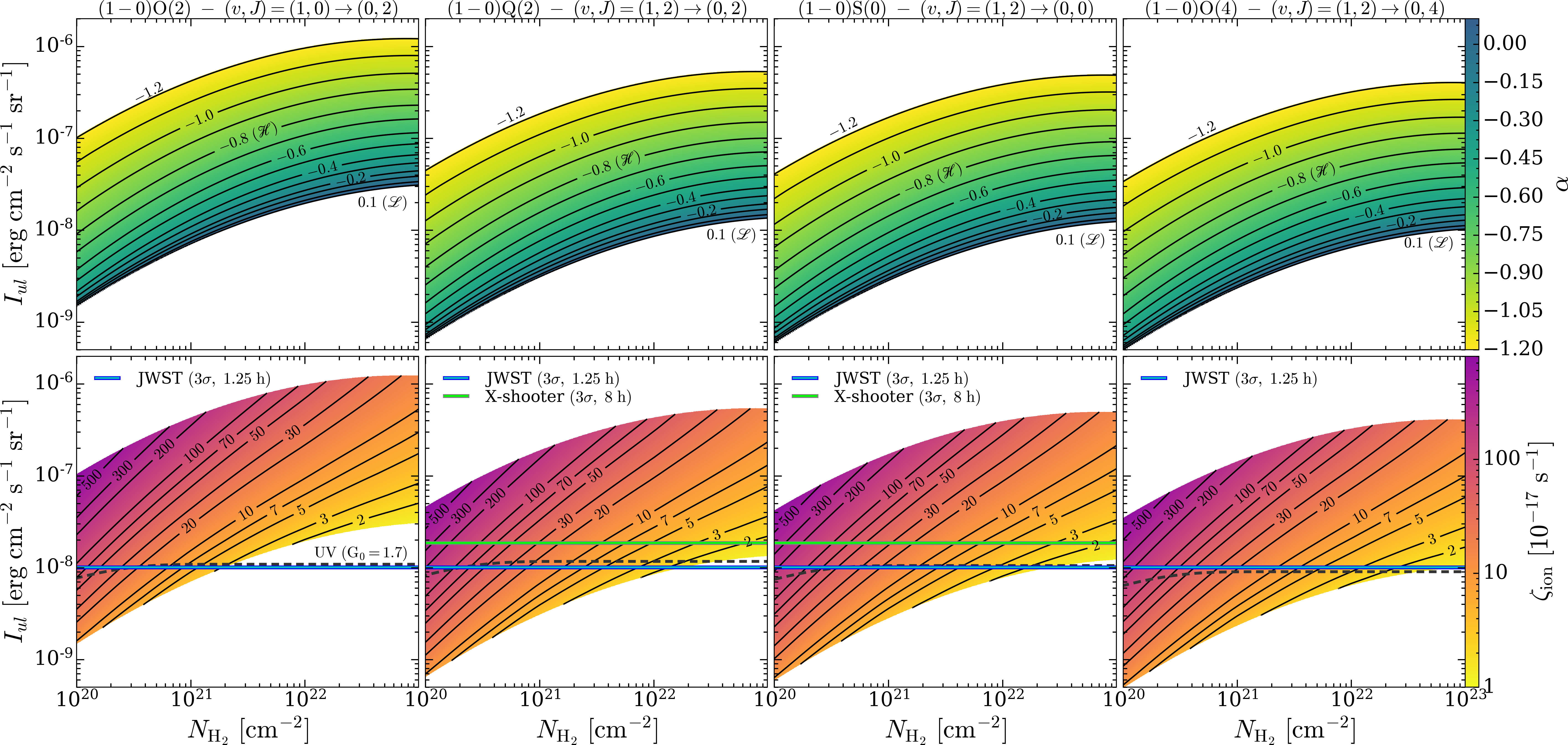
Figure 8: Maps of the the low-energy spectral slope ($\alpha$, upper row) and of the CR ionisation rate ($\zeta_{\rm ion}$, lower row) as a function of the energy surface brightness expected by direct CR excitation for the four H₂ rovibrational transition listed in Table 1 and of the H₂ column density. We note that we assume $N=2N_{\rm H_{2}}$. The dashed black lines show the expected brightness due to indirect excitation by interstellar UV photons for a far-UV radiation field with $G_{0}=1.7$ (Draine, 2011). Solid black lines show the iso-contours of $\alpha$ (upper panels) and $\zeta_{\rm ion}$ in units of $10^{-17}$ s^-1 (lower panels). Solid blue horizontal lines show the JWST sensitivity for a signal-to-noise ratio of 3 over 1.25 h of integration, adding up the signal over 50 shutters. Solid green horizontal lines show the X-Shooter sensitivity for a signal-to-noise ratio of 3 over 8 h of integration, adding up the signal over the whole slit.

Bialy (2020) showed that X-shooter can be used to observe the $(1-0){\rm Q}(2)$ and $(1-0){\rm S}(0)$ lines of H₂. One of the limitations of X-shooter is the small size of the slits ($11^{\prime\prime}\times 0.4^{\prime\prime}$), which allow only a small portion of a starless core to be observed, whose typical size is of the order of 0.1 pc. Unfortunately, the brightest H₂ rovibrational line, $(1-0){\rm O}(2)$, cannot be observed from the ground due to atmospheric absorption, while the $(1-0){\rm O}(4)$ transition falls outside the range of frequencies observable by X-shooter. Bialy et al. (2021) recently employed this new method for the determination of $\zeta_{\rm ion}$ using MMIRS mounted on MMT, obtaining for five dense molecular clouds upper limits on the $(1-0){\rm S}(0)$ transition and the CR ionisation rate (of the order of $10^{-16}$ s^-1, see also Appendix C). These observations successfully confirmed the validity of this method, setting the ground for future observations with JWST.

The NIRSpec instrument mounted on JWST turns out to be the crucial facility for observing these H₂ infrared lines. Indeed, in addition to making it possible to observe all four H₂ transitions in Table 1, NIRSpec used in multi-object spectroscopy mode provides slits with an angular extent of $3.4^{\prime}$ and a width of $0.27^{\prime\prime}$. Adding up the signal over 50 shutters, the $3\sigma$ threshold is achieved in only 1.25 h of observation (see Bialy et al., 2021, for more details). Given the high spatial resolution, this also means that for a starless core such as Barnard 68, at a distance of 125 pc (de Geus et al., 1989), it is possible to obtain about 10 independent estimates of the brightness, and hence of $\zeta_{\rm ion}$, across the core.

Therefore, in principle it will be possible to obtain for the first time the spatially-resolved distribution of the CR ionisation rate in a starless core and not a single estimate of $\zeta_{\rm ion}$ as obtained through the methods described in Sect. 1. An important consequence is the possibility of testing the presence of a gradient of $\zeta_{\rm ion}$, predicted by models of attenuation of the interstellar CR spectrum as CRs propagate through a molecular cloud (Padovani et al., 2009; Padovani & Galli, 2011; Padovani et al., 2013, 2018b; Silsbee et al., 2018; Silsbee & Ivlev, 2019), or whether $\zeta_{\rm ion}$ is nearly spatially uniform, in case CRs are accelerated inside a cloud by magnetic reconnection events (Gaches et al., 2021).

Lower panels of Fig. 8 also show the $3\sigma$ limit for 8 h of integration with X-shooter and 1.25 h of integration with JWST.

6 Conclusions

In this paper we presented a detailed numerical method to test and extend the analytic model by Bialy (2020). Our modelling allows a robust estimate of the CR ionisation rate, $\zeta_{\rm ion}$, and of the low-energy spectral slope of the CR proton spectrum, $\alpha$, in dense molecular clouds from the observation of photons emitted at near-infrared wavelengths by the decay of rovibrational levels of molecular hydrogen. This technique allows to quantify $\zeta_{\rm ion}$ independently on any chemical network.

In a molecular cloud, when sufficiently far away from UV sources such as a protostar, the excitation of the $(v,J)=(1,0)$ and $(1,2)$ levels of H₂ is dominated by secondary CR electrons. It is traditionally assumed that the spectrum of secondary CR electrons has an average energy of about 30 eV (Cravens & Dalgarno, 1978). However, the spectrum of secondary electrons produced during the propagation of primary CRs (both protons and electrons) can be computed accurately at the energies of interest (Ivlev et al., 2021). In addition, rigorous theoretical calculations of electron-impact excitation cross sections of rovibrational levels of H₂ are now available (Scarlett et al., 2021a).

Finally, following Bialy (2020), we computed the expected brightness for the H₂ transitions listed in Table 1. We then presented a look-up plot, accompanied by an interactive on-line tool, that allows to obtain a straightforward estimate of $\zeta_{\rm ion}$ and $\alpha$, given the brightness of an H₂ transition and the corresponding column density. The feasibility of this type of observation was recently verified by Bialy et al. (2021) using the spectrograph MMIRS mounted on the MMT, obtaining upper limits for $\zeta_{\rm ion}$ in five dense molecular clouds. However, it will be the new generation instrument JWST that will allow the application of this technique with a great improvement in terms of sensitivity and spatial resolution, leading in principle to an actual line detection. In fact, while today the current methods provide a single CR ionisation rate estimate per observed source, JWST will allow to derive the CR ionisation rate profile through a starless core with a single pointing. For example, with 1.25 h of observation with JWST, up to about 10 independent $\zeta_{\rm ion}$ estimates can be derived with a $3\sigma$ sensitivity. In addition to having major implications on the interpretation of the chemical composition of a molecular cloud and its dynamical evolution, the determination of $\alpha$ and of the profile of $\zeta_{\rm ion}$ will also make it possible to test the predictions of models of CR propagation in molecular clouds (e.g. Everett & Zweibel, 2011; Morlino & Gabici, 2015; Silsbee & Ivlev, 2019; Padovani et al., 2020; Gaches et al., 2021).

Appendix A Energy loss function for electrons in helium

The upper panel of Fig. 9 summarises the excitation and ionisation cross sections that we use to derive the energy loss function for electrons colliding with He atoms. The equation for calculating the loss function is identical to Eq. (2.2), except for the pre-factor of the momentum transfer term, where $m_{\rm H_{2}}$ is replaced by $m_{\rm He}$. In the lower panel of the same figure we compare the H₂ and He energy loss functions. We note that, by considering a medium with $\sim 20\%$ of He, the He loss function has to be divided by a factor of $\sim 5$.

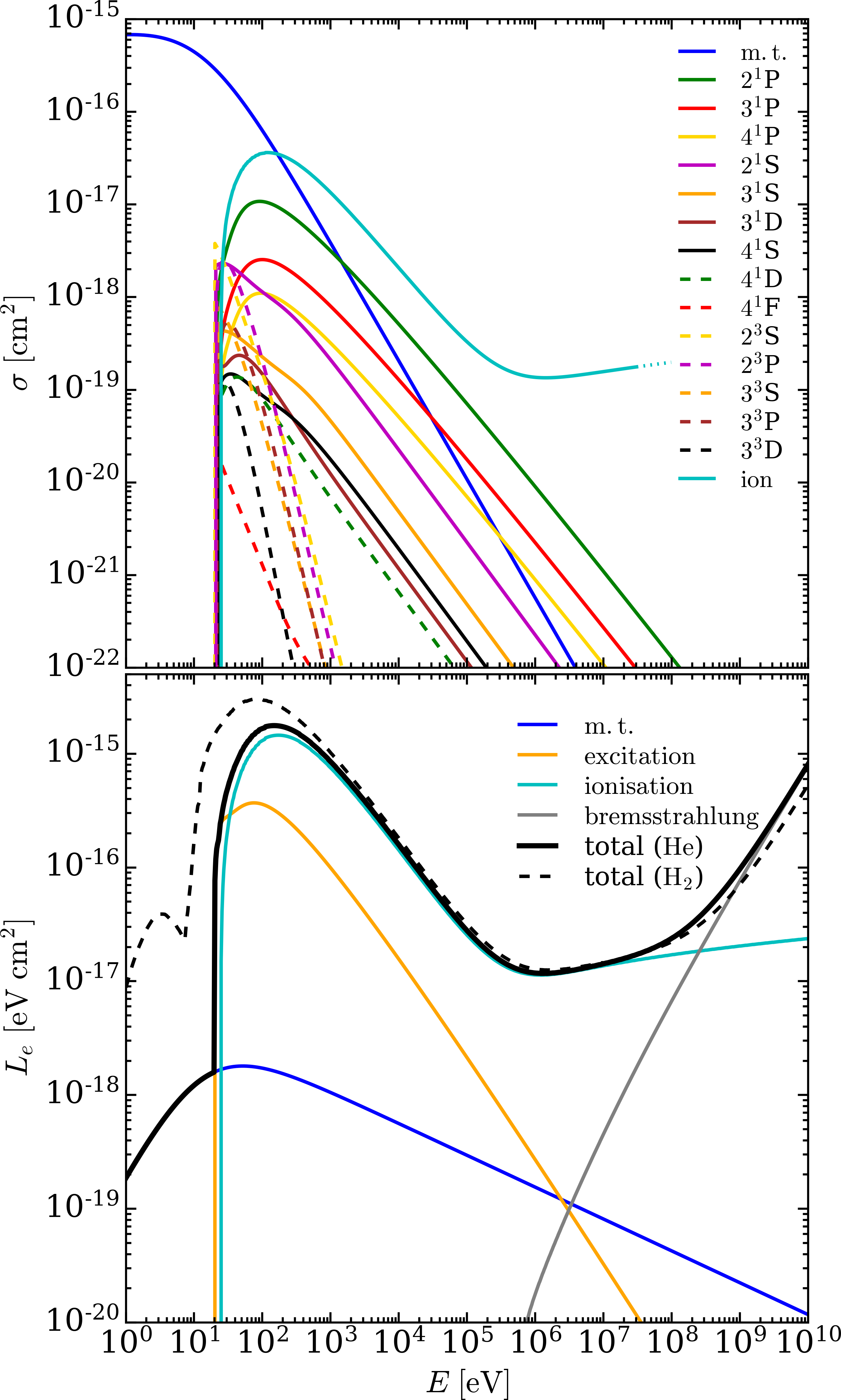
Figure 9: Upper panel: momentum transfer cross section (“m.t.”; Pinto & Galli 2008), excitation cross sections (Ralchenko et al. 2008), and ionisation cross section (“ion”; Kim et al. 2000) for electrons colliding with He atoms. Lower panel: energy loss function for electrons colliding with He (solid black line); momentum transfer loss (“m.t.”; solid blue line), total excitation loss (solid orange line), ionisation loss (solid cyan line), and bremsstrahlung loss (solid grey line, from Blumenthal & Gould 1970). For comparison, the loss function for electrons colliding with H₂ (dashed black line) is shown.

Appendix B Differential contribution to the cosmic-ray ionisation rate

In order to understand why the spectra of secondaries have a different attenuation with column density depending on the primary spectrum, it is useful to introduce the differential contribution to the ionisation rate per logarithmic energy interval, $E{\rm d}\zeta_{{\rm ion},k}/{\rm d}E$, where $k$ is the CR species. This quantity gives an indication of the energy from which the bulk of the ionisation is generated (see also Padovani et al. 2009). Solid circles in Fig. 10, which are also displayed at the same energies in the lower left panel of Fig. 4, show the primary CR energies that contribute most to the CR ionisation rate. Accordingly, solid diamonds in the right panel of Fig. 10 refer to secondary electron energies (see also the lower right panel in Fig. 4). These energies correspond to the maxima of $E{\rm d}\zeta_{{\rm ion},k}/{\rm d}E$. Looking at the left panel of Fig. 10, we see that for model $\mathscr{L}$ the peak of $E{\rm d}\zeta_{{\rm ion},p}/{\rm d}E$ is essentially independent of column density, and its maximum is at $E\simeq 100$ MeV. Conversely, for model $\mathscr{H}$, the peak of $E{\rm d}\zeta_{{\rm ion},p}/{\rm d}E$ decreases by more than one order of magnitude for H₂ column densities from $10^{20}$ cm^-2 to $10^{23}$ cm^-2, and its maximum shifts from $E\simeq 1$ MeV to $\simeq 40$ MeV. This is because model $\mathscr{H}$ has a non-negligible component of protons at low energies, which contribute to the CR ionisation rate. However, for increasing column densities, this low-energy tail is quickly attenuated (Padovani et al. 2018b), and thus the peak of $E{\rm d}\zeta_{{\rm ion},p}/{\rm d}E$ moves towards higher energies. In contrast, for model $\mathscr{L}$, the largest contribution comes from the 100 MeV protons. Such protons are only attenuated at $N_{\rm H_{2}}\gtrsim 10^{24}$ cm^-2, namely at column densities outside the range of our interest. As a result, the secondary electron spectrum from the proton model $\mathscr{L}$ is nearly independent of column density, while the spectrum from model $\mathscr{H}$ is attenuated at higher column densities. This is the reason why $\zeta_{{\rm exc},u}$ and $\zeta_{\rm ion}$ for model $\mathscr{L}$ show a weak dependence on $N_{\rm H_{2}}$, whereas for model $\mathscr{H}$ the dependence is strong (see Fig. 5). The same reasoning applies to the spectrum of primary electrons for which $E{\rm d}\zeta_{{\rm ion},e}/{\rm d}E$ decreases by more than one order of magnitude for H₂ column densities from $10^{20}$ cm^-2 to $10^{23}$ cm^-2, and its maximum shifts from $E\simeq 10$ keV to $\simeq 10$ MeV.

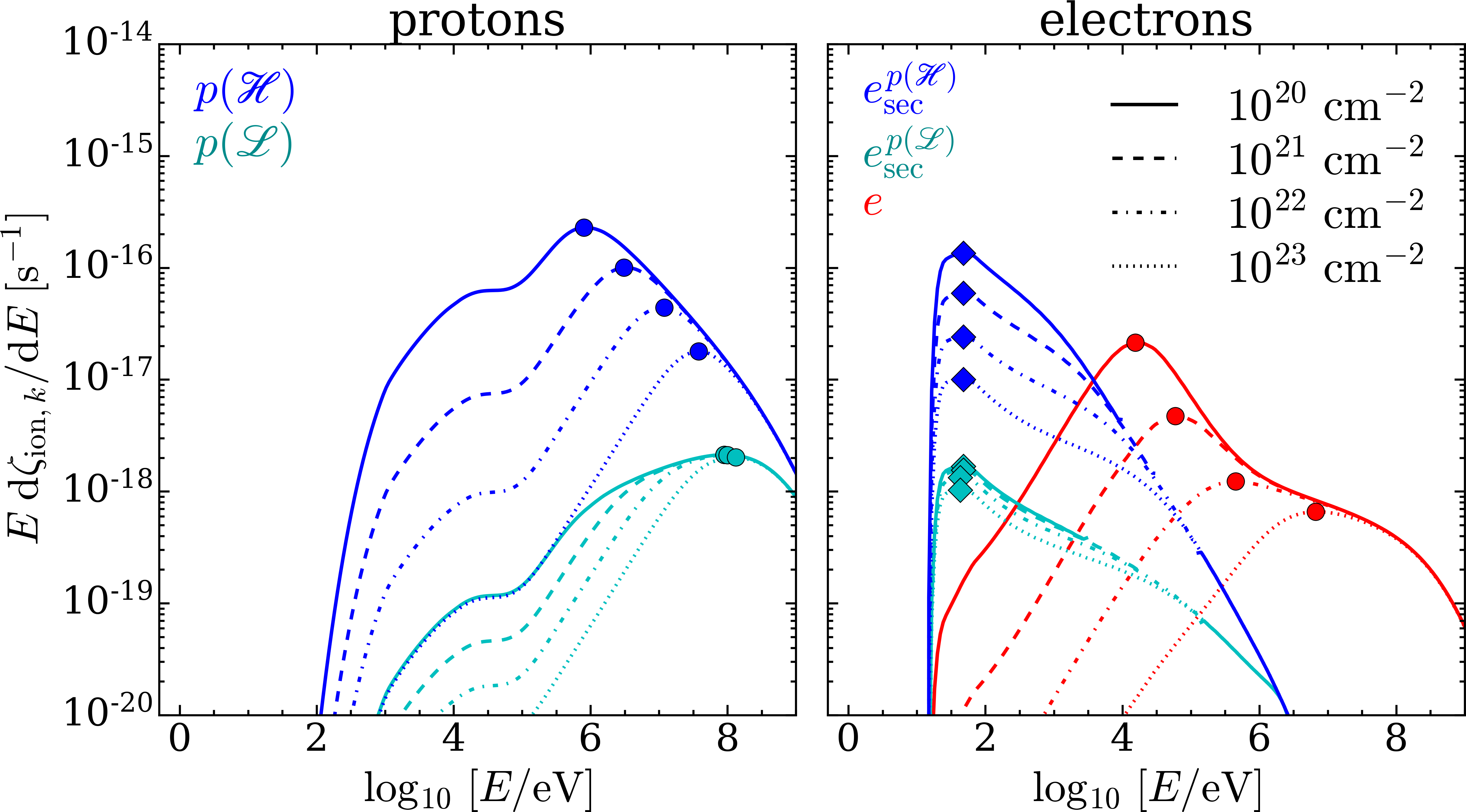
Figure 10: Differential contribution to the ionisation rate, $E{\rm d}\zeta_{{\rm ion},k}/{\rm d}E$, per logarithmic energy interval as a function of the energy at the column densities $N_{\rm H_{2}}=10^{20}$, $10^{21}$, $10^{22}$, and $10^{23}$ cm^-2. Left plot: CR protons (model $\mathscr{L}$ and $\mathscr{H}$; cyan and blue lines, respectively); right plot: CR primary electrons (red lines) and secondary electrons (model $\mathscr{L}$ and $\mathscr{H}$; cyan and blue lines, respectively). Solid circles (diamonds) denote the energies of primary CRs (secondary electrons) that contribute most to the CR ionisation rate.

Appendix C Cosmic-ray ionisation rate estimates: update from observations

In Fig. 11 we present the estimates of the CR ionisation rate obtained from observations in diffuse clouds, low- and high-mass star-forming regions, circumstellar discs, and massive hot cores. In the same plot we show the trend of $\zeta_{\rm ion}$ predicted by CR propagation models (e.g. Padovani et al. 2009, 2018b): the model $\mathscr{L}$, with low-energy spectral slope $\alpha=0.1$, which is based on the data of the two Voyager spacecrafts (Cummings et al. 2016; Stone et al. 2019); the model $\mathscr{H}$, with $\alpha=-0.8$, which reproduces the average value of $\zeta_{\rm ion}$ in diffuse regions; the model with $\alpha=-1.2$, which can be considered as an upper limit to the CR ionisation rate estimates in diffuse regions. Models also include the contribution of primary CR electrons and secondary electrons.

The spread of $\zeta_{\rm ion}$ in dense cores (Caselli et al. 1998) is supposed to be related to uncertainties in the chemical network, in the depletion process of elements such as carbon and oxygen, as well as because of the presence of tangled magnetic fields (Padovani & Galli 2011; Padovani et al. 2013; Silsbee et al. 2018). We note that the models presented here only account for the propagation of interstellar CRs, but in more evolved sources, such as in high-mass star-forming regions and hot cores, there could be a substantial contribution from locally accelerated charged particles (Padovani et al. 2015, 2016; Gaches & Offner 2018; Padovani et al. 2021b).

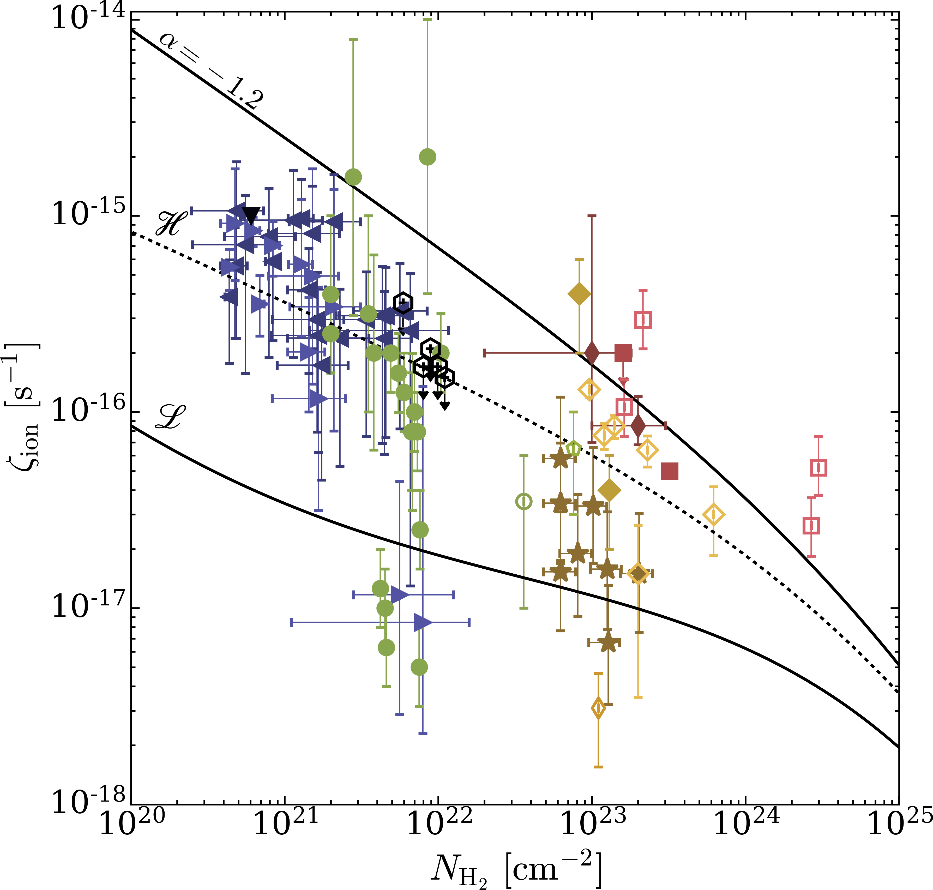
Figure 11: Total CR ionisation rate as a function of the H₂ column density. Theoretical models $\mathscr{L}$ (solid black line), $\mathscr{H}$ (dotted black line), and with low-energy spectral slope $\alpha=-1.2$ (solid black line). Expected values from models also include the ionisation due to primary CR electrons and secondary electrons. Observational estimates in diffuse clouds: down-pointing triangle (Shaw et al. 2008), left-pointing triangles (Indriolo & McCall 2012), right-pointing triangles (Neufeld & Wolfire 2017); in low-mass dense cores: solid circles (Caselli et al. 1998), empty hexagons (Bialy et al. 2021), empty circle (Maret & Bergin 2007), empty pentagon (Fuente et al. 2016); in high-mass star-forming regions: stars (Sabatini et al. 2020), solid diamonds (de Boisanger et al. 1996), empty diamonds (van der Tak et al. 2000), empty thin diamonds (Hezareh et al. 2008), solid thin diamonds (Morales Ortiz et al. 2014); in circumstellar discs: solid squares (Ceccarelli et al. 2004); in massive hot cores: empty squares (Barger & Garrod 2020).