Dealing with elementary paths in the Kidney Exchange Problem

Abstract

We study an elementary path problem which appears in the pricing step of a column generation scheme solving the kidney exchange problem. The latter aims at finding exchanges of donations in a pool of patients and donors of kidney transplantations. Informally, the problem is to determine a set of cycles and chains of limited length maximizing a medical benefit in a directed graph. The cycle formulation, a large-scale model of the problem restricted to cycles of donation, is efficiently solved via branch-and-price. When including chains of donation however, the pricing subproblem becomes NP-hard. This article proposes a new complete column generation scheme that takes into account these chains initiated by altruistic donors. The development of non-exact dynamic approaches for the pricing problem, the NG-route relaxation and the color coding heuristic, leads to an efficient column generation process.

1 Introduction

The kidney exchange problem models the barter market of kidney exchange programs, which were created to match patients waiting for a kidney transplant to living donors with the objective to find the best possible transplants to perform. Each participating patient is paired with a willing, but incompatible, donor. This donor accepts to give one kidney only if its associated patient receives one, creating cycles of donation (see Figure 1(a)). It is imperative that a patient is transplanted if its associated donor gives a kidney, so no donors should give before another and all the surgeries of a cycle must be done simultaneously. As a cycle requires twice its size operating teams and rooms, kidney exchange programs impose a limit $K$ on the size of a cycle. In a lot of countries, programs also include altruistic donors. These donors are not expecting any transplant to happen in return, creating chains of donation (or domino chains, see Figure 1(b)). In this case, the simultaneity may not be required, as no donor would give his kidney before its patient receives another one. Yet, the failure of a transplant causes the failure of every remaining transplant in the chain. Thus, it is preferable to have several shorter chains than a big one and a lot of programs impose a limit $L$ (usually $L>K$) on the length of a chain. An exchange in a kidney exchange program is therefore either a cycle or a chain of donation which implies at most $K$ (resp. $L$) transplants. The kidney exchange problem (KEP) aims at finding the best set of exchanges in order to maximize the medical benefit of the performed transplants.

(a) Cycle of donation with 3 pairs

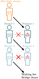
(b) Chain of donation

Figure 1: Standard exchanges in a kidney exchange program. Chains and cycles may include more pairs.

The idea of kidney exchange was first mentioned by Rapaport in 1986 [32] and quickly set up in South Korea in 1991 [23, 27]. This idea was promising for this country where the public opinion is hostile on deceased transplantation. The Switzerland was the first European country to perform a kidney exchange in 1999, but the first national kidney exchange program (KPD) in Europe was created by the Netherlands in 2004 [9]. Since then, a dozen states in Europe have created their own KPD [5]. In the rest of the world, and to the best of our knowledge, such programs exist only in Canada, Australia and the USA. We refer the reader to the survey of Ellison [12] for more details on the development of KPDs. It is worth to note that kidney exchange programs involve more and more participants as the usage is spreading in hospitals, but also due to transnational exchanges. The bigger the pool, the higher the chance to match patients, but the harder the kidney exchange problem. In 2019, the largest program in Europe involves 250 British patients [6], but considering that more than half a million Europeans [22] and even more USA citizens [35, 36] are treated for end stage kidney disease, new efficient techniques must be developed to handle many more candidates for kidney exchange programs.

Different approaches exist to solve the kidney exchange problem. When it contains only cycles of length 2, the KEP can be solved polynomially as a matching problem via Edmonds’ algorithm, but as soon as $K>2$, the problem is proved to be NP-complete [1, 7]. Consequently, the KEP is often tackled with integer programs and the major ones are surveyed by Mak-Hau [24].

We focus on the cycle formulation. The original version of this formulation does not take into account altruistic donors and requires to compute every possible cycles. Abraham et al. developed a column generation approach to solve this integer program [1], which is still to this day the best way to solve the KEP without chains of donation. The cycle formulation can be equivalently applied when including these chains, and we will refer to it as the exchange formulation. In Chen et al., all exchanges are computed beforehand [8], but this is not a viable method when the patients pool grows. On the basis of Abraham et al. work, branch-and-price algorithms were developed [16, 17, 20, 30] claiming to accommodate well altruistic donors via chains of donation. However some of these algorithms (in [16, 17, 30]) were proven wrong by Plaut et al. [31] and Klimentova et al. did not test their algorithm with altruistic donors [20]. Actually, Plaut et al. proved in 2016 that the pricing algorithm becomes NP-complete in this case.

In order to handle large-scale instances of the KEP, our objective is to address this NP-hard problem and establish efficient pricing strategies. We study its optimization version, that we refer to as the elementary minimum path problem with length constraint (EMPPLC). Based on a review of similar problems, we propose to generate lower and upper bounds using dynamic programming. This approach allows an efficient column generation process and thus to compute the linear relaxation of the exchange formulation. This upper bound on the optimal value can be used to assess the quality of the feasible solution that our algorithm constructs by solving the exchange formulation on generated columns. Our method turns out to be very efficient as the gap between lower and upper bounds is always smaller than 0.5%, even on instances with more than 800 vertices. The number of patients of these instances is larger than in the current literature or in the field, but is likely to be prevalent in a near future.

In Section 2 we model the kidney exchange problem with the exchange formulation. Section 3 defines the elementary minimum path problem with length constraint and reviews the different approaches used to solve it, in particular the key idea of our contributions. We detail in Sections 4 and 5 the improvements we developed on the NG-route relaxation and the color coding. Their performance are compared in Section 6. Finally Section 7 shows how these algorithms are used to solve the kidney exchange problem. Note that the path problem studied in this article may be found in other applications and the contributions presented here used in these other cases as well.

2 Using an exponential formulation for the KEP

We model a kidney exchange program as a directed graph by creating one vertex for each participant and one arc for each possible transplant. Formally, the set $P$ contains one vertex for each patient-donor pairs and the set $N$ one vertex for each altruistic donor. To construct the compatibility graph ${D=(V=P\cup N,A)}$, we add an arc $a={(uv)}$ between ${u\in V}$ and ${v\in P}$ if the kidney of donor $u$ can be transplanted to patient $v$. A weight function ${w:A\rightarrow\mathbb{R}^{+}}$ represents the medical benefit of each possible transplant. Note that determining the weight function is an upstream work and that $w$ is an input in our case. This graph is generally quite sparse as it is rare for a patient and a donor to be compatible. Figure 2(a) shows an example of compatibility graph and differentiates altruistic donors (orange diamonds) from pairs (red circles).

An exchange is a subgraph of $D$ which represents either a cycle of donation between pairs or a domino chain initiated by altruistic donors. In the compatibility graph, exchanges are elementary cycles of length at most $K$, called valid cycles and elementary paths starting by a vertex of $N$ and having at most $L$ vertices, valid paths. A valid cycle could have several symmetrical representations but they are eliminated by restricting the first vertex of the cycle vector to have the lowest identifier. Thus, a valid cycle $c$ is represented by a unique vector of vertices $(v_{1},...,v_{|c|})$ such that ${v_{1}<v_{j}\ \forall j\in\{2,...,|c|\}}$.

$\mathcal{C}$ is the set of all valid cycles, $\mathcal{P}$ the set of all valid paths and $\mathcal{E}=\mathcal{C}\cup\mathcal{P}$ the set of all possible exchanges. We refer to the set of vertices (resp. edges) of an exchange $e$ as $V(e)$ (resp. $A(e)$). The weight of an exchange $e\in\mathcal{E}$ is $w(e):=\sum\limits_{a\in A(e)}w_{a}$. In Figure 2(a) for example, by taking $K=3$ and $L=4$, there exists 8 exchanges: two cycles ($e_{1}=5-7-6$; $e_{2}=4-6$) and six paths ($e_{3}=1-3$; $e_{4}=1-3-5$; $e_{5}=1-3-5-7$; $e_{6}=2-3$; $e_{7}=2-3-5$; $e_{8}=2-3-5-7$).

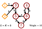
(a) Model

(b) Solution of the KEP

Figure 2: Example of a compatibility graph of a kidney exchange program

Formally, the kidney exchange problem is a maximum-weight set packing problem, where the considered sets are the exchanges. As each agent can give or receive at most one kidney, the exchanges must indeed be pairwise disjoint. Figure 2 shows the optimal solution of the KEP in our example. In the exchange formulation (EF), each exchange is associated with one binary variable indicating if it is chosen or not in the solution and a unique set of constraints (2) is required to model the disjonction of exchanges:

${\forall e\in\mathcal{E},\ x_{e}=\left\{\begin{aligned} &1\text{ if exchange $e$ is chosen }\\ &0\text{ otherwise}\end{aligned}\right.}$

$$\quad z^{*}=\max\sum\limits_{e\in\mathcal{E}}w_{e}x_{e}$$ (1)

$$\sum_{\begin{subarray}{c}e\in\mathcal{E}:\\ i\in V(e)\end{subarray}}x_{e} \leq 1 \ \forall i\in V$$ (2)

$$x_{e} \in\{0,1\} \forall e\in\mathcal{E}$$ (3)

The number of variables of EF grows exponentially with $K$ and $L$, so even computing its linear relaxation $z^{*}_{LP}$ may need an excessive amount of time or be impossible due to memory issues. However, the quality of its linear relaxation makes EF very promising. It is actually, up to now, the tightest formulation for the KEP, including compact and other large-scale formulations [11, 24]. Moreover, these other integer programs are more complex and also suffer from scalability issues.

To overcome the exponential growth of EF, its linear relaxation EF can be solved by a column generation approach. It constructs iteratively a (small) set of variables guaranteeing that an optimal solution uses only these variables with the following two steps:

1. Solve the restricted master problem (RMP): EFL restricted on a subset $\mathcal{E}^{\prime}\subseteq\mathcal{E}$.

2. Solve the pricing problem: find an “interesting” exchange to add in $\mathcal{E}^{\prime}$ (go to 1.) or prove none exists (end).

When the restricted master problem is solved, it computes for each vertex $v$ the dual values $\alpha_{v}$ associated with constraints (2). The pricing problem of the exchange formulation aims at finding a new exchange with a positive reduced cost or proving that none exists. The reduced cost of an exchange $e$ is given by ${rc_{e}=w_{e}-\sum\limits_{v\in V(e)}\alpha_{v}}$. For a non-basis variable, it estimates the improvement of the objective function if a solution includes $e$, i.e., $x_{e}>0$. It is important to note that these reduced costs are in $\mathbb{R}$ and thus can be positive or negative. As there are two kinds of exchanges, we can decompose this pricing problem into two subproblems:

• The cycle pricing problem: find a cycle of length at most $K$ of positive reduced cost, or prove none exists.

• The path pricing problem: find an elementary path of length at most $L$ starting by an altruistic donor and with a positive reduced cost, or prove none exists.

The cycle pricing problem can be solved in polynomial time with a Bellman-Ford algorithm. On the contrary, the path pricing problem is NP-complete and the proof, based on a reduction from the directed Hamiltonian path problem, was recently given by Plaut et al. [31]. We handle this decision problem with algorithms solving the associated optimization problem: the elementary minimum path problem with length constraint (EMPPLC). This article is dedicated to this problem and how to solve it.

3 Finding elementary paths

The elementary minimum path problem with length constraint belongs to the well-known family of paths problems. It is a special case of the elementary shortest path problem with resource constraints. However its specificity—the length constraint—can be exploited to strengthen existing algorithms.

3.1 Description of the problem

Let $G=(V,A)$ be a digraph such that the set of vertices $V$ includes a source $s$. Each arc $(ij)\in A$ has a cost $c_{ij}$. Let $L$ be the limit on the length (number of arcs) of a path. An $(l,i)$-path ${p=(s,i_{1},...,i_{l}=i)}$ is an elementary path of length $l$ starting from the source $s$ and ending in $i$. We denote by $A(p)$ (resp. $V(p)$) the set of arcs (resp. vertices) of $p$ and by ${c_{p}=\sum\limits_{(ij)\in A(p)}c_{ij}}$ its cost. The objective of the elementary minimum path problem with length constraint (EMPPLC) is to find $p^{*}$ an elementary $(l,i)$-path of minimum cost $c^{*}$ such that $l\leq L$.

3.2 EMPPLC in the KEP

To cast the pricing problem of the exchange formulation as a minimization problem, we consider a new weight function $c$ associating with each arc the opposite of its estimated reduced cost: ${\forall(uv)\in A,c_{uv}=-w_{uv}+\alpha_{v}}$. We also construct a new directed graph containing an artificial source $s$ linked to each altruistic donor ${D^{\prime}=(V\cup\{s\},A^{\prime})}$ where ${A^{\prime}=A\cup\{(su)\ \forall u\in N\}}$. The function $c$ is extended to these new arcs: ${\forall u\in N,c_{sv}=\alpha_{v}}$. A valid path contains $L+1$ vertices (including the source) and $L$ arcs in $D^{\prime}$. For an exchange $e$, ${c_{e}=\sum\limits_{(uv)\in A^{\prime}(e)}c_{uv}=\sum\limits_{v\in V(e)}\alpha_{v}-w_{e}=-rc_{e}}$. As ${c_{e}=-rc_{e}}$, the pricing problem aims at finding paths of negative weight or prove none exists. Thus, solving EMPPLC on $D^{\prime}$ provides an answer for both cases.

3.3 Standard approaches

Interest for elementary shortest path problems mainly arose from vehicle routing applications solved by column generation. The elementarity constraint is often relaxed to get a simpler problem, which can be relevant in many applications such as vehicle routing problems where a vehicle can visit the same place twice. In the standard case, one just wants to solve the shortest path problem (SPP), which can be done with a Bellman-Ford algorithm. In the presence of resource constraints, such as time windows or vehicle capacities, the problem becomes harder. In 1988, Desrochers [10] proposed an extension of the Bellman-Ford algorithm for the shortest path problem with resource constraints (SPPRC). However, Feillet et al. [13] argued that relaxing the elementarity constraint can lead to bounds of poor quality, thus proposed to extend Desrochers’ algorithm in order to solve the NP-hard elementary shortest path problem with resource constraints (ESPPRC). In the ESPPRC, paths have limited resources (instead of having a maximum length as in EMPPLC). Let $R$ be the number of resource types and ${g_{ij}^{r}\geq 0}$ the consumption of resource $r$ along the arc $(ij)$. Each vertex $i\in V$ constrains the path to reach it with a resource consumption belonging to ${\left[a_{i}^{r},b_{i}^{r}\right]}$ for each resource $r$. The objective is to find a path of minimum cost $c$ such that every resource constraint is satisfied. By considering a single resource with a unit consumption and by setting the bound on this resource consumption to the length limit, ESPPRC describes EMPPLC. Formally let $R=1$ and, ${\forall i\in V:}$ ${a_{i}=0}$ and ${b_{i}=L}$. In addition we set ${g_{ij}=1}$, ${\forall(ij)\in A}$ and observe that EMPPLC is a special case of ESPPRC.

When dealing with the EMPPLC, like for any problem, the objective is generally to find the optimal solution. Exact algorithms are designed for this, but as EMPPLC is NP-hard, they might take a long time to get it. On the other hand, in a column generation framework it is not important to find optimal solutions, but to find a solution with the same sign as the optimal solution. Indeed, assume the pricing problem is to find a path with a negative cost. Then any feasible solution of EMPPLC is a new column to add to the restricted master problem. Similarly, if a lower bound has a positive (or zero) cost, the optimality proof of the linear relaxation is done. Lower bounds and feasible solutions can be computed with relaxations and heuristics respectively.

Numerous approaches solving paths problems, including Desrochers’ and Feillet’, are based on dynamic programing and labeling algorithms following Held and Karp results [18]. This dynamic program solving the EMPPLC has a space complexity of $\mathcal{O}(|V|2^{|V|})$, a time complexity of $\mathcal{O}(|A|2^{|V|})$ and does not scale up to large instances. A common idea to overcome scaling issues is to relax the problem in order to deal with a smaller search space. Relaxing a minimization problem aims at quickly providing lower bounds. If we relax the constraint of elementarity, the search space is strongly reduced since the visited vertices are not remembered anymore. We can also relax the resource constraints to solve the shorstest path problem. More complex dynamic programs relax only partially these constraints. This is the case of the NG-route relaxation proposed by Baldacci et al. [4] which constructs partially elementary paths. We present their algorithm and how we reinforce it for our problem in Section 5. Note that in the kidney exchange context, the elementarity constraint cannot be relaxed to get a feasible solution, but it can be relaxed in the RMP, “temporarily”, in order to speed up the column generation. Actually, compatibility graphs are generally sparse, unlike graphs of vehicle routing problems which are usually complete, and relaxed solutions may be elementary anyway.

Another, and opposite, idea to reduce the search space in dynamic programming is to restrict the problem. More constrained problems will provide feasible solutions and thus upper bounds on the EMPPLC optimal solution. We introduce the color coding algorithm proposed by Alon et al. [3] and present our contributions in Section 4.

These two dynamic programs, the color coding and the NG-route, are the core of our study of the EMPPLC. They provide a different type of solution and to assess their interest, we compare them to two alternative algorithms that serve as baseline methods.

Firstly, we adapt an integer linear programming formulation of the traveling salesman problem called the time-stage formulation (TSF), which was proposed by Fox, Gavish and Graves [14] for the traveling salesman problem. In this model, a decision variable $y^{l}_{ij}$ states if arc $(ij)$ is taken at the $l^{\text{th}}$ position of the path. The integer program TSF is used to compute the optimal solutions of the different EMPPLC instances. It is also solved within a time limit of 1 second, giving the best lower and upper bounds TSF-lb and TSF-ub

Secondly, we develop a quick heuristic based on local search: the algorithm moves from the current solution $p$ to a better solution $p^{\prime}$ in its neighborhood. This solution $p^{\prime}$ is constructed by inserting, removing or exchanging up to 3 vertices in $p$ (see figure 3) and kept if $c_{p^{\prime}}<c_{p}$. The solution with the minimum cost is returned after one second (solution LM), as well as the first path of negative cost (solution LF). If no path of negative cost is found in the time limit, then LF is equal to LM.

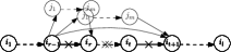
(a) Initial path

(b) Insertion

(c) Suppression

(d) Exchange

Figure 3: Movements of the local search.
Dashed arrows represent subpaths, plain arrows are edges and crossed arrows are removed in the movement.

3.4 Exploit the length constraint

As we look for a path of length at most $L$, we can use this information to reinforce shortest path algorithms. We compute with Floyd-Warshall algorithm the distance function ${d:V\times V\rightarrow\mathbb{N}\cup\{+\infty\}}$ where $d(i,j)$ is the shortest path between $i$ and $j$, with respect to the number of arcs. We define the extended neighborhood ${{\color[rgb]{0,0,0}\gamma(i)}}$ of vertex $i$ as the set of vertices that may appear in any path starting at the source of length at most $L$ including $i$: ${\gamma(i):=\{j\in V:d(s,i)+d(i,j)\leq L\text{ or }d(s,j)+d(j,i)\leq L\}}$. Note that if ${i\in\gamma(j)}$ then ${j\in\gamma(i)}$. We define the extended predecessors ${{\color[rgb]{0,0,0}\gamma^{-}(i)}}$ of vertex $i$ as the sets of vertices that can reach $i$ in a path of length at most $L$: ${\gamma^{-}(i):=\{j\in V:d(s,j)+d(j,i)\leq L\}}$.

The distance function is used first to perform a preprocessing on the graph $G$ by removing every arc (and vertex) that is too far from the source to be contained in a path of length $L$. The sets of extended neighbors and predecessors also take part in the improvements of the next sections.

4 The color coding restriction

The randomized algorithm referred to as the color coding was introduced by Alon et al. [3] to solve the subgraph isomorphism problem. It can be applied in particular to solve the elementary minimum path problem with length constraint. Its principle is to randomly assign a color to each vertex, then to solve a dynamic program finding the path of minimum weight whose vertices all have different colors. Such a path is said to be colorful and searching for it is computationally more efficient than the search for an elementary path as there are $C$ distinct vertex identifiers instead of $|V|$. However, this colorful path is not optimal in general. Indeed, for an optimal solution to be found with color coding, the random coloring must, by chance, assign different colors to its vertices. Thus, the two steps of the algorithm are repeated so that each solving of the dynamic program might return a different path, increasing the probability that one of them is optimal.

In all its applications and theoretical studies, the coloring step is performed with a discrete uniform distribution. Only Kneis et al. [21] proposed another probability distribution to color the graph, but for a derandomization purpose. We introduce in this section new strategies for this step of the algorithm and focus on how this strategies are helpful to efficiently solve the EMPPLC for our pricing step. We refer the reader to Pansart et al. [25] for the theoretical study of these new strategies in the general context of subgraph isomorphism problem, but also for an extensive literature review on color coding and proofs of properties mentioned in the following.

4.1 Description of the algorithm

To solve the elementary minimum path problem with length constraint in a weighted graph $G=(V,A)$, the color coding uses two steps:

1. Coloring: randomly assign a color $c\in\{1,...,C\}$ to each vertex $v\in V\setminus\{s\}$

2. Dynamic programming: finds the colorful path of minimum weight, of length at most $L$, whose vertices all have distinct colors. $f^{*}(\mathcal{C},i)$ is the minimal cost of a path from $s$ to $i$, using $|\mathcal{C}|-1$ arcs and visiting vertices of each color of $\mathcal{C}$:

   $$f^{*}(\mathcal{C},i)=\min\limits_{\begin{subarray}{c}j\in N^{-}(i)\\ c_{j}\in\mathcal{C}\setminus\{c_{i}\}\end{subarray}}\{f^{*}(\mathcal{C}\setminus\{c_{i}\},j)+c_{ji}\}$$ (4)

These two steps are repeated several times in order to guarantee a probability high enough that one of these trials finds an optimal path. In the standard version of the color coding, the coloring step applies a discrete uniform distribution to assign the colors and $C=L$. In this case, the number of trials required to ensure that a specific path (e.g., an optimal path) of length $L$ is colorful with probability $\rho$ is ${t=\frac{ln(1-\rho)}{ln(1-\frac{C!}{C^{C}})}}$.

Using more colors can however increase the chance for a path to be colorful, thus reduce the number of trials $t$, but it also increases the complexity of the dynamic programming step. Hüffner et al. [19] analyzed the best trade-off between these two parameters: the number of trials and the runtime of one trial. Another lever on the color coding efficiency is the probability distribution used to color the graph. Surprisingly though, the coloring strategy always follows the discrete uniform distribution, except in Kneis et al. [21] for a derandomization purpose. With this strategy, assigning a color to a vertex does not depend on other vertices colors. Yet, using a different probability distribution can significantly increase the probability that an optimal path is colorful, and, contrarily to increasing $C$, will not affect the computational performance of the dynamic program. The new method we introduce in the next section is based on this idea.

4.2 New randomized strategies

We propose to use a coloring technique that aims at spreading the colors in extended neighborhoods. To do so, it tries to make extended neighborhoods colorful by relying on three main ideas. First, a preprocessing step applies a local search to create an ordering of vertices $x_{1},...x_{n}$ ($x_{i}\in V$) in which extended neighbors are gathered. Secondly, the vertices are colored by intervals of size $C$ such that each interval is colorful. The color assigned to a vertex therefore depends on the color of other vertices in this interval. Finally, the ordering is shifted so that the intervals are made up of different extended neighbors each iteration.

The preprocessing step constructs a coloring sequence with the objective to gather in this sequence vertices that might belong to a solution. Such vertices are identified thanks to the extended neighborhoods. Let $x_{i}$ be the position of vertex $i$ in the sequence and $\delta$ be the sum of differences between the positions of two extended neighbors: ${\delta=\sum\limits_{\begin{subarray}{c}i\in V\\ j\in\gamma(i)\end{subarray}}|x_{i}-x_{j}|}$. Our preprocessing constructs a coloring sequence such that $\delta$ is minimized, i.e., the average distance between the positions of two extended neighbors is minimized. This problem is known as the (minimum) linear arrangement problem [2] that was proven to be NP-complete [15]. We handle it with a local search and this method is referred to as la ordering.

We denote by $(x_{1},...,x_{n})$ the coloring sequence of vertices of $V\setminus\{s\}$ provided by this preprocessing step. Our coloring strategy spread splits the coloring sequence into intervals of size $C$ and colors vertices such that these intervals are colorful. Concretely, the colors vector of vertices in an interval $I$ is a permutation of $\{1,...,C\}$ drawn with a uniform distribution over all the permutations. The color of a vertex thus depends on the colors taken by other vertices of the same interval, but on no other vertex. Thus, two vertices in the same interval cannot have the same color and two vertices in different intervals are assigned the same color with probability $\frac{1}{C}$ (proof in [25]). Once the dynamic program is solved, the coloring sequence is offset by 1 to the left. So after the first trial, the coloring sequence is $(x_{2},...,x_{n},x_{1})$. This shifted-spread strategy means that, after $C$ trials of the color coding, every subsequence of size $C$ has been colorful once.

Thus, if an optimal path has been gathered enough in the coloring sequence by the preprocessing, it will be colorful and found in $C$ trials only. In general we cannot know when this happens, but it can be guaranteed by a parameter of the coloring sequence: the maximum distance between the positions of two extended neighbors ${\Delta=\max\limits_{\begin{subarray}{c}i\in V\\ j\in\gamma(i)\end{subarray}}|x_{i}-x_{j}|}$. When $\Delta\leq C$, every optimal path is contained in a subsequence of size at most $C$ and our algorithm guarantees to find them with a probability of 1 with at most $C$ trials of the color coding, so only $C$ calls to the costly dynamic program.

The worst case for this coloring strategy is to have the positions of all the vertices of every optimal path in different intervals. In this case, which should not happen often in practice thanks to the la ordering, the probability that a path is colorful is the same than when using the discrete uniform distribution (proof in [25]). Thus, the method we propose always improve the chance to find an optimal solution over the original color coding.

To sum up, our method lass (la ordering + shifted-spread) contains a preprocessing phase and a color coding phase with three steps:

1. Apply a spread coloring strategy

2. Solve the dynamic program

3. Shift the coloring sequence

When $\Delta\leq C$ these three steps are repeated only $C$ times and the solution is optimal, otherwise we limit the running time and get the best solution after one second (solution CM). We also return the first negative solution (solution CF), if applicable. This time limit is small as the elementary minimum path problem with length constraint must be solved a lot of times in a column generation scheme. On the contrary, the la ordering is a preprocessing applied only once by instance of the master problem, so we let the local search runs for 300 seconds. When applied in the pricing step to solve the kidney exchange problem, this method often returns the optimal solution, even when $\Delta>C$. Indeed, graphs are sparse so the extended neighborhoods are small enough to make the preprocessing powerful. This performance allows a quick and effective solving of the pricing problem. Yet, if the color coding does not find a path of negative cost, it does not prove that the column generation has finished since this solution is only an upper bound. Thus, another method is still required to make this proof: this is the role of the NG-route relaxation.

5 The ng-route relaxation

In 2011, Baldacci et al. [4] proposed a new relaxation of the elementary shortest path problem with resource constraints called NG-route. The memory of a path is relaxed so that the search space of the dynamic program is reduced. In practice, a path constructed in the NG-route relaxation, called an NG-path, can forget that it went through some vertices and may visit them several times and be non elementary. However, if it turns out that the NG-path is elementary, then it is an optimal solution of the ESPPRC. We describe the adaptation of this algorithm for the EMPPLC special case.

Note that solving the EMPPLC with the NG-route relaxation in a column generation scheme can lead to the introduction of non elementary columns in the RMP. In this case, the column generation does not solve the linear relaxation of the master problem, but a relaxation of this linear problem. In the KEP context, the solution obtained with non-elementary paths is thus an upper bound on $z^{*}_{L\!P}$, but it can be used similarly, for example to assess the quality of a feasible solution. Of course if only elementary paths were added by the NG-route relaxation, this upper bound is actually $z^{*}_{L\!P}$. As compatibility graphs are rather sparse, the elementarity will be often satisfied by NG-paths.

5.1 Description of the algorithm

In this relaxation, each vertex $i$ has a “memory”, also named NG-set, denoted by ${\eta_{i}\subseteq V}$ and such that ${i\in\eta_{i}}$. If an NG-path goes through $i$, it can remember only vertices of $\eta_{i}$. As it is true for each vertex, an NG-path only remembers the vertices appearing in every NG-set. An NG-path of minimum cost with respect to these NG-sets can be constructed by a dynamic program, either in a forward or backward scheme. We detail below the forward dynamic program and refer the reader to the paper of Baldacci et al. for the backward version.

Each path ${p=(s,i_{1},...,i_{l})}$ is associated with a set of remembered vertices ${\Pi(p)=\left\{i_{r}:i_{r}\in\bigcap\limits_{t=r+1}^{l}\eta_{i_{t}},r=1,...,l-1\right\}\bigcup\{i_{l}\}}$.

A forward NG-path ${(\Pi,l,i)}$, is a (non necessarily elementary) path ${p=(s,i_{1},...,i_{l}=i)}$ starting from $s$, ending in $i$, using $l$ arcs and such that ${\Pi=\Pi(p)}$. $\Pi$ represents the memory of $p$, since no vertex of $\Pi$ can be used to extend $p$. $p$ is constructed by adding $i$ to a smaller NG-path that belongs to the set ${\Psi^{-}\left(\Pi,l,i\right)}$:

$$\Psi^{-}\left(\Pi,l,i\right)=\left\{\right. (\Pi^{\prime},l-1,j)\text{ ng-paths s.t.}:$$

$$j\in N^{-}(i),\Pi=\left(\Pi^{\prime}\cap\eta_{i}\right)\cup\{i\},\Pi^{\prime}\subseteq\eta_{j},j\in\Pi^{\prime},i\notin\Pi^{\prime}\left.\right\}$$

$f^{*}(\Pi,l,i)$ is the minimal cost of an NG-path $(\Pi,l,i)$ and can be computed with the following recursive formula:

$$f^{*}(\Pi,l,i)=\min\limits_{(\Pi^{\prime},l-1,j)\in\Psi^{-}\left(\Pi,l,i\right)}\{f^{*}\left(\Pi^{\prime},l-1,j\right)+c_{ji}\}$$ (5)

5.2 Decremental State-Space Relaxation

Pecin et al. [29] proposed to use the Decremental State-Space Relaxation (DSSR) technique of Righini and Salani’s [33], an iterative algorithm in which the search space is even more relaxed than in the pure NG-route relaxation. At each iteration $k$, each vertex $i$ is associated with a set $\mu^{k}_{i}$ that takes the role of the NG-set $\eta_{i}$ in the dynamic program. At the first iteration the subsets $\mu^{0}_{i}$ are empty sets. When the solution $p_{k}$ of iteration $k$ is not elementary and does not respect the chosen criterion, vertices are added to the sets $\mu^{k}_{i}$ and a new iteration begins. There are three main possible criteria in the DSSR NG-route algorithm.

• predefined: original NG-sets $\eta_{i}$ are computed and the DSSR continues until $p_{k}$ is either elementary or a feasible NG-path with respect to these sets. Vertices are added to sets $\mu^{k}_{i}$ only if they belong to $\eta_{i}$.

• limited: the DSSR continues until $p_{k}$ is elementary or the sizes of sets $\mu^{k}_{i}$ exceed a given limit.

• unlimited: the DSSR continues until $p_{k}$ is elementary.

Without descent or with a predefined one, NG-sets are the heart of the algorithm since they determine the quality of the solution as well as the computation efficiency. When $\eta_{i}$ is empty for every vertex, there is absolutely no constraint on the elementarity of the path and the NG-route relaxation solves the SPPRC. When $\eta_{i}=V$ for every vertex, the NG-route is not a relaxation anymore and the solution is necessarily elementary. Except for the unlimited DSSR-NG-route, the NG-sets have a limited size of $\Lambda$ and, in general, they are constructed randomly. We propose to exploit the length constraint of the problem and to take into account the extended neighborhoods in the NG-sets construction. Indeed, it is sufficient for a vertex to “remember” in $\eta_{i}$ only its extended predecessors since they are the only vertices that can appear in a path reaching $i$. Moreoever, when the EMPPLC is embedded in a column generation framework, vertices are associated with a dual value which usually represents the interest for the vertex to appear in the solution. The memory of a vertex can therefore be composed by its $\Lambda$ extended neighbors with the highest dual value.

We also apply the filtering proposed by Pecin et al. [29] based on the alternation between forward and backward computations of the NG-path in a DSSR scheme. Assume we have $UB_{p}$ an upper bound on the EMPPLC optimal value. At each iteration, the costs computed in the previous iteration can be used as completion bounds. Thus, for each state of the dynamic program, a lower bound on the cost of a NG-path constructed from this state can be calculated. If this bound is greater than $UB_{p}$, then the state is pruned as it never be part of an optimal solution. A natural upper bound in our case is $0$ as we are looking for a path of a negative cost.

The solution of this relaxation can be a non elementary path. However in the context of the kidney exchange problem, graph are sparse so the elementarity is often achieved even with a relaxed memory. Moreover, the NG-route algorithm is not aimed at finding columns to add in the column generation, but rather at proving the end of the column generation. Ideally, it will be called only once at the end of the column generation and in practice the number of calls is indeed low (4.2 in our experiments) due to the efficiency of our color coding method.

6 Experiments on EMPPLC algorithms

We first detail the instances and the protocol, then we analyze the performance of the different algorithms studied in this article to solve the elementary minimum path problem with length constraint.

6.1 Instances and protocol

Experiments are conducted on several EMPPLC instances generated from the pricing step of KEP instances. Pools of patients and donors are created using an online Saidman-based generator [34] with realistic parameters, leading to sparse graphs. In this benchmark called KBR, there are 27 different classes of instances. In particular, the number of patients varies between 50 and 250, ${K=3}$ and ${L\in\{4,7,13\}}$. The exchange formulation is solved by column generation on one instance of each class and EMPPLC instances are extracted from the first, last and middle iterations of the pricing problem. Note that the 54 instances generated from the first and middle iterations (instances E-KBR^-) contain a solution of negative weight while the optimal value for the 27 last iterations (instances E-KBR⁰) is zero. The purpose of generating instances with such a procedure is to get dual values at different stages of the column generation, so different weight functions $c$.

In a column generation, methods providing feasible solutions are designed to quickly find new columns to add, i.e., find a path with a negative reduced cost. For this reason, heuristics either stop when the first solution of negative cost is found, or run within a small time limit. On the contrary, relaxations must find good solutions to allow filtering and computation of good bounds. Therefore, the NG-route relaxation is not limited in time while the color coding and local search algorithms are set to return the first solution of negative cost and the best solution after 1 second of running time. Note that the color coding actually ends after at least one trial was completely executed, so the effective running time may exceed this time limit. The integer program is used to compute the optimal solution, but also best upper and lower bounds within 1 second. All in all, seven solution types are reported:

• 5 upper bounds

  • CF: first solution of color coding

  • CM: best solution of color coding in 1 second

  • LF: first solution of local search

  • LM: best solution of local search in 1 second

  • TSF-ub: best feasible solution of the integer program in 1 second

• 2 lower bounds

  • NG: best NG-route of the instance

  • TSF-lb: best lower bound of the integer program in 1 second

The quality of a solution of cost $c$ is evaluated against the optimal value $c^{*}$ with three performance indicators: its gap to optimal (${\frac{|c-c^{*}|}{c^{*}}}$), its optimality (${c=c^{*}}$) and its sign compared to optimal solution. Since instances of E-KBR⁰ have an optimal value of 0, solutions CF and LF are not reported for these instances and the gap is not computed either.

All the experiments were performed on an Intel Xeon E5-2440 v2 @ 1.9 GHz processor and 32 GB of RAM.

6.2 Color coding

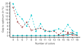
(e) $L=4$ (18 instances)

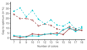
(f) $L=7$ (18 instances)

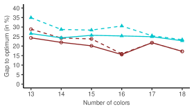
(g) $L=13$ (18 instances)

Figure 4: Gap between CF or CM and OPT depending on the configuration and the number of colors, for the E-KBR^- benchmark

We conducted experiments to determine the best number of colors and the best probability distribution to solve the EMPPLC with color coding. We observe that our method lass outperforms the standard color coding algorithm which uses a unif distribution.

Figures 4 show the gap for the E-KBR^- benchmark. The 54 instances are grouped in three sets of 18 instances, according to the parameter $L$. The first negative solution CF for the lass strategy is almost always better than for the standard color coding unif. Its quality increases with the number of colors and this is due to the fact that a trial of color coding is more efficient with more colors, both for lass and unif configurations. However, an important condition for the color coding to return good solutions is to make many trials. As increasing $C$ also increases the running time of one trial, it leads to poorer solutions in the same time limit, hence the growing gap for CM. When $C$ is too big, the color coding can exceed the time limit (see Figure 5) because an iteration runs during more than one second. In this case, the color coding actually stops after a single iteration and CF $=$ CM. From this analysis, the best compromise seems to run the color coding with a lass configuration and a small number of colors (we take ${C=L+1}$).

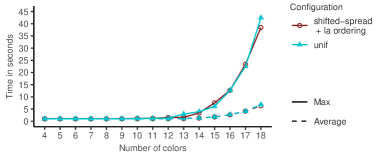
Figure 5: Average and maximum color coding running times depending on the number of colors and the configuration on E-KBR^- instances

6.3 NG-route

	NG-set creation	Descent
UN	Uniform	None
NN	Neighborhood	None
L	-	Limited
UP	Uniform	Predefined
NP	Neighborhood	Predefined

Table 1: The five versions of the NG-route relaxation

Five versions of the NG-route are implemented and tested, voluntarily omitting the unlimited DSSR as it provides no control on the computation time and memory space. Table 1 sums up the different versions and how they construct the NG-set and which DSSR is applied, if any. We tested different size limits for the NG-set (5 to 13), but it appears that they make no difference on the solution quality. On the other hand, increasing this size limit deteriorates the computation time, in particular for configurations without descent. Thus, only results for a size of 5 are kept.

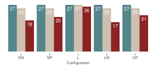
(a) Number of instances, out of 27, for which NG $=$ OPT

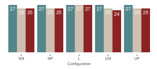
(b) Number of instances, out of 27, for which NG and OPT have the same sign

Figure 6: Quality of the NG-route solution depending on the configuration on E-KBR instances

Figures 6 illustrate the quality of the NG-route solution for the E-KBR benchmark. The 81 instances are grouped into three sets of 27 instances, according to the parameter $L$. Figure 6(a) shows the number of instances optimally solved by the NG-route relaxation, i.e., the number of instances for which the NG-route returns an elementary NG-path, so the optimal solution. Figure 6(b) shows the number of instances for which the lower bound returned by the relaxation has the same sign as the optimal solution, a success criterion for the column generation algorithm. Both figures demonstrate the good performance of the limited DSSR compared to other configurations, even though all of them are quite efficient. Still, the limited DSSR is the only configuration that always returns a solution of the same sign as the optimal one and finds this optimal solution almost every time. The fact that the solution of the NG-route is often the optimal solution explains the fact that increasing the NG-set size is not interesting, as even when they are small the solution is elementary.

6.4 Comparisons of four EMPPLC algorithms

The four algorithms were implemented and tested on the two benchmarks E-KBR^- and E-KBR⁰. Recall that for E-KBR⁰, the gap cannot be computed and that CF and LF solutions do not make sense as no feasible solutions of negative weight can be found for these instances. Thus, for this benchmark, Table 2 shows only the number of instances for which:

• the solution has the same sign as the optimal one

• the solution is the optimal one

for solutions CM, LM, TSF-ub, NG and TSF-lb.

	Upper bounds			Lower bounds
	CM	LM	TSF-ub	NG	TSF-lb
# instances with good sign	27	27	24	27	19
# instances with optimal solution	27	26	24	27	19

Table 2: Quality of solutions for the 27 E-KBR⁰ instances

	Upper bounds					Lower bounds
	CF	CM	LF	LM	TSF-ub	NG	TSF-lb
# instances with good sign	54	54	41	41	51	54	40
Average gap on such instances (%)	17.4	7.4	75.8	25.2	15.2	0.01	0
# instances with optimal solution	18	40	1	17	40	53	40

Table 3: Quality of solutions for the 54 E-KBR^- instances

Table 3 for E-KBL^- is more complete as it also displays the gap with the optimal solution for instances having a solution of the same sign as the optimal one. This gap is therefore not computed on the same number of instances for all the solutions. These results illustrate the dominance of the dynamic programs to compute both upper and lower bounds. The NG-route relaxation always finds the optimal solution, except once. No time limit was given to this algorithm, but we observe in Table 4 that it actually runs very quickly. TSF provides poorer results with the same average running time, which, besides, is bounded by the time limit. Similarly, the color coding is very powerful as it finds the optimal solution for 67 instances out of 81. Even when it does not succeed to find the optimum, the gap is the smallest among every feasible solutions. On the contrary, the local search sometimes (for 13 instances) fails to find a negative solution when there is one.

Most importantly, the color coding and the NG-route always return a solution which has the same sign as the optimal solution in a small amount of time. Thus, these algorithms are really suitable for the pricing step of a column generation scheme.

	CM∗∗	LM∗∗	TSF∗	NG
Average	1.17	1.05	0.44	0.43
Maximum	2.39	3.05	1.51	2.76

Table 4: Average and maximum running times to get solutions
^∗  Time limit of 1 second
^∗∗ Soft time limit of 1 second (checked only between iterations)

7 Solving the kidney exchange problem

In the previous sections, algorithms and results are provided for the elementary minimum path problem with length constraint. Our initial goal is however to solve the kidney exchange problem. In this section, we present experimental results comparing the performance of the previous algorithms in a column generation scheme.

7.1 Complete algorithm

Figure 7: Our algorithm solving the kidney exchange problem: CG-dyn

The complete framework of our implementation called CG-dyn is shown in Figure 7. It solves only the path pricing problem while cycles of donation are all computed beforehand and form the initial set of variables $\mathcal{E}^{\prime}$. This is more efficient when $K=3$ than solving the complete pricing problem as preliminary experiments revealed.

The path pricing problem is solved with the two dynamic programs (color coding and NG-route) studied in this article. The color coding is limited to 1 second at each iteration of the column generation. Then, if the color coding fails to find an improving path within this time limit, the NG-route relaxation is called. Recall that the KEP is a maximization problem so a path $e$ should have a positive reduced cost $rc_{e}$ to be added in the column generation. When the NG-route relaxation does not find an improving path, i.e., every reduced cost is negative or zero, then the column generation stops. If the solution of this last NG-route relaxation was elementary, thus optimal, then the linear relaxation $z^{*}_{L\!P}$ is returned. Otherwise, the last value of RMP $\bar{z}$ is only an upper bound $U\!B$ on this value. If a given time limit was reached before finishing the column generation, then we cannot conclude on the link between $z^{*}_{L\!P}$ and the current value of RMP $\bar{z}$. However, we can still compute an upper bound $U\!B$ with Lagrangian relaxation. This upper bound is computed by relaxing in the objective function the redundant constraint stating that there are at most $|V|/2$ exchanges in the compatibility graph (see [26] for more details).

After the column generation, the final integer solution $\underline{x}$ is computed with the integer program exchange formulation restricted on $\mathcal{E}^{\prime}$ as it runs very quickly, especially compared to the column generation running time. This step is not required if the last computed solution $\bar{x}$ is already integer. The NG-route relaxation is also used to filter suboptimal arcs and vertices of the kidney exchange problem instance.

These results also demonstrate that adding all the subpaths of the EMPPLC solution speeds up the column generation. Concretely, when the path ${(s,v_{1},...,v_{l})}$ is added to $\mathcal{E}^{\prime}$, we also add the paths ${(s,v_{1},...,v_{l-1})}$, ${(s,v_{1},...,v_{l-2})}$, and so on until ${(s,v_{1},v_{2})}$.

7.2 Performance of the pricing step

The efficiency of dynamic programming approaches to solve the elementary minimum path problem with length constraint was demonstrated in Section 6. To find out if this is still the case when they are embedded in a column generation scheme solving the KEP, we compared our algorithm CG-dyn with another column generation called CG-tsf, which handles the pricing step with the local search heuristic and the time-stage formulation. Every other parameter of the column generation framework is the same for both algorithms, in particular they generate all cycles in the master problem, add every subpath in $\mathcal{E}^{\prime}$, and solve a restricted exchange formulation at the end instead of solving a complete branch-and-price. They are applied on 135 instances (5 in each class of KBR), each within a time limit of 2000 seconds.

	CG-dyn	CG-tsf
# $z^{*}_{L\!P}$ computed	135	120
Average gap between UB and LB	0.13 %	3.02 %
# $z^{*}$ computed (gap = 0)	93	84

Table 5: Results for the two different CG schemes on 135 instances after 2000 seconds of running time

L	CG-dyn	CG-tsf
4	1.6	8.9
7	10	34.3
13	15.6	673.1

Table 6: Average running time (in seconds), depending on $L$, for the 120 instances solved in the time limit

Table 5 shows that our algorithm always finds the linear relaxation EFL while CG-tsf reaches the time limit for 15 instances (those with ${|P|=250}$ and ${L=13}$). Consequently, the CG-dyn algorithm finds the optimal solution of the integer program exchange formulation for more instances. For both algorithms, this integer solution is mostly found because the linear relaxation is integer (and valid), and in this case there is no need to call the integer program after the column generation. Moreover, considering the 120 instances for which both methods find the linear relaxation in 2000 seconds, the running time is significantly smaller for CG-dyn than CG-tsf (see Table 6). These results support the efficiency of the dynamic programs to solve the path pricing problem in a column generation for the KEP.

7.3 Scaling up

As kidney exchange programs are growing, we experiment CG-dyn on larger instances, generated as before but with different parameters. In particular, it seems reasonable to consider that most of the altruistic donors are already included in kidney exchange programs, unlike patients for whom such programs are very different from the standard procedure. Thus, the proportion of altruistic donors would probably be low in future large programs. In the end, we apply CG-dyn on 20 instances, divided in 4 classes (${L\in\{4,7\}}$, ${|P|\in\{500,750\}}$, ${p_{|N|}=1\%}$).

Results, summarized in Table 7, show that the quality of the solution is still very high. Every instance was solved in less than half an hour and in average rather quickly. We also tried to solve instances with ${L=13}$ or ${|P|=1000}$, but encountered memory issues. However, our implementation does not profit from the fact that instances are quite sparse, so a more efficient implementation should overcome these memory errors. Moreover, while solving the final integer program corresponds in average to less than 1% of the running time on realistic instances, for these large instances it represents more than 5%, sometimes almost 15%. It is likely that this proportion will increase with the size of instances, making necessary the development of new algorithms to find feasible solutions.

	$|P|=500$		$|P|=750$
	$L=4$	$L=7$	$L=4$	$L=7$
Average gap between UB and LB	0.05%	0.18%	0.06%	0.23%
Average running time (seconds)	5.6	123.6	23.1	1823.5

Table 7: Results of CG-dyn on 40 large instances

8 Conclusion

In this article, we designed a complete column generation framework to solve the kidney exchange problem including altruistic donors. Due to the hardness of the pricing problem in this case, an extension of previous column generation schemes containing only cycles was not possible. We therefore proposed a new framework showing excellent results on realistic instances and promising for larger instances. We believe that the memory issues encountered for instances with $|P|=1000$ can be avoided with an implementation of the column generation using algorithms and data structures adapted to large and sparse instances. For example, the preprocessing step computing the distances between each pair of vertices could be performed with a Johnson’s algorithm instead of Floyd-Warshall.

This column generation relies on the efficiency of the dynamic approaches to handle the pricing problem, referred to as the elementary minimum path problem with length constraint. This problem has to be solved many times in the column generation framework. We adapted algorithms from the literature of shortest paths problem to better fit the specificity of our problem and designed an experimental protocol to assess their quality. The development of a new method for the color coding algorithm, including a preprocessing phase ordering the vertices, a new procedure to color the graph and a shifting technique, is promising for many applications. Indeed, it guarantees to find the optimal solution in only $C$ calls to the dynamic program in some particular cases and in any case outperforms the original discrete uniform strategy. Our complete study of this method can be found in [25]. Other improvements can be considered to get even better results. In particular, an adaptation of the different techniques proposed by Pecin et al. [28], including memory cuts, would probably strengthen our implementation of the NG-route relaxation. We also intend to study the application of the color coding for other pricing problems where it is surprisingly absent, for example for vehicle routing problems.

References

- Abraham et al., [2007] Abraham, D. J., Blum, A., and Sandholm, T. (2007). Clearing algorithms for barter exchange markets: Enabling nationwide kidney exchanges. In Proceedings of the 8th ACM conference on Electronic commerce, pages 295–304. ACM.
- Adolphson and Hu, [1973] Adolphson, D. and Hu, T. C. (1973). Optimal linear ordering. SIAM Journal on Applied Mathematics, 25(3):403–423.
- Alon et al., [1995] Alon, N., Yuster, R., and Zwick, U. (1995). Color-coding. Journal of the ACM (JACM), 42(4):844–856.
- Baldacci et al., [2011] Baldacci, R., Mingozzi, A., and Roberti, R. (2011). New Route Relaxation and Pricing Strategies for the Vehicle Routing Problem. Operations Research, 59(5):1269–1283.
- Biró et al., [2017] Biró, P., Burnapp, L., Haase, B., Hemke, A., Johnson, R., van de Klundert, J., and Manlove, D. (2017). First handbook: Kidney exchange practices in Europe. Technical report, European Network for Collaboration on Kidney Exchange Programmes.
- Biró et al., [2019] Biró, P., Haase-Kromwijk, B., Andersson, T., Ásgeirsson, E. I., Baltesová, T., Boletis, I., Bolotinha, C., Bond, G., Böhmig, G., Burnapp, L., and Others (2019). Building kidney exchange programmes in Europe—an overview of exchange practice and activities. Transplantation, 103(7):1514.
- Biro et al., [2009] Biro, P., Manlove, D. F., and Rizzi, R. (2009). Maximum weight cycle packing in directed graphs, with application to kidney exchange programs. Discrete Mathematics, Algorithms and Applications, 1(04):499–517.
- Chen et al., [2011] Chen, Y., Kalbfleisch, J. D., Li, Y., Song, P. X. K., and Zhou, Y. (2011). Computerized platform for optimal organ allocations in kidney exchanges. In Proceedings of the International Conference on Bioinformatics & Computational Biology (BIOCOMP), page 1. The Steering Committee of The World Congress in Computer Science.
- De Klerk et al., [2005] De Klerk, M., Keizer, K. M., Claas, F. H. J., Witvliet, M., Haase-Kromwijk, B. J. J. M., and Weimar, W. (2005). The Dutch national living donor kidney exchange program. American Journal of Transplantation, 5(9):2302–2305.
- Desrochers, [1988] Desrochers, M. (1988). An algorithm for the shortest path problem with resource constraints. Technical Report G-88-27, GERAD, Ecole des HEC, Canada.
- Dickerson et al., [2016] Dickerson, J. P., Manlove, D. F., Plaut, B., Sandholm, T., and Trimble, J. (2016). Position-indexed formulations for kidney exchange. In Proceedings of the 2016 ACM Conference on Economics and Computation, pages 25–42. ACM.
- Ellison, [2014] Ellison, B. (2014). A systematic review of kidney paired donation: Applying lessons from historic and contemporary case studies to improve the US model. Technical report, The Wharton School of the University of Pennsylvania.
- Feillet et al., [2004] Feillet, D., Dejax, P., Gendreau, M., and Gueguen, C. (2004). An Exact Algorithm for the Elementary Shortest Path Problem with Resource Constraints: application to some Vehicle and Routing Problems. Networks: An International Journal, 44(3):216–229.
- Fox et al., [1980] Fox, K. R., Gavish, B., and Graves, S. C. (1980). An n-constraint formulation of the (time-dependent) traveling salesman problem. Operations Research, 28(4):1018–1021.
- Garey et al., [1974] Garey, M. R., Johnson, D. S., and Stockmeyer, L. (1974). Some simplified NP-complete problems. In Proceedings of the sixth annual ACM symposium on Theory of computing, pages 47–63. ACM.
- Glorie et al., [2012] Glorie, K., Wagelmans, A., and van de Klundert, J. (2012). Iterative branch-and-price for large multi-criteria kidney exchange. Technical report, Econometric institute, Erasmus University Rotterdam.
- Glorie et al., [2014] Glorie, K. M., van de Klundert, J. J., and Wagelmans, A. P. M. (2014). Kidney exchange with long chains: An efficient pricing algorithm for clearing barter exchanges with branch-and-price. Manufacturing & Service Operations Management, 16(4):498–512.
- Held and Karp, [1962] Held, M. and Karp, R. M. (1962). A dynamic programming approach to sequencing problems. Journal of the Society for Industrial and Applied Mathematics, 10(1):196–210.
- Hüffner et al., [2008] Hüffner, F., Wernicke, S., and Zichner, T. (2008). Algorithm engineering for color-coding with applications to signaling pathway detection. Algorithmica, 52(2):114–132.
- Klimentova et al., [2014] Klimentova, X., Alvelos, F., and Viana, A. (2014). A new branch-and-price approach for the kidney exchange problem. In International Conference on Computational Science and Its Applications, pages 237–252. Springer.
- Kneis et al., [2011] Kneis, J., Langer, A., and Rossmanith, P. (2011). Derandomizing Non-uniform Color-Coding I. Technical report, RWTH Aachen - Department of Computer Science.
- Kramer et al., [2019] Kramer, A., Pippias, M., Noordzij, M., Stel, V. S., Andrusev, A. M., Aparicio-Madre, M. I., Arribas Monzón, F. E., Åsberg, A., Barbullushi, M., Beltrán, P., and Others (2019). The European Renal Association–European Dialysis and Transplant Association (ERA-EDTA) Registry Annual Report 2016: a summary. Clinical kidney journal, 12(5):702–720.
- Kwak et al., [1999] Kwak, J. Y., Kwon, O. J., Lee, K. S., Kang, C. M., Park, H. Y., and Kim, J. H. (1999). Exchange-donor program in renal transplantation: a single-center experience. Transplantation proceedings, 31(1):344–345.
- Mak-Hau, [2017] Mak-Hau, V. (2017). On the kidney exchange problem: cardinality constrained cycle and chain problems on directed graphs: a survey of integer programming approaches. Journal of Combinatorial Optimization, 33(1):35–59.
- Pansart et al., [2020] Pansart, L., Cambazard, H., and Catusse, N. (2020). New randomized strategies for the color coding algorithm. In ECAI 2020. IOS Press.
- Pansart et al., [2018] Pansart, L., Cambazard, H., and Stauffer, N. C. G. (2018). Column Generation for the Kidney Exchange Problem. In 12th International Conference on MOdeling, Optimization and SIMulation - MOSIM18 - June 27-29 2018 Toulouse - France "The rise of connected systems in industry and services".
- Park et al., [2004] Park, J.-H., Park, J.-W., Koo, Y.-M., and Kim, J. H. (2004). Relay kidney transplantation in Korea—legal, ethical and medical aspects. Legal Medicine, 6(3):178–181.
- Pecin et al., [2017] Pecin, D., Pessoa, A., Poggi, M., Uchoa, E., and Santos, H. (2017). Limited memory rank-1 cuts for vehicle routing problems. Operations Research Letters, 45(3):206–209.
- Pecin et al., [2013] Pecin, D., Poggi, M., and Martinelli, R. (2013). Efficient elementary and restricted non-elementary route pricing. Technical report, Pontifical Catholic University of Rio de Janeiro.
- [30] Plaut, B., Dickerson, J. P., and Sandholm, T. (2016a). Fast optimal clearing of capped-chain barter exchanges. In AAAI Conference on Artificial Intelligence (AAAI).
- [31] Plaut, B., Dickerson, J. P., and Sandholm, T. (2016b). Hardness of the pricing problem for chains in barter exchanges.
- Rapaport, [1986] Rapaport, F. T. (1986). The case for a living emotionally related international kidney donor exchange registry. Transplantation proceedings, 18(3 Suppl. 2):5–9.
- Righini and Salani, [2008] Righini, G. and Salani, M. (2008). New Dynamic Programming Algorithms for the Resource Constrained Elementary Shortest Path Problem. Networks: An International Journal, 51(3):155–170.
- Saidman et al., [2006] Saidman, S. L., Roth, A. E., Sönmez, T., Ünver, M. U., and Delmonico, F. L. (2006). Increasing the opportunity of live kidney donation by matching for two-and three-way exchanges. Transplantation, 81(5):773–782.
- Saran et al., [2017] Saran, R., Robinson, B., Abbott, K., Agodoa, L., Albertus, P., Ayanian, J., Balkrishnan, R., Bragg-Gresham, J., Cao, J., Chen, J., and Others (2017). US renal data system 2016 annual data report: epidemiology of kidney disease in the United States. American journal of kidney diseases: the official journal of the National Kidney Foundation, 69(3):A7–A8.
- Saran et al., [2018] Saran, R., Robinson, B., Abbott, K. C., Agodoa, L. Y. C., Bhave, N., Bragg-Gresham, J., Balkrishnan, R., Dietrich, X., Eckard, A., Eggers, P. W., and Others (2018). US renal data system 2017 annual data report: epidemiology of kidney disease in the United States. American journal of kidney diseases: the official journal of the National Kidney Foundation, 71(3 Suppl 1):A7.