An Analysis of Approximation Algorithms for Iterated Stochastic Integrals and a Julia and Matlab Simulation Toolbox

Zusammenfassung

For the approximation and simulation of twofold iterated stochastic integrals and the corresponding Lévy areas w.r.t. a multi-dimensional Wiener process, we review four algorithms based on a Fourier series approach. Especially, the very efficient algorithm due to Wiktorsson and a newly proposed algorithm due to Mrongowius and Rößler are considered. To put recent advances into context, we analyse the four Fourier-based algorithms in a unified framework to highlight differences and similarities in their derivation. A comparison of theoretical properties is complemented by a numerical simulation that reveals the order of convergence for each algorithm. Further, concrete instructions for the choice of the optimal algorithm and parameters for the simulation of solutions for stochastic (partial) differential equations are given. Additionally, we provide advice for an efficient implementation of the considered algorithms and incorporated these insights into an open source toolbox that is freely available for both Julia and Matlab programming languages. The performance of this toolbox is analysed by comparing it to some existing implementations, where we observe a significant speed-up.

Keywords --- iterated stochastic integral • Lévy area • stochastic simulation • Julia • Matlab • software toolbox • stochastic differential equation • stochastic partial differential equation

1 Introduction

In the future, we foresee that the use of area integrals when simulating strong solutions to SDEs will become as automatic as the use of random numbers from a normal distribution is today. After all, once a good routine has been developed and implemented in numerical libraries, the ordinary user will only need to call this routine from each program and will not need to be concerned with the details of how the routine works.

--- J. G. Gaines and T. J. Lyons (1994) [14]

Even though Wiktorsson published an efficient algorithm for the simulation of iterated integrals in 2001, this prediction by Gaines and Lyons has still, almost thirty years later, not come true yet. Among the twenty SDE simulation packages we looked at, only four have implemented Wiktorsson’s algorithm. This suggests that either Wiktorsson’s paper is not as well known as it should be or most authors of SDE solvers are not willing to dive into the intricacies of Lévy area simulation. This paper is an attempt to fix this.

In many applications where stochastic (ordinary) differential equations (SDEs) or stochastic partial differential equations (SPDEs) are used as a mathematical model the exact solution of these equations can not be calculated explicitly. Therefore, numerical approximations have to be computed in these cases. Often numerical integrators solely based on increments of the driving Wiener process or $Q$-Wiener process like Euler-type schemes are applied because they can be easily implemented. In general, these schemes attain only low orders of strong convergence, see, e.g., [29, 40]. This is because the best strong convergence rate we can expect to get is in general at most $1/2$ if only finitely many observations of the driving Wiener process are used by a numerical scheme, see, e.g., Clark and Cameron [7] and Dickinson [11]. One exception to this is the case when the diffusion satisfies a so-called commutativity condition [29, 33, 40, 46]. However, in many applications this commutativity condition is not satisfied.

In order to obtain higher order numerical methods for SDEs and SPDEs in general, one needs to incorporate iterated stochastic integrals as they naturally appear in stochastic Taylor expansions of the solution process. Since the distribution of these iterated stochastic integrals is not known explicitly in case of a multi-dimensional driving Wiener process, efficient algorithms for their approximation are needed to achieve some higher order of strong convergence compared to Euler-type schemes. Thus, in general, to approximate or to simulate solutions for SDEs or SPDEs efficiently the use of iterated stochastic integrals is essential.

Up to now, there exist only a few approaches for the approximation of iterated stochastic integrals and the corresponding Lévy areas in $L^{2}$-norm or in the strong sense. After Lévy defined the eponymous stochastic area integral in [35], the first approximation algorithms appeared in the 80s [37, 40]. These are based on a Fourier series expansion of the Wiener process and have an error of order $O(c^{-1/2})$ with $c$ denoting the computational cost, considered as the number of random variables used. The first higher order algorithm was presented by Rydén and Wiktorsson in [47]. Here, the method B’ from that paper has an error of order $O(c^{-1})$ but is only applicable to two-dimensional Wiener processes. In the same year, Wiktorsson published his groundbreaking algorithm of order $O(c^{-1})$ which also works for higher-dimensional Wiener processes [53] but has a worse error constant. Twenty years later, Mrongowius and Rößler [41] recently proposed a variation of Wiktorsson’s algorithm that has an improved error constant and is easier to implement. It turns out that in the two-dimensional setting it even beats the method B’, that is, the error constant is by a factor $1/{\sqrt{2}}$ smaller compared to method B’ for the same amount of work.

These higher order algorithms allow to effectively use strong order $1$ schemes for SDEs and SPDEs with non-commutative noise. Taking into account the computational effort of SDE and SPDE integrators, one obtains the so-called effective order of convergence by considering errors versus computational cost, see also [33, 46]. For example, combining a strong order $1$ SDE integrator, like the Milstein scheme or a stochastic Runge--Kutta scheme proposed in [46], with a Lévy area algorithm of order $O(c^{-1/2})$ achieves an effective order of convergence that is only $1/2$. This is the same as the effective order of convergence for the classical Euler--Maruyama scheme. But, using instead a higher order Lévy area algorithm of order $O(c^{-1})$ results in a significantly higher effective order of convergence that is $2/3$. Similar improvements can be achieved for SPDEs, see also [19, 20, 46, 53] for a detailed discussion.

The algorithms that we focus on in the present paper are based on a trigonometric Fourier series expansion of the corresponding Brownian bridge process. To be precise, we restrict our considerations to the naive truncated Fourier series approximation, the improved truncated Fourier series algorithm proposed by Milstein [40], see also [30, 29], and the higher order variants by Wiktorsson [53] and Mrongowius and Rößler [41]. As we will see, the latter two incorporate an additional approximation of the truncated terms to achieve an error of order $O(c^{-1})$.

Note that there also exist further variants of Fourier series based algorithms using different bases [37, 32, 31, 13]. These generally achieve the same convergence order as the Milstein algorithm but with a slightly worse constant. This matches Dickinson’s result, that the Milstein algorithm is asymptotically optimal in the class of algorithms that only use linear information about the underlying Wiener process [11]. There is also work extending some of the mentioned algorithms to the infinite dimensional Hilbert space setting important for SPDEs [34].

Next to these Fourier series based algorithms, there exist also different approaches. See, e.g., [14, 47, 39, 51] for simulation algorithms or [10, 12] for approximation in a Wasserstein metric. However, to the best of our knowledge, these algorithms either lack a $L^{2}$-error estimate or come with additional assumptions on the target SDE and are thus not suitable for the general strong approximation of SDEs. Moreover, for the approximation of Lévy areas driven by fractional Brownian motion, we refer to [43, 42].

The aims of this paper are twofold. On the one hand, we give an introduction to the different Fourier series based algorithms under consideration and emphasize their similarities and differences. A special focus lies on the analysis of the computational complexity for these algorithms that is important in order to finally justify their application for SDE or SPDE approximation and simulation problems. On the other hand, we provide an efficient implementation of these algorithms. This is essential for a reasonable application in the first place. The result is a new Julia and Matlab software toolbox for the simulation of twofold iterated stochastic integrals and their Lévy areas, see [27, 28]. These two packages make it feasible to use higher order approximation schemes, like Milstein or stochastic Runge--Kutta schemes, for non-commutative SDEs and SPDEs.

The paper is organized as follows: In Section 2 we give a brief introduction to the theoretical background of iterated stochastic integrals with the corresponding Lévy areas and the Fourier series expansion which builds the basis for the approximation algorithms under consideration. Based on this preliminary section, we detail the derivation of the four algorithms under consideration in Section 3. Besides the theoretical foundations, we focus on the efficient implementation of the four algorithms. In Section 4, error estimates for each algorithm are gathered for direct comparison. Here, it is worth noting that some slightly improved result has been found for Wiktorsson’s algorithm. Furthermore, we review the application of these algorithms to the numerical simulation of SDEs. Continuing in Section 5, we give a detailed analysis of the computational complexity and determine the optimal algorithm for a range of parameters. In addition, a numerical simulation confirms the theoretical orders of convergence from the previous section. The paper closes in Section 6 with the description of the newly developed software toolbox and a run-time benchmark against currently available implementations.

2 Theoretical foundations for the simulation of iterated stochastic integrals

Here, we give a brief introduction to twice iterated stochastic integrals in terms of Wiener processes (also called Brownian motions) and their relationship to Lévy areas. In addition, the infinite dimensional case of a $Q$-Wiener process is briefly mentioned as well. Based on these fundamentals, the well known Fourier series expansion of the Brownian bridge process is presented, which builds the basis for all algorithms in this paper.

2.1 Iterated stochastic integrals and the Lévy area

Let $(\Omega,\mathcal{F},\operatorname{P})$ be a complete probability space and let $(W_{t})_{t\in[0,T]}$ be an $m$-dimensional Wiener process for some $0<T<\infty$ with $(W_{t})_{t\in[0,T]}=((W_{t}^{1},\ldots,W_{t}^{m})^{\top})_{t\in[0,T]}$, i.e., the components $(W_{t}^{i})_{t\in[0,T]}$, $i=1,\ldots,m$, are independent scalar Wiener processes. Further, let $\|\cdot\|$ denote the Euclidean norm if not stated otherwise and let $\|X\|_{L^{2}(\Omega)}=\mathrm{E}\big{[}\|X\|^{2}\big{]}^{1/2}$ for any $X\in L^{2}(\Omega)$ in the following. We are interested in simulating the increments $\Delta W_{t_{0},t_{0}+h}^{i}=W_{t_{0}+h}^{i}-W_{t_{0}}^{i}$ and $\Delta W_{t_{0},t_{0}+h}^{j}=W_{t_{0}+h}^{j}-W_{t_{0}}^{j}$ of the Wiener process together with the twice iterated stochastic integrals

$$\mathcal{I}_{(i,j)}(t_{0},t_{0}+h)=\int_{t_{0}}^{t_{0}+h}\!\!\int_{t_{0}}^{s}\,\mathrm{d}W_{r}^{i}\,\mathrm{d}W_{s}^{j}$$ (1)

for some $0\leq t_{0}<t_{0}+h\leq T$ and $1\leq i,j\leq m$. Note that for the Wiener process $(\hat{W}_{t})_{t\in[0,h]}$ with $\hat{W}_{t}=W_{t_{0}+t}-W_{t_{0}}$, see [26, Ch. 2, Lem. 9.4], it holds that

$$\int_{0}^{h}\!\!\int_{0}^{s}\,\mathrm{d}\hat{W}_{r}^{i}\,\mathrm{d}\hat{W}_{s}^{j}=\int_{t_{0}}^{t_{0}+h}\!\!\int_{t_{0}}^{s}\,\mathrm{d}W_{r}^{i}\,\mathrm{d}W_{s}^{j}$$ (2)

for $1\leq i,j\leq m$. Moreover, due to the time-change formula for stochastic integrals [26, Ch. 3, Prop. 4.8] one can show that for the scaled Wiener process $(\tilde{W}_{t})_{t\in[0,1]}$ with $\tilde{W}_{t}=\frac{1}{\sqrt{h}}\hat{W}_{ht}$, see [26, Ch. 2, Lem. 9.4], it holds

$$h\int_{0}^{1}\!\!\int_{0}^{s}\,\mathrm{d}\tilde{W}_{r}^{i}\,\mathrm{d}\tilde{W}_{s}^{j}=\int_{0}^{h}\!\!\int_{0}^{s}\,\mathrm{d}\hat{W}_{r}^{i}\,\mathrm{d}\hat{W}_{s}^{j}\,.$$ (3)

As a result of this, without loss of generality we restrict our considerations to the case $t_{0}=0$ in the following and denote

$$\mathcal{I}_{(i,j)}(h)=\int_{0}^{h}\!\!\int_{0}^{s}\,\mathrm{d}{W}_{r}^{i}\,\mathrm{d}{W}_{s}^{j}\,.$$ (4)

Further, let $\mathcal{I}(h)=(\mathcal{I}_{(i,j)}(h))_{1\leq i,j\leq m}$ be the $m\times m$-matrix containing all iterated stochastic integrals.

In some special cases, one may circumvent the simulation of the iterated stochastic integrals by making use of the relationship

$$\frac{1}{2}\big{(}\mathcal{I}_{(i,j)}(h)+\mathcal{I}_{(j,i)}(h)\big{)}=\frac{1}{2}\,W_{h}^{i}\,W_{h}^{j}$$ (5)

for $1\leq i<j\leq m$, see, e.g., [29], where the left hand side represents the symmetric part of the iterated stochastic integrals that can be expressed by the corresponding increments of the Wiener process. The right hand side of (5) can be easily simulated since the random variables $W_{h}^{i}\sim\mathcal{N}\lparen 0,\,h\rparen$ are i.i.d. distributed for $1\leq i\leq m$. In case $i=j$ we can calculate explicitly that

$$\mathcal{I}_{(i,i)}(h)=\frac{1}{2}\big{(}(W_{h}^{i})^{2}-h\big{)}$$ (6)

which follows from the Itô formula, see, e.g., [26].

The problem to simulate realizations of iterated stochastic integrals is directly related to the simulation of the corresponding so-called Lévy area [35] $A_{(i,j)}(h)$ defined as the skew-symmetric part of the iterated integrals

$$A_{(i,j)}(h)=\frac{1}{2}\big{(}\mathcal{I}_{(i,j)}(h)-\mathcal{I}_{(j,i)}(h)\big{)}$$ (7)

for $1\leq i,j\leq m$. We denote by $A(h)=(A_{(i,j)}(h))_{1\leq i,j\leq m}$ the $m\times m$ matrix of all Lévy areas. Thus it holds that $A(h)=-A(h)^{\top}$ and $A_{(i,i)}=0$ for all $1\leq i\leq m$. Due to (5), it follows that $\mathcal{I}_{(i,j)}(h)=\frac{1}{2}\,W_{h}^{i}\,W_{h}^{j}+A_{(i,j)}(h)$ for $i\neq j$. Now, the difficult part is to simulate $\mathcal{I}_{(i,j)}(h)$ for $i\neq j$ because the distribution of the corresponding Lévy area $A_{(i,j)}(h)$ is not known.

For the infinite dimensional setting as it is the case for SPDEs of evolutionary type, we follow the approach in [34]. Therefore, we consider a $U$-valued and in general infinite dimensional $Q$-Wiener process $(W_{t}^{Q})_{t\in[0,T]}$ taking values in some separable real Hilbert space $U$. Let $(\eta_{i})_{i\in\mathbb{N}}$ denote the eigenvalues of the trace class, non-negative and symmetric covariance operator $Q\in L(U)$ w.r.t. an orthonormal basis (ONB) of eigenfunctions $(e_{i})_{i\in\mathbb{N}}$ such that $Qe_{i}=\eta_{i}e_{i}$ for all $i\in\mathbb{N}$. We assume that $\eta_{i}>0$ for $i=1,\ldots,m$. Then, the orthogonal projection of $W_{t}^{Q}$ to the $m$-dimensional subspace $U_{m}=\operatorname{span}\{e_{i}:1\leq i\leq m\}$ of $U$ is given by

$$W_{t}^{Q,m}=\sum_{i=1}^{m}\sqrt{\eta_{i}}\,e_{i}\,W_{t}^{i},\quad t\in[0,T],$$

where $(W_{t}^{i})_{t\in[0,T]}$, $1\leq i\leq m$, are independent scalar Wiener processes, see, e.g., [8, 45]. The corresponding finite-dimensional covariance operator $Q_{m}$ is then defined as $Q_{m}=\operatorname{\mathrm{diag}}(\eta_{1},\ldots,\eta_{m})\in\mathbb{R}^{m\times m}$ and the vector $(\langle W_{h}^{Q,m},e_{i}\rangle)_{1\leq i\leq m}$ is multivariate $\mathcal{N}\lparen 0,\,hQ_{m}\rparen$ distributed for $0<h\leq T$. We want to simulate the Hilbert space valued iterated stochastic integral

$$\int_{0}^{h}\Psi\int_{0}^{s}\Phi\,\mathrm{d}W_{u}^{Q,m}\,\mathrm{d}W_{s}^{Q,m}=\sum_{i,j=1}^{m}\mathcal{I}_{(i,j)}^{Q}(h)\,\Psi(\Phi e_{i},e_{j})$$ (8)

where $\mathcal{I}_{(i,j)}^{Q}(h)=\int_{0}^{h}\int_{0}^{s}\langle\mathrm{d}W_{u}^{Q},e_{i}\rangle_{U}\,\langle\mathrm{d}W_{s}^{Q},e_{j}\rangle_{U}$ and where $\Psi$ and $\Phi$ are some suitable linear operators, see [34] for details. Let $\mathcal{I}^{Q_{m}}(h)=(\mathcal{I}_{(i,j)}^{Q}(h))_{1\leq i,j\leq m}$ denote the corresponding $m\times m$-matrix. Since $\mathcal{I}^{Q_{m}}(h)=Q_{m}^{1/2}\mathcal{I}(h)Q_{m}^{1/2}$, this random matrix can be expressed by a transformation of the $m\times m$-matrix $\mathcal{I}(h)$. Therefore, we mainly concentrate on the approximation of $\mathcal{I}_{(i,j)}(h)$ for $1\leq i,j\leq m$ in the following and refer to [34] for more details and error estimates in the infinite dimensional setting.

2.2 The Fourier series approach

We start by focusing on the Fourier series expansion of the Brownian bridge process, see [29, 30, 40]. The integrated Fourier series expansion is the basis for all algorithms considered in Section 3. Given an $m$-dimensional Wiener process $(W_{t})_{t\in[0,h]}$, we consider the corresponding tied down Wiener process $\left(W_{t}-\tfrac{t}{h}W_{h}\right)_{t\in[0,h]}$, which is also called a Brownian bridge process, whose components can be expanded into a Fourier series which results in

$$W_{t}^{i}=\frac{t}{h}W_{h}^{i}+\frac{1}{2}a_{0}^{i}+\sum_{r=1}^{\infty}\bigg{(}a_{r}^{i}\cos\bigg{(}\frac{2\pi r}{h}t\bigg{)}+b_{r}^{i}\sin\bigg{(}\frac{2\pi r}{h}t\bigg{)}\bigg{)}\quad\operatorname{P}\text{-a.s.}$$ (9)

with random coefficients

$$a_{r}^{i}=\frac{2}{h}\int_{0}^{h}\Big{(}W_{s}^{i}-\frac{s}{h}W_{h}^{i}\Big{)}\cos\bigg{(}\frac{2\pi r}{h}s\bigg{)}\,\mathrm{d}s$$

and

$$b_{r}^{i}=\frac{2}{h}\int_{0}^{h}\Big{(}W_{s}^{i}-\frac{s}{h}W_{h}^{i}\Big{)}\sin\bigg{(}\frac{2\pi r}{h}s\bigg{)}\,\mathrm{d}s$$

for $1\leq i\leq m$ and $t\in[0,h]$. Using the distributional properties of the Wiener integral it easily follows that the coefficients are Gaussian random variables with

$$a_{0}^{i}\sim\mathcal{N}\lparen 0,\,\tfrac{1}{3}h\rparen,\quad a_{r}^{i}\sim\mathcal{N}\lparen 0,\,\tfrac{1}{2\pi^{2}r^{2}}h\rparen\quad\text{ and }\quad b_{r}^{i}\sim\mathcal{N}\lparen 0,\,\tfrac{1}{2\pi^{2}r^{2}}h\rparen\,.$$ (10)

From the boundary conditions it follows that $a_{0}^{i}=-2\sum_{r=1}^{\infty}a_{r}^{i}$. One can easily prove that the random variables $W_{h}^{q}$, $a_{k}^{i}$ and $b_{l}^{j}$ for $i,j,q\in\{1,\ldots,m\}$ and $k,l\in\mathbb{N}$ are all independent, while each $a_{0}^{i}$ depends on $a_{r}^{i}$ for all $r\in\mathbb{N}$. Using this representation Lévy was the first to derive the following series representation of what is now called Lévy area [35] denoted as $A_{(i,j)}(h)=\frac{1}{2}(\mathcal{I}_{(i,j)}(h)-\mathcal{I}_{(j,i)}(h))$. By integrating (9) with respect to the Wiener process $(W_{t}^{j})_{t\in[0,h]}$ and following the representation in [29, 30], we get the representation

$$\mathcal{I}_{(i,j)}(h) =\frac{1}{2}W_{h}^{i}W_{h}^{j}-\frac{1}{2}h\,\delta_{i,j}+A_{(i,j)}(h)$$ (11)

with the Lévy area

$$A_{(i,j)}(h) =\pi\sum_{r=1}^{\infty}r\,\Big{(}a_{r}^{i}\Big{(}b_{r}^{j}-\frac{1}{\pi r}W_{h}^{j}\Big{)}-\Big{(}b_{r}^{i}-\frac{1}{\pi r}W_{h}^{i}\Big{)}a_{r}^{j}\Big{)}$$ (12)

for $i,j\in\{1,\ldots,m\}$. This series converges in $L^{2}(\Omega)$, see, e.g., [29, 30, 40]. In the following, we consider the whole matrix of all iterated stochastic integrals

$$\mathcal{I}(h)=\frac{1}{2}\big{(}W_{h}W_{h}^{\top}-h\,I_{m}\big{)}+A(h)$$ (13)

with identity matrix $I_{m}$ and with the Lévy area matrix $A(h)$ which can be written as

$$A(h)=\sum_{r=1}^{\infty}\big{(}W_{h}a_{r}^{\top}-a_{r}W_{h}^{\top}\big{)}+\pi\sum_{r=1}^{\infty}r\,\big{(}a_{r}b_{r}^{\top}-b_{r}a_{r}^{\top}\big{)}$$ (14)

where $a_{r}=(a_{r}^{i})_{1\leq i\leq m}$ and $b_{r}=(b_{r}^{i})_{1\leq i\leq m}$. The basic approach to the approximation of the Lévy area consists in truncating the series (14). Then, one may additionally approximate some or even all of the arising rest terms in order to improve the approximation. If both sums in (14) are truncated at a point $p\in\mathbb{N}$, we denote the truncated Lévy area matrix as $A^{{(p)}}(h)$ and the rest terms as $R_{1}^{{(p)}}(h)$ and $R_{2}^{{(p)}}(h)$ where

$$A^{{(p)}}(h) \coloneqq\pi\sum_{r=1}^{p}r\,\left(a_{r}\left(b_{r}-\frac{1}{\pi r}W_{h}\right)^{\top}-\left(b_{r}-\frac{1}{\pi r}W_{h}\right)a_{r}^{\top}\right),$$ (15)

$$R_{1}^{{(p)}}(h) \coloneqq\sum_{r=p+1}^{\infty}W_{h}a_{r}^{\top}-a_{r}W_{h}^{\top},$$ (16)

$$R_{2}^{{(p)}}(h) \coloneqq\pi\sum_{r=p+1}^{\infty}r\,\left(a_{r}b_{r}^{\top}-b_{r}a_{r}^{\top}\right),$$ (17)

such that $A(h)=A^{{(p)}}(h)+R_{1}^{{(p)}}(h)+R_{2}^{{(p)}}(h)$. These terms build the basis for the simulation algorithms of the iterated stochastic integrals that will be discussed in the following sections.

2.3 Approximation vs. simulation

In this article, we restrict our considerations to the simulation problem of iterated stochastic integrals, which has to be distinguished from the corresponding approximation problem. Although all algorithms under consideration can also be applied for the approximation of iterated stochastic integrals, we don’t go into details here and refer to, e.g., [41, 47, 53]. It is worth noting that for the approximation problem where one is interested to approximate some fixed realization of the iterated stochastic integrals together with the realization of the increments of the Wiener process, one needs some information about the realization of the path of the involved Wiener process. What kind of information is needed depends on the approximation algorithm to be applied. E.g., for a truncated Fourier series algorithm one may assume to have access to the realizations of the first $n$ Fourier coefficients $a_{0}^{i}$, $a_{r}^{i}$ and $b_{r}^{i}$ for $i\in\{1,\ldots,m\}$ and $1\leq r\leq n$ together with the realizations of the increments of the Wiener process. Then, using this information the goal is to calculate an approximation for the iterated stochastic integrals such that, e.g., the strong or $L^{2}$-error is as small as possible. However, for many problems one does not have this information about realizations but rather tries to model uncertainty by, e.g., random processes. In such situations, one is often interested in the simulation of possible scenarios that may occur. Therefore, no prescribed information is given a priori and one has to generate realizations of all involved random variables. This can be done easily whenever one can sample from some well known distribution. However, if the distribution of some random variable such as an iterated stochastic integral is not known, one has to sample from an approximate distribution. In contrast to weak or distributional approximation, one still has to care about, e.g., the strong or $L^{2}$-error between the simulated approximate realization and a corresponding hypothetical exact realization. This means that for each simulated realization one can find at least one corresponding posteriori realization such that a strong or $L^{2}$-error estimate with some prescribed precision is always fulfilled. Since in many or even nearly all practical situations information about uncertainty is not explicitly available, stochastic simulation algorithms are frequently used and therefore of course most relevant.

2.4 Simulating with a prescribed precision

In the following, we consider the problem of simulating realizations of the iterated stochastic integrals $\mathcal{I}(h)=(\mathcal{I}_{(i,j)}(h))_{1\leq i,j\leq m}$ provided that the increments $W(h)=(W_{h}^{i})_{1\leq i\leq m}$ are given. The simulation of realizations of the stochastically independent increments $W_{h}^{i}$ is straightforward since their distribution $W_{h}^{i}\sim\mathcal{N}\lparen 0,\,h\rparen$ is known and sampling from a Gaussian distribution can be done easily in principle. However, for the simulation of the iterated stochastic integrals the situation is different because the random variables $\mathcal{I}_{(i,j)}(h)$ are not independent and as yet we don’t know their joint (conditional) distribution explicitly. Therefore, we need some approximate sampling method.

There exist different approaches to do this, and we restrict our attention to sampling algorithms where the $L^{2}$-error can be controlled. This is important, especially if such a simulation algorithm is combined with a numerical SDE or SPDE solver for the simulation of root mean square approximations with some prescribed precision.

To be precise, given some precision $\varepsilon>0$ assume that our simulation algorithm gives us by sampling a realization of the increments $\hat{W}_{h}(\omega)$ and a realization of our approximation $\hat{\mathcal{I}}^{\varepsilon}(h)(\omega)$ for the iterated stochastic integrals for some $\omega\in\Omega$. Then, for all algorithms under consideration we can assume that there exist copies $\tilde{W}_{h}$ and $\tilde{\mathcal{I}}(h)$ of the random variables $W_{h}$ and $\mathcal{I}(h)$ on the probability space $(\Omega,\mathcal{F},\operatorname{P})$ such that $\tilde{W}_{h}$ together with $\tilde{\mathcal{I}}(h)$ have the same joint distribution as $W_{h}$ together with $\mathcal{I}(h)$ and such that $\hat{W}_{h}(\omega)$, $\hat{\mathcal{I}}^{\varepsilon}(h)(\omega)$ are an approximation of $\tilde{W}_{h}(\omega)$, $\tilde{\mathcal{I}}(h)(\omega)$ for $\operatorname{P}$-almost all $\omega\in\Omega$ in the sense that $\hat{W}_{h}=\tilde{W}_{h}$ $\operatorname{P}$-a.s. and

$$\big{\|}\tilde{\mathcal{I}}_{(i,j)}(h)-\hat{\mathcal{I}}^{\varepsilon}_{(i,j)}(h)\big{\|}_{L^{2}(\Omega)}\leq\varepsilon$$

for $1\leq i,j\leq m$. This is also known as a kind of coupling, see, e.g., [47] for details. For simplicity of notation, we do not distinguish between the random variables $W_{h}$, $\mathcal{I}(h)$ and their copies $\tilde{W}_{h}$, $\tilde{\mathcal{I}}(h)$ in the following.

2.5 Relationship between different error criteria

Usually, we are interested in simulating the whole matrix $\mathcal{I}(h)$ with some prescribed precision. Therefore, it is often appropriate to consider the $L^{2}$-error with respect to some suitable matrix norm depending on the problem to be simulated. Here, we focus our attention to the error with respect to the norms

$$\|M\|_{\max,L^{2}} =\max_{i,j}\,\|M_{i,j}\|_{L^{2}(\Omega)} \quad\quad\|M\|_{L^{2},\max} =\mathrm{E}\big{[}\max_{i,j}\,\lvert M_{i,j}\rvert^{2}\big{]}^{1/2}$$

$$\|M\|_{\mathrm{F},L^{2}} =\big{(}\sum_{i,j}\mathrm{E}\big{[}\lvert M_{i,j}\rvert^{2}\big{]}\big{)}^{1/2} \quad\quad\|M\|_{L^{2},\mathrm{F}} =\mathrm{E}\big{[}\|M\|_{\mathrm{F}}^{2}\big{]}^{1/2}$$

for some random matrix $M=(M_{i,j})\in L^{2}(\Omega,\mathbb{R}^{m\times n})$ where $\|\cdot\|_{\mathrm{F}}$ denotes the Frobenius norm. Clearly, the $\mathrm{F},L^{2}$-norm and the $L^{2},\mathrm{F}$-norm coincide in the $L^{2}$-setting. In general, these norms are equivalent with

$$\|M\|_{\max,L^{2}}\leq\|M\|_{L^{2},\max}\leq\|M\|_{L^{2},\mathrm{F}}\leq\sqrt{mn}\|M\|_{\max,L^{2}}\,.$$

In practice we mostly need the $\max,L^{2}$-norm and the $L^{2},\mathrm{F}$-norm as these are the natural expressions that show up if numerical schemes for the approximation of SDEs and SPDEs are applied, respectively, see [29, Cor. 10.6.5] and [34].

Since the symmetric part of the iterated stochastic integrals can be calculated exactly, we concentrate on the skew-symmetric Lévy area part. Let $\mathrm{Skew}_{m}\subset\mathbb{R}^{m\times m}$ denote the vector space of real, skew-symmetric matrices. Then, $\mathcal{I}(h)-\hat{\mathcal{I}}^{\varepsilon}(h)=A(h)-\hat{A}^{\varepsilon}(h)$ where $\hat{A}^{\varepsilon}(h)$ is the corresponding approximation of the Lévy area matrix $A(h)$. Note that the elements of the Lévy area matrix are identically distributed and that $A(h),\hat{A}^{\varepsilon}(h)\in\mathrm{Skew}_{m}$. Therefore, the following more precise relationship between the matrix norms under consideration is used in the following.

Lemma 1.

Let $A\in L^{2}(\Omega,\mathrm{Skew}_{m})$, i.e., $A(\omega)=-A(\omega)^{\top}$ for $\operatorname{P}$-a.a. $\omega\in\Omega$ and $A_{i,j}\in L^{2}(\Omega)$ for all $1\leq i,j\leq m$. Then, it holds

$$\|A\|_{L^{2},\mathrm{F}} \leq\sqrt{m^{2}-m\mathstrut}\,\|A\|_{\max,L^{2}}\,,$$ (18)

$$\sqrt{2}\,\|A\|_{L^{2},\max} \leq\|A\|_{L^{2},\mathrm{F}}\,.$$ (19)

Additionally, equality holds in (18) if the elements $A_{i,j}$ for $1\leq i,j\leq m$ with $i\neq j$ have identical second absolute moments.

Beweis.

Since $A\in L^{2}(\Omega,\mathrm{Skew}_{m})$ it holds $A_{i,i}=0$ $\operatorname{P}$-a.s. for all $1\leq i\leq m$. Then, it follows

$$\|A\|_{L^{2},\mathrm{F}}^{2} =\sum_{i,j}\mathrm{E}\big{[}|A_{i,j}|^{2}\big{]}\leq\sum_{\begin{subarray}{c}i,j\\ i\neq j\end{subarray}}\max_{k,l}\mathrm{E}\big{[}|A_{k,l}|^{2}\big{]}=(m^{2}-m)\,\|A\|_{\max,L^{2}}^{2}\,.$$

If $\mathrm{E}\big{[}|A_{i,j}|^{2}\big{]}$ is constant for all $i\neq j$, then we have $\mathrm{E}\big{[}|A_{i,j}|^{2}\big{]}=\max_{k,l}\mathrm{E}\big{[}|A_{k,l}|^{2}\big{]}$ for $i\neq j$ and equality holds.

Finally, the second inequality follows easily due to

$$\|A\|_{L^{2},\max}^{2} =\mathrm{E}\big{[}\max_{i,j}|A_{i,j}|^{2}\big{]}=\mathrm{E}\big{[}\max_{\begin{subarray}{c}i,j\\ i<j\end{subarray}}|A_{i,j}|^{2}\big{]}\leq\mathrm{E}\Big{[}\sum_{\begin{subarray}{c}i,j\\ i<j\end{subarray}}|A_{i,j}|^{2}\Big{]}=\frac{1}{2}\mathrm{E}\Big{[}\sum_{i,j}|A_{i,j}|^{2}\Big{]}\,.$$

∎

Taking into account the relationship between the described matrix norms, we concentrate on the $\max,L^{2}$-error of the simulated Lévy area

$$\|A(h)-\hat{A}^{\varepsilon}(h)\|_{\max,L^{2}}\leq\varepsilon$$

for $\varepsilon>0$ because we can directly convert between the different norms according to Lemma 1.

3 The algorithms for the simulation of Lévy areas

For the approximation of the iterated stochastic integrals $\mathcal{I}(h)$ in (13), one has to approximate the corresponding Lévy areas $A(h)$ in (14). A first approach might be to truncate the expansion of the Lévy areas at some appropriate index $p$ as in (15) such that the truncation error is sufficiently small. This is the main idea for the first algorithm called Fourier algorithm which is presented in Section 3.1. In order to get some better approximation, one may take into account either some parts or even the whole tail sum as well. Adding the exact simulation of $R_{1}^{{(p)}}(h)$ in (16), which belongs to the Fourier coefficient $a_{0}^{i}$, results in the second algorithm presented in Section 3.2 which is due to Milstein [40]. In contrast to Milstein, in the seminal paper by Wiktorsson [53] the whole tail sum $R_{1}^{{(p)}}(h)+R_{2}^{{(p)}}(h)$ is approximated. The algorithm proposed by Wiktorsson is described in Section 3.3 and has some improved order of convergence compared to the first two algorithms. Finally, the recently proposed algorithm by Mrongowius and Rößler [41] combines the ideas of the algorithms due to Milstein and Wiktorsson by simulating $R_{1}^{{(p)}}(h)$ exactly and by approximating the tail sum $R_{2}^{{(p)}}(h)$ in a similar way as in the algorithm by Wiktorsson. The algorithm by Mrongowius and Rößler is described in Section 3.4. In order to efficiently implement the two algorithms proposed by Wiktorsson and by Mrongowius and Rößler, the central idea is to replace the involved matrices by the actions they encode. This also helps avoiding computationally intensive Kronecker products. In the following we discuss in detail mathematically equivalent reformulations of these algorithms that finally lead to efficient implementations with significantly reduced computational complexity.

Since the symmetric part of the iterated integrals is known explicitly, all algorithms under consideration can be interpreted as algorithms for the simulation of the skew-symmetric part which is exactly the Lévy area $A(h)$. Moreover, due to the scaling relationship (3) it is sufficient to focus our attention on the simulation of the Lévy area with step size $h=1$ because the general case can be obtained by rescaling, i.e., by multiplying the simulated Lévy area with the desired step size. In the following discussions of the different algorithms, we always assume that the increments $W_{h}^{i}$ for $1\leq i\leq m$, which are independent and $\mathcal{N}\lparen 0,\,h\rparen$ distributed Gaussian random variables, are given.

3.1 The Fourier algorithm

What we call here the Fourier algorithm can be considered the ‘easy’ approach --- not taking into account any approximation of the rest terms. This variant has not been getting much attention in the literature, since with very little additional effort the error can be reduced by a factor of $1/\sqrt{3}$, see, e.g., [13] and Section 4. However, since this is the foundation for all considered algorithms every implementation detail automatically benefits all algorithms. Thus we discuss it as its own algorithm.

3.1.1 Derivation of the Fourier algorithm

Let $p\in\mathbb{N}$ be given. Then, the approximation using the Fourier algorithm is defined as

$$\hat{A}^{\mathrm{FS},{(p)}}(h)\coloneqq A^{{(p)}}(h),$$ (20)

i.e., just the truncated Lévy area without any further rest approximations. Defining

$$\alpha_{r}^{i}=\sqrt{\frac{2\pi^{2}r^{2}}{h}}a_{r}^{i}\quad\text{ and }\quad\beta_{r}^{i}=\sqrt{\frac{2\pi^{2}r^{2}}{h}}b_{r}^{i}$$ (21)

for $1\leq i\leq m$ and $1\leq r\leq p$ it follows that these random variables are independent and standard Gaussian distributed. The approximation in terms of these standard Gaussian random variables results in

$$\hat{A}^{\mathrm{FS},{(p)}}(h)=\frac{h}{2\pi}\sum_{r=1}^{p}\frac{1}{r}\,\bigg{(}\alpha_{r}\bigg{(}\beta_{r}-\sqrt{\frac{2}{h}}W_{h}\bigg{)}^{\top}-\bigg{(}\beta_{r}-\sqrt{\frac{2}{h}}W_{h}\bigg{)}\alpha_{r}^{\top}\bigg{)},$$ (22)

where $\alpha_{r}=(\alpha_{r}^{i})_{1\leq i\leq m}$ and $\beta_{r}=(\beta_{r}^{i})_{1\leq i\leq m}$ are the corresponding random vectors.

3.1.2 Implementation of the Fourier algorithm

Looking at (22), it is easy to see that the dyadic products in the series are needed twice due to the relationship $\big{(}\beta_{r}-\sqrt{\tfrac{2}{h}}W_{h}\big{)}\alpha_{r}^{\top}=\big{(}\alpha_{r}\big{(}\beta_{r}-\sqrt{\frac{2}{h}}W_{h}\big{)}^{\top}\big{)}^{\top}$. This means that any efficient implementation of the above approximation should only compute them once. Next, notice that this can be applied to the whole sum: instead of evaluating each term in the series and then adding them together it is more efficient to split the sum and evaluate it only once. Introducing

$${S}^{\mathrm{FS},{(p)}}=\sum_{r=1}^{p}\frac{1}{r}\,\Big{(}\alpha_{r}\Big{(}\beta_{r}-\sqrt{\tfrac{2}{h}}W_{h}\Big{)}^{\top}\Big{)}$$ (23)

we can rewrite the Fourier approximation as

$$\hat{A}^{\mathrm{FS},{(p)}}(h)=\frac{h}{2\pi}\Big{(}{S}^{\mathrm{FS},{(p)}}-{S^{\mathrm{FS},{(p)}}}^{\top}\Big{)}.$$ (24)

By first calculating and storing ${S}^{\mathrm{FS},{(p)}}$ and then computing $\hat{A}^{\mathrm{FS},{(p)}}(h)$ one can save $(p-1)m^{2}$ basic arithmetic operations if (24) is applied instead of naively implementing (22). The algorithm based on (24) is given as pseudocode by Algorithm 1.

Next, we have a closer look at the calculation of ${S}^{\mathrm{FS},{(p)}}$. For an implementation that results in a fast computation of the iterated stochastic integrals, we want to exploit fast matrix multiplication routines as provided by, e.g., specialised ‘‘BLAS’’ (Basic Linear Algebra Subprograms) implementations like OpenBLAS or the Intel^® Math Kernel Library. In fact, if we gather the coefficient column vectors $\alpha_{r}$ and $\beta_{r}$ for $1\leq r\leq p$ into the two $m\times p$-matrices

$$\alpha=(\alpha_{1}\mid\ldots\mid\alpha_{p})\quad\text{ and }\quad\tilde{\beta}=\left(\left.\frac{\beta_{1}-\sqrt{\tfrac{2}{h}}W_{h}}{1}\right|\ldots\left|\frac{\beta_{p}-\sqrt{\tfrac{2}{h}}W_{h}}{p}\right.\right)$$

we can compute ${S}^{\mathrm{FS},{(p)}}$ as a matrix product ${S}^{\mathrm{FS},{(p)}}=\alpha\tilde{\beta}^{\top}$ utilizing the aforementioned fast multiplication algorithms. Of course, the drawback is that we have to store all coefficients in memory at the same time whereas before we only needed to store $\alpha_{r}$ and $\beta_{r}$ of the current iteration for the summation.

There is also a middle ground between these two extremes --- for some $n\in\{1,\ldots,p\}$ generate the $m\times n$-matrices $\alpha^{(k)}$ and $\beta^{(k)}$ for $1\leq k\leq\lceil\tfrac{p}{n}\rceil$ by partitioning the columns of the matrices $\alpha$ and $\tilde{\beta}$ in the same way into $\lceil\frac{p}{n}\rceil$ groups $\alpha^{(k)}$ and $\tilde{\beta}^{(k)}$ for $1\leq k\leq\lceil\frac{p}{n}\rceil$, each of maximal $n$ vectors, and adding together sequentially to get ${S}^{\mathrm{FS},{(p)}}=\sum_{k=1}^{\lceil{p}/{n}\rceil}\alpha^{(k)}\tilde{\beta}^{(k)\top}$. Here, the firstly discussed extremes correspond to $n=1$ and $n=p$, respectively.

Algorithm 1 Lévy area --- Fourier method

1:W $\triangleright$ m-dimensional Wiener increment for $h=1$ [vector of length m]

2:p $\triangleright$ truncation parameter for tail sum [natural number]

3:

4:function levyarea_fourier($W,p$)

5:       $\alpha\leftarrow$ randn($m,p$) $\triangleright$ generate $m\times p$ Gaussian random numbers

6:       $\beta\leftarrow$ randn($m,p$) $\triangleright$ generate $m\times p$ Gaussian random numbers

7:       for all columns $\beta_{r}$ of $\beta$ do

8:             $\beta_{r}\leftarrow\frac{1}{r}\big{(}\beta_{r}-\sqrt{2}W\big{)}$

9:       end for

10:       $S\leftarrow\alpha\beta^{\top}$ $\triangleright$ call BLAS gemm function here

11:       $A\leftarrow\frac{1}{2\pi}\big{(}S-S^{\top}\big{)}$

12:       return $A$ $\triangleright$ return approximation of Lévy area $A(1)$

13:end function

3.2 The Milstein algorithm

Now we proceed with the algorithm that Milstein first investigated in his influential work [40]. He called it the Fourier method, but he already incorporated a simple rest approximation compared to what we call the Fourier algorithm in Section 3.1. This algorithm has been generalised to multiple iterated integrals by Kloeden, Platen and Wright [30], see also [29]. Note that Dickinson [11] showed that this method is asymptotically optimal in the setting where only a finite number of linear functionals of the Wiener process are allowed to be used.

3.2.1 Derivation of the Milstein algorithm

For some prescribed $p\in\mathbb{N}$, the rest term approximation employed by Milstein [40] is concerned with the exact simulation of the term $R_{1}^{{(p)}}(h)$ given by (16). Utilizing the independence of the coefficients $a_{r}^{i}$ and their distributional properties (10), the random vector $\sum_{r=p+1}^{\infty}a_{r}$ possesses a multivariate Gaussian distribution with zero mean and covariance matrix $\frac{h}{2\pi^{2}}\sum_{r=p+1}^{\infty}\frac{1}{r^{2}}I_{m}=\frac{h}{2\pi^{2}}\psi_{1}(p+1)I_{m}$. Here, $\psi_{1}$ denotes the trigamma function defined by $\psi_{1}(z)=\frac{\mathrm{d}^{2}}{\mathrm{d}z^{2}}\ln(\Gamma(z))$ with respect to the gamma function $\Gamma$ which can also be represented as the series $\psi_{1}(z)=\sum_{n=0}^{\infty}\frac{1}{(z+n)^{2}}$. Thus, the vector $\gamma_{1}$ defined by

$$\gamma_{1}=\sqrt{\frac{2\pi^{2}}{h\,\psi_{1}(p+1)}}\sum_{r=p+1}^{\infty}a_{r}$$ (25)

is $\mathcal{N}\lparen 0_{m},\,I_{m}\rparen$ distributed. Note that $\gamma_{1}$ is independent from $W_{h}$, from all $\beta_{k}$ as well as from $\alpha_{r}$ for $r=1,\ldots,p$. Now, one can rewrite the rest term as

$$R_{1}^{{(p)}}(h)=\sqrt{\frac{h\,\psi_{1}(p+1)}{2\pi^{2}}}\big{(}W_{h}\gamma_{1}^{\top}-\gamma_{1}W_{h}^{\top}\big{)}$$ (26)

and the approximation of the Lévy area $A(h)\approx\hat{A}^{\mathrm{Mil},{(p)}}(h)$ with the Milstein algorithm is defined by

$$\hat{A}^{\mathrm{Mil},{(p)}}(h)=\hat{A}^{\mathrm{FS},{(p)}}(h)+R_{1}^{{(p)}}(h)$$ (27)

with $R_{1}^{{(p)}}(h)$ given by (26). We emphasize that the exact simulation of $R_{1}^{{(p)}}(h)$ is possible because the distribution of $\gamma_{1}$ is explicitly known to be multivariate standard Gaussian. Provided $W_{h}$ is given, we have to simulate (24) and we additionally have to add the term $R_{1}^{{(p)}}(h)$ given in (26) for the Milstein algorithm in order to reduce the error. Note that the exact simulation of $R_{1}^{{(p)}}(h)$ by (26) does not improve the order of convergence. However, it provides a by a factor of $1/\sqrt{3}$ smaller error constant and thus, in most cases, less random variables are needed compared to the Fourier algorithm in order to guarantee some prescribed error bound.

3.2.2 Implementation of the Milstein algorithm

For the implementation of the Milstein algorithm we again separate the Lévy area approximation into two appropriate parts ${S}^{\mathrm{Mil},{(p)}}$ and $-S^{\mathrm{Mil},{(p)}\top}$. Then, the Milstein approximation is computed as

$$\hat{A}^{\mathrm{Mil},{(p)}}(h)=\frac{h}{2\pi}\Big{(}{S}^{\mathrm{Mil},{(p)}}-{S^{\mathrm{Mil},{(p)}}}^{\top}\Big{)}$$ (28)

where looking at (26) and taking into account (23), we see that ${S}^{\mathrm{Mil},{(p)}}$ can be expressed as

$${S}^{\mathrm{Mil},{(p)}}={S}^{\mathrm{FS},{(p)}}+\sqrt{2\psi_{1}(p+1)}\,\frac{W_{h}}{\sqrt{h}}\,\gamma_{1}^{\top}$$ (29)

and thus can be easily simulated. Finally, the Milstein algorithm is presented as pseudocode in Algorithm 2.

Algorithm 2 Lévy area --- Milstein method

1:W $\triangleright$ m-dimensional Wiener increment for $h=1$ [vector of length m]

2:p $\triangleright$ truncation parameter for tail sum [natural number]

3:

4:function levyarea_milstein($W,p$)

5:       $\alpha\leftarrow$ randn($m,p$) $\triangleright$ generate $m\times p$ Gaussian random numbers

6:       $\beta\leftarrow$ randn($m,p$) $\triangleright$ generate $m\times p$ Gaussian random numbers

7:       $\gamma_{1}\leftarrow$ randn($m$) $\triangleright$ generate $m\times 1$ Gaussian random numbers

8:       for all columns $\beta_{r}$ of $\beta$ do

9:             $\beta_{r}\leftarrow\frac{1}{r}\big{(}\beta_{r}-\sqrt{2}W\big{)}$

10:       end for

11:       $S\leftarrow\alpha\beta^{\top}$ $\triangleright$ call BLAS gemm function here

12:       $S\leftarrow S+\sqrt{2\,\textsc{trigamma}(p+1)}\,W\gamma_{1}^{\top}$ $\triangleright$ simple tail approximation

13:       $A\leftarrow\frac{1}{2\pi}\Big{(}S-S^{\top}\Big{)}$

14:       return $A$ $\triangleright$ return approximation of Lévy area $A(1)$

15:end function

3.3 The Wiktorsson algorithm

In the Milstein algorithm, the tail sum $R^{{(p)}}(h)$ is only partially taken into account which reduces the error constant but has no influence on the order of convergence w.r.t. the number of necessary realizations of independent Gaussian random variables. An improvement of the order of convergence has been first achieved by Wiktorsson [53]. He did not incorporate $R_{1}^{{(p)}}(h)$ on its own but instead tried to find an approximation of the whole tail sum $R^{{(p)}}(h)$ by analysing its conditional distribution in a new way. In this section, we briefly explain the main idea Wiktorsson used to derive his sophisticated approximation of the truncation terms. Therefore, we first introduce a suitable notation together with some useful identities. Wiktorsson’s idea is also the basis for the algorithm proposed by Mrongowius and Rößler [41].

3.3.1 Vectorization and the Kronecker product representation

In the following, let $\operatorname{vec}\colon\mathbb{R}^{m\times m}\to\mathbb{R}^{m^{2}}$ be the column-wise vectorization operator for quadratic matrices and let $\operatorname{mat}\colon\mathbb{R}^{m^{2}}\to\mathbb{R}^{m\times m}$ be its inverse mapping such that $\operatorname{mat}(\operatorname{vec}(A))=A$ for all matrices $A\in\mathbb{R}^{m\times m}$. Then, for the Kronecker product of two vectors $u,v\in\mathbb{R}^{m}$ it holds $v\otimes u=\operatorname{vec}(uv^{\top})$. Further, let $P_{m}\in\mathbb{R}^{m^{2}\times m^{2}}$ be the permutation matrix that satisfies $P_{m}(u\otimes v)=v\otimes u$ for all $u,v\in\mathbb{R}^{m}$. Note that it can be explicitly constructed as $P_{m}=\sum_{i,j=1}^{m}e_{i}e_{j}^{\top}\otimes e_{j}e_{i}^{\top}$ where $e_{i}$ denotes the $i$th canonical basis vector in $\mathbb{R}^{m}$. Then, it follows that

$$P_{m}\operatorname{vec}(A)=\operatorname{vec}(A^{\top})$$ (30)

and we have the identity

$$(A\otimes I_{m})\operatorname{vec}(B)=\operatorname{vec}(BA^{\top})$$ (31)

for $A,B\in\mathbb{R}^{m\times m}$, see, e.g., [21, 38].

Since we are dealing with skew-symmetric matrices, it often suffices to consider the $M=\tfrac{m(m-1)}{2}$ entries below the diagonal. Therefore, Wiktorsson [53] applies the matrix $K_{m}\in\mathbb{R}^{M\times m^{2}}$ that selects the entries below the diagonal of a vectorized $m\times m$-matrix. This matrix can be explicitly defined by

$$K_{m}=\sum_{1\leq j<i\leq m}\tilde{e}_{i-\frac{j(j+1)}{2}+(j-1)m}(e_{j}^{\top}\otimes e_{i}^{\top})$$

where $\tilde{e}_{k}$ is the $k$th canonical basis vector in $\mathbb{R}^{M}$. Note that the matrix $K_{m}$ is clearly not invertible when considered as acting from $\mathbb{R}^{m^{2}}$ to $\mathbb{R}^{M}$, but it has $K_{m}^{\top}$ as a right inverse. If we restrict the domain of $K_{m}$ to the $M$-dimensional subspace $\{\operatorname{vec}(A):A\text{ strictly lower triangular}\}\subset\mathbb{R}^{m^{2}}$, then $K_{m}^{\top}$ is also a left inverse to $K_{m}$. That means, we can reconstruct at least all skew-symmetric matrices in the sense that

$$(I_{m^{2}}-P_{m})K_{m}^{\top}K_{m}\operatorname{vec}(A)=\operatorname{vec}(A)$$ (32)

for any skew-symmetric $A\in\mathbb{R}^{m\times m}$. As a result of this, it holds that

$$(I_{m^{2}}-P_{m})K_{m}^{\top}K_{m}(I_{m^{2}}-P_{m})=I_{m^{2}}-P_{m}\,.$$ (33)

On the other hand, if we are given a vector $a\in\mathbb{R}^{M}$ we get the corresponding skew-symmetric matrix $A\in\mathbb{R}^{m\times m}$ using the $\operatorname{mat}$-operator as

$$A=\operatorname{mat}\big{(}(I_{m^{2}}-P_{m})K_{m}^{\top}a\big{)}\,.$$ (34)

3.3.2 Derivation of the Wiktorsson algorithm

Due to the skew-symmetry of the Lévy area matrix $A(h)$, we can restrict our considerations to the vectorization of the lower triangle. In this way, following the idea of Wiktorsson [53] it is possible to analyse the conditional covariance structure of the resulting vector and to reduce the Lévy area approximation problem to the problem of finding a good approximation of the covariance matrix. Applying this approach to the tail sum $R^{{(p)}}(h)$ of the truncated series (15) and using (21), it holds that

$$\operatorname{vec}(R^{{(p)}}(h))=\frac{h}{2\pi}\sum_{r=p+1}^{\infty}(P_{m}-I_{m^{2}})\bigg{(}\alpha_{r}\otimes\frac{1}{r}\bigg{(}\beta_{r}-\sqrt{\frac{2}{h}}W_{h}\bigg{)}\bigg{)},$$ (35)

which is an $\mathbb{R}^{m^{2}}$-valued random vector. Since $R^{{(p)}}(h)$ is skew-symmetric as well, it suffices to consider the $M$ entries below the diagonal. Let $r^{{(p)}}(h)=K_{m}\operatorname{vec}(R^{{(p)}}(h))$ denote the $M$-dimensional random vector of the elements below the diagonal of $R^{{(p)}}(h)$. Now, for each $p$ the random vector $\frac{\sqrt{2}\pi}{h\sqrt{\psi_{1}(p+1)}}r^{{(p)}}(h)$ is conditionally Gaussian with conditional expectation $0_{M}$ and some conditional covariance matrix $\Sigma^{{(p)}}=\Sigma^{{(p)}}(h)$ which depends on the random vectors $\beta_{r}$ , $r\geq p+1$ and $W_{h}$. We use a slightly different scaling than Wiktorsson, because we think it better highlights the structure of the covariance matrices. In this setting the covariance matrix is given by

$$\begin{split}\Sigma^{{(p)}}&=\frac{1}{2}K_{m}(I_{m^{2}}-P_{m})\cdot\Big{(}\frac{1}{\psi_{1}(p+1)}\sum\limits_{r=p+1}^{\infty}\frac{1}{r^{2}}\big{(}\beta_{r}-\sqrt{\frac{2}{h}}W_{h}\big{)}\big{(}\beta_{r}-\sqrt{\frac{2}{h}}W_{h}\big{)}^{\top}\otimes I_{m}\Big{)}\\ &\quad\cdot(I_{m^{2}}-P_{m})K_{m}^{\top}\,.\end{split}$$ (36)

Therefore, there exists a standard normally distributed $M$-dimensional random vector $\gamma$ such that

$$\sqrt{\Sigma^{{(p)}}}\,{\gamma}=\frac{\sqrt{2}\pi}{h\sqrt{\psi_{1}(p+1)}}\,r^{{(p)}}(h)\quad\operatorname{P}\text{-a.s.}$$ (37)

As $p\to\infty$, these covariance matrices converge in the $L^{2},\mathrm{F}$-norm to the matrix

$$\Sigma^{\infty}=I_{M}+\frac{1}{h}K_{m}(I_{m^{2}}-P_{m})(W_{h}W_{h}^{\top}\otimes I_{m})(I_{m^{2}}-P_{m})K_{m}^{\top}$$ (38)

that is independent of the random vectors $\beta_{r}$, see [53, Thm. 4.2]. Now, we can take the underlying $\mathcal{N}\lparen 0_{M},\,I_{M}\rparen$ distributed random vector $\gamma$ from (37) in order to approximate the tail sum as

$$r^{{(p)}}(h)\approx\frac{h\sqrt{\psi_{1}(p+1)}}{\sqrt{2}\pi}\,\sqrt{\Sigma^{\infty}}\,{\gamma}$$ (39)

where the exact conditional covariance matrix $\Sigma^{{(p)}}$ in (37) is replaced by $\Sigma^{\infty}$, which can be computed explicitly. Finally, we can approximate the corresponding skew-symmetric matrix $R^{{(p)}}(h)$ by the reconstructed matrix $\hat{R}^{\mathrm{Wik},{(p)}}(h)$ defined as

$$\hat{R}^{\mathrm{Wik},{(p)}}(h)=\operatorname{mat}\Big{(}(I_{m^{2}}-P_{m})K_{m}^{\top}\frac{h}{\sqrt{2}\pi}\sqrt{\psi_{1}(p+1)}\sqrt{\Sigma^{\infty}}{\gamma}\Big{)}$$ (40)

due to (34). The matrix square root of $\Sigma^{\infty}$ in the above formula can be explicitly calculated as

$$\sqrt{\Sigma^{\infty}}=\frac{\Sigma^{\infty}+\sqrt{1+\frac{\lVert W_{h}\rVert^{2}}{h}}I_{M}}{1+\sqrt{1+\frac{\lVert W_{h}\rVert^{2}}{h}}},$$ (41)

see [53, Thm. 4.1]. Thus, the approximation of the Lévy area $A(h)\approx\hat{A}^{\mathrm{Wik},{(p)}}(h)$ using the tail sum approximation as proposed by Wiktorsson is defined as

$$\hat{A}^{\mathrm{Wik},{(p)}}(h)=\hat{A}^{\mathrm{FS},{(p)}}(h)+\hat{R}^{\mathrm{Wik},{(p)}}(h)$$ (42)

with $\hat{A}^{\mathrm{FS},{(p)}}(h)$ and $\hat{R}^{\mathrm{Wik},(p)}(h)$ given by (20) and (40), respectively.

3.3.3 Implementation of the Wiktorsson algorithm

Having a closer look at the tail approximation (40), it is easy to see that it is not directly suitable for an efficient implementation. Multiple matrix-vector products involving matrices of size $m^{2}\times m^{2}$ result in an algorithmic complexity of roughly $\operatorname{\mathcal{O}}(m^{4})$. Additionally the Kronecker product with an identity matrix as it appears in the representation of $\Sigma^{\infty}$, from an algorithmic point of view, only serves to duplicate values. Among other things, this leads to unnecessary high memory requirements. Therefore, we derive a better representation using the properties of the $\operatorname{vec}$-operator mentioned in Section 3.3.1.

As a first step, let us insert expression (38) for $\Sigma^{\infty}$ into the representation (41) of $\sqrt{\Sigma^{\infty}}$. Then, we get

$$\sqrt{\Sigma^{\infty}} =\frac{I_{M}+\frac{1}{h}K_{m}(I_{m^{2}}-P_{m})(W_{h}W_{h}^{\top}\otimes I_{m})(I_{m^{2}}-P_{m})K_{m}^{\top}+\sqrt{1+\frac{\|W_{h}\|^{2}}{h}}I_{M}}{1+\sqrt{1+\frac{\|W_{h}\|^{2}}{h}}}$$

$$=\frac{K_{m}(I_{m^{2}}-P_{m})(W_{h}W_{h}^{\top}\otimes I_{m})(I_{m^{2}}-P_{m})K_{m}^{\top}}{h\Big{(}1+\sqrt{1+\frac{\|W_{h}\|^{2}}{h}}\Big{)}}+I_{M}.$$ (43)

Using (33) and (40), we obtain that

$$\begin{split}\hat{R}^{\mathrm{Wik},{(p)}}(h)&=\frac{h}{2\pi}\operatorname{mat}\bigg{(}(I_{m^{2}}-P_{m})\bigg{(}\frac{(W_{h}W_{h}^{\top}\otimes I_{m})(I_{m^{2}}-P_{m})\sqrt{2\psi_{1}(p+1)}K_{m}^{\top}{\gamma}}{h\Big{(}1+\sqrt{1+\frac{\|W_{h}\|^{2}}{h}}\Big{)}}\\ &\quad+\sqrt{2\psi_{1}(p+1)}K_{m}^{\top}{\gamma}\bigg{)}\bigg{)}.\end{split}$$ (44)

Next, observing that ${\gamma}$ is always immediately reshaped by $K_{m}^{\top}$ we define the random $m\times m$-matrix $\varGamma=\operatorname{mat}\big{(}K_{m}^{\top}\underline{\underline{\underline{}}}{\gamma}\big{)}$ to be the reshaped matrix. As a result of this, it holds $K_{m}^{\top}{\gamma}=\operatorname{vec}({\varGamma})$ with ${\varGamma}_{i,j}\sim\mathcal{N}\lparen 0,\,1\rparen$ for $i>j$ and ${\varGamma}_{i,j}=0$ for $i\leq j$. Now, we apply (31) as well as (30) in order to arrive at the final representation

$$\begin{split}\hat{R}^{\mathrm{Wik},{(p)}}(h)&=\frac{h}{2\pi}\operatorname{mat}\bigg{(}(I_{m^{2}}-P_{m})\operatorname{vec}\bigg{(}\frac{\sqrt{2\psi_{1}(p+1)}({\varGamma}-\varGamma^{\top})W_{h}W_{h}^{\top}}{h\Big{(}1+\sqrt{1+\frac{\|W_{h}\|^{2}}{h}}\Big{)}}\\ &\quad+\sqrt{2\psi_{1}(p+1)}{\varGamma}\bigg{)}\bigg{)}.\end{split}$$ (45)

With (23) we define

$${S}^{\mathrm{Wik},{(p)}}={S}^{\mathrm{FS},{(p)}}+\frac{\sqrt{2\psi_{1}(p+1)}({\varGamma}-\varGamma^{\top})}{1+\sqrt{1+\frac{\|W_{h}\|^{2}}{h}}}\cdot\frac{W_{h}W_{h}^{\top}}{h}+\sqrt{2\psi_{1}(p+1)}{\varGamma}$$ (46)

which allows for an efficient implementation of Wiktorsson’s algorithm using

$$\ \hat{A}^{\mathrm{Wik},{(p)}}(h)=\frac{h}{2\pi}\Big{(}{S}^{\mathrm{Wik},{(p)}}-{S^{\mathrm{Wik},{(p)}}}^{\top}\Big{)}.$$ (47)

This version of Wiktorsson’s algorithm that is optimized for an efficient implementation can be found in Algorithm 3 presented as pseudocode.

Algorithm 3 Lévy area --- Wiktorsson method

1:W $\triangleright$ m-dimensional Wiener increment for $h=1$ [vector of length m]

2:p $\triangleright$ truncation parameter for tail sum [natural number]

3:

4:function levyarea_wiktorsson($W,p$)

5:       $\alpha\leftarrow$ randn($m,p$) $\triangleright$ generate $m\times p$ Gaussian random numbers

6:       $\beta\leftarrow$ randn($m,p$) $\triangleright$ generate $m\times p$ Gaussian random numbers

7:       $\varGamma\leftarrow$ randn_tril($m,m$) $\triangleright$ gen. strictly lower triangular matrix of $\frac{m(m-1)}{2}$ Gaussian r.n.

8:       for all columns $\beta_{r}$ of $\beta$ do

9:             $\beta_{r}\leftarrow\frac{1}{r}\big{(}\beta_{r}-\sqrt{2}W\big{)}$

10:       end for

11:       $S\leftarrow\alpha\beta^{\top}$ $\triangleright$ call BLAS gemm function here

12:       ${\varGamma}\leftarrow\sqrt{2\,\textsc{trigamma}(p+1)}\,\varGamma$

13:       $S\leftarrow S+\big{(}1+\sqrt{1+\|W\|^{2}}\big{)}^{-1}\big{(}{\varGamma}-{\varGamma}^{\top}\big{)}WW^{\top}+{\varGamma}$

14:       $A\leftarrow\frac{1}{2\pi}\big{(}S-S^{\top}\big{)}$

15:       return $A$ $\triangleright$ return approximation of Lévy area $A(1)$

16:end function

3.4 The Mrongowius--Rößler algorithm

Compared to the Fourier algorithms that make use of linear functionals of the Wiener processes only, the algorithm proposed by Wiktorsson [53] reduces the computational cost significantly by including also a kind of non-linear information of the Wiener processes for the additional approximation of the remainder terms. However, Wiktorsson’s algorithm needs the calculation of the square root of a $M\times M$ covariance matrix, which can be expensive for high dimensional problems. The following algorithm that has been recently proposed by Mrongowius and Rößler [41] improves the algorithm by Wiktorsson such that the error estimate allows for a smaller constant by a factor $1/{\sqrt{5}}$, see Section 4. In addition, the covariance matrix used in the algorithm by Mrongowius and Rößler is just the identity matrix and thus independent of $W_{h}$. Compared to Wiktorsson’s algorithm, this makes the calculation of the square root of the full covariance matrix $\Sigma^{\infty}$ depending on $W_{h}$ in (43) obsolete. This allows for saving computational cost, especially in the context of the simulation of SDE and SPDE solutions where the value of $W_{h}$ varies each time step. Thus, the algorithm by Mrongowius and Rößler saves computational cost and allows for an easier implementation that is discussed in the following.

3.4.1 Derivation of the Mrongowius--Rößler algorithm

Instead of approximating the whole rest term $R^{{(p)}}(h)$ at once as in Wiktorsson’s algorithm, Mrongowius and Rößler combine the exact approximation of the rest term $R_{1}^{{(p)}}(h)$ in (26) with an approximation of the second rest term $R_{2}^{{(p)}}(h)$ that is related to Wiktorsson’s approach. For the approximation of $R_{2}^{{(p)}}(h)$, we rewrite this term as

$$\operatorname{vec}(R_{2}^{{(p)}}(h))=\frac{h}{2\pi}\sum_{r=p+1}^{\infty}\frac{1}{r}(P_{m}-I_{m^{2}})(\alpha_{r}\otimes\beta_{r})$$ (48)

and we define the $M$-dimensional vector $r_{2}^{{(p)}}(h)=K_{m}\operatorname{vec}(R_{2}^{{(p)}}(h))$. Then, the random vector $\frac{\sqrt{2}\pi}{h\sqrt{\psi_{1}(p+1)}}r_{2}^{{(p)}}(h)$ is conditionally Gaussian with conditional expectation $0_{M}$ and conditional covariance matrix $\Sigma_{2}^{{(p)}}$ that depends on $\alpha_{r}$ , $r\geq p+1$. Here, the covariance matrix is given by (cf. (36))

$$\Sigma_{2}^{{(p)}}=\frac{1}{2}K_{m}(I_{m^{2}}-P_{m})\Big{(}I_{m}\otimes\frac{1}{\psi_{1}(p+1)}\sum\limits_{r=p+1}^{\infty}\frac{1}{r^{2}}\alpha_{r}\alpha_{r}^{\top}\Big{)}(I_{m^{2}}-P_{m})K_{m}^{\top}\,.$$ (49)

As a result of this, it holds

$$\frac{\sqrt{2}\pi}{h\sqrt{\psi_{1}(p+1)}}r_{2}^{{(p)}}(h)=\sqrt{\Sigma_{2}^{{(p)}}}{\gamma_{2}}$$

with some $\mathcal{N}\lparen 0_{M},\,I_{M}\rparen$ distributed random vector ${\gamma_{2}}$ that is given by

$${\gamma_{2}}=\frac{\sqrt{2}\pi}{h\sqrt{\psi_{1}(p+1)}}\Big{(}\Sigma_{2}^{{(p)}}\Big{)}^{-1/2}r_{2}^{{(p)}}(h)\,.$$ (50)

Mrongowius and Rößler showed that these covariance matrices converge as $p\to\infty$ in the $L^{2},\mathrm{F}$-norm to the very simple, constant identity matrix [41, Prop. 4.2]

$$\Sigma_{2}^{\infty}=I_{M}\,.$$ (51)

Next, the approximation of the remainder term $r_{2}^{{(p)}}(h)$ based on the approximate covariance matrix $\Sigma_{2}^{\infty}$ is calculated as

$$\hat{r}_{2}^{{(p)}}(h) =\frac{h}{\sqrt{2}\pi}\sqrt{\psi_{1}(p+1)}\big{(}\Sigma_{2}^{\infty}\big{)}^{1/2}{\gamma_{2}}=\frac{h}{\sqrt{2}\pi}\sqrt{\psi_{1}(p+1)}{\gamma_{2}}$$ (52)

where ${\gamma_{2}}$ is the $\mathcal{N}\lparen 0_{M},\,I_{M}\rparen$ distributed random vector in (50). From this vector we can rebuild the full $m\times m$ matrix as shown in (34) by

$$\hat{R}_{2}^{\mathrm{MR},{(p)}}(h)=\operatorname{mat}\Big{(}(I_{m^{2}}-P_{m})K_{m}^{\top}\hat{r}_{2}^{{(p)}}(h)\Big{)}\,.$$ (53)

Now, the approximation of the Lévy area by the Mrongowius--Rößler algorithm is defined by the standard Fourier approximation combined with two rest term approximations

$$\hat{A}^{\mathrm{MR},{(p)}}(h)=\hat{A}^{\mathrm{FS},{(p)}}(h)+R_{1}^{{(p)}}(h)+\hat{R}_{2}^{\mathrm{MR},{(p)}}(h)$$ (54)

with $\hat{A}^{\mathrm{FS},{(p)}}(h)$, $R_{1}^{{(p)}}(h)$ and $\hat{R}_{2}^{\mathrm{MR},{(p)}}(h)$ defined in (20), (26) and (53), respectively.

3.4.2 Implementation of the Mrongowius--Rößler algorithm

Similar to Subsection 3.3.3, we simplify the expression (53) by eliminating the matrices $P_{m}$ and $K_{m}$ as well as the costly reshaping operation. This can be done in a much easier way due to the simple structure of the covariance matrix for this algorithm. First, we define ${\varGamma_{2}}=\operatorname{mat}\big{(}K_{m}^{\top}{\gamma_{2}}\big{)}$ to be the lower triangular matrix corresponding to ${\gamma_{2}}$. Then, it follows that

$$\hat{R}_{2}^{\mathrm{MR},{(p)}}(h)=\frac{h}{{2}\pi}\sqrt{2\psi_{1}(p+1)}\big{(}{\varGamma_{2}}-\varGamma_{2}^{\top}\big{)}\,.$$ (55)

Now, with ${S}^{\mathrm{FS},{(p)}}$ in (23) we can define

$${S}^{\mathrm{MR},{(p)}}={S}^{\mathrm{FS},{(p)}}+\sqrt{2\psi_{1}(p+1)}\,\frac{W_{h}}{\sqrt{h}}\,\gamma_{1}^{\top}+\sqrt{2\psi_{1}(p+1)}\,\varGamma_{2}$$ (56)

and then we finally arrive at

$$\hat{A}^{\mathrm{MR},{(p)}}(h)=\frac{h}{2\pi}\Big{(}{S}^{\mathrm{MR},{(p)}}-{S^{\mathrm{MR},{(p)}}}^{\top}\Big{)}$$ (57)

that allows for an efficient implementation. This formulation of the algorithm due to Mrongowius and Rößler is also given in Algorithm 4 as pseudocode.

Algorithm 4 Lévy area --- Mrongowius--Rößler method

1:W $\triangleright$ m-dimensional Wiener increment for $h=1$ [vector of length m]

2:p $\triangleright$ truncation parameter for tail sum [natural number]

3:

4:function levyarea_mrongowius_roessler($W,p$)

5:       $\alpha\leftarrow$ randn($m,p$) $\triangleright$ generate $m\times p$ Gaussian random numbers

6:       $\beta\leftarrow$ randn($m,p$) $\triangleright$ generate $m\times p$ Gaussian random numbers

7:       $\gamma_{1}\leftarrow$ randn($m,1$) $\triangleright$ generate $m\times 1$ Gaussian random numbers

8:       $\varGamma_{2}\leftarrow$ randn_tril($m,m$) $\triangleright$ gen. strictly lower triangular matrix of $\frac{m(m-1)}{2}$ Gaussian r.n.

9:       for all columns $\beta_{r}$ of $\beta$ do

10:             $\beta_{r}\leftarrow\frac{1}{r}\big{(}\beta_{r}-\sqrt{2}\,W\big{)}$

11:       end for

12:       $S\leftarrow\alpha\beta^{\top}$ $\triangleright$ call BLAS gemm function here

13:       $S\leftarrow S+\sqrt{2\,\textsc{trigamma}(p+1)}(W\gamma_{1}^{\top}+\varGamma_{2})$

14:       $A\leftarrow\frac{1}{2\pi}\big{(}S-S^{\top}\big{)}$

15:       return $A$ $\triangleright$ return approximation of Lévy area $A(1)$

16:end function

4 Error estimates and simulation of iterated stochastic integrals

The considered algorithms differ significantly with respect to their accuracy and computational cost. Therefore, we first compare the corresponding approximation error estimates in the $\max,L^{2}$-norm. For $h>0$ and $p\in\mathbb{N}$, let

$$\hat{\mathcal{I}}^{\mathrm{Alg},{(p)}}(h)=\frac{W_{h}W_{h}^{\top}-hI_{m}}{2}+\hat{A}^{\mathrm{Alg},{(p)}}(h)$$ (58)

where ’$\mathrm{Alg}$’ denotes the corresponding algorithm that is applied for the approximation of the Lévy areas.

Theorem 2.

Let $h>0$, $p\in\mathbb{N}$, let $\mathcal{I}$ denote the matrix of all iterated stochastic integrals as in (13) and let $\hat{\mathcal{I}}$ denote the corresponding approximations defined in (58).

1. For the Fourier algorithm with $\hat{A}^{\mathrm{FS},{(p)}}(h)$ as in (22), it holds

   $$\|\mathcal{I}(h)-\hat{\mathcal{I}}^{\mathrm{FS},{(p)}}(h)\|_{\max,L^{2}}\leq\sqrt{\frac{3}{2\pi^{2}}}\cdot\frac{h}{\sqrt{p}}\,.$$ (59)

2. For the Milstein algorithm with $\hat{A}^{\mathrm{Mil},{(p)}}(h)$ as in (27), it holds

   $$\|\mathcal{I}(h)-\hat{\mathcal{I}}^{\mathrm{Mil},{(p)}}(h)\|_{\max,L^{2}}\leq\sqrt{\frac{1}{2\pi^{2}}}\cdot\frac{h}{\sqrt{p}}\,.$$ (60)

3. For the Wiktorsson algorithm with $\hat{A}^{\mathrm{Wik},{(p)}}(h)$ as in (42), it holds

   $$\|\mathcal{I}(h)-\hat{\mathcal{I}}^{\mathrm{Wik},{(p)}}(h)\|_{\max,L^{2}}\leq\sqrt{\frac{5m}{12\pi^{2}}}\cdot\frac{h}{p}\,.$$ (61)

4. For the Mrongowius–Rößler algorithm with $\hat{A}^{\mathrm{MR},{(p)}}(h)$ as in (54), it holds

   $$\|\mathcal{I}(h)-\hat{\mathcal{I}}^{\mathrm{MR},{(p)}}(h)\|_{\max,L^{2}}\leq\sqrt{\frac{m}{12\pi^{2}}}\cdot\frac{h}{p}\,.$$ (62)

To the best of our knowledge, there is no reference for (59) yet. Therefore, we present the proof for completeness. The proof for error estimate (60) can be found in [40, 29]. The presented error estimate (61) follows from the original result in [53] and is an improvement that we also prove in the following. Finally, for the error estimate (62) we refer to [41].

Beweis.

1. For the proof of (59), we first observe that $\mathrm{E}\big{[}\big{|}\mathcal{I}_{(i,i)}(h)-\hat{\mathcal{I}}_{(i,i)}^{\mathrm{FS},{(p)}}(h)\big{|}^{2}\big{]}=0$ for $i=1,\ldots,m$. Further, noting that all $a_{k}^{i}$ and $b_{l}^{j}$ for $k,l\in\mathbb{N}$ and $i,j=1,\ldots,m$ are i.i.d. Gaussian random variables with distribution given in (10) that are also independent from $W_{h}^{q}$ for $q=1,\ldots,m$, we calculate with (12) for $i\neq j$ that

   $$\mathrm{E}\Big{[}\big{|}\mathcal{I}_{(i,j)}(h)-\hat{\mathcal{I}}_{(i,j)}^{\mathrm{FS},{(p)}}(h)\big{|}^{2}\Big{]} =\mathrm{E}\Big{[}\Big{|}\pi\sum_{r=p+1}^{\infty}r\Big{(}a_{r}^{i}\Big{(}b_{r}^{j}-\frac{1}{\pi r}W_{h}^{j}\Big{)}-\Big{(}b_{r}^{i}-\frac{1}{\pi r}W_{h}^{i}\Big{)}a_{r}^{j}\Big{)}\Big{|}^{2}\Big{]}$$

   $$=2\pi^{2}\sum_{r=p+1}^{\infty}r^{2}\,\mathrm{E}\Big{[}\big{(}a_{r}^{i}\big{)}^{2}\Big{]}\,\mathrm{E}\Big{[}\Big{(}b_{r}^{j}-\frac{1}{\pi r}W_{h}^{j}\Big{)}^{2}\Big{]}$$

   $$=\frac{3h^{2}}{2\pi^{2}}\sum_{r=p+1}^{\infty}\frac{1}{r^{2}}\,.$$ (63)

   Then, the error estimate (59) follows with the estimate

   $$\sum_{r=p+1}^{\infty}\frac{1}{r^{2}}\leq\int_{p}^{\infty}\frac{1}{r^{2}}\,\mathrm{d}r=\frac{1}{p}\,.$$

2. In order to prove (61), we proceed analogously to [41]. Instead of [53, Lemma 4.1] we employ the variant [41, Lemma 4.3] and note that one can prove the following stronger version of [53, Theorem 4.2] similar to [41, Proposition 4.2]

   $$\sum_{q=1}^{M}\mathrm{E}\Big{[}\big{\lvert}(\Sigma^{{(p)}}-\Sigma^{\infty})_{r,q}\big{\rvert}^{2}\,\Big{|}\,W_{h}\Big{]}$$

   $$\quad=\frac{\sum_{k=p+1}^{\infty}1/k^{4}}{(2\sum_{k=p+1}^{\infty}1/k^{2})^{2}}\cdot 2\bigg{(}m+m\frac{(W_{h}^{i})^{2}}{h}+m\frac{(W_{h}^{j})^{2}}{h}+2\frac{\lVert W_{h}\rVert^{2}}{h}\bigg{)}$$

   for all $1\leq r\leq M$ where $1\leq j<i\leq m$ with $(j-1)(m-\frac{j}{2})+i-j=r$. Recognizing that $\mathrm{E}\Big{[}m+m\frac{(W_{h}^{i})^{2}}{h}+m\frac{(W_{h}^{j})^{2}}{h}+2\frac{\lVert W_{h}\rVert^{2}}{h}\Big{]}=5m$ and using that $\frac{\sum_{k=p+1}^{\infty}1/k^{4}}{(\sum_{k=p+1}^{\infty}1/k^{2})^{2}}\leq\frac{1}{3p}$ (see also the proof of [53, Theorem 4.2]) completes the proof.

∎

Here, it has to be pointed out that the Milstein algorithm is asymptotically optimal in the class of algorithms that only make use of linear functionals of the Wiener processes like, e.g., the Fourier algorithm, see [11]. Algorithms that belong to this class have also been considered in the seminal paper by Clark and Cameron, see [7], where as a consequence it is shown that the same order of convergence as for the Milstein algorithm can be obtained if the Euler--Maruyama scheme is applied for approximating the iterated stochastic integrals. On the other hand, the algorithms by Wiktorsson and by Mrongowius and Rößler do not belong to this class as they make also use of non-linear information about the Wiener process. That is why these two algorithms allow for a higher order of convergence w.r.t. the parameter $p$. While the algorithm by Wiktorsson is based on the Fourier algorithm approach, the improved algorithm by Mrongowius and Rößler is build on the asymptotically optimal approach of the Milstein algorithm. As a result of this, the algorithm by Mrongowius and Rößler allows for a smaller error constant by a factor $1/{\sqrt{5}}$ compared to the Wiktorsson algorithm.

Next to the error estimates in $L^{2}(\Omega)$-norm presented in Theorem 2, it is worth mentioning that there also exist error estimates in general $L^{q}(\Omega)$-norm with $q>2$ for the Milstein algorithm and for the Mrongowius--Rößler algorithm, see [41, Prop. 4.6, Thm. 4.8].

Algorithm 5 Calculation of the iterated integrals

1:$W_{h}$ $\triangleright$ m-dimensional Wiener increment [vector of length m]

2:$h$ $\triangleright$ step size of the increment [scalar]

3:$p$ $\triangleright$ truncation parameter for tail sum [natural number]

4:

5:function iterated_integrals($W_{h},h,p$) $\triangleright$ based on the error estimates

6:       $W_{\mathrm{std}}\leftarrow\frac{1}{\sqrt{h}}W_{h}$ $\triangleright$ standardisation

7:       $A\leftarrow$levy_area($W_{\mathrm{std}},p$) $\triangleright$ call algorithm for Lévy area approximation

8:       $\mathcal{I}_{\mathrm{std}}\leftarrow\frac{1}{2}W_{\mathrm{std}}W_{\mathrm{std}}^{\top}-\frac{1}{2}I_{m}+A$

9:       $\mathcal{I}\leftarrow h\cdot\mathcal{I}_{\mathrm{std}}$

10:       return $\mathcal{I}$ $\triangleright$ return matrix with iterated stoch. integrals

11:end function

For the simulation of the iterated stochastic integrals $\hat{\mathcal{I}}^{\mathrm{Alg},{(p)}}$ by making use of (58) and by applying one of the presented algorithms ($\mathrm{Alg}$) in Sections 3.1--3.4 for the approximate simulation of the Lévy areas we refer to the pseudocode of Algorithm 5. That is, given a realization of an increment of the $m$-dimensional Wiener process $W_{h}$ w.r.t. step size $h>0$ and a value of the truncation parameter $p\in\mathbb{N}$ for the tail sum of the Lévy area approximation as input parameters, Algorithm 5 calculates and returns the matrix $\hat{\mathcal{I}}^{\mathrm{Alg},{(p)}}(h)$ based on the algorithm $\textsc{levy\textunderscore area}($) for the Lévy area approximation that has to be replaced by the choice of any of the algorithms described in Sections 3.1--3.4.

If iterated stochastic integrals are needed for numerical approximations of, e.g., solutions of SDEs in the root mean square sense, then one has to simulate these iterated stochastic integrals with sufficient accuracy in order to preserve the overall convergence rate of the approximation scheme. For SDEs, let $\gamma>0$ denote the order of convergence in the $L^{2}$-norm of the numerical scheme under consideration, e.g., $\gamma=1$ for the well known Milstein scheme [29, 40] or a corresponding stochastic Runge--Kutta scheme [46]. Then, the required order of convergence for the approximation of some random variable like, e.g., an iterated stochastic integral, that occurs in a given numerical scheme for SDEs such that its order $\gamma$ is preserved has been established in [40, Lem. 6.2] and [29, Cor. 10.6.5]. Since it holds $\mathrm{E}\big{[}\mathcal{I}_{(i,j)}(h)-\hat{\mathcal{I}}^{\mathrm{Alg},{(p)}}_{(i,j)}(h)\big{]}=0$ for $1\leq i,j\leq m$ for all algorithms under consideration in Section 3, the iterated stochastic integral approximations need to fulfil

$$\big{\|}\mathcal{I}_{(i,j)}(h)-\hat{\mathcal{I}}^{\mathrm{Alg},{(p)}}_{(i,j)}(h)\big{\|}_{L^{2}(\Omega)}\leq c_{1}\,h^{\gamma+\frac{1}{2}}$$ (64)

for all $1\leq i,j\leq m$, all sufficiently small $h>0$ and some constant $c_{1}>0$ independent of $h$. This condition can equivalently be expressed using the $\max,L^{2}$-norm as

$$\big{\|}\mathcal{I}(h)-\hat{\mathcal{I}}^{\mathrm{Alg},{(p)}}(h)\big{\|}_{\max,L^{2}}\leq c_{1}\,h^{\gamma+\frac{1}{2}}\,.$$ (65)

Together with Theorem 2 this condition specifies how to choose the truncation parameter $p$.

For the Fourier algorithm (Alg. 1) or the Milstein algorithm (Alg. 2) we have to choose $p$ such that

$$p\geq\frac{c_{2}}{c_{1}^{2}}\cdot h^{1-2\gamma}\in\mathcal{O}\big{(}h^{1-2\gamma}\big{)}$$ (66)

with $c_{2}=\frac{3}{2\pi^{2}}$ for the Fourier algorithm and $c_{2}=\frac{1}{2\pi^{2}}$ for the Milstein algorithm.

On the other hand, for the Wiktorsson algorithm (Alg. 3) or the Mrongowius--Rößler algorithm (Alg. 4) we can choose $p$ such that

$$p\geq\frac{\sqrt{c_{3}}}{c_{1}}\cdot h^{\frac{1}{2}-\gamma}\in\mathcal{O}\big{(}h^{\frac{1}{2}-\gamma}\big{)}$$ (67)

where $c_{3}=\frac{5m}{12\pi^{2}}$ for the Wiktorsson algorithm and $c_{3}=\frac{m}{12\pi^{2}}$ for the Mrongowius--Rößler algorithm.

As a result of this, we have to choose $p\in\mathcal{O}\big{(}h^{-1}\big{)}$ if Algorithm 1 or Algorithm 2 is applied and $p\in\mathcal{O}\big{(}h^{-\frac{1}{2}}\big{)}$ if Algorithm 3 or Algorithm 4 is applied in the Milstein scheme or any other numerical scheme for SDEs which has an order of convergence $\gamma=1$ in the $L^{2}$-norm and thus also strong order of convergence $\gamma=1$. Hence, the algorithm by Wiktorsson as well as the algorithm by Mrongowius and Rößler typically need a significantly lower value of the truncation parameter $p$ compared to the Fourier algorithm and the Milstein algorithm. Additionally, for the algorithm by Mrongowius and Rößler the parameter $p$ can be chosen to be by a factor $1/\sqrt{5}$ smaller than for the algorithm by Wiktorsson.

5 Comparison of the algorithms and their performance

In this section we will look at the costs of each algorithm to achieve a given precision. In particular we will see how to choose the optimal parameters for each algorithm in a given setting. After that we show the results of a simulation study to confirm the theoretical order of convergence for each algorithm.

5.1 Comparison of computational cost

We will measure the computational cost in terms of the number of random numbers drawn from a standard Gaussian distribution that have to be generated for the simulation of all twice iterated stochastic integrals corresponding to one given increment of an underlying $m$-dimensional Wiener process. For a fixed truncation parameter $p$ these can be easily counted in the derivation or in the pseudocode of the algorithms presented above. E.g., Algorithm 1 needs $2pm$ random numbers corresponding to the Fourier coefficients $\alpha_{r}^{i}$ and $\beta_{r}^{i}$ for $1\leq r\leq p$ and $1\leq i\leq m$. For each algorithm these costs are summarised in Table 1.

Algorithm	# $\mathcal{N}\lparen 0,\,1\rparen$ random numbers
Fourier	$2pm$
Milstein	$2pm+m$
Wiktorsson	$2pm+\frac{m^{2}-m}{2}$
Mrongowius--Rößler	$2pm+\frac{m^{2}-m}{2}+m$

Tabelle 1: Number of random numbers that need to be generated in terms of the dimension $m$ of the Wiener process and the truncation parameter $p$.

In practice however, a fixed precision $\bar{\varepsilon}$ is usually given with respect to some norm for the error and we are interested in the minimal cost to simulate the iterated stochastic integrals to this precision. For this we need to choose the truncation parameter $p=p(m,h,\bar{\varepsilon})$ that may depend on the dimension $m$, the step size $h$ and the desired precision $\bar{\varepsilon}$, as discussed in Section 4, and insert this expression for $p$ into the cost in Table 1. Again, considering for example the Fourier algorithm (Alg. 1), we calculate from (59) that the truncation parameter has to be chosen as $p\geq\frac{3h^{2}}{2\pi^{2}\bar{\varepsilon}^{2}}$ if we measure the error in the $\max,L^{2}$-norm. This allows us to calculate the actual cost to be $c(m,h,\bar{\varepsilon})=2pm=\frac{3h^{2}m}{\pi^{2}\bar{\varepsilon}^{2}}$. If instead we want to bound the error in the $L^{2},\mathrm{F}$-norm, we have to choose $p\geq\frac{3h^{2}(m^{2}-m)}{2\pi^{2}\bar{\varepsilon}^{2}}$ with the cost of $c(m,h,\bar{\varepsilon})=\frac{3h^{2}(m^{3}-m^{2})}{\pi^{2}\bar{\varepsilon}^{2}}$.

On the other hand, sometimes we are willing to invest a specific amount of computation time or cost and are interested in the minimal error we can achieve without exceeding this given cost budget. Rearranging the expression from above for the cost, we find that given some fixed cost budget $\bar{c}>0$ we can get an upper bound on the $\max,L^{2}$-error for the Fourier algorithm of $\varepsilon(m,h,\bar{c})=\frac{\sqrt{3}h\sqrt{m}}{\pi\sqrt{\bar{c}}}$. In Table 2, we list the lower bound for the truncation parameter $p(m,h,\bar{\varepsilon})$, the resulting cost $c(m,h,\bar{\varepsilon})$ and the minimal achievable error $\varepsilon(m,h,\bar{c})$ for a prescribed error $\bar{\varepsilon}$ or a given cost budget $\bar{c}$ for all four algorithms and two different error criteria introduced in Section 2.5.

Algorithm	Objective	Applied error criterion
		$\|\cdot\|_{\max,L^{2}}$	$\|\cdot\|_{L^{2},\mathrm{F}}$
Fourier
	cut-off  $p(m,h,\bar{\varepsilon})$	$\frac{3h^{2}}{2\pi^{2}\bar{\varepsilon}^{2}}$	$\frac{3h^{2}(m^{2}-m)}{2\pi^{2}\bar{\varepsilon}^{2}}$
	cost  $c(m,h,\bar{\varepsilon})$	$\frac{3h^{2}m}{\pi^{2}\bar{\varepsilon}^{2}}$	$\frac{3h^{2}(m^{3}-m^{2})}{\pi^{2}\bar{\varepsilon}^{2}}$
	error  $\varepsilon(m,h,\bar{c})$	$\frac{\sqrt{3}}{\pi}\cdot\frac{h\cdot\sqrt{m}}{\sqrt{\bar{c}}}$	$\frac{\sqrt{3}}{\pi}\cdot\frac{h\cdot m\sqrt{m-1}}{\sqrt{\bar{c}}}$
Milstein
	cut-off  $p(m,h,\bar{\varepsilon})$	$\frac{h^{2}}{2\pi^{2}\bar{\varepsilon}^{2}}$	$\frac{h^{2}(m^{2}-m)}{2\pi^{2}\bar{\varepsilon}^{2}}$
	cost  $c(m,h,\bar{\varepsilon})$	$\frac{h^{2}m}{\pi^{2}\bar{\varepsilon}^{2}}+m$	$\frac{h^{2}(m^{3}-m^{2})}{\pi^{2}\bar{\varepsilon}^{2}}+m$
	error  $\varepsilon(m,h,\bar{c})$	$\frac{1}{\pi}\cdot\frac{h\cdot\sqrt{m}}{\sqrt{\bar{c}-m}}$	$\frac{1}{\pi}\cdot\frac{h\cdot m\sqrt{m-1}}{\sqrt{\bar{c}-m}}$
Wiktorsson
	cut-off  $p(m,h,\bar{\varepsilon})$	$\frac{\sqrt{5}h\sqrt{m}}{\sqrt{12}\pi\bar{\varepsilon}}$	$\frac{\sqrt{5}hm\sqrt{m-1}}{\sqrt{12}\pi\bar{\varepsilon}}$
	cost  $c(m,h,\bar{\varepsilon})$	$\frac{\sqrt{5}hm^{3/2}}{\sqrt{3}\pi\bar{\varepsilon}}+\frac{m^{2}-m}{2}$	$\frac{\sqrt{5}hm^{2}\sqrt{m-1}}{\sqrt{3}\pi\bar{\varepsilon}}+\frac{m^{2}-m}{2}$
	error  $\varepsilon(m,h,\bar{c})$	$\frac{2\sqrt{5}}{\sqrt{3}\pi}\cdot\frac{h\cdot m^{3/2}}{2\bar{c}-m^{2}+m}$	$\frac{2\sqrt{5}}{\sqrt{3}\pi}\cdot\frac{h\cdot m^{2}\sqrt{m-1}}{2\bar{c}-m^{2}+m}$
Mrongowius--Rößler
	cut-off  $p(m,h,\bar{\varepsilon})$	$\frac{h\sqrt{m}}{\sqrt{12}\pi\bar{\varepsilon}}$	$\frac{hm\sqrt{m-1}}{\sqrt{12}\pi\bar{\varepsilon}}$
	cost  $c(m,h,\bar{\varepsilon})$	$\frac{hm^{3/2}}{\sqrt{3}\pi\bar{\varepsilon}}+\frac{m^{2}+m}{2}$	$\frac{hm^{2}\sqrt{m-1}}{\sqrt{3}\pi\bar{\varepsilon}}+\frac{m^{2}+m}{2}$
	error  $\varepsilon(m,h,\bar{c})$	$\frac{2}{\sqrt{3}\pi}\cdot\frac{h\cdot m^{3/2}}{2\bar{c}-m^{2}-m}$	$\frac{2}{\sqrt{3}\pi}\cdot\frac{h\cdot m^{2}\sqrt{m-1}}{2\bar{c}-m^{2}-m}$

Tabelle 2: Comparison of theoretical properties of the algorithms 1-4 in Section 3. The cut-off $p(m,h,\bar{\varepsilon})$ describes how to choose the truncation parameter $p$ in order to guarantee that the error in the corresponding norm is less than $\bar{\varepsilon}$. The cost $c(m,h,\bar{\varepsilon})$ is the number of random numbers that need to be generated to achieve this error. Finally, the error $\varepsilon(m,h,\bar{c})$ is the minimal achievable error given a fixed cost budget $\bar{c}$. Note that $m$ and $h$ are the dimension of the Wiener process and the step size, respectively.

Now we can calculate for concrete situations the cost of each algorithm and determine the cheapest one. Consider again the example of a numerical scheme for SDEs with $L^{2}$-convergence of order $\gamma=1$. In this situation we have seen before that we have to couple the error and the step size as $\bar{\varepsilon}=\mathcal{O}(h^{3/2})$ (cf. (65)). Using this coupling the cost only depends on the dimension, the step size and the chosen error norm. In Figure 1 we choose $\bar{\varepsilon}=h^{3/2}$ and we visualize for two of the random matrix norms introduced in Section 2.5 the algorithm with minimal cost subject to dimension and step size.

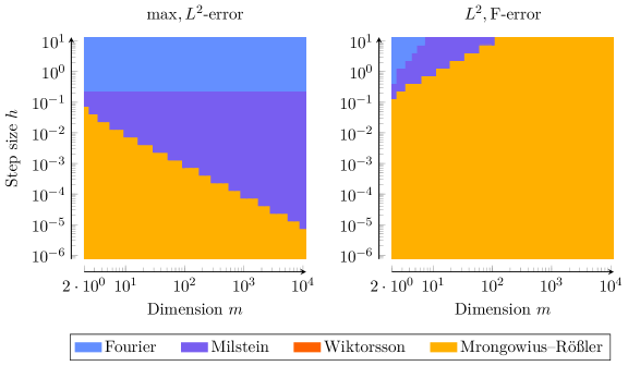
Abbildung 1: Optimal algorithm given the dimension $m$ and the step size $h$ in the respective norm for $\bar{\varepsilon}=h^{3/2}$.

The first thing we see is that the Wiktorsson algorithm is never the best choice in these scenarios. This is because for the Mrongowius--Rößler algorithm the required value of the truncation parameter can be reduced by a factor $\sqrt{5}$ while only requiring $m$ additional random numbers. Figure 1 confirms that this trade-off is always worth it, i.e., the Mrongowius--Rößler algorithm always outperforms the Wiktorsson algorithm.

Moreover, for the $\max,L^{2}$-error we see in the left plot of Figure 1 that if we fix some step size then there always exists some sufficiently high dimension such that it will be more efficient to apply the Milstein algorithm. This is a consequence of the higher order dependency on the dimension of the Mrongowius--Rößler algorithm (and also for the Wiktorsson algorithm) compared to the Milstein algorithm which dominates the error for large enough dimension if the step size is fixed. This means the Milstein algorithm is the optimal choice in this setting.

However, for any fixed dimension of the Wiener process (as it is the case for, e.g., SDEs) there always exists some threshold step size such that for all step sizes smaller than this threshold the Mrongowius--Rößler algorithm is more efficient than the other algorithms. This is due to the higher order of convergence in time of the Mrongowius--Rößler algorithm. Thus, as the step size tends to zero or if the step size is sufficiently small, the Mrongowius--Rößler algorithm is the optimal choice.

The situation in the right plot of Figure 1 for the $L^{2},\mathrm{F}$-error is different, because the simple scaling factor due to Lemma 1 does not translate into a simple scaling of the associated cost. Indeed it is no simple scaling at all if the cost contains additive terms independent of the error. Instead, only the error-dependent part of the cost is scaled by $m^{2}-m$ for the Fourier and Milstein algorithms and by $\sqrt{m^{2}-m}$ for the Wiktorsson and Mrongowius--Rößler algorithms (cf. Table 2). This is due to the different exponents of the truncation parameter in the corresponding error estimates. As a result of this, for the $L^{2},\mathrm{F}$-error the Mrongowius--Rößler algorithm is the optimal choice except for the particular case of a rather big step size and a low dimension of the Wiener process.

5.2 A study on the order of convergence

Convergence plots are an appropriate tool to complement theoretical convergence results with numerical simulations. Unfortunately, studying the convergence of random variables can be difficult, especially if the target (limit) random variable that has to be approximated can not be simulated exactly because its distribution is unknown. One way out of this problem is to substitute the target random variable by a highly accurate approximate random variable that allows to draw realizations from its known distribution.

In the present simulation study, we substitute the target random variable $\mathcal{I}(h)$ by the approximate random variable $\mathcal{I}^{\mathrm{ref},(p_{\mathrm{ref}})}(h)=\hat{\mathcal{I}}^{\mathrm{FS},(p_{\mathrm{ref}})}(h)$ based on the fundamental and accepted Fourier algorithm with high accuracy due to some large value for the parameter $p_{\mathrm{ref}}$. Therefore, we refer to $\mathcal{I}^{\mathrm{ref},(p_{\mathrm{ref}})}(h)$ as the reference random variable and let $\hat{\mathcal{I}}^{\mathrm{Alg},{(p)}}(h)$ denote the approximation based on one of the algorithms described in Section 3. We focus on the $\max,L^{2}$-error and the $L^{2},\mathrm{F}$-error of the approximation algorithms that we want to compare. We proceed as follows: Let $p_{\mathrm{ref}}\in\mathbb{N}$ be sufficiently large. First, some realizations of $W_{h}$ and the reference random variable $\mathcal{I}^{\mathrm{ref},(p_{\mathrm{ref}})}(h)$ are simulated. Then, the corresponding realizations of the Fourier coefficients $\alpha_{r}$ and $\beta_{r}$ for $1\leq r\leq p_{\mathrm{ref}}$ are stored together with $W_{h}$. Next, the approximations $\hat{\mathcal{I}}^{\mathrm{Alg},{(p)}}(h)$ are calculated based on the same realization, which has to be done carefully. The stored Fourier coefficients and the stored increment of the Wiener process are used to compute approximate solutions using each of the algorithms with a truncation parameter $p\ll p_{\mathrm{ref}}$. Especially, we are able to exactly extract from the stored Fourier coefficients and the stored increment of the Wiener process the corresponding realizations of the underlying standard Gaussian random variables that are used in Wiktorsson’s algorithm as well as in the Mrongowius--Rößler algorithm to approximate the tail.

To be precise, set $h=1$ and choose a large value $p_{\mathrm{ref}}$ for the reference random variable, for example $p_{\mathrm{ref}}=10^{6}$. Now, simulate and store the Wiener increment $W_{h}$ as well as the Fourier coefficients $\alpha_{r}^{i}$ and $\beta_{r}^{i}$ for $i=1,\ldots,m$ and $r=1,\ldots,p_{\mathrm{ref}}$. Then, calculate the reference random variable $\mathcal{I}^{\mathrm{ref},(p_{\mathrm{ref}})}(h)$ using the Fourier algorithm. Since every realization of the reference random variable $\mathcal{I}^{\mathrm{ref}}(h)$ is also an approximation to some realization of the random variable $\mathcal{I}(h)$, we can control the precision in $\max,L^{2}$-norm of the reference random variable exactly due to (63), i.e., it holds

$$\big{\|}\mathcal{I}(h)-\mathcal{I}^{\mathrm{ref},(p_{\mathrm{ref}})}(h)\big{\|}_{{\max,L^{2}}}=\bigg{(}\frac{3h^{2}}{2\pi^{2}}\bigg{(}\frac{\pi^{2}}{6}-\sum_{r=1}^{p_{\mathrm{ref}}}\frac{1}{r^{2}}\bigg{)}\bigg{)}^{\frac{1}{2}}\,.$$

For a large enough value of $p_{\mathrm{ref}}$ this error will be sufficiently small such that it can be neglected in our considerations. This justifies to work with the reference random variable.

Next, choose a truncation value $p\ll p_{\mathrm{ref}}$ for the approximation under consideration. First, calculate $\hat{\mathcal{I}}^{\mathrm{FS},(p)}(h)$ by the Fourier algorithm using only the first $p$ stored Fourier coefficients. Then, extract the necessary standard Gaussian vectors from the remaining stored Fourier coefficients using (25), (35), (37) and (50), i.e., calculate

$$\gamma_{1} =\frac{1}{\sqrt{\psi_{1}(p+1)}}\sum_{r=p+1}^{p_{\mathrm{ref}}}\frac{1}{r}\,\alpha_{r}\,,$$

$$\gamma =\frac{1}{\sqrt{2\psi_{1}(p+1)}}\Big{(}\Sigma^{(p)}\Big{)}^{-1/2}K_{m}(P_{m}-I_{m^{2}})\sum_{r=p+1}^{p_{\mathrm{ref}}}\frac{1}{r}\Big{(}\alpha_{r}\otimes\big{(}\beta_{r}-\sqrt{2}W_{h}\big{)}\Big{)}\,,$$

$$\gamma_{2} =\frac{1}{\sqrt{2\psi_{1}(p+1)}}\Big{(}\Sigma_{2}^{{(p)}}\Big{)}^{-1/2}K_{m}(P_{m}-I_{m^{2}})\sum_{r=p+1}^{p_{\mathrm{ref}}}\frac{1}{r}(\alpha_{r}\otimes\beta_{r})\,.$$

Calculating the vectors $\gamma_{1}$, $\gamma$ and $\gamma_{2}$ based on the already simulated and stored Fourier coefficients guarantees that they fit correctly together with the realization of the reference random variable. Note that for $r>p_{\mathrm{ref}}$ the Fourier coefficients $\alpha_{r}^{i}$ and $\beta_{r}^{i}$ for $i=1,\ldots,m$ of the reference random variable are all zero. Now, we calculate $\hat{\mathcal{I}}^{\mathrm{Mil},(p)}(h)$ by the Milstein, $\hat{\mathcal{I}}^{\mathrm{Wik},(p)}(h)$ by the Wiktorsson and $\hat{\mathcal{I}}^{\mathrm{MR},(p)}(h)$ by the Mrongowius--Rößler algorithm using only the first $p$ Fourier coefficients as well as $\gamma_{1}$, $\gamma$ and $\gamma_{2}$, respectively.

In Figure 2 the computed $\max,L^{2}$-errors are plotted versus the costs. Here, the cost is determined as the number of random numbers necessary to calculate the corresponding approximation for the iterated stochastic integral for each algorithm. To generate the random numbers we use the Mersenne Twister generator from Julia version 1.6. The steeper slope of the Wiktorsson and Mrongowius--Rößler algorithms can be clearly seen. This confirms the higher order of convergence of these algorithms in contrast to the Fourier and Milstein algorithms. Furthermore, it is interesting to observe that the Wiktorsson as well as the Mrongowius--Rößler algorithm perform better than their theoretical upper error bound given in Theorem 2. This gives reason to suspect that the error estimates for both algorithms given in Theorem 2 are not sharp.

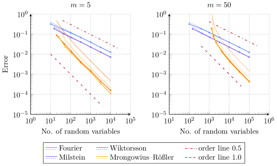
Abbildung 2: $\max,L^{2}$-error versus the number of random variables (cost) used for different dimensions of the Wiener process based on 100 realizations. The error is computed w.r.t. the reference random variable with $p_{\mathrm{ref}}=10^{6}$ and for $h=1$. The dotted lines show the corresponding theoretical error bounds according to Theorem 2.

6 A simulation toolbox for Julia and MATLAB

There exist several software packages to simulate SDEs in various programming languages. A short search brought up the following 20 toolboxes: for the C++ programming language [4, 25], for the Julia programming language [50, 48, 2, 49], for Mathematica [54], for Matlab [44, 22, 17, 52], for the Python programming language [3, 1, 15, 16, 36] and for the R programming language [23, 6, 18, 24]. However, only four of these toolboxes seem to contain an implementation of an approximation for the iterated stochastic integrals using Wiktorsson’s algorithm and none of them provide an implementation of the recently proposed Mrongowius--Rößler algorithm. To be precise, Wiktorsson’s algorithm is contained in the software packages SDELab [17] in Matlab as well as in its Julia continuation SDELab2.jl [50], in the Python package sdeint [1] and more recently also in the Julia package StochasticDiffEq.jl [49].

Note that among these four software packages only three have the source code readily available on GitHub:

• The software package SDELab2.jl does not seem to be maintained any more. It is worth mentioning that its implementation avoids the explicit use of Kronecker products. However, it is not as efficient as the implementations discussed in Section 3.3.3. Moreover, some simple test revealed that the implementation seems to suffer from some typos that may cause inexact results. Additionally, the current version of this package does not run with the current Julia version 1.6.

• The software package sdeint is purely written in Python and as such it is inherently slower than comparable implementations in a compiled language. Furthermore, it is based on a rather naïve implementation, e.g., explicitly constructing the Kronecker products and the permutation and selection matrices as described in Section 3.3.2. However, this is computational costly and thus rather inefficient, see also the discussion in Section 3.3.3.

• The software package StochasticDiffEq.jl offers the latest implementation of Wiktorsson’s approximation in the high-performance language Julia. Up to now, it is actively maintained and has a strong focus on good performance. It is basically a slightly optimized version of the SDELab2.jl implementation and thus it also does not achieve the maximal possible efficiency, especially compared to the discussion in Section 3.3.3.

In summary, there is currently no package providing an efficient algorithm for the simulation of iterated integrals. That is the main reason we provide a new simulation toolbox for Julia and Matlab that, among others, features Wiktorsson’s algorithm as well as the Mrongowius--Rößler algorithm. In Section 6.1 we present some more features of the toolbox. After giving usage examples in Section 6.2, we analyse the performance of our toolbox as compared to some existing implementations in Section 6.3.

6.1 Features of the new Julia and MATLAB simulation toolbox

We introduce a new simulation toolbox for the simulation of twofold iterated stochastic integrals and the corresponding Lévy areas for the Julia, see also [5], and Matlab programming languages. The aim of the toolbox is to provide both high performance and ease of use. On the one hand, experts can directly control each part of the algorithms. On the other hand, our software can automatically choose omitted parameters. Thus, a non-expert user only has to provide the Wiener increment and the associated step size and all other parameters will be chosen in an optimal way.

The toolbox is available as the software packages LevyArea.jl and LevyArea.m for Julia and Matlab, respectively. Both software packages are freely available from Netlib as the na57 package and from GitHub [27, 28]. Additionally, the Julia package is registered in the „General“ registry of Julia and can be installed using the built-in package manager, while the Matlab package is listed on the „Matlab Central - File Exchange“ and can be installed using the Add-On Explorer. This allows for an easy integration of these packages into other software projects.

Both packages provide the Fourier algorithm, the Milstein algorithm, the Wiktorsson algorithm and, to the best of our knowledge, for the first time the Mrongowius--Rößler algorithm. As the most important feature, all four algorithms are implemented following the insights from Section 3 to provide fast and highly efficient implementations. In Section 6.3 the performance of the Julia package is analysed in comparison to existing software.

Additional features include the ability to automatically choose the optimal algorithm based on the costs listed in Table 2. That is, given the increment of the driving Wiener process, the step size and an error bound in some norm, both software packages will automatically determine the optimal algorithm and the associated optimal value for the truncation parameter. Recall that optimal always means in terms of the number of random numbers that have to be generated in order to obtain minimal computing time. Thus, using the option for an optimal choice of the algorithm results in the best possible performance for each setting. Especially, for the simulation of SDE solutions with some strong order $1$ numerical scheme, both software packages can determine all necessary parameters by passing only the Wiener increment and the step size to the toolbox. Everything else is determined automatically such that the global order of convergence of the numerical integrator is preserved.

Furthermore, it is possible to directly simulate iterated stochastic integrals based on $Q$-Wiener processes on finite-dimensional spaces as they typically appear for the approximate simulation of solutions to SPDEs. In that case, the eigenvalues of the covariance operator $Q$ need to be passed to the software toolbox in order to compute the correctly scaled iterated stochastic integrals. This scaling is briefly described at the end of Section 2.1, see also [34] for a detailed discussion.

6.2 Usage of the software package

Next, we give some basic examples how to make use of the two software packages LevyArea.jl for Julia and LevyArea.m for Matlab. The aim is not to give a full documentation but rather to show some example invocations of the main functions. For more information we refer to the documentation that comes with the software and can be easily accessed in Julia and Matlab.

6.2.1 The Julia package LevyArea.jl

The following code works with Julia version 1.6. First of all, the software package LevyArea.jl [27] needs to be installed to make it available. Therefore, start Julia and enter the package manager by typing ] (a closing square bracket). Then execute

p

which downloads the package and adds it to the current project. After the installation of the package, one can load the package and initialize some variables that we use in the following:

⬇

j

julia> m = 5; # dimension of Wiener process

julia> h = 0.01; # step size or length of time interval

julia> err = 0.05; # error bound

julia> W = sqrt(h) * randn(m); # increment of Wiener process

Here, $W$ is the $m$-dimensional vector of increments of the driving Wiener process on some time interval of length $h$.

For the simulation of the corresponding twofold iterated stochastic integrals, one can use the following default call of the function iterated_integrals where only the increment and the step size are mandatory:

j

In this example, the error $\bar{\varepsilon}$ is not explicitly specified. Therefore, the function assumes the desired precision to be $\bar{\varepsilon}=h^{3/2}$ as it has to be chosen for the numerical solution of SDEs, see end of Section 4, and automatically chooses the optimal algorithm according to the logic in Section 5.1, see also Figure 1. If not stated otherwise, the default error criterion is the $\max,L^{2}$-error and the function returns the $m\times m$ matrix II containing a realization of the approximate iterated stochastic integrals that correspond to the given increment $W$.

The desired precision $\bar{\varepsilon}$ can be optionally provided using a third positional argument:

j

Again, the software package automatically chooses the optimal algorithm as analysed in Section 5.1.

To determine which algorithm is chosen by the package without simulating any iterated stochastic integrals yet, the function optimal_algorithm can be used. The arguments to this function are the dimension of the Wiener process, the step size and the desired precision:

j

It is also possible to choose the algorithm directly using the keyword argument alg. The value can be one of Fourier(), Milstein(), Wiktorsson() and MronRoe():

j

As the norm for the considered error, e.g., the $\max,L^{2}$- and $L^{2},\mathrm{F}$-norm can be selected using a keyword argument. The accepted values are MaxL2() and FrobeniusL2():

j

If iterated stochastic integrals for some $Q$-Wiener process need to be simulated, like for the numerical simulation of solutions to SPDEs, then the increment of the $Q$-Wiener process together with the square roots of the eigenvalues of the associated covariance operator have to be provided, see Section 2.1:

⬇

j

julia> QW = sqrt(h) * sqrt.(q) .* randn(m); # Q-Wiener increment

julia> IIQ = iterated_integrals(QW,sqrt.(q),h,err)

In this case, the function iterated_integrals utilizes a scaling of the iterated stochastic integrals as explained in Section 2.1 and also adjusts the error estimates appropriately such that the error bound holds w.r.t. the iterated stochastic integrals $\mathcal{I}^{Q}(h)$ based on the $Q$-Wiener process. Here the error norm defaults to the $L^{2},\mathrm{F}$-error.

Note that all discussed keyword arguments are optional and can be combined as favoured. Additional information can be found using the Julia help mode:

⬇

j

julia> ?optimal_algorithm

6.2.2 The MATLAB package LevyArea.m

The following code works with Matlab version 2020a. The installation of the software package LevyArea.m [28] in Matlab is done either by copying the package folder +levyarea into the current working directory or by installing the Matlab toolbox file LevyArea.mltbx. This can also be done through the Add-On Explorer.

The main function of the toolbox is the function iterated_integrals. It can be called by prepending the package name levyarea.iterated_integrals. However, since this may be cumbersome one can import the used functions once by

⬇

>

>> import levyarea.optimal_algorithm

and then one can omit the package name by simply calling iterated_integrals or optimal_algorithm, respectively. In the following, we assume that the two functions are imported, so that we can always call them directly without the package name.

For the examples considered next we initialize some auxiliary variables:

⬇

>

>> h = 0.01; % step size or length of time interval

>> err = 0.05; % error bound

>> W = sqrt(h) * randn(m,1); % increment of Wiener process

Note that $W$ denotes the $m$-dimensional vector of increments of the Wiener process on some time interval of length $h$.

For directly simulating the twofold iterated stochastic integrals given the increment of the Wiener process, one can call the main function iterated_integrals passing the increment and the step size:

>

These two parameters are mandatory. In this case, the precision is set to the default $\bar{\varepsilon}=h^{3/2}$ and the optimal algorithm is applied automatically according to Section 5.1 (see also Figure 1). The default norm for the error is set to be the $\max,L^{2}$-norm.

The desired precision $\bar{\varepsilon}$ can be optionally provided using a third positional argument:

>

Here, again the software package automatically chooses the optimal algorithm as analysed in Section 5.1.

In order to determine which algorithm is optimal for some given parameters without simulating the iterated stochastic integrals yet, the function optimal_algorithm can be used:

>

The arguments to this function are the dimension of the Wiener process, the step size and the desired precision.

On the other hand, it is also possible to choose the used algorithm directly using a key-value pair. The value can be one of 'Fourier', 'Milstein', 'Wiktorsson' and 'MronRoe'. E.g., to use the Milstein algorithm call:

>

The desired norm for the prescribed error bound can also be selected using a key-value pair. The accepted values are 'MaxL2' and 'FrobeniusL2' for the $\max,L^{2}$- and $L^{2},\mathrm{F}$-norm, respectively. E.g., in order to use the $L^{2},\mathrm{F}$-norm call:

>

The simulation of numerical solutions to SPDEs often requires iterated stochastic integrals based on $Q$-Wiener processes. In that case, the square roots of the eigenvalues of the associated covariance operator need to be provided. Therefore, first define all necessary variables and then call the function iterated_integrals using the key 'QWiener' as follows:

⬇

>

>> QW = sqrt(h) * sqrt(q) .* randn(m,1); % Q-Wiener increment

>> IIQ = iterated_integrals(QW,h,err,'QWiener',sqrt(q))

In this case, the function utilizes the scaling of the iterated stochastic integrals as explained in Section 2.1 and it also adjusts the error estimates w.r.t. $\mathcal{I}^{Q}(h)$ appropriately.

Note that all discussed keyword arguments (key-value pairs) are optional and can be combined as desired. Additional information can be found using the help function:

⬇

>

>> help levyarea.optimal_algorithm

6.3 Benchmark comparison

To assess the performance of the new software package, we compare it with some existing implementations. Therefore, we consider the software packages SDELab2.jl [50], sdeint [1] and StochasticDiffEq.jl [49]. First, the software package sdeint is completely written in Python and a quick simulation example with $m=50$, $h=0.01$, $\varepsilon=0.001$ and thus $p=15$ takes $9.9$ seconds to generate the matrix of iterated integrals with Wiktorsson’s algorithm. For the same parameters, our implementation of Wiktorsson’s algorithm in the package LevyArea.jl completed in only $5.5\cdot 10^{-6}$ seconds. This is a speed-up by a factor $1.8\times 10^{6}$ and therefore we exclude the Python package sdeint from our further comparison. Moreover, since the package SDELab2.jl seems to be unmaintained and does not run unmodified on current Julia versions, it is excluded from our benchmark as well. Thus, we compare the new package LevyArea.jl with the implementation in the package StochasticDiffEq.jl in the following.

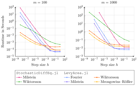
Abbildung 3: Runtime of the algorithms for variable step size and two different dimensions of the underlying Wiener process. The value of the truncation parameter is always chosen to guarantee that $\lVert\mathcal{I}-\hat{\mathcal{I}}\rVert_{\max,L^{2}}\leq h^{3/2}$ according to the error estimates in Theorem 2. The timings are averaged over 100 repetitions.

Algorithm A from	Algorithm B from	Relative speed-up ($\frac{t_{\text{{A}}}}{t_{\text{{B}}}}$)
StochasticDiffEq.jl	LevyArea.jl	$m=100$	$m=1000$
Milstein	Milstein	$1.5\times$--$14.8\times$	$1.5\times$--$196.8\times$
Wiktorsson	Wiktorsson	$2.1\times$--$25.1\times$	$3.0\times$--$165.8\times$
Wiktorsson	Mrongowius--Rößler	$6.2\times$--$52.1\times$	$4.4\times$--$356.1\times$

Tabelle 3: Minimal and maximal relative speed-ups of the new implementations in LevyArea.jl with respect to the implementations in StochasticDiffEq.jl for two different dimensions of the underlying Wiener process. See also Figure 3.

For the benchmark we measure the time it takes to generate the full matrix of iterated stochastic integrals over a range of step sizes and for two different dimensions of the driving Wiener process. To deal with measurement noise, we average the computing times over 100 runs. Further, in order to guarantee a fair comparison, we calculate the value of the truncation parameter according to Table 2 for all algorithms under consideration. We consider the setting where a strong order $1$ numerical scheme is applied for the simulation of solutions to SDEs. This setting is of high importance for many applications and a typical situation where iterated stochastic integrals need to be efficiently simulated. In order to retain the strong order $1$ if the twofold iterated stochastic integrals are replaced by their approximations, we need to choose the precision for the simulated iterated stochastic integrals following the discussion at the end of Section 4. Therefore, the error is always chosen as $\bar{\varepsilon}=h^{3/2}$ in the $\max,L^{2}$-norm and we consider step sizes $10^{0},10^{-1},\ldots,10^{-8}$ for the case $m=100$. For the case of $m=1000$, we initially use the same step sizes, however we refrain from applying the smaller step sizes for the Fourier and Milstein algorithms whenever the computing time or the needed memory becomes too large for reasonable computations.

The Julia package StochasticDiffEq.jl is used at version 6.37.1 and we run the in-place function StochasticDiffEq.get_iterated_I!(h,W,nothing,iip,p) where iip is a preallocated buffer. Note that the creation of this buffer is not included in our computing time measurements. The newly proposed Julia package LevyArea.jl is used at its current version 1.0.0. The benchmark is performed on a computer with an Intel Xeon E3-1245 v5 CPU at 3.50 GHz and 32 GB of memory using Julia version 1.6. Furthermore, the Julia package DrWatson.jl [9] is employed. The simulation results for both settings with $m=100$ and $m=1000$ are shown in Figure 3.

Considering the benchmark results in Figure 3, we can see that Wiktorsson’s algorithm as well as the Mrongowius--Rößler algorithm attain a higher order of convergence compared to the Fourier and the Milstein algorithms. This confirms the theoretical results in Theorem 2. Moreover, the simulation results show that for the Milstein algorithm as well as for Wiktorsson’s algorithm the implementation in the newly proposed package LevyArea.jl (blue, purple, orange and yellow colours) clearly outperforms the implementations in the package StochasticDiffEq.jl (red and green colours). This is due to the ideas for an efficient implementation presented in Section 3 that are incorporated in the package LevyArea.jl. This allows for a speed-up by factors up to 165.8 for Wiktorsson’s algorithm in the case of $m=1000$ for the range of parameters we tested.

Comparing the cases $m=100$ and $m=1000$, it seems that the implementations in the package StochasticDiffEq.jl have a much higher overhead for high-dimensional Wiener processes.

Moreover, it can be seen that for both settings the Mrongowius--Rößler algorithm is the best algorithm for sufficiently small step sizes as they typically arise for SDE and SPDE approximation problems. This confirms the theoretical results presented in Figure 1.

The relative speed-up of the implementations in package LevyArea.jl compared to package StochasticDiffEq.jl are specified in Table 3. There is a serious speed-up for each algorithm in the package LevyArea.jl that becomes even greater when step sizes are getting smaller or if the dimension of the Wiener process is rather high. Thus, the proposed software package LevyArea.jl allows for very efficient simulations of iterated stochastic integrals with very good performance also for small step sizes and small error bounds as well as for high dimensional Wiener processes. This makes the package valuable especially for SDE and SPDE simulations based on higher order approximation schemes.

- [1] Matthew Aburn ‘‘sdeint’’, 2021 URL: https://github.com/mattja/sdeint
- [2] Carl Åkerlindh ‘‘SDEModels.jl’’, 2019 URL: https://github.com/Godisemo/SDEModels.jl
- [3] Gerrit Ansmann ‘‘Efficiently and easily integrating differential equations with JiTCODE, JiTCDDE, and JiTCSDE’’ In Chaos 28.4 AIP Publishing, 2018 DOI: 10.1063/1.5019320
- [4] Eleftherios Avramidis, Marta Lalik and Ozgur E. Akman ‘‘SODECL: An Open-Source Library for Calculating Multiple Orbits of a System of Stochastic Differential Equations in Parallel’’ In ACM Trans. Math. Software 46.3 Association for Computing Machinery (ACM), 2020, pp. 1–21 DOI: 10.1145/3385076
- [5] Jeff Bezanson, Alan Edelman, Stefan Karpinski and Viral B. Shah ‘‘Julia: A fresh approach to numerical computing’’ In SIAM Rev. 59.1 SIAM, 2017, pp. 65–98 DOI: 10.1137/141000671
- [6] Alexandre Brouste et al. ‘‘The YUIMA Project: A Computational Framework for Simulation and Inference of Stochastic Differential Equations’’ In J. Stat. Softw. 57.4 Foundation for Open Access Statistic, 2014 DOI: 10.18637/jss.v057.i04
- [7] J... Clark and R.. Cameron ‘‘The maximum rate of convergence of discrete approximations for stochastic differential equations’’ In Stochastic Differential Systems Filtering and Control. Lecture Notes in Control and Information Sciences Springer, 1980, pp. 162–171 DOI: 10.1007/BFb0004007
- [8] G. Da Prato and J. Zabczyk ‘‘Stochastic equations in infinite dimensions’’ 152, Encyclopedia of Mathematics and its Applications Cambridge University Press, Cambridge, 2014, pp. xviii+493 DOI: 10.1017/CBO9781107295513
- [9] George Datseris, Jonas Isensee, Sebastian Pech and Tamás Gál ‘‘DrWatson: the perfect sidekick for your scientific inquiries’’ In J. Open Source Softw. 5.54 The Open Journal, 2020 DOI: 10.21105/joss.02673
- [10] Alexander Davie ‘‘KMT theory applied to approximations of SDE’’ In Stochastic analysis and applications 2014 Springer Cham, 2014, pp. 185–201 DOI: 10.1007/978-3-319-11292-3_7
- [11] Andrew S. Dickinson ‘‘Optimal approximation of the second iterated integral of Brownian motion’’ In Stoch. Anal. Appl. 25.5, 2007, pp. 1109–1128 DOI: 10.1080/07362990701540592
- [12] Guy Flint and Terry Lyons ‘‘Pathwise approximation of SDEs by coupling piecewise abelian rough paths’’ In arXiv e-prints, 2015 arXiv:1505.01298 [math.PR]
- [13] James Foster and Karen Habermann ‘‘Brownian bridge expansions for Lévy area approximations and particular values of the Riemann zeta function’’ In Combin. Probab. Comput. Cambridge University Press, 2022 DOI: 10.1017/s096354832200030x
- [14] J.. Gaines and T.. Lyons ‘‘Random generation of stochastic area integrals’’ In SIAM J. Appl. Math. 54.4 SIAM, 1994, pp. 1132–1146 DOI: 10.1137/S0036139992235706
- [15] M.. Gevorkyan et al. ‘‘Stochastic Runge–Kutta Software Package for Stochastic Differential Equations’’ In Dependability Engineering and Complex Systems Springer International Publishing, 2016, pp. 169–179 DOI: 10.1007/978-3-319-39639-2_15
- [16] Migran N. Gevorkyan, Anastasiya V. Demidova, Anna V. Korolkova and Dmitry S. Kulyabov ‘‘Issues in the Software Implementation of Stochastic Numerical Runge–Kutta’’ In Developments in Language Theory Springer International Publishing, 2018, pp. 532–546 DOI: 10.1007/978-3-319-99447-5_46
- [17] Hagen Gilsing and Tony Shardlow ‘‘SDELab: A package for solving stochastic differential equations in MATLAB’’ In J. Comput. Appl. Math. 205.2 Elsevier BV, 2007, pp. 1002–1018 DOI: 10.1016/j.cam.2006.05.037
- [18] Arsalane Chouaib Guidoum and Kamal Boukhetala ‘‘Performing Parallel Monte Carlo and Moment Equations Methods for Itô and Stratonovich Stochastic Differential Systems: R Package Sim.DiffProc’’ In J. Stat. Softw. 96.2 Foundation for Open Access Statistic, 2020 DOI: 10.18637/jss.v096.i02
- [19] Claudine Hallern and Andreas Rößler ‘‘A derivative-free Milstein type approximation method for SPDEs covering the non-commutative noise case’’ In Stoch. Partial Differ. Equ. Anal. Comput. Springer ScienceBusiness Media LLC, 2022 DOI: 10.1007/s40072-022-00274-6
- [20] Claudine Hallern and Andreas Rößler ‘‘An analysis of the Milstein scheme for SPDEs without a commutative noise condition’’ In Monte Carlo and quasi-Monte Carlo methods. MCQMC 2018. Proceedings of the 13th international conference on Monte Carlo and quasi-Monte Carlo methods in scientific computing, Rennes, France, July 1--6, 2018 Springer Cham, 2020, pp. 503–521 DOI: 10.1007/978-3-030-43465-6_25
- [21] Harold V. Henderson and S.. Searle ‘‘The vec-permutation matrix, the vec operator and Kronecker products: a review’’ In Linear Multilinear Algebra 9.4 Informa UK Limited, 1981, pp. 271–288 DOI: 10.1080/03081088108817379
- [22] Andrew D. Horchler ‘‘SDETools’’, 2013 URL: https://github.com/horchler/SDETools
- [23] Stefano M. Iacus ‘‘Simulation and Inference for Stochastic Differential Equations’’ Springer New York, 2008 DOI: 10.1007/978-0-387-75839-8
- [24] Stefano M. Iacus and Nakahiro Yoshida ‘‘Simulation and Inference for Stochastic Processes with YUIMA’’ Springer International Publishing, 2018 DOI: 10.1007/978-3-319-55569-0
- [25] Aleksander Janicki, Adam Izydorczyk and Przemyslaw Gradalski ‘‘Computer simulation of stochastic models with SDE-Solver software package’’ In Computational science -- ICCS 2003. International conference, Melbourne, Australia and St. Petersburg, Russia, June 2--4, 2003. Proceedings, Part I Springer Berlin, 2003, pp. 361–370 DOI: 10.1007/3-540-44860-8_37
- [26] Ioannis Karatzas and Steven E. Shreve ‘‘Brownian Motion and Stochastic Calculus’’ Springer-Verlag, 1991 DOI: 10.1007/978-1-4612-0949-2
- [27] Felix Kastner and Andreas Rößler ‘‘LevyArea.jl’’ Zenodo, 2022 DOI: 10.5281/zenodo.5883748
- [28] Felix Kastner and Andreas Rößler ‘‘LevyArea.m’’ Zenodo, 2022 DOI: 10.5281/zenodo.5883929
- [29] P.. Kloeden and E. Platen ‘‘Numerical solution of stochastic differential equations’’ 23, Applications of Mathematics Springer Berlin, 1995, pp. xxxvi+632 DOI: 10.1007/978-3-662-12616-5
- [30] P.. Kloeden, E. Platen and I.. Wright ‘‘The approximation of multiple stochastic integrals’’ In Stoch. Anal. Appl. 10.4, 1992, pp. 431–441 DOI: 10.1080/07362999208809281
- [31] D.. Kuznetsov ‘‘A Comparative Analysis of Efficiency of Using the Legendre Polynomials and Trigonometric Functions for the Numerical Solution of Ito Stochastic Differential Equations’’ In Comput. Math. Math. Phys. 59.8 Pleiades Publishing Ltd, 2019, pp. 1236–1250 DOI: 10.1134/s0965542519080116
- [32] D.. Kuznetsov ‘‘Development and Application of the Fourier Method for the Numerical Solution of Ito Stochastic Differential Equations’’ In Comput. Math. Math. Phys. 58.7 Pleiades Publishing Ltd, 2018, pp. 1058–1070 DOI: 10.1134/s0965542518070096
- [33] Claudine Leonhard and Andreas Rößler ‘‘Enhancing the order of the Milstein scheme for stochastic partial differential equations with commutative noise’’ In SIAM J. Numer. Anal. 56.4, 2018, pp. 2585–2622 DOI: 10.1137/16M1094087
- [34] Claudine Leonhard and Andreas Rößler ‘‘Iterated stochastic integrals in infinite dimensions: approximation and error estimates’’ In Stoch. Partial Differ. Equ. Anal. Comput. 7.2, 2019, pp. 209–239 DOI: 10.1007/s40072-018-0126-9
- [35] Paul Lévy ‘‘Wiener’s random function, and other Laplacian random functions’’ In Proceedings of the Second Berkeley Symposium on Mathematical Statistics and Probability, 1950 University of California Press, BerkeleyLos Angeles, 1951, pp. 171–187
- [36] Xuechen Li ‘‘torchsde’’, 2021 URL: https://github.com/google-research/torchsde
- [37] Horst Liske, Eckhard Platen and Wolfgang Wagner ‘‘About mixed multiple Wiener integrals’’ In Preprint P-Math-23/82, IMath, Akad. der Wiss. der DDR, Prepr., Akad. Wiss. DDR, Inst. Math. P-MATH-23/82, 17 p. (1982)., 1982
- [38] Jan R. Magnus and H. Neudecker ‘‘The commutation matrix: some properties and applications.’’ In Ann. Statist. 7.2 The Institute of Mathematical Statistics, 1979, pp. 381–394 DOI: 10.1214/aos/1176344621
- [39] Simon J.. Malham and Anke Wiese ‘‘Efficient almost-exact Lévy area sampling’’ In Statist. Probab. Lett. 88 Elsevier (North-Holland), Amsterdam, 2014, pp. 50–55 DOI: 10.1016/j.spl.2014.01.022
- [40] G.. Milstein ‘‘Numerical integration of stochastic differential equations’’ Translated and revised from the 1988 Russian original 313, Mathematics and its Applications Kluwer Academic Publishers, Dordrecht, 1995, pp. viii+169 DOI: 10.1007/978-94-015-8455-5
- [41] Jan Mrongowius and Andreas Rößler ‘‘On the approximation and simulation of iterated stochastic integrals and the corresponding Lévy areas in terms of a multidimensional Brownian motion’’ In Stoch. Anal. Appl. 40.3 Taylor & Francis, 2022, pp. 397–425 DOI: 10.1080/07362994.2021.1922291
- [42] A. Neuenkirch, S. Tindel and J. Unterberger ‘‘Discretizing the fractional Lévy area’’ In Stochastic Process. Appl. 120.2 Elsevier (North-Holland), Amsterdam, 2010, pp. 223–254 DOI: 10.1016/j.spa.2009.10.007
- [43] Andreas Neuenkirch and Taras Shalaiko ‘‘The maximum rate of convergence for the approximation of the fractional Lévy area at a single point’’ In J. Complexity 33 Elsevier (Academic Press), San Diego, CA, 2016, pp. 107–117 DOI: 10.1016/j.jco.2015.09.008
- [44] Umberto Picchini ‘‘SDE Toolbox’’, 2017 URL: http://sdetoolbox.sourceforge.net
- [45] C. Prévôt and M. Röckner ‘‘A concise course on stochastic partial differential equations’’ 1905, Lecture Notes in Mathematics Springer Berlin, 2007, pp. vi+144 DOI: 10.1007/978-3-540-70781-3
- [46] A. Rößler ‘‘Runge-Kutta methods for the strong approximation of solutions of stochastic differential equations’’ In SIAM J. Numer. Anal. 48.3, 2010, pp. 922–952 DOI: 10.1137/09076636X
- [47] Tobias Rydén and Magnus Wiktorsson ‘‘On the simulation of iterated Itô integrals’’ In Stochastic Process. Appl. 91.1, 2001, pp. 151–168 DOI: 10.1016/S0304-4149(00)00053-3
- [48] Moritz Schauer ‘‘Bridge.jl’’, 2021 URL: https://github.com/mschauer/Bridge.jl
- [49] SciML ‘‘StochasticDiffEq.jl’’, 2021 URL: https://github.com/SciML/StochasticDiffEq.jl
- [50] Tony Shardlow ‘‘SDELab2’’, 2016 URL: https://github.com/tonyshardlow/SDELAB2
- [51] David M. Stump and James M. Hill ‘‘On an infinite integral arising in the numerical integration of stochastic differential equations’’ In Proc. R. Soc. A 461.2054 Royal Society Publishing, London, 2005, pp. 397–413 DOI: 10.1098/rspa.2004.1379
- [52] The MathWorks, Inc. ‘‘Financial Toolbox’’, 2021 URL: https://www.mathworks.com/help/finance/
- [53] M. Wiktorsson ‘‘Joint characteristic function and simultaneous simulation of iterated Itô integrals for multiple independent Brownian motions’’ In Ann. Appl. Probab. 11.2, 2001, pp. 470–487 DOI: 10.1214/aoap/1015345301
- [54] Wolfram Research ‘‘ItoProcess’’, 2016 URL: https://reference.wolfram.com/language/ref/ItoProcess.html