Unicorn: Reasoning about Configurable System Performance through the Lens of Causality

Abstract.

Modern computer systems are highly configurable, with the total variability space sometimes larger than the number of atoms in the universe. Understanding and reasoning about the performance behavior of highly configurable systems, over a vast and variable space, is challenging. State-of-the-art methods for performance modeling and analyses rely on predictive machine learning models, therefore, they become (i) unreliable in unseen environments (e.g., different hardware, workloads), and (ii) may produce incorrect explanations. To tackle this, we propose a new method, called Unicorn, which (i) captures intricate interactions between configuration options across the software-hardware stack and (ii) describes how such interactions can impact performance variations via causal inference. We evaluated Unicorn on six highly configurable systems, including three on-device machine learning systems, a video encoder, a database management system, and a data analytics pipeline. The experimental results indicate that Unicorn outperforms state-of-the-art performance debugging and optimization methods in finding effective repairs for performance faults and finding configurations with near-optimal performance. Further, unlike the existing methods, the learned causal performance models reliably predict performance for new environments.

1. Introduction

(a)

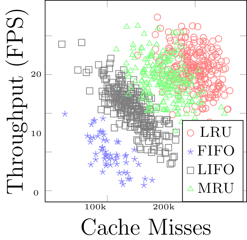
(b)

(c)

Figure 1. An example showing the effectiveness of causality in reasoning about system performance behavior. (a) Observational data shows that the increase in Cache Misses leads to high Throughput and such trend is typically captured by statistical reasoning in ML models; (b) incorporating Cache Policy as a confounder correctly shows increase of Cache Misses corresponding to decrease in Throughput; (c) the corresponding causal model correctly captures Cache Policy as a common cause to explain performance behavior.

Modern computer systems, such as data analytics pipelines, are typically composed of multiple components, where each component has a plethora of configuration options that can be deployed individually or in conjunction with other components on different hardware platforms. The configuration space of such highly configurable systems is combinatorially large, with 100s if not 1000s of software and hardware configuration options that interact non-trivially with one another (wang2018understanding; halin2019test; JC:MASCOTS16; velez2022study). Individual component developers typically have a relatively localized, and thus limited, understanding of the performance behavior of the systems that comprise the components. Therefore, developers and end-users of the final system are often overwhelmed with the complexity of composing and configuring components, making it challenging and error-prone to configure these systems to reach desired performance goals.

Incorrect configuration (misconfiguration) elicits unexpected interactions between software and hardware, resulting in non-functional faults, i.e., degradations in non-functional system properties like latency and energy consumption. These non-functional faults, unlike regular software bugs, do not cause the system to crash or exhibit any obvious misbehavior (reddy2016fault; tsakiltsidis2016automatic; nistor2013discovering). Instead, misconfigured systems remain operational but degrade in performance (bryant2003computer; molyneaux2009art; sanchez2020tandem; nistor2015caramel) that can cause major issues in cloud infrastructure (amazon:config:outage), internet-scale systems (fb:config:outage), and on-device machine learning (ML) systems (slowimag79:online). For example, a developer complained that “I have a complicated system composed of multiple components running on NVIDIA Nano and using several sensors and I observed several performance issues. (super_frustrated_power_perf:online).” In another instance, a developer asks “I’m quite upset with CPU usage on Jetson TX2 while running TCP/IP upload test program” (HighCPUu7:online). After struggling in fixing the issues over several days, the developer concludes, “there is a lot of knowledge required to optimize the network stack and measure CPU load correctly. I tried to play with every configuration option explained in the kernel documents.” In addition, they would like to understand the impact of configuration options and their interactions, e.g., “What is the effect of swap memory on increasing throughput? (slowimag79:online)”.

Existing works and gap. Understanding the performance behavior of configurable systems can enable (i) performance debugging (SGAK:ESECFSE15; GSKA:SPPEXA), (ii) performance tuning (H:CACM; SHM:LIO; H:AS; VPGFC:ICPE17; HPHL:ICSE15; WWHJK:GECCO15; NMSA:Arxive17; MARC:SPLC13; ORGC:SPLC14), and (iii) architecture adaptation (JGAP:CSMR13; ABDD:VISSOFT13; KK:WSR16; JVKSK:SEAMS17; HSCMAR:SIGPLAN; FHM:FSE15; EEM:TSE; EEM:FSE10). A common strategy is to build performance influence models such as regression models that explain the influence of individual options and their interactions (SGAK:ESECFSE15; VPGFC:ICPE17; GCASW:ASE13; pereira2019learning). These approaches are adept at inferring the correlations between configuration options and performance objectives, however, as illustrated in Fig. 1 performance influence models suffer from several shortcomings (detailed in §2): (i) they become  unreliable in unseen environments and (ii)  produce incorrect explanations.

Our approach.  Based on the several experimental pieces of evidence presented in the following sections, this paper proposes Unicorn–a methodology that enables reasoning about configurable system performance with causal inference and counterfactual reasoning. Unicorn first recovers the underlying causal structure from performance data. The causal performance model allows users to (i) identify the root causes of performance faults, (ii) estimate the causal effects of various configurable parameters on the performance objectives, and (iii) prescribe candidate configurations to fix the performance fault or optimize system performance.

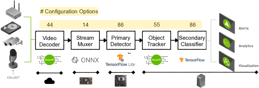
Figure 2. Deepstream: An example of a highly-configurable composed system, a big data analytics pipeline system, with several configurable components: (i) Video Decoder performs video encoding/decoding with different formats; (ii) Stream Muxer accepts input streams and converts them to sequential batch frames; (iii) Primary Detector transforms the input frames based on input NN requirements and makes model inference to detect objects; (iv) Object Tracker supports multi-object tracking; (v) Secondary Classifier improves performance by avoiding re-inferencing.

Contributions. Our contributions are as follows:

• We propose Unicorn (§4), a novel approach that allows causal reasoning about system performance.

• We have conducted a thorough evaluation of Unicorn in a controlled case study (§LABEL:sec:casestudy) as well as real-world large-scale experiments. In particular, we evaluated effectiveness (§LABEL:sec:effectiveness), transferability (§LABEL:sec:transfer), and scalability (§LABEL:sec:scalability) by comparing Unicorn with: (i) state-of-the-art performance debugging approaches, including CBI (song2014statistical), DD (artho2011iterative), EnCore (zhang2014encore), and BugDoc (lourencco2020bugdoc) and (ii) performance optimization techniques, including SMAC (hutter2011sequential) and PESMO (hernandez2016predictive). The evaluations were conducted on six real-world highly configurable systems, including a video analytic pipeline, Deepstream (DeepStream), three deep learning-based systems, Xception (chollet2017xception), Deepspeech (hannun2014deep), and BERT (devlin2018bert), a video encoder, X264 (x264), and a database engine, SQLite (SQLite), deployed on NVIDIA Jetson hardware (TX1, TX2, and Xavier).

• In addition to sample efficiency and accuracy of Unicorn in finding root causes of performance issues, we show that the learned causal performance model is transferable across different workload and deployment environments. Finally, we demonstrate the scalability of Unicorn to large systems consisting of 500 options and several trillion potential configurations.

• The artifacts and supplementary materials can be found at https://github.com/softsys4ai/unicorn.

2. Motivating Scenarios

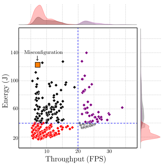
(a) Performance Distribution

(b) Misconfiguration

(b) (a) Performance distribution when Deepstream is deployed on NVIDIA Jetson Xavier (b) Misconfiguration that caused the multi-objective non-functional fault, shown as $\square$ in the performance distribution.

Simple motivating scenario. In this simple scenario, we motivate our work by demonstrating why performance analyses solely based on correlational statistics may lead to an incorrect outcome. Here, the collected performance data indicates that Throughput is positively correlated with increased Cache Misses (as in Fig. 1 (a)). A simple ML model built on this data will predict with high confidence that larger Cache Misses leads to higher Throughput—this is misleading as higher Cache Misses should, in theory, lower Throughput. By further investigating the performance data, we noticed that the caching policy was automatically changed during measurement. We then segregated the same data on Cache Policy (as in  Fig. 1 (b)) and found out that within each group of Cache Misses, as Cache Misses increases, the Throughput decreases. One would expect such behavior, as the more Cache Misses the higher number of access to external memory, and, therefore, the Throughput would be expected to decrease. The system resource manager may change the Cache Policy based on some criteria; this means that for the same number of Cache Misses, the Throughput may be lower or higher; however, in all Cache Policies, the increases of Cache Misses resulting in a decrease in Throughput. Thus, Cache Policy acts as a confounder that explains the relation between Cache Misses and Throughout, which a correlation-based model will not be able to capture. In contrast, a causal performance model, as shown in Fig. 1 (c), finds the relation between Cache Misses, Cache Policy, and Throughput and thus can reason about the observed behavior correctly.

In reality, performance analysis and debugging of heterogeneous multi-component systems is non-trivial and often compared with finding the needle in the haystack (whitaker2004configuration). In particular, the end-to-end performance analysis is not possible by reasoning about individual components in isolation, as components may interact with one another in such a composed system. Below, we use a highly configurable multi-stack system to motivate why causal reasoning is a better choice for understanding the performance behavior of complex systems.

Motivating scenario based on a highly configurable data analytics system. We deployed a data analytics pipeline, Deepstream (DeepStream). Deepstream has many components, and each component has many configuration options, resulting in several variants of the same system as shown in Fig. 2. Specifically, the variability arises from: (i) the configuration options of each software component in the pipeline, (ii) configurable low-level libraries that implement functionalities required by different components (e.g., the choice of tracking algorithm in the tracker or different neural network architectures), (iii) the configuration options associated with each component’s deployment stack (e.g., CPU Frequency of Xavier). Further, there exist many configurable events that can be measured/observed at the OS level by the event tracing system. More specifically, the configuration space of the system includes (i) 27 Software options (Decoder: 6, Stream Muxer: 7, Detector: 10, Tracker: 4), (ii) 22 Kernel options (e.g., Swappiness, Scheduler Policy, etc.), and (iii) 4 Hardware options (CPU Frequency, CPU Cores, etc.). We use 8 camera streams as the workload, x264 as the decoder, TrafficCamNet model that uses ResNet 18 architecture for the detector, and an NvDCF tracker, which uses a correlation filter-based online discriminative learning algorithm for tracking. Such a large space of variability makes performance analysis challenging. This is further exacerbated by the fact that the configuration options among the components interact with each other. Additional details about our Deepstream implementation can be found in the supplementary materials.

To better understand the potential of the proposed approach, we measured (i) application performance metrics including throughput and energy consumption by instrumenting the Deepstream code, and (ii) 288 system-wide performance events (hardware, software, cache, and tracepoint) using $perf$ and measured performance for 2461 configurations of Deepstream in two different hardware environments, Xavier, and TX2. As it is depicted in Fig. 3a, performance behavior of Deepstream, like other highly configurable systems, is non-linear, multi-modal, and non-convex (jamshidi2016uncertainty). In this work, we focus on two performance tasks: (i) Performance Debugging: here, one observes a performance issue (e.g., latency), and the task involves replacing the current configurations in the deployed environment with another that fixes the observed performance issue; (ii) Performance Optimization: here, no performance issue is observed; however, one wants to get a near-optimal performance by finding a configuration that enables the best trade-off in the multi-objective space (e.g., throughput vs. energy consumption vs. accuracy in Deepstream).

To show major shortcomings of existing state-of-the-art performance models, we built performance influence models that have extensively been used in the systems’ literature (siegmund2015performance; JSVKPA:ASE17; GCASW:ASE13; GSKA:SPPEXA; kolesnikov2019tradeoffs; kaltenecker2020interplay; muhlbauer2019accurate; grebhahn2019predicting; siegmund2020dimensions) and it is the standard approach in industry (kolesnikov2019tradeoffs; kaltenecker2020interplay). Specifically, we built non-linear regression models with forward and backward elimination using a step-wise training method on the Deepstream performance data. We then performed several sensitivity analyses and identified the following issues:

1. Performance influence models could not reliably predict performance in unseen environments. Performance behavior of configurable systems vary across environments, e.g., when we deploy software on new hardware with a different microarchitecture or when the workload changes (JSVKPA:ASE17; JVKSK:SEAMS17; JVKS:FSE18; iqbal_transfer_2019; VPGFC:ICPE17). When building a performance model, it is important to capture predictors that transfer well, i.e., remain stable across environmental changes. The predictors in performance models are options ($o_{i}$) and interactions ($\phi(o_{i}..o_{j})$) that appear in the explainable models of form $f(c)=\beta_{0}+\Sigma_{i}{\phi(o_{i})}+\Sigma_{i..j}{\phi(o_{i}..o_{j})}$. The transferability of performance predictors is expected from performance models since they are learned based on one environment (e.g., staging as the source environment) and are desirable to reliably predict performance in another environment (e.g., production as the target environment). Therefore, if the predictors in a performance model become unstable, even if they produce accurate predictions in the current environment, there is no guarantee that it performs well in other environments, i.e., they become unreliable for performance predictions and performance optimizations due to large prediction errors. To investigate how transferable performance influence models are across environments, we performed a thorough analysis when learning a performance model for DeepStream deployed on two different hardware platforms that have two different microarchitectures. Note that such environmental changes are common, and it is known that performance behavior changes when, in addition to a change in hardware resources (e.g., higher CPU Frequency), we have major differences in terms of architectural constructs (ding2021generalizable; curtsinger2013stabilizer), also supported by a thorough empirical study (JSVKPA:ASE17). The results in Fig. 4 (a) indicate that the number of stable predictors is too small for the total number of predictors that appear in the learned regression models. Additionally, the coefficients of the common predictors change across environments as shown in Fig. 5 making them unreliable to be resued in the new scenario.

2. Performance influence models could produce incorrect explanations. In addition to performance predictions, where developers are interested to know the effect of configuration changes on performance objectives, they are also interested to estimate and explain the effect of a change in particular configuration options (e.g., changing Cache Policy) toward performance variations. It is therefore desirable that the strength of the predictors in performance models, determined by their coefficients, remain consistent across environments (ding2021generalizable; JSVKPA:ASE17). In the context of our simple scenario in Fig. 1, the learned performance influence model indicates that $0.16\times\texttt{Cache Misses}$ is the most influential term that determines throughput, however, the (causal) model in Fig. 1 (c) show that the interactions between configuration option Cache Policy and system event Cache Misses is a more reliable predictor of the throughput, indicating that the performance influence model, due to relying on superficial correlational statistics, incorrectly explains factors that influence performance behavior of the system. The low Spearman rank correlation between predictors coefficients indicates that a performance model based on regression could be highly unstable and thus would produce unreliable explanations as well as unreliable estimation of the effect of change in specific options for performance debugging or optimization.

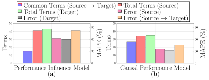
Figure 4. (a) Performance influence models do not generalize well as the number of common terms, total terms and prediction error of these models change from source (Xavier) to target (TX2). The rank correlation between source and target is 0.07 (p-value=0.73). (b) Causal performance models generalize better as the number of common terms, total terms and prediction error of the structural does not change much from source (Xavier) to target (TX2). The rank correlation between source and target is 0.49 (p-value=0.76).

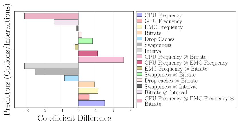
Figure 5. Visualizing co-efficient differences from the source (Xavier) performance influence model to the target (TX2) performance influence model for the common terms for both options and interactions (shown by $\otimes$).

3. Causal Reasoning for Systems

We hypothesize that the reason behind unreliable predictions and incorrect explanations of performance influence models (see §3) is the inability of correlation-based models to capture causally relevant predictors in the learned performance models. The theoretical and empirical results (JSVKPA:ASE17; javidian2019transfer) also show that predictive models that contain non-causal predictors, even though they might be accurate in the environment that the training data come from, such models are not typically transferable in unseen environments.

Hence, we introduce a new abstraction for performance modeling, called Causal Performance Model, which gives us the leverage for performing causal reasoning for computer systems. In particular, we introduce the causal performance model to serve as a modeling abstraction that allow building reusable performance models for downstream performance tasks, including performance predictions, performance testing and debugging, performance optimization, and more importantly, it serves as a transferable model that allow performance analyses across environments (JSVKPA:ASE17; javidian2019transfer).

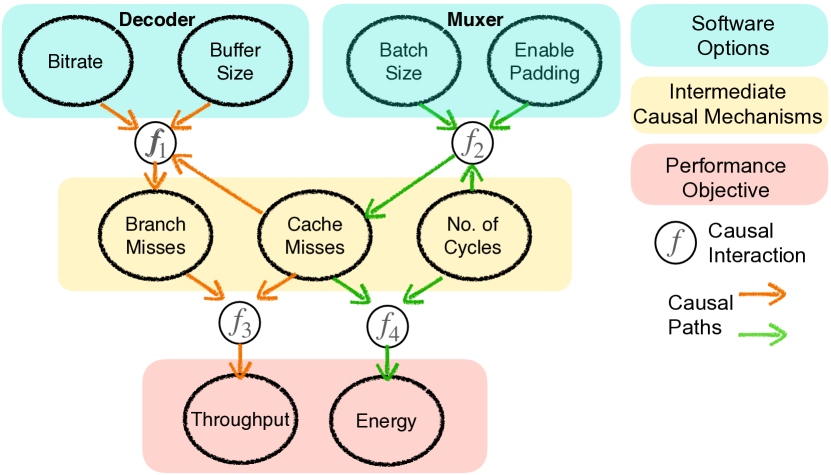
Figure 6. A partial causal performance model for Deepstream discovered in our experiments.

Causal performance models. We define a causal performance model as an instantiation of Probabilistic Graphical Models (pearl1998graphical) with new types and structural constraints to enable performance modeling and analyses. Formally, causal performance models (cf., Fig. 6) are Directed Acyclic Graphs (DAGs) (pearl1998graphical) with (i) performance variables, (ii) functional nodes that define functional dependencies between performance variables (i.e., how variations in one or multiple variables determine variations in other variables), (iii) causal links that interconnect performance nodes with each other via functional nodes, and (iv) constraints to define assumptions we require in performance modeling (e.g., software configuration options cannot be the child node of performance objectives; or Cache Misses as a performance variable takes only positive integer values). In particular, we define three new variable types: (i) Software-level configuration options associated with a software component in the composed system (e.g., Bitrate in the decoder component of Deepstream), and hardware-level options (e.g., CPU Frequency), (ii) intermediate performance variables relating the effect of configuration options to performance objectives including middleware traces (e.g., Context Switches), performance events (e.g., Cache Misses) and (iii) end-to-end performance objectives (e.g., Throughput). In this paper, we characterize the functional nodes with polynomial models, because of their simplicity and their explainable nature, however, they could be characterized with any functional forms, e.g., neural networks (xia2021causal; scherrer2021learning). We also define two specific constraints over causal performance models to characterize the assumptions in performance modeling: (i) defining variables that can be intervened (note that some performance variables can only be observed (e.g., Cache Misses) or in some cases where a variable can be intervened, the user may want to restrict the variability space, e.g., the cases where the user may want to use prior experience, restricting the variables that do not have a major impact to performance objectives); (ii) structural constraints, e.g., configuration options do not cause other options. Note that such constraints enable incorporating domain knowledge and enable further sparsity that facilitates learning with low sample sizes.

How causal reasoning can fix the reliability and explainability issues in current performance analyses practices?. The causal performance models contain more detail than the joint distribution of all variables in the model. For example, the causal performance model in Fig. 6 encodes not only Branch Misses and Throughput readings are dependent but also that lowering Cache Misses causes the Throughput of Deepstream to increase and not the other way around. The arrows in causal performance models correspond to the assumed direction of causation, and the absence of an arrow represents the absence of direct causal influence between variables, including configuration options, system events, and performance objectives. The only way we can make predictions about how performance distribution changes for a system when deployed in another environment or when its workload changes are if we know how the variables are causally related. This information about causal relationships is not captured in non-causal models, such as regression-based models. Using the encoded information in causal performance models, we can benefit from analyses that are only possible when we explicitly employ causal models, in particular, interventional and counterfactual analyses (pearl2009causality; pearl2018book). For example, imagine that in a hardware platform, we deploy the Deepstream and observed that the system throughput is below 30 FPS and Buffer Size as one of the configuration options was determined dynamically between 8k-20k. The system maintainers may be interested in estimating the likelihood of fixing the performance issue in a counterfactual world where the Buffer Size is set to a fixed value, 6k. The estimation of this counterfactual query is only possible if we have access to the underlying causal model because setting a specific option to a fixed value is an intervention as opposed to conditional observations that have been done in the traditional performance model for performance predictions.

Causal performance models are not only capable of predicting system performance in certain environments, they encode the causal structure of the underlying system performance behavior, i.e., the data-generating mechanism behind system performance. Therefore, the causal model can reliably transfer across environments (scholkopf2021toward). To demonstrate this for causal performance models as a particular characterization of causal models, we performed a similar sensitivity analysis to regression-based models and observed that causal performance models can reliably predict performance in unseen environments (see Fig. 4 (b)). In addition, as opposed to performance influence models that are only capable of performance predictions, causal performance models can be used for several downstream heterogeneous performance tasks. For example, using a causal performance model, we can determine the causal effects of configuration options on performance objectives. Using the estimated causal effects, one can determine the effect of change in a particular set of options towards performance objectives and therefore can select the options with the highest effects to fix a performance issue, i.e., bring back the performance objective that has violated a specific quality of service constraint without sacrificing other objectives. Causal performance models are also capable of predicting performance behavior by calculating conditional expectation, $E(Y|X)$, where $Y$ indicates performance objectives, e.g., throughput, and $X=x$ is the system configurations that have not been measured.

4. Unicorn

This section presents Unicorn–our methodology for performance analyses of highly configurable and composable systems with causal reasoning.

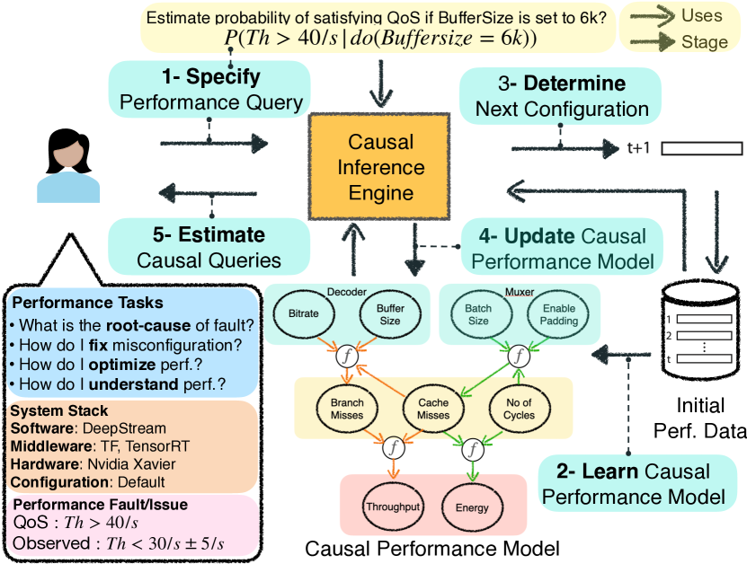
Figure 7. Overview of Unicorn.

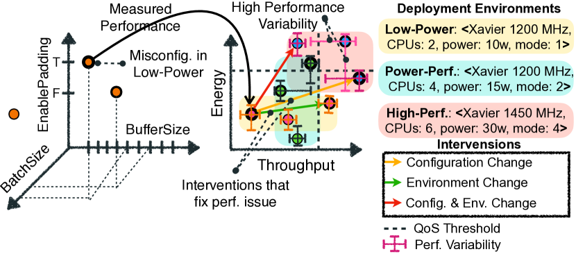
Figure 8. Mapping configuration space to multi-objective performance space.

Overview.

Unicorn works in five stages, implementing an active learning loop (cf. Fig. 7): (i) Users or developers of a highly-configurable system specify, in a human-readable language, the performance task at hand in terms of a query in the Inference Engine. For example, a Deepstream user may have experienced a throughput drop when they have deployed it on NVIDIA Xavier in low-power mode (cf. Fig. 8). Then, Unicorn’s main process starts by (ii) collecting some predetermined number of samples and learning a causal performance model; Here, a sample contains a system configuration and its corresponding measurement—including low-level system events and end-to-end system performance. Given a certain budget, which in practice either translates to time (iqbal2020flexibo) or several samples (jamshidi2016uncertainty), Unicorn, at each iteration, (iii) determines the next configuration(s) and measures system performance when deployed with the determined configuration–i.e. new sample; accordingly, (iv) the learned causal performance model is incrementally updated, reflecting a model that captures the underlying causal structure of the system performance. Unicorn terminates if either budget is exhausted or the same configuration has been selected a certain number of times consecutively, otherwise, it continues from Stage III. Finally, (v) to automatically derive the quantities which are needed to conduct the performance tasks, the specified performance queries are translated to formal causal queries, and they will be estimated based on the final causal model.

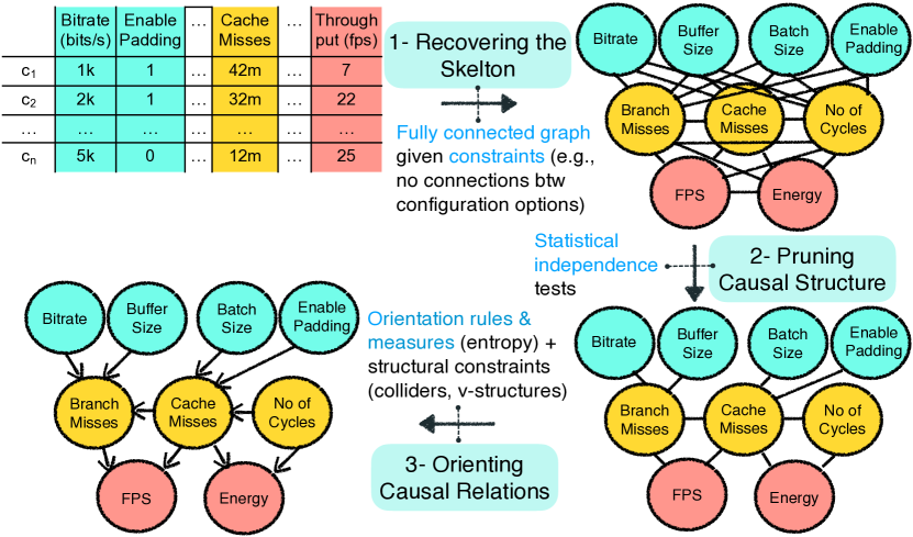
Figure 9. Causal model learning from performance data.

Stage I: Formulate Performance Queries.

Unicorn enables  developers and  users of highly-configurable systems to conduct performance tasks, including performance debugging, optimization, and tuning, n particular, when they need to answer several performance queries: (i) What configuration options caused the performance fault? (ii) What are important options and their interactions that influence performance? (iii) How to optimize one quality or navigate tradeoffs among multiple qualities in a reliable and explainable fashion? (iv) How can we understand what options and possible interactions are most responsible for the performance degradation in production?

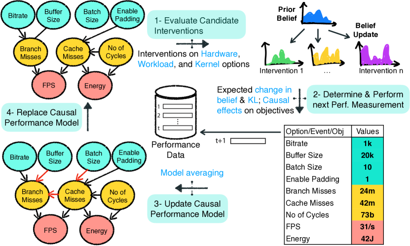
Figure 10. Causal model update.

At this stage, the performance queries are translated to formal causal queries using the interface of the causal inference engine (cf. Fig. 7). Note that in the current implementation of Unicorn, this translation is performed manually, however, this process could be made automated by creating a grammar for specifying performance queries and the translations can be made between the performance queries into the well-defined causal queries, note that such translation has been done in domains such as genomics (farahmand2019causal).

Stage II: Learn Causal Performance Model.

In this stage, Unicorn learns a causal performance model (see Section 2) that explains the causal relations between configuration options, the intermediate causal mechanism, and performance objectives. Here, we use an existing structure learning algorithm called Fast Causal Inference (hereafter, FCI) (spirtes2000causation). We selected FCI because: (i) it accommodates for the existence of unobserved confounders (spirtes2000causation; ogarrio2016hybrid; glymour2019review), i.e., it operates even when there are latent common causes that have not been, or cannot be, measured. This is important because we do not assume absolute knowledge about configuration space, hence there could be certain configurations we could not modify or system events we have not observed. (ii) FCI, also, accommodates variables that belong to various data types such as nominal, ordinal, and categorical data common across the system stack (cf. Fig. 8). To build the causal performance model, we, first, gather a set of initial samples (cf. Fig. 9). To ensure reliability (curtsinger2013stabilizer; ding2021generalizable), we measure each configuration multiple times, and we use the median (as an unbiased measure) for the causal model learning. As depicted in Fig. 9, Unicorn implements three steps for causal structure learning: (i) recovering the skeleton of the causal performance model by enforcing structural constraints; (ii) pruning the recovered structure using standard statistical tests of independence. In particular, we use mutual info for discrete variables and Fisher z-test for continuous variables; (iii) orienting undirected edges using entropy (spirtes2000causation; ogarrio2016hybrid; glymour2019review; colombo2012learning; colombo2014order).

Orienting undirected causal links. We orient undirected edges using prescribed edge orientation rules (spirtes2000causation; ogarrio2016hybrid; glymour2019review; colombo2012learning; colombo2014order) to produce a partial ancestral graph (or PAG). A PAG contains the following types of (partially) directed edges:

• $X$ $Y$ indicating that vertex $X$ causes $Y$.

• $X$ $Y$ which indicates that there are unmeasured confounders between vertices $X$ and $Y$.

In addition, a PAG produces two types of edges:

• $X$ $Y$ indicating that either $X$ causes $Y$, or that there are unmeasured confounders that cause both $X$ and $Y$.

• $X$  $Y$ which indicates that either: (a) vertices $X$ causes $Y$, or (b) vertex $Y$ causes $X$, or (c) there are unmeasured confounders that cause both $X$ and $Y$.

Figure 11. (a) The hamming distance between the learned causal model and ground truth model decreases as the algorithms measure more configuration samples. Incremental update of (b) Latency and (c) Energy, using Unicorn for debugging a multi-objective fault. Configuration options selected by Unicorn at each iteration are during debugging are shown in (d) using the yellow-colored nodes. Red-colored nodes indicate configuration options that are selected as a fix to the multi-objective performance fault. Mapping between option indexes and configuration options are shown in the supplementary materials.

In the last two cases, the circle ($\circ$) indicates that there is an ambiguity in the edge type. In other words, given the current observational data, the circle can indicate an arrowhead ( ) or no arrowhead (—), i.e., for $X$ $Y$, all three of $X$ $Y$, $Y$ $X$, and $X$ $Y$ might be compatible with current data, i.e., the current data could be faithful to each of these statistically equivalent causal graphs inducing the same conditional independence relationships.

Resolving partially directed edges.  For subsequent analyses over the causal graph, the PAG obtained must be fully resolved (directed with no $\circ$ ended edges) in order to generate an ADMG. We use the information-theoretic approach using entropy proposed in (Kocaoglu2017; Kocaoglu2020) to discover the true causal direction between two variables. Our work extends the theoretic underpinnings of entropic causal discovery to generate a fully directed causal graph by resolving the partially directed edges produced by FCI. For each partially directed edge, we follow two steps: (i) establish if we can generate a latent variable (with low entropy) to serve as a common cause between two vertices; (ii) if such a latent variable does not exist, then pick the direction which has the lowest entropy.

For the first step, we assess if there could be an unmeasured confounder (say $Z$) that lies between two partially oriented nodes (say $X$ and $Y$). For this, we use the LatentSearch algorithm proposed by Kocaoglu et al. (Kocaoglu2020). LatentSearch outputs a joint distribution $q(X,Y,Z)$ of the variables $X$, $Y$, and $Z$ which can be used to compute the entropy $H(Z)$ of the unmeasured confounder $Z$. Following the guidelines of Kocaoglu et al., we set an entropy threshold $\theta_{r}=0.8\times min\left\{H(X),H(Y)\right\}$. If the entropy $H(Z)$ of the unmeasured confounder falls below this threshold, then we declare that there is a simple unmeasured confounder $Z$ (with a low enough entropy) to serve as a common cause between $X$ and $Y$ and accordingly, we replace the partial edge with a bidirected (i.e., ) edge.

When there is no latent variable with a sufficiently low entropy, two possibilities exist: (i) variable $X$ causes $Y$; then, there is an arbitrary function $f(\cdot)$ such that $Y=f(X,E)$, where $E$ is an exogenous variable (independent of $X$) that accounts for system noise; or (ii) variable $Y$ causes $X$; then, there is an arbitrary function $g(\cdot)$ such that $X=g(Y,\tilde{E})$, where $\tilde{E}$ is an exogenous variable (independent of $Y$) that accounts for noise in the system. The distribution of $E$ and $\tilde{E}$ can be inferred from the data (Kocaoglu2017, see §3.1). With these distributions, we measure the entropies $H(E)$ and $H(\tilde{E})$. If $H(E)<H(\tilde{E})$, then, it is simpler to explain the $X$ $Y$ (i.e., the entropy is lower when $Y=f(X,E)$) and we choose $X$ $Y$. Otherwise, we choose $Y$ $X$.

2 Problem (code_transplant:online): For a real-time scene detection task, TX2 (faster platform) only processed 4 frames/sec whereas TX1 (slower platform) processed 17 frames/sec, i.e., the latency is $4\times$ worse on TX2.

Observed Latency (frames/sec): 4 FPS

Expected Latency (frames/sec): 22-24 FPS (30-40% better)

2

2-62.5   Configuration Options	Unicorn	SMAC	BugDoc	Forum	ACE${}^{\dagger}$    [t]
2-62.5
2.5   CPU Cores					3%    [t]
CPU Frequency					6%
EMC Frequency					13%
GPU Frequency					22%
Scheduler Policy	$\cdot$			$\cdot$	.
kernel.sched_rt_runtime_us	$\cdot$	$\cdot$		$\cdot$	.
kernel.sched_child_runs_first	$\cdot$	$\cdot$		$\cdot$	.
vm.dirty_background_ratio	$\cdot$	$\cdot$	$\cdot$	$\cdot$	.
vm.dirty_ratio	$\cdot$	$\cdot$		$\cdot$	.
Drop Caches	$\cdot$			$\cdot$	.
CUDA_STATIC					55%
vm.vfs_cache_pressure	$\cdot$	$\cdot$	$\cdot$	$\cdot$	.
vm.swappiness	$\cdot$			$\cdot$	1%
2.5
1-52.5   Latency (TX2 frames/sec)	28	24	21	23	[t]
Latency Gain (over TX1)	65%	41%	24%	35%
Latency Gain (over default)	7$\times$	6$\times$	5.25$\times$	5.75$\times$
Resolution time	22 mins	4 hrs	4 hrs	2 days
1-52.5

Figure 12. Using Unicorn on a real-world performance issue.

Stage III: Iterative Sampling (Active Learning).

At this stage, Unicorn determines the next configuration to be measured. Unicorn first estimates the causal effects of configuration options towards performance objectives using the learned causal performance model. Then, Unicorn iteratively determines the next system configuration using the estimated causal effects as a heuristic. Specifically, Unicorn determines the value assignments for options with a probability that is determined proportionally based on their associated causal effects. The key intuition is that such changes in the options are more likely to have a larger effect on performance objectives, and therefore, we can learn more about the performance behavior of the system. Given the exponentially large configuration space and the fact that the span of performance variations is determined by a small percentage of configurations, if we had ignored such estimates for determining the change in configuration options, the next configurations would result in considerable variations in performance objectives comparing with the existing data. Therefore, measuring the next configuration would not provide additional information for the causal model.

We extract paths from the causal graph (referred to as causal paths) and rank them from highest to lowest based on their average causal effect on latency, and energy. Using path extraction and ranking, we reduce the complex causal graph into a few useful causal paths for further analyses. The configurations in this path are more likely to be associated with the root cause of the fault.

Extracting causal paths with backtracking. A causal path is a directed path originating from either the configuration options or the system event and terminating at a non-functional property (i.e., throughput and/or energy). To discover causal paths, we backtrack from the nodes corresponding to each non-functional property until we reach a node with no parents. If any intermediate node has more than one parent, then we create a path for each parent and continue backtracking on each parent.

Ranking causal paths.  A complex causal graph can result in many causal paths. It is not practical to reason over all possible paths, as it may lead to a combinatorial explosion. Therefore, we rank the paths in descending of their causal effect on each non-functional property. For further analysis, we use paths with the highest causal effect. To rank the paths, we measure the causal effect of changing the value of one node (say Batch Size or $X$) on its successor (say Cache Misses or $Z$) in the path (say Batch Size  Cache Misses FPS and Energy). We express this with the do-calculus (pearl2009causality) notation: $\mathbb{E}[Z~{}|~{}\mathit{do}(X=x)]$. This notation represents the expected value of $Z$ (Cache Misses) if we set the value of the node $X$ (Batch Size) to $x$. To compute the average causal effect (ACE) of $X\rightarrow Z$ (i.e., Batch Size Cache Misses), we find the average effect over all permissible values of $X$ (Batch Size), i.e., $\mathrm{ACE}\left(Z,X\right)=\frac{1}{N}\cdot\sum_{\forall a,b\in X}\mathbb{E}\left[Z~{}|~{}\mathit{do}\left(X=b\right)\right]~{}-~{}\mathbb{E}\left[Z~{}|~{}\mathit{do}\left(X=a\right)\right]$. Here $N$ represents the total number of values $X$ (Batch Size) can take. If changes in Batch Size result in a large change in Cache Misses, then $\mathrm{ACE}\left(Z,X\right)$ will be larger, indicating that Batch Size has a large causal effect on Cache Misses.