Evolution of Stellar Orbits Around Merging Massive Black-Hole Binary

Abstract

We study the long-term orbital evolution of stars around a merging massive or supermassive black-hole (BH) binary, taking into account the general relativistic effect induced by the BH spin. When the BH spin is significant compared to and misaligned with the binary orbital angular momentum, the orbital axis ($\hat{\bm{l}}$) of the circumbinary star can undergo significant evolution during the binary orbital decay driven by gravitational radiation. Including the spin effect of the primary (more massive) BH, we find that starting from nearly coplanar orbital orientations, the orbital axes $\hat{\bm{l}}$ of circumbinary stars preferentially evolve towards the spin direction after the merger of the BH binary, regardless of the initial BH spin orientation. Such alignment phenomenon, i.e., small final misalignment angle between $\hat{\bm{l}}$ and the spin axis of the remanent BH $\hat{\bm{S}}$, can be understood analytically using the principle of adiabatic invariance. For the BH binaries with extremely mass ratio ($m_{2}/m_{1}\lesssim 0.01$), $\hat{\bm{l}}$ may experience more complicated evolution as adiabatic invariance breaks down, but the trend of alignment still works reasonably well when the initial binary spin-orbit angle is relatively small. Our result suggests that the correlation between the orientations of stellar orbits and the spin axis of the central BH could provide a potential signature of the merger history of the massive BH.

1 Introduction

Massive black-hole (BH) binaries, with orbital separations $\lesssim 10$ pc, are natural products of galaxy mergers (e.g., Begelman et al., 1980; Milosavljević & Merritt, 2001; Milosavljević & Phinney, 2005; Escala et al., 2005; Mayer et al., 2007; Dotti et al., 2007; Cuadra et al., 2009; Chapon et al., 2013; Fragione, 2022). Significant observational efforts have been devoted to searching for such binaries, and a number of candidate systems have been detected using various techniques (e.g., Sillanpaa et al., 1988; Komossa et al., 2003, 2008; Rodriguez et al., 2006; Bianchi et al., 2008; Bogdanović et al., 2009; Boroson & Lauer, 2009; Dotti et al., 2009; Comerford et al., 2009; Green et al., 2010; Deane et al., 2014; Liu et al., 2014; Bansal et al., 2017; Comerford et al., 2018; De Rosa et al., 2019). These massive BH binaries (BHBs) are likely surrounded by stars (or compact objects) associated with the merging galaxies. Alternatively, the stars could form in a circumbinary disk or be captured by the disk from a nuclear star cluster (e.g., Tagawa et al., 2020, 2021). For sufficiently small orbit separations, the massive binary BHs experience orbital decay and eventually merge, producing low-frequency gravitational waves (GWs). How would the orbits of the circumbinary stars change?

The secular gravitational interaction between a central binary and a surrounding object dictates the long-term evolution the system. For a hierarchical triple (with the semi-major axis $a_{\rm out}$ of the outer orbit much larger than that of the inner orbit $a_{\rm in}$), the secular evolution equations for arbitrary orbital eccentricities and orientations can be derived using expansion in $a_{\rm in}/a_{\rm out}$ [see Ford et al. (2000) for the equations to the octupole order; more compact equations in the vector form can be found in Liu et al. (2015a); Petrovich (2015)]. Such systems may exhibit excitations/oscillations in eccentricities and inclinations in both the inner and outer orbits (e.g. the well-known Lidov-Kozai effect; von Zeipel, 1910; Lidov, 1962; Kozai, 1962; Naoz, 2016). In general, the evolution can be highly irregular when the octupole effects are significant. If the outer body has a negligible mass compared to the inner binary, the dynamics of the outer body becomes simpler and analytical results can be obtained (e.g., Farago & Laskar, 2010; Li et al., 2014). In particular, the inner eccentric binary can drive significant inclination evolution of the outer orbit (e.g., Zanazzi & Lai, 2018) and produce orbit flipping from extreme eccentricity excitation (e.g., Naoz et al., 2017). Vinson & Chiang (2018) carried out a systematic study of the (secular) restricted three-body problem by expanding the potential to the hexadecapolar order (see also Gallardo et al., 2012) and identified various secular resonances.

In this paper, we study the secular evolution of stellar orbits around an inner massive BHB undergoing GW-induced orbital decay. We are particularly interested in the case of inner massive BHBs with relatively small mass ratios, such that the spin of the primary BH may play an important role. To the Newtonian leading order, the (inner) massive BHB makes the (outer) stellar orbit precess around the inner binary. However, when the BH spin is significant compared to the (inner) binary orbital angular momentum, the inner orbit axis undergoes Lens-Thirring (LT) precession around the BH spin axis. Therefore, the angular momentum axis of the stellar orbit can also be affected by the LT precession in an indirective way. In several recent studies (Liu et al., 2019; Liu & Lai, 2020, 2022), we have shown that the GR effects induced by a spinning tertiary SMBH plays an important role in the evolution of an inner stellar-mass binary. Here, we extend our previous studies to the “inverse” secular problem, in which the tertiary is essentially a test mass. By evolving the inner massive BHB until merger, we seek to identify the correlation (or signature) between the distribution of the surrounding stellar orbits and the final spin orientation of the BHB merger remanent.

This paper is organized as follows. In Section 2, we review the essential GR effects in the “BHB$+$outer test particle” system and present the secular equations in Post-Newtonian (PN) theory. In section 3, we identify different dynamical behaviors of the outer orbit for different parameters of the system. We perform analytical calculations of the final spin-orbit misalignment angles using the principle of adiabatic invariance. In Sections 4 and 5, we explore the final configurations of the stellar orbits at different distances from the central BHB, considering a range of mass ratios of BHB, coplanar/inclined initial orientations and eccentricities of the stellar orbits. We summarize our main results in Section 6.

2 Evolution Equations

We first review the secular dynamics of massless particles around a massive binary. Consider a black-hole binary (BHB) with semimajor axis $a_{\mathrm{in}}$, eccentricity vector $\bm{e}_{\mathrm{in}}$, total mass $m_{12}\equiv m_{1}+m_{2}$ (where $m_{1}$ and $m_{2}$ are the individual masses) and reduced mass $\mu_{\mathrm{in}}\equiv m_{1}m_{2}/m_{12}$. The outer test particle moves around the BHB with semimajor axis $a_{\mathrm{out}}$, eccentricity $\bm{e}_{\mathrm{out}}$. The orbital angular momenta of two orbits are $\bm{L}_{\mathrm{in}}\equiv L_{\mathrm{in}}\hat{\bm{l}}_{\mathrm{in}}=\mu_{\mathrm{in}}\sqrt{Gm_{12}a_{\mathrm{in}}(1-e_{\mathrm{in}}^{2})}\hat{\bm{l}}_{\mathrm{in}}$ and $\bm{L}_{\mathrm{out}}\equiv L_{\mathrm{out}}\hat{\bm{l}}_{\mathrm{out}}$ (see Figure 1). Throughout the paper, for convenience of notation, we will frequently omit the subscript “$\mathrm{out}$” for the outer orbit. The evolution of the system is governed by the double-averaged (DA; averaging over both the inner and outer orbital periods) secular equations of motion.

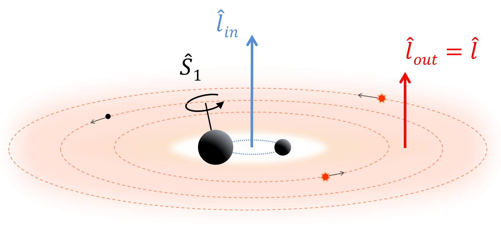
Figure 1: Schematic view of the set-up. We consider a massive BH binary at the center and a stellar disk around the binary. The inner orbit corresponds to the massive BH binary and has the unit vector of angular momentum $\hat{\bm{l}}_{\mathrm{in}}$. The primary component of the BH binary is assumed to be fast rotating with a spin unit vector ($\hat{\bm{S}}_{1}$). The outer stellar orbit is the test-particle orbit, which has the angular momentum unit vector $\hat{\bm{l}}_{\mathrm{out}}=\hat{\bm{l}}$.

For the inner binary, we set $e_{\mathrm{in}}=0$. The primary BH ($m_{1}$) in the binary has spin $\bm{S}_{1}=S_{1}\hat{\bm{S}}_{1}=(\chi_{1}Gm_{1}^{2}/c)\hat{\bm{S}}_{1}$, where $\chi_{1}\leqslant 1$ is the Kerr parameter. Throughout the paper, we assume $S_{2}\ll S_{1}$, thus neglecting the dynamical effect of the spin of the low-mass secondary ($m_{2}$); this approximation allows some of the dynamical spin-orbit behaviors to be understood analytically (see Section 3). However, all the equations showed below are valid for arbitrary mass ratio of the inner binary. The angular momentum $\bm{L}_{\mathrm{in}}$ evolves according to

$$\frac{d\bm{L}_{\mathrm{in}}}{dt}=\frac{d\bm{L}_{\mathrm{in}}}{dt}\bigg{|}_{\mathrm{GW}}+\frac{d\bm{L}_{\mathrm{in}}}{dt}\bigg{|}_{\mathrm{L_{\mathrm{in}}S}}~{},$$ (1)

where the two terms represent dissipation due to gravitational waves (GW) emission and the spin-orbit coupling, respectively. Gravitational radiation draws energy and angular momentum from the BH orbit, with (e.g., Peters, 1964)

$$\frac{d\bm{L}_{\mathrm{in}}}{dt}\bigg{|}_{\mathrm{GW}}=-\frac{32}{5}\frac{G^{3}}{c^{5}}\frac{\mu_{\mathrm{in}}m_{12}^{2}}{a_{\mathrm{in}}^{4}}\bm{L}_{\mathrm{in}}.$$ (2)

For reference, the merger time due to GW radiation of a binary with the initial semi-major axis $a_{\mathrm{in}}$ is given by

$$T_{\mathrm{m}} =\frac{5c^{5}a_{\mathrm{in}}^{4}}{256G^{3}m_{12}^{3}}\frac{(1+q)^{2}}{q}$$

$$\simeq 10^{10}\bigg{(}\frac{10^{6}M_{\odot}}{m_{12}}\bigg{)}^{3}\bigg{(}\frac{(1+q)^{2}/q}{12}\bigg{)}\bigg{(}\frac{a_{\mathrm{in}}}{224\mathrm{AU}}\bigg{)}^{4}\mathrm{yrs},$$

where we have introduced the mass ratio $q\equiv m_{2}/m_{1}$.

Spin-orbit coupling (1.5 PN effect) induces mutual precession of $\hat{\bm{L}}_{\mathrm{in}}$ around $\hat{\bm{S}}_{1}$ (e.g., Barker & O’Connell, 1975):

$$\frac{d\bm{L}_{\mathrm{in}}}{dt}\bigg{|}_{\mathrm{L_{\mathrm{in}}S}}=\Omega_{\mathrm{L_{\mathrm{in}}S}}\hat{\bm{S}}_{1}\times\bm{L}_{\mathrm{in}},$$ (4)

where

$$\Omega_{\mathrm{L_{\mathrm{in}}S}}=\frac{GS_{1}(4+3m_{2}/m_{1})}{2c^{2}a_{\mathrm{in}}^{3}}.$$ (5)

The spin vector $\bm{S}_{1}$ follows

$$\frac{d\bm{S}_{1}}{dt}=\Omega_{\mathrm{SL_{\mathrm{in}}}}\hat{\bm{l}}_{\mathrm{in}}\times\bm{S}_{1},$$ (6)

with

$$~{}~{}~{}\Omega_{\mathrm{SL_{\mathrm{in}}}}=\Omega_{\mathrm{L_{\mathrm{in}}S}}\frac{L_{\mathrm{in}}}{S_{1}}=\frac{3Gn_{\mathrm{in}}(m_{2}+\mu_{\mathrm{in}}/3)}{2c^{2}a_{\mathrm{in}}},$$ (7)

where $n_{\mathrm{in}}=(Gm_{12}/a_{\mathrm{in}}^{3})^{1/2}$ is the mean motion of the inner binary.

The time evolution equations of the outer orbital angular momentum axis $\hat{\bm{l}}$ and eccentricity $\bm{e}$ vectors are given by

$$\frac{d\hat{\bm{l}}}{dt}=\frac{d\hat{\bm{l}}}{dt}\bigg{|}_{\mathrm{L_{\mathrm{out}}L_{\mathrm{in}}}}^{\mathrm{(N)}}+\frac{d\hat{\bm{l}}}{dt}\bigg{|}_{\mathrm{L_{\mathrm{out}}L_{\mathrm{in}}}}^{\mathrm{(GR)}}+\frac{d\hat{\bm{l}}}{dt}\bigg{|}_{\mathrm{L_{\mathrm{out}}S}}~{},$$ (8)

$$\frac{d\bm{e}}{dt}=\frac{d\bm{e}}{dt}\bigg{|}_{\mathrm{L_{\mathrm{out}}L_{\mathrm{in}}}}^{\mathrm{(N)}}+\frac{d\bm{e}}{dt}\bigg{|}_{\mathrm{L_{\mathrm{out}}L_{\mathrm{in}}}}^{\mathrm{(GR)}}+\frac{d\bm{e}}{dt}\bigg{|}_{\mathrm{GR}}+\frac{d\bm{e}}{dt}\bigg{|}_{\mathrm{L_{\mathrm{out}}S}}~{}.$$ (9)

The precession of $\hat{\bm{l}}$ around $\hat{\bm{l}}_{\mathrm{in}}$ includes the Newtonian and GR components. The Newtonian precession can be described in the quadruple order

$$\frac{d\hat{\bm{l}}}{dt}\bigg{|}_{\mathrm{L_{\mathrm{out}}L_{\mathrm{in}}}}^{\mathrm{(N)}}=-\Omega_{\mathrm{out}}^{\mathrm{(N)}}(\hat{\bm{l}}_{\mathrm{in}}\cdot\hat{\bm{l}})\hat{\bm{l}}_{\mathrm{in}}\times\hat{\bm{l}},$$ (10)

with

$$\Omega_{\mathrm{out}}^{\mathrm{(N)}}=\frac{3}{4}\frac{\mu_{\mathrm{in}}a_{\mathrm{in}}^{2}}{m_{12}a^{2}}\frac{n}{(1-e^{2})^{2}},$$ (11)

where $n=(Gm_{12}/a^{3})^{1/2}$. Note that since $e_{\mathrm{in}}=0$, the high order Newtonian perturbation acting on the outer orbit can be ignored. Similarly,

$$\frac{d\bm{e}}{dt}\bigg{|}_{\mathrm{L_{\mathrm{out}}L_{\mathrm{in}}}}^{\mathrm{(N)}}=-\Omega_{\mathrm{out}}^{\mathrm{(N)}}\bigg{\{}(\hat{\bm{l}}_{\mathrm{in}}\cdot\hat{\bm{l}})\hat{\bm{l}}_{\mathrm{in}}\times\bm{e}-\Big{[}\frac{1}{2}-\frac{5}{2}(\hat{\bm{l}}_{\mathrm{in}}\cdot\hat{\bm{l}})^{2}\Big{]}\hat{\bm{l}}\times\bm{e}\bigg{\}}.$$ (12)

The GR components are given by (e.g., Liu et al., 2019; Liu & Lai, 2020)

$$\frac{d\hat{\bm{l}}}{dt}\bigg{|}_{\mathrm{L_{\mathrm{out}}L_{\mathrm{in}}}}^{(\mathrm{GR})}= \Omega_{\mathrm{out}}^{(\mathrm{GR})}\hat{\bm{l}}_{\mathrm{in}}\times\hat{\bm{l}},$$ (13)

$$\frac{d\bm{e}}{dt}\bigg{|}_{\mathrm{L_{\mathrm{out}}L_{\mathrm{in}}}}^{(\mathrm{GR})}= \Omega_{\mathrm{out}}^{(\mathrm{GR})}\hat{\bm{l}}_{\mathrm{in}}\times\bm{e}-3\Omega_{\mathrm{out}}^{(\mathrm{GR})}(\hat{\bm{l}}_{\mathrm{in}}\cdot\hat{\bm{l}})\hat{\bm{l}}\times\bm{e},$$ (14)

with

$$\Omega_{\mathrm{out}}^{(\mathrm{GR})}=\frac{2G\mu_{\mathrm{in}}n}{c^{2}}\sqrt{\frac{a_{\mathrm{in}}}{a^{3}(1-e^{2})^{3}}}.$$ (15)

GR (1-PN correction) introduces pericenter precession of the outer binary,

$$\frac{d\bm{e}}{dt}\bigg{|}_{\mathrm{GR}}=\Omega_{\mathrm{GR,out}}\hat{\bm{l}}\times\bm{e},$$ (16)

with

$$\Omega_{\mathrm{GR,out}}=3n\frac{Gm_{12}}{ac^{2}(1-e^{2})}.$$ (17)

Finally, the spin-orbit coupling also induces the precession of $\hat{\bm{l}}$ around $\bm{S}_{1}$:

$$\frac{d\hat{\bm{l}}}{dt}\bigg{|}_{\mathrm{L_{\mathrm{out}}S}} =\Omega_{\mathrm{L_{\mathrm{out}}S}}\hat{\bm{S}}_{1}\times\hat{\bm{l}},$$ (18)

$$\frac{d\bm{e}}{dt}\bigg{|}_{\mathrm{L_{\mathrm{out}}S}} =\Omega_{\mathrm{L_{\mathrm{out}}S}}\hat{\bm{S}}_{1}\times\bm{e}-3\Omega_{\mathrm{L_{\mathrm{out}}S}}\big{(}\hat{\bm{l}}\cdot\hat{\bm{S}}_{1}\big{)}\hat{\bm{l}}\times\bm{e},$$ (19)

where

$$\Omega_{\mathrm{L_{\mathrm{out}}S}}=\frac{2GS_{1}}{c^{2}a^{3}(1-e^{2})^{3/2}}.$$ (20)

By comparing Equations (15) and (20), we find that $\Omega_{\mathrm{L_{\mathrm{out}}S}}/\Omega_{\mathrm{out}}^{(\mathrm{GR})}=S_{1}/L_{\mathrm{in}}$(at $e_{\mathrm{in}}=0$).

3 Analytical Results

3.1 Different types of $\hat{\bm{l}}$ behaviors

To develop an analytic understanding of the dynamics, we assume the outer test particle has a circular orbit. If we define $\bm{J}\equiv J\hat{\bm{J}}=\bm{L}_{\mathrm{in}}+\bm{S}_{1}$, Equation (4) gives

$$\frac{d\hat{\bm{l}}_{\mathrm{in}}}{dt}\bigg{|}_{\mathrm{L_{\mathrm{in}}S}}=\frac{d\hat{\bm{l}}_{\mathrm{in}}}{dt}\bigg{|}_{\mathrm{L_{\mathrm{in}}J}}=\Omega_{\mathrm{in}}\hat{\bm{J}}\times\hat{\bm{l}}_{\mathrm{in}},$$ (21)

with

$$\Omega_{\mathrm{in}}=\Omega_{\mathrm{L_{\mathrm{in}}S}}\frac{J}{S_{1}}=\frac{GJ(4+3m_{2}/m_{1})}{2c^{2}a_{\mathrm{in}}^{3}}.$$ (22)

Combining Equations (10), (13) and (18), we find that the orbital axis $\hat{\bm{l}}$ of the test particle evolves according to

$$\frac{d\hat{\bm{l}}}{dt}=-\Omega_{\mathrm{out}}^{\mathrm{(N)}}(\hat{\bm{l}}_{\mathrm{in}}\cdot\hat{\bm{l}})\hat{\bm{l}}_{\mathrm{in}}\times\bm{l}+\Omega_{\mathrm{out}}^{{}^{\prime}(\mathrm{GR})}\hat{\bm{J}}\times\hat{\bm{l}},$$ (23)

where

$$\Omega_{\mathrm{out}}^{{}^{\prime}(\mathrm{GR})}=\frac{\Omega_{\mathrm{out}}^{(\mathrm{GR})}J}{L_{\mathrm{in}}}.$$ (24)

In the absence of GW dissipation, $\hat{\bm{l}}_{\mathrm{in}}$ rotates around $\hat{\bm{J}}$ at a constant rate, $\Omega_{\mathrm{in}}$, so it is useful to consider the evolution of $\hat{\bm{l}}$ in the frame corotating with $\hat{\bm{l}}_{\mathrm{in}}$. Combining Equations (21) and (23), we have

$$\bigg{(}\frac{d\hat{\bm{l}}}{dt}\bigg{)}_{\mathrm{rot}}=\bigg{[}-\Omega_{\mathrm{out}}^{\mathrm{(N)}}(\hat{\bm{l}}_{\mathrm{in}}\cdot\hat{\bm{l}})\hat{\bm{l}}_{\mathrm{in}}+(\Omega_{\mathrm{out}}^{{}^{\prime}(\mathrm{GR})}-\Omega_{\mathrm{in}})\hat{\bm{J}}\bigg{]}\times\hat{\bm{l}}.$$ (25)

The corresponding Hamiltonian can be given by

$$\mathcal{H}=-\frac{1}{2}\Omega_{\mathrm{out}}^{(\mathrm{N})}(\hat{\bm{l}}_{\mathrm{in}}\cdot\hat{\bm{l}})^{2}+(\Omega_{\mathrm{out}}^{{}^{\prime}(\mathrm{GR})}-\Omega_{\mathrm{in}})(\hat{\bm{J}}\cdot\hat{\bm{l}}).$$ (26)

We define the dimensionless Hamiltonian

$$\bar{\mathcal{H}}=\frac{\mathcal{H}}{\Omega_{\mathrm{out}}^{(\mathrm{N})}}=-\frac{1}{2}(\hat{\bm{l}}_{\mathrm{in}}\cdot\hat{\bm{l}})^{2}+\bigg{(}\lambda\frac{J}{L_{\mathrm{in}}}-\eta\bigg{)}(\hat{\bm{J}}\cdot\hat{\bm{l}}),$$ (27)

where we have introduced the dimensionless ratios

$$\lambda=\frac{\Omega_{\mathrm{out}}^{{}^{\prime}(\mathrm{GR})}}{\Omega_{\mathrm{out}}^{(\mathrm{N})}},~{}~{}~{}\eta=\frac{\Omega_{\mathrm{in}}}{\Omega_{\mathrm{out}}^{(\mathrm{N})}}.$$ (28)

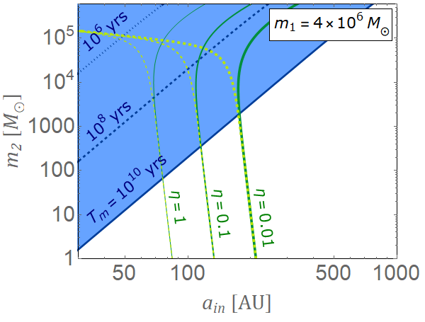
Figure 2: Parameter space in the $m_{2}$-$a_{\mathrm{in}}$ plane. The primary BH has mass $m_{1}=4\times 10^{6}M_{\odot}$, and the orbits are assumed to be circular. The blue region corresponds to the BHB that can merge within $10^{10}$yrs, and the dark blue solid, dashed, dotted lines are evaluated at $T_{\mathrm{m}}=10^{10}$, $10^{8}$ and $10^{6}$ yrs (Equation 2), respectively. The Green lines show different values of $\eta$ (see Equation 28) evaluated for $a=a_{\mathrm{out}}=a_{\mathrm{out},\mathrm{c}}$ (see Equation 3.1). The solid/dashed lines are the results of $\theta_{\mathrm{S},\mathrm{in}}=0^{\circ},180^{\circ}$.

Note that compared to the Newtonian precession $(\Omega_{\mathrm{out}}^{(\mathrm{N})})$, the GR precession $(\Omega_{\mathrm{out}}^{{}^{\prime}(\mathrm{GR})})$ of $\hat{\bm{l}}$ is only important near the merger of the inner binary. We thus ignore the $\lambda$ term in our analytical analysis. Depending on the value of $\eta$, we expect three possible $\hat{\bm{l}}$ behaviors: (i) For $\eta\ll 1$, $\hat{\bm{l}}$ closely follows $\hat{\bm{l}}_{\mathrm{in}}$, maintaining an approximately constant $I=\cos^{-1}(\hat{\bm{l}}_{\mathrm{in}}\cdot\hat{\bm{l}})$. (ii) For $\eta\gg 1$, $\hat{\bm{l}}$ effectively precesses around $\hat{\bm{J}}$ with approximately constant $\theta=\cos^{-1}(\hat{\bm{l}}\cdot\hat{\bm{J}})$. (iii) When $\eta\sim 1$, a resonance behavior of $\hat{\bm{l}}$ may occur, and large oscillation in $I$ can be generated.

Figure 2 presents the parameter space indicating the how the dynamical behavior of $\hat{\bm{l}}$ can change during the merger of the inner BHB. We set the primary component of the BHB to be $m_{1}=4\times 10^{6}M_{\odot}$, and vary the mass of the secondary component ($m_{2}$) and the semimajor axis of the BHB ($a_{\mathrm{in}}$). The contours of constant $\eta$ are evaluated for the closest stable test particle orbits around the binary (Holman & Wiegert, 1999):

$$a_{\mathrm{out},\mathrm{c}}=(1.6+5.1e-2.22e^{2}+4.12\mu_{\mathrm{c}}-4.27e\mu_{\mathrm{c}}$$

$$~{}~{}~{}~{}~{}~{}~{}~{}~{}~{}~{}-5.09\mu_{\mathrm{c}}^{2}+4.61e^{2}\mu_{\mathrm{c}}^{2})a_{\mathrm{in}},$$ (29)

where $\mu_{\mathrm{c}}=m_{2}/m_{12}$. We see that for a given $m_{2}$, as $a_{\mathrm{in}}$ decreases, $\eta$ increases and the outer orbit may experience three types dynamical behaviors successively.

To study such behaviors, we set up a coordinate system with $\hat{z}=\hat{\bm{l}}_{\mathrm{in}}$, $\hat{y}\sin\alpha\equiv\hat{\bm{l}}_{\mathrm{in}}\times\hat{\bm{J}}$, and let $\hat{\bm{l}}=\sin I(\cos\varphi\hat{x}+\sin\varphi\hat{y})+\cos I\hat{z}$, where $\alpha$ is the angle between $\hat{\bm{l}}_{\mathrm{in}}$ and $\hat{\bm{J}}$ (see panel (a) of Figure 3). Equation (27) becomes (neglecting the $\lambda$ term)

$$\bar{\mathcal{H}}=-\frac{1}{2}\cos^{2}I-\eta\Big{(}\cos\alpha\cos I+\sin\alpha\sin I\cos\varphi\Big{)}.$$ (30)

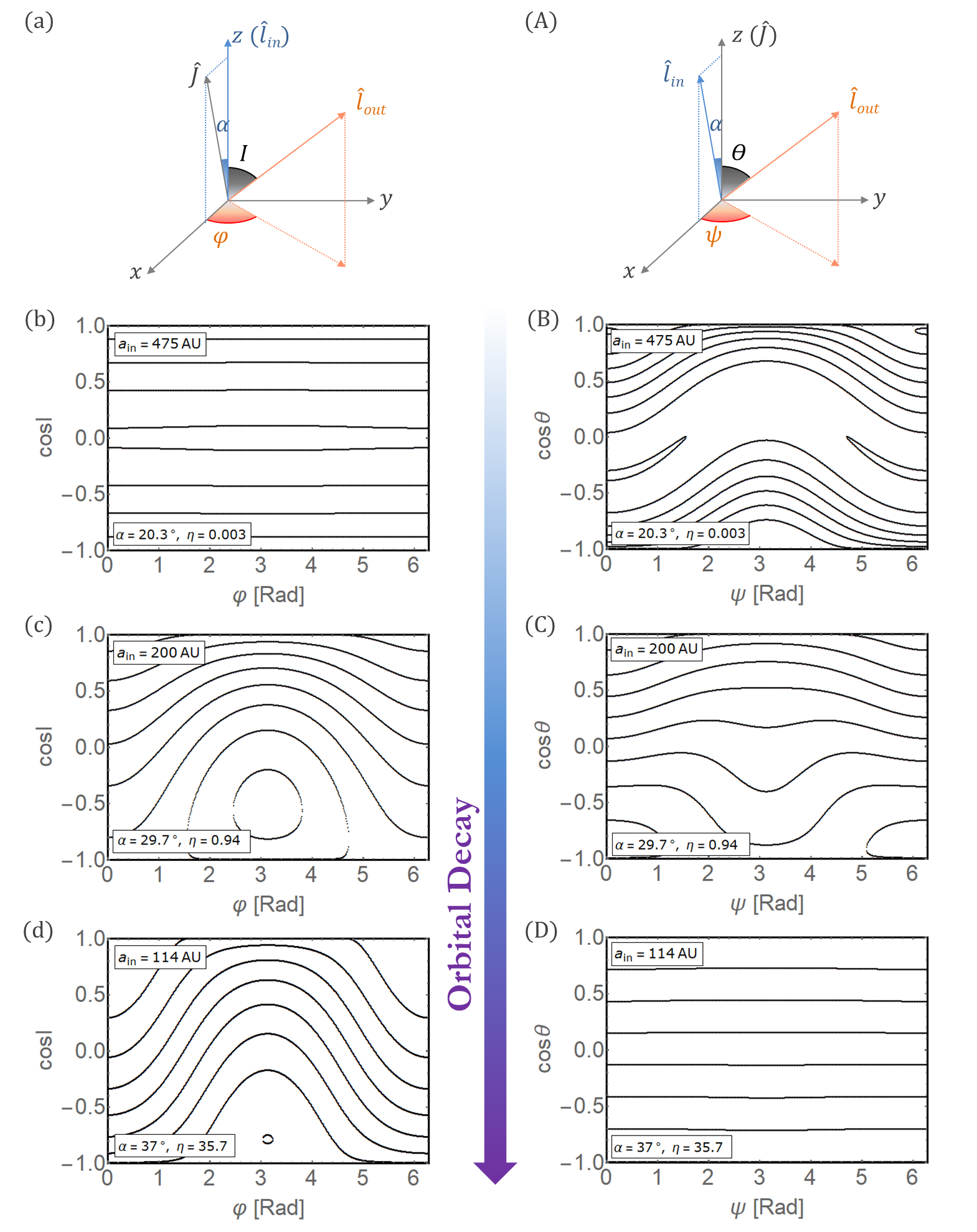
Figure 3: Different types of $\hat{\bm{l}}$ behaviors for three values of $a_{\mathrm{in}}$ (as labeled), representing the different stages of the orbital decay of the inner BHB. Panels (a) and (A) show the coordinate system used to describe the triple system, where $z-$axis is aligned with $\hat{\bm{l}}_{\mathrm{in}}$ and $\hat{\bm{J}}$, respectively. Panels (b)-(d) and (B)-(D) show the phase-space portraits with two different sets of canonical variables ($\cos I-\varphi$ and $\cos\theta-\psi$). The system parameters studied here are $m_{1}=4\times 10^{6}M_{\odot}$, $m_{2}=10^{5}M_{\odot}$, $a_{\mathrm{out}}=1000\mathrm{AU}$ and $e_{\mathrm{in}}=e_{\mathrm{out}}=0$. The solid lines shown in the panels (b)-(d) and (B)-(D) are contours of constant $\bar{\mathcal{H}}$ (see Equations 30 and 31), where we keep a constant $\theta_{\mathrm{S},\mathrm{in}}=90^{\circ}$ ($\theta_{\mathrm{S},\mathrm{in}}$ is the angle between $\hat{\bm{l}}_{\mathrm{in}}$ and $\hat{\bm{S}}_{1}$).

Alternatively, we can also set up a coordinate system with $\hat{z}=\hat{\bm{J}}$, as shown in the panel (A) of Figure 3. In this case, we have

$$\bar{\mathcal{H}}=-\frac{1}{2}\Big{(}\cos\alpha\cos\theta+\sin\alpha\sin\theta\cos\psi\Big{)}^{2}-\eta\cos\theta.$$ (31)

Figure 3 shows the dynamical behaviors of $\hat{\bm{l}}=\hat{\bm{l}}_{\mathrm{out}}$ for different values of $a_{\mathrm{in}}$, representing different stages of the orbital decay of the BHB ($m_{1}=4\times 10^{6}M_{\odot}$, $m_{2}=10^{5}M_{\odot}$). For each $a_{\mathrm{in}}$, the evolution of $\hat{\bm{l}}$ follows the trajectory of constant $\bar{\mathcal{H}}$ (using Equations 30 or 31 with a fixed spin-orbit misalignment angle). Panels (b)-(d) and (B)-(D) show some example trajectories in the ($I,\varphi$) and ($\theta,\psi$) spaces. We see that in the early stage (when $a_{\mathrm{in}}=475$AU), $I$ is nearly constant (panel b) since $\eta\ll 1$; in the later stage ($a_{\mathrm{in}}=114$AU), $\theta$ becomes nearly constant since $\eta\gg 1$ (panel D). In between, both $I$ and $\theta$ can undergo oscillations (panels c and C). Thus, the outer angular momentum axis $\hat{\bm{l}}$ indeed shows three types behaviors as the inner BHB decays.

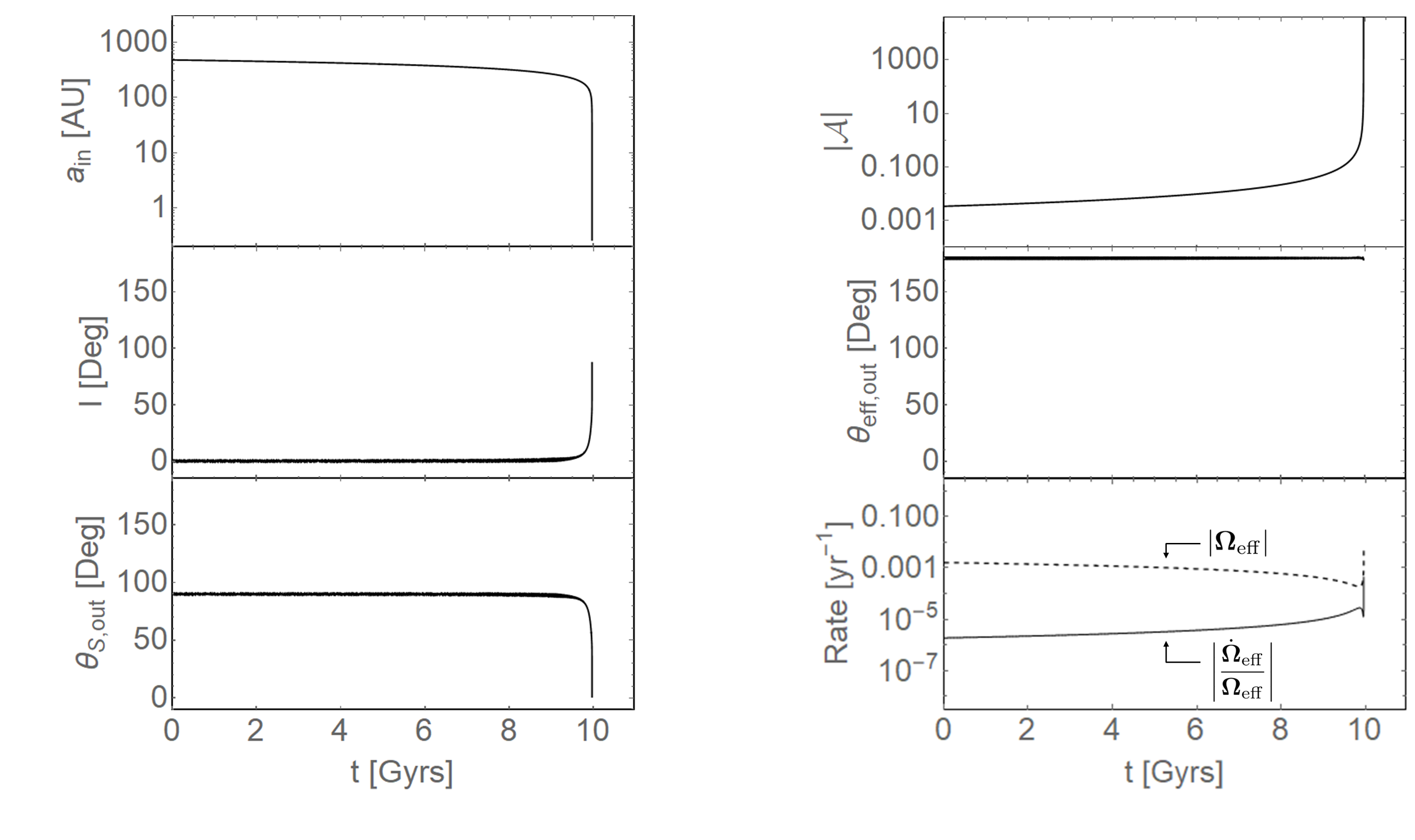
Figure 4: Evolution of an outer stellar orbit around an inner merging BHB, where the results are obtained by integrating Equations (1), (6), (8) and (9). The system parameters are $m_{1}=4\times 10^{6}M_{\odot}$, $m_{2}=10^{5}M_{\odot}$, $a_{\mathrm{out}}=1000\mathrm{AU}$, $e_{\mathrm{in}}=e_{\mathrm{out}}=0$ and the initial $a_{\mathrm{in}}=475\mathrm{AU}$, $I_{0}=0^{\circ}$. The primary component ($m_{1}$) has a misaligned spin at the initial moment, with $\theta_{\mathrm{S},\mathrm{in}}=90^{\circ}$. The left panels show the semimajor axis of the inner BHB ($a_{\mathrm{in}}$), inclination $I$ (the angle between $\hat{\bm{l}}_{\mathrm{in}}$ and $\hat{\bm{l}}$), and misalignment $\theta_{\mathrm{S},\mathrm{out}}$ (the angle between $\hat{\bm{S}}_{1}$ and $\hat{\bm{l}}$), and the right panels show the parameter $\mathcal{A}$ (Equation 32), $\theta_{\mathrm{eff},\mathrm{out}}$ (the angle between $\bm{\Omega}_{\mathrm{eff}}$ and $\hat{\bm{l}}$) and the relevant rates for evaluating adiabaticity (see Equation 34).

3.2 Final Spin-Orbit Misalignment Angles $\theta_{\mathrm{S},\mathrm{out}}^{\mathrm{f}}$

We now include GW dissipation of the BHB. We expect that after the merger, $\hat{\bm{J}}\rightarrow\hat{\bm{S}}_{1}$ and $\theta\rightarrow\theta_{\mathrm{S},\mathrm{out}}$.

Figure 4 shows an example of the evolution of $\hat{\bm{l}}$ during the orbital decay of BHB (with Equation 2 included in the calculation). In the top right panel, we introduce

$$\mathcal{A}=\frac{\Omega_{\mathrm{in}}}{\Omega_{\mathrm{out}}^{(\mathrm{N})}\cos I}=\frac{\eta}{\cos I}.$$ (32)

We see that the system goes through the transition from the “$\eta\ll 1$” regime to the “$\eta\gg 1$” regime. The orientation of $\hat{\bm{l}}$ varies a lot during the transition, and the initial alignment of $\hat{\bm{l}}_{\mathrm{in}}$ and $\hat{\bm{l}}$ is changed to the final alignment of $\hat{\bm{S}}_{1}$ and $\hat{\bm{l}}$.

The final spin-orbit misalignment ($\theta_{\mathrm{S},\mathrm{out}}^{\mathrm{f}}$) between $\hat{\bm{l}}$ and $\hat{\bm{S}}_{1}$ can be calculated analytically using the principle of adiabatic invariance, if the inner binary remains circular throughout the evolution. Equation (25) shows that $\bm{l}$ rotates around $\bm{\Omega}_{\mathrm{eff}}$, where

$$\bm{\Omega}_{\mathrm{eff}}=-\Omega_{\mathrm{out}}^{\mathrm{(N)}}(\hat{\bm{l}}_{\mathrm{in}}\cdot\hat{\bm{l}})\hat{\bm{l}}_{\mathrm{in}}-\Omega_{\mathrm{in}}\hat{\bm{J}}.$$ (33)

In the presence of GW dissipation, when the rate of change of $\bm{\Omega}_{\mathrm{eff}}$ is much smaller than $|\bm{\Omega}_{\mathrm{eff}}|$, i.e.,

$$\bigg{|}\frac{\dot{\bm{\Omega}}_{\mathrm{eff}}}{\bm{\Omega}_{\mathrm{eff}}}\bigg{|}\ll|\bm{\Omega}_{\mathrm{eff}}|$$ (34)

$\bm{\Omega}_{\mathrm{eff}}$ becomes a slowly changing vector, and the angle between $\bm{\Omega}_{\mathrm{eff}}$ and $\hat{\bm{l}}$ is expected to be an adiabatic invariant, i.e.,

$$\theta_{\mathrm{eff},\mathrm{out}}\simeq\mathrm{constant}\qquad({\rm adiabatic~{}invariant}).$$ (35)

After the inner binary has decayed, we have $|\Omega_{\mathrm{out}}^{\mathrm{(N)}}|\ll|\Omega_{\mathrm{in}}|$, and $\bm{\Omega}_{\mathrm{eff}}\simeq\Omega_{\mathrm{in}}\hat{\bm{J}}$. Therefore,

$$\theta_{\mathrm{S},\mathrm{out}}^{\mathrm{f}}\simeq\theta_{\mathrm{eff},\mathrm{out}}^{\mathrm{f}}=\theta_{\mathrm{eff},\mathrm{out}}^{0}.$$ (36)

To obtain $\theta_{\mathrm{eff},\mathrm{out}}^{0}$, we note that the orientation of the initial $\bm{\Omega}_{\mathrm{eff}}$ is determined by both $\hat{\bm{l}}_{\mathrm{in}}$ and $\hat{\bm{J}}$. For the outer orbits with $|\Omega_{\mathrm{out}}^{\mathrm{(N)}}|\gg|\Omega_{\mathrm{in}}|$ (generally corresponding to the systems with small $a_{\mathrm{out}}$), we have $\bm{\Omega}_{\mathrm{eff}}\simeq-\Omega_{\mathrm{out}}^{\mathrm{(N)}}\hat{\bm{l}}_{\mathrm{in}}$. As a result, the final spin-orbit misalignment angle is equal to the initial inclination angle between $\hat{\bm{l}}_{\mathrm{in}}$ and $\bm{l}$, i.e., $\theta_{\mathrm{S},\mathrm{out}}^{\mathrm{f}}\simeq\theta_{\mathrm{eff},\mathrm{out}}^{0}\simeq I_{0}$. For the example shown in Figure 4, we see that the adiabatic criterion (Equation 34) is satisfied and the adiabatic invariant $\theta_{\mathrm{eff},\mathrm{out}}$ is almost a constant. Since $\hat{\bm{l}}$ and $\hat{\bm{l}}_{\mathrm{in}}$ are initially aligned, $I_{0}=0$, the final spin-orbit misalignment angle $\theta_{\mathrm{S},\mathrm{out}}^{\mathrm{f}}=0$.

For the distant outer orbits, we have $|\Omega_{\mathrm{out}}^{\mathrm{(N)}}|\ll|\Omega_{\mathrm{in}}|$, and $\bm{\Omega}_{\mathrm{eff}}\simeq-\Omega_{\mathrm{in}}\hat{\bm{J}}$. Therefore, we expect that $\theta_{\mathrm{S},\mathrm{out}}^{\mathrm{f}}\simeq\theta_{\mathrm{eff},\mathrm{out}}^{0}\simeq\theta_{0}$, where $\theta_{0}$ is the angle between $\hat{\bm{J}}$ and $\hat{\bm{l}}$ at the initial moment. For the specific configuration with $I_{0}=0$, we have $\theta_{\mathrm{S},\mathrm{out}}^{\mathrm{f}}\simeq\alpha_{0}$, where $\alpha_{0}$ is the initial angle between $\hat{\bm{J}}$ and $\hat{\bm{l}}_{\mathrm{in}}$.

4 Results for Initially Coplanar Outer Orbits

4.1 Fiducial Case: $m_{2}=10^{5}M_{\odot}$

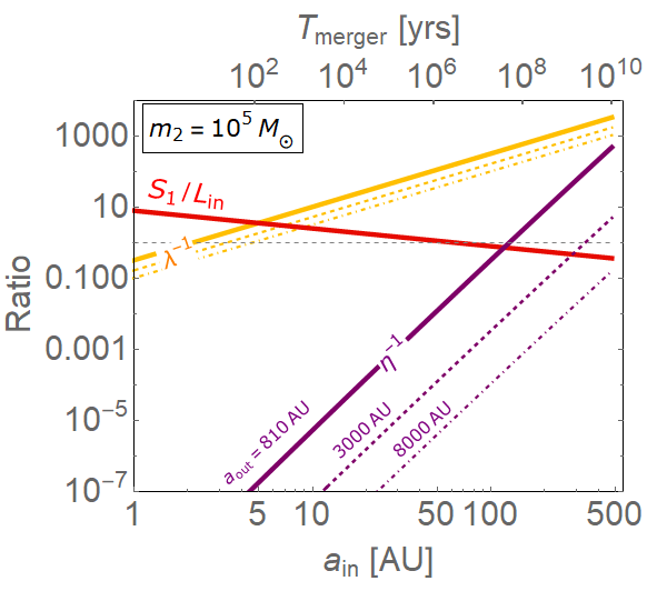
Figure 5: The variation of the values of $\eta$ and $\lambda$ as the inner BHB decays. The inner BHB has masses $m_{1}=4\times 10^{6}M_{\odot}$ and $m_{2}=10^{5}M_{\odot}$. The results (purple and orange lines) are obtained by using Equation (28) with $\theta_{\mathrm{S},\mathrm{in}}=0^{\circ}$, where the solid, dashed and dot-dashed lines are for the given $a_{\mathrm{out}}$ (as labeled; the minimum $a_{\mathrm{out}}$ is evaluated by Equation 3.1). We also show the ratio of $S_{1}/L_{\mathrm{in}}$ as a function of $a_{\mathrm{in}}$.

We now study the evolution of the outer orbits with different radius ($a_{\mathrm{out}}$) as the inner BHB decays. We consider the initially coplanar case with $I_{0}=0^{\circ}$ and $m_{2}=10^{5}M_{\odot}$ in this section.

Figure 5 shows $\lambda^{-1}$ and $\eta^{-1}$ (see Equation 28) as a function of $a_{\mathrm{in}}$ for a given $a_{\mathrm{out}}$. The values of $\eta$ are obtained by setting $\theta_{\mathrm{S},\mathrm{in}}=0^{\circ}$. We find that the nodal precession induced by GR ($\Omega_{\mathrm{out}}^{{}^{\prime}(\mathrm{GR})}$) is always weaker than the Newtonian one ($\Omega_{\mathrm{out}}^{(\mathrm{N})}$), until the inner BH binary has become sufficiently compact. On the other hand, when the BHB is wide, the systems, especially for the close test particle orbits (e.g., $a_{\mathrm{out}}=810\mathrm{AU}$), are in the “$\eta\gg 1$” regime, in which the Newtonian precession of $\hat{\bm{l}}$ around $\hat{\bm{l}}_{\mathrm{in}}$ is much stronger than the precession of $\hat{\bm{l}}_{\mathrm{in}}$ around $\hat{\bm{J}}$. This implies that the direction of $\bm{\Omega}_{\mathrm{eff}}$ is approximately parallel to $\hat{\bm{l}}_{\mathrm{in}}$ and $\theta_{\mathrm{eff},\mathrm{out}}^{0}\simeq I_{0}$. However, if the test particle is further away from the central BHB (i.e., $a_{\mathrm{out}}>3000\mathrm{AU}$), $\eta$ is close to unity and the orientation of $\bm{\Omega}_{\mathrm{eff}}$ is determined by both $\hat{\bm{l}}_{\mathrm{in}}$ and $\hat{\bm{J}}$.

In Figure 6, panel (A) shows the final spin-orbit angles $\theta_{\mathrm{S},\mathrm{out}}^{\mathrm{f}}$ for a series of test particle orbits with different separations, for several values of $\theta_{\mathrm{S},\mathrm{in}}^{0}$. We obtain the numerical results (dots) by integrating Equations (1), (6), (8) and (9) and the analytical results based on Equation (36). We find that the analytic prediction (dashed lines) agrees well with the numerical results. For the close test particle orbits, the final angular momentum $\hat{\bm{l}}$ always points in the direction of the spin $\hat{\bm{S}}_{1}$, i.e., $\theta_{\mathrm{S},\mathrm{out}}^{\mathrm{f}}\simeq I_{0}=0^{\circ}$, regardless of the initial spin orientation. This is because $\bm{\Omega}_{\mathrm{eff}}\varpropto\hat{\bm{l}}_{\mathrm{in}}$ for the orbits with $a_{\mathrm{out}}\lesssim 3000\mathrm{AU}$ (as shown in Figure 5). On the other hand, for $a_{\mathrm{out}}\gtrsim 3000\mathrm{AU}$, the final angle $\theta_{\mathrm{S},\mathrm{out}}^{\mathrm{f}}$ is only determined by $\theta_{\mathrm{eff},\mathrm{out}}^{0}$, and $\theta_{\mathrm{S},\mathrm{out}}^{\mathrm{f}}\simeq\alpha_{0}$ (the angle between $\hat{\bm{J}}$ and $\hat{\bm{l}}_{\mathrm{in}}$) as $a_{\mathrm{out}}\gtrsim 10^{4}\mathrm{AU}$. Since the initial orientation of $\bm{J}$ depends on $\theta_{\mathrm{S},\mathrm{in}}^{0}$, we see that the angles $\theta_{\mathrm{S},\mathrm{out}}^{\mathrm{f}}$ corresponding to different $\theta_{\mathrm{S},\mathrm{out}}^{\mathrm{f}}$ differ at large $a_{\mathrm{out}}$.

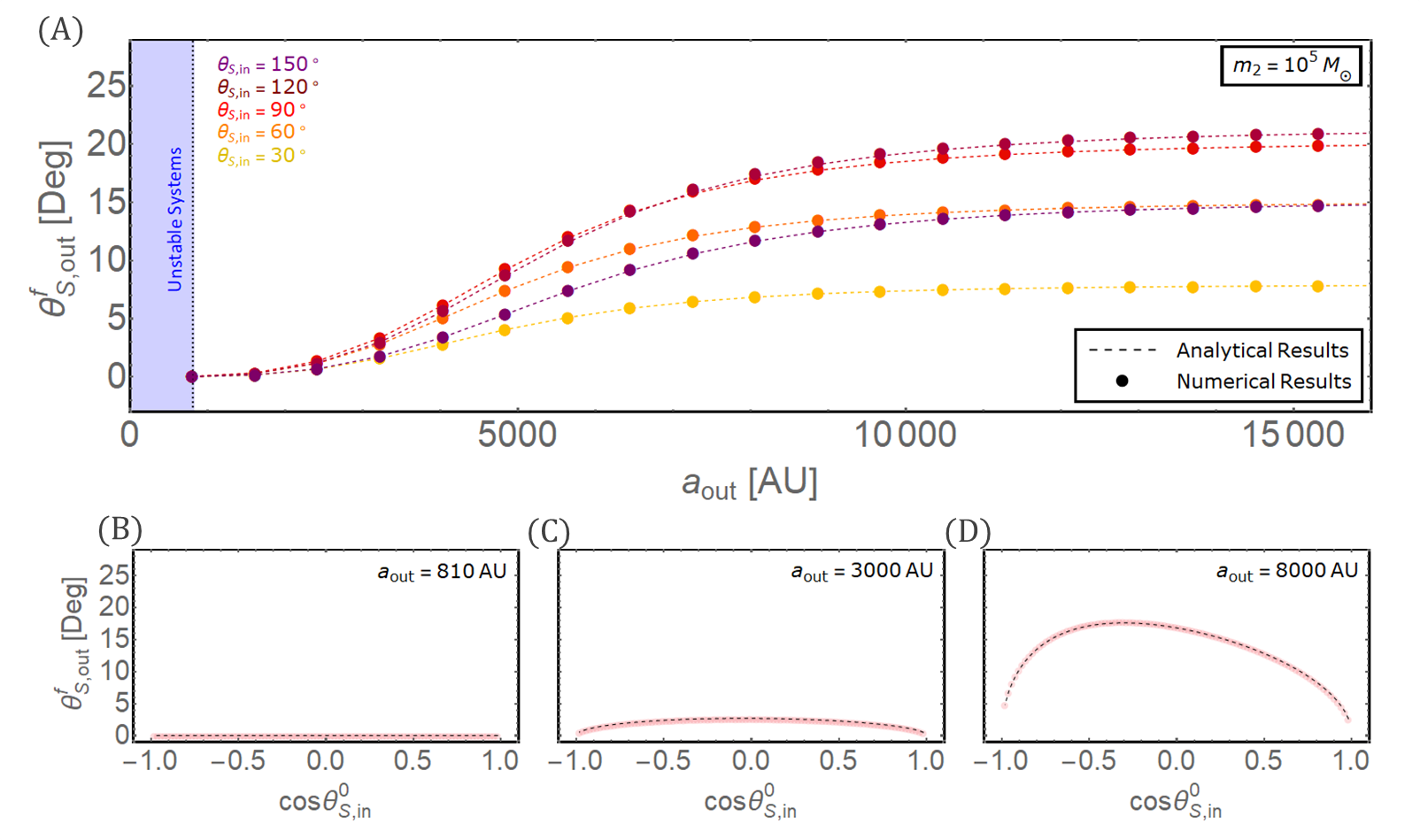
Figure 6: Panel (A) shows the final spin-orbit misalignment angles $\theta_{\mathrm{S},\mathrm{out}}^{\mathrm{f}}$ as a function of $a_{\mathrm{out}}$, for different initial spin orientations (as labeled). The system parameters follow the example shown in Figure 5. The stability criterion is given by Equation (3.1). All the dots are the numerical results obtained by integrating Equations (1), (6), (8) and (9). The dashed lines are the analytical results based on Equation (33). Panels (C)-(D) show the final angles $\theta_{\mathrm{S},\mathrm{out}}^{\mathrm{f}}$ as a function of a full range of $\cos\theta_{\mathrm{S},\mathrm{in}}^{0}$, with three values of $a_{\mathrm{out}}$. Again, the dots and the dashed lines are obtained numerically and analytically, respectively.

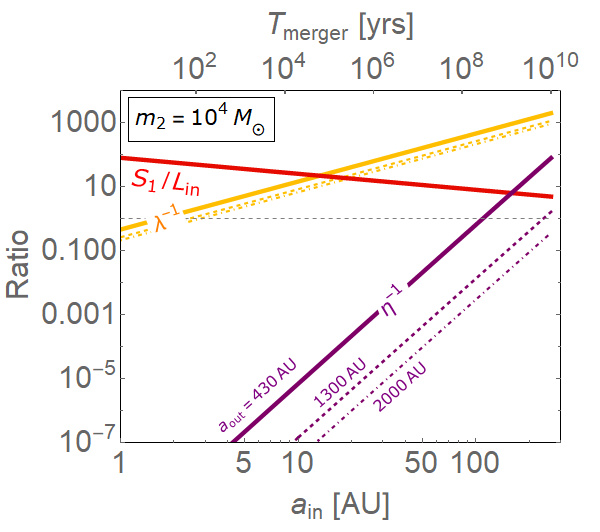
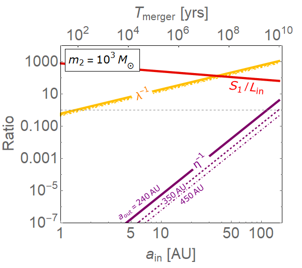
Figure 7: Same as Figure 5, except for $m_{2}=10^{4}M_{\odot}$ (left panel) and $m_{2}=10^{3}M_{\odot}$ (right panel).

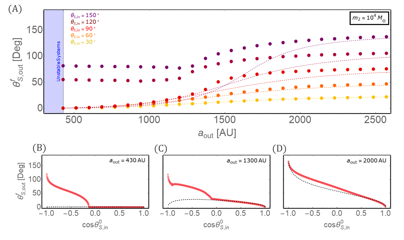
Figure 8: Same as Figure 6, except for $m_{2}=10^{4}M_{\odot}$.

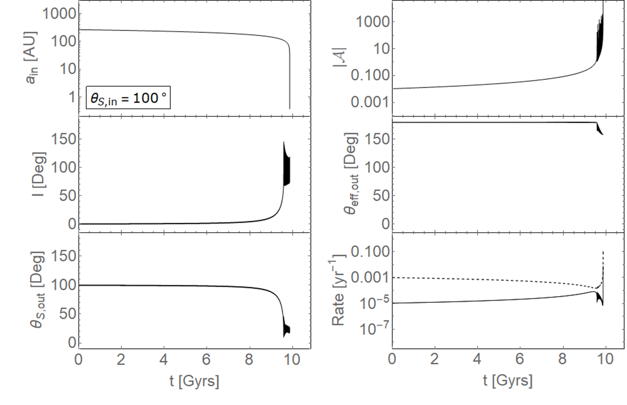
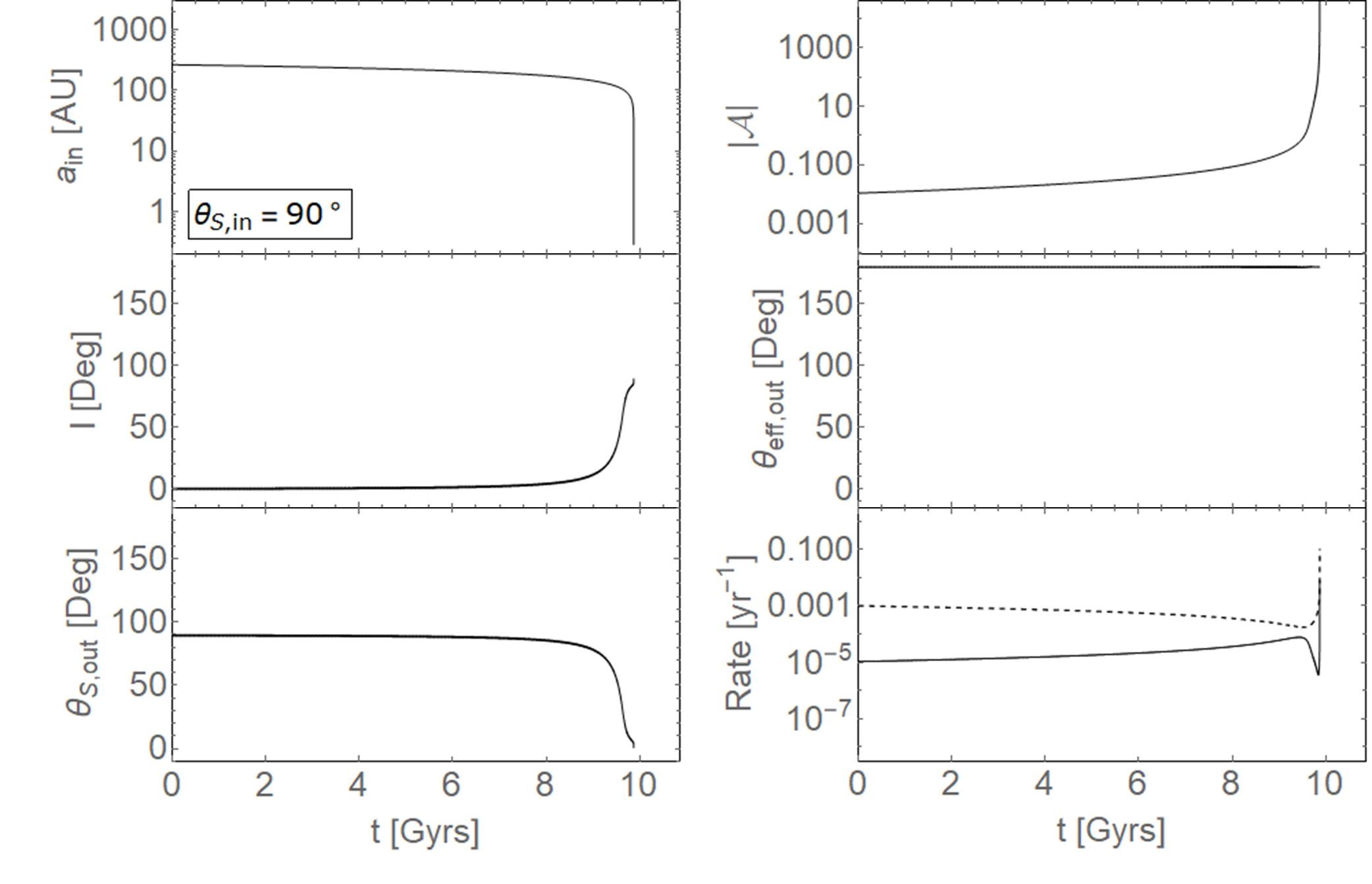
Figure 9: Similar to Figure 4, but the system parameters here are $m_{1}=4\times 10^{6}M_{\odot}$, $m_{2}=10^{4}M_{\odot}$, $a_{\mathrm{in}}=265\mathrm{AU}$, $a_{\mathrm{out}}=430\mathrm{AU}$, $e_{\mathrm{in}}=e_{\mathrm{out}}=0$ and $I_{0}=0^{\circ}$. We consider two values of $\theta_{\mathrm{S},\mathrm{in}}$ (as labeled) in the left and right panels.

Panels (B)-(D) of Figure 6 show the dependence of $\theta_{\mathrm{S},\mathrm{out}}^{\mathrm{f}}$ on $\theta_{\mathrm{S},\mathrm{in}}^{0}$ for three values of $a_{\mathrm{out}}$. We find that the analytical results are in excellent agreement with the numerical calculations.

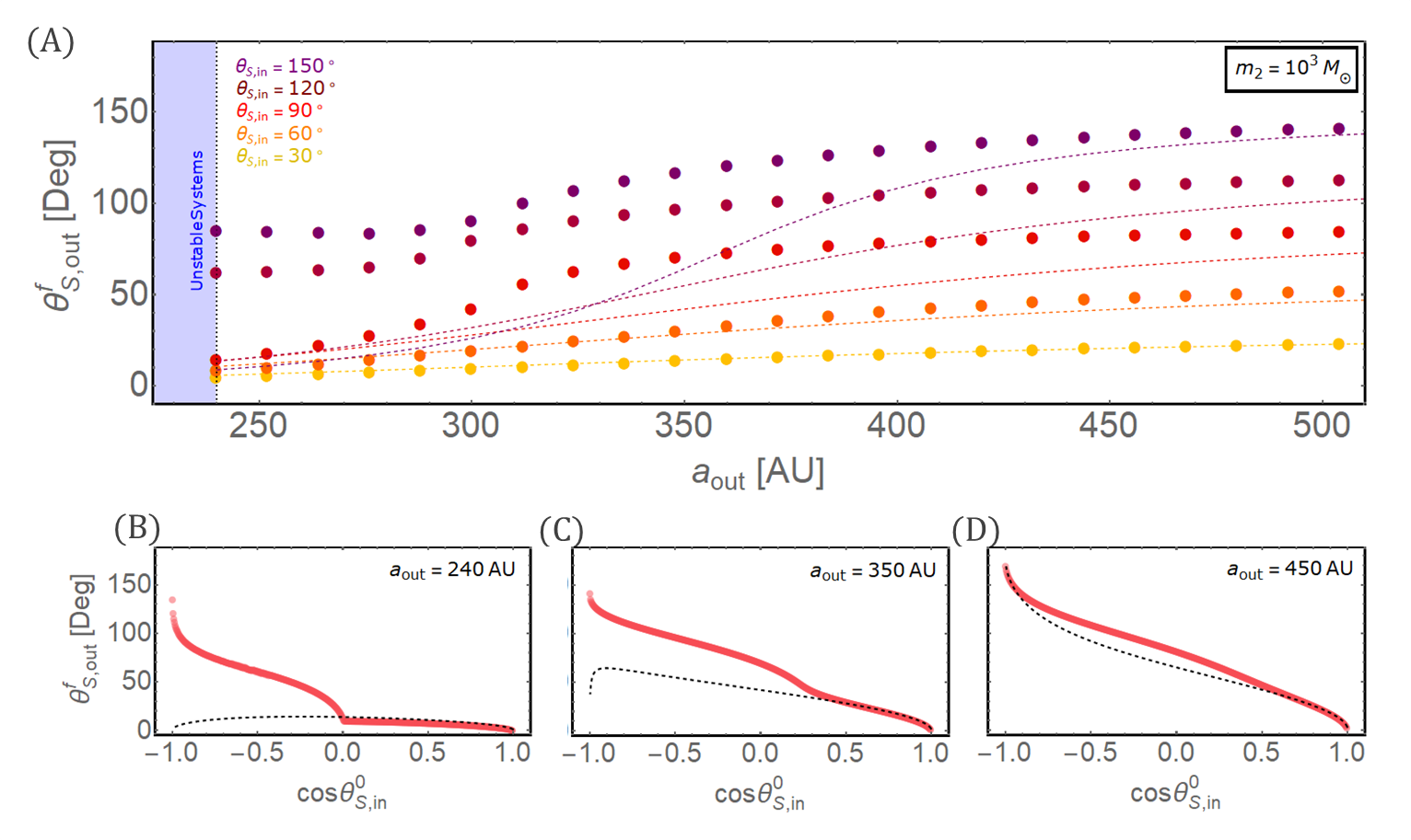
Figure 10: Same as Figure 6, except for $m_{2}=10^{3}M_{\odot}$.

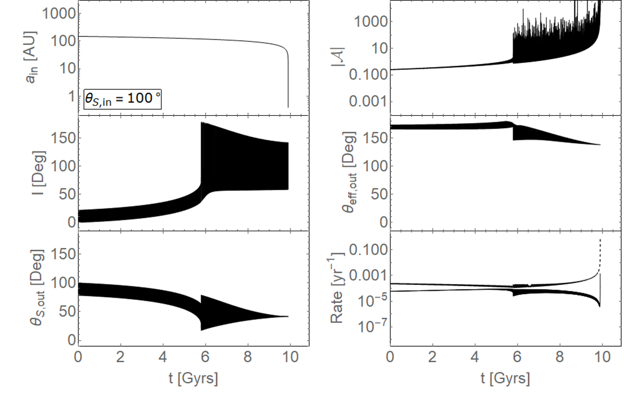
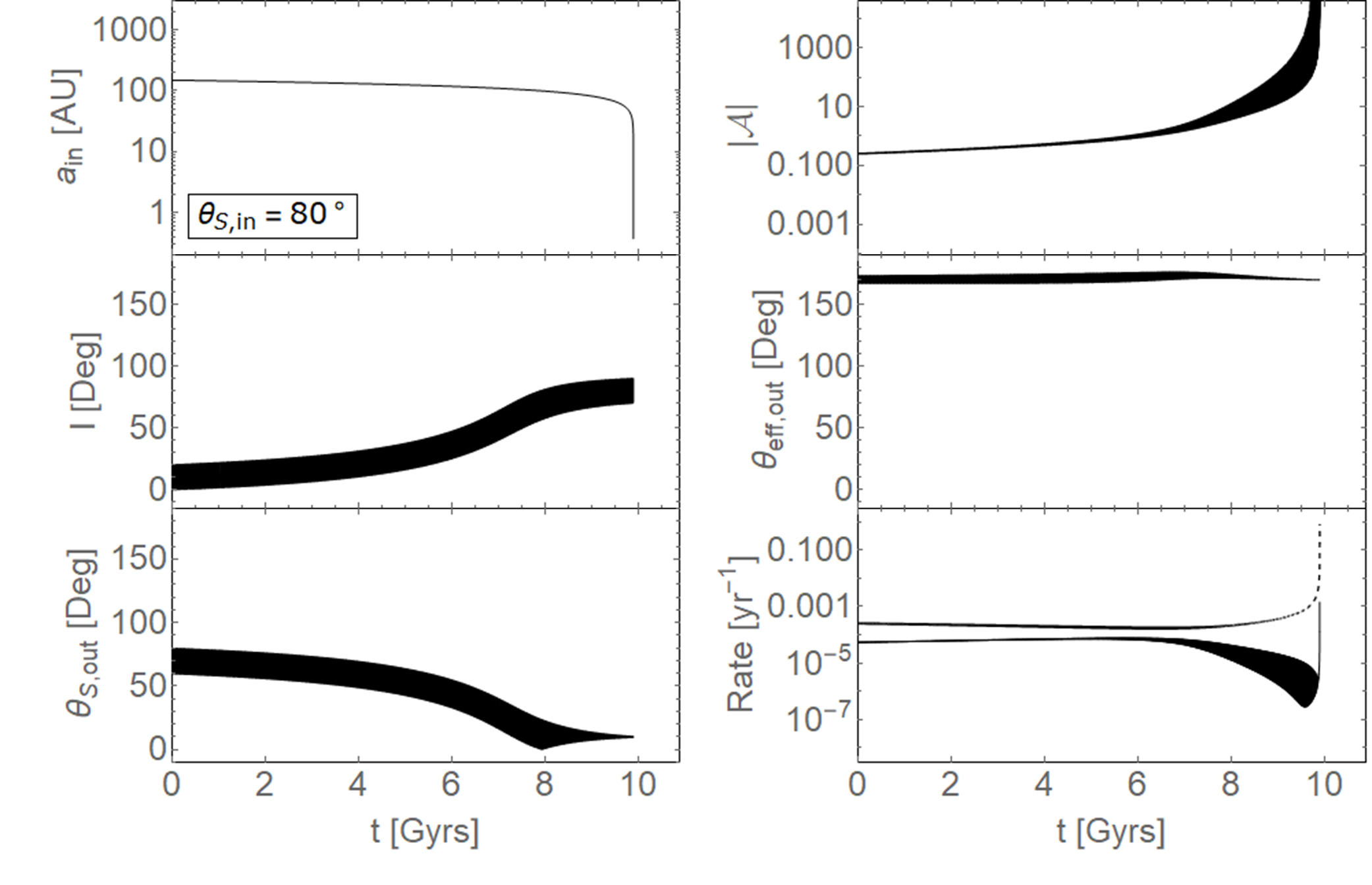
Figure 11: Similar to Figure 4, but the system parameters here are $m_{1}=4\times 10^{6}M_{\odot}$, $m_{2}=10^{3}M_{\odot}$, $a_{\mathrm{in}}=149\mathrm{AU}$, $a_{\mathrm{out}}=240\mathrm{AU}$, $e_{\mathrm{in}}=e_{\mathrm{out}}=0$ and $I_{0}=0^{\circ}$. We consider two values of $\theta_{\mathrm{S},\mathrm{in}}$ (as labeled) in the left and right panels.

4.2 $m_{2}=10^{4}M_{\odot}$ and $m_{2}=10^{3}M_{\odot}$

If $m_{2}$ becomes lighter, in order to have BHB merging within the Hubble timescale, $a_{\mathrm{in}}$ should be smaller (as shown in Figure 5). The initial systems maybe close to or even already in the “$\eta\sim 1$” regime, indicating that the angular momentum of the close test particle orbit $\hat{\bm{l}}$ may experience more complicated evolution at the early stage of the merger of the inner BHB.

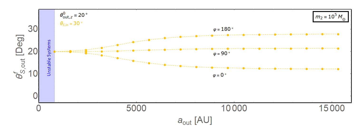
Figure 12: The final spin-orbit misalignment angle $\theta_{\mathrm{S},\mathrm{out}}^{\mathrm{f}}$ as a function of $a_{\mathrm{out}}$. The system parameters are $m_{1}=4\times 10^{6}M_{\odot}$, $m_{2}=10^{5}M_{\odot}$, $a_{\mathrm{in}}=475\mathrm{AU}$, and $e_{\mathrm{in}}=e_{\mathrm{out}}=0$. The primary component of BHB has a misaligned spin direction, with $\theta_{\mathrm{S},\mathrm{in}}^{0}=30^{\circ}$. The angular momentum of the outer orbit is initialized inclined with respect to the initial direction of $\hat{\bm{l}}_{\mathrm{in}}$ ($z-$axis; see also the panel (a) of Figure 3) by $20^{\circ}$ (i.e., $\theta_{\mathrm{out},\mathrm{z}}^{0}=20^{\circ}$), with three different phase angles ($\varphi=0^{\circ},90^{\circ},180^{\circ}$). The dots are from the numerical calculation and the dashed lines are the analytical results (i.e., $\theta_{\mathrm{S},\mathrm{out}}^{\mathrm{f}}=\theta_{\mathrm{eff},\mathrm{out}}^{0}$).

Figure 7 shows how $\lambda$ and $\eta$ change as $a_{\mathrm{in}}$ decreases when $m_{2}=10^{4}M_{\odot}$ (left panel) and $m_{2}=10^{3}M_{\odot}$ (right panel). Here, since $S_{1}\gg L_{\mathrm{in}}$, the orientation of $\hat{\bm{J}}$ is dominated by $\hat{\bm{S}}_{1}$.

Figure 8 shows the final angle $\theta_{\mathrm{S},\mathrm{out}}^{\mathrm{f}}$ as a function of $a_{\mathrm{out}}$ for a range of $\theta_{\mathrm{S},\mathrm{in}}^{0}$ values. Compared to the results shown in Figure 6, the analytical predictions are only valid for the small $\theta_{\mathrm{S},\mathrm{in}}^{0}$ or the the distant outer orbits (see also the panel D); for the test particle orbit with small $a_{\mathrm{out}}$, the analytical results break down when $\theta_{\mathrm{S},\mathrm{in}}^{0}\gtrsim 90^{\circ}$ (see also panels B and C).

Figure 9 shows two evolution examples for a system with small $a_{\mathrm{out}}$. We identify two main reasons for the discrepancy between the analytical and numerical results for $\theta_{\mathrm{S},\mathrm{out}}^{\mathrm{f}}$: (i) The time of entry into “$\eta\sim 1$” regime. The systems with small $m_{2}$ tend to have a relatively large $\eta$ ($\lesssim 1$), thus will enter the “$\eta\sim 1$” regime earlier. The inclination angle $I$ shown in Figure 9 has a chance to be excited (left panel) or experience oscillations (right panel) at earlier times compared to the example shown in Figure 4. Note that the exact value of $\eta$ depends on the choice of $\theta_{\mathrm{S},\mathrm{in}}^{0}$ (see Figure 2); (ii) Crossing $90^{\circ}$ in $I$. For the BHB with small mass ratio, the direction of $\hat{\bm{J}}$ is dominated by the spin vector $\hat{\bm{S}}_{1}$ instead of $\hat{\bm{l}}_{\mathrm{in}}$ (see Figure 7). Thus, for a given $\theta_{\mathrm{S},\mathrm{in}}^{0}$, the angle between $\hat{\bm{l}}_{\mathrm{in}}$ and $\hat{\bm{J}}$ (i.e., $\alpha$) is larger than the one for a BHB with comparable masses (e.g., Figure 5). The large $\alpha$ value may easily induce large inclinations ($I\gtrsim 90^{\circ}$) due to the precession of $\hat{\bm{l}}_{\mathrm{in}}$ around $\hat{\bm{J}}$ as the system reach the “$\eta\sim 1$” regime. Therefore, the crossing through $90^{\circ}$ in $I$ may occur and induces significant oscillations in $|\mathcal{A}|$ and $|\dot{\bm{\Omega}}_{\mathrm{eff}}|$, breaking the adiabaticity condition.

Figure 10 shows the results for $m_{2}=10^{3}M_{\odot}$. Similar to Figure 8, we find that the analytical results are in an agreement with the numerical calculations except when $a_{\mathrm{out}}$ is small ($a_{\mathrm{out}}\lesssim 400\mathrm{AU}$) and $\theta_{\mathrm{S},\mathrm{in}}^{0}$ is large ($\theta_{\mathrm{S},\mathrm{in}}^{0}\gtrsim 90^{\circ}$).

Different from the case of $m_{2}=10^{4}M_{\odot}$, the system with $m_{2}=10^{3}M_{\odot}$ has $\eta\simeq 1$ at the initial time, which means it will pass through the “$\eta\sim 1$” regime much earlier. We see in Figure 11 that the inclination angle $I$ undergoes small amplitude oscillations in the early stage, which is a result of the precession of $\hat{\bm{l}}_{\mathrm{in}}$ around $\hat{\bm{J}}$. After the excitation, $I$ keeps oscillating for a long time until the inner BHB merges.

5 Numerical Results for Misaligned and Eccentric Outer Orbits

5.1 Initially Inclined $\hat{\bm{l}}$

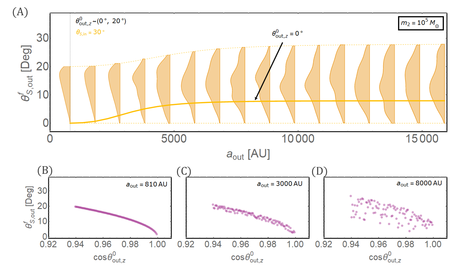
Figure 13: Panel (A) shows the PDF distribution of the angles $\theta_{\mathrm{S},\mathrm{out}}^{\mathrm{f}}$ for different $a_{\mathrm{out}}$. The parameters are the same as in Figure 12, except for each $a_{\mathrm{out}}$, we choose 100 values of $\theta_{\mathrm{out},\mathrm{z}}$ within the range of [$0^{\circ}$, $20^{\circ}$] (uniform in $\cos\theta_{\mathrm{out},\mathrm{z}}$) and the initial phase angle is set to be randomly distributed from $0$ to $2\pi$. The dashed lines are given by $\theta_{\mathrm{S},\mathrm{out}}^{\mathrm{f}}=0^{\circ}$ and $\theta_{\mathrm{S},\mathrm{out}}^{\mathrm{f}}=\theta_{\mathrm{eff},\mathrm{out}}^{0}$ with the initial $\theta_{\mathrm{out},\mathrm{z}}^{0}=20^{\circ}$ at $\varphi=\pi$. We highlight the results from $\theta_{\mathrm{out},\mathrm{z}}^{0}=0^{\circ}$ as the solid line. Panels (B)-(D) show the distribution of $\theta_{\mathrm{S},\mathrm{out}}^{\mathrm{f}}$ as a function of $\cos\theta_{\mathrm{out},\mathrm{z}}$, for three values of $a_{\mathrm{out}}$.

We now consider the general case in which $\hat{\bm{l}}$ is not aligned with $\hat{\bm{l}}_{\mathrm{in}}$ initially, focusing on systems with $m_{1}=4\times 10^{6}M_{\odot}$, $m_{2}=10^{5}M_{\odot}$.

Figure 12 shows our results when the initial $\hat{\bm{l}}$ is inclined to $\hat{\bm{l}}_{\mathrm{in}}$ by $20^{\circ}$. We find that the analytical results for $\theta_{\mathrm{S},\mathrm{out}}^{\mathrm{f}}$ agree well with the numerical results. In addition, we see that three lines from different initial phase angles converge into a single line at small $a_{\mathrm{out}}$. This is because in this case, $\bm{\Omega}_{\mathrm{eff}}\simeq-\Omega_{\mathrm{out}}^{\mathrm{(N)}}(\hat{\bm{l}}_{\mathrm{in}}\cdot\hat{\bm{l}})\hat{\bm{l}}_{\mathrm{in}}$, and $\theta_{\mathrm{S},\mathrm{out}}^{\mathrm{f}}$ is only determined by $I_{0}$ instead of $\varphi$. If $a_{\mathrm{out}}$ is sufficient large, $\bm{\Omega}_{\mathrm{eff}}\simeq-\Omega_{\mathrm{in}}\hat{\bm{J}}$ and $\theta_{\mathrm{S},\mathrm{out}}^{\mathrm{f}}=\theta_{0}$, which depends on the initial phase angle. As seem in the panel (A) of Figure 3, the minimum and maximum values of $\theta_{0}$ can be achieved when $\varphi=0^{\circ},180^{\circ}$, respectively. Therefore, the range of $\theta_{\mathrm{S},\mathrm{out}}^{\mathrm{f}}$ can be well characterized for the distant test-particle orbits.

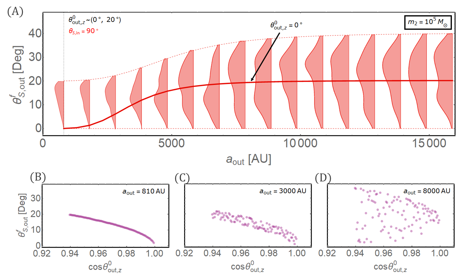
Figure 14: Same as Figure 13, except for $\theta_{\mathrm{S},\mathrm{in}}^{0}=90^{\circ}$.

To determine the final orientation of a stellar disk with finite “thickness”, we consider a range of initially inclined $\hat{\bm{l}}$ with misalignment angle $\theta_{\mathrm{out},\mathrm{z}}\in(0^{\circ},20^{\circ})$ ($\theta_{\mathrm{out},\mathrm{z}}$ is the angle between $\hat{\bm{l}}$ and $z-$axis, i.e., initial $\hat{\bm{l}}_{\mathrm{in}}$) at each $a_{\mathrm{out}}$. For each $I_{0}$, we consider a random phase $\varphi$ from $0$ to $2\pi$. The results are shown in Figure 13. A wide range of $\theta_{\mathrm{S},\mathrm{out}}^{\mathrm{f}}$ are produced for a given $a_{\mathrm{out}}$.

To characterize the role of the initial spin orientation, we perform the similar calculations with $\theta_{\mathrm{S},\mathrm{in}}^{0}=90^{\circ}$. The results are shown in Figure 14. Compared to Figure 13, the distribution of $\theta_{\mathrm{S},\mathrm{out}}^{\mathrm{f}}$ is widened, but all $\theta_{\mathrm{S},\mathrm{out}}^{\mathrm{f}}$ values are within $40^{\circ}$.

5.2 Eccentric Outer Orbits

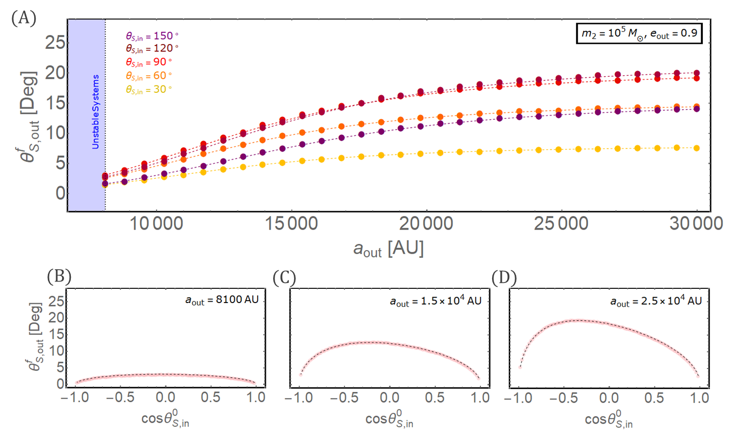
Figure 15: Same as Figure 6, except for $e=0.9$ and larger $a_{\mathrm{out}}$ due to the stability.

Here we consider how the results are changed when the outer orbits have finite eccentricities.

Figure 15 presents the results from the fiducial example (see Figure 6) but with $e=0.9$. Since the outer eccentricity $e$ only appears in the expression for $\Omega_{\mathrm{out}}^{\mathrm{(N)}}$, we carry out the analytical calculations by using Equation (11) with $e\neq 0$. We find that the numerical results and the analytical calculations are still in good agreement.

Note that here we do not consider the mutual interactions between different outer orbits. For the realistic system, the adjacent eccentric outer orbits could experience orbital crossings. But we expect the results for $\theta_{\mathrm{S},\mathrm{out}}^{\mathrm{f}}$ remain largely valid.

6 Discussion and conclusion

In this paper, we have studied the secular dynamics of stars (modeled as test particles) around a merging massive/supermassive BH binary (BHB), taking into account the GR effect induced by the rotating BH in the inner binary. We focus on the circular BHB with relatively small mass ratio, so that we only need to include the spin of the (more massive) primary BH. Our goal is to determine the final orbital orientations of the outer (circumbinary) stellar orbits relative to the spin axis of the merger remanent, assuming the initial stellar orbital axes are approximately aligned with the BHB orbital axis.

The evolution of the angular momentum vector of the stellar orbit ($\hat{\bm{l}}$) is determined by the competition between the precession of the BHB axis $\hat{\bm{l}}_{\mathrm{in}}$ around the primary spin axis $\hat{\bm{S}}_{1}$ and the precession of $\hat{\bm{l}}$ around $\hat{\bm{l}}_{\mathrm{in}}$. During the orbital decay of the BHB, the ratio of the two precession rates can change from $\lesssim 1$ to $\gtrsim 1$, leading to a significant change in the orientation of $\hat{\bm{l}}$. The final direction of $\hat{\bm{l}}$ carries the imprint of the spin of the remanent BH ($\hat{\bm{S}}_{1}$). Our main findings are:

(i) For central BHBs with modest mass ratio ($m_{2}/m_{1}\sim 0.1$), there is a quasi-alignment phenomenon for the evolution of the outer stellar orbits. Namely, starting with nearly coplanar outer orbits (i.e., $\hat{\bm{l}}\parallel\hat{\bm{l}}_{\mathrm{in}}$), the orbital axis $\hat{\bm{l}}$ of the circumbinary star will preferentially evolve towards the spin direction after the merger of inner BHB, regardless the initial spin-orbit misalignment angle of the BHB (see Figure 6). This alignment is particularly strong for close stellar orbits. Such trend of alignment, where the final spin-orbit misalignment angle ($\theta_{\mathrm{S},\mathrm{out}}^{\mathrm{f}}$) is small, can be understood analytically based on the principle of adiabatic invariance (Equation 35). Also, our analytical analysis can be applied to inclined and eccentric outer orbits (Figures 13, 14 and 15).

(ii) When the mass ratio of the BHB is more extreme (i.e., $m_{2}/m_{1}\lesssim 0.01$), the angular momentum axis of the outer stellar orbit can experience complicated evolution in general. The adiabaticity condition in the analytical calculation may break down and the evolution of the stellar orbits can only be resolved numerically by using the full secular equations of motion. Nevertheless, the alignment effect still works reasonably well when the initial spin-orbit misalignment angle is small (i.e., $\theta_{\mathrm{S},\mathrm{in}}^{0}\lesssim 90^{\circ}$; see Figures 8 and 10).

There are several caveats in our study:

(i) We have neglected the effect due to the secondary spin in the central BHB. This is reasonable if the secondary spin $S_{2}$ is negligible compared to $S_{1}$ (e.g., when the mass ratio $m_{2}/m_{1}$ is relatively small or when $\chi_{2}\ll\chi_{1}$). For comparable-mass BHBs, the final spin axis the merger remnant is approximately aligned with the pre-merger orbital axis, thus we expect the circumbinary stellar orbital axis to be aligned with the final BH spin (assuming $\hat{\bm{l}}$ is initially aligned with the binary axis).

(ii) We have not considered the merger kick acting on the remnant BH, which may change the orientation of the stellar orbit relative to the final BH spin axis. For the BHB studied in our paper ($m_{1}=4\times 10^{6}M_{\odot}$ and $m_{2}=10^{5}M_{\odot}$, with mass ratio $0.025$), assuming the primary BH has the maximum spin with isotropic orientation, the kick velocity ($V_{\mathrm{kick}}$) on the merger remnant evaluated using the fitting formula of Lousto et al. (2010) is less than $\sim 40\mathrm{km/s}$. Compared to the orbital velocity ($V_{\mathrm{orb}}$) of the stellar orbits studied here ($a_{\mathrm{out}}\lesssim 10^{5}$AU), we always have $V_{\mathrm{orb}}\gg V_{\mathrm{kick}}$. Thus, the kick effect is negligible. However, for BHBs with higher mass ratios, the merger kick could play an important role, especially for the distant stellar orbits with $V_{\mathrm{orb}}\gtrsim V_{\mathrm{kick}}$. In this case, the post-kick orbital orientation can be modified (e.g., Liu & Lai, 2021), and the final spin-orbit misalignment angle must be evaluated based on the corrected orientation of $\hat{\bm{l}}$.

(iii) We have only considered BHBs in circular orbit in this paper. When the BHB has a finite eccentricity, the outer stellar orbit can also gain modest eccentricity through octupole-order secular interactions (e.g., Liu et al., 2015a, b). The finite eccentricity may influence the orbital inclination evolution indirectly.

Our result suggests that the relative orientation between the spin of a central massive/supermassive BH and the surrounding stellar orbits might provide a probe of the merger history of the BH. In particular, the Galactic Center hosts a population of young massive stars (e.g., Ghez et al., 1998, 2008; Genzel et al., 2000; Merritt, 2013; Alexander, 2017). If the supermassive BH, Sagittarius A^∗, has experienced a previous merger with an intermediate-mass BH, it could have left some imprints on the nearby S-star orbits. It has been suggested that the orbital distribution of S-stars could put constraints on the Sagittarius A^∗ spin (e.g., Levin & Beloborodov, 2003; Fragione & Loeb, 2020). Therefore, the precise measurements of the S-star orbits (including the orbital orientations) and the spin axis of central BH would be highly desirable.

7 Acknowledgments

BL thanks Johan Samsing, Daniel D’Orazio and Adrian Hamers for useful discussion. DL has been supported in part by NSF grants AST-1715246 and AST-2107796. This project has received funding from the European Union’s Horizon 2020 research and innovation program under the Marie Sklodowska-Curie grant agreement No. 847523 ‘INTERACTIONS’.

8 DATA AVAILABILITY

The simulation data underlying this article will be shared on reasonable request to the corresponding author.

References

- Alexander (2017) Alexander T., 2017, ARA&A, 55, 17
- Bansal et al. (2017) Bansal K., Taylor G. B., Peck A. B., Zavala R. T., Romani R. W., 2017, ApJ, 843, 14
- Barker & O’Connell (1975) Barker B. M., O’Connell R. F., 1975, PhRvD, 12, 329
- Begelman et al. (1980) Begelman M. C., Blandford R. D., Rees M. J., 1980, Nature, 287, 307
- Bianchi et al. (2008) Bianchi S., Chiaberge M., Piconcelli E., Guainazzi M., Matt G., 2008, MNRAS, 386, 105
- Bogdanović et al. (2009) Bogdanović T., Eracleous M., Sigurdsson S., 2009, ApJ, 697, 288
- Boroson & Lauer (2009) Boroson T. A., Lauer T. R., 2009, Nature, 458, 53
- Chapon et al. (2013) Chapon D., Mayer L., Teyssier R., 2013, MNRAS, 429, 3114
- Comerford et al. (2009) Comerford J. M., Griffith R. L., Gerke B. F., Cooper M. C., Newman J. A., Davis M., Stern D., 2009, ApJL, 702, L82
- Comerford et al. (2018) Comerford J. M., Nevin R., Stemo A., Müller-Sánchez F., Barrows R. S., Cooper M. C., Newman J. A., 2018, ApJ, 867, 66
- Cuadra et al. (2009) Cuadra J., Armitage P. J., Alexander R. D., Begelman M. C., 2009, MNRAS, 393, 1423
- Deane et al. (2014) Deane R. P., Paragi Z., Jarvis M. J., Coriat M., Bernardi G., Fender R. P., Frey S., et al., 2014, Nature, 511, 57
- De Rosa et al. (2019) De Rosa A., Vignali C., Bogdanović T., Capelo P. R., Charisi M., Dotti M., Husemann B., et al., 2019, NewAR, 86, 101525
- Dotti et al. (2007) Dotti M., Colpi M., Haardt F., Mayer L., 2007, MNRAS, 379, 956
- Dotti et al. (2009) Dotti M., Montuori C., Decarli R., Volonteri M., Colpi M., Haardt F., 2009, MNRAS, 398, L73
- Escala et al. (2005) Escala A., Larson R. B., Coppi P. S., Mardones D., 2005, ApJ, 630, 152
- Farago & Laskar (2010) Farago F., Laskar J., 2010, MNRAS, 401, 1189
- Ford et al. (2000) Ford E. B., Kozinsky B., Rasio F. A., 2000b, ApJ, 535, 385
- Fragione & Loeb (2020) Fragione, G. & Loeb, A. 2020, ApJL, 901, L32
- Fragione (2022) Fragione G., 2022, arXiv, arXiv:2202.05618
- Gallardo et al. (2012) Gallardo T., Hugo G., Pais P., 2012, Icar, 220, 392
- Genzel et al. (2000) Genzel R., Pichon C., Eckart A., Gerhard O. E., Ott T., 2000, MNRAS, 317, 348
- Ghez et al. (1998) Ghez A. M., Klein B. L., Morris M., Becklin E. E., 1998, ApJ, 509, 678
- Ghez et al. (2008) Ghez A. M., Salim S., Weinberg N. N., Lu J. R., Do T., Dunn J. K., Matthews K., et al., 2008, ApJ, 689, 1044
- Green et al. (2010) Green P. J., Myers A. D., Barkhouse W. A., Mulchaey J. S., Bennert V. N., Cox T. J., Aldcroft T. L., 2010, ApJ, 710, 1578
- Holman & Wiegert (1999) Holman M. J., Wiegert P. A., 1999, AJ, 117, 621
- Komossa et al. (2003) Komossa S., Burwitz V., Hasinger G., Predehl P., Kaastra J. S., Ikebe Y., 2003, ApJL, 582, L15
- Komossa et al. (2008) Komossa S., Zhou H., Lu H., 2008, ApJL, 678, L81
- Kozai (1962) Kozai Y., 1962, AJ, 67, 591
- Levin & Beloborodov (2003) Levin Y., Beloborodov A. M., 2003, ApJL, 590, L33
- Li et al. (2014) Li D., Zhou J.-L., Zhang H., 2014, MNRAS, 437, 3832
- Lidov (1962) Lidov M. L., 1962, Planet. Space Sci., 9, 719
- Liu et al. (2015a) Liu B., Muñoz D. J., Lai D., 2015a, MNRAS, 447, 747
- Liu et al. (2015b) Liu B., Lai D., Yuan Y.-F., 2015b, PhRvD, 92, 124048
- Liu et al. (2019) Liu B., Lai D., Wang Y.-H., 2019, ApJL, 883, L7
- Liu & Lai (2020) Liu B., Lai D., 2020, PhRvD, 102, 023020
- Liu & Lai (2021) Liu B., Lai D., 2021, MNRAS, 502, 2049
- Liu & Lai (2022) Liu B., Lai D., 2022, ApJ, 924, 127.
- Liu et al. (2014) Liu X., Shen Y., Bian F., Loeb A., Tremaine S., 2014, ApJ, 789, 140
- Lousto et al. (2010) Lousto C. O., Campanelli M., Zlochower Y., Nakano H., 2010, CQGra, 27, 114006
- Mayer et al. (2007) Mayer L., Kazantzidis S., Madau P., Colpi M., Quinn T., Wadsley J., 2007, Sci, 316, 1874
- Merritt (2013) Merritt D., 2013, degn.book
- Milosavljević & Merritt (2001) Milosavljević M., Merritt D., 2001, ApJ, 563, 34
- Milosavljević & Phinney (2005) Milosavljević M., Phinney E. S., 2005, ApJL, 622, L93
- Naoz (2016) Naoz S., 2016, ARA&A, 54, 441
- Naoz et al. (2017) Naoz S., Li G., Zanardi M., de Elía G. C., Di Sisto R. P., 2017, AJ, 154, 18
- Peters (1964) Peters P. C., 1964, PhRv, 136, 1224
- Petrovich (2015) Petrovich C., 2015, ApJ, 799, 27
- Rodriguez et al. (2006) Rodriguez C., Taylor G. B., Zavala R. T., Peck A. B., Pollack L. K., Romani R. W., 2006, ApJ, 646, 49
- Sillanpaa et al. (1988) Sillanpaa A., Haarala S., Valtonen M. J., Sundelius B., Byrd G. G., 1988, ApJ, 325, 628
- Tagawa et al. (2020) Tagawa H., Haiman Z., Kocsis B., 2020, ApJ, 898, 25
- Tagawa et al. (2021) Tagawa H., Kocsis B., Haiman Z., Bartos I., Omukai K., Samsing J., 2021, ApJ, 908, 194
- Vinson & Chiang (2018) Vinson B. R., Chiang E., 2018, MNRAS, 474, 4855
- von Zeipel (1910) von Zeipel H., 1910, AN, 183, 345
- Zanazzi & Lai (2018) Zanazzi J. J., Lai D., 2018, MNRAS, 473, 603