Steerable Pyramid Transform Enables
Robust Left Ventricle Quantification

Abstract

Although multifarious variants of convolutional neural networks (CNNs) have proved successful in cardiac index quantification, they seem vulnerable to mild input perturbations, e.g., spatial transformations, image distortions, and adversarial attacks. Such brittleness erodes our trust in CNN-based automated diagnosis of various cardiovascular diseases. In this work, we describe a simple and effective method to learn robust CNNs for left ventricle (LV) quantification, including cavity and myocardium areas, directional dimensions, and regional wall thicknesses. The key to the success of our approach is the use of the biologically-inspired steerable pyramid transform (SPT) as fixed front-end processing, which brings three computational advantages to LV quantification. First, the basis functions of SPT match the anatomical structure of the LV as well as the geometric characteristics of the estimated indices. Second, SPT enables sharing a CNN across different orientations as a form of parameter regularization, and explicitly captures the scale variations of the LV in a natural way. Third, the residual highpass subband can be conveniently discarded to further encourage robust feature learning. A concise and effective metric, named Robustness Ratio, is proposed to evaluate the robustness under various input perturbations. Extensive experiments on $145$ cardiac sequences show that our SPT-augmented method performs favorably against state-of-the-art algorithms in terms of prediction accuracy, but is significantly more robust under input perturbations.

Left ventricle quantification, steerable pyramid transform, model robustness.

1 Introduction

Cardiovascular diseases cause so far the largest mortality among all pathologies worldwide, with millions of premature deaths every year [1]. Therefore, quantifying structural and physiological cardiac indices, especially those relevant to the left ventricle (LV) due to its central role in powering the systemic circulation, has attracted extensive academic and clinical attention [2].

Among various imaging techniques, the non-invasive cardiovascular magnetic resonance (CMR) has become a gold standard to acquire the anatomical and functional information of the heart, generating image sequences in decent resolution and good contrast between soft tissues [3, 4]. Moreover, CMR comes with different imaging protocols [2], such as cine CMR to provide high spatiotemporal resolution with high contrast, flow CMR to encode the velocity information of the cardiovascular flow, tagged CMR to assess regional dysfunction, etc. CMR-based LV quantification aims to provide a comprehensive, objective, and accurate evaluation of the LV pathological changes through structural index prediction. A commonly used setting for LV quantification is to take a sequence of CMR slices (i.e., images) within one cardiac cycle as input, and produce a set of structural indices for each slice, e.g., cavity and myocardium areas, three directional dimensions, and six regional wall thicknesses [5, 6], as shown in Fig. 1. Important functional indices (e.g., LV stroke volume and ejection fraction) can then be inferred subsequently.

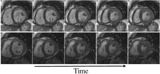
(a)

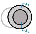
(b)

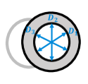
(c)

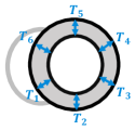
(d)

Figure 1: A popular setting in LV quantification. (a) Two representative sequences of CMR slices with different shapes, brightness, and contrast. (b) LV myocardium area ($A_{1}$) and cavity area ($A_{2}$). (c) Three directional dimensions of the cavity ($D_{1}\sim D_{3}$). (d) Six regional wall thicknesses ($T_{1}\sim T_{6}$).

Existing LV quantification approaches focus primarily on improving the accuracy, e.g., in terms of mean absolute error between model predictions and human annotations. This leads to an impressive series of sophisticated methods from indirect segmentation and direct regression to multi-task relationship learning [6], and from CMR statistics-based to deep learning-based methods. Despite the demonstrated success, few investigations have been made into testing and improving the robustness of LV quantification. Not surprisingly, mild input perturbations that may occur in the lifetime of CMR images (from acquisition, storage, transmission, and clinical applications) suffice to falsify nearly all existing LV quantification methods. Such brittleness hinders the practical early diagnosis and risk stratification of multifarious cardiovascular diseases, and may even arouse widespread public concerns and anxieties about insurance fraud via medical report manipulation [7].

Rather than chasing the state-of-the-art LV quantification performance on standard benchmarks, we switch our attention to testing and improving the robustness of LV quantification based on convolutional neural networks (CNNs). The crux of our approach is to incorporate the steerable pyramid transform (SPT) [8] as a fixed biologically-inspired front-end, which captures invariant (or equivariant) features considered elemental for visual information processing (e.g., local orientation and scale). Despite its simplicity, SPT brings three computational advantages to CNN-based LV quantification. First, the convolutional basis filters of SPT are localized in orientation and scale, whose responses are translation-equivariant (i.e., aliasing-free) and rotation-equivariant (i.e., steerable). This nice property matches the anatomical structures and spatiotemporal dynamics of the LV, as well as the geometric characteristics of the estimated indices. Second, SPT offers a straightforward implementation of parameter sharing across orientations as a form of regularization, and models the scale variation of the LV during one cardiac cycle and among different subjects in an explicit way. Third, the residual highpass subband as one source of model vulnerability [9] can be conveniently discarded to encourage more robust cardiac representation learning. Extensive experiments demonstrate that our SPT-augmented method predicts the eleven LV indices accurately, and is significantly more robust compared to existing methods under spatial transformations, common image distortions, and adversarial attacks.

The remainder of this paper is organized as follows. Section 2 discusses the related work and reviews SPT used in this work. Section 3 presents in detail the proposed method for robust LV quantification. The main experimental results are given in Section 4, followed by comprehensive ablation studies to justify the effectiveness of design choices of the proposed method. We conclude and discuss in Section 5.

2 Related Work

In this section, we first summarize previous work on LV quantification. We then review SPT and its applications, especially in the era of deep learning.

2.1 LV Quantification

Early LV qualification relied exclusively on the manual delineation of cardiac boundaries, which is a tedious, time-consuming yet professional task. Thus it is highly desirable to construct computational methods that automate the quantification process to facilitate the pre-screening and diagnosis of cardiovascular diseases. The majority of previous work focused on semi-automatic or fully automatic segmentation of LV contours [2], which were thought to be necessary for predicting various structural and functional LV indices. Image-based segmentation methods leverage ideas from the field of signal and image processing, with representative techniques including thresholding, region growing, pixel/voxel-level classification, and active contour [2]. Model-based methods make use of strong shape priors in the form of cardiac atlases to improve the segmentation results [10, 11]. Recently, CNN-based segmentation methods have also begun to emerge [12], built on top of well-known network architectures like FCN [13], U-Net [14], and 3D-CNN [15]. Despite being fairly interpretable, segmentation-based methods require pixel-level dense prediction, which is a more difficult problem formulation compared to image-level global prediction. Moreover, a recent study [16] showed that it is trivial to expose semantic segmentation failures of natural images via a computational procedure called maximum discrepancy competition [17]. It is thus reasonable to cast doubts on the robustness of cardiac image segmentation as similar techniques have been applied.

Direct regression methods seek to fit mapping functions between CMR images and the associated indices without explicit delineation of cardiac boundaries. Along this line, many CMR statistics have been handcrafted, including pyramidal Gabor features, histogram of oriented gradients [18], blob-like features [19], blood homogeneity, and segment distribution similarity. Zhen et al. [20] adopted a convolutional variant of restricted Boltzmann machine to learn cardiac representation from unlabeled CMR images. They sought for a compact and low-rank representation by minimizing the reconstruction loss with smooth manifold regularization. With the availability of large human-labeled CMR image datasets [21, 22], the problem of LV quantification has been revolutionized by CNNs [5, 6, 23, 24]. Of particular interest is the deep multi-task relationship learning work by Xue et al.[6], which effectively models the correlations among different indices, and offers state-of-the-art quantification performance. Although these methods have achieved high accuracy numbers, they are quite vulnerable to mild and even imperceptible input perturbations, which may come along with the CMR images during acquisition, storage, transmission, processing, and clinical applications. Unlike previous efforts, we aim for a robust and accurate LV quantification method in this work.

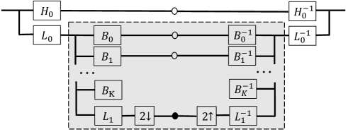
Figure 2: The block diagram for SPT (both analysis and synthesis), reproduced from [8]. The recursive construction of a pyramid is achieved by inserting a copy of the shaded portion of the diagram at the location of the solid circle [8].

2.2 Steerable Pyramid Transform (SPT)

As a linear multi-scale multi-orientation image decomposition, SPT was developed by Simoncelli et al. [8, 25] in the 1990s to overcome the limitations of orthogonal wavelets. The basis functions are the $K$-th order directional derivative filters, which have different sizes and $K+1$ orientations. As shown in Fig. 2, SPT first decomposes an image $\bm{x}$ into high and lowpass subbands using filters $H_{0}$ and $L_{0}$. The lowpass subband is then separated into a set of oriented subbands by a bank of filters $\{B_{k}\}_{k=0}^{K}$ and a lower-pass subband by the filter $L_{1}$ with a stride of two (i.e., down-sampled by a factor of two along both spatial dimensions). This lower-pass subband can be recursively decomposed to obtain the steerable pyramid. An example decomposition of a CMR image, containing three orientations at two scales, is shown in Fig. 3.

Over the past three decades, SPT has been demonstrated useful in a variety of image processing and computer vision applications, ranging from low-level tasks - image denoising [26], image compression [27], image steganalysis [28], and image quality assessment [29], middle-level tasks - texture synthesis [30] and image segmentation [31], to high-level tasks - object detection and visual tracking [32]. In the era of deep learning, Meyer et al. [33] proposed PhaseNet for video frame interpolation. They trained a CNN to estimate the SPT phase decomposition of the intermediate frame. Bhardwaj et al. [34] proposed an unsupervised information-theoretic perceptual quality metric using SPT as the fixed input transformation. Deng et al. [35] adopted inter-frame phase differences by SPT rather than optical flow to enhance video emotion recognition. Parthasarathy and Simoncelli developed a two-stage visual texture model using SPT and a learnable bank of convolution filters to mimic the V1 simple and V2 complex cells, respectively [36]. Most existing work incorporates SPT to improve the accuracy of computational predictions. In contrast, we probe the added robustness of SPT to CNN-based LV quantification.

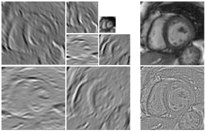
Figure 3: Visual illustration of SPT of a CMR image, containing three orientations at two scales. Left panel: Subbands oriented at $30\degree$, $90\degree$, and $150\degree$, respectively. The smallest subband contains the residual lowpass information. Right panel: Original CMR image and its residual highpass subband.

3 Proposed Method

In this section, we describe our SPT-augmented CNN-based method for robust and accurate LV quantification. At a high level, we decompose each slice in a CMR image sequence into a steerable pyramid with three orientations at two scales. We then use a five-layer CNN to map the pyramid representation of each slice to three oriented feature vectors, which are fed to a shared long short-term memory (LSTM) [37] to predict the eleven structural LV indices. The learning of the entire method is driven by the mean absolute error (MAE) and a regularizer of the multi-task relationships. The system diagram is shown in Fig. 4.

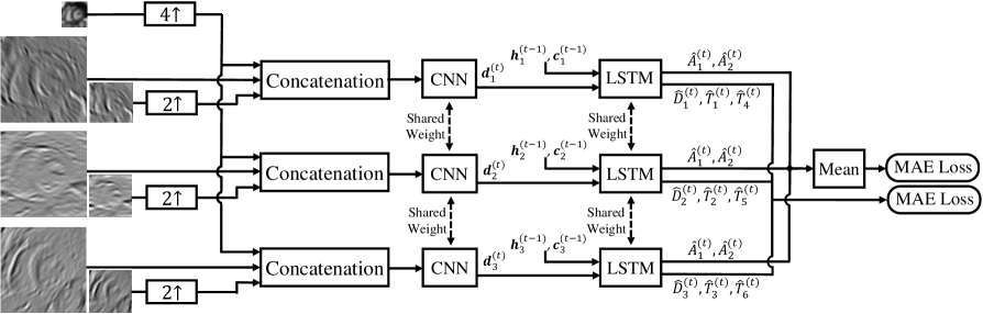
Figure 4: The system diagram of the proposed SPT-augmented method for robust LV quantification.

3.1 SPT Decomposition

Given an input slice $\bm{x}\in\mathbb{R}^{M\times N}$, we decompose it into a steerable pyramid $\{\bm{x}_{i}\}_{i=0}^{7}$, where $\bm{x}_{0}\in\mathbb{R}^{\left\lfloor\frac{M}{4}\right\rfloor\times\left\lfloor\frac{N}{4}\right\rfloor}$ and $\bm{x}_{7}\in\mathbb{R}^{M\times N}$ are residual lowpass and highpass subbands, respectively. $\bm{x}_{1},\bm{x}_{2},\bm{x}_{3}\in\mathbb{R}^{\left\lfloor\frac{M}{2}\right\rfloor\times\left\lfloor\frac{N}{2}\right\rfloor}$ are three oriented subbands to $30\degree$, $90\degree$, and $150\degree$, respectively, at Scale 2. Similarly, $\bm{x}_{4},\bm{x}_{5},\bm{x}_{6}\in\mathbb{R}^{M\times N}$ are three oriented subbands at Scale 1 (i.e., the same scale as the original slice). We set the number of scales to two because the LV slice $\bm{x}$ is often a small region of interest within the cardiac image, which is of limited resolution (e.g., $80\times 80$). We use three orientations at $\{30\degree,90\degree,150\degree\}$ because the mid-cavity myocardium is an approximate 2D torus in the short-axis view, and both directional dimensions and regional wall thicknesses are distributed at the same orientations, which can be seen in Fig. 5.

After specifying the hyperparameter setting of the steerable pyramid, it remains to determine how to organize the pyramid as the input to the CNN. Towards this, we make two key observations. First, from the computational neuroscience literature [38, 39], we learn that humans rely primarily on low-frequency information to perform object recognition. However, CNNs tend to exploit high-frequency information that is imperceptible to the human eye [9, 40], leading to peculiar generalization behaviors that perceptually deviate from humans, including adversarial vulnerability. Thus, we choose to discard the highpass subband $\bm{x}_{7}$, forcing the CNN to learn robust cardiac representation from lowpass and oriented subbands. Second, SPT allows independent representation of orientation and scale [8]. In the context of LV quantification, orientation is more relevant to spatial predictions of LV indices, such as the three directional dimensions and six regional wall thicknesses. Scale, on the other hand, is more relevant to temporal predictions of these indices, which vary with the myocardial contraction and relaxation. To learn robust spatiotemporal cardiac representation, we choose to gather all scale subbands of the same orientation together with the lowpass subband as the input of the CNN to predict the five corresponding indices. For example, we use $\{\bm{x}_{0},\bm{x}_{1},\bm{x}_{4}\}$ to predict $\{A_{1},A_{2},D_{1},T_{1},T_{4}\}$ (see the correspondence in Fig. 1). The parameters of the CNN-based method are shared across different orientations. Such data organization can be viewed as a way of parameter regularization, encouraging the CNN to attend to different directional visual cues. Moreover, we explicitly model the scale variation of the LV from diastole to systole and across different subjects since the input subbands (e.g., $\{\bm{x}_{0},\bm{x}_{1},\bm{x}_{4}\}$) live in three different scales. There is an efficient implementation of the proposed data organization by allocating orientation and scale/lowpass subbands in the batch and channel dimensions, respectively. Bilinear interpolation is used to resample small-scale subbands to the size of the original image.

3.2 LV Quantification

After SPT, a generic five-layer CNN is constructed to extract spatially oriented features. Within the CNN, each layer applies a bank of convolution filters, whose responses are batch-normalized and half-wave rectified (i.e., ReLU). A max-pooling operation is added to the first four convolution layers to down-sample the rectified responses by a factor of two along both spatial dimensions. We compensate for spatial down-sampling by doubling the number of filters (i.e., channels). We use global $L_{2}$-pooling to summarize the remaining spatial information into a fixed-length feature vector, which is further processed by a fully connected layer with dropout regularization. The detailed specification is shown in Fig. 6. After the CNN, we represent the LV slice $\bm{x}$ by $\{\bm{d}_{i}\}_{i=1}^{3}$, where $\bm{d}_{i}\in\mathbb{R}^{C\times 1}$ is the $i$-th orientation feature vector.

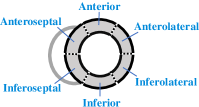
(a)

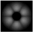
(b)

Figure 5: Regional walls of the mid-cavity LV myocardium by the $17$-segment model [41] and the corresponding frequency bands of SPT in Fourier domain.

Figure 6: The architecture of the CNN for spatial feature extraction. The parameterization of the convolution and pooling layers is denoted as “kernel size $\mid$ input channel $\times$ output channel $\mid$ stride” and “kernel size $\mid$ stride”, respectively. The number of parameters for each layer is given at the bottom, yielding a total of $4.07$ million.

Next, we adopt an LSTM following the CNN to model the temporal dynamics of the LV during the myocardial contraction and relaxation, respectively. The LSTM cell relies on the hidden state vector (also known as the output vector of the LSTM) of the previous LV slice, $\bm{h}^{(t-1)}\in\mathbb{R}^{C\times 1}$ and the feature vector of the current slice, $\bm{d}^{(t)}$ to compute three gates and one intermediate cell state vector:

$$\bm{f}^{(t)} =\mathrm{sigmoid}\left(\bm{W}_{f}[\bm{d}^{(t)};\bm{h}^{(t-1)}]+\bm{b}_{f}\right),$$ (1)

$$\bm{i}^{(t)} =\mathrm{sigmoid}\left(\bm{W}_{\mathrm{in}}[\bm{d}^{(t)};\bm{h}^{(t-1)}]+\bm{b}_{\mathrm{in}}\right),$$ (2)

$$\bm{o}^{(t)} =\mathrm{sigmoid}\left(\bm{W}_{\mathrm{out}}[\bm{d}^{(t)};\bm{h}^{(t-1)}]+\bm{b}_{\mathrm{out}}\right),$$ (3)

$$\tilde{\bm{c}}^{(t)} =\mathrm{tanh}\left(\bm{W}_{c}[\bm{d}^{(t)};\bm{h}^{(t-1)}]+\bm{b}_{c}\right),$$ (4)

where $\bm{W}_{f},\bm{W}_{\mathrm{in}},\bm{W}_{\mathrm{out}},\bm{W}_{c}\in\mathbb{R}^{C\times 2C}$ and $\bm{b}_{f},\bm{b}_{\mathrm{in}},\bm{b}_{\mathrm{out}},\bm{b}_{c}\in\mathbb{R}^{C\times 1}$ are the weight matrices and the bias vectors, respectively. $\bm{f}^{(t)}$, $\bm{i}^{(t)}$, and $\tilde{\bm{c}}^{(t)}$ together are used to update the cell state vector:

$$\bm{c}^{(t)}=\bm{f}^{(t)}\odot\bm{c}^{(t-1)}+\bm{i}^{(t)}\odot\tilde{\bm{c}}^{(t)},$$ (5)

where $\odot$ denotes the element-wise product. Last, the current hidden state vector is computed by

$$\bm{h}^{(t)}=\bm{o}^{(t)}\odot\mathrm{tanh}(\bm{c}^{(t)}).$$ (6)

It is worth noting that in Eqs. (1) to (6), we omit the subscript index $i$ because the LSTM cell is shared across orientations. After the LSTM, we represent the $t$-th LV slice $\bm{x}^{(t)}$ by $\{\bm{h}^{(t)}_{i}\}_{i=1}^{3}$, based on which we use linear regression to predict the eleven LV indices:

$$[\hat{A}^{(t)}_{1,i};\hat{A}^{(t)}_{2,i};\hat{D}^{(t)}_{i};\hat{T}^{(t)}_{i};\hat{T}^{(t)}_{i+3}]=\bm{W}_{i}\bm{h}_{i}^{(t)}+\bm{b}_{i},i=1,2,3,$$ (7)

where $\bm{W}_{i}\in\mathbb{R}^{5\times C}$ and $\bm{b}_{i}\in\mathbb{R}^{5\times 1}$ are the $i$-th weight matrix and bias term to be optimized. In other words, the $i$-th orientation feature is responsible for estimating two cavity areas $\hat{A}^{(t)}_{1,i}$ and $\hat{A}^{(t)}_{2,i}$, one corresponding directional dimension $\hat{D}_{i}^{(t)}$, and two corresponding wall thicknesses $\hat{T}_{i}^{(t)}$ and $\hat{T}_{i+3}^{(t)}$. The final cavity and myocardium areas are computed by averaging predictions from the three orientation predictions:

$$\hat{A}^{(t)}_{r}=\frac{1}{3}\sum_{i=1}^{3}\hat{A}^{(t)}_{r,i},\quad r=1,2.$$ (8)

3.3 Loss Function

For notation convenience, we collectively denote all eleven predictions of the LV indices by $\hat{\bm{y}}=\bm{g}_{\bm{\theta}}(\bm{x})\in\mathbb{R}^{11\times 1}$, where $\bm{g}$ denotes the entire LV quantification method, parameterized by $\bm{\theta}$. We adopt the MAE as the loss function:

$$\ell_{1}(\bm{\theta};\mathcal{B})=\frac{1}{|\mathcal{B}|}\sum_{(\bm{x},\bm{y})\in\mathcal{B}}\|\bm{y}-\bm{g}_{\bm{\theta}}({\bm{x}})\|_{1},$$ (9)

where $\mathcal{B}$ is a mini-batch of training examples sampled from the full dataset. To enable a fair comparison with [6], we also enforce three levels of correlation constraints on the parameters of the final linear regression $\bm{W}_{\mathrm{lr}}\coloneqq\{\bm{W}_{1},\bm{W}_{2},\bm{W}_{3}\}\in\mathbb{R}^{D_{o}\times D_{i}\times D_{c}}$, where $D_{o}=3$, $D_{i}=5$, and $D_{c}=100$. These include orientation, index, and weight correlations, which can be summarized using a tensor Normal distribution [42] as a prior:

$$p\left(\bm{W}_{\mathrm{lr}}\right)= \mathcal{TN}\left(\bm{W}_{\mathrm{lr}};\bm{0},\bm{\Sigma}_{o},\bm{\Sigma}_{i},\bm{\Sigma}_{c}\right)$$

$$= \mathcal{N}\left(\mathrm{vec}(\bm{W}_{\mathrm{lr}});\bm{0},\bm{\Sigma}_{\mathrm{lr}}\right)$$

$$= {\left({2\pi}\right)^{-D_{o}D_{i}D_{c}/2}}{\prod_{k\in\{o,i,c\}}{{{\left|{{\bm{\Sigma}_{k}}}\right|}^{-D_{o}D_{i}D_{c}/\left({2{D_{k}}}\right)}}}}$$

$$\times\exp\left({-\frac{1}{2}{{{{\mathrm{vec}}\left(\bm{W}_{\mathrm{lr}}\right)}}^{\mathsf{T}}}\bm{\Sigma}_{\mathrm{lr}}^{-1}{\mathrm{vec}}\left(\bm{W}_{\mathrm{lr}}\right)}\right).$$ (10)

$\mathrm{vec}(\cdot)$ is the vectorized operation and ${\bm{\Sigma}_{\mathrm{lr}}}={\bm{\Sigma}_{o}}\otimes{\bm{\Sigma}_{i}}\otimes{\bm{\Sigma}_{c}}$ denotes the Kronecker product of the orientation covariance matrix ${\bm{\Sigma}_{o}}\in\mathbb{R}^{D_{o}\times D_{o}}$, the index covariance matrix ${\bm{\Sigma}_{i}}\in\mathbb{R}^{D_{i}\times D_{i}}$, and the weight covariance matrix ${\bm{\Sigma}_{c}}\in\mathbb{R}^{D_{c}\times D_{c}}$. We further assume that $\bm{y}_{i}$ is Laplace distributed with the location parameter estimated by $\hat{\bm{y}}_{i}$ and the scale parameter fixed to one. As a result, maximizing the posterior distribution of $\bm{\theta}$ is equivalent to minimizing

$$\ell(\bm{\theta},{\bm{\Sigma}}_{\mathrm{lr}};\mathcal{B})= \ell_{1}(\bm{\theta};\mathcal{B})+\lambda\Big{(}\mathrm{vec}(\bm{W}_{\mathrm{lr}})^{\mathsf{T}}\bm{\Sigma}_{\mathrm{lr}}^{-1}\mathrm{vec}(\bm{W}_{\mathrm{lr}})\Big{.}$$

$$\Big{.}-\sum_{k\in\{o,i,c\}}\frac{D_{o}D_{i}D_{c}}{D_{k}}\ln|{{\bm{\Sigma}}_{k}}|\Big{)},$$ (11)

where we assume the remaining parameters $\bm{\theta}\setminus\bm{W}_{\mathrm{lr}}$ are uniformly distributed (i.e., the possible values are equally likely). The added regularization in Eq. (3.3) has two effects. The first component in the parentheses minimizes the mode of the weights $\bm{W}_{\mathrm{lr}}$, which acts similarly as an $L_{2}$ regularization. The second component maximizes the determinant of $\bm{\Sigma}_{k}$, which encourages independent feature learning.

3.4 Robustness Evaluation

Probing the robustness of LV quantification is our primary concern. To this end, we propose a comprehensive evaluation framework. We first introduce three types of input perturbations: spatial transformations, image distortions, and adversarial attacks. Then a concise and effective evaluation criterion is proposed to describe the robustness.

Input Perturbations. Three types of input perturbations, spatial transformations, image distortions, and adversarial attacks, are considered.

The invariance of computational methods to spatial transformations has always been a research hotspot. It is a fact that most popular CNN-based models are vulnerable to even mild spatial transformations [43]. Although the data augmentation trick can be performed to gain robustness to spatial transformations, it only achieves marginal improvements and generalizes poorly to unseen transformations. Here we include 1) translation and 2) rotation. Specifically, different perturbation intensity levels are set. The maximum horizontal and/or vertical translation is set to $10\%$ of the image resolution. Each pixel of translation corresponds to one perturbation level, and there are a total of $8$ levels, where we consider the same pixels of horizontal and vertical translations as the same level. The range of rotation is set to $\left[-30\degree,30\degree\right]$ according to the position and orientation of the six myocardium regions. Every $3^{\degree}$ of rotation corresponds to one level, and there are a total of $10$ levels. We intentionally opt not to cover more complex non-linear spatial transformations as they may not be label-preserving.

For image distortions, we consider 1) additive white Gaussian noise, 2) impulsive noise, 3) Rician noise, 4) Gaussian blur, and 5) JPEG compression. Gaussian noise and blur are the most extensively examined distortions for digital signals, including medical images. Impulsive noise is commonly used to simulate the switching artifact which emerges at some time slots in adverse working environments and equipment conditions [44]. Generally, CMR image acquisition is through a single-channel radiofrequency coil and performing Fourier transform for subsequent magnitude calculations. This results in spatially homogeneously distributed image noise with Rician statistics [45, 46]. JPEG compression is ubiquitous before storing CMR images. We generate the five distortions using the same implementations to create ImageNet-C [47]. We set five intensity levels for each distortion, which are shown in Fig. 7 (d)-(h).

Adversarial attacks refer to computational methods of generating visual stimuli that often look identical to the reference examples but are catastrophic failures of the CNN being examined [48, 49]. Existing adversarial attacks are mainly crafted via gradient-based optimization [48, 49]. A perceptual constraint is enforced to ensure that the generated examples are visually similar to the unperturbed ones. A variety of defense approaches were proposed to boost the robustness of CNN models for natural image classification [48, 50]. The incorporation of SPT can be seen as a form of defense mechanism. To evaluate its adversarial robustness, we use projected gradient descent (PGD) with no constraints [49] to generate adversarial examples. Specifically, the step size and iteration number together determine the intensity levels. For an $8$-bit image, the step size is set to $\{1/255,2/255,4/255,8/255,16/255,24/255,32/255,48/255\}$, and the number of iterations is set to $\{50,100\}$.

The above perturbations are image-level methods, and we apply the same perturbation with the same intensity level to all slices corresponding to one subject.

Robustness Ratio. To better evaluate the robustness, we introduce a concise criterion, Robustness Ratio $R$, which is defined as the ratio of MAEs with and without input perturbations:

$$R_{i,p}=\frac{\mathrm{MAE}(\bm{y}_{i},\hat{\bm{y}}_{i,p})}{\mathrm{MAE}(\bm{y}_{i},\hat{\bm{y}}_{i,0})},$$ (12)

where $i$ indexes the LV indices, and $p$ indexes the input perturbation types and levels. $p=0$ means the input slices are unmodified. $R$ objectively reflects the degree of robustness: $R$ being close to $1$ indicates the model is more robust.

(a) Horizontal translation.

(b) Vertical translation.

(c) Rotation.

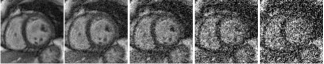
(d) Gaussian noise.

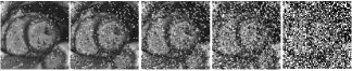
(e) Impulsive noise.

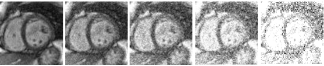
(f) Rician noise.

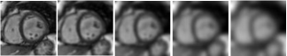
(g) Gaussian blur.

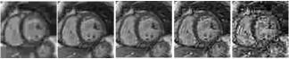
(h) JPEG compression.

Figure 7: Visual examples of input perturbations under various intensity levels. We do not show the examples of adversarial attacks as they are generally imperceptible to the human eye.

4 Experiments

In this section, we first describe the experimental setup, including the dataset and the training and evaluation procedures. We then present the accuracy results and provide a comprehensive comparison of the robustness of LV quantification methods to input perturbations. We last perform a series of ablation experiments to verify that deliberate incorporation of SPT enables robust LV quantification.

4.1 Experimental Setup

Dataset. We use the Cardiac-DIG dataset built by Xue et al. [5], which contains CMR data from $145$ patients. The included examples contain a variety of pathologies, such as myocardial hypertrophy, atrial septal defect, LV dysfunction, etc. Each patient contributes to $20$ mid-cavity, short-axis CMR slices, resulting in a total of $145\times 20=2,900$ images. For each image, two boundaries, the epicardium and endocardium, are manually delineated, based on which the cavity and myocardium areas, three directional dimensions, and six regional wall thicknesses can be accurately computed.

Training and Evaluation Procedure. Training is carried out by minimizing Eq. (3.3) with $\lambda=10^{-3}$ using Adam optimizer. We set the initial learning rate to $4\times 10^{-4}$, and decay it by multiplying $0.12$ whenever the loss plateaus. The minibatch size is $60$, containing CMR data from three subjects. We apply standard data augmentation tricks that are widely used in training CNN-based LV quantification methods, including cropping followed by random zero padding, translation, rotation, and contrast adjustment.

We adopt the MAE and Pearson correlation coefficient $\rho$ as the accuracy metrics, and Robustness Ratio $R$ as the robustness metrics. Note that $\rho$ is computed across subjects: a global correlation between model predictions and human annotations is computed. We use five-fold cross-validation, which divides the whole set equally into five groups, each with $29$ subjects. Four groups of samples are used for training ($70\%$, $101$ subjects) and validation ($10\%$, $15$ subjects), and the last group is used for testing ($20\%$, $29$ subjects). The mean results are reported. The PyTorch implementations are made available at https://github.com/yangyangyang127/LVquant.

Table 1: Accuracy comparison of the proposed method against existing ones in terms of MAE and Pearson correlation

Method		DCAE [5]	DMTRL [6]	Jang18 [23]	Yang18 [24]	Xue20 [51]	Xue20-MD [51]	Yu21 [52]	Ours
Area	$A_{1}$	223±193 0.853	189±159 0.947	207±174 0.874	219±168 -	366±300 -	199±160 -	176±189 -	207±182 0.863
	$A_{2}$	185±162 0.953	172±148 0.943	170±147 0.956	175±126 -	303±248 -	139±111 -	160±158 -	149±122 0.969
	Average	204±133 0.903	180±118 0.945	188±162 -	197±147 0.935	334.5±210 -	169±105 -	168±130 -	178±114 0.955
Dimension	$D_{1}$	-	2.47±1.95 0.957	2.55±2.08 0.937	2.43±1.94 -	3.79±2.96 -	2.01±1.59 -	2.35±1.87 -	2.01±1.66 0.946
	$D_{2}$	-	2.59±2.07 0.854	2.16±1.85 0.958	2.52±1.99 -	3.76±3.48 -	2.38±1.62 -	2.27±2.32 -	2.42±1.9 0.964
	$D_{3}$	-	2.48±2.34 0.943	2.56±2.08 0.941	2.76±2.09 -	4.04±3.14 -	2.46±1.60 -	2.46±2.03 -	2.38±1.92 0.951
	Average	-	2.51±1.58 0.925	2.42±2.01 -	2.57±2.00 0.921	3.86±2.67 -	2.28±1.29 -	2.36±1.45 -	2.27±1.38 0.968
Wall Thickness	$T_{1}$	1.39±1.13 0.824	1.26±1.04 0.856	1.33±1.11 0.843	1.55±1.11 -	2.26±1.89 -	1.31±1.01 -	1.21±1.11 -	1.31±1.11 0.838
	$T_{2}$	1.51±1.21 0.701	1.40±1.10 0.747	1.37±1.12 0.754	1.45±1.12 -	2.22±1.78 -	1.36±1.03 -	1.25±1.17 -	1.6±1.28 0.641
	$T_{3}$	1.65±1.36 0.671	1.59±1.29 0.693	1.62±1.33 0.668	1.59±2.22 -	2.82±2.21 -	1.47±1.21 -	1.50±1.45 -	1.58±1.25 0.591
	$T_{4}$	1.53±1.25 0.698	1.57±1.34 0.659	1.58±1.36 0.644	1.56±1.20 -	2.60±2.09 -	1.53±1.24 -	1.45±1.23 -	1.41±1.24 0.605
	$T_{5}$	1.30±1.12 0.781	1.32±1.10 0.777	1.33±1.19 0.775	1.40±0.99 -	1.99±1.74 -	1.22±1.05 -	1.34±1.19 -	1.78±1.4 0.609
	$T_{6}$	1.28±1.0 0.871	1.25±1.01 0.877	1.30±1.06 0.87	1.52±1.13 -	2.15±1.58 -	1.22±0.94 -	1.23±1.20 -	1.44±1.21 0.824
	Average	1.44±0.71 0.758	1.39±0.68 0.768	1.42±1.21 -	1.51±1.13 0.805	2.34±1.08 -	1.35±0.66 -	1.33±0.82 -	1.52±0.74 0.851

4.2 LV Quantification Accuracy

We compare the proposed method with seven existing methods DCAE [5], DMTRL [6], Jang18 [23], Yang18 [24], Xue20 [51], Xue20-MD [51], and Yu21 [52]. Table 1 shows the quantification accuracy results. We find that our model achieves an average MAE of $178\pm 114$ $\mathrm{mm}^{2}$, $2.27\pm 1.38$ mm, and $1.52\pm 0.74$ mm for LV areas, directional dimensions, and regional wall thicknesses, respectively, which are comparable to the state-of-the-art approaches in the table. DMTRL [6] seeks to learn deep representation and index correlation simultaneously, which outperforms DCAE [5], Jang18 [23], and Yang18 [24]. Xue20-MD [51] ensembles the results of Monte Carlo dropout models, and Yu21  [52] leverages computed tomography (CT) information, both of which make progress in accuracy. Moreover, the proposed method achieves an average Pearson correlation of $0.955$, $0.968$, and $0.851$ for area, dimension, and thickness predictions, respectively, all surpassing existing approaches.

We show in Fig. 8 the comparison between the mean of estimated and true values of the LV indices in a cardiac cycle. It can be seen that our method keeps an accurate track of all LV indices, indicating that the spatiotemporal dynamics of the LV are adequately modeled.

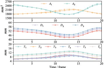
Figure 8: Comparison between the mean of predicted (dashed line) and true LV index values (solid line) in a cardiac cycle.

4.3 Quantification Robustness

We show the robustness results, $R$, to spatial transformations, image distortions, and adversarial attacks in Figs. 9, 10, and 11, respectively. For neat presentation, we calculate the average $R$ of the two areas, three dimensions, and six thicknesses, respectively. From the comparison with existing approaches, we have several interesting observations. First, it is clear that the SPT-augmented method shows significantly improved robustness to translation, and is fairly stable under rotation. Despite being blind to the five image distortions, the proposed method is able to make reliable LV quantification and performs remarkably well under Gaussian and Rician noise. Interestingly, we find that our method provides more robust predictions of regional wall thicknesses ($\{T_{i}\}$) compared to cavity/myocardium areas ($\{A_{i}\}$) and directional dimensions ($\{D_{i}\}$). We conjecture this arises because $\{T_{i}\}$ are local indices, which require less global structural information and thus are less affected by image distortions. Third, although we do not employ adversarial training, the resulting method is reasonably resistant to $50$-iteration adversarial attacks and degrades under $100$-iteration attacks, indicating that our method does not suffer from gradient obfuscation, a frequently occurred pitfall when evaluating adversarial robustness. As will be clear in Sec. 4.4, the observed adversarial robustness may not be the sole result of the SPT as front-end processing, but the combination effect of SPT and LSTM.

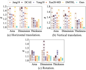
Figure 9: Robustness of LV quantification methods to spatial transformations in terms of the average ratio of MAEs (see Eq. (12)). A larger dot represents a severer intensity level.

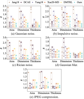
Figure 10: Robustness of LV quantification methods to image distortions.

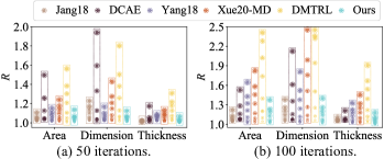
Figure 11: Robustness of LV quantification methods to adversarial attacks.

4.4 Ablation Studies

To obtain a deeper understanding of the robustness of our SPT-augmented method, we design a thorough set of ablation experiments to verify that the main source of robustness is indeed from SPT.

We train several degenerated variants of our default model, for which we intentionally exclude LSTM for temporal modeling and correlation constraints for regularization. All variants are trained without data augmentation unless otherwise mentioned. The detailed specifications of the variants along with their acronyms are given in Table 2. Baseline is a generic CNN that takes a CMR slice as input and directly regresses the eleven indices. Baseline-Aug is built on top of Baseline by adding the data augmentation described in Sec. 4.1. SPT-AC decomposes the CMR slice into two scales and three orientations, all of which are organized into the channel dimension for the CNN to process. SPT-AC-H and SPT-AC-L rely on SPT-AC, which further add the residual highpass and lowpass subbands into the channel dimension, respectively. SPT-OC-L differs from SPT-AC-L in that the former organizes the orientation subbands (and residual lowpass subband) in the channel dimension and the scale subbands in the batch dimension, enabling parameter sharing across scales. SPT-SC-L is the spatial degenerate of the proposed method, which puts the scale subbands (and residual lowpass subband) in the channel dimension and the orientation subbands in the batch dimension, allowing parameter sharing across orientations.

Through comparison between Baseline, Baseline-Aug, SPT-AC-L, SPT-OC-L, and SPT-SC-L, we are able to identify the role of SPT. From Fig. 12, the primary observation is that incorporation of SPT enables robust LV quantification, especially for image distortions. Second, how to share subbands with respect to the CNN seems important to prediction robustness. The variant that allows CNN parameter sharing across orientations does a good job under various input perturbations. Third, Baseline-Aug is exposed to translated and rotated training data through data augmentation. As expected, it outperforms SPT-based variants under seen translations and rotations. Nevertheless, the SPT variants are also able to boost model robustness under spatial transformations compared to the naïve Baseline. Fourth, all methods in question are vulnerable to adversarial attacks. In contrast to the result in Fig. 11, we conclude that the adversarial robustness of our method mainly arises from the combination of LSTM and SPT.

Comparison between SPT-AC, SPT-AC-H, and SPT-AC-L in Fig. 13 reveals the effect of the residual highpass and lowpass subbands in SPT. We find that adding the lowpass subband improves the robustness for the majority of input perturbations. By comparing SPT-AC-L and SPT-SC-L, we see that simply eliminating the highpass subband does not seem to work well; it is the multi-scale and multi-orientation representation that leads to robustness. This verifies our design choice of including lowpass subband and excluding highpass subband in SPT.

Table 2: Variants of the proposed method. “H” and “L” denote residual highpass and lowpass subbands, respectively. The input shape is in the form of “batch$\times$ channel $\times$ height $\times$ Width”

Variant	Whether to Use SPT	# of SPT Scales / Orientations	Whether to Use H and L	Whether to Use Data Augmentation	Input Shape	Output Shape
Baseline	✗	N.A.	N.A.	✗	$1\times 80\times 80$	$11\times 1$
Baseline-Aug	✗	N.A.	N.A.	✓	$1\times 80\times 80$	$11\times 1$
SPT-AC	✓	2 / 3	✗	✗	$6\times 80\times 80$	$11\times 1$
SPT-AC-H	✓	2 / 3	H	✗	$7\times 80\times 80$	$11\times 1$
SPT-AC-L	✓	2 / 3	L	✗	$7\times 80\times 80$	$11\times 1$
SPT-OC-L	✓	2 / 3	L	✗	$3\times 3\times 80\times 80$	$11\times 3$
SPT-SC-L	✓	2 / 3	L	✗	$3\times 3\times 80\times 80$	$5\times 3$

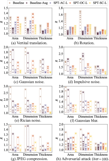
Figure 12: Robustness test of LV quantification variants of the proposed method to identify the role of SPT.

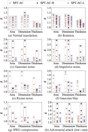
Figure 13: Robustness test of LV quantification variants to identify the role of highpass and lowpass subbands.

5 Conclusion

We have proposed a robust LV quantification method by incorporating SPT as fixed front-end processing. Our method delivers accurate LV quantification results, and is robust to various input perturbations. We hope our work can draw the community’s attention to the robustness aspects of computer-aided diagnosis, which is of great practical importance. The proposed usage of SPT may also be beneficial for other medical applications that are scale- and orientation-dependent, which are worth exploring in future.

References

- [1] S. Mendis, P. Puska, and B. Norrving, Global Atlas on Cardiovascular Disease Prevention and Control. World Health Organization, 2011.
- [2] P. Peng, K. Lekadir, A. Gooya, L. Shao, S. Petersen, and A. Frangi, “A review of heart chamber segmentation for structural and functional analysis using cardiac magnetic resonance imaging,” Magnetic Resonance Materials in Physics and Biology and Medicine, vol. 29, no. 2, pp. 155–195, 2016.
- [3] F. Grothues, G. Smith, J. C. Moon, N. G. Bellenger, P. L. Collins, H. U. Klein, and D. J. Pennell, “Comparison of interstudy reproducibility of cardiovascular magnetic resonance with two-dimensional echocardiography in normal subjects and in patients with heart failure or left ventricular hypertrophy,” The American Journal of Cardiology, vol. 90, pp. 29–34, 2002.
- [4] F. Grothues, J. C. Moon, N. G. Bellenger, G. S. Smith, H. U. Klein, and D. J. Pennell, “Interstudy reproducibility of right ventricular volumes, function, and mass with cardiovascular magnetic resonance,” American Heart Journal, vol. 147, no. 2, pp. 218–223, 2004.
- [5] W. Xue, A. Islam, M. Bhaduri, and S. Li, “Direct multitype cardiac indices estimation via joint representation and regression learning,” IEEE Transaction on Medical Imaging, vol. 36, no. 10, pp. 2057–2067, 2017.
- [6] W. Xue, G. Brahm, S. Pandey, S. Leung, and S. Li, “Full left ventricle quantification via deep multitask relationships learning,” Medical Image Analysis, vol. 43, pp. 54–65, 2018.
- [7] X. Ma, Y. Niu, L. Gu, Y. Wang, Y. Zhao, J. Bailey, and F. Lu, “Understanding adversarial attacks on deep learning based medical image analysis systems,” Pattern Recognition, vol. 110, no. 107332, pp. 1–11, 2021.
- [8] E. P. Simoncelli and W. T. Freeman, “The steerable pyramid: A flexible architecture for multi-scale derivative computation,” in IEEE International Conference on Image Processing, vol. 3, pp. 444–447, 1995.
- [9] H. Wang, X. Wu, Z. Huang, and E. P. Xing, “High-frequency component helps explain the generalization of convolutional neural networks,” in IEEE Conference on Computer Vision and Pattern Recognition, pp. 8684–8694, 2020.
- [10] W. Bai, W. Shi, H. Wang, N. Peters, and D. Rueckert, “Multi-atlas based segmentation with local label fusion for right ventricle MR images,” in International Conference on Medical Image Computing and Computer-Assisted Intervention RV Segmentation Challenge, pp. 1–8, 2012.
- [11] Y. Ou, J. Doshi, G. Erus, and C. Davatzikos, “Multi-atlas segmentation of the cardiac MR right ventricle,” in International Conference on Medical Image Computing and Computer-Assisted Intervention RV Segmentation Challenge, pp. 1–8, 2012.
- [12] J. Duan, G. Bello, J. Schlemper, W. Bai, T. Dawes, C. Biffi, A. Marvao, G. Doumoud, D. O’Regan, and D. Rueckert, “Automatic 3D bi-ventricular segmentation of cardiac images by a shape-refined multi-task deep learning approach,” IEEE Transactions on Medical Imaging, vol. 38, no. 9, pp. 2151–2164, 2019.
- [13] J. Long, E. Shelhamer, and T. Darrell, “Fully convolutional networks for semantic segmentation,” in IEEE Conference on Computer Vision and Pattern Recognition, pp. 3431–3440, 2015.
- [14] O. Ronneberger, P. Fischer, and T. Brox, “U-Net: Convolutional networks for biomedical image segmentation,” in International Conference on Medical Image Computing and Computer-Assisted Intervention, pp. 234–241, 2015.
- [15] S. Ji, W. Xu, M. Yang, and K. Yu, “3D convolutional neural networks for human action recognition,” IEEE Transactions on Pattern Analysis and Machine Intelligence, vol. 35, no. 1, pp. 221–231, 2012.
- [16] J. Yan, Y. Zhong, Y. Fang, Z. Wang, and K. Ma, “Exposing semantic segmentation failures via maximum discrepancy competition,” International Journal of Computer Vision, vol. 129, no. 5, pp. 1768–1786, 2021.
- [17] H. Wang, T. Chen, Z. Wang, and K. Ma, “I am going MAD: Maximum discrepancy competition for comparing classifiers adaptively,” in International Conference on Learning Representations, pp. 1–12, 2020.
- [18] X. Zhen, Z. Wang, A. Islam, M. Bhaduri, I. Chan, and S. Li, “Direct estimation of cardiac bi-ventricular volumes with regression forests,” in International Conference on Medical Image Computing and Computer-Assisted Intervention, pp. 586–593, 2014.
- [19] Z. Wang, M. Salah, B. Gu, A. Islam, G. Aashish, and S. Li, “Direct estimation of cardiac biventricular volumes with an adapted Bayesian formulation,” IEEE Transactions on Biomedical Engineering, vol. 61, no. 4, pp. 1251–1260, 2014.
- [20] X. Zhen, A. Islam, M. Bhaduri, I. Chan, and S. Li, “Direct and simultaneous four-chamber volume estimation by multi-output regression,” in International Conference on Medical Image Computing and Computer-Assisted Intervention, pp. 669–676, 2015.
- [21] S. E. Petersen, P. M. Matthews, J. M. Francis, M. D. Robson, F. Zemrak, R. Boubertakh, A. A. Young, S. Hudson, P. Weale, S. Garratt, R. Collins, S. Piechnik, and S. Neubauer, “UK Biobank’s cardiovascular magnetic resonance protocol,” Journal of Cardiovascular Magnetic Resonance, vol. 18, no. 1, pp. 1–7, 2015.
- [22] O. Bernard, A. Lalande, C. Zotti, F. Cervenansky, X. Yang, P. Heng, I. Cetin, K. Lekadir, O. Camara, M. Ballester, G. Sanroma, S. Napel, S. Petersen, G. Tziritas, E. Grinias, M. Khened, V. Kollerathu, G. Krishnamurthi, M. Rohé, X. Pennec, M. Sermesant, F. Isensee, P. Jager, K. Maier-Hein, P. Full, I. Wolf, S. Engelhardt, C. Baumgartner, L. Koch, J. Wolterink, I. Isgum, Y. Jang, Y. Hong, J. Patravali, S. Jain, O. Humbert, and P. Jodoin, “Deep learning techniques for automatic MRI cardiac multi-structures segmentation and diagnosis: Is the problem solved?” IEEE Transactions on Medical Imaging, vol. 37, no. 11, pp. 2514–2525, 2018.
- [23] Y. Jang, S. Kim, H. Shim, and H. J. Chang, “Full quantification of left ventricle using deep multitask network with combination of 2D and 3D convolution on 2D + t cine MRI,” in International Workshop on Statistical Atlases and Computational Models of the Heart. Atrial Segmentation and LV Quantification Challenges, pp. 476–483, 2018.
- [24] G. Yang, T. Hua, C. Lu, T. Pan, X. Yang, L. Hu, J. Wu, X. Zhu, and H. Shu, “Left ventricle full quantification via hierarchical quantification network,” in International Workshop on Statistical Atlases and Computational Models of the Heart. Atrial Segmentation and LV Quantification Challenges, pp. 429–438, 2018.
- [25] E. P. Simoncelli, W. T. Freeman, E. H. Adelson, and D. J. Heeger, “Shiftable multiscale transforms,” IEEE Transactions on Information Theory, vol. 38, no. 2, pp. 587–607, 1992.
- [26] J. Portilla, V. Strela, M. J. Wainwright, and E. P. Simoncelli, “Image denoising using scale mixtures of Gaussians in the wavelet domain,” IEEE Transactions on Image Processing, vol. 12, no. 11, pp. 1338–1351, 2003.
- [27] R. W. Buccigrossi and E. P. Simoncelli, “Image compression via joint statistical characterization in the wavelet domain,” IEEE Transactions on Image Processing, vol. 8, no. 12, pp. 1688–1701, 1999.
- [28] S. Lyu and H. Farid, “Steganalysis using higher-order image statistics,” IEEE Transactions on Information Forensics and Security, vol. 1, no. 1, pp. 111–119, 2006.
- [29] H. R. Sheikh and A. C. Bovik, “Image information and visual quality,” IEEE Transactions on Image Processing, vol. 15, no. 2, pp. 430–444, 2006.
- [30] J. Portilla and E. P. Simoncelli, “A parametric texture model based on joint statistics of complex wavelet coefficients,” International Journal of Computer Vision, vol. 40, no. 1, pp. 49–70, 2000.
- [31] J. Chen, T. N. Pappas, A. Mojsilovic, and B. E. Rogowitz, “Adaptive perceptual color-texture image segmentation,” IEEE Transactions on Image Processing, vol. 14, no. 10, pp. 1524–1536, 2005.
- [32] A. D. Jepson, D. J. Fleet, and T. F. El-Maraghi, “Robust online appearance models for visual tracking,” IEEE Transactions on Pattern Analysis and Machine Intelligence, vol. 25, no. 10, pp. 1296–1311, 2003.
- [33] S. Meyer, A. Djelouah, B. McWilliams, A. Sorkine-Hornung, M. Gross, and C. Schroers, “PhaseNet for video frame interpolation,” in IEEE Conference on Computer Vision and Pattern Recognition, pp. 498–507, 2018.
- [34] S. Bhardwaj, I. Fischer, J. Ballé, and T. Chinen, “An unsupervised information-theoretic perceptual quality metric,” arXiv preprint arXiv:2006.06752, 2021.
- [35] D. Deng, Z. Chen, Y. Zhou, and B. Shi, “MIMAMO Net: Integrating micro-and macro-motion for video emotion recognition,” in AAAI Conference on Artificial Intelligence, pp. 2621–2628, 2020.
- [36] N. Parthasarathy and E. P. Simoncelli, “Self-supervised learning of a biologically-inspired visual texture model,” arXiv preprint arXiv:2006.16976, 2020.
- [37] X. Shi, Z. Chen, H. Wang, D. Y. Yeung, W. K. Wong, and W. Woo, “Convolutional LSTM network: A machine learning approach for precipitation nowcasting,” in Advances in Neural Information Processing Systems, pp. 802–810, 2015.
- [38] B. Awasthi, J. Friedman, and M. A. Williams, “Faster, stronger, lateralized: Low spatial frequency information supports face processing,” Neuropsychologia, vol. 49, no. 13, pp. 3583–3590, 2011.
- [39] M. Bar, “Visual objects in context,” Nature Reviews Neuroscience, vol. 5, no. 8, pp. 617–629, 2004.
- [40] D. Yin, R. Lopes, J. Shlens, E. D. Cubuk, and J. Gilmer, “A Fourier perspective on model robustness in computer vision,” arXiv preprint arXiv:1906.08988, 2019.
- [41] M. Cerqueira, N. Weissman, V. Dilsizian, A. Jacobs, S. Kaul, W. Laskey, D. Pennell, J. Rumberger, T. Ryan, and M. Verani, “Standardized myocardial segmentation and nomenclature for tomographic imaging of the heart: A statement for healthcare professionals from the Cardiac Imaging Committee of the Council on Clinical Cardiology of the American Heart Association,” Circulation, vol. 105, no. 4, pp. 539–542, 2002.
- [42] M. Ohlson, M. Ahmad, and D. Rosen, “The multilinear normal distribution: Introduction and some basic properties,” Journal of Multivariate Analysis, vol. 113, pp. 37–47, 2013.
- [43] A. Azulay and Y. Weiss, “Why do deep convolutional networks generalize so poorly to small image transformations?” arXiv preprint arXiv:1805.12177, 2018.
- [44] S. Vaseghi, Advanced Signal Processing and Digital Noise Reduction. Vieweg+Teubner Verlag, 1996.
- [45] P. Coupe, J. Manjon, E. Gedamu, D. Arnold, M. Robles, and L. Collins, “Robust Rician noise estimation for MR images,” Medical Image Analysis, vol. 14, no. 4, pp. 483–493, 2010.
- [46] L. He and I. Greenshields, “A nonlocal maximum likelihood estimation method for Rician noise reduction in MR images,” IEEE Transactions on Medical Imaging, vol. 28, no. 2, pp. 165–172, 2008.
- [47] D. Hendrycks and T. Dietterich, “Benchmarking neural network robustness to common corruptions and perturbations,” arXiv preprint arXiv:1903.12261, 2019.
- [48] I. Goodfellow, J. Shlens, and C. Szegedy, “Explaining and harnessing adversarial examples,” arXiv preprints arXiv:1412.6572, 2014.
- [49] A. Madry, A. Makelov, L. Schmidt, D. Tsipras, and A. Vladu, “Towards deep learning models resistant to adversarial attacks,” arXiv preprints arXiv:1706.06083, 2017.
- [50] S. Gu and L. Rigazio, “Towards deep neural network architectures robust to adversarial examples,” arXiv preprints arXiv:1412.5068, 2014.
- [51] W. Xue, T. Guo, and D. Ni, “Left ventricle quantification with sample-level confidence estimation via Bayesian neural network,” Computerized Medical Imaging and Graphics, vol. 84, no. 101753, pp. 1–7, 2020.
- [52] C. Yu, Z. Gao, W. Zhang, G. Yang, S. Zhao, H. Zhang, Y. Zhang, and S. Li, “Multitask learning for estimating multitype cardiac indices in MRI and CT based on adversarial reverse mapping,” IEEE Transactions on Neural Networks and Learning Systems, vol. 32, no. 2, pp. 493–506, 2021.