MeMViT: Memory-Augmented Multiscale Vision Transformer
for Efficient Long-Term Video Recognition

Abstract

While today’s video recognition systems parse snapshots or short clips accurately, they cannot connect the dots and reason across a longer range of time yet. Most existing video architectures can only process $<$5 seconds of a video without hitting the computation or memory bottlenecks.

In this paper, we propose a new strategy to overcome this challenge. Instead of trying to process more frames at once like most existing methods, we propose to process videos in an online fashion and cache “memory” at each iteration. Through the memory, the model can reference prior context for long-term modeling, with only a marginal cost. Based on this idea, we build MeMViT, a Memory-augmented Multiscale Vision Transformer, that has a temporal support 30$\times$longer than existing models with only 4.5% more compute; traditional methods need $>$3,000% more compute to do the same. On a wide range of settings, the increased temporal support enabled by MeMViT brings large gains in recognition accuracy consistently. MeMViT obtains state-of-the-art results on the AVA, EPIC-Kitchens-100 action classification, and action anticipation datasets. Code and models are available at https://github.com/facebookresearch/memvit.

1 Introduction

Our world evolves endlessly over time. The events at different points in time influence each other and all together, they tell the story of our visual world. Computer vision promises to understand this story, but today’s systems are still quite limited. They accurately parse visual content in independent snapshots or short time periods (e.g., 5 seconds), but not beyond that. So, how can we enable accurate long-term visual understanding? There are certainly many challenges ahead, but having a model that practically runs on long videos is arguably an important first step.

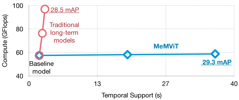
(a)

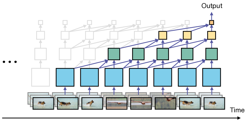
(b)

Figure 1: MeMViT is a class of video models that models long videos efficiently. It has a significantly better trade-off than traditional methods, which increase the temporal support of a video model by increasing the number of frames in model input (Fig. LABEL:fig:teaser:a). MeMViT achieves efficient long-term modeling by hierarchically attending the previously cached “memory” of the past (Fig. LABEL:fig:teaser:b).

In this paper, we propose a memory-based approach for building efficient long-term models. The central idea is that instead of aiming to jointly process or train on the whole long video, we simply maintain “memory” as we process a video in an online fashion. At any point of time, the model has access to prior memory for long-term context. Since the memory is ‘reused’ from the past, the model is highly efficient. To implement this idea, we build a concrete model called MeMViT, a Memory-augmented Multiscale Vision Transformer. MeMViT processes 30$\times$ longer input duration than existing models, with only 4.5% more compute. In comparison, a long-term model built by increasing the number of frames will require $>$3,000% more compute. Fig. LABEL:fig:teaser:a presents the trade-off comparison in compute/duration.

More concretely, MeMViT uses the “keys” and “values” of a transformer [74] as memory. When the model runs on one clip, the “queries” attend to an extended set of “keys” and “values”, which come from both the current time and the past. When performing this at multiple layers, each layer attends further down into the past, resulting in a significantly longer receptive field, as illustrated in Fig. LABEL:fig:teaser:b.

To further improve the efficiency, we jointly train a memory compression module for reducing the memory footprint. Intuitively, this allows the model to learn which cues are important for future recognition and keeps only those.

Our design is loosely inspired by how humans parse long-term visual signals. Humans do not process all signals over a long period of time at once. Instead, humans process signals in an online fashion, associate what we see to past memory to make sense of it, and also memorize important information for future use.

Our results demonstrate that augmenting video models with memory and enabling long range attention is simple and very beneficial. On the AVA spatiotemporal action localization [32], the EPIC-Kitchens-100 action classification [13, 14], and the EPIC-Kitchens-100 action anticipation datasets [13, 14], MeMViT obtains large performance gains over its short-term counterpart and achieves state-of-the-art results. We hope these results are helpful for the community and take us one step closer to understanding the interesting long story told by our visual world.

2 Related Work

Video understanding models

aim to parse spatiotemporal information in videos. Popular approaches in the past decade include the classic works that use handcrafted features [20, 16, 36, 12, 39, 77, 76, 75, 55], recurrent networks [34, 17, 52, 42, 45, 65], and 2D- [79, 85, 78] or 3D-CNNs [69, 72, 4, 24, 23, 90, 45, 73, 56, 45, 87, 81, 27]. More recently, methods built upon the Transformer [74] architecture (the vision transformers) have been shown promising results [22, 2, 54, 51, 3].

Vision transformers

[19, 22, 49, 2, 18, 70, 88, 71, 31] treat an image as a set of patches and model their interactions with transformer-based architectures [74]. Recent works adding vision priors such as multi-scale feature hierarchies [22, 31, 49, 80, 88] or local structure modeling [49, 18, 9] have shown to be effective. They have also been generalized from the image to video domain [22, 3, 51, 54]. In this work, we build our architecture based on the Multiscale Vision Transformer (MViT) architecture [22, 44] as a concrete instance, but the general idea can be applied to other ViT-based video models.

Long-term video models

aim to capture longer-term patterns in long videos (e.g., $>$30 seconds). To reduce the high computational cost, one widely studied line of work directly models pre-computed features without jointly training backbones [1, 89, 84, 17, 29]. Another potential direction designs efficient models [92, 38, 85, 46, 33, 90] to make covering more frames feasible. More related to our work is the less-studied middle ground that builds a memory-like design that still allows for end-to-end training but has greatly reduced overhead [83, 41, 40, 8]. For example, ‘long-term feature bank’-based methods extend standard video backbones to reference long-term supportive context features [83, 53]. However, these methods capture only final-layer features and require two backbones, two rounds of training and inference computation. MeMViT flexibly models features at arbitrary layers with minimal changes to standard training methods and only requires one standalone backbone.

Online video modeling

arises naturally in applications such as robotics, AR/VR, or video streaming. While one may use an image-based method (e.g., [60]) to parse a video frame-by-frame, to consider longer-term context, most existing works use causal convolutions [6, 37, 10], RNNs [17, 48], or feature fusion [91, 8]. In this work, we explore attention-based designs, which directly reference arbitrary points of time in the past, without the need to fight forgetfulness as in RNNs or being constrained by kernel size as in CNNs.

Transformer designs in NLP

are also related to our method. MeMViT takes inspiration from long-range language models [11, 58, 63, 64, 59], which also cache long-range “memory”. Different from these works, video models process significantly larger tensors ($T{\times}W{\times}H$), making caching and attending memory expensive if not prohibitive. Prior work in NLP attempts to learn a module to compress memory, but the requirement of backpropagation through time (BPTT) makes it challenging [58]. Rae et al. [58] thus uses autoencoder for memory compression, but that cannot be optimized for the end task. In this paper, we present a “pipelined” memory compression method that is efficient and end-to-end optimizable for the end task, without BPTT.

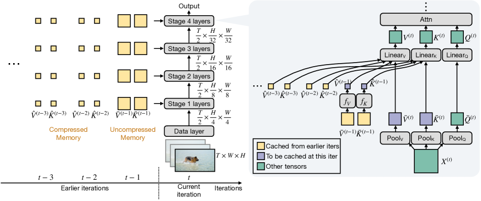
Figure 2: MeMViT is a memory-augmented mulstiscale vision transformer network for long-term video recognition. MeMViT treats a long video as a sequence of short clips and process them sequentially. (Consecutive iterations see consecutive clips.) “Memory” obtained from earlier iterations were cached, so that MeMViT processing the current clip can reference the memory. Note that at the current iteration we cache the uncompressed memory, which will only be compressed at the next iteration. See text for details. Left: Model overview. Right: Detailed MeMViT attention design.

3 Preliminaries

In this paper, we build MeMViT based on the MViT [22, 44] architecture due to its strong performance, but the techniques presented in this paper can be applied to other ViT-based architectures. For completeness, we review ViT and MViT and introduce notations used in this paper next.

Vision Transformers (ViT)

first embeds an image into $N$ non-overlapping patches (using a strided convolution) and packs them into a tensor $X^{0}\in\mathbb{R}^{N\times d}$. A stack of transformer layers then models the interactions among these patches. The central component of a transformer layer is the attention operation, which first linearly projects an input tensor $X$ to be queries $Q$, keys $K$, and values $V$:

$$Q=XW_{Q},\quad K=XW_{K},\quad V=XW_{V},$$ (1)

and performs a self-attention operation

$$Z:=\mathrm{Attn}(Q,K,V)=\mathrm{Softmax}\left(QK^{\top}/\sqrt{d}\right)V,$$ (2)

to obtain an output tensor $Z\in\mathbb{R}^{N\times d_{\textrm{out}}}$.

Multiscale Vision Transformers (MViT)

improves ViT based on two simple ideas. First, instead of having a fixed resolution of $N$ throughout the network, MViT learns multi-scale representations through multiple stages, starting from fine-grained modeling of smaller patches (with large $N$ and small $d$) to high-level modeling of larger patches in later stages (with small $N$ and large $d$). The transition between stages is done through strided pooling. Second, MViT uses pooling attention ($\mathcal{P}$) that pools spatiotemporal dimensions of $Q$, $K$, and $V$ to drastically reduce computational cost of an attention layer, i.e.,

$$Q=\mathcal{P}_{Q}\left(XW_{Q}\right),\ K=\mathcal{P}_{K}\left(XW_{K}\right),\ V=\mathcal{P}_{V}\left(XW_{V}\right).$$

These two changes significantly improve the model performance and efficiency. In this paper, we build our method based on a slightly modified MViT, where we swap the order of linear layer and pooing:

$$\bar{Q}=\mathcal{P}_{Q}\left(X\right),\quad\bar{K}=\mathcal{P}_{K}\left(X\right),\quad\bar{V}=\mathcal{P}_{V}\left(X\right)$$ (3)

$$Q=\bar{Q}W_{Q},\quad K=\bar{K}W_{K},\quad V=\bar{V}W_{V}\quad$$ (4)

This allows the linear layer to operate on smaller tensors, reducing the computational cost without affecting accuracy. See the Appendix for an ablation study on this change. In the next section, we will see how this change also makes MeMViT more efficient.

To build longer duration video models, most state-of-the-art methods simply increase the number of frames in the input clip [81, 24, 22]. This strategy increases the computational cost significantly. In the next section, we present our method for building more efficient long-term video models.

4 MeMViT for Efficient Long-Term Modeling

Our method is simple. We split a video into a sequence of short $T\times H\times W$ clips and process them sequentially (for both training and inference). Consecutive iterations see consecutive clips. We cache “memory”, some representations of the processed clip, at each iteration. When processing the current clip at time step $t$, the model has access to previously cached ‘memory’ from earlier iterations $t^{\prime}<t$ for long-term context. Fig. 2 shows an overview.

4.1 Memory Attention and Caching

The Basic MeMViT Attention.

One simple way to implement this idea is to treat the “keys” $\bar{K}$ and “values” $\bar{V}$ in the transformer architecture as a form of memory, and extend $\bar{K}^{(t)}$ and $\bar{V}^{(t)}$ at current iteration $t$ to include $\bar{K}^{(t^{\prime})}$ and $\bar{V}^{(t^{\prime})}$ cached from earlier iterations $t^{\prime}$ from $t-M$ to $t-1$, i.e.,

$$\bar{K}^{(t)} :=\left[\mathrm{sg}\left(\bar{K}^{(t-M)}\right),\ldots,\mathrm{sg}\left(\bar{K}^{(t-1)}\right),\bar{K}^{(t)}\right],$$ (5)

$$\bar{V}^{(t)} :=\left[\mathrm{sg}\left(\bar{V}^{(t-M)}\right),\ldots,\mathrm{sg}\left(\bar{V}^{(t-1)}\right),\bar{V}^{(t)}\right],$$ (6)

where the square brackets denote concatenation along the token dimension. With this formulation, the query $Q$ attends not only information about the current time step $t$, but also information from up to $M$ steps before. Here, the “stop gradient” operator ($\mathrm{sg}$) breaks further dependency into the past in backpropagation. Note that the memory is built hierarchically over time (see Fig. LABEL:fig:teaser:b) and our previous key and value memory holds information stored from prior time-steps.

The additional cost for training and inference encompasses only the GPU memory for memory caching and the extra compute in the extended attention layer. All other parts of the network (MLPs, etc.) remain unchanged. The cost grows with temporal support in $\mathcal{O}\left(M\right)$, instead of $\mathcal{O}\left(T^{2}\right)$ as in traditional scaling methods.

In this basic implementation, we cache the full key and value tensors, which may contain redundant information that is not useful for future recognition. In the next section we will discuss methods to compress memory for keeping only ‘important’ information.

Algorithm 1 Pseudocode of MeMViT attention in a PyTorch-like style.

⬇

class MeMViTAttention():

# pool_q, pool_k, pool_v: pooling layers

# lin_q, lin_k, lin_v: linear layers

# f_k, f_v: compression modules

self.m_k = [] # cached memory keys

self.m_v = [] # cached memory values

self.max_len # max memory length

def forward(x):

# compute the pooled Q, K, and V

q, k, v = pool_q(x), pool_k(x), pool_v(x)

# compress memory

cm_k = f_k(m_k[-1])

cm_v = f_v(m_v[-1])

# perform attention on augmented keys and values

z = attn(

lin_q(q),

lin_k(cat(self.m_k[:-1] + [cm_k, k])),

lin_v(cat(self.m_v[:-1] + [cm_v, v])),

)

# cache newly compressed memory

self.m_k[-1] = cm_k.detach()

self.m_v[-1] = cm_v.detach()

# cache current uncompressed memory

self.m_k.append(k.detach())

self.m_v.append(v.detach())

# maintain max length for memory

if len(self.m_k) > self.max_mem:

self.m_k.pop_first()

self.m_v.pop_first()

return z

  cat: concatenation along token dimension.

4.2 Memory Compression

Naïve Memory Compression.

There are many potential ways to compress the memory, but one intuitive design attempts to jointly train compression modules (e.g., learnable pooling operators), $f_{K}$ and $f_{V}$, to reduce the spatiotemporal size of $K$ and $V$ tensors, respectively:

$$\bar{K}^{(t)}:=\left[f_{K}\left(\mathrm{sg}(\bar{K}^{(t-M)})\right),\ldots,f_{K}\left(\mathrm{sg}(\bar{K}^{(t-1)})\right),\bar{K}^{(t)}\right],$$

and similarly for $\bar{V}^{(t)}$. With this design, we only need to cache and attend the ‘compressed’ memory, $f_{K}\left(\bar{K}^{(t^{\prime})}\right)$ and $f_{V}\left(\bar{V}^{(t^{\prime})}\right)$, at inference time, thus reducing the memory footprint and the computational cost. Nonetheless, at training time, it needs to jointly train on all the ‘full’ memory tensor, thus which may actually increase the memory consumption and cost, making obtaining such a model expensive. The cost is even higher for models with a larger $M$ for longer-term modeling.

(a)

(b)

(c)

(d)

(e)

(f)

Figure 3: Comparison of Scaling Strategies. Scaling with MeMViT obtains significantly better trade-off than alternative strategies in terms of training GPU memory (Fig. LABEL:fig:tradeoff:trmem), inference GPU memory (LABEL:fig:tradeoff:temem), training runtime (LABEL:fig:tradeoff:trtime), inference runtime (LABEL:fig:tradeoff:tetime) and FLOPs (LABEL:fig:tradeoff:flops), while being more accurate (LABEL:fig:tradeoff:map). (The widely used ‘baseline scaling’ strategy increases the temporal support of a video model by increasing the number of frames $T$ in input.) All methods use the same hardware and software implementation.

Pipelined Memory Compression.

To address this issue, we propose a pipelined compression method. Our insight is that while the compression modules $f_{K}$ and $f_{V}$ need to run on uncompressed memory and be jointly optimized, so that the model learns what is important to keep, the learned modules can be shared across all the past memory. Thus, we propose to train to compress memory at only one step at a time, i.e.,

$$\bar{K}^{(t)} :=\left[\hat{K}^{(t-M)},\ldots,\hat{K}^{(t-2)},f_{K}\left(\mathrm{sg}\left(\bar{K}^{(t-1)}\right)\right),\bar{K}^{(t)}\right],$$

and similarly for $\bar{V}^{(t)}$. The right hand side of Fig. 2 illustrates this design. Note that here only the memory $\mathrm{sg}\left(\bar{K}^{(t-1)}\right)$ from the immediate previous step is cached uncompressed, and to be used to train $f_{K}$ in the current iteration. $\hat{K}^{(t^{\prime})}=\mathrm{sg}\left(f_{K}(\bar{K}^{(t^{\prime})})\right)$ for $t^{\prime}$ from $t-M$ to $t-2$ are compressed memory cached from earlier iterations. Algorithm 1 presents the pseudo code for this process.

In this way, MeMViT adds only a ‘constant’ compression cost over the ‘basic’ MeMViT, since it only runs compression on one single step at a time. But, it reduces the caching and attention cost for all other steps drastically (e.g. 16$\times$ by default). In §5, we will show that overall this leads to significant saving, while maintaining high accuracy.

One appealing property of our design is that the receptive field of our video models grows not only with $M$ but also the number of layers $L$, since each layer attends further down into the past, therefore hierarchically increasing the temporal receptive field with depth. See Fig. LABEL:fig:teaser:b for an illustration.

4.3 Implementation Details

Data Loading.

During both training and inference, we perform sequential reading of consecutive chunks of frames (clips) to process videos in an online fashion. This is also the natural setting in a wide range of applications, e.g., robotics or recognition on live streaming video. In our implementation, we simply concatenate all videos and read them sequentially. In cases where the cached memory comes from the previous video (i.e., at the video boundary) we mask the memory to be zero.

Compression Module Design.

The compression module can be any function that reduces the number of tokens but maintains the dimensionality $d$. In our instantiation we choose a learnable pooling [22] due to its simplicity and strong performance, but other choices are possible. We will study the effect of different downsampling factors in §5.2.

Positional Embedding.

In the original MViT [22], absolute positional embeddings are added to the input of the network, and each clip uses the same positional embeddings. Thus the positional embeddings can only indicate the positions within a clip, but not the order across multiple clips. We thus adopt the relative positional embedding used in “the improved MViT” [44], so that memory at different points in time has a different relative distance to the queries.

Mem len	Receptive field	GFLOPs	mAP
w/o mem	1$\times$	57.4	27.0
1	8$\times$	58.1	28.7
2	16$\times$	58.7	29.3
3	24$\times$	59.3	29.2
4	32$\times$	60.0	28.8

(a)

Compress factor	GFLOPs	mAP
none	73.0	28.9
1$\times$2$\times$2	62.3	29.0
2$\times$1$\times$1	65.3	29.1
2$\times$2$\times$2	59.9	29.0
2$\times$4$\times$4	58.2	28.3
4$\times$2$\times$2	58.7	29.3
4$\times$4$\times$4	57.8	28.6

(b)

Aug layers	GFLOPs	mAP
all	60.2	29.1
75% (uniform)	59.5	29.1
50% (uniform)	58.7	29.3
25% (uniform)	58.1	28.7
early	58.4	28.6
middle	58.8	28.7
late	57.8	29.1

(c)

Table 1: Ablation Experiments. We conduct detailed ablation on (a): per-layer memory length, (b): compression module downsampling factors, and (c): layers to augment memory. All results are on conducted on the AVA dataset [32] with Kinetics-400 [35] pre-training. We see that MeMViT can increase receptive field, and thus performance, clearly with only small computational cost on a wide range of different design choices. The gray rows denote default choices. (mAP in %).

5 Experiments

In this section, we will first compare the scaling behavior of MeMViT with other strategies in §5.1 and then ablate different design choices of MeMViT in §5.2. We perform these experiments on the AVA spatiotemporal action localization dataset [32], which consists of 299 15-minute-long videos sampled from movies. In §5.3, we will study how our method, developed on AVA, generalizes on multiple other tasks and datasets. We will finally compare MeMViT to prior state-of-the-art methods in §5.4.

Implementations.

Our default MeMViT model is based on MViT-B [22, 44] (16 layers) with 16-frame input clips, sampled at a temporal stride of 4 (denoted ‘16$\times$4’ in model specifications). We follow improvements proposed in Li et al. [44] due to stronger performance. Following prior work [83, 23, 24, 22], all models in this section are pre-trained on Kinetics-400 [35] unless otherwise stated. The AVA models are trained for 30 epochs with SGD using a batch size of 128. We apply random horizontal flipping and random cropping of size 224² from frames resized such that the short side $\in[256,340]$ as data augmentation. We report FLOPs on 224² crops. We use a cosine learning rate schedule with a base learning rate of 0.6 and weight decay of 10^-8. All runtime and memory usages are measured on the same machine with an NVIDIA 16-GB Quadro GP100 GPU with batch size of one. The Kinetics pre-training details, AVA person detector specifications, and additional details are available in the Appendix. All methods are implemented using PySlowFast [21].

5.1 Scaling Strategies

We first compare the scaling behavior of MeMViT with the widely used “baseline scaling” method [81, 24], which increases the temporal support of a video model by increasing the number of frames $T$ in its input. In Fig. 3, we see that by increasing $M$, MeMViT scales up to significantly longer temporal support with greatly lower training GPU memory (Fig. LABEL:fig:tradeoff:trmem), inference GPU memory (LABEL:fig:tradeoff:temem), training runtime (LABEL:fig:tradeoff:trtime), inference runtime (LABEL:fig:tradeoff:tetime) and FLOPs (LABEL:fig:tradeoff:flops). Fig. LABEL:fig:tradeoff:map shows that under the same computational costs, our method also obtains clearly better accuracy. We also see that our compression method brings a clear trade-off improvement over the “basic” version that does not compress memory. These results demonstrate that our memory-based design with compression is a promising direction to build practical and strong long-term video models.

5.2 Ablation Experiments

Per-Layer Memory Length.

Table LABEL:tab:abl:len compares models with different per-layer memory length ($M$). We see that all models augmented with memory enjoy clear improvement over the baseline short-term model (1.7-2.3% absolute gain in mAP). Interestingly, the behavior is not very sensitive to the choice of the memory length. Using a per-layer memory length of 2, which corresponds to 16$\times$ larger (36-second) receptive field, results in best performance for AVA. We use $M{=}$2 as default in the following AVA experiments.

Memory Compression Factor.

Table LABEL:tab:abl:compression compares compression modules with different downsampling factors. We see that temporal downsampling can be slightly more aggressive (4$\times$) than spatial downsampling (2$\times$) while achieving strong performance. Interestingly, our compression method actually improves the accuracy over the model without compression. This supports our hypothesis that learning ‘what to keep’ in memory can potentially suppress irrelevant noise and help learning. We use downsampling factor of 4$\times$2$\times$2 (for time, height, and width, respectively) as default due to its strong performance.

Memory Augmentation Layers.

In Table LABEL:tab:abl:location, we explore if we need to augment memory at all attention layers, and if not, adding memory at which layers is most effective. Interestingly, we see that attending memory at all layers is unnecessary. In fact, augmenting 50% of the layers (i.e., alternating between normal self- and memory-augmented attention) leads to the best performance while saving computation. Furthermore, we observe that putting them uniformly throughout the network works slightly better than concentrating them at early (stage 1&2) layers, middle (stage 3) layers, or late (stage 4) layers.

(a)

(b)

Figure 5: Compression Strategy. Even with our relatively lightweight pooling-based compression module, the pipelined strategy already shows a significantly better scaling behavior in terms of both GPU memory usage (Fig. LABEL:fig:pipeline:mem) and runtime (Fig. LABEL:fig:pipeline:time).

Pre-train	Model	mAP (%)	GFLOPs	Param (M)
K400	MViT-16, 16$\times$4	27.0	57.4	34.5
	MeMViT-16, 16$\times$4	29.3	58.7	35.4
K600	MViT-24, 32$\times$3	30.1	204.4	51.3
	MeMViT-24, 32$\times$3	32.3	211.7	52.6
K700	MViT-24, 32$\times$3	32.5	204.4	51.3
	MeMViT-24, 32$\times$3	34.4	211.7	52.6

(a)

Task	Model	Action	Verb	Noun	Tail action	Tail verb	Tail noun
AVA Loc.	MViT	27.0 (+0.0)	-	-	-	-	-
	MeMViT	29.3 (+2.3)	-	-	-	-	-
EPIC Cls.	MViT	44.6 (+0.0)	69.7 (+0.0)	56.1 (+0.0)	-	-	-
	MeMViT	46.2 (+1.6)	70.6 (+0.9)	58.5 (+2.4)	-	-	-
EPIC Anticip.	MViT	14.6 (+0.0)	29.3 (+0.0)	31.8 (+0.0)	12.2 (+0.0)	22.6 (+0.0)	25.5 (+0.0)
	MeMViT	15.1 (+0.5)	32.8 (+3.5)	33.2 (+1.4)	13.2 (+1.0)	26.3 (+3.7)	27.4 (+1.9)

(b)

Table 2: Generalization Analysis. We show that our method brings consistent gains with different model sizes and pre-training datasets in Table LABEL:tab:gen:scale, and datasets and tasks in Table LABEL:tab:gen:data. Performance measured by mAP (%) for AVA, top-1 (%) for EPIC-Kitchens Classification, and class-mean recall@5 (%) [25] for EPIC-Kitchens Anticipation following standard practice.

Compression Strategy.

Finally, we compare the scaling behavior of our pipelined compression strategy with that of the basic version without pipeline in Fig. 5. We can see that even with our relatively lightweight pooling-based compression module, the pipelined strategy already shows a significantly better scaling behavior in terms of both GPU memory usage (Fig. LABEL:fig:pipeline:mem) and runtime (Fig. LABEL:fig:pipeline:time). We thus use it by default in MeMViT. We hope the better scaling behavior will help future research to scale up to even longer-term video models or explore more advanced compression modules more easily.

Model	Pre-	mAP (%)		FLOPs	Param
	train	center	full	(G)	(M)
SlowFast, 4$\times$16, R50 [24]	K400	21.9	-	52.6	33.7
SlowFast, 8$\times$8, R50 [24]		22.7	-	96.9	33.8
SlowFast, 8$\times$8, R101 [24]		23.8	-	137.7	53.0
WOO, SFR50 [7]		25.4	-	147.5	-
MViTv1-B, 16$\times$4 [22]		24.5	-	70.5	36.4
MViTv1-B, 32$\times$3 [22]		26.8	-	169.8	36.4
MViTv1-B, 64$\times$3 [22]		27.3	-	454.7	36.4
MViT-16, 16$\times$4 [44]		26.2	27.0	57.4	34.5
MeMViT-16, 16$\times$4		28.5	29.3	58.7	35.4
SlowFast, 8$\times$8 R101+NL [24]	K600	27.1	-	146.6	59.2
SlowFast, 16$\times$8 R101+NL [24]		27.5	-	296.3	59.2
X3D-XL [23]		27.4	-	48.4	11.0
WOO, SFR101 [7]		28.3	-	251.7	-
MViTv1-B, 16$\times$4 [22]		26.1	-	70.4	36.3
MViTv1-B, 32$\times$3 [22]		27.5	-	169.8	36.4
MViTv1-B-24, 32$\times$3 [22]		28.7	-	236.0	52.9
Object Transformer [84]		31.0	-	243.8	86.2
ACAR 8$\times$8, R101-NL [53]		-	31.4	293.2†	118.4†
MViT-24, 32$\times$3 [44]		29.4	30.1	204.4	51.3
MeMViT-24, 32$\times$3		31.5	32.3	211.7	52.6
MeMViT-24, 32$\times$3, $\uparrow$3122		32.8	33.6	620.0	52.6
AIA [68]	K700	32.3	-	-	-
ACAR R101 [53]		-	33.3	212.0†	107.4†
MViT-24, 32$\times$3 [44]		31.8	32.5	204.4	51.3
MeMViT-24, 32$\times$3		33.5	34.4	211.7	52.6
MeMViT-24, 32$\times$3, $\uparrow$3122		34.4	35.4	620.0	52.6

Table 3: Comparison to prior work on AVA v2.2 [32]. ^†: ACAR does not provide parameters and flops but we estimate a lower bound calculating their ‘backbone’ only, which contains two “8$\times$8 R101-NL” (or “8$\times$8 R101”) SlowFast backbones for K600- (or K700-) pretraining.

Model	External data /	Param	Overall			Unseen			Tail
	extra annotations	(M)	Action	Verb	Noun	Action	Verb	Noun	Action	Verb	Noun
TempAgg (RGB + Obj + Flow + ROI) [61]	IN1K + EPIC boxes	-	14.7	23.2	31.4	14.5	28.0	26.2	11.8	14.5	22.5
RULSTM (RGB + Obj + Flow) [26]	IN1K + EPIC boxes	-	14.0	27.8	30.8	14.2	28.8	27.2	11.1	19.8	22.0
TSN-AVT+ (RGB + Obj) [28]	IN21K + EPIC boxes	-	14.8	25.5	31.8	11.5	25.5	23.6	12.6	18.5	25.8
AVT+ (RGB + Obj) [28]	IN21K + EPIC boxes	-	15.9	28.2	32.0	11.9	29.5	23.9	14.1	21.1	25.8
chance	-	-	0.2	6.4	2.0	0.5	14.4	2.9	0.1	1.6	0.2
TempAgg (RGB) [61]	IN1K	-	13.0	24.2	29.8	12.2	27.0	23.0	10.4	16.2	22.9
AVT (RGB) [28]	IN21K	378	14.9	30.2	31.7	-	-	-	-	-	-
MeMViT, 16$\times$4	K400	59	15.1	32.8	33.2	9.8	27.5	21.7	13.2	26.3	27.4
MeMViT, 32$\times$3	K700	212	17.7	32.2	37.0	15.2	28.6	27.4	15.5	25.3	31.0

Table 4: Comparison to prior work on EPIC-Kitchens-100 Action Anticipation [13, 14]. Accuracy measured by class-mean recall@5 (%) [25] following the standard protocol [14]. Gray denotes challenge entries that use additional modalities, such as optical flow or separately extracted object features; MeMViT uses only pixels and still outperforms all of them.

5.3 Generalization Analysis

So far, we developed and analyzed our method mainly based on an MViT-B [22] default backbone on the AVA action localization dataset [32]. Next, we examine MeMViT’s ability to generalize to different settings.

Additional Pre-training Datasets and Model Sizes.

We first examine how our method generalizes to different pre-training datasets and model sizes. In particular, we grow both our pre-training dataset from the K400 dataset [35] (400 classes; $\scriptstyle\sim$240k videos) to the K600 dataset [4] (600 classes; $\scriptstyle\sim$387k videos) and the K700 dataset [5] (700 classes; $\scriptstyle\sim$522k videos), and also our base model from 16 layers with 16$\times$4 inputs (denoted ‘MeMViT-16, 16$\times$4’) to 24 layers with 32$\times$3 inputs (denoted ‘MeMViT-24, 32$\times$3’). Training recipe stays the same. See the Appendix for detailed model specification for MeMViT-24. Table LABEL:tab:gen:scale shows that despite the different settings, MeMViT provides consistent performance gain over the original short-term model (MViT), suggesting good generalizability of our method.

Additional Datasets and Tasks.

Table LABEL:tab:gen:data presents results on EPIC-Kitchens-100 egocentric action classification and EPIC-Kitchens-100 action anticipation [13, 14]. The models used here are the same “MeMViT-16, 16$\times$4” as the default model used for AVA, except that for EPIC-Kitchens we found that a longer-term model that uses $M=4$ (32$\times$longer-term, or 70.4-second receptive field) to work the best. The model for action anticipation is a causal version to make sure the model output does not see frames beyond the “observed video” [14]. Complete model and training details are available in the Appendix. Note that recognition on egocentric videos in the EPIC-Kitchens dataset is quite challenging due to severe motion blur and occlusions on the target action [13, 14]. Also note the large domain difference compared to the videos in AVA [32], which contains stable movie content with different camera motion.

Despite the differences, we see that MeMViT, developed on AVA, works well out-of-the-box on EPIC-Kitchens as well. If we take a closer look at the EPIC classification task, we see that ‘noun’ recognition is a harder task than ‘verb’ recognition, potentially because objects are often occluded by hands, blurred, or even out of the scene. Nonetheless, MeMViT boosts ‘noun’ recognition significantly (+2.4%), supporting our hypothesis that MeMViT may utilize long-term context to disambiguate objects. On the other hand, for action anticipation, predicting the verbs is actually more challenging than predicting the nouns, potentially because nouns are more persistent but verbs can change more frequently (consider ‘washing tomatoes’, followed by ‘cutting tomatoes’, followed by ‘putting tomatoes (into something)’). While with a short-term model, predicting the next ‘verb’ given only the previous one might be challenging, MeMViT sees much more context into the past, bringing large improvement on verbs (+3.5%) and tail verbs (+3.7%).

5.4 State-of-the-Art Comparison

The AVA Dataset.

Table 3 compares MeMViT with prior work on the AVA v2.2 dataset [32]. We see that under all pre-training settings, MeMViT obtains a significantly higher accuracy than prior work while having a comparable or lower number of FLOPs and parameters. In particular, it outperforms ACAR [53] —the state-of-the-art ‘long-term feature-bank’-based approach— without requiring two backbones, additional feature-bank model training, and additional feature bank extraction. If we further fine-tune MeMViT (trained on 224² crops) on higher resolution of 312², the single model achieves 35.4 mAP.

Model	Pre-train	Act.	Verb	Noun	Run-time(s)	Mem (GB)	FLOPs (G)	Param (M)
TSN [79]	IN1K	33.2	60.2	46.0	-	-	-	-
TempAgg [61]	IN1K	36.9	59.9	45.1	-	-	-	-
TSM [46]	IN1K	38.3	67.9	49.0	-	-	-	-
SlowFast [24]	K400	38.5	65.6	50.0	-	-	-	-
Ego-Exo [43]	K400	-	67.0	52.9	-	-	-	-
IPL [82]	K400	41.0	68.6	51.2	-	-	-	-
ViViT-L/16$\times$2 [2]	IN21K	44.0	66.4	56.8	-	-	3410	100
MFormer [54]	IN21K+K400	43.1	66.7	56.5	-	-	370	109
MFormer-HR [54]	IN21K+K400	44.5	67.0	58.5	-	-	959	382
MoViNet-A5 [37]	N/A	44.5	69.1	55.1	0.49	8.3	74.9	15.7
MeMViT, 16$\times$4	K400	46.2	70.6	58.5	0.16	1.7	58.7	35.4
MoViNet-A6 [37]	N/A	47.7	72.2	57.3	0.85	8.3	117.0	31.4
MeMViT, 32$\times$3	K600	48.4	71.4	60.3	0.35	3.9	211.7	52.6

Table 5: Comparison to prior work on EPIC-Kitchens-100 Action Classification [13, 14]. Accuracy measured by top-1 classification accuracy (%).

The EPIC-Kitchens-100 Action Classification Task.

We next compare with prior work on EPIC-Kitchens-100 classification [13, 14]. Table 5 shows that MeMViT again outperforms all prior works, including both CNN-based [79, 24, 37, 43] and ViT-based methods [2, 54]. In particular, the previous best method, MoViNet [37], also considers an ‘online’-style model but using causal convolutions, which extend the context only by half of the kernel size (typically one pixel) per layer, thus having a significantly shorter temporal support. MeMViT works significantly better. Also note that MoViNets’ low FLOPs does not translate to efficient runtime on GPUs, in part because MoViNet extensively uses depthwise convolutions, which are known to have low FLOPs, but high runtime in practice [57]. MeMViT outperforms MoViNet by a clear margin while being 3$\times$ faster and at 2-5$\times$lower GPU memory.

While obtaining high performance, we emphasize that MeMViT uses a simpler and lighter testing procedure, where it simply perform one pass of the videos sequentially, and aggregate all predictions made on target segments by average pooling, without multi-crop testing or over-sampling on testing segments.

The EPIC-Kitchens-100 Action Anticipation Task.

Finally, we compare MeMViT with prior work on EPIC-Kitchens-100 Anticipation [13, 14]. Here we use our default model (MeMViT-16, 16$\times$4) pre-trained on Kinetics-400 [35] and also a larger MeMViT-24, 32$\times$3, pre-trained on Kinetics-700 [5]. Table 4 shows that MeMViT outperforms all prior work, including those that use multiple modalities, such as optical flow [26], separately trained object feature extractors [28] and large-scale pre-training (IN-21K [15] has $\scriptstyle\sim$60$\times$ more labels than K400).

The competition winner this year, AVT+ [28], uses a large ViT-based backbone with IN21K pre-training that additionally uses auxiliary losses (e.g., feature regression loss and action recognition loss) and object features. With a simple cross-entropy loss on action labels, our long-term MeMViT outperforms AVT+ by a large margin (action: +1.8%, verb: +4.0%, noun: +5.0%).

6 Conclusion

Long-term video understanding is an important goal for computer vision. To get there, having a practical model for long-term visual modeling is a basic prerequisite. In this paper, we show that extending existing state-of-the-art models to include more input frames does not scale well. Our memory-based approach, MeMViT, scales much more efficiently and achieves better accuracy. The techniques presented in this paper are general and applicable to other transformer-based video models. We hope MeMViT will be useful for future long-term video modeling research.

Appendix A Appendix

A.1 Architecture Specifications

The architecture design of MeMViT is based on MViT [22] with improvements proposed in Li et al. [44]. Table A.1 presents the exact specification.

stage	operators	output sizes
data	stride 4$\times$1$\times$1	$\begin{array}[]{c}\text{{\color[rgb]{0.1328125,0.546875,0.1328125}{16}}$\times${\color[rgb]{0,0.44140625,0.73828125}224}$\times${\color[rgb]{0,0.44140625,0.73828125}224}}\\[-0.70004pt] \end{array}$
cube1	3$\times$7$\times$7, 96	$\begin{array}[]{c}\text{{\color[rgb]{0.40234375,0.3046875,0.65625}$96$}$\times${\color[rgb]{0.1328125,0.546875,0.1328125}{8}}$\times${\color[rgb]{0,0.44140625,0.73828125}56}$\times${\color[rgb]{0,0.44140625,0.73828125}56}}\\[-0.70004pt] \end{array}$
	stride 2$\times$4$\times$4
scale2	$\left[\begin{array}[]{c}\text{{\color[rgb]{0.6015625,0.19921875,0.3984375}MHPA}({\color[rgb]{0.40234375,0.3046875,0.65625}96})}\\[-0.70004pt] \text{MLP({\color[rgb]{0.40234375,0.3046875,0.65625}{384}})}\end{array}\right]$$\times$1	$\begin{array}[]{c}\text{{\color[rgb]{0.40234375,0.3046875,0.65625}$96$}$\times${\color[rgb]{0.1328125,0.546875,0.1328125}{8}}$\times${\color[rgb]{0,0.44140625,0.73828125}56}$\times${\color[rgb]{0,0.44140625,0.73828125}56}}\\[-0.70004pt] \end{array}$
scale3	$\left[\begin{array}[]{c}\text{{\color[rgb]{0.6015625,0.19921875,0.3984375}MHPA}({\color[rgb]{0.40234375,0.3046875,0.65625}192})}\\[-0.70004pt] \text{MLP({\color[rgb]{0.40234375,0.3046875,0.65625}{768}})}\end{array}\right]$$\times$2	$\begin{array}[]{c}\text{{\color[rgb]{0.40234375,0.3046875,0.65625}$192$}$\times${\color[rgb]{0.1328125,0.546875,0.1328125}{8}}$\times${\color[rgb]{0,0.44140625,0.73828125}28}$\times${\color[rgb]{0,0.44140625,0.73828125}28}}\\[-0.70004pt] \end{array}$
scale4	$\left[\begin{array}[]{c}\text{{\color[rgb]{0.6015625,0.19921875,0.3984375}MHPA}({\color[rgb]{0.40234375,0.3046875,0.65625}384})}\\[-0.70004pt] \text{MLP({\color[rgb]{0.40234375,0.3046875,0.65625}{1536}})}\end{array}\right]$$\times$11	$\begin{array}[]{c}\text{{\color[rgb]{0.40234375,0.3046875,0.65625}$384$}$\times${\color[rgb]{0.1328125,0.546875,0.1328125}{8}}$\times${\color[rgb]{0,0.44140625,0.73828125}14}$\times${\color[rgb]{0,0.44140625,0.73828125}14}}\\[-0.70004pt] \end{array}$
scale5	$\left[\begin{array}[]{c}\text{{\color[rgb]{0.6015625,0.19921875,0.3984375}MHPA}({\color[rgb]{0.40234375,0.3046875,0.65625}768})}\\[-0.70004pt] \text{MLP({\color[rgb]{0.40234375,0.3046875,0.65625}{3072}})}\end{array}\right]$$\times$2	$\begin{array}[]{c}\text{{\color[rgb]{0.40234375,0.3046875,0.65625}$768$}$\times${\color[rgb]{0.1328125,0.546875,0.1328125}{8}}$\times${\color[rgb]{0,0.44140625,0.73828125}7}$\times${\color[rgb]{0,0.44140625,0.73828125}7}}\\[-0.70004pt] \end{array}$

(a)

stage	operators	output sizes
data	stride 4$\times$1$\times$1	$\begin{array}[]{c}\text{{\color[rgb]{0.1328125,0.546875,0.1328125}{32}}$\times${\color[rgb]{0,0.44140625,0.73828125}224}$\times${\color[rgb]{0,0.44140625,0.73828125}224}}\\[-0.70004pt] \end{array}$
cube1	3$\times$7$\times$7, 96	$\begin{array}[]{c}\text{{\color[rgb]{0.40234375,0.3046875,0.65625}$96$}$\times${\color[rgb]{0.1328125,0.546875,0.1328125}{16}}$\times${\color[rgb]{0,0.44140625,0.73828125}56}$\times${\color[rgb]{0,0.44140625,0.73828125}56}}\\[-0.70004pt] \end{array}$
	stride 2$\times$4$\times$4
scale2	$\left[\begin{array}[]{c}\text{{\color[rgb]{0.6015625,0.19921875,0.3984375}MHPA}({\color[rgb]{0.40234375,0.3046875,0.65625}96})}\\[-0.70004pt] \text{MLP({\color[rgb]{0.40234375,0.3046875,0.65625}{384}})}\end{array}\right]$$\times$2	$\begin{array}[]{c}\text{{\color[rgb]{0.40234375,0.3046875,0.65625}$96$}$\times${\color[rgb]{0.1328125,0.546875,0.1328125}{16}}$\times${\color[rgb]{0,0.44140625,0.73828125}56}$\times${\color[rgb]{0,0.44140625,0.73828125}56}}\\[-0.70004pt] \end{array}$
scale3	$\left[\begin{array}[]{c}\text{{\color[rgb]{0.6015625,0.19921875,0.3984375}MHPA}({\color[rgb]{0.40234375,0.3046875,0.65625}192})}\\[-0.70004pt] \text{MLP({\color[rgb]{0.40234375,0.3046875,0.65625}{768}})}\end{array}\right]$$\times$3	$\begin{array}[]{c}\text{{\color[rgb]{0.40234375,0.3046875,0.65625}$192$}$\times${\color[rgb]{0.1328125,0.546875,0.1328125}{16}}$\times${\color[rgb]{0,0.44140625,0.73828125}28}$\times${\color[rgb]{0,0.44140625,0.73828125}28}}\\[-0.70004pt] \end{array}$
scale4	$\left[\begin{array}[]{c}\text{{\color[rgb]{0.6015625,0.19921875,0.3984375}MHPA}({\color[rgb]{0.40234375,0.3046875,0.65625}384})}\\[-0.70004pt] \text{MLP({\color[rgb]{0.40234375,0.3046875,0.65625}{1536}})}\end{array}\right]$$\times$16	$\begin{array}[]{c}\text{{\color[rgb]{0.40234375,0.3046875,0.65625}$384$}$\times${\color[rgb]{0.1328125,0.546875,0.1328125}{16}}$\times${\color[rgb]{0,0.44140625,0.73828125}14}$\times${\color[rgb]{0,0.44140625,0.73828125}14}}\\[-0.70004pt] \end{array}$
scale5	$\left[\begin{array}[]{c}\text{{\color[rgb]{0.6015625,0.19921875,0.3984375}MHPA}({\color[rgb]{0.40234375,0.3046875,0.65625}768})}\\[-0.70004pt] \text{MLP({\color[rgb]{0.40234375,0.3046875,0.65625}{3072}})}\end{array}\right]$$\times$3	$\begin{array}[]{c}\text{{\color[rgb]{0.40234375,0.3046875,0.65625}$768$}$\times${\color[rgb]{0.1328125,0.546875,0.1328125}{16}}$\times${\color[rgb]{0,0.44140625,0.73828125}7}$\times${\color[rgb]{0,0.44140625,0.73828125}7}}\\[-0.70004pt] \end{array}$

(b)

Table A.1: Architecture specification for our “MeMViT-16, 16$\times$4” (default) and “MeMViT-24, 32$\times$3” models. Bold face highlights the difference between the two (i.e., temporal resolution and depth). MHPA($c$): Multi-Head Pooling Attention [22] with $c$ channels. MLP($c^{\prime}$): MultiLayer Perceptron with $c^{\prime}$ channels.

Relative Positional Embeddings.

As discussed in §4.3, we use relative positional embeddings instead of absolute positional embeddings as used in MViT [22]. Our implementation is based on Shaw et al. [62], i.e.,

$$\mathrm{Attn}(Q,K,V)=\mathrm{Softmax}\left((QK^{\top}+E^{(\mathrm{rel})})/\sqrt{d}\right)V,$$

$$\text{where \quad}E^{(\mathrm{rel})}_{ij}=Q_{i}\cdot R_{p(i),p(j)}.$$ (7)

$p(i)$ and $p(j)$ denote the spatiotemporal positions of tokens $i$ (in queries) and $j$ (in keys/values), respectively. In other words, we learn relative positional embeddings $R$ that interact with queries $Q$ depending on the relative positions between the queries and the keys/values. Note, however, that the number of possible embeddings grows in $\mathcal{O}(T\times H\times W)$, which is significantly more expensive than the one-dimensional case considered in Shaw et al. [62] for language modeling. We thus decompose the relative positional embeddings into

$${{R}}_{p(i),p(j)}={{R}}_{t(i),t(j)}^{\mathrm{t}}+{{R}}_{h(i),h(j)}^{\mathrm{h}}+{{R}}_{w(i),w(j)}^{\mathrm{w}},$$ (8)

where $R^{t}$, $R^{h}$, and $R^{w}$ denote the relative positional embeddings along the temporal, frame hight, and frame width dimensions, respectively. $t(i)$, $h(i)$, $w(i)$ denote the temporal position, the vertical position, and the horizontal position of token $i$, respectively.

A.2 Kinetics Pre-training Details

To pre-train MeMViT on the Kinetics datasets [35, 4, 5] efficiently, we propose a progressive strategy. Namely, instead of training on full Kinetics videos throughout, we progressively increase the video length from one clip long (randomly sampled from full video) to the full video (10 seconds for Kinetics). Intuitively, this strategy allows the model to see more diverse spatial patterns in earlier epochs for faster spatial pattern learning and gradually adapt to longer videos in later epochs. Concretely, we extend the original MViT recipe (that trains on one-clip-long videos sampled from full videos) by a “second stage”, which contains 40 epochs with 4 epochs of warm-up [30]. Within the 40 epochs, we train on videos that are 2-, 3-, 4-, and finally 5-clip-long for 10 epochs each. For data augmentation, we randomly drop $m\in[0,M-1]$ steps out of the $M$ steps of memory tensors at each iteration of training. (At inference time, we still use all $M$ steps of memory.) All other optimization hyperparameters follow the original MViT recipe [22].

A.3 AVA Experiments

Person Detector.

The person detector used in AVA experiments is a Faster R-CNN [60] with a ResNeXt-101-FPN [86, 47] backbone from Wu et al. [83]. The model obtains 93.9 AP@50 on the AVA validation set [83]. Please refer to the original paper [83] for details.

Output Head.

Instead of using a linear output head for AVA, we additionally add a transformer layer (namely, an MViT layer without pooling, since each token is already RoI-pooled) before the linear classifier. We find this to improve accuracy. Table A.2 presents ablation results.

A.4 EPIC-Kitchens-100 Experiments

We train our EPIC-Kitchens models with AdamW [50] for 30 epochs using a base learning rate of 0.0002, a weight decay of 0.05, and a batch size of 128. Other training hyperparameters follow the Kinetics [35] recipe of MViT [22]. We fine-tune action anticipation models from action classification models using the same training recipe.

For the anticipation task, we perform experiments on a causal version of MeMViT, to make sure our prediction does not depend on frames beyond the “observed video” [13, 14]. In particular, we 1) modify the learnable pooling so that it strictly pools only current or past contents, 2) mask attention so that it attends only current or past contents, 3) make the convolutions in the data layer ‘causal’, and 4) remove the global ‘classification token’. Following common practice in the object detection community [67, 66], we use equalization loss [66] with threshold $\lambda=$ 0.003 to address the class imbalance issue.

Our action classification model has two heads to predict verb and noun, respectively, following prior work [83, 2]. Our action anticipation model has only one head to predict the action directly and marginalize the output probabilities to obtain the verb and noun predictions, following standard practice [26, 28].

A.5 Supplementary Experiments

Model Detail Ablation.

Table A.2 presents additional ablation on our implementations choices.

	mAP
MViT-B, 16$\times$4 [22]	24.5
+ relative positional embedding	25.4
+ pool first	25.5
+ test on full frame	26.6
+ attention head (our default baseline)	27.0

Table A.2: Detailed ablation on our default baseline model.

References

- [1] Sami Abu-El-Haija, Nisarg Kothari, Joonseok Lee, Paul Natsev, George Toderici, Balakrishnan Varadarajan, and Sudheendra Vijayanarasimhan. Youtube-8m: A large-scale video classification benchmark. arXiv:1609.08675, 2016.
- [2] Anurag Arnab, Mostafa Dehghani, Georg Heigold, Chen Sun, Mario Lučić, and Cordelia Schmid. ViViT: A video vision transformer. In Proc. ICCV, 2021.
- [3] Gedas Bertasius, Heng Wang, and Lorenzo Torresani. Is space-time attention all you need for video understanding? In Proc. ICCV, 2021.
- [4] Joao Carreira, Eric Noland, Andras Banki-Horvath, Chloe Hillier, and Andrew Zisserman. A short note about Kinetics-600. arXiv:1808.01340, 2018.
- [5] João Carreira, Eric Noland, Chloe Hillier, and Andrew Zisserman. A short note on the kinetics-700 human action dataset. arXiv preprint arXiv:1907.06987, 2019.
- [6] Joao Carreira, Viorica Patraucean, Laurent Mazare, Andrew Zisserman, and Simon Osindero. Massively parallel video networks. In Proc. ECCV, 2018.
- [7] Shoufa Chen, Peize Sun, Enze Xie, Chongjian Ge, Jiannan Wu, Lan Ma, Jiajun Shen, and Ping Luo. Watch only once: An end-to-end video action detection framework. In Proc. ICCV, 2021.
- [8] Yihong Chen, Yue Cao, Han Hu, and Liwei Wang. Memory enhanced global-local aggregation for video object detection. In Proc. CVPR, 2020.
- [9] Zhengsu Chen, Lingxi Xie, Jianwei Niu, Xuefeng Liu, Longhui Wei, and Qi Tian. Visformer: The vision-friendly transformer. In Proc. ICCV, 2021.
- [10] Changmao Cheng, Chi Zhang, Yichen Wei, and Yu-Gang Jiang. Sparse temporal causal convolution for efficient action modeling. In ACM MM, 2019.
- [11] Zihang Dai, Zhilin Yang, Yiming Yang, Jaime Carbonell, Quoc V Le, and Ruslan Salakhutdinov. Transformer-xl: Attentive language models beyond a fixed-length context. In ACL, 2019.
- [12] Navneet Dalal and Bill Triggs. Histograms of oriented gradients for human detection. In Proc. CVPR, 2005.
- [13] Dima Damen, Hazel Doughty, Giovanni Maria Farinella, Sanja Fidler, Antonino Furnari, Evangelos Kazakos, Davide Moltisanti, Jonathan Munro, Toby Perrett, Will Price, and Michael Wray. Scaling egocentric vision: The epic-kitchens dataset. In ECCV, 2018.
- [14] Dima Damen, Hazel Doughty, Giovanni Maria Farinella, Sanja Fidler, Antonino Furnari, Evangelos Kazakos, Davide Moltisanti, Jonathan Munro, Toby Perrett, Will Price, and Michael Wray. The epic-kitchens dataset: Collection, challenges and baselines. PAMI, 2021.
- [15] Jia Deng, Wei Dong, Richard Socher, Li-Jia Li, Kai Li, and Li Fei-Fei. ImageNet: A large-scale hierarchical image database. In Proc. CVPR, 2009.
- [16] Piotr Dollár, Vincent Rabaud, Garrison Cottrell, and Serge Belongie. Behavior recognition via sparse spatio-temporal features. In International Workshop on Visual Surveillance and Performance Evaluation of Tracking and Surveillance, 2005.
- [17] Jeff Donahue, Lisa Anne Hendricks, Sergio Guadarrama, Marcus Rohrbach, Subhashini Venugopalan, Kate Saenko, and Trevor Darrell. Long-term recurrent convolutional networks for visual recognition and description. In Proc. CVPR, 2015.
- [18] Xiaoyi Dong, Jianmin Bao, Dongdong Chen, Weiming Zhang, Nenghai Yu, Lu Yuan, Dong Chen, and Baining Guo. Cswin transformer: A general vision transformer backbone with cross-shaped windows. arXiv preprint arXiv:2107.00652, 2021.
- [19] Alexey Dosovitskiy, Lucas Beyer, Alexander Kolesnikov, Dirk Weissenborn, Xiaohua Zhai, Thomas Unterthiner, Mostafa Dehghani, Matthias Minderer, Georg Heigold, Sylvain Gelly, et al. An image is worth 16x16 words: Transformers for image recognition at scale. In Proc. ICLR, 2021.
- [20] Alexei A Efros, Alexander C Berg, Greg Mori, and Jitendra Malik. Recognizing action at a distance. In Proc. ICCV, 2003.
- [21] Haoqi Fan, Yanghao Li, Bo Xiong, Wan-Yen Lo, and Christoph Feichtenhofer. PySlowFast. https://github.com/facebookresearch/slowfast, 2020.
- [22] Haoqi Fan, Bo Xiong, Karttikeya Mangalam, Yanghao Li, Zhicheng Yan, Jitendra Malik, and Christoph Feichtenhofer. Multiscale vision transformers. In Proc. ICCV, 2021.
- [23] Christoph Feichtenhofer. X3D: Expanding architectures for efficient video recognition. In Proc. CVPR, 2020.
- [24] Christoph Feichtenhofer, Haoqi Fan, Jitendra Malik, and Kaiming He. SlowFast networks for video recognition. In Proc. ICCV, 2019.
- [25] Antonino Furnari, Sebastiano Battiato, and Giovanni Maria Farinella. Leveraging uncertainty to rethink loss functions and evaluation measures for egocentric action anticipation. In ECCV Workshops, 2018.
- [26] Antonino Furnari and Giovanni Farinella. Rolling-unrolling lstms for action anticipation from first-person video. PAMI, 2020.
- [27] Rohit Girdhar, Joao Carreira, Carl Doersch, and Andrew Zisserman. Video action transformer network. In Proc. CVPR, 2019.
- [28] Rohit Girdhar and Kristen Grauman. Anticipative Video Transformer. In Proc. ICCV, 2021.
- [29] Rohit Girdhar, Deva Ramanan, Abhinav Gupta, Josef Sivic, and Bryan Russell. ActionVLAD: Learning spatio-temporal aggregation for action classification. In Proc. CVPR, 2017.
- [30] Priya Goyal, Piotr Dollár, Ross Girshick, Pieter Noordhuis, Lukasz Wesolowski, Aapo Kyrola, Andrew Tulloch, Yangqing Jia, and Kaiming He. Accurate, large minibatch SGD: training ImageNet in 1 hour. arXiv:1706.02677, 2017.
- [31] Benjamin Graham, Alaaeldin El-Nouby, Hugo Touvron, Pierre Stock, Armand Joulin, Herve Jegou, and Matthijs Douze. LeViT: A vision transformer in ConvNet’s clothing for faster inference. In Proc. ICCV, 2021.
- [32] Chunhui Gu, Chen Sun, David A. Ross, Carl Vondrick, Caroline Pantofaru, Yeqing Li, Sudheendra Vijayanarasimhan, George Toderici, Susanna Ricco, Rahul Sukthankar, Cordelia Schmid, and Jitendra Malik. AVA: A video dataset of spatio-temporally localized atomic visual actions. In Proc. CVPR, 2018.
- [33] Noureldien Hussein, Efstratios Gavves, and Arnold WM Smeulders. Timeception for complex action recognition. In Proc. CVPR, 2019.
- [34] Boyuan Jiang, MengMeng Wang, Weihao Gan, Wei Wu, and Junjie Yan. STM: Spatiotemporal and motion encoding for action recognition. In Proc. CVPR, 2019.
- [35] Will Kay, Joao Carreira, Karen Simonyan, Brian Zhang, Chloe Hillier, Sudheendra Vijayanarasimhan, Fabio Viola, Tim Green, Trevor Back, Paul Natsev, et al. The kinetics human action video dataset. arXiv:1705.06950, 2017.
- [36] Alexander Klaser, Marcin Marszałek, and Cordelia Schmid. A spatio-temporal descriptor based on 3d-gradients. In Proc. BMVC., 2008.
- [37] Dan Kondratyuk, Liangzhe Yuan, Yandong Li, Li Zhang, Mingxing Tan, Matthew Brown, and Boqing Gong. MoViNets: Mobile video networks for efficient video recognition. In Proc. CVPR, 2021.
- [38] Bruno Korbar, Du Tran, and Lorenzo Torresani. Scsampler: Sampling salient clips from video for efficient action recognition. In Proc. ICCV, 2019.
- [39] Ivan Laptev, Marcin Marszalek, Cordelia Schmid, and Benjamin Rozenfeld. Learning realistic human actions from movies. In Proc. CVPR, 2008.
- [40] Sangmin Lee, Hak Gu Kim, Dae Hwi Choi, Hyung-Il Kim, and Yong Man Ro. Video prediction recalling long-term motion context via memory alignment learning. In Proc. CVPR, 2021.
- [41] Sangho Lee, Jinyoung Sung, Youngjae Yu, and Gunhee Kim. A memory network approach for story-based temporal summarization of 360 videos. In Proc. CVPR, 2018.
- [42] Dong Li, Zhaofan Qiu, Qi Dai, Ting Yao, and Tao Mei. Recurrent tubelet proposal and recognition networks for action detection. In Proc. ECCV, 2018.
- [43] Yanghao Li, Tushar Nagarajan, Bo Xiong, and Kristen Grauman. Ego-exo: Transferring visual representations from third-person to first-person videos. In Proc. CVPR, 2021.
- [44] Yanghao Li, Chao-Yuan Wu, Haoqi Fan, Karttikeya Mangalam, Bo Xiong, Jitendra Malik, and Christoph Feichtenhofer. Improved multiscale vision transformers for classification and detection. arXiv preprint arXiv:2112.01526, 2021.
- [45] Zhenyang Li, Kirill Gavrilyuk, Efstratios Gavves, Mihir Jain, and Cees GM Snoek. VideoLSTM convolves, attends and flows for action recognition. Computer Vision and Image Understanding, 2018.
- [46] Ji Lin, Chuang Gan, and Song Han. TSM: Temporal shift module for efficient video understanding. In Proc. ICCV, 2019.
- [47] Tsung-Yi Lin, Piotr Dollár, Ross Girshick, Kaiming He, Bharath Hariharan, and Serge Belongie. Feature pyramid networks for object detection. In Proc. CVPR, 2017.
- [48] Mason Liu and Menglong Zhu. Mobile video object detection with temporally-aware feature maps. In Proc. CVPR, 2018.
- [49] Ze Liu, Yutong Lin, Yue Cao, Han Hu, Yixuan Wei, Zheng Zhang, Stephen Lin, and Baining Guo. Swin transformer: Hierarchical vision transformer using shifted windows. In Proc. CVPR, 2022.
- [50] Ilya Loshchilov and Frank Hutter. Decoupled weight decay regularization. arXiv preprint arXiv:1711.05101, 2017.
- [51] Daniel Neimark, Omri Bar, Maya Zohar, and Dotan Asselmann. Video transformer network. arXiv preprint arXiv:2102.00719, 2021.
- [52] Joe Yue-Hei Ng, Matthew Hausknecht, Sudheendra Vijayanarasimhan, Oriol Vinyals, Rajat Monga, and George Toderici. Beyond short snippets: Deep networks for video classification. In Proc. CVPR, 2015.
- [53] Junting Pan, Siyu Chen, Mike Zheng Shou, Yu Liu, Jing Shao, and Hongsheng Li. Actor-context-actor relation network for spatio-temporal action localization. In Proc. CVPR, 2021.
- [54] Mandela Patrick, Dylan Campbell, Yuki M Asano, Ishan Misra Florian Metze, Christoph Feichtenhofer, Andrea Vedaldi, Jo Henriques, et al. Keeping your eye on the ball: Trajectory attention in video transformers. In NeurIPS, 2021.
- [55] Xiaojiang Peng, Changqing Zou, Yu Qiao, and Qiang Peng. Action recognition with stacked fisher vectors. In Proc. ECCV, 2014.
- [56] Zhaofan Qiu, Ting Yao, and Tao Mei. Learning spatio-temporal representation with pseudo-3d residual networks. In Proc. ICCV, 2017.
- [57] Ilija Radosavovic, Raj Prateek Kosaraju, Ross Girshick, Kaiming He, and Piotr Dollár. Designing network design spaces. In Proc. CVPR, 2020.
- [58] Jack W Rae, Anna Potapenko, Siddhant M Jayakumar, and Timothy P Lillicrap. Compressive transformers for long-range sequence modelling. In ICLR, 2019.
- [59] Jack W Rae and Ali Razavi. Do transformers need deep long-range memory. In ACL, 2020.
- [60] Shaoqing Ren, Kaiming He, Ross Girshick, and Jian Sun. Faster R-CNN: Towards real-time object detection with region proposal networks. In NIPS, 2015.
- [61] Fadime Sener, Dibyadip Chatterjee, and Angela Yao. Technical report: Temporal aggregate representations. arXiv preprint arXiv:2106.03152, 2021.
- [62] Peter Shaw, Jakob Uszkoreit, and Ashish Vaswani. Self-attention with relative position representations. In NAACL, 2018.
- [63] Sainbayar Sukhbaatar, Edouard Grave, Piotr Bojanowski, and Armand Joulin. Adaptive attention span in transformers. In ACL, 2019.
- [64] Sainbayar Sukhbaatar, Da Ju, Spencer Poff, Stephen Roller, Arthur Szlam, Jason Weston, and Angela Fan. Not all memories are created equal: Learning to forget by expiring. In ICML, 2021.
- [65] Lin Sun, Kui Jia, Kevin Chen, Dit-Yan Yeung, Bertram E Shi, and Silvio Savarese. Lattice long short-term memory for human action recognition. In Proc. ICCV, 2017.
- [66] Jingru Tan, Changbao Wang, Buyu Li, Quanquan Li, Wanli Ouyang, Changqing Yin, and Junjie Yan. Equalization loss for long-tailed object recognition. In Proc. CVPR, 2020.
- [67] Jingru Tan, Gang Zhang, Hanming Deng, Changbao Wang, Lewei Lu, Quanquan Li, and Jifeng Dai. 1st place solution of lvis challenge 2020: A good box is not a guarantee of a good mask. arXiv preprint arXiv:2009.01559, 2020.
- [68] Jiajun Tang, Jin Xia, Xinzhi Mu, Bo Pang, and Cewu Lu. Asynchronous interaction aggregation for action detection. In Proc. ECCV, 2020.
- [69] Graham W Taylor, Rob Fergus, Yann LeCun, and Christoph Bregler. Convolutional learning of spatio-temporal features. In Proc. ECCV, 2010.
- [70] Hugo Touvron, Matthieu Cord, Matthijs Douze, Francisco Massa, Alexandre Sablayrolles, and Herve Jegou. Training data-efficient image transformers and distillation through attention. In Proc. ICML, 2021.
- [71] Hugo Touvron, Matthieu Cord, Alexandre Sablayrolles, Gabriel Synnaeve, and Hervé Jégou. Going deeper with image transformers. In Proc. ICCV, 2021.
- [72] Du Tran, Lubomir Bourdev, Rob Fergus, Lorenzo Torresani, and Manohar Paluri. Learning spatiotemporal features with 3D convolutional networks. In Proc. ICCV, 2015.
- [73] Du Tran, Heng Wang, Lorenzo Torresani, and Matt Feiszli. Video classification with channel-separated convolutional networks. In Proc. ICCV, 2019.
- [74] Ashish Vaswani, Noam Shazeer, Niki Parmar, Jakob Uszkoreit, Llion Jones, Aidan N Gomez, Lukasz Kaiser, and Illia Polosukhin. Attention is all you need. In NeurIPS, 2017.
- [75] Heng Wang, Alexander Kläser, Cordelia Schmid, and Cheng-Lin Liu. Dense trajectories and motion boundary descriptors for action recognition. IJCV, 2013.
- [76] Heng Wang and Cordelia Schmid. Action recognition with improved trajectories. In Proc. ICCV, 2013.
- [77] Heng Wang, Muhammad Muneeb Ullah, Alexander Klaser, Ivan Laptev, and Cordelia Schmid. Evaluation of local spatio-temporal features for action recognition. In BMVC, 2009.
- [78] Limin Wang, Yu Qiao, and Xiaoou Tang. Action recognition with trajectory-pooled deep-convolutional descriptors. In Proc. CVPR, 2015.
- [79] Limin Wang, Yuanjun Xiong, Zhe Wang, Yu Qiao, Dahua Lin, Xiaoou Tang, and Luc Val Gool. Temporal segment networks: Towards good practices for deep action recognition. In Proc. ECCV, 2016.
- [80] Wenhai Wang, Enze Xie, Xiang Li, Deng-Ping Fan, Kaitao Song, Ding Liang, Tong Lu, Ping Luo, and Ling Shao. Pyramid vision transformer: A versatile backbone for dense prediction without convolutions. In Proc. ICCV, 2021.
- [81] Xiaolong Wang, Ross Girshick, Abhinav Gupta, and Kaiming He. Non-local neural networks. In Proc. CVPR, 2018.
- [82] Xiaohan Wang, Linchao Zhu, Heng Wang, and Yi Yang. Interactive prototype learning for egocentric action recognition. In Proc. ICCV, 2021.
- [83] Chao-Yuan Wu, Christoph Feichtenhofer, Haoqi Fan, Kaiming He, Philipp Krähenbühl, and Ross Girshick. Long-term feature banks for detailed video understanding. In Proc. CVPR, 2019.
- [84] Chao-Yuan Wu and Philipp Krahenbuhl. Towards long-form video understanding. In Proc. CVPR, 2021.
- [85] Chao-Yuan Wu, Manzil Zaheer, Hexiang Hu, R Manmatha, Alexander J Smola, and Philipp Krähenbühl. Compressed video action recognition. In Proc. CVPR, 2018.
- [86] Saining Xie, Ross Girshick, Piotr Dollár, Zhuowen Tu, and Kaiming He. Aggregated residual transformations for deep neural networks. In Proc. CVPR, 2017.
- [87] Saining Xie, Chen Sun, Jonathan Huang, Zhuowen Tu, and Kevin Murphy. Rethinking spatiotemporal feature learning for video understanding. arXiv:1712.04851, 2017.
- [88] Li Yuan, Yunpeng Chen, Tao Wang, Weihao Yu, Yujun Shi, Francis EH Tay, Jiashi Feng, and Shuicheng Yan. Tokens-to-token ViT: Training vision transformers from scratch on imagenet. In Proc. ICCV, 2021.
- [89] Joe Yue-Hei Ng, Matthew Hausknecht, Sudheendra Vijayanarasimhan, Oriol Vinyals, Rajat Monga, and George Toderici. Beyond short snippets: Deep networks for video classification. In Proc. CVPR, 2015.
- [90] Bolei Zhou, Alex Andonian, Aude Oliva, and Antonio Torralba. Temporal relational reasoning in videos. In ECCV, 2018.
- [91] Xizhou Zhu, Yujie Wang, Jifeng Dai, Lu Yuan, and Yichen Wei. Flow-guided feature aggregation for video object detection. In Proc. ICCV, 2017.
- [92] Mohammadreza Zolfaghari, Kamaljeet Singh, and Thomas Brox. ECO: efficient convolutional network for online video understanding. In Proc. ECCV, 2018.