Omnivore: A Single Model for Many Visual Modalities

Abstract

Prior work has studied different visual modalities in isolation and developed separate architectures for recognition of images, videos, and 3D data. Instead, in this paper, we propose a single model which excels at classifying images, videos, and single-view 3D data using exactly the same model parameters. Our ‘Omnivore’ model leverages the flexibility of transformer-based architectures and is trained jointly on classification tasks from different modalities. Omnivore is simple to train, uses off-the-shelf standard datasets, and performs at-par or better than modality-specific models of the same size. A single Omnivore model obtains 86.0% on ImageNet, 84.1% on Kinetics, and 67.1% on SUN RGB-D. After finetuning, our models outperform prior work on a variety of vision tasks and generalize across modalities. Omnivore’s shared visual representation naturally enables cross-modal recognition without access to correspondences between modalities. We hope our results motivate researchers to model visual modalities together.

1 Introduction

Computer vision research spans multiple modalities related to our perception of the visual world, such as images, videos, and depth. In general, we study each of these modalities in isolation, and tailor our computer vision models to learn the best features from their specificities. While these modality-specific models achieve impressive performance, sometimes even surpassing humans on their specific tasks, they do not possess the flexibility that a human-like vision system does—the ability to work across modalities. We argue that the first step towards a truly all-purpose vision system is to build models that work seamlessly across modalities, instead of being over-optimized for each modality.

Beyond their flexibility, such modality-agnostic models have several advantages over their traditional, modality-specific counterparts. First, a modality-agnostic model can perform cross-modal generalization: it can use what it has learned from one modality to perform recognition in other modalities. For example, it can recognize pumpkins in 3D images even if it has only seen labeled videos of pumpkins. In turn, this allows existing labeled datasets to be used more effectively: it becomes possible to train models on the union of vision datasets with different input modalities. Second, it saves the research and engineering effort spent on optimizing models for a specific modality. For example, image and video models have followed a similar trajectory of evolution, from hand-crafted descriptors [55, 47] to convolutional networks [34, 91] and, eventually, vision transformers [21, 5]; however, each had to be developed and tuned individually. A common architecture would make scientific progress readily available to users of any visual modality. Finally, a model that operates on many visual modalities is naturally multi-modal and can easily leverage new visual sensors as they becomes available. For instance, a modality-agnostic recognition model running on a robot can readily exploit a new depth sensor when it is installed on that robot. Despite such clear advantages, modality-agnostic models have rarely been studied and their performance compared to their modality-specific counterparts has been disappointing. There are many reasons that explain this situation, such as the need for a flexible architecture with enough capacity to learn modality-specific cues from the different modalities; and enough compute to train it on video, images, and single-view 3D simultaneously.

This paper develops a modality-agnostic vision model that leverages recent advances in vision architectures [21, 51]. The model we develop is “omnivorous” in that it works on three different visual modalities: images, videos, and single-view 3D. Our Omnivore model does not use a custom architecture for each visual modality. It performs recognition on all three modalities using the same, shared model parameters. It works by converting each input modality into embeddings of spatio-temporal patches, which are processed by exactly the same Transformer [92] to produce a representation of the input. We train Omnivore on a collection of standard, off-the-shelf classification datasets that have different input modalities. Unlike prior work [33, 77], our training does not use explicit correspondences between different input modalities.

Our experiments demonstrate the advantages of our Omnivore models. Surprisingly, we find that Omnivore representations generalize well across visual modalities (see Fig. 1) even though Omnivore was not explicitly trained to model cross-modal correspondences. These capabilities emerge without explicit cross-modal supervision simply due to the parameter sharing between models for different modalities. On standard image, video, and single-view 3D benchmarks, Omnivore performs at par with or better than modality-specific vision models with the same number of parameters. The same Omnivore model obtains 85.6% top-1 accuracy on ImageNet-1K, 83.4% top-1 on Kinetics-400, and 67.4% top-1 accuracy on SUN RGB-D. Omnivore’s strong generalization capabilities also extend to transfer learning experiments. Omnivore performs at par with recent large transformers on ImageNet-1K, sets a new state-of-the-art on action recognition benchmarks such as EPIC-Kitchens-100, Something Something-v2, and on single-view 3D classification and segmentation benchmarks. We believe our work presents a compelling argument for shifting towards the development of vision models that can operate on any visual modality.

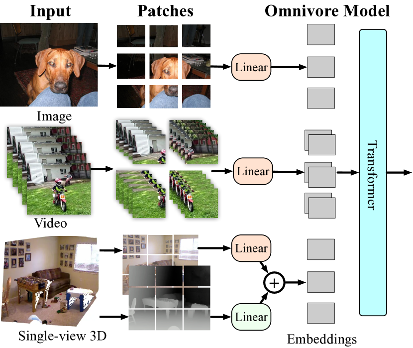
Figure 2: Multiple visual modalities in the Omnivore model. We convert image, video, and single-view 3D modalities into embeddings that are fed into a Transformer model. The images are converted into patches, videos into spatio-temporal tubes, and the single-view 3D images are converted into RGB patches and depth patches. The patches are projected into embeddings using linear layers. We use the same linear layer for (image or video) RGB patches and a separate one for depth patches.

2 Related Work

We build on prior work in ConvNet architectures, Transformers, multi-modal learning, and multi-task learning.

ConvNet architectures in vision. ConvNet architectures [48, 26] have been popular for many computer vision tasks in images, video, and 3D recognition. 2D convolutions are the main building block in ConvNets for images [46, 84, 77, 34], whereas 3D convolutions are used on 3D data [32, 18] or are combined with 2D convolutions for recognition of videos [90, 91, 13]. I3D [13] introduced a way to “inflate” 2D image convolutions into 3D convolutions, which allows 3D ConvNets for videos and 3D data to leverage image data indirectly via initialization from pretrained image models. Since video and 3D datasets are relatively small, they benefit from inflated pretrained image networks. However, while the inflation technique is applicable only to model finetuning, Omnivore models are pretrained jointly on images, videos, and single-view 3D data.

Transformers in vision. The Transformer architecture [92] originally proposed for NLP tasks has been successfully applied in computer vision on images [93, 94, 11, 21, 88, 70], video [5, 8, 52, 28, 66, 29], and 3D data [68, 103, 60]. Models such as ViT [21], Swin [51], and MViT [24] perform competitively on benchmark tasks such as image classification, detection, and video recognition. For example, Swin [51, 52] and MViT [24] require minimal changes to be used in image or video recognition tasks. Similarly, the Perceiver [38] can model image, point cloud, audio, and video inputs. However, all these studies train separate models for each visual modality. Instead, we train a single model on multiple input modalities simultaneously, which equips our model with cross-modal generalization capabilities.

Multi-modal learning. Our work uses multiple visual modalities to train the model. Multi-modal learning architectures may involve training separate encoders for each type of input modality. For example, a range of tasks require training separate encoders for images and text [59, 30, 41, 57, 15], for video and audio [63, 62, 3, 4, 67, 71], or for video and optical flow [77]. Recently, Transformers have been used to fuse multiple modalities: Transformers have been used to fuse features in vision-and-language tasks [40, 49, 37, 17, 56, 86, 83, 2] and video-and-audio tasks [64], video-and-image tasks [7], and even tasks that involve video, audio, and text [1]. Unlike our work, most prior work assumes that all input modalities are in correspondence and available simultaneously, which restricts them to using only multi-modal datasets. In our work, we train a single model on different visual modalities without assuming simultaneous access to all modalities. This allows us to leverage standard off-the-shelf single-modality vision datasets and we show that using a single shared encoder naturally leads to cross-modal generalization.

Multi-task learning. Our work is also related to studies on multi-task learning [14], which develop models that output predictions for multiple tasks on the same input [23, 44, 58, 102, 61, 27]. Such multi-task learners are known to work well when the target tasks exhibit strong similarities [99, 61]. They differ from Omnivore in that they operate on a single input modality but are trained to perform multiple tasks. By contrast, our models are trained to perform a single task (i.e., classification) on a variety of input modalities. Other multi-task learners operate on multi-modal inputs [39], but they use hand-designed model components for each modality.

3 Approach

Our goal is to learn a single model that can operate on three major visual modalities: images, videos, and single-view 3D. Because the model’s input modalities have different sizes and layouts—videos have a temporal axis and single-view 3D has an extra depth channel—this poses a challenge in designing the model. To overcome this challenge, we adopt the Transformer [92] architecture because the self-attention mechanism gracefully handles variable-sized inputs. Fig. 2 presents an overview of our approach.

3.1 The Omnivore Model

We convert all visual modalities into a common format by representing them via embeddings. Our model then uses a series of spatio-temporal attention operations to construct a unified representation of the different visual modalities.

Input patches. We represent the different types of visual input as a 4D tensor $\mathbf{X}\in\mathbb{R}^{T\times H\times W\times C}$, where $T$ is the size of the temporal dimension, $H$ and $W$ of the spatial dimensions, and $C$ of the channel dimension. Thus, RGB images $\mathbf{I}\in\mathbb{R}^{1\times H\times W\times 3}$ have $T\!=\!1$ frame with $C\!=\!3$ channels, RGB videos $\mathbf{V}\in\mathbb{R}^{T\times H\times W\times 3}$ have $T\!>\!1$ frames, and single-view 3D images $\mathbf{D}\in\mathbb{R}^{1\times H\times W\times 4}$ have $T\!=\!1$ frame with three RGB channels and one depth channel.

We follow [51, 21, 52] and split the input into a collection of patches. We illustrate this process in Fig. 2. Specifically, we convert the visual input $\mathbf{X}$ into a set of 4D sub-tensors $\mathbf{x}$ of size $t\times{h}\times{w}\times c$. Images $\mathbf{I}$ are split into a set of non-overlapping image patches of size $1\times{h}\times{w}\times 3$. Similarly, videos $\mathbf{V}$ are split into a set of non-overlapping spatio-temporal patches of shape $t\times{h}\times{w}\times 3$. For single-view 3D images $\mathbf{D}$, the image (RGB) and depth (D) channels are converted separately into patches of size $1\times{h}\times{w}\times 3$ and $1\times{h}\times{w}\times 1$, respectively.

Model architecture. Our model $f$ maps the resulting spatio-temporal visual patches into a shared representation $\mathbf{\Phi}$ for images, videos, and single-view 3D. We design the model to enable maximal parameter sharing across visual modalities. The input layer of the model processes each patch $\mathbf{x}$ independently, and projects the patches into an embedding $\mathbf{e}$ using a linear layer followed by a LayerNorm [6] (linear+LN). Each patch $\mathbf{x}$ of shape $t\times{h}\times{w}\times c$ is converted into an embedding of size $d$. We use the same layers to embed all the three-channel RGB patches, i.e., for image patches, video patches, and patches of the first three channels of a single-view 3D image. We zero-pad the single-frame patches on one side to ensure all patches have the same shape, $t\times{h}\times{w}\times 3$. We use a separate linear+LN layer to embed the depth-channel patches and add its output to the embedding of the corresponding RGB patch.

We use the same model (parameters) to process all the resulting embeddings. While Omnivore can use any vision transformer architecture [24, 21] to process the patch embeddings, we use the Swin transformer architecture [51] as our base model given its strong performance on image and video tasks. We rely on the self-attention [92] operation for spatio-temporal modeling across the patch embeddings, $\mathbf{e}$. Akin to [51], the self-attention involves patch embeddings from spatially and temporally nearby patches. We also use two sets of relative positional encodings: one for the spatial dimension and the other for the temporal dimension.

3.2 Training the Omnivore Model

The Omnivore model $f$ creates a single embedding $f(\mathbf{X})=\mathbf{\Phi}$ for multiple types of visual inputs. We train our model using a collection of classification tasks that provide inputs $\{(\mathbf{X}_{i},y_{i})\}$ with a visual input, $\mathbf{X}_{i}$, and a label, $y_{i}$. For example, we train most Omnivore models jointly on the ImageNet-1K dataset for image classification, the Kinetics-400 dataset for action recognition, and the SUN RGB-D dataset for single-view 3D scene classification.

This approach is similar to multi-task learning [14] and cross-modal alignment [15], but there important differences. In particular, we neither assume that the input observations are aligned (i.e., we do not assume access to correspondences between images, videos, and 3D data) nor do we assume that these datasets share the same label space. To achieve this, we employ dataset-specific linear classification layers on top of the final representation, $\mathbf{\Phi}$, produced by the model. The training loss of a sample is computed based solely on the output of the classification layer that corresponds to that sample’s source dataset.

Loss and optimization. We train Omnivore to minimize the cross-entropy loss on the training datasets using mini-batch SGD. We experiment with two different mini-batch construction strategies for SGD. In our first strategy, we construct mini-batches from each dataset (modality) separately. This strategy is easy to implement but alternating between datasets may potentially lead to training instabilities. Hence, we experiment with a second strategy that constructs mini-batches that mix samples from all datasets. We evaluate both mini-batch construction strategies in § 4.3.

4 Experiments

We perform a series of experiments to assess the effectiveness of Omnivore. Specifically, we compare Omnivore models to their modality-specific counterparts and to state-of-the-art models on a variety of recognition tasks. We also ablate several design choices we made in Omnivore.

Pre-training datasets. We train Omnivore on images from the ImageNet-1K dataset [75], videos from the Kinetics dataset [42], and single-view 3D images from the SUN RGB-D dataset [79]. We measure the top-1 and top-5 classification accuracy of our models on the respective validation sets. We note that the three datasets have negligible overlap in their visual concepts: ImageNet-1K focuses on object-centric classes, Kinetics-400 on action classes, and SUN RGB-D on indoor scene classes.

Images. The ImageNet-1K (IN1K) dataset has $\scriptstyle\sim$1.2M training and 50K validation images that comprise 1,000 classes.

Videos. The Kinetics-400 (K400) dataset consists of $\scriptstyle\sim$240K training and 20K validation video clips that are 10 seconds long, and are labeled into one of 400 action classes.

Single-view 3D. The SUN RGB-D dataset has $\scriptstyle\sim$5K train and $\scriptstyle\sim$5K val RGBD images with 19 scene classes. Following [74], we convert the depth maps into disparity maps.

Implementation details. We use the Swin transformer [51, 52] architecture as the backbone for Omnivore, and attach linear heads for each target dataset. At training time, we use a resolution of $224\!\times\!224$ and train using standard image augmentations [88] on ImageNet. For Kinetics, we sample 32 frames at stride 2. SUN RGB-D is processed similarly to ImageNet but we randomly drop the RGB channels with a probability of $0.5$ in order to encourage the model to use the depth channel for recognition as well. We provide complete implementation details in Appendix A. Our models are optimized using AdamW [53] for 500 epochs where a single epoch consists of one epoch each for ImageNet-1K and Kinetics, and 10 epochs for SUN RGB-D.

Transfer datasets and metrics. We evaluate Omnivore in transfer learning experiments on a diverse set of image, video, and single-view 3D tasks; see Table 1 for a summary. We present details on the experimental setup in Appendix B.

Dataset	Task	#cls	#train	#val
iNaturalist-2018 (iNat18) [36]	Fine-grained cls.	8142	437K	24K
Oxford-IIIT Pets (Pets) [69]	Fine-grained cls.	37	3.6K	3.6K
Places-365 (P365) [105]	Scene cls.	365	1.8M	36K
Something Something-v2 (SSv2) [31]	Action cls.	174	169K	25K
EPIC-Kitchens-100 (EK100) [20]	Action cls.	3806	67K	10K
NYU-v2 (NYU) [65]	Scene cls.	10	794	653
NYU-v2-seg (NYU-seg) [65]	Segmentation	40	794	653

Table 1: Transfer datasets used to evaluate Omnivore on image, video and single-view 3D modalities. The table reports the task, number of classes (#cls), number of training samples (#train), and number of validation samples (#val) for each dataset.

Images. We evaluate Omnivore on fine-grained object recognition on the iNaturalist-2018 dataset [36], fine-grained classification on the Oxford-IIIT Pets dataset [69], and in scene classification on the Places-365 dataset [105].

Videos. We use the Something Something-v2 dataset, which has a special emphasis on temporal modeling for action recognition. We also use the EPIC-Kitchens-100 dataset, which has 100 hours of unscripted egocentric video. Each clip is labeled with a verb and a noun that together form an action. Our model is trained to recognize all 3,806 actions, i.e., verb-noun pairs in the dataset. We marginalize over verbs to obtain noun predictions and vice versa.

Single-view 3D. We use the NYU-v2 dataset for single-view 3D scene classification and segmentation. We follow the setup from [33] for scene classification and [33, 10] for segmentation. For segmentation, we follow [51] and use the UPerNet [95] head with the Swin trunk.

4.1 Comparison with Modality-Specific Models

	ImageNet-1K		Kinetics-400		SUN
Method	top-1	top-5	top-1	top-5	top-1
ImageSwin-T [51]	81.2	95.5	✗	✗	✗
VideoSwin-T [52]	✗	✗	78.8	93.6	✗
DepthSwin-T	✗	✗	✗	✗	63.1
Omnivore (Swin-T)	80.9	95.5	78.9	93.8	62.3
ImageSwin-S [51]	83.2	96.2	✗	✗	✗
VideoSwin-S [52]	✗	✗	80.6	94.5	✗
DepthSwin-S	✗	✗	✗	✗	64.9
Omnivore (Swin-S)	83.4	96.6	82.2	95.4	64.6
ImageSwin-B [51]	83.5	96.5	✗	✗	✗
VideoSwin-B [52]	✗	✗	80.6	94.6	✗
DepthSwin-B	✗	✗	✗	✗	64.8
Omnivore (Swin-B)	84.0	96.8	83.3	95.8	65.4

Table 2: Omnivore vs. modality-specific models that have the same model architecture and number of parameters. Omnivore is a single model trained from scratch jointly on the IN1K, K400 and SUN datasets whereas the modality-specific models are trained specifically for each dataset (modality). The ImageSwin model is trained from scratch while the VideoSwin and DepthSwin models are finetuned from the ImageSwin model. Omnivore performs at-par or outperforms modality-specific models.

Figure 3: Comparing Omnivore with VideoSwin on K400. Omnivore improves over VideoSwin on F1 score on all 38 class groups defined in [42] (top 15 shown here for brevity).

		P365		iNat18		Pets		SSv2		EK100		NYU	NYU-seg
Model	Method	top-1	top-5	top-1	top-5	top-1	top-5	top-1	top-5	top-1	top-5	top-1	mIoU
Swin-T	Specific	57.9	87.3	69.7	87.6	93.7	99.6	62.2	88.7	41.8	62.8	72.5	47.9
	Omnivore	58.2	87.4	69.0	87.7	94.2	99.7	64.4	89.7	42.7	63.1	77.3	49.7
Swin-S	Specific	58.7	88.1	72.9	90.2	94.4	99.6	66.8	91.1	42.5	63.4	76.7	51.3
	Omnivore	58.8	88.0	73.6	90.8	95.2	99.7	68.2	91.8	44.9	64.8	76.9	52.7
Swin-B	Specific	58.9	88.3	73.2	90.9	94.2	99.7	65.8	90.6	42.8	64.0	76.4	51.1
	Omnivore	59.2	88.3	74.4	91.1	95.1	99.8	68.3	92.1	47.4	67.7	79.4	54.0

Table 3: Comparing Omnivore with modality-specific models after finetuning the models on seven downstream tasks. Results are presented for three different model sizes: T, S, and B. Our image specific model is pretrained on IN1K. The video specific and single-view 3D specific models are both initialized using inflation from the pretrained image-specific model and finetuned on K400 and SUN RGB-D respectively. Omnivore models are at par with or outperform modality-specific models on nearly all downstream tasks.

We compare Omnivore to models trained on a specific visual modality. We train Omnivore from scratch jointly on the IN1K, K400, and SUN datasets. Our modality-specific baseline models use the same Swin transformer architecture as Omnivore; we refer to them as ImageSwin, VideoSwin, and DepthSwin. Excluding the patch-embedding linear layers, these models have the same number of parameters as Omnivore. Following standard practice [52, 51], the ImageSwin model is trained on IN1K, whereas VideoSwin and DepthSwin models are finetuned by inflating the ImageSwin model. We experiment with three model sizes: viz., Swin-T, Swin-S, and Swin-B.

Pretraining performance. In Table 2, we compare Omnivore to modality-specific models on the pretraining datasets. The results in the table show that across model sizes, Omnivore models match or exceed the performance of their modality-specific counterparts. This observation supports our hypothesis that it is possible to learn a single visual representation that works across visual modalities. Omnivore learns representations that are as good as modality-specific representations using the same training data, same model parameters and same model capacity. This implies that Omnivore provides a viable alternative to the pretrain-then-finetune paradigm commonly used to deploy modality-specific models: it can deliver the same or better recognition accuracy with a third of the parameters.

From our results, we also observe that higher-capacity models benefit more from omnivorous training. Omnivore models using the larger Swin-B architecture improve over their modality-specific counterparts on both IN1K and K400, whereas the smallest Swin-T model does not.

Fig. 3 presents a detailed analysis of the improvements of Omnivore over the VideoSwin baseline (both using the Swin-B architecture) on the K400 dataset. Here VideoSwin is pre-trained on IN1K and finetuned on K400, whereas Omnivore is trained jointly on IN1K, K400, and SUN RGB-D. Both models use the the Swin-B architecture. Omnivore particularly improves the recognition of classes that require reasoning about parts of the human body such as the hands, arms, head, mouth, hair etc. We surmise this is because joint training on images helps Omnivore to learn a better model of the spatial configuration of parts.

Transfer learning performance. We compare Omnivore to modality-specific models by finetuning on various downstream tasks. Table 3 presents the results of these experiments. We observe that Omnivore transfers better than modality-specific models on nearly all downstream tasks. In particular, Omnivore provides significant gains on video-recognition tasks, even though it does not get any additional video supervision during pre-training compared to the baseline. We reiterate that Omnivore has the same model capacity as the modality-specific baselines. This observation underscores one of the key benefits of multi-modal training: because Omnivore was pretrained jointly on more diverse training data, it generalizes better out-of-distribution. As before, Table 3 also shows that higher-capacity models benefit the most from omnivorous training.

	ImageNet-1K		Kinetics-400		SUN
Method	top-1	top-5	top-1	top-5	top-1
MViT-B-24 [24]	83.1	-	✗	✗	✗
ViT-L/16 [21]	85.3	-	✗	✗	✗
ImageSwin-B [51]	85.2	97.5	✗	✗	✗
ImageSwin-L [51]	86.3	97.9	✗	✗	✗
ViT-B-VTN [66]	✗	✗	79.8	94.2	✗
TimeSformer-L [8]	✗	✗	80.7	94.7	✗
ViViT-L/16x2 320 [5]	✗	✗	81.3	94.7	✗
MViT-B 64$\times$3  [24]	✗	✗	81.2	95.1	✗
VideoSwin-B [52]	✗	✗	82.7	95.5	✗
VideoSwin-L [52]	✗	✗	83.1	95.9	✗
DF2Net [50]	✗	✗	✗	✗	54.6
G-L-SOOR [80]	✗	✗	✗	✗	55.5
TRecgNet [22]	✗	✗	✗	✗	56.7
CNN-RNN [9]	✗	✗	✗	✗	60.7
Depth Swin-B	✗	✗	✗	✗	69.1
Depth Swin-L	✗	✗	✗	✗	68.7
Omnivore (Swin-B)	85.3	97.5	84.0	96.2	67.2
Omnivore (Swin-L)	86.0	97.7	84.1	96.3	67.1

Table 4: Comparing Omnivore with state-of-the-art models on the image, video, and single-view 3D classification datasets used to pre-train Omnivore. Omnivore performs on par with or better than state-of-the-art models on all three pre-training tasks, including modality-specific models of similar size.

4.2 Comparison with the state-of-the-art

Next, we perform experiments comparing Omnivore to existing state-of-the-art models. In these experiments, like many state-of-the-art modality-specific methods, we use the ImageNet-21K (IN21K) dataset during pretraining. The Omnivore Swin-B and Swin-L models are trained from scratch on IN21K, IN1K, K400, and SUN, where a single epoch consists of one epoch each of IN1K and K400, 10 epochs of SUN, and 0.1 epochs of ImageNet-21K. Table 4 compares the performance of the Omnivore models to state-of-the-art models on each of the three benchmarks. Omnivore performs at par with or exceeds modality-specific methods despite using a model architecture that is not tailored towards any specific modality. Even when compared to modality-specific models with a similar number of parameters, Omnivore models match the state-of-the-art on IN1K, and outperform the previous state-of-the-art on K400 by achieving 84.1% accuracy – a gain of 1% which was previously only possible by using additional large video datasets. This demonstrates the strong performance of using the same Omnivore model across image, video and single-view 3D benchmarks.

Method	P365	iNat18	Pets
EfficientNet B6 [96, 78]	58.5	79.1	95.4
EfficientNet B7 [96, 78]	58.7	80.6	–
EfficientNet B8 [96, 78]	58.6	81.3	–
DeiT-B [88] $\uparrow$	–	79.5	–
ViT-B/16 [21, 78] $\uparrow$	58.2	79.8	–
ViT-L/16 [21, 78] $\uparrow$	59.0	81.7	–
Omnivore (Swin-B)	59.3	76.3	95.5
Omnivore (Swin-B $\uparrow$)	59.6	82.6	95.9
Omnivore (Swin-L)	59.4	78.0	95.7
Omnivore (Swin-L $\uparrow$)	59.9	84.1	96.1

Table 5: Comparing Omnivore with state-of-the-art models in image classification finetuning experiments on three datasets. Omnivore representations generalize well to scene classification (P365) and fine-grained classification (iNat18, Pets). $\uparrow$ indicates finetuning on a higher resolution image ($384\!\times\!384$px; see [89]).

Transfer learning performance. We compare Omnivore models to modality-specific models by finetuning on downstream tasks. In Table 5, we report results on image classification. Omnivore models outperform prior state-of-the-art in scene classification on Places-365, and in fine-grained classification on iNaturalist-2018 and Oxford-IIIT Pets.

We finetune Omnivore on video-classification and report the results in Table 6. On the EPIC-Kitchens-100 dataset, the Omnivore Swin-B model achieves the absolute best performance across verb, noun, and verb-noun pair (action) classification. Similarly, on the SSv2 dataset, which requires temporal reasoning, Omnivore outperforms all prior work. This suggests that Omnivore representations transfer well to temporal-reasoning tasks – Omnivore sets a new state-of-the-art while outperforming architectures specialized for these video tasks.

Finally, in Table 7, we report finetuning results for RGBD scene classification and segmentation. While prior work relies on specialized 3D operators [10], fusion techniques [97], or depth encoding schemes [33], Omnivore uses a generic architecture and operates directly on disparity. Omnivore achieves state-of-the-art performance on both the scene classification and segmentation tasks.

4.3 Ablation Study

	EK100			SSv2
Method	verb	noun	action	top-1	top-5
RGB-only methods
SlowFast [25]	65.6	50.0	38.5	63.0	88.5
TimeSformer [8]	–	–	–	62.4	–
MViT-B-24 [24]	–	–	–	68.7	91.5
TAR [76]	66.0	53.4	45.3	–	–
VIMPAC [87]	–	–	–	68.1	–
ViViT-L [5]	66.4	56.8	44.0	65.9	89.9
MFormer-L [72]	67.1	57.6	44.1	68.1	91.2
ORViT [35]	68.4	58.7	45.7	69.5	91.5
CoVeR [100]	–	–	–	70.9	–
VideoSwin-B [52]	67.8	57.0	46.1	69.6	92.7
Omnivore (Swin-B)	69.5	61.7	49.9	71.4	93.5
Multi-modal methods
MML [45]	–	–	–	69.1	92.1
MTCN [43]	70.7	62.1	49.6	–	–

Table 6: Comparing Omnivore with state-of-the-art models in video classification finetuning experiments on two datasets. We highlighted columns that show the two primary classification metrics used in prior work. Omnivore models obtain state-of-the-art results on both datasets, even outperforming some multi-modal methods.

Method		Classification	Segmentation
DF2Net [50]		65.4	✗
TRecgNet [22]		69.2	✗
ShapeConv [10]		✗	51.3
BCMFP + SA-Gate [16]		✗	52.4
TCD [97]		✗	53.1
Omnivore (Swin-B)		80.0	55.1
Omnivore (Swin-L)		80.3	56.8

Table 7: Comparing Omnivore with state-of-the-art models in RGBD finetuning experiments on the NYU-v2 dataset. The left column shows the scene classification accuracy while the right column shows the mean intersection-over-union of semantic segmentation. Omnivore outperforms prior art in RGBD classification and segmentation.

We ablate some of Omnivore’s key design choices in Table 8. Together, the results suggest Omnivore’s performance is relatively stable under different design choices. For a faster turnaround time in the ablations, we train the model for 300 epochs.

Training from scratch or finetuning. We compare training Omnivore models from scratch on different modalities (top row) with initializing the model via image classification followed by finetuning on all modalities (second row). For the finetuning result, we initialize Omnivore (Swin-B) using a pretrained ImageNet-21K model followed by joint finetuning on IN1K, K400, and SUN for 100 epochs. The model trained from scratch performs better in both image and video classification.

Data ratio. Since the IN1K and K400 datasets are much larger than SUN, we replicate SUN when training Omnivore. Although replication helps, a higher replication factor hurts the model performance on SUN (which hints at overfitting), whereas the performance on IN1K and K400 is unchanged. Based on the same logic, we undersample the IN21K dataset to have a similar size as IN1K. Increasing the proportion of IN21K has no effect on IN1K, decreases performance on K400, and improves performance on SUN. Hence, we use the 0.1:1:1:10 setting for our final model.

Batching strategy. We evaluate the two different batching strategies described in § 3, and observe that they perform similarly. We also find that the separate batching strategy (which alternates between datasets during training) does not lead to instabilities during training. Additionally, since it is easier to implement, we use it to train Omnivore.

Patch embedding model for depth channel. Omnivore uses a separate linear+LN layer for the depth channel in RGBD images. We compare this to using a four-channel convolutional model to embed depth patches instead, and find that the separate layer leads to better performance on SUN. We also observed that using the separate layer helps Omnivore transfer better to downstream RGBD tasks.

		IN1K	K400	SUN
Baseline		85.2	83.2	65.5
Finetuned		–0.7	–0.9	+0.9
Data ratio	0.1:1:1:1	–0.1	+0.3	–0.7
IN21K:IN1K:K400:SUN	0.1:1:1:10	+0	+0.1	+0.6
	0.1:1:1:20	+0	+0.2	+0.6
	0.1:1:1:100	–0.1	–0.1	–2.1
	0.3:1:1:50	+0.1	–1.3	+1.5
	0.6:1:1:50	–0.2	–3.1	+1.0
	1.0:1:1:50	–0.1	–4.5	+2.0
Batching	Mixed	–0.2	–0.1	–0.4
Patch embedding	RGBD Conv.	–0.1	+0.1	–2.2

Table 8: Ablation study of design choices made when training Omnivore. Our baseline settings use a data ratio of 0.1:1:1:50, the separate batching strategy, linear layers for embedding RGB and depth channels, and 300 epoch training. Omnivore’s performance is robust under different decisions. Omnivore trained from scratch (top row) performs slightly better than a jointly finetuned model (second row).

5 Cross-Modal Generalization

A key advantage of Omnivore over modality-specific models is that it can generalize across visual modalities. This generalization emerges naturally because we use the same model for all modalities. Our model is neither trained with corresponding data across modalities nor with any cross-modal consistency losses.

Query	Retrieved depth maps $\xrightarrow{\hskip 56.9055pt}$

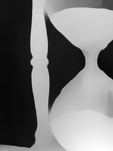
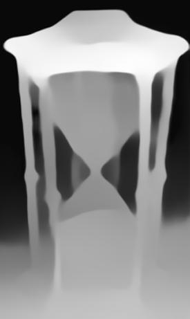
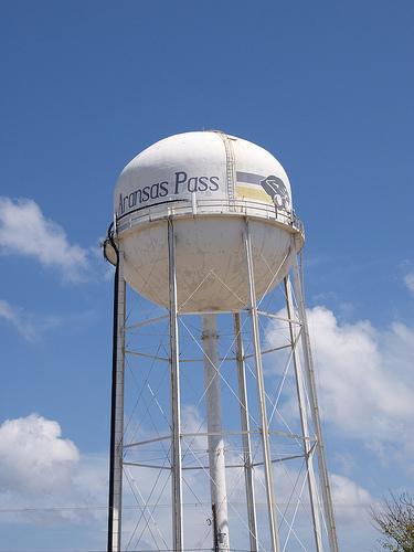
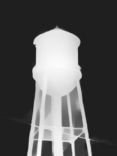
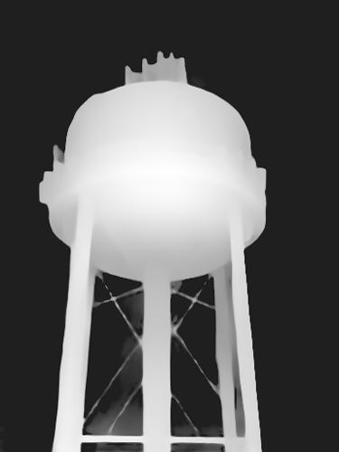
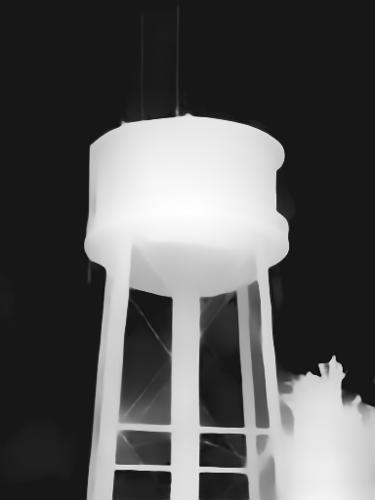
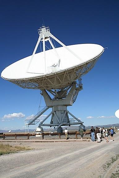
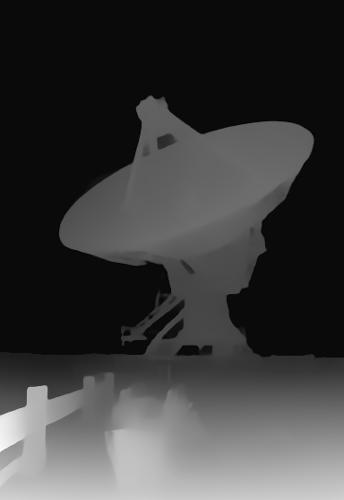
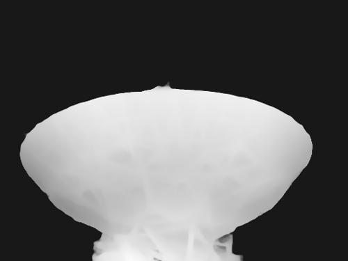
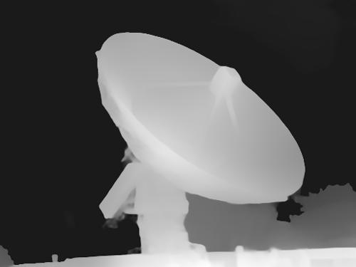
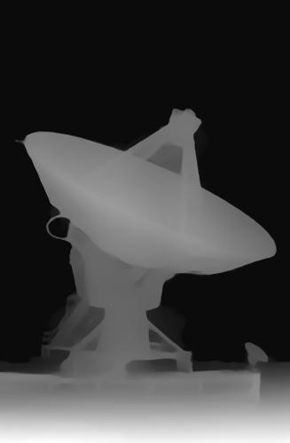
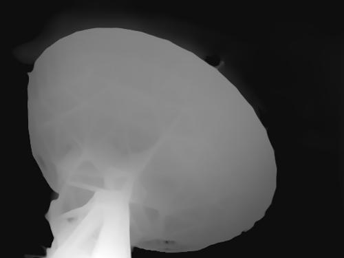
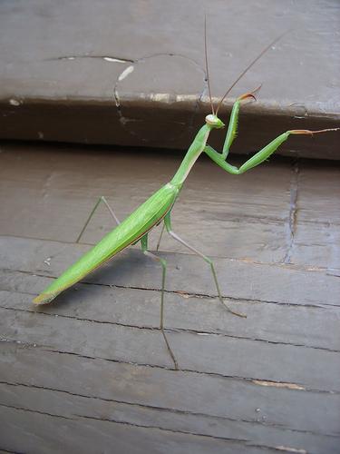
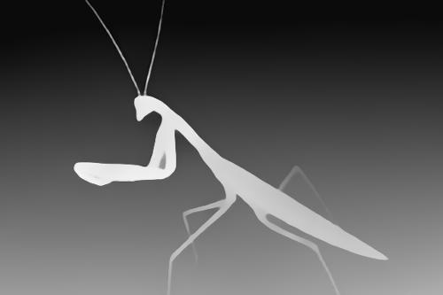
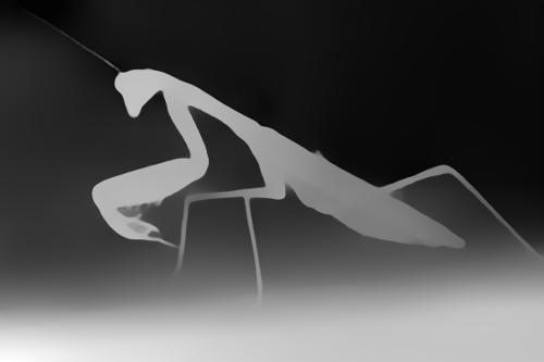
Figure 4: Retrieving depth maps given RGB images on the ImageNet-1K dataset. We show retrieved depth maps from the IN1K training set (right) for RGB image queries from the IN1K validation set (left). Although Omnivore was not trained on IN1K depth maps, the shared visual representation enables it to retrieve depth maps that are semantically similar to the query.

Retrieval across images and depth. We use the Omnivore representation to retrieve depth maps given an RGB image. To create a database of depth maps, we run a monocular depth-prediction model [74] on the ImageNet-1K train set. We note that Omnivore was not trained on ImageNet-1K depth maps nor on predicted depth. We use the ImageNet-1K val set (RGB) images as queries. Fig. 4 shows five examples of retrieved maps. These results illustrate that Omnivore constructs good depth-map representations, even though it had not previously observed ImageNet-1K depth maps during training. We emphasize that this cross-modal generalization ability is not the result of explicitly learning correspondences between visual modalities [33, 77]. Instead, it emerges due to the use of an almost entirely shared encoder for those modalities.

Classifying based on different modalities.

Method	RGB	D	RGBD
Omnivore (Swin-B)	84.3	63.1	83.7

To quantitatively measure Omnivore’s generalization performance across different modalities, we perform $k$-nearest neighbor ($k$-NN, $k\!=\!20$) classification experiments on the ImageNet-1K dataset using the predicted depth maps. We extract Omnivore representations from the RGB images on the val set and measure the model’s ability to retrieve images, RGBD images, and depth-only images from the train set. We observe that Omnivore produces a representation that allows for successful $k$-NN classification, which demonstrates its strong generalization performance. Surprisingly, we observe a high accuracy is attained even when retrieving depth-images, which provide less information about the object class than RGB images.

Retrieval across all modalities. We further probe the Omnivore visual representations in retrieval experiments across images, videos, and depth maps. We use the RGB images from the ImageNet-1K val set as queries and use them to retrieve similar depth maps from ImageNet-1K (predicted depth) and videos from Kinetics-400. Fig. 1 shows examples of the resulting retrievals. The results illustrate how Omnivore supports retrieval of visual concepts across images (RGB), single-view 3D (RGBD), and videos (RGBT) using its shared representation space.

Bridging frame-based and clip-based video models. Omnivore’s cross-modality generalization capabilities also make it more robust to changes in lengths of videos to be classified. We demonstrate this in in Fig. 5, where we classify videos using different length clips at inference time. The model is trained with 32 frames at stride 2, and by default uses 4 clips of the same length and stride to cover the full 10 second video at inference time. In this experiment, we vary the clip length from 1 to 32, increasing the number of clips proportionally to still cover the full video in each case. The results show that Omnivore’s performance degrades more gracefully as the video length decreases. Notably, Omnivore outperforms the baseline by 18.5% at a clip length of 1 frame (frame-level inference). This suggests that joint training on images and videos enables the model to use both temporal and spatial cues effectively.

Figure 5: Accuracy as a function of clip length on the K400 dataset. Models are trained on 32-frame clips but evaluated on clips of different length (with the same fps used for frame sampling). The performance of Omnivore degrades more gracefully than that of the VideoSwin-B model, and is still effective when doing frame-level inference (i.e., when the clip length is 1).

6 Discussion and Limitations

Although Omnivore presents an advance over traditional modality-specific models, it has several limitations. Current implementation of Omnivore only works on single-view 3D images and does not generalize to other 3D representations such as voxels, point clouds, etc. A simple approach to deal with such inputs may be to render multiple single-view 3D images from such inputs and average our predictions over those images, but such an approach would not effectively leverage multi-view information. Another caveat is that depth inputs are not scale-invariant; we used normalizations to alleviate this issue [74]. Also, Omnivore focuses only on visual modalities, so co-occurring modalities such as audio are not used. Omnivore was pretrained using only classification; using structured prediction tasks such as segmentation might yield richer representations. We leave such extensions to future work.

Ethical Considerations. Our study focuses on technical innovations in training models for visual recognition. These innovations themselves appear to be neutral from an ethics point-of-view. However, all ethical considerations that apply to other visual-recognition models apply equally to Omnivore. Any real-world deployment of a model like Omnivore is best preceded by a careful analysis of that model for ethical problems, including but not limited to: performance disparities between different user groups, associations that may be harmful to some users, and predictions that may propagate stereotypes.

Appendix A Implementation details for Pretraining

We train using AdamW with a batch size of 4096 for each dataset, and use a cosine learning rate (LR) schedule with linear warm up and cool down phases for the first and last 10% of training, respectively. We train for 500 epochs with a peak LR of $2\cdot{10}^{-3}$ and a weight decay of $5\cdot{10}^{-2}$. Swin-T, Swin-S and Swin-L use a window size of $8\!\times\!7\!\times\!7$, whereas Swin-B uses a window size of $16\!\times\!7\!\times\!7$. The models are trained with stochastic depth with a drop rate of $0.1$ for Swin-T, 0.2 for Swin-S, and 0.3 for Swin-B, and Swin-L. We use exponential moving average (EMA) [73] with a decay of $10^{-4}$ and report the best results during training since EMA results peak before the end of training.

For IN1K and IN21K we use RandAugment [19], mixup [101], CutMix [98], label smoothing [85], and Random Erasing [104] with the same settings as used in [88], and color jittering of 0.4. For SUN RGB-D we clamp and normalize the disparity channel, drop the RGB channels with a probability of 0.5, and we also apply 0.5 Dropout [82] before the linear head when pre-training with ImageNet-21K. For Kinetics-400 we use mixup, CutMix and label smoothing, and Dropout of $0.5$ before the linear head.

Appendix B Details on the Transfer Tasks

B.1 Image Classification

We finetune all models on the downstream tasks for 100 epochs and optimize the models with mini-batch SGD. We use a half-wave cosine learning rate [54] and set the weight decay to zero. For all models, including the modality-specific models, we perform a grid search for the best learning rate in the range [5e-3, 1e-2, 2e-2, 4e-2, 8e-2, 1e-1, 2e-1, 3e-1, 4e-1, 5e-1, 6e-1] and drop path in [0.1, 0.3]. We use the strong augmentations from [88] for finetuning. For the evaluations in Tables 3 and 5, we follow [78] and resize the images to shortest side of $224$px and evaluate the models on the center crop of $224\times 224$. For higher resolution ($384$px) evaluations in Table 5, we similarly resize the images to shortest side of $384$px and evaluate the models on the center crop of $384\times 384$. We also increase the spatial window size for all the Swin models from $7$ to $12$.

B.2 Video Classification

In Table 3, we finetune video models using hyperparameters as described in [52]. For Something Something-v2, we finetune for 60 epochs with AdamW optimizer. We use half-wave cosine learning rate with warmup. We start the learning rate from $10^{-6}$ and linearly warmup to a peak learning rate of $6\cdot\!10^{-3}$ over 5% of the training, and rest 95% we use half-wave cosine schedule to decay the learning rate back to $10^{-6}$. We train the classification head with this learning rate, and the backbone with $0.1\!\times$ the above learning rate. Throughout we use a weight decay of 0.05. We use a batch size of $4\!\times 64$ distributed over 64 32GB GPUs. For EPIC-Kitchens-100, we use similar hyperparamters with only difference being that we use a peak learning rate of $2\!\cdot\!10^{-3}$ and we train for 150 epochs. These settings provided better performance for the modality-specific baseline, and we use it for finetuning both the baseline and Omnivore models.

Figure 6: Gain of Omnivore over baseline on Action recognition (per group). We plot the gain in per-class F1-score on the K400 dataset for all the action groups defined in [13]. The baseline model is first pretrained on ImageNet-1K and then fine-tuned on K400 whereas Omnivore is trained jointly on ImageNet-1K, K400 and the single-view 3D SUN RGB-D dataset. Omnivore improves the performance for all the 38 groups.

Figure 7: Gain of Omnivore over baseline on Action Recognition (per class). We plot the gain in per-class F1-score on the K400 dataset for the top twenty and bottom twenty classes. The baseline model is first pretrained on ImageNet-1K and then fine-tuned on K400 whereas Omnivore is trained jointly on ImageNet-1K, K400 and the single-view 3D SUN RGB-D dataset. Omnivore improves the F1 score on 308 out of the 400 total classes.

In terms of preprocessing, at train time we sample a 32 frame video clip at stride 2 from the full video using temporal segment sampling as in [52]. We scale the short side of the video to 256px, take a 224px random resized crop, followed by RandAugment and Random Erasing. At test time, we again sample a 32 frame clip with stride 2, scale the short side to 224px and take 3 spatial crops along the longer axis to get $224\times 224$ crops. The final predictions are averaged over these crops.

For comparison to the state-of-the-art in Table 6, when finetuning Omnivore models trained with IN21K, we found slightly different hyperparameters to perform better. For Something Something-v2, we used peak learning rate of $1.2\cdot{10}^{-3}$ over 150 epochs. For EPIC-Kitchens-100, we used weight decay of 0.004, over 100 epochs, peak learning rate of $4\cdot{10}^{-4}$, with the same learning rate schedule for backbone and head. We also used cutmix augmentation and label smoothing. All other hyperparameters in both cases were as described earlier. We also use EMA with similar settings as used during pretraining.

B.3 Single-view 3D Tasks

NYU Scene classification. We follow the setup from [33] for scene classification and use 10 classes derived from the original 19 classes. In Table 7 (classification) the best Swin B and Swin L models were trained for 200 epochs with starting learning rate of $5\times 10^{-3}$, weight decay of 0 for Swin B and $1\times 10^{-4}$ for Swin L. All other hyperparameters were as described earlier.

NYU RGBD Segmentation. We follow the training and evaluation setup from [10]. We follow the Swin segmentation architecture which uses an UperNet [95] head with the Swin trunk. All models are finetuned with AdamW [53] with a weight decay of $0.01$. The learning rate follows a Polynomial Decay (power 1) schedule and starts at $0.00006$. We warmup the learning rate for 1500 iterations and train the model with a batchsize of 32. All the depth maps in NYU are converted into disparity maps by using the camera baseline and focal length of the Kinect sensor.

B.4 $k$-NN experiments

Extracting depth on ImageNet-1K.

We ran a monocular depth-prediction model [74] on the IN1K train set. We used the pretrained dpt_large model and followed the input image preprocessing steps as provided in [74].

Classifying ImageNet-1K using different modalities.

For the experiments involving classification using different modalities, we extract features from the IN1K train set using the RGB, RGBD or just Depth (D) modalities, and on IN1K validation set using the RGB modality. We follow the $k$-NN protocol from [12] for evaluation and briefly describe it next. We extract the stage 3 [51] features and $L_{2}$ normalize them. For each validation feature as the query, we retrieve the nearest neighbors from the train set using euclidean distance, and take the top-$k$ closest matches. For each match we create a one-hot vector using its ground truth label, and scale it by $e^{s/\tau}$, where $s$ is the dot product between the feature of the matched image the query image, and $\tau$ is a temperature hyperparameter (set to 0.07). We compute an effective prediction for the query by summing the top-$k$ one-hot vectors. Similar processing is used for the visualizations in Fig. 1 and Fig. 4.

Appendix C Other Results

Results on UCF-101. We also evaluate Omnivore on another popular (albeit smaller) video recognition benchmark, UCF-101 [81]. As shown in Table 9, Omnivore pre-training is effective for sports action recognition in UCF-101 as well. Note that the results shown are with RGB modality only; the state-of-the-art on these datasets often leverages additional features such as optical flow, dense trajectories (IDT) etc.

	VideoSwin-B	Omnivore (Swin-B)
3-split accuracy	96.9	98.2

Table 9: UCF-101. As in Table 3, the VideoSwin model is inflated from IN1K and pre-trained on K400. Omnivore is pre-trained with IN1K, K400 and SUN RGB-D. Both models are then finetuned and evaluated on UCF-101 for each split separately. Performance reported is averaged over the standard 3 splits.

Low-data regime fine-tuning. We analyzed low-shot versions of the Places-365 benchmark (models from Table 3). As shown in Table 10, Omnivore outperforms the modality-specific baseline in the low-shot regime too.

Method	Places-365
	1%	2%	5%	10%
Omnivore	46.2	49.0	51.5	53.9
Image-specific	44.8	47.9	50.9	53.4

Table 10: Low-shot finetuning. Performance of finetuning Omnivore on low-shot versions of the Places-365 dataset.

Per-class gains. We present the gain of Omnivore over the VideoSwin baseline (§ 4.1 of the main paper) in Figs. 6 and 7.

References

- [1] Hassan Akbari, Linagzhe Yuan, Rui Qian, Wei-Hong Chuang, Shih-Fu Chang, Yin Cui, and Boqing Gong. Vatt: Transformers for multimodal self-supervised learning from raw video, audio and text. arXiv preprint arXiv:2104.11178, 2021.
- [2] Jean-Baptiste Alayrac, Adria Recasens, Rosalia Schneider, Relja Arandjelovic, Jason Ramapuram, Jeffrey De Fauw, Lucas Smaira, Sander Dieleman, and Andrew Zisserman. Self-supervised multimodal versatile networks. NeurIPS, 2020.
- [3] Relja Arandjelovic and Andrew Zisserman. Look, listen and learn. In ICCV, 2017.
- [4] Relja Arandjelovic and Andrew Zisserman. Objects that sound. In ECCV, 2018.
- [5] Anurag Arnab, Mostafa Dehghani, Georg Heigold, Chen Sun, Mario Lucic, and Cordelia Schmid. ViViT: A video vision transformer. In ICCV, 2021.
- [6] Jimmy Lei Ba, Jamie Ryan Kiros, and Geoffrey E Hinton. Layer normalization. arXiv preprint arXiv:1607.06450, 2016.
- [7] Max Bain, Arsha Nagrani, Gül Varol, and Andrew Zisserman. Frozen in time: A joint video and image encoder for end-to-end retrieval. arXiv preprint arXiv:2104.00650, 2021.
- [8] Gedas Bertasius, Heng Wang, and Lorenzo Torresani. Is space-time attention all you need for video understanding? In ICML, 2021.
- [9] Ali Caglayan, Nevrez Imamoglu, Ahmet Burak Can, and Ryosuke Nakamura. When cnns meet random rnns: Towards multi-level analysis for rgb-d object and scene recognition. arXiv preprint arXiv:2004.12349, 2020.
- [10] Jinming Cao, Hanchao Leng, Dani Lischinski, Danny Cohen-Or, Changhe Tu, and Yangyan Li. Shapeconv: Shape-aware convolutional layer for indoor rgb-d semantic segmentation. In ICCV, 2021.
- [11] Nicolas Carion, Francisco Massa, Gabriel Synnaeve, Nicolas Usunier, Alexander Kirillov, and Sergey Zagoruyko. End-to-end object detection with transformers. In ECCV, 2020.
- [12] Mathilde Caron, Hugo Touvron, Ishan Misra, Hervé Jégou, Julien Mairal, Piotr Bojanowski, and Armand Joulin. Emerging properties in self-supervised vision transformers. In ICCV, 2021.
- [13] João Carreira and Andrew Zisserman. Quo vadis, action recognition? a new model and the kinetics dataset. In CVPR, 2017.
- [14] Rich Caruana. Multitask learning. Machine Learning, 1997.
- [15] Lluis Castrejon, Yusuf Aytar, Carl Vondrick, Hamed Pirsiavash, and Antonio Torralba. Learning aligned cross-modal representations from weakly aligned data. In CVPR, 2016.
- [16] Xiaokang Chen, Kwan-Yee Lin, Jingbo Wang, Wayne Wu, Chen Qian, Hongsheng Li, and Gang Zeng. Bi-directional cross-modality feature propagation with separation-and-aggregation gate for rgb-d semantic segmentation. In ECCV, 2020.
- [17] Yen-Chun Chen, Linjie Li, Licheng Yu, Ahmed El Kholy, Faisal Ahmed, Zhe Gan, Yu Cheng, and Jingjing Liu. Uniter: Universal image-text representation learning. In ECCV, 2020.
- [18] Christopher Choy, JunYoung Gwak, and Silvio Savarese. 4d spatio-temporal convnets: Minkowski convolutional neural networks. In CVPR, 2019.
- [19] Ekin D Cubuk, Barret Zoph, Jonathon Shlens, and Quoc V Le. Randaugment: Practical automated data augmentation with a reduced search space. In CVPR, 2020.
- [20] Dima Damen, Hazel Doughty, Giovanni Maria Farinella, Antonino Furnari, Evangelos Kazakos, Jian Ma, Davide Moltisanti, Jonathan Munro, Toby Perrett, Will Price, et al. Rescaling egocentric vision. IJCV, 2021.
- [21] Alexey Dosovitskiy, Lucas Beyer, Alexander Kolesnikov, Dirk Weissenborn, Xiaohua Zhai, Thomas Unterthiner, Mostafa Dehghani, Matthias Minderer, Georg Heigold, Sylvain Gelly, et al. An image is worth 16x16 words: Transformers for image recognition at scale. In ICLR, 2021.
- [22] Dapeng Du, Limin Wang, Huiling Wang, Kai Zhao, and Gangshan Wu. Translate-to-recognize networks for rgb-d scene recognition. In CVPR, 2019.
- [23] David Eigen and Rob Fergus. Predicting depth, surface normals and semantic labels with a common multi-scale convolutional architecture. In ICCV, 2015.
- [24] Haoqi Fan, Bo Xiong, Karttikeya Mangalam, Yanghao Li, Zhicheng Yan, Jitendra Malik, and Christoph Feichtenhofer. Multiscale vision transformers. In ICCV, 2021.
- [25] Christoph Feichtenhofer, Haoqi Fan, Jitendra Malik, and Kaiming He. Slowfast networks for video recognition. In ICCV, 2019.
- [26] Kunihiko Fukushima. A self-organizing neural network model for a mechanism of pattern recognition unaffected by shift in position. Biol. Cybern., 1980.
- [27] Golnaz Ghiasi, Barret Zoph, Ekin D Cubuk, Quoc V Le, and Tsung-Yi Lin. Multi-task self-training for learning general representations. In ICCV, 2021.
- [28] Rohit Girdhar, João Carreira, Carl Doersch, and Andrew Zisserman. Video action transformer network. In CVPR, 2019.
- [29] Rohit Girdhar and Kristen Grauman. Anticipative Video Transformer. In ICCV, 2021.
- [30] Yunchao Gong, Liwei Wang, Micah Hodosh, Julia Hockenmaier, and Svetlana Lazebnik. Improving image-sentence embeddings using large weakly annotated photo collections. In ECCV, 2014.
- [31] Raghav Goyal, Samira Ebrahimi Kahou, Vincent Michalski, Joanna Materzynska, Susanne Westphal, Heuna Kim, Valentin Haenel, Ingo Fruend, Peter Yianilos, Moritz Mueller-Freitag, Florian Hoppe, Christian Thurau, Ingo Bax, and Roland Memisevic. The “something something” video database for learning and evaluating visual common sense. In ICCV, 2017.
- [32] Benjamin Graham, Martin Engelcke, and Laurens van der Maaten. 3d semantic segmentation with submanifold sparse convolutional networks. In CVPR, 2018.
- [33] Saurabh Gupta, Pablo Arbelaez, and Jitendra Malik. Perceptual organization and recognition of indoor scenes from rgb-d images. In CVPR, 2013.
- [34] Kaiming He, Xiangyu Zhang, Shaoqing Ren, and Jian Sun. Deep residual learning for image recognition. In CVPR, 2016.
- [35] Roei Herzig, Elad Ben-Avraham, Karttikeya Mangalam, Amir Bar, Gal Chechik, Anna Rohrbach, Trevor Darrell, and Amir Globerson. Object-region video transformers. arXiv preprint arXiv:2110.06915, 2021.
- [36] Grant Van Horn, Oisin Mac Aodha, Yang Song, Yin Cui, Chen Sun, Alex Shepard, Hartwig Adam, Pietro Perona, and Serge Belongie. The inaturalist species classification and detection dataset. In CVPR, 2018.
- [37] Ronghang Hu and Amanpreet Singh. Unit: Multimodal multitask learning with a unified transformer. In ICCV, 2021.
- [38] Andrew Jaegle, Felix Gimeno, Andrew Brock, Andrew Zisserman, Oriol Vinyals, and Joao Carreira. Perceiver: General perception with iterative attention. ICML, 2021.
- [39] Lukasz Kaiser, Aidan N Gomez, Noam Shazeer, Ashish Vaswani, Niki Parmar, Llion Jones, and Jakob Uszkoreit. One model to learn them all. arXiv preprint arXiv:1706.05137, 2017.
- [40] Aishwarya Kamath, Mannat Singh, Yann LeCun, Gabriel Synnaeve, Ishan Misra, and Nicolas Carion. Mdetr-modulated detection for end-to-end multi-modal understanding. In ICCV, 2021.
- [41] Andrej Karpathy and Li Fei-Fei. Deep visual-semantic alignments for generating image descriptions. In CVPR, 2015.
- [42] Will Kay, Joao Carreira, Karen Simonyan, Brian Zhang, Chloe Hillier, Sudheendra Vijayanarasimhan, Fabio Viola, Tim Green, Trevor Back, Paul Natsev, et al. The kinetics human action video dataset. arXiv preprint arXiv:1705.06950, 2017.
- [43] Evangelos Kazakos, Jaesung Huh, Arsha Nagrani, Andrew Zisserman, and Dima Damen. With a little help from my temporal context: Multimodal egocentric action recognition. In BMVC, 2021.
- [44] Iasonas Kokkinos. UberNet: Training a universal convolutional neural network for low-, mid-, and high-level vision using diverse datasets and limited memory. In CVPR, 2017.
- [45] Stepan Komkov, Maksim Dzabraev, and Aleksandr Petiushko. Mutual modality learning for video action classification. arXiv preprint arXiv:2011.02543, 2020.
- [46] Alex Krizhevsky, Ilya Sutskever, and Geoffrey E Hinton. Imagenet classification with deep convolutional neural networks. NeurIPS, 2012.
- [47] Ivan Laptev and Tony Lindeberg. Space-time interest points. In ICCV, 2003.
- [48] Yann LeCun, Léon Bottou, Yoshua Bengio, and Patrick Haffner. Gradient-based learning applied to document recognition. Proceedings of the IEEE, 1998.
- [49] Xiujun Li, Xi Yin, Chunyuan Li, Pengchuan Zhang, Xiaowei Hu, Lei Zhang, Lijuan Wang, Houdong Hu, Li Dong, Furu Wei, Yejin Choi, and Jianfeng Gao. Oscar: Object-semantics aligned pre-training for vision-language tasks. In ECCV, 2020.
- [50] Yabei Li, Junge Zhang, Yanhua Cheng, Kaiqi Huang, and Tieniu Tan. Dfnet: Discriminative feature learning and fusion network for RGB-D indoor scene classification. In AAAI, 2018.
- [51] Ze Liu, Yutong Lin, Yue Cao, Han Hu, Yixuan Wei, Zheng Zhang, Stephen Lin, and Baining Guo. Swin transformer: Hierarchical vision transformer using shifted windows. In ICCV, 2021.
- [52] Ze Liu, Jia Ning, Yue Cao, Yixuan Wei, Zheng Zhang, Stephen Lin, and Han Hu. Video swin transformer. arXiv preprint arXiv:2106.13230, 2021.
- [53] Ilya Loshchilov and Frank Hutter. Decoupled weight decay regularization. arXiv preprint arXiv:1711.05101, 2017.
- [54] Ilya Loshchilov and Frank Hutter. Sgdr: Stochastic gradient descent with warm restarts. In ICLR, 2017.
- [55] David G Lowe. Distinctive image features from scale-invariant keypoints. IJCV, 2004.
- [56] Jiasen Lu, Dhruv Batra, Devi Parikh, and Stefan Lee. Vilbert: Pretraining task-agnostic visiolinguistic representations for vision-and-language tasks. arXiv preprint arXiv:1908.02265, 2019.
- [57] Jiasen Lu, Vedanuj Goswami, Marcus Rohrbach, Devi Parikh, and Stefan Lee. 12-in-1: Multi-task vision and language representation learning. In CVPR, 2020.
- [58] Kevis-Kokitsi Maninis, Ilija Radosavovic, and Iasonas Kokkinos. Attentive single-tasking of multiple tasks. In CVPR, 2019.
- [59] Antoine Miech, Jean-Baptiste Alayrac, Lucas Smaira, Ivan Laptev, Josef Sivic, and Andrew Zisserman. End-to-end learning of visual representations from uncurated instructional videos. In CVPR, 2020.
- [60] Ishan Misra, Rohit Girdhar, and Armand Joulin. An End-to-End Transformer Model for 3D Object Detection. In ICCV, 2021.
- [61] Ishan Misra, Abhinav Shrivastava, Abhinav Gupta, and Martial Hebert. Cross-stitch networks for multi-task learning. In CVPR, 2016.
- [62] Pedro Morgado, Ishan Misra, and Nuno Vasconcelos. Robust audio-visual instance discrimination. In CVPR, 2021.
- [63] Pedro Morgado, Nuno Vasconcelos, and Ishan Misra. Audio-visual instance discrimination with cross-modal agreement. In CVPR, 2021.
- [64] Arsha Nagrani, Shan Yang, Anurag Arnab, Aren Jansen, Cordelia Schmid, and Chen Sun. Attention bottlenecks for multimodal fusion. In NeurIPS, 2021.
- [65] Pushmeet Kohli Nathan Silberman, Derek Hoiem and Rob Fergus. Indoor segmentation and support inference from rgbd images. In ECCV, 2012.
- [66] Daniel Neimark, Omri Bar, Maya Zohar, and Dotan Asselmann. Video transformer network. arXiv preprint arXiv:2102.00719, 2021.
- [67] Andrew Owens and Alexei A Efros. Audio-visual scene analysis with self-supervised multisensory features. In ECCV, 2018.
- [68] Xuran Pan, Zhuofan Xia, Shiji Song, Li Erran Li, and Gao Huang. 3d object detection with pointformer. In CVPR, 2021.
- [69] Omkar M Parkhi, Andrea Vedaldi, Andrew Zisserman, and CV Jawahar. Cats and dogs. In CVPR, 2012.
- [70] Niki Parmar, Ashish Vaswani, Jakob Uszkoreit, Lukasz Kaiser, Noam Shazeer, Alexander Ku, and Dustin Tran. Image transformer. In ICML, 2018.
- [71] Mandela Patrick, Yuki M Asano, Ruth Fong, João F Henriques, Geoffrey Zweig, and Andrea Vedaldi. Multi-modal self-supervision from generalized data transformations. arXiv preprint arXiv:2003.04298, 2020.
- [72] Mandela Patrick, Dylan Campbell, Yuki M Asano, Ishan Misra Florian Metze, Christoph Feichtenhofer, Andrea Vedaldi, and João Henriques. Keeping your eye on the ball: Trajectory attention in video transformers. In NeurIPS, 2021.
- [73] Boris T Polyak and Anatoli B Juditsky. Acceleration of stochastic approximation by averaging. SIAM journal on control and optimization, 1992.
- [74] René Ranftl, Katrin Lasinger, David Hafner, Konrad Schindler, and Vladlen Koltun. Towards robust monocular depth estimation: Mixing datasets for zero-shot cross-dataset transfer. TPAMI, 2020.
- [75] Olga Russakovsky, Jia Deng, Hao Su, Jonathan Krause, Sanjeev Satheesh, Sean Ma, Zhiheng Huang, Andrej Karpathy, Aditya Khosla, Michael Bernstein, Alexander C. Berg, and Li Fei-Fei. ImageNet Large Scale Visual Recognition Challenge. IJCV, 2015.
- [76] Fadime Sener, Dibyadip Chatterjee, and Angela Yao. Technical report: Temporal aggregate representations. arXiv preprint arXiv:2106.03152, 2021.
- [77] Karen Simonyan and Andrew Zisserman. Two-stream convolutional networks for action recognition in videos. In NeurIPS, 2014.
- [78] Mannat Singh, Laura Gustafson, Aaron Adcock, Vinicius de Freitas Reis, Bugra Gedik, Raj Prateek Kosaraju, Dhruv Mahajan, Ross Girshick, Piotr Dollár, and Laurens van der Maaten. Revisiting weakly supervised pre-training of visual perception models. In CVPR, 2022.
- [79] Shuran Song, Samuel P Lichtenberg, and Jianxiong Xiao. Sun rgb-d: A rgb-d scene understanding benchmark suite. In CVPR, 2015.
- [80] Xinhang Song, Shuqiang Jiang, Bohan Wang, Chengpeng Chen, and Gongwei Chen. Image representations with spatial object-to-object relations for rgb-d scene recognition. TIP, 2020.
- [81] Khurram Soomro, Amir Roshan Zamir, and Mubarak Shah. UCF101: A dataset of 101 human action classes from videos in the wild. CRCV-TR-12-01, 2012.
- [82] Nitish Srivastava, Geoffrey Hinton, Alex Krizhevsky, Ilya Sutskever, and Ruslan Salakhutdinov. Dropout: a simple way to prevent neural networks from overfitting. JMLR, 2014.
- [83] Weijie Su, Xizhou Zhu, Yue Cao, Bin Li, Lewei Lu, Furu Wei, and Jifeng Dai. Vl-bert: Pre-training of generic visual-linguistic representations. arXiv preprint arXiv:1908.08530, 2019.
- [84] Christian Szegedy, Wei Liu, Yangqing Jia, Pierre Sermanet, Scott Reed, Dragomir Anguelov, Dumitru Erhan, Vincent Vanhoucke, and Andrew Rabinovich. Going deeper with convolutions. In CVPR, 2015.
- [85] Christian Szegedy, Vincent Vanhoucke, Sergey Ioffe, Jon Shlens, and Zbigniew Wojna. Rethinking the inception architecture for computer vision. In CVPR, 2016.
- [86] Hao Tan and Mohit Bansal. Lxmert: Learning cross-modality encoder representations from transformers. arXiv preprint arXiv:1908.07490, 2019.
- [87] Hao Tan, Jie Lei, Thomas Wolf, and Mohit Bansal. VIMPAC: Video pre-training via masked token prediction and contrastive learning. arXiv preprint arXiv:2106.11250, 2021.
- [88] Hugo Touvron, Matthieu Cord, Matthijs Douze, Francisco Massa, Alexandre Sablayrolles, and Hervé Jégou. Training data-efficient image transformers & distillation through attention. In ICML, 2021.
- [89] Hugo Touvron, Andrea Vedaldi, Matthijs Douze, and Hervé Jégou. Fixing the train-test resolution discrepancy. In NeurIPS, 2019.
- [90] Du Tran, Lubomir Bourdev, Rob Fergus, Lorenzo Torresani, and Manohar Paluri. Learning spatiotemporal features with 3d convolutional networks. In CVPR, 2015.
- [91] Du Tran, Heng Wang, Lorenzo Torresani, Jamie Ray, Yann LeCun, and Manohar Paluri. A closer look at spatiotemporal convolutions for action recognition. In CVPR, 2018.
- [92] Ashish Vaswani, Noam Shazeer, Niki Parmar, Jakob Uszkoreit, Llion Jones, Aidan N Gomez, Lukasz Kaiser, and Illia Polosukhin. Attention is all you need. In NeurIPS, 2017.
- [93] Wenhai Wang, Enze Xie, Xiang Li, Deng-Ping Fan, Kaitao Song, Ding Liang, Tong Lu, Ping Luo, and Ling Shao. Pyramid vision transformer: A versatile backbone for dense prediction without convolutions. In ICCV, 2021.
- [94] Xiaolong Wang, Ross Girshick, Abhinav Gupta, and Kaiming He. Non-local neural networks. In CVPR, 2018.
- [95] Tete Xiao, Yingcheng Liu, Bolei Zhou, Yuning Jiang, and Jian Sun. Unified perceptual parsing for scene understanding. In ECCV, 2018.
- [96] Cihang Xie, Mingxing Tan, Boqing Gong, Jiang Wang, Alan L Yuille, and Quoc V Le. Adversarial examples improve image recognition. In CVPR, 2020.
- [97] Yuchun Yue, Wujie Zhou, Jingsheng Lei, and Lu Yu. Two-stage cascaded decoder for semantic segmentation of rgb-d images. IEEE Signal Processing Letters, 2021.
- [98] Sangdoo Yun, Dongyoon Han, Seong Joon Oh, Sanghyuk Chun, Junsuk Choe, and Youngjoon Yoo. Cutmix: Regularization strategy to train strong classifiers with localizable features. In ICCV, 2019.
- [99] Amir Roshan Zamir, Alexander Sax, William B. Shen, Leonidas J. Guibas, Jitendra Malik, and Silvio Savarese. Taskonomy: Disentangling task transfer learning. In CVPR, 2018.
- [100] Bowen Zhang, Jiahui Yu, Christopher Fifty, Wei Han, Andrew M. Dai, Ruoming Pang, and Fei Sha. Co-training transformer with videos and images improves action recognition. arXiv preprint arXiv:2112.07175, 2021.
- [101] Hongyi Zhang, Moustapha Cisse, Yann N Dauphin, and David Lopez-Paz. mixup: Beyond empirical risk minimization. In ICLR, 2018.
- [102] Zhanpeng Zhang, Ping Luo, Chen Change Loy, and Xiaou Tang. Facial landmark detection by deep multi-task learning. In ECCV, 2014.
- [103] Hengshuang Zhao, Li Jiang, Jiaya Jia, Philip Torr, and Vladlen Koltun. Point transformer. In ICCV, 2021.
- [104] Zhun Zhong, Liang Zheng, Guoliang Kang, Shaozi Li, and Yi Yang. Random erasing data augmentation. In AAAI, 2020.
- [105] Bolei Zhou, Agata Lapedriza, Aditya Khosla, Aude Oliva, and Antonio Torralba. Places: A 10 million image database for scene recognition. TPAMI, 2017.