Abstract

A major objective of lattice QCD is the computation of hadronic matrix elements. The standard method is to use three-point and four-point correlation functions. An alternative approach, requiring only the computation of two-point correlation functions is to use the Feynman-Hellmann theorem. In this talk we develop this method up to second order in perturbation theory, in a context appropriate for lattice QCD. This encompasses the Compton Amplitude (which forms the basis for deep inelastic scattering) and hadron scattering. Some numerical results are presented showing results indicating what this approach might achieve.

1 Introduction

Understanding the internal structure of hadrons and in particular the nucleon directly from the underlying QCD theory is a major task of particle physics. It is complicated because of the non-perturbative nature of the problem, and presently the only known method is to discretise QCD and use numerical Monte Carlo methods. The relevant information is encoded in correlation functions – from the all encompassing two-quark correlation functions to GTMDs, TMDs, GPDs Wigner functions, PDFs and Form Factors, e.g. [1].

Using the Operator Product Expansion (OPE), it is possible to relate form factors to moments of certain matrix elements, which in principle are calculable using lattice QCD techniques. However due to theoretical problems such as much more mixing of lattice operators due to reduced $H(4)$ symmetry and numerical problems, for many years it was only possible to compute the very lowest moments. (As an example of a complete calculation – albeit for quenched fermions – see for example [2].) This does not allow for the reconstruction of the associated PDF. Progress was recently achieved with the concepts of quasi-PDFs and pseudo-PDFs, for a comprehensive review see [3].

Here in this talk we shall describe a complementary approach which relates the structure function to that of the associated Compton amplitude, emphasising via dispersion relations the physical and unphysical regions and their connection with Minkowski and Euclidean variables. While the Compton amplitude is a correlation function it is $4$-point and hence difficult to compute with the straightforward standard approach used in Lattice QCD of tying the appropriate Grassmann quark lines together in the path integral. However, we are able to circumvent this problem by using a Feynman–Hellmann approach. This approach avoids operator mixing problems, has a simple renormalisation and as independent of the Operator Product Expansion, OPE, allows an investigation of power corrections to the leading behaviour (twist $2$) of the OPE. We first described this method in [4] and have been developing it further e.g. [5, 6].

In this talk we give a brief introduction to this approach, first in section 2 giving the relation between structure functions and the Compton amplitude. This is followed in section 3 by a description of the Feynman–Hellmann approach. Some numerical results are given in 4.2. Further details and results are given in [5]. The Feynman–Hellmann approach is a versatile method and in the following section 5 some further applications are mentioned. Finally we give some conclusions.

2 Structure functions and the Compton amplitude

Deep Inelastic Scattering (DIS) is the inclusive scattering of a lepton (usually an electron) from nucleon (usually a proton), $eN\to e^{\prime}X$. The process is shown diagrammatically in Fig. 1.

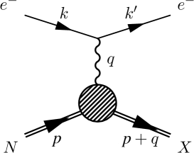
Figure 1: DIS, where $k$, $k^{\prime}$ represent the incoming, outgoing lepton momenta, $p$ is the momentum of the incoming nucleon of mass $M_{N}$, $q=k-k^{\prime}$ is the momentum transfer and $X$ represents the recoiling system.

The kinematics is such that $Q^{2}\equiv-q^{2}>0$; the invariant mass of $X$ is $M_{X}^{2}=(p+q)^{2}$ and the Bjorken variable, $x$, is defined by $x=Q^{2}/(2p\cdot q)$. Here we shall be mainly using the inverse Bjorken variable $\omega=1/x$. $x>0$ from kinematics and $M_{X}^{2}>M_{N}^{2}$ means that $x<1$ which translates to $1<\omega<\infty$ as the physical region. The square of the amplitude can be factorised into a calculable leptonic tensor together with an unknown hadronic tensor, $W_{\mu\nu}$, given by

$$W_{\mu\nu}\equiv{1\over 4\pi}\int d^{4}z\,e^{iq\cdot z}\rho_{ss^{\prime}}\,{}_{\rm rel}\langle p,s^{\prime}|[J_{\mu}^{\dagger}(z),J_{\nu}(0)]|p,s\rangle_{\rm rel}\,,$$ (1)

where $J_{\mu}$ is the electromagnetic current ($\gamma$) and for unpolarised nucleons we have $\rho_{ss^{\prime}}=\delta_{ss^{\prime}}/2$. The tensor has the Lorentz decomposition

$$W_{\mu\nu}=\left(-\eta_{\mu\nu}+{q_{\mu}q_{\nu}\over q^{2}}\right)F_{1}(x,Q^{2})+\left(p_{\mu}-{p\cdot q\over q^{2}}q_{\mu}\right)\left(p_{\nu}-{p\cdot q\over q^{2}}q_{\nu}\right){F_{2}(x,Q^{2})\over p\cdot q}\,,$$ (2)

with structure functions $F_{1}(x,Q^{2})$ and $F_{2}(x,Q^{2})$. It is useful to relate the $W_{\mu\nu}$ scattering amplitude to the forward Compton scattering amplitude, $T_{\mu\nu}$, depicted in the LH panel of Fig. 2, as this is a correlation function

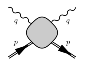
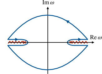
Figure 2: LH panel: The forward Compton Amplitude. RH panel: The analytic structure for ${\cal F}_{1}$ – branch cuts starting from $\omega=\pm 1$, together with the contour used for the dispersion relation.

and so more amenable to lattice QCD or other calculational methods. The definition parallels that of $W_{\mu\nu}$

$$T_{\mu\nu}(p,q)\equiv i\int d^{4}z\,e^{iq\cdot z}\rho_{ss^{\prime}}\,{}_{\rm rel}\langle p,s^{\prime}|T(J_{\mu}^{\dagger}(z)J_{\nu}(0))|p,s\rangle_{\rm rel}$$ (3)

$$= \left(-\eta_{\mu\nu}+{q_{\mu}q_{\nu}\over q^{2}}\right){\cal F}_{1}(\omega,Q^{2})+\left(p_{\mu}-{p\cdot q\over q^{2}}q_{\mu}\right)\left(p_{\nu}-{p\cdot q\over q^{2}}q_{\nu}\right){{\cal F}_{2}(\omega,Q^{2})\over p\cdot q}\,,$$

with corresponding structure functions ${\cal F}_{1}(\omega,Q^{2})$, ${\cal F}_{2}(\omega,Q^{2})$. Due to the time ordering in its definition it is a correlation function. These are related via the Optical theorem to the hadronic tensor structure functions by ${\rm Im}{\cal F}_{1}(\omega,Q^{2})=2\pi F_{1}(x,Q^{2})$ (and similarly for $F_{2}$, however in this talk we shall concentrate on $F_{1}$). Photon crossing symmetry $N\to\bar{N}$ means that ${\cal F}_{1}$ is symmetric under $\omega\to-\omega$ (while ${\cal F}_{2}$ is anti-symmetric). The analytic structure, e.g. [7], is thus given in the RH plot of Fig. 2. Analyticity properties (including using the Schwarz reflection principle across the branch cut) then give a once subtracted dispersion relation

$${\cal F}_{1}(\omega,Q^{2}) = {2\omega\over\pi}\int_{1}^{\infty}d\omega^{\prime}\left[{{\rm Im}{\cal F}_{1}(\omega^{\prime},Q^{2})\over\omega^{\prime}(\omega^{\prime}-\omega-i\epsilon)}-{{\rm Im}{\cal F}_{1}(\omega^{\prime},Q^{2})\over\omega^{\prime}(\omega^{\prime}+\omega-i\epsilon)}\right]+{\cal F}_{1}(0,Q^{2})$$ (4)

$$= \underbrace{4\omega^{2}\int_{0}^{1}dx^{\prime}{x^{\prime}F_{1}(x^{\prime},Q^{2})\over 1-x^{\prime\,2}\omega^{2}-i\epsilon}}_{\overline{\cal F}_{1}(\omega,Q^{2})}+\underbrace{{\cal F}_{1}(0,Q^{2})}_{\rm once\,\,subtracted}\,.$$

(Replacing $x^{\prime}F_{1}$ by $F_{2}$ with no subtraction gives the equivalent dispersion relation for $F_{2}$.) As long as we are in the unphysical region $|\omega|<1\Longleftrightarrow M_{X}^{2}<M_{N}^{2}$, i.e. below elastic threshold, there is no singularity in previous integral the time ordering is irrelevant, so the $i\epsilon$ in eq. (4) can be dropped. The Minkowski and Euclidean amplitudes are then identical which as we shall see in section (3) will eventually allow a direct lattice QCD computation. Physically $|\omega|<1$ means states propagating between currents cannot go on-shell. Taylor expanding the denominator in eq. (4) then gives

$${\overline{\cal F}}_{1}(\omega,Q^{2})=2\sum_{n=1}^{\infty}\omega^{2n}M^{(1)}_{2n}(Q^{2})\,,\quad\mbox{where}\quad M^{(1)}_{2n}(Q^{2})=2\int_{0}^{1}dx^{\prime}\,x^{\prime\,2n-1}F_{1}(x^{\prime},Q^{2})$$ (5)

are the Mellin moments of $F_{1}$. Furthermore for the numerical results considered later we set $\mu=\nu=z$, $p_{z}=q_{z}=0$ giving

$$T_{33}(p,q)={\overline{\cal F}}_{1}(\omega,Q^{2})=2\sum_{n=1}^{\infty}\omega^{2n}M^{(1)}_{2n}(Q^{2})\,.$$ (6)

So from Compton amplitude data we can directly extract the Mellin moments. The positivity of the cross section means that $F_{1}>0$ or $M^{(1)}_{2}\geq M^{(1)}_{4}\geq\ldots M^{(1)}_{2n}\geq\ldots>0$ so the expected shape of the Compton amplitude in the unphysical region for fixed $Q^{2}$ is simply an increasing polynomial function of $\omega^{2}$.

3 The Feynman–Hellmann approach

The task now is to compute the (Euclidean) Compton amplitude and in particular that given in eq. (6). A direct lattice QCD computation of the path integral for the necessary 4-point correlation function is complicated as there are many diagrams to compute. As an alternative we shall use the Feynman–Hellmann approach here.

We now sketch a derivation of the procedure. Consider the $2$-point nucleon correlation function

$$C_{fi\,\lambda}(t;\vec{p},\vec{q})={}_{\lambda}\langle 0|\underbrace{\hat{\tilde{B}}_{N_{f}}(0;\vec{p})}_{\rm Sink:\,momentum}\hat{S}(\vec{q})^{t}\underbrace{\hat{\bar{B}}_{N_{i}}(0,\vec{0})}_{\rm Source:\,spatial}|0\rangle_{\lambda}\,,$$ (7)

where $\hat{S}$ is the $\vec{q}$-dependent transfer matrix $\hat{S}(\vec{q})=\exp{(-\hat{H}(\vec{q}))}$ in the presence of a perturbed Hamiltonian

$$\hat{H}(\vec{q})=\hat{H}_{0}-\sum_{\alpha}\lambda_{\alpha}\hat{\tilde{{\cal O}}}_{\alpha}(\vec{q})\,,$$ (8)

where

$$\hat{\tilde{{\cal O}}}_{\alpha}(\vec{q})=\int_{\vec{x}}\left(\hat{O}_{\alpha}(\vec{x})e^{i\vec{q}\cdot\vec{x}}+\hat{O}_{\alpha}^{\dagger}(\vec{x})e^{-i\vec{q}\cdot\vec{x}}\right)$$ (9)

is a Hermitian operator. $\lambda$ can be taken as a real positive parameter. Using time dependent perturbation theory via the Dyson Series, namely the operator expansion, regarding $\hat{B}$ as ‘small’

$$e^{t(\hat{A}+\hat{B})}=e^{t\hat{A}}+\int_{0}^{t}dt^{\prime}\,e^{(t-t^{\prime})\hat{A}}\,\hat{B}\,e^{t^{\prime}\hat{A}}+\int_{0}^{t}dt^{\prime}\,\int_{0}^{t^{\prime}}dt^{\prime\prime}\,e^{(t-t^{\prime})\hat{A}}\,\hat{B}\,e^{(t^{\prime}-t^{\prime\prime})\hat{A}}\,\hat{B}e^{t^{\prime\prime}\hat{A}}+O(\hat{B}^{3})\,,$$ (10)

and inserting complete sets of unperturbed states

$$\sum_{\vec{p}}|N(\vec{p})\rangle\langle N(\vec{p})|+\sum_{E_{X}(\vec{p}_{X})>E_{N}(\vec{p})}|X(\vec{p}_{X}))\rangle\,\langle X(\vec{p}_{X})|=1\,,$$ (11)

appropriately gives after some algebra the factorised result

$$C_{fi\,\lambda}(t;\vec{p},\vec{q})={}_{\lambda}\langle 0|\hat{\tilde{B}}_{N_{f}}(\vec{p})|N(\vec{p})\rangle\times{}_{\lambda}\langle N(\vec{p})|\hat{\bar{B}}_{N_{i}}(\vec{0})|0\rangle_{\lambda}\times e^{-E_{N\,\lambda}(\vec{p},\vec{q})t}+\ldots\,,$$ (12)

where as this equation suggests we have taken the lowest state $|N(\vec{p})\rangle$ to be well separated from other states. Furthermore we have defined ${}_{\lambda}\langle N(\vec{p})|$ as

$${}_{\lambda}\langle N(\vec{p})|=\langle N(\vec{p})|+\lambda_{\alpha}\,\sum_{E_{Y}(\vec{p}_{Y})>E_{N}(\vec{p})}{\langle N(\vec{p})|\hat{\tilde{{\cal O}}}_{\alpha}(\vec{q})|Y(\vec{p}_{Y})\rangle\over E_{Y}(\vec{p}_{Y})-E_{N}(\vec{p})}\,\langle Y(\vec{p}_{Y})|+O(\lambda^{2})\,.$$ (13)

(We do not give the $O(\lambda^{2})$ term here.) While the final nucleon operator, $\hat{\tilde{B}}_{N_{f}}(\vec{p})$, has a definite momentum and so just picks out one state, the initial nucleon operator, $\hat{B}_{N_{i}}(\vec{0})$, being at position $\vec{x}=\vec{0}$ contains all momenta and states (indicated here by the sum over $|X(\vec{p}_{X})\rangle$). For the matrix elements that appear in the modified energy in eq. (12), rather than writing them in terms of the operator $\hat{\tilde{{\cal O}}}_{\alpha}$ we first use $\hat{O}(\vec{x})=e^{-i\hat{\vec{p}}\cdot\vec{x}}\,\hat{O}(\vec{0})\,e^{i\hat{\vec{p}}\cdot\vec{x}}$ on the relevant term to give

$$\langle X(\vec{p}_{X})|\hat{\tilde{{\cal O}}}_{\alpha}(\vec{q})|N(\vec{p})\rangle=\langle X(\vec{p}_{X})|\hat{O}_{\alpha}(\vec{0})|N(\vec{p})\rangle\,\delta_{\vec{p}_{X},\vec{p}+\vec{q}}+\langle X(\vec{p}_{X})|\hat{O}_{\alpha}^{\dagger}(\vec{0})|N(\vec{p})\rangle\,\delta_{\vec{p}_{X},\vec{p}-\vec{q}}\,,$$ (14)

so matrix elements step up or down in $\vec{q}$. As this is also valid for $X=N$ then the $O(\lambda)$ term vanishes ($\vec{q}\not=\vec{0}$). Generalising each $\lambda$ inserts another $\hat{\tilde{{\cal O}}}$ into the matrix element, so we need an even number of $\lambda$s, i.e. odd powers of $\lambda$ vanish. This gives finally

$$E_{N\,\lambda}(\vec{p},\vec{q}) = E_{N}(\vec{p})-\sum_{E_{X}(\vec{p}\pm\vec{q})>E_{N}(\vec{p})}\left[{|\langle X(\vec{p}+\vec{q})|\lambda_{\alpha}\hat{O}_{\alpha}(\vec{0})|N(\vec{p})\rangle|^{2}\over E_{X}(\vec{p}+\vec{q})-E_{N}(\vec{p})}\right.$$

$$\left.\hskip 108.405pt+{|\langle X(\vec{p}-\vec{q})|(\lambda_{\alpha}\hat{O}_{\alpha}(\vec{0}))^{\dagger}|N(\vec{p})\rangle|^{2}\over E_{X}(\vec{p}-\vec{q})-E_{N}(\vec{p})}\right]+O(\lambda^{3})\,.$$

We need $E_{N}(\vec{p}\pm\vec{q})>E_{N}(\vec{p})$ ($X=N$ is the worst case) giving $-1<\omega<1$ with $\omega=2\vec{p}\cdot\vec{q}/\vec{q}^{2}$. This is the usual definition of $\omega$ (with $q_{0}=0$), which is in the safe unphysical region.

What has all this to do with the Compton Amplitude? We now interpret this result and relate it to the Compton Amplitude. Considering its Minkowski (${\cal M}$) definition again, eq. (3), and again inserting a complete set of states for $t>0$ and $t<0$ with the appropriate $i\epsilon$ prescription

$$T^{\rm\scriptscriptstyle({\cal M})}_{\mu\nu}(p,q) = \sum_{X}\left[{\langle X(\vec{p}+\vec{q})|\hat{O}_{\mu}(\vec{0})|N(\vec{p})\rangle^{*}\,\langle X(\vec{p}+\vec{q})|\hat{O}_{\nu}(\vec{0})|N(\vec{p})\rangle\over E_{X}(\vec{p}+\vec{q})-E_{N}(\vec{p})-q^{0}-i\epsilon}\right.$$ (16)

$$\left.\hskip 25.29494pt+{\langle X(\vec{p}-\vec{q})|\hat{O}^{\dagger}_{\nu}(\vec{0})|N(\vec{p})\rangle^{*}\langle X(\vec{p}-\vec{q})|\hat{O}^{\dagger}_{\mu}(\vec{0})|N(\vec{p})\rangle\over E_{X}(\vec{p}-\vec{q})-E_{N}(\vec{p})+q^{0}-i\epsilon}\right]\,.$$

Comparing with the previous result of eq. (3) if we set $q^{0}=0$ and choose the $\vec{p},\vec{q}$ geometry so that $E_{X}(\vec{p}\pm\vec{q})>E_{N}(\vec{p})$, i.e. $-1<\omega<1$ then we can also drop the $i\epsilon$ which gives

$$E_{N\,\lambda}(\vec{p},\vec{q})=E_{N}(\vec{p})-{\lambda_{\alpha}^{*}\lambda_{\beta}\over{}_{\rm rel}\langle N(\vec{p})|N(\vec{p}\rangle_{\rm rel}}T^{\rm\scriptscriptstyle({\cal M})}_{\alpha\beta}((E_{N}(\vec{p}),\vec{p}),(0,\vec{q}))+O(\lambda^{4})\,.$$ (17)

As $T^{\rm\scriptscriptstyle({\cal M})}_{\alpha\beta}(p,q)^{*}=T^{\rm\scriptscriptstyle({\cal M})}_{\beta\alpha}(p,q)$ then the real part of Compton amplitude is symmetric (unpolarised case with $\lambda$ real) while the imaginary part is anti-symmetric (polarised with $\lambda$ complex).

For the DIS case considered here in eq. (6) where $\mu=\nu=z$; $p_{z}=q_{z}=0$, giving $T_{33}(p,q)={\cal F}_{1}(\omega,Q^{2})$. So with $O_{\alpha}\to J_{z}$ we have finally

$$\Delta E_{N\,\lambda}(\vec{p},\vec{q})\equiv E_{N\,\lambda}(\vec{p},\vec{q})-E_{N}(\vec{p})=-{\lambda_{z}^{2}\over 2E_{N}(\vec{p})}{\cal F}_{1}(\omega,Q^{2})+O(\lambda^{4})\,,$$ (18)

writing the relativistic normalisation explicitly.

4 The Lattice

We now briefly describe some lattice details. In the Lagrangian in the path integral we add the equivalent perturbation

$${\cal L}(x)={\cal L}_{0}(x)+2\lambda_{z}\cos(\vec{q}\cdot\vec{x})J_{z}(x)\,,$$ (19)

where rather than considering the complete electromagnetic current we take the vector current $J^{(q)}_{\mu}$ to be either $Z_{V}\bar{u}\gamma_{\mu}u$ (where $q\to u$) or $Z_{V}\bar{d}\gamma_{\mu}d$ ($q\to d$). $Z_{V}$ has been previously determined. We only modify the propagators for the valence $u/d$ quarks in $\lambda$. So there are no quark-line disconnected terms considered here. To include this would require at least very expensive dedicated configuration generation.

More specifically we consider $2+1$ quark mass degenerate flavours on a $N_{S}^{3}\times N_{T}=32^{3}\times 64$ lattice with a spacing $a\sim 0.074\,\mbox{fm}$. (Technically $\beta=5.50$, $\kappa_{l}=0.120900$, $l=u$, $d$ or $s$ giving $m_{\pi}\sim 470\,\mbox{MeV}$ and $m_{\pi}L\sim 5.4$ where $L=aN_{S}$.) For more details of the action and configuration generation see [9]. Apart from $\lambda_{z}=0$, we use $4$ values of $\lambda_{z}$, namely $\pm 0.0125$, $\pm 0.025$. $Q^{2}$ has $5$ values in the range between $3$ and $7\,\mbox{GeV}^{2}$ and we make $\sim O(10^{4})$ measurements for each $\lambda_{z}$, $Q^{2}$ pair (varying $\vec{p}$ is numerically cheap as it is not part of the source, and hence not connected with the numerically expensive fermion matrix inversion).

4.1 Kinematic coverage

We now briefly discuss the possible kinematic coverage, which is sketched in the LH panel of Fig 3.

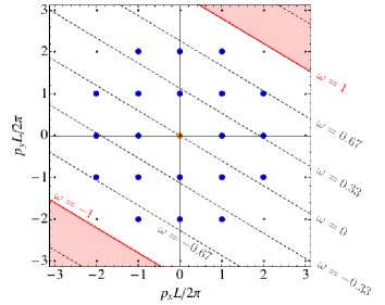
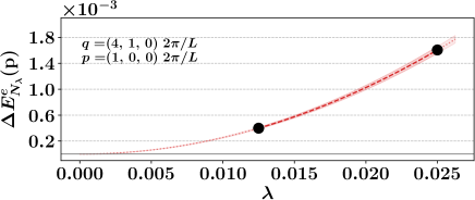
Figure 3: LH panel: The allowed kinematic possibilities for $\vec{p}$ given $\vec{q}=2\pi/L(3,5,0)$, where $L=32a$. Lines of constant $\omega=(2/34)(3n_{x}+5n_{y})$ are shown dashed. The blue dots give the allowed momenta. RH panel: A plot of $\Delta E_{N\,\lambda}$ against $\lambda_{z}$ for $\vec{q}=2\pi/L(4,1,0)$ and $\vec{p}=2\pi/L(1,0,0)$.

As an example consider fixed $\vec{q}=(2\pi/L)\,(3,5,0)$. We can access different $\omega$ by varying the nucleon momenta $\vec{p}=(2\pi/L)\vec{n}$ as $\omega=2\vec{p}\cdot\vec{q}/\vec{q}^{2}=(2/34)(3n_{x}+5n_{y})$. Thus for a given constant $\omega$ we have a linear relationship between $n_{y}$ and $n_{x}$ as shown by the lines in the LH panel of Fig. 3. The blue dots give allowed values of $\vec{p}$.

To extract energy shifts, $\Delta E_{N\,\lambda}$, for each $\lambda_{z}$ we form ratios, $R_{\lambda}$ which isolate the $O(\lambda_{z}^{2})$ term

$$R_{\lambda}={C_{NN\,+\lambda_{z}}(t)\,C_{NN\,-\lambda_{z}}(t)\over C_{NN\,0}(t)^{2}}=A_{\lambda}(\vec{p},\vec{q})\,e^{-2\Delta E_{N\,\lambda}(\vec{p},\vec{q})}+\ldots\,.$$ (20)

After extracting $\Delta E_{N\,\lambda}$, this is plotted against $\lambda_{z}$. An example is shown in the RH panel of Fig. 3 for $\vec{q}=2\pi/L(4,1,0)$, $\vec{p}=2\pi/L(1,0,0)$ (giving $Q^{2}=4.7\,\mbox{GeV}^{2}$). A quadratic fit gives from eq. (18) the structure function, ${\cal F}_{1}(\omega,Q^{2})$, at one value of $\omega$. Repeating this for various values of $\vec{p}$ and $\vec{q}$ gives the complete structure function of $\omega$ and $Q^{2}$.

4.2 Results

In Fig. 4 we show ${\cal F}_{1}(\omega,Q^{2})$ as a

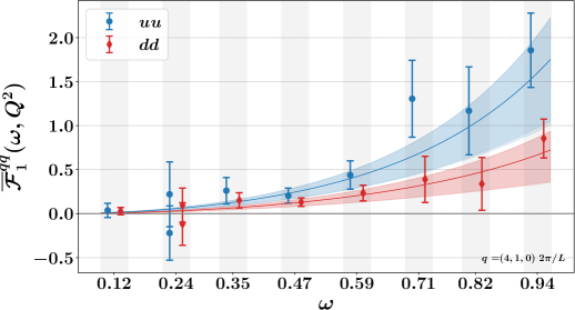
Figure 4: $\omega$ dependence of ${\cal F}_{1}(\omega,Q^{2})$ for $Q^{2}=4.7\,\mbox{GeV}^{2}$. The blue circles are for $J_{z}^{(u)}$, the red diamonds for $J_{z}^{(d)}$. The fits, blue and red lines with errors given by shaded region are described in the text. The points are slightly shifted for clarity.

function of $\omega$ for $Q^{2}=4.7\,\mbox{GeV}^{2}$ for $J^{(u)}_{z}$ and $J^{(d)}_{z}$ separately. This figure is our main result. We now mention some further consequences from this result. From eq. (5) we can make a fit to ${\cal F}_{1}(\omega,Q^{2})$ to determine the (low) Mellin moments. We have the constraints $M^{(1)}_{2}\geq M^{(1)}_{4}\geq\ldots\geq M^{(1)}_{2n}\geq\ldots>0$ for $u$, $d$ separately and so we have implemented a Bayesian procedure (likelihood with priors as constraints). These are also shown in the LH panel of Fig. 5 for $n=6$.

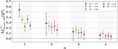
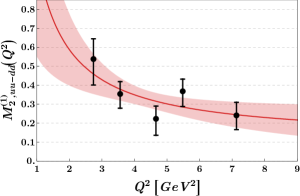
Figure 5: LH panel: The first $5$ isovector moments $M^{(1)}_{2n;u-d}(Q^{2})$ (using $J^{(u)}_{z}-J^{(d)}_{z}$ for various $Q^{2}$ values). RH panel: The corresponding valence PDF for $M^{(1)}_{2;u-d}(Q^{2})$ $Q^{2}=2.7\,\mbox{GeV}^{2}$, together with the fit from eq. (21).

We note that the fall-off of the moments is as expected, however the second moment does not decrease as rapidly as expected from DIS.

Alternatively we can investigate the $Q^{2}$ dependence of a particular moment and investigate scaling and the existence of power corrections not restricted to the OPE and large $Q^{2}$ as shown in the RH panel of Fig. 5. We also made the naive fit

$$M^{(1)}_{2;u-d}(Q^{2})=M^{(1)}_{2;u-d}+{C_{2}^{(u-d)}\over Q^{2}}\,.$$ (21)

We concluded, [5, 11, 10], that we need $Q^{2}\mathrel{\hbox to0.0pt{\lower 4.0pt\hbox{\hskip 1.0pt$\sim$}\hss}\raise 1.0pt\hbox{$>$}}16\,\mbox{GeV}^{2}$ to reliably extract moments at a scale of $\mu=2\,\mbox{GeV}$.

Is it possible to reconstruct the Form Factor, $F_{1}$ or indeed the PDF? This, of course, would be the ultimate goal. From eq. (4) we have

$$T_{33}(\omega,Q^{2})=\omega\int_{0}^{1}dx\,K(x\omega)\,F_{1}(x,Q^{2})\,,\quad\mbox{where}\quad K(\xi)=4\,{\xi\over 1-\xi^{2}}\,.$$ (22)

This is a Fredholm integral equation and so an inverse problem, which is ill defined. Presently with this data, we have first made the ansatz

$$F_{1}(x,Q^{2})\equiv ap_{\rm val}(x;b,c)=a\,{\Gamma(b+c+3)\over\Gamma(b+2)\Gamma(c+1)}\,x^{b}(1-x)^{c}\,,$$ (23)

(normalised to $\int_{0}^{1}dx\,xp_{\rm val}=1$). Again with a Bayesian implementation, we find typical results as in Fig. 6

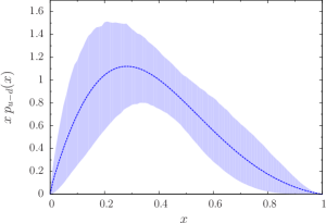
Figure 6: The valence PDF, $p_{\rm val}^{(u-d)}$ for $Q^{2}=2.7\,\mbox{GeV}^{2}$.

here for $Q^{2}=2.7\,\mbox{GeV}^{2}$. The general shape is okay (the parton model would give a $\delta$-function at $x=1/3$, which is smeared out by QCD corrections).

5 Further applications

Finally we briefly mention some more applications of this method.

5.1 The $O(\lambda)$ term

We previously showed that the $O(\lambda)$ terms vanish if $\vec{q}\not=\vec{0}$. However for $\vec{q}=\vec{0}$ then it is possible to determine the baryon charges. For example in [12] the tensor charge of octet baryons was determined.

However we can escape this constraint if there is an degeneracy when two (or more) states have the same energy. Then we now have a matrix of states $M_{rs}=\langle N(\vec{p}_{r})|\hat{\tilde{O}}(\vec{q})|N(\vec{p}_{s})\rangle$ (where $r,s=1\,,\ldots\,,d_{S}$, where $d_{S}$ is the number of degenerate states). As before the diagonal elements vanish, but the off-diagonal do not. This can be diagonalised to give $\Delta E_{N\,\lambda}$. In [13] this was investigated (for $d_{S}=2$ in the Breit frame) and applied to form factors and scattering over a large range of $Q^{2}$.

5.2 The $O(\lambda^{2})$ term

While most of our present effort has been directed at the forward Compton amplitude, we have also started to investigate Off-forward Compton Amplitude (OFCA) and GPDs in [14] where we described the fomalism and determined the two lowest moments.

5.3 Possible future perspectives

Possible future perspectives include Spin dependent Structure functions and Form factors as indicated in eq. (17), electromagnetic corrections to the proton – neutron mass splitting $M_{p}-M_{n}=\delta M^{\gamma}+\delta M^{m_{d}-m_{u}}$ via the Cottingham formula

$$\delta M^{\gamma}={i\over 2M}{\alpha_{em}\over(2\pi)^{2}}\int{\eta^{\mu\nu}\over q^{2}+i\epsilon}T_{\mu\nu}(p,q)\,,$$ (24)

and mixed currents, for example neutrino-nucleon charged weak current $\nu N\to eX$ or $eN\to\nu X$

$$W^{\mu\nu} \equiv {1\over 4\pi}\int d^{4}z\,e^{iq\cdot z}\rho_{ss^{\prime}}\,{}_{\rm rel}\langle p,s^{\prime}|[J^{\mu}_{\rm em}(z),J^{\nu}_{W,A}(0)]|p,s\rangle_{\rm rel}$$ (25)

$$= -i\epsilon^{\mu\nu\alpha\beta}\,{q_{\alpha}p_{\beta}\over{2p\cdot q}}F_{3}(x,Q^{2})\,,$$

where $J^{\nu}_{W,A}=\bar{u}\gamma_{\nu}\gamma_{5}d$ the axial part of the weak charged current.

A potential problem is including quark-line-disconnected matrix elements. This needs purpose generated configurations with the fermion determinant also containing the $\lambda$ term. For (H)MC for the probability definition of the action also need a real determinant so fermion matrix must be $\gamma_{5}$-Hermitian which means that $\lambda^{V}$ and $\lambda^{A}$ have to be imaginary (while $\lambda^{S}$, $\lambda^{P}$ and $\lambda^{T}$ are all real). In this case $\Delta E_{\lambda}$ develops an imaginary part. (This is not a problem for the valence sector, as this is just an inversion of a matrix.) Simulations are however possible and this was investigated in [15] (at $O(\lambda)$) for the disconnected contributions to the spin of the nucleon.

6 Conclusions

We have described here a new versatile approach for the computation of matrix elements only involving computation of $2$-point correlation functions rather than $3$-pt or $4$-pt which is able to compute Compton amplitudes and structure function moments. Advantages include longer source-sink separations – so less excited states contamination and overcoming fierce operator mixing / renormalisation issues.

References

- [1] M. Diehl, Introduction to GPDs and TMDs, Eur. Phys. J. A 52 (2016) 149, [arXiv:1512.01328].
- [2] M. Göckeler et al., A Lattice determination of moments of unpolarised nucleon structure functions using improved Wilson fermions Phys. Rev. D 71 (2005) 114511, [arXiv:hep-ph/0410187].
- [3] K. Cichy and M. Constantinou, A guide to light-cone PDFs from Lattice QCD: an overview of approaches, techniques and results, Adv. High Energy Phys. 2019 (2019) 3036904, [arXiv:1811.07248].
- [4] A. J. Chambers et al., Nucleon Structure Functions from Operator Product Expansion on the Lattice, Phys. Rev. Lett. 118 (2017) 242001, [arXiv:1703.01153].
- [5] K. U. Can et al., Lattice QCD evaluation of the Compton amplitude employing the Feynman-Hellmann theorem, Phys. Rev. D 102 (2020) 114505, [arXiv:2007.01523].
- [6] K. U. Can et al., Investigating the low moments of the nucleon structure functions in lattice QCD, PoS LATTICE2021 (2021) 324, arXiv:2110.01310.
- [7] S. Gasiorowicz, Elementary Particle Physics, Wiley 1966.
- [8] F. Hagelstein and V. Pascalutsa, The subtraction contribution to the muonic-hydrogen Lamb shift: A point for lattice QCD calculations of the polarizability effect, Nucl. Phys. A 1016 (2021) 122323, [arXiv:2010.11898].
- [9] W. Bietenholz et al., Flavour blindness and patterns of flavour symmetry breaking in lattice simulations of up, down and strange quarks, Phys. Rev. D 84 (2011) 054509, [arXiv:1102.5300].
- [10] R. Horsley et al., Structure functions from the Compton amplitude, PoS LATTICE2019 (2020) 137, [arXiv:2001.05366].
- [11] A. Hannaford-Gunn et al., Scaling and higher twist in the nucleon Compton amplitude, PoS LATTICE2019 (2019) 278, [arXiv:2001.05090].
- [12] R. E. Smail et al., Tensor Charges and their Impact on Physics Beyond the Standard Model, PoS LATTICE2021 (2021) 494, arXiv:2112.05330.
- [13] A. J. Chambers et al., Electromagnetic form factors at large momenta from lattice QCD, Phys. Rev. D 96 (2017) 114509, [arXiv:1702.01513].
- [14] A. Hannaford-Gunn et al., Generalised parton distributions from the off-forward Compton amplitude in lattice QCD, Phys. Rev. D 105 (2022) 014502, [arXiv:2110.11532].
- [15] A. J. Chambers et al., Disconnected contributions to the spin of the nucleon, Phys. Rev. D 92 (2015) 114517, [arXiv:1508.06856].
- [16] T. R. Haar, Y. Nakamura and H. Stüben, An update on the BQCD Hybrid Monte Carlo program, EPJ Web Conf. 175 (2018) 14011, [arXiv:1711.03836].
- [17] R. G. Edwards and B. Joó, The Chroma software system for lattice QCD, Nucl. Phys. B Proc. Suppl. 140 (2005) 832, [arXiv:hep-lat/0409003].