Photochemical Runaway in Exoplanet Atmospheres: Implications for Biosignatures
Abstract
About 2.5 billion years ago, microbes learned to harness plentiful solar energy to reduce CO2 with H2O, extracting energy and producing O2 as waste. O2 production from this metabolic process was so vigorous that it saturated its photochemical sinks, permitting it to reach “runaway” conditions and rapidly accumulate in the atmosphere despite its reactivity. Here we argue that O2 may not be unique: diverse gases produced by life may experience a “runaway” effect similar to O2. This runaway occurs because the ability of an atmosphere to photochemically cleanse itself of trace gases is generally finite. If produced at rates exceeding this finite limit, even reactive gases can rapidly accumulate to high concentrations and become potentially detectable. Planets orbiting smaller, cooler stars, such as the M dwarfs that are the prime targets for the James Webb Space Telescope (JWST), are especially favorable for runaway due to their lower UV emission compared to higher-mass stars. As an illustrative case study, we show that on a habitable exoplanet with an H2-N2 atmosphere and net surface production of NH3 orbiting an M dwarf (the “Cold Haber World” scenario), the reactive biogenic gas NH3 can enter runaway, whereupon an increase in the surface production flux of one order of magnitude can increase NH3 concentrations by three orders of magnitude and render it detectable by JWST in just two transits. Our work on this and other gases suggests that diverse signs of life on exoplanets may be readily detectable at biochemically plausible production rates.
1 Introduction
The detection of biologically produced gases indicative of life (”biosignature gases”) in rocky exoplanet atmospheres is a key goal of exoplanet science. Yet simulations predict that observations of even the main atmospheric gases will be challenging, mainly due to the small sizes of rocky planets and their atmospheres. Observations of trace biosignature gases will be even more challenging (Morley et al., 2017; Batalha et al., 2018; Lustig-Yaeger et al., 2019). On modern Earth, most products of biology do not accumulate to atmospheric concentrations that can be remotely detected over interstellar distances, because either their production rates are low, or they are too photochemically reactive, or both (Kasting et al., 2014; Rugheimer & Kaltenegger, 2018; Kaltenegger, 2017). Photochemical reactivity is also predicted to restrict diverse biosignature gases to undetectably low concentrations for exoplanets dissimilar to modern Earth as well, including gases for which efficient abiotic ”false positive” production mechanisms have not yet been identified (e.g., Domagal-Goldman et al. 2011; Sousa-Silva et al. 2020; Zhan et al. 2021).
A notable exception to the pessimism regarding biosignature gases is oxygen (O2). On modern Earth, O2 constitutes 21% of modern Earth’s atmosphere by volume. Thanks to its high abundance, O2 and its photochemical by-product O3 are accessible to detection by next-generation telescopes for Earth-twin exoplanets orbiting small, nearby stars, though even these observations will be challenging (Rodler & López-Morales, 2014; Reinhard et al., 2017; Kawashima & Rugheimer, 2019; Fauchez et al., 2020). While not unambiguous as a biosignature, the detectability of O2 and its by-product O3 make oxygen a prime target for biosignature searches (Meadows et al., 2018). However, the oxygenation of Earth’s atmosphere was not straightforward. Earth’s atmosphere was anoxic for approximately the first half of its history, and up to hundreds of millions of years may have elapsed between the emergence of biological O2 production and its accumulation in the atmosphere to ppmv levels. O2’s accumulation to a dominant atmospheric gas ( by volume) is even more recent, within the last billion years (Lyons et al., 2014). This is because O2 is very reactive, and readily reacted with reductants in the atmosphere of early Earth. At low surface production fluxes, such reactions photochemically confine the atmospheric concentration of O2 to undetectably low levels. However, when the net production flux of O2 exceeded the supply of reductants to the atmosphere on a sustained basis, O2 atmospheric concentrations rose dramatically, until ultimately limited by surface processes (Goldblatt et al., 2006; Zahnle et al., 2006; Daines et al., 2017).
O2 may not be unique. At high enough production rates, diverse gases may come to saturate their photochemical sinks and increase rapidly in concentration as a function of surface flux. We term this general process ”photochemical runaway,” after the prototypical ”CO runaway” (Zahnle, 1986; Kasting, 2014). The term “runaway” is often used to describe a time-dependent phenomenon, but despite its etymology, photochemical runaway refers to an essentially stationary effect111While primarily a steady-state, stationary effect, we note in passing there is an element of time dependence in runaway, because it may take time to saturate the surface, as occurred with O2.. The photochemical runaway of CO has been the most studied in the literature, but photochemical runaways of other gases (e.g., CH4, PH3, and isoprene) have also been briefly reported (Kasting, 1990; Pavlov et al., 2003; Kharecha et al., 2005; Segura et al., 2005; Schwieterman et al., 2019; Sousa-Silva et al., 2020; Zhan et al., 2021).
The physical mechanism underlying photochemical runaway is that the photochemical sinks limiting trace gas accumulation in the atmosphere are finite, and can be overwhelmed with high gas production. More fully, photochemistry generally controls the removal of biogenic gases from habitable planet atmospheres, because thermochemistry is generally slow at habitable temperatures. Photochemical removal of atmospheric gases is mediated by UV photons, either directly, via photolysis, or indirectly, via reactions with radicals produced by photolysis (Catling & Kasting, 2017; Grenfell et al., 2018). As the supply of UV photons and the supply of photolyzable substrates are both finite, the ability of the atmosphere to photochemically cleanse itself is also finite. If emitted at fluxes exceeding this finite threshold, gases can overwhelm the photochemical controls on their accumulation and rapidly increase in concentration, until they are ultimately limited by other processes, e.g. surface uptake by biogeochemical sinks.
Photochemical runaway is important because it suggests that even reactive biosignature gases can accumulate to high, detectable concentrations at biochemically plausible fluxes, particularly for planets orbiting smaller, cooler stars with lower UV emission compared to higher-mass stars. Photochemical runaways are nonlinear: past the runaway threshold, a small increase in surface emission flux may result in dramatic increases in atmospheric concentration and hence detectability. The precise threshold for runaway varies by gas and planet scenario, but is often, though not always, set by the UV output of the host star. This is because it is UV photons that ultimately mediate the photochemical removal of atmospheric gases (Segura et al., 2005; Zahnle et al., 2006). Fortuitously for observations, this suggests that planets orbiting M-dwarf stars are more prone to runaways compared to planets orbiting Sun-like stars, because of their lower emission of photolytic near-UV (NUV) radiation (Segura et al., 2005; Rugheimer et al., 2015). Older, cooler white dwarf stars should be similarly favorable for runaway due to their lower UV output (Kozakis et al. 2020; Lin et al. 2022). Due to the observational advantages derived from their small host stars, planets orbiting cool stars like M dwarfs and white dwarfs are the only plausible rocky planet targets for near-term atmospheric characterization via transmission spectroscopy. Thus, the planets most amenable to atmospheric characterization are also the most generally prone to runaways.
Photochemical runaway has been studied for individual gases as a photochemical phenomenon, but its observational implications, particularly for reactive biosignature gases, have not been made clear. Here, we study photochemical runaway as a general phenomenon, with emphasis on its observational implications. We illustrate the effect of photochemical runaway and its implications for trace gas detectability in exoplanet atmospheres by exploring the case study of NH3 runaway in an H2-N2 exoplanet atmosphere. We discuss the generality of photochemical runaway, showing that with the same photochemical model and reaction network, a broad range of gases in diverse planet scenarios, including non-H2 dominated atmospheres, can undergo runaway. We address literature concerns regarding the physicality of runaway, demonstrating that the previous blanket dismissal of runaway on thermodynamic grounds is not justified and interpreting the rise of O2 on Earth as an actualized example of photochemical runaway, giving empirical grounding to the theory. We close with a discussion of the observational implications and uncertainties of runaway.
2 Methods
We studied NH3 as a case study for photochemical runaway and its implications for the detectability of trace biosignature gases. To simulate NH3 runaway, we choose an H2-N2-dominated atmospheric scenario, corresponding to the Cold Haber World scenario (Seager et al., 2013a, b; Phillips et al., 2021) in which life would have a metabolic incentive for the high production of NH3. We model the photochemical runaway of NH3 in this planetary scenario (Section 2.1), the implications of runaway for the detectability of NH3 (Section 2.2), and its climate feedback (Section 2.3).
2.1 Photochemical Modeling
To calculate the concentration of NH3 as a function of surface emission flux, we employed the 1D photochemical model of Hu et al. (2012). The model is designed for the flexible exploration of atmospheres of varying redox state, and is fully detailed in Hu et al. (2012, 2013). In brief, the model calculates the composition of a rocky planet atmosphere in kinetic steady-state by solving the 1D continuity-transport equation. It encodes 111 CHNOS-bearing species linked by 900 chemical reactions, of which subsets can be flexibly specified to explore diverse atmospheric scenarios. The processes encoded by the model include surface emission, wet and dry deposition, eddy diffusion, molecular diffusion and diffusion-limited escape of H and H2, formation and deposition of S8 and H2SO4 aerosols, and photolysis; radiative transfer is computed via the delta two-stream approximation, including molecular absorption, Rayleigh scattering, and aerosol scattering and absorption. The model reproduces the trace gas compositions of the atmospheres of modern Earth and Mars, and has recently been intercompared with other models for the case of prebiotic Earth-analog exoplanets orbiting Sunlike stars(Ranjan et al., 2020). Relative to the original model, we have corrected the nm CO2 cross-sections, corrected the temperature dependence of the Henry’s Law constants used in the wet deposition calculation, and updated the H2O cross-sections to utilize the new measurements from Ranjan et al. (2020) (their ”extrapolation” prescription). Prior to utilizing the updated model, we confirmed that the model reproduces the atmospheric composition of Earth and Mars, as defined in Hu et al. (2012).
2.1.1 Photochemical Network
We build on the chemical network of the Hu et al. (2012) atmospheric benchmark scenarios. We expand our reaction network relative to the Hu et al. (2012) benchmark scenarios by including nitrogenous chemistry. While the chemistry of nitrogen-bearing molecules was encoded into the Hu model, these reactions were not included in the reaction network used to study the Hu et al. (2012) abiotic exoplanet benchmark scenarios, because nitrogenous chemistry was not their focus. As our focus is nitrogenous NH3, we instead include all nitrogenous chemistry encoded in the Hu model in our reaction network. We exclude reactions T45 and R92 of Hu et al. (2012) from our network, because they correspond to isomers of species in our model, and were originally included in error. Specifically, T45 refers to the thermal decay of HSOO and R92 refers to a reaction of CH2=C (Goumri et al., 1999; Laufer & Fahr, 2004); neither species is included in our model. We update the rate law for reaction R317 of Hu et al. (2012) (NH2 + CH4 NH3 + CH3), from cm3 s-1 (Möller & Wagner, 1984) to cm3 s-1 (Siddique et al., 2017). Finally, we correct the rate law for reaction R40 of Hu et al. (2012) (NH + OH NH2 + O) from cm3 s-1 to cm3 s-1 (Cohen & Westberg, 1991).
We follow Hu et al. (2012) in excluding reactions involving molecules containing carbons. We exclude the chemistry because the photochemistry of the higher hydrocarbons and their accompanying haze is poorly understood; we account for it in an ad hoc fashion as in Hu et al. (2012), i.e. by assigning a high deposition velocity of cm s-1 to C2H6. This means that our model is invalid in hazy atmospheric regimes, e.g. when the CH4/CO2 ratio exceeds in an N2-dominated atmosphere; we do not deploy our model in this regime. In total, our network encompasses 736 reactions linking 86 chemical species.
2.1.2 Stellar Irradiation
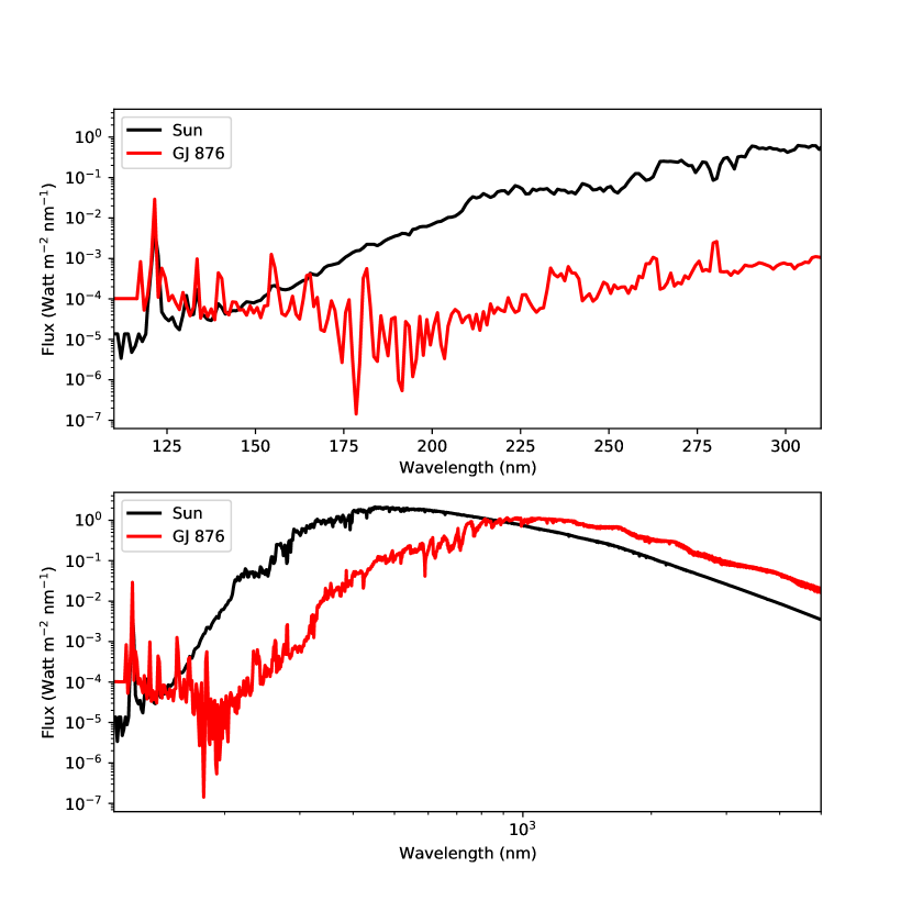
We consider irradiation from Sun-like stars and M dwarfs. We draw our irradiation spectrum for Sun-like stars from Hu et al. (2012), who in turn synthesized it from the Air Mass Zero reference spectrum produced by the American Society For Testing and Materials222https://www.nrel.gov/grid/solar-resource/spectra.html ( nm) and from the average quiet Sun emission spectrum of Curdt et al. (2004) ( nm). We represent M dwarf absorption spectra by that of GJ 876, and draw its spectrum from that synthesized by the MUSCLES333https://archive.stsci.edu/prepds/muscles/ collaboration based on telescopic measurements (v. 2.2; France et al. 2016; Youngblood et al. 2016; Loyd et al. 2016). We chose GJ 876 for its relatively well-characterized spectrum and for its low UV output relative to other M dwarfs with well-characterized spectra, which maximized the contrast with Sunlike stars to illustrate the impact of different UV irradiation fields. This low UV output means that calculations of biosignature gas buildup utilizing GJ 876 represent a favorable endmember scenario; this bias is counterbalanced by our expectation that the sample of M dwarfs with well-characterized UV radiation fields should be biased to stars with higher UV output, because these brighter stars are more amenable to observation. We follow Hu et al. (2012) in adopting a semimajor axis for the H2-dominated atmosphere of 1.6 AU for the solar instellation case (based on crude climate calculations), and we scale our GJ 876 spectra to the same total instellation.
2.1.3 Convergence Criteria
We require that the chemical variation timescale (Hu et al., 2012) of each species at each altitude with abundance exceeding 1 cm-3 be s. We adopt this unphysically stringent criteria, which corresponds to timescales far greater than the age of the universe, because we found that adopting less stringent criteria could sometimes lead to ”false minima” that did not correspond to the true steady-state solution. For example, the O2 instability as a function of boundary condition discussed in Section 2.1.4 would not have been detected for a less stringent timescale requirement, e.g. one corresponding to the age of the solar system. For each simulation, we verify stable convergence by rerunning the converged solutions.
We comment that it is particularly difficult to converge solutions according to these criteria when a gas enters runaway, particularly a photochemically reactive gas like NH3. We attribute this to the observation that when a gas enters runaway, it begins to photochemically reengineer the atmosphere, e.g. CO suppressing OH; O2 converting the atmosphere from near-neutral to strongly oxidizing (Appendix C). This makes the ”runaway regime” photochemically unstable, as the bulk atmospheric forcing is changing. After runaway is complete and the atmosphere has been reengineered, convergence becomes easier. We therefore consider our calculations most precise for surface fluxes much above or below the runaway threshold, while solutions in close vicinity to the runaway threshold are more likely sensitive to physical and numerical uncertainties (e.g., uncertainties in the photochemical network, Ranjan et al. 2020). In other words, we consider the high gas concentrations at production fluxes significantly exceeding the runaway threshold and the low gas concentrations at production fluxes significantly below the runaway threshold to be robust, but do not place much confidence in the precise mapping between surface fluxes and atmospheric concentrations right at the runaway threshold.
2.1.4 Planet Scenario
We construct our planet scenario by modifying the H2-dominated atmospheric benchmark scenario of Hu et al. (2012). This scenario corresponds to an atmosphere with bulk composition of 0.9 bar H2 and 0.1 bar N2, overlying an abiotic but habitable planet, with a surface temperature of 288 K, an ocean, and Earth-like volcanic outgassing of H2, CH4, SO2, and H2S. The presence of an ocean is simulated by fixing the surface H2O mixing ratio to be 0.01, corresponding to a fixed relative humidity of about 60%. We adopt vertical temperature, pressure, and eddy diffusion profiles from Hu et al. (2012), following logic detailed therein. We do not include the effects of lightning, which we would expect to produce reducing nitrogen species in an H2-N2 atmosphere; however, we expect such production to be modest, by analogy with NO production in more oxidizing atmospheres. Hence, our approach may slightly underestimate pNH3. Table 1 summarizes the bulk parameters of the planetary scenario assumed in the photochemistry calculation.
| Parameter | Value |
|---|---|
| Bulk Composition | 90% H2, 10% N2 |
| Surface Pressure (bar) | 1 |
| Surface Water Vapor Mixing Ratio | 0.01 |
| Surface Temperature (K) | 288 |
| Stratospheric Temperature (K) | 160 |
| Stellar Irradiation Considered | Sun, GJ 876 |
| Stellar Constant Relative to Modern Earth | 0.4 |
| Planet Mass () | 1 |
| Planet Radius () | 1 |
Photochemical models require the specification of chemical boundary conditions. Specifying such boundary conditions requires making assumptions regarding the geology and biology of the underlying planet; these assumptions are somewhat arbitrary. To achieve our specific goal of studying the photochemical limits to the runaway of NH3, we choose a planet scenario that neglects biological activity, except for NH3 production and loss. This choice enables a close comparison with the abiotic exoplanet benchmark scenario of Hu et al. (2012), and hence isolation of the effects of the phenomenon of biosignature runaway. We neglect wet deposition of H2, O2, CO, CH4, C2H2, C2H4, C2H6, and NH3, under the assumption that on a planet with an otherwise inefficient biosphere the ocean would saturate in these compounds (Hu et al., 2012). A consequence of assuming a mostly abiotic planet is generally low deposition velocities in the absence of biological consumption. As a sensitivity test, we consider higher deposition velocities drawn from other works in the literature, and allow rainout of all species except NH3 (i.e. no oceanic saturation); our conclusions are unaffected. Table 3 gives both the low- and high-deposition boundary conditions considered in this work.
Following the Cold Haber World scenario, we assume that the biosphere is a net source of NH3 and sufficiently productive to saturate the surface of the planet in NH3, as is the case for O2 on Earth. We represent this in the simulation by turning off wet deposition of the biosignature gas and setting the dry deposition velocity to an cm s-1. This corresponds to the effective of O2 on modern Earth, scaled by for conservatism (, where we have taken from Zahnle et al. 2006). In reality, surface processes may produce higher effective deposition velocities, and limit NH3 to lower concentrations (Huang et al., 2022). We therefore emphasize that our calculations here specifically focus on the lifting of the atmospheric photochemical barrier to biosignature gas accumulation, not the surficial barrier, though even the latter may be overcome if the surface can be saturated by sufficiently intense production, as occurred with O2 on Earth (see Section 4).
We emphasize the enforcement of mass balance in our photochemical modeling. We do not approximate short-lived chemical species as being in photochemical equilibrium (James & Hu, 2018). We also minimize the use of surface mixing ratio boundary conditions in favor of surface flux boundary conditions. We employ fixed mixing ratio boundary conditions only for the bulk atmospheric components and for H2O, and we employ surface flux boundary conditions for all other species, including NH3. Surface mixing ratio boundary conditions explicitly violate mass balance, and can lead to solutions that are unstable when repeated with the equivalent surface flux boundary conditions. We tested this by reproducing the work of Zahnle et al. (2006) for O2 buildup on Earth. When employing fixed mixing ratio boundary conditions for O2 and CH4, as they did, we reproduced their result that pO2 was bivalued as a function of . However, when we employed the equivalent surface flux boundary conditions for O2 and ran our model to high numerical precision, the solutions collapsed to the low pO2 branch. We observed similar instability with the ATMOS photochemical model (Arney et al., 2016), and similar behavior has recently been reported in the literature (Gregory et al., 2021). In the absence of observationally-derived boundary conditions, we consider surface emission and deposition to be the better independent variables compared to surface mixing ratios, because they are set by the properties of the underlying planet.
2.2 Simulated Transmission Spectra and Observations
We assess the detection of NH3 via transmission spectroscopy with simulated James Webb Space Telescope (JWST) observations. We computed the radiative transfer using the ”Simulated Exoplanet Atmosphere Spectra” (SEAS) model from Zhan et al. (2021) and calculated the instrumental noise using Pandexo from Batalha et al. (2017). We simulate transmission spectra for a hypothetical 1.5 , 5 super-Earth with an H2-dominated atmosphere transiting an M dwarf-star similar to GJ876. We choose such a large planet because a larger planet is more likely to retain the H2-dominated atmosphere assumed in the Cold Haber World scenario. The planet radius and mass we adopt are consistent with a rocky planet (Rogers, 2015; Zeng et al., 2019). Our photochemistry calculation was performed for an Earth-sized planet; we project to the super-Earth we consider here by holding constant the ”molecular mixing ratios as a function of pressure, which, to first order, are invariant to changes in surface gravity” (Sousa-Silva et al., 2020). In other words, we assume that projecting to a super-Earth only affects the spectrum by affecting the planet radius, and by altering the scale height and total atmospheric column (due to different surface gravity).
We use the output of the photochemical model discussed above (the molecular mixing ratio profile) and calculate the optical depth of each layer of the atmosphere (Seager et al., 2013b; Zhan et al., 2021). As stellar radiation beams penetrate along the limb paths of each layer, the absorption along each path is calculated as where is absorption, is number density, is absorption cross-section and is pathlength. The subscript denotes each layer that the stellar radiation beam penetrates, and denotes each molecule. The height of each layer is selected to be the scale height of the atmosphere. Next, we calculate the transmittance () of each beam using the Beer-Lambert Law. Then, we compute the total effective height of the atmosphere by multiplying the absorption ( = 1-) by the atmosphere’s scale height. Finally, we represent the total attenuated flux as transit depth in units of ppm.
We simulate the detection of the planet’s atmosphere by calculating the signal-to-noise ratio (SNR) for JWST NIRSpec G395M (Gardner et al., 2006), which provided spectral coverage from 1 to 5 m. Our simulations include randomly generated noise. We employ a two-part procedure. First, we determine the number of transits required to detect NH3 at high confidence. To do so, we simulate observations of duration ranging from 1 to 100 transits, and identify the minimum number of transits at which NH3 is detected at high confidence (); here, two transits were required. Second, to ensure our results are not artifacts of a randomly low-noise simulation, we conduct 100 simulated two-transit observations, and report the average significance with which NH3 is detected across these 100 simulations. The same photochemical solution is used for all simulated observations. In converting the integration time to the number of transits, we assume an impact parameter of 0, hence maximizing the time in transit and meaning that our calculations represent a best-case scenario for the number of transits required to detect the trace gas species ( hours; Appendix A.2). We use the molecular absorption parameters from HITRAN (Gordon et al., 2017). We outline the details of the detection metric in Zhan et al. (2021).
2.3 Climate Calculation
For the purpose of photochemical sensitivity tests (Appendix B), we estimate the climate impact of an NH3 runaway in a H2-N2 atmosphere using a 1D climate model with line-by-line radiative transfer (Koll & Cronin, 2019). The model assumes a moist-adiabatic troposphere at fixed relative humidity, capped by an isothermal stratosphere. For a given choice of surface temperature and stratospheric temperature we compute the top of atmosphere and stratospheric energy budgets, and iterate until both are in equilibrium. The model was previously validated in the runaway greenhouse limit, and for this work we additionally validated it against CH4 warming calculations of early Mars (Wordsworth et al., 2017). The base climate is a pure H2-N2 atmosphere with K and K.
3 Results
We hypothesize that photochemical runaway is a general phenomenon controlling the atmospheric abundance of gases in a planetary atmosphere. As a case study, we illustrate this phenomenon and its observational implications for exoplanets with an analysis of the runaway of NH3 (ammonia) on a Cold Haber World with an H2-N2 atmosphere orbiting a small, cool M dwarf star (Figure 1). Cold Haber Worlds are hypothetical planets where biological NH3 production is intense enough to saturate the surface with NH3 and suppress uptake by surface deposition, which would otherwise regulate it to undetectably low concentrations (Seager et al., 2013a, b; Huang et al., 2022). We choose to model the runaway of NH3 because NH3 is photochemically reactive (main photochemical loss mechanism: direct photolysis), and we wish to demonstrate that runaway can occur for even reactive gases, whose concentrations are otherwise undetectably low. We further choose NH3 because NH3 is a relatively well-studied gas whose photochemistry is comparatively well understood (Kasting, 1982; Hu et al., 2012; Seager et al., 2013b; Catling & Kasting, 2017). We choose an H2-N2 atmosphere because life in such an atmosphere would have a metabolic incentive to produce excess NH3, following the original scenario for the Cold Haber World. We choose an M dwarf host star because these small stars are the only class of stellar host around which near-term facilities can hope to characterize the atmospheres of small, rocky exoplanets, i.e. this is the observationally relevant case (Cowan et al., 2015). However, we argue that the phenomenon of runaway generalizes to all atmosphere types and stellar hosts, including non-H2-dominated atmospheres and Sun-like stars, as shown in Appendix C, and by the example of terrestrial O2.
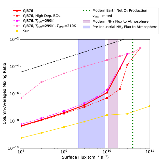
We find NH3 to enter runaway at biochemically plausible surface production fluxes for Cold Haber Worlds orbiting M dwarf stars (represented by GJ 876). Specifically, our simulations indicate NH3 to enter runaway for . For a production flux of , NH3 concentrations are 70 ppmv. For comparison, the globally averaged modern NH3 flux to Earth’s atmosphere is estimated as (Bouwman et al., 1997), and the preindustrial NH3 flux is estimated as ( lower; Zhu et al. 2015), meaning that even a modern-Earth-like biosphere emits NH3 to the atmosphere at rates within an order of magnitude of the runaway threshold for an M dwarf-hosted Cold Haber World. If NH3 were net emitted at rates comparable to the net emission of O2 on Earth ( net, Zahnle et al. 2006), e.g., as a waste product of primary energy metabolism as in the Cold Haber World scenario, then NH3 would be in the runaway regime for M dwarf worlds. This statement is robust to sensitivity tests regarding climate and wet/dry deposition of non-NH3 species. High surface deposition of non-NH3 species increases the threshold for runaway by a factor of , but does not prevent the phenomenon (Appendix B). However, high surface deposition of NH3 inhibits runaway: NH3 runaway is critically dependent on the assumption that the surface is saturated in NH3, as modern Earth’s surface is saturated in O2 (Section 4; Huang et al. 2022). Irradiation by a Sun-like UV field also suppresses runaway at the fluxes studied here, due to higher photolytic NUV irradiation. M dwarf planets are more amenable to runaway compared to G dwarf planets due to their lower NUV output, as shown previously for other gases like CH4 (Segura et al., 2005). We find metabolic ammonia production to be thermodynamically profitable over the parameter space we model here (Appendix D). Overall, the example of our biosphere suggests that NH3 production fluxes compatible with photochemical runaway on M dwarf worlds are plausible, provided the critical assumption of surface saturation is met.
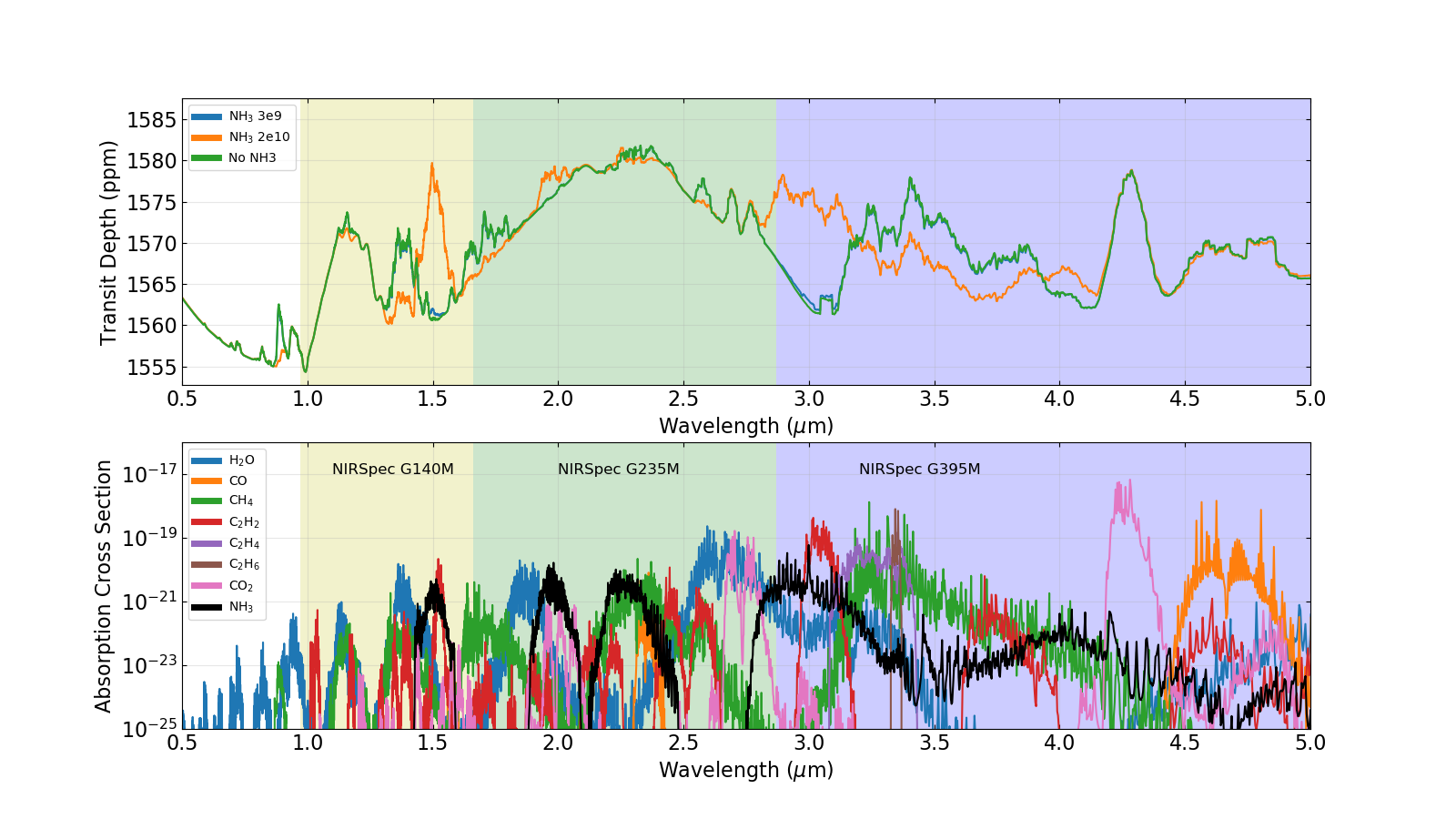
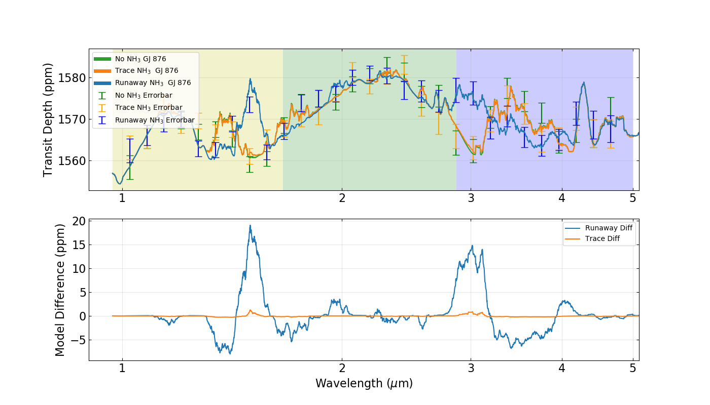
The implications of photochemical runaway for NH3 detectability are remarkable. In photochemical runaway (i.e. past a critical flux value), a mere order-of-magnitude increase in NH3 production flux translates to the difference between NH3 being essentially invisible and being highly detectable. We consider the detection of NH3 on a Cold Haber World via transmission spectroscopy with the upcoming JWST, anticipated to be the premier near-term exoplanet characterization opportunity (Cowan et al., 2015). We do not expect NH3 to be detectable at all on a 1.5 REarth exoplanet with an H2-dominated atmosphere orbiting a GJ 876-like star for a surface emission flux of , below the runaway threshold. At this surface emission flux, NH3 is confined to near the surface and rapidly decays as a function of altitude, and the marginal absorption produced by NH3 is not greater than the JWST noise floor. By comparison, 2 transits of JWST would suffice to detect the 1.45-1.55 m feature of NH3 with an average significance of for a surface emission flux of , above the runaway threshold (Figure 2, 5; Appendix B). At this surface emission flux, NH3 is in runaway. In runaway, NH3 concentrations are high and NH3 populates the upper atmosphere, leading to significantly enhanced spectral features over the non-runaway cases.
The planet scenario we have considered corresponds to a rocky, habitable planet with an H2-dominated atmosphere, for which life would have a strong metabolic incentive to produce NH3. Such planets have no analog in the solar system, and it is not known whether they exist. Terrestrial-mass planets overlaid by H2-dominated atmospheres are predicted for second-generation planets orbiting white-dwarf stars (Lin et al., 2022) and are allowed by theory for main-sequence stars depending on extreme-UV irradiation level (Owen et al., 2020). Habitable (but not rocky) planets overlaid by H2-dominated atmospheres have been proposed based on exoplanet mass/radius measurements (Madhusudhan et al., 2021), and H2-dominated atmospheres are experimentally demonstrated to be compatible with life (Seager et al., 2020). However, the main motivation for considering planets with H2-dominated atmospheres is observational: such planets are the only habitable worlds whose atmospheres will be generally accessible to spectral characterization over the next one to two decades, due to their light (therefore extended) atmospheres. Even if rocky planets with H2-dominated atmospheres do not exist, planets with H2-rich atmospheres are thermodynamically capable of supporting Cold Haber Worlds. For Cold Haber Worlds that do not feature H2-dominated atmospheres, runaway would still occur, but NH3 detection would require next-generation telescopes with a noise floor lower than JWST, a host star smaller and closer than GJ876 like TRAPPIST-1, or both (Huang et al., 2022).
We reiterate that our intent is not to singularly emphasize NH3 as a biosignature gas, but rather to use it as a case study for illustrating photochemical runaway and its implications for the detectability of trace atmospheric gases. Indeed, NH3 is just one of a steadily growing list of biogenic gases that can undergo runaway (Schwieterman et al., 2019; Sousa-Silva et al., 2020; Zhan et al., 2021). Because the phenomenon of runaway rests on the general observation that a gas’s atmospheric sinks are finite, we expect a broad range of gases in diverse habitable planetary scenarios to undergo runaway if emitted at sufficiently high fluxes, as shown in Appendix C. Specific pathological cases in which runaway fails can be identified with detailed photochemical measurements and modeling (Appendix E). Abiotic production can also drive runaways (e.g., impacts may lead to CO runaway; (Kasting, 1990)); therefore, abiotic false-positive analyses remain essential for biosignature gases, in or out of runaway.
4 Discussion
Photochemical runaway lifts the photochemical control on biosignature gas accumulation. Photochemical processes like photolysis are predicted to limit the concentrations of most gaseous products of biology to undetectable levels on habitable planets (Domagal-Goldman et al., 2011; Kasting et al., 2014; Sousa-Silva et al., 2020; Zhan et al., 2021). However, in the runaway phase, this control is lifted, making possible much higher, potentially detectable concentrations of biosignature gases. For example, the biosignature gases PH3 and isoprene are challenging-to-impossible to detect on habitable planets with JWST unless they enter a runaway phase (Sousa-Silva et al., 2020; Zhan et al., 2021).
Researchers disagree on whether photochemical runaways are physically realistic. While photochemical runaways arise in a range of models, some researchers postulate runaways to be unphysical, and set model boundary conditions that prevent them from occurring. For example, Segura et al. (2005) argue that CH4 runaway on a modern Earth-like planet is implausible because the high pCH4 and temperature associated with CH4 runaway should thermodynamically inhibit methanogenesis, which other workers extend into a general dismissal of runaway (Rugheimer et al., 2015; Rugheimer & Kaltenegger, 2018). However, this objection is specific to planets similar to the modern Earth. On planets analogous to early Earth (i.e. with high pCO2 and pH2), methanogenesis is thermodynamically compatible with runaway (Appendix D). Furthermore, biology may produce a gas even if it is not metabolically profitable to do so, if that production meets other biological needs. For example, terrestrial biology produces abundant isoprene at considerable energetic cost, because isoprene accomplishes important secondary functions (e.g., stress mitigation; Zhan et al. 2021). Finally, modelling of the rise of O2 on Earth suggests that O2, too, underwent runaway, i.e. rapidly and nonlinearly increasing in concentration as a function of surface flux (Gregory et al. 2021; Appendix C). We therefore argue that the rise of O2 on Earth represents an actualized example of photochemical runaway, affirming its physicality.
Efficient surface deposition (e.g., via biogeochemistry) may prevent biogenic gases from becoming detectable even if they are otherwise able to enter photochemical runaway, but the example of terrestrial O2 suggests that even this barrier can be overcome. Uptake by the surface can limit the concentrations of atmospheric gases. For example, if its surface deposition is efficient, NH3 is restricted to undetectably low concentrations (Huang et al., 2022). Surface deposition can be inefficient; for example, the surface deposition of CO is inefficient due to its insolubility, and CO may enter runaway on M dwarf ocean worlds even if it is deposited at the maximum possible velocity (Kharecha et al., 2005; Schwieterman et al., 2019). However, more importantly and more generally, high biogenic gas production can make surface deposition inefficient by saturating the surface. This extreme scenario occurred with O2 on Earth. O2 dry deposition into the ocean can theoretically be as high as (Kharecha et al., 2005), which on its own would limit O2 to ppmv assuming a modern-Earth atmospheric pressure and net O2 production flux. Such oxygen concentrations are extremely low compared to modern oxygen levels of 21%, and indeed it has been suggested that O2 levels were low for some time after the advent of oxygenic photosynthesis. However, over time, O2 saturated its surface sinks, rendering deposition inefficient and permitting further O2 accumulation (Lyons et al., 2014; Daines et al., 2017). We can gain a sense of just how inefficient O2 surface deposition has become by calculating the effective ”deposition velocity” required to balance the modern net O2 surface flux in modern Earth’s 21% O2 atmosphere: , 4 orders of magnitude below the theoretical upper limit. Sustained high production of O2 has saturated O2’s surface biogeochemical sink, rendering it inefficient and permitting O2 accumulation. This is the scenario invoked in for NH3 in the Cold Haber World simulated here. We cannot expect this to happen with every biogenic gas: O2’s modest solubility facilitates saturation, and even so its complete domination of the surface-atmosphere system is limited to the last 0.5-1 Ga (Lyons et al., 2014). However, the possibility that other gases can also saturate their surface sinks and hence suppress their surface deposition rates is not implausible.
Photochemical runaway requires high but biochemically plausible production fluxes, comparable to net O2 production on Earth ( net, Zahnle et al. 2006). The magnitude of O2 production is much higher (Gebauer et al., 2017), but most of this O2 is consumed either directly or indirectly by biology; the value we utilize corresponds to production net of these biogenic sinks, as measured by reductant burial and oxidative weathering (Jacob, 1999; Catling & Kasting, 2017). It is challenging to predict from first principles which gases are likely to be produced at such high fluxes in exo-biospheres. Even on modern Earth, biogenic gas production is contingent on evolutionary history, and hard to predict from first principles. For example, isoprene is a major product of terrestrial biology, with production rates rivaling those of simple gases associated with primary metabolism (e.g., CH4), despite the fact that isoprene synthesis expends energy and fixed carbon. Rather, isoprene appears to fulfill secondary roles in terrestrial biology, such as stress mitigation. Despite isoprene’s high energetic cost of synthesis, terrestrial production of isoprene is nevertheless high enough to be near the photochemical runaway threshold on planets orbiting M dwarf stars (Zhan et al., 2021). The example of isoprene illustrates the challenge of trying to predict a gas’s production from first principles; we argue it is more observationally relevant to be aware of the possibility of diverse biogenic absorbers in exo-atmospheres.
In summary, biogenic gases produced at high but not unrealistic production fluxes can experience nonlinear increases in concentration via the phenomenon of photochemical runaway. Through this phenomenon, even photochemically reactive biosignature gases may accumulate to detectable concentrations, dramatically expanding the palette of potential molecular indicators of life’s presence. Photochemical runaway occurred for O2 on Earth; it may occur for other gases on other worlds. Runaways are especially likely on planets orbiting cool stars with low UV output like M dwarfs or white dwarfs. Excitingly, photochemical runaway implies that a world need not develop oxygenic photosynthesis or even terrestrial-type biology in order to have a biosphere that can be remotely detected. Exoplanets to date have proved to be physically more diverse than the worlds of our own solar system; their biologies and their concomitant biosignatures may prove to be similarly diverse (Seager & Bains, 2015).
Appendix A Detailed Model Inputs
In this section, we present more details regarding the model inputs used in our study.
A.1 Stellar Spectra
Figure 3 shows the stellar spectra used as inputs in our photochemical model. They are formulated as described in Section 2.1.2, and shown scaled to the modern solar constant (1 AU equivalent).
A.2 GJ 876 Stellar Parameters
We draw stellar parameters for GJ876 (Table 2) from the TESS Input Catalog (Stassun et al., 2019) and from Correia et al. (2010). These parameters are used in the simulated JWST observation of the Cold Haber World orbiting GJ 876 (Section 2.2). To match our assumptions of a planetary instellation equivalent to that received at 1.6 AU orbiting the sun, we assign a planetary semimajor axis of , in turn implying a period of days, an orbital velocity of m/s, and a transit duration of hours. Here, we have assumed a circular orbit with an impact parameter of zero (negligible orbital inclination). Assuming an impact parameter of zero maximizes the time in transit, meaning that our calculations represent a best-case scenario for number of transits required to detect the trace gas species.
| Parameter | Value |
|---|---|
| , Mass () | 0.34 |
| , Radius () | 0.35 |
| , Luminosity () | 0.0128 |
| Effective Temperature (K) | 3271 |
| Surface Gravity (, cgs) | 4.87 |
| -band Magnitude | 5.934 |
| Metallicity (dex) | 0.05 |
Note. — Stellar parameters correspond to GJ 876, and are except for metallicity, are drawn from the TESS Input Catalog (TIC) (version 8.1, accessed 08/11/2021, https://exofop.ipac.caltech.edu/tess/target.php?id=188580272; Stassun et al. 2019). Metallicity is drawn from Correia et al. (2010).
A.3 Chemical Boundary Conditions
Table 3 presents the detailed chemical boundary conditions used in our baseline simulations of NH3 runaway in an H2-N2 atmosphere. For all species, we assign either a fixed surface mixing ratio or a surface flux. The only species assigned surface mixing ratios are the major atmospheric constituents CO2, N2, and H2, depending on the planet scenario, and H2O, set based on surface temperature and an assumed relative humidity following Hu et al. (2012). For species with a surface flux, the species is assumed to be injected at the bottommost layer in the atmosphere.
| Speciesaa“X”: the full continuity-diffusion equation is solved for the species; “A”: aerosol, settles out of the atmosphere; “C”: chemically inert. Our code also has the capability to designate species as type“F”, i.e. treated as being in photochemical equilibrium (Hu et al., 2012). However, we do not consider any type “F” species in this work to better enforce mass balance (James & Hu, 2018). | Type | bbEscape flux from the TOA; a negative number corresponds to inflow. | ccSurface mixing ratio relative to dry air | ddSurface emission flux | eeDry deposition velocity, standard case | ffDry deposition velocity, high-deposition sensitivity test | Choice Notes |
|---|---|---|---|---|---|---|---|
| (cm-2 s-1) | (cm-2 s-1) | (cm s-1) | (cm s-1) | ||||
| N2 | C | 0 | 0.1 | – | – | – | |
| CO2 | X | 0 | – | Hu et al. (2012) | |||
| H2 | X | Diff.-limit. | 0.9 | – | – | – | |
| NO | X | 0 | – | 0 | 0.02 | : Harman et al. (2015). : Hu et al. (2012); Seinfeld & Pandis (2016) (Earth continent) | |
| CO | X | 0 | – | 0 | : Kharecha et al. (2005); Hu et al. (2012) (abiotic ocean). : 0.03 Hu et al. (2012); Seinfeld & Pandis (2016) (Earth continent) | ||
| O2 | X | 0 | – | 0 | 0 | : Hu et al. (2012) (no surface sink). :Domagal-Goldman et al. (2011); Harman et al. (2015) (oceanic piston velocity-limited) | |
| CH4 | X | 0 | – | 0 | : Hu et al. (2012); Harman et al. (2015) (no surface sink). : Hu et al. (2012) (Earthlike) | ||
| NH3 | X | 0 | – | variable | Prescribed (c.f. Section 2.1.4) | ||
| H | X | Diff.-limit. | – | 0 | 1 | 1 | Hu et al. (2012); Harman et al. (2015) |
| O | X | 0 | – | 0 | 1 | 1 | Hu et al. (2012); Harman et al. (2015) |
| O(1D) | X | 0 | – | 0 | 0 | 1 | : Hu et al. (2012); Harman et al. (2015)ggSpecies treated as being in photochemical equilibrium have an implicit 0 deposition velocity (abiotic). : Hu et al. (2012) (Earthlike) |
| O3 | X | 0 | – | 0 | 0.4 | 0.4 | Hu et al. (2012) |
| OH | X | 0 | – | 0 | 1 | 1 | Hu et al. (2012) |
| HO2 | X | 0 | – | 0 | 1 | 1 | Hu et al. (2012) |
| H2O | X | 0 | 0.01 | – | – | – | Hu et al. (2012) |
| H2O2 | X | 0 | – | 0 | 0.5 | 0.5 | Hu et al. (2012) |
| CH2O | X | 0 | – | 0 | 0.1 | 0.2 | :Hu et al. (2012). :Domagal-Goldman et al. (2011) |
| CHO | X | 0 | – | 0 | 0.1 | 1 | : Hu et al. (2012).:Domagal-Goldman et al. (2011) |
| C | X | 0 | – | 0 | 0 | 0 | Hu et al. (2012) |
| CH | X | 0 | – | 0 | 0 | 0 | Hu et al. (2012) |
| CH2 | X | 0 | – | 0 | 0 | 0 | Hu et al. (2012) |
| CH | X | 0 | – | 0 | 0 | 0 | Hu et al. (2012) |
| CH3 | X | 0 | – | 0 | 0 | 1 | :Hu et al. (2012). :Domagal-Goldman et al. (2011) |
| CH3O | X | 0 | – | 0 | 0.1 | 0.1 | Hu et al. (2012) |
| CH4O | X | 0 | – | 0 | 0.1 | 0.1 | Hu et al. (2012) |
| CHO2 | X | 0 | – | 0 | 0.1 | 0.1 | Hu et al. (2012) |
| CH2O2 | X | 0 | – | 0 | 0.1 | 0.5 | :Hu et al. (2012) (abiotic). : Hu et al. (2012) (Earthlike) |
| CH3O2 | X | 0 | – | 0 | 0.1 | 1 | :Hu et al. (2012) (abiotic). : Hu et al. (2012) (Earthlike) |
| CH4O2 | X | 0 | – | 0 | 0.1 | 0.1 | Hu et al. (2012) |
| C2 | X | 0 | – | 0 | 0 | 0 | Hu et al. (2012) |
| C2H | X | 0 | – | 0 | 0 | 0 | Hu et al. (2012) |
| C2H2 | X | 0 | – | 0 | 0 | 0 | Hu et al. (2012) |
| C2H3 | X | 0 | – | 0 | 0 | 0 | Hu et al. (2012) |
| C2H4 | X | 0 | – | 0 | 0 | 0 | Hu et al. (2012) |
| C2H5 | X | 0 | – | 0 | 0 | 0 | Hu et al. (2012) |
| C2H6 | X | 0 | – | 0 | Hu et al. (2012) | ||
| C2HO | X | 0 | – | 0 | 0.1 | 0.1 | Hu et al. (2012) |
| C2H2O | X | 0 | – | 0 | 0.1 | 0.1 | Hu et al. (2012) |
| C2H3O | X | 0 | – | 0 | 0.1 | 0.1 | Hu et al. (2012) |
| C2H4O | X | 0 | – | 0 | 0.1 | 0.1 | Hu et al. (2012) |
| C2H5O | X | 0 | – | 0 | 0.1 | 0.1 | Hu et al. (2012) |
| S | X | 0 | – | 0 | 0 | 1 | :Hu et al. (2012). :Domagal-Goldman et al. (2011) |
| S2 | X | 0 | – | 0 | 0 | 0 | Hu et al. (2012) |
| S3 | X | 0 | – | 0 | 0 | 0 | Hu et al. (2012) |
| S4 | X | 0 | – | 0 | 0 | 0 | Hu et al. (2012) |
| SO | X | 0 | – | 0 | 0 | Hu et al. (2012); Domagal-Goldman et al. (2011) | |
| SO2 | X | 0 | – | 1 | 1 | Hu et al. (2012) | |
| SO | X | 0 | – | 0 | 0 | 1 | :Hu et al. (2012) (abiotic). : Hu et al. (2012) (Earthlike) |
| SO | X | 0 | – | 0 | 0 | 1 | :Hu et al. (2012) (abiotic). : Hu et al. (2012) (Earthlike) |
| SO3 | X | 0 | – | 0 | 1 | 1 | Hu et al. (2012) |
| H2S | X | 0 | – | 0.015 | 0.015 | Hu et al. (2012) | |
| HS | X | 0 | – | 0 | 0 | 1 | :Hu et al. (2012). :Domagal-Goldman et al. (2011) |
| HSO | X | 0 | – | 0 | 0 | 1 | :Hu et al. (2012). :Domagal-Goldman et al. (2011) |
| HSO2 | X | 0 | – | 0 | 0 | 0.1 | :Hu et al. (2012) (abiotic). : Hu et al. (2012) (Earthlike) |
| HSO3 | X | 0 | – | 0 | 0.1 | 0.1 | Hu et al. (2012) |
| H2SO4 | X | 0 | – | 0 | 1 | 1 | Hu et al. (2012) |
| H2SO4(A) | A | 0 | – | 0 | 0.2 | 0.2 | Hu et al. (2012) |
| S8 | X | 0 | – | 0 | 0 | 0.2 | :Hu et al. (2012) (abiotic). : Hu et al. (2012) (Earthlike) |
| S8(A) | A | 0 | – | 0 | 0.2 | 0.2 | Hu et al. (2012) |
| OCS | X | 0 | – | 0 | 0.01 | 0.01 | Hu et al. (2012) (Earthlike) |
| CS | X | 0 | – | 0 | 0 | :Hu et al. (2012). :Domagal-Goldman et al. (2011) | |
| CH3S | X | 0 | – | 0 | 0.01 | 0.01 | Hu et al. (2012) |
| CH4S | X | 0 | – | 0 | 0.01 | 0.01 | Hu et al. (2012) |
| N | X | 0 | – | 0 | 0 | 0 | Hu et al. (2012) |
| NH2 | X | 0 | – | 0 | 0 | 1 | :Hu et al. (2012). :Domagal-Goldman et al. (2011) |
| NH | X | 0 | – | 0 | 0 | 0 | Hu et al. (2012) |
| N2O | X | 0 | – | 0 | 0 | 0 | Hu et al. (2012); Hu & Diaz (2019) |
| NO2 | X | 0 | – | 0 | 0.02 | :Domagal-Goldman et al. (2011). :Hu et al. (2012) | |
| NO3 | X | 0 | – | 0 | 1 | 1 | Hu et al. (2012) |
| N2O5 | X | 0 | – | 0 | 1 | 4 | :Hu et al. (2012); Hu & Diaz (2019) (abiotic). : Hu et al. (2012) (Earthlike) |
| HNO | X | 0 | – | 0 | 0 | 1 | :Hu et al. (2012). :Domagal-Goldman et al. (2011) |
| HNO2 | X | 0 | – | 0 | 0.5 | 0.5 | Hu et al. (2012) |
| HNO3 | X | 0 | – | 0 | 1 | 4 | :Hu et al. (2012); Hu & Diaz (2019) (abiotic). : Hu et al. (2012) (Earthlike) |
| HNO4 | X | 0 | – | 0 | 1 | 4 | :Hu et al. (2012); Hu & Diaz (2019) (abiotic). : Hu et al. (2012) (Earthlike) |
| HCN | X | 0 | – | 0 | 0.01 | :Tian et al. (2011). :Hu et al. (2012) | |
| CN | X | 0 | – | 0 | 0.01 | 1 | :Hu et al. (2012). :Tian et al. (2011) |
| CNO | X | 0 | – | 0 | 0 | 1 | :Hu et al. (2012). :Tian et al. (2011) |
| HCNO | X | 0 | – | 0 | 0 | 1 | :Hu et al. (2012). :Tian et al. (2011) |
| CH3NO2 | X | 0 | – | 0 | 0.01 | 0.01 | Hu et al. (2012) |
| CH3NO3 | X | 0 | – | 0 | 0.01 | 0.01 | Hu et al. (2012) |
| CH5N | X | 0 | – | 0 | 0 | 1.0 | :Hu et al. (2012). : assigned as 1 based on solubility (c.f. Hu et al. (2012)) |
| C2H2N | X | 0 | – | 0 | 0 | 0.02 | :Hu et al. (2012). : assigned as 0.02 as a reactive radical following Hu et al. (2012) |
| N2H2 | X | 0 | – | 0 | 0 | 1 | :Hu et al. (2012). : assigned as 1 following N2H4 (below) |
| N2H3 | X | 0 | – | 0 | 0 | 1 | Hu et al. (2012). :Domagal-Goldman et al. (2011) |
| N2H4 | X | 0 | – | 0 | 0 | 1 | :Hu et al. (2012). : assigned as 1 based on solubility (c.f. Hu et al. (2012)) |
Note. — For the bottom boundary condition, either the surface mixing ratio or the surface flux and deposition velocity are specified.
Appendix B NH3 Photochemical Runaway in Detail
We discuss here the runaway of NH3 in the Cold Haber World scenario in more detail, including sensitivity tests. NH3 runaway has not been previously reported in the literature. The solubility of NH3 means that in most terrestrial planet contexts, wet deposition (rainout) will regulate pNH3 and photochemistry is largely irrelevant (Huang et al., 2022). However, if the surface can be saturated in NH3, e.g. due to a biosphere that is a net source of NH3 as invoked in the Cold Haber World scenario we simulate, then photochemistry controls pNH3 (Kasting, 1982; Seager et al., 2013a, b). In this case, we find the main NH3 loss mechanism to be direct photolysis, as found by Kuhn & Atreya (1979) and Kasting (1982) for N2-dominated atmospheres (early Earth). We found photolysis to dominate other photochemical loss processes by orders of magnitude. Due to the generally lower UV output of M dwarfs at the NH3-photolyzing nm wavelengths, NH3 enters runaway and becomes detectable for M dwarfs at fluxes for which it is still firmly photochemically limited to undetectable concentrations for solar-type stars.
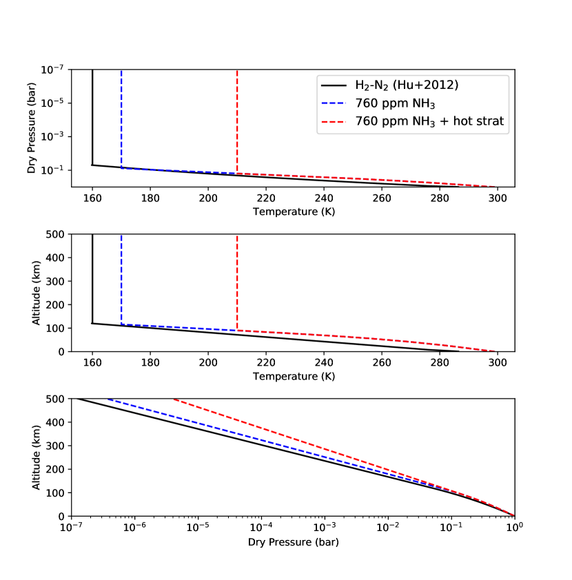
We considered the impact of NH3 greenhouse warming on NH3 runaway. For the H2-dominated Cold Haber World planetary scenario we study here, we found the greenhouse warming due to NH3 to be relatively modest, because NH3 absorption near the peak of the planet’s outgoing longwave radiation (OLR) occurs at similar wavelengths as the strong H2-H2 collision-induced absorption (CIA) in our H2-dominated scenario. Specifically, we found that adding 55 ppmv NH3 (corresponding approximately to the 70 ppmv predicted in our base case calculations for cm-2 s-1) increased the surface temperature by only 11K, from 288K to 299K. At this abundance, NH3 is already detectable with an average significance of in 2 transits from JWST. We constructed a new temperature-pressure profile evolving as a wet adiabat from K to an isothermal stratosphere of K (Figure 4), and reran our simulations, adjusting our surface H2O molar mixing ratio boundary condition from 0.01 to 0.02 to account for higher H2O saturation pressure. We found a negligible impact of higher surface temperature on NH3 accumulation. Note that the main effect of higher is to increase the water vapor content, and hence H and OH production rates, in the lower atmosphere. As the main photochemical sink of NH3 is direct photolysis at higher altitudes, NH3 accumulation is not strongly affected by changes in lower-atmosphere H2O abundance.
We considered the possibility of higher stratospheric temperatures, and their potential effect on NH3 accumulation. NH3 and its photochemical product N2H4 are strong UV absorbers, and we considered the possibility that their absorption of UV might warm the stratosphere, as does O3 on Earth. To conduct a sensitivity test for this possibility, we constructed a temperature-pressure profile evolving as a wet adiabat from K to an isothermal stratosphere of K (Figure 4), and reran our simulations, adjusting our surface H2O mixing ratio boundary condition from 0.01 to 0.02 to account for higher H2O saturation pressure. We chose K based on modern Earth’s empirical tropopause temperature, which is significantly warmer than the implied by our climate calculations and thus should provide a conservative upper bound. We found that warmer stratospheres lead to much higher NH3 abundances for the same , i.e. warmer stratospheres promoted the accumulation of NH3. We attribute this to the stabilization of NH3 due to higher production of H driven by higher stratospheric H2O abundances. In more detail: Hu et al. (2012) report the main source of H in the atmospheres of habitable worlds with H2-N2 atmospheres to be H2O photolysis, via
| (B1) | |||
| (B2) |
Therefore, increasing stratospheric H2O increases H production. Kasting (1982) reports that increased H stabilizes NH3 by aiding the recombination ; we observe the same. Kasting (1982) also indicated that the removal of N2H3 stabilizes NH3, since N2H3 is the key intermediary en route from NH3 to N2. Higher H suppresses N2H3 via , stabilizing NH3. H also suppresses N2H2 and N2H4, which are other intermediaries in the oxidation of NH3 to N2. Therefore, our finding that hotter stratospheres stabilize NH3 is consistent with past work. Indeed, we observed higher NH3 and lower NH2, N2H2, NH2H3, and N2H4 in our ”hot stratosphere” simulations compared to our standard simulations, as expected by this theory.
At high NH3 concentrations, our model predicts elevated concentrations of N2H4 (hydrazine), which is condensable at habitable temperatures. This raises the possibility of hydrazine haze in high-NH3 atmospheres. We compared the hydrazine concentrations predicted by our model to the saturation pressure of hydrazine in equilibrium with the solid phase, using the expression of Atreya et al. (1977). We found hydrazine to be condensable in the upper atmosphere if the stratosphere is cold ( K), but not if the stratosphere is warm ( K). This is both because the condensation pressure of N2H4 is higher at higher temperatures, and because warmer stratospheres inhibit N2H4 accumulation, as above. Since the high NH3 abundances that may produce condensable N2H4 should also produce warmer stratospheric temperatures (see Rugheimer & Kaltenegger 2018 for CH4), it is unclear whether haze should in fact form in high-NH3 atmospheres; coupled climate-photochemistry calculations are required to resolve this ambiguity. If N2H4 haze does form, then it might inhibit detection of spectral features of NH3 and other molecules in transmission spectra, as has been observed in large gaseous exoplanet atmospheres (Deming & Seager, 2017). On the other hand, N2H4 ice has spectral features that may enable its unique identification, in which case N2H4 haze could be used as a probe of NH3, comparable to the way in which organic haze has been suggested as a probe of organic gas production (Zheng et al., 2008; Arney et al., 2018).
We now turn to the effect of photochemical runaway on the detectability of NH3. We compare simulated observations of our 1.5 , 5 Cold Haber World with cm-2 s-1, cm-2 s-1 (not in NH3 runaway), and cm-2 (NH3 runaway) binned to in Figure 5. The cm-2 s-1 simulated observation cannot be differentiated from the cm-2 s-1 observation with JWST; the JWST noise floor exceeds the difference between the models. On the other hand, the cm-2 s-1 simulated observation can be be differentiated from the cm-2 s-1 simulated observation with two JWST transits. Specifically, in a suite of 100 simulated observations444The simulation parameters are identical; the simulations differ only in their randomly generated noise. of two transits of our planetary scenario with JWST, the m NH3 feature can be distinguished with an average significance of . The m NH3 feature is not robustly detected with two transits (average significance ), and requires additional transit observations.
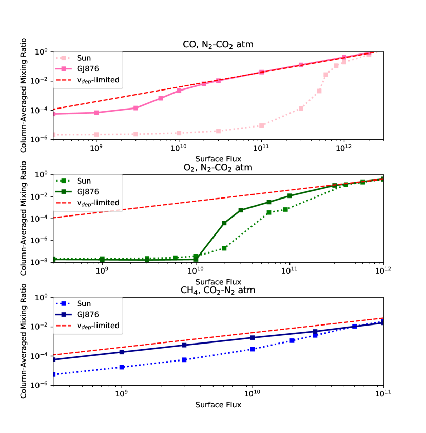
Appendix C Photochemical Runaway of CO, O2, and CH4
We illustrate the generality of the phenomenon of runaway by calculating the concentration as a function of surface production flux for three gases other than NH3 using our photochemical model (see Tables 4, 5). We consider the accumulation of CH4 in a CO2-dominated atmosphere and the accumulation of CO and O2 in N2-dominated atmospheres, for both solar and M dwarf irradiation (represented by GJ 876), to complement our earlier simulation of NH3 accumulation in an H2-dominated atmosphere. We chose these gases because they are well studied in the literature, meaning that their reaction networks are relatively complete, and because runaway of these gases has been studied in previous work (albeit not as a unified concept) (Kasting, 1990; Pavlov et al., 2003; Segura et al., 2005; Zahnle et al., 2006; Schwieterman et al., 2019; Gregory et al., 2021). We made these choices to demonstrate that the phenomenon of runaway is not necessarily attributable to incomplete reaction networks, nor is it unique to our model. We similarly chose background atmospheres of varying redox state to illustrate the generality of the phenomenon. Unless otherwise stated, we used the same model choices as for NH3 runaway, to illustrate the recovery of the runaway phenomenon for diverse gases with a uniform model calculation.
C.1 Methods
To demonstrate the generality of runaway, we model the runaway of CO, O2, and CH4 in N2- or CO2-dominated atmospheres. Such runaways have been reported previously in the literature, though they have not always been identified as such. To carry out these calculations, we use the same photochemical model and reaction network as for the NH3 runaway. We include a lightning-produced NO flux of cm-2 s-1 injected at the surface, and an equal conjugate CO production, for redox balance (Harman et al., 2018; Hu & Diaz, 2019). For an Earth-sized planet, these correspond to global mass fluxes of 0.8 Tg NO yr-1 and 0.8 Tg CO year-1; this is lower than modern Earth, because CO2 is a less efficient oxidant of N2 than O2 (Harman et al., 2018). We adopt vertical temperature, pressure, and eddy diffusion profiles from Hu et al. (2012), following the logic detailed therein. We follow Hu et al. (2012) in adopting semimajor axes for the N2 and CO2 atmospheres of 1.0 and 1.3 for the solar instellation case, based on crude climate calculations, and we scale our GJ 876 spectra to the same total instellation as in the corresponding Solar case for each atmospheric scenario.
For chemical boundary conditions, we modify the low deposition velocity boundary conditions given in Table 3, as indicated in Table 5. As these instances of runaway have been previously reported, we consider them robust, and do not carry out the high deposition velocity sensitivity test executed for NH3. For these CO2- and N2-dominated atmospheric scenarios, we employ the additional solution quantity check of verifying the atmospheric redox balance (Harman et al., 2015; James & Hu, 2018). We are unable to employ this quality check for the H2-dominated atmospheric scenario studied for NH3 runaway in the main paper because a fixed H2 mixing ratio boundary condition is employed in this case, and our code is incapable of calculating atmospheric redox balance when a fixed mixing ratio boundary condition is employed with a species with a non-neutral redox state.
To simulate CO runaway, we chose an atmospheric scenario motivated by early Earth, for which CO runaway has been extensively studied (Kasting, 1990, 2014; Schwieterman et al., 2019; Ranjan et al., 2020). We chose an N2-dominated atmosphere, and adopted a CO2 mixing ratio of 0.01. We selected a low CO2 mixing ratio to ensure that photolytic production of CO from CO2 photolysis did not tip the atmosphere into runaway on its own, whether orbiting a Sun-like star or an M dwarf (Kasting, 2014; Hu et al., 2020).
To simulate O2 runaway, we again chose an atmospheric scenario motivated by early Earth, which experienced O2 buildup (Gregory et al., 2021). We chose an N2-dominated atmosphere, and adopted a CO2 mixing ratio of 0.01. We selected a low CO2 mixing ratio to ensure that photolytic production of O2 did not tip the atmosphere into runaway on its own (Hu et al., 2020).
To simulate CH4 runaway, we chose a CO2-dominated atmospheric scenario, because our model is not equipped to handle the hydrocarbon haze formation that accompanies high CH4/CO2 ratios. We adopt a CO2 mixing ratio of 0.9 and an N2 mixing ratio of 0.1.
| Parameter | CO Runaway | O2 Runaway | CH4 Runaway |
|---|---|---|---|
| Bulk Composition | % N2, 1% CO2 | % N2, 1% CO2 | 90% CO2, 10% N22 |
| Surface Water Vapor Mixing Ratio | 0.01 | 0.01 | 0.01 |
| Surface Pressure (bar) | 1 | 1 | 1 |
| Surface Temperature (K) | 288 | 288 | 288 |
| Stratospheric Temperature (K) | 200 | 200 | 175 |
| Stellar Irradiation Considered | Sun, GJ 876 | Sun, GJ 876 | Sun, GJ 876 |
| Stellar Constant Relative to Modern Earth | 1 | 1 | 0.6 |
| Planet Mass () | 1 | 1 | 1 |
| Planet Radius () | 1 | 1 | 1 |
Note. — Bulk planetary properties assumed in modeling the CO, O2, and CH4 runaways. Planet scenarios are based on the N2-dominated and CO2-dominated exoplanet atmospheric benchmark scenarios of Hu et al. (2012).
| Speciesaa“X”: the full continuity-diffusion equation is solved for the species; “A”: aerosol, settles out of the atmosphere; “C”: chemically inert. Our code also has the capability to designate species as type“F,” i.e. treated as being in photochemical equilibrium (Hu et al., 2012). However, we do not consider any type “F” species in this work to better enforce mass balance (James & Hu, 2018). | Type | bbEscape flux from the TOA; a negative number corresponds to inflow. | ccSurface mixing ratio relative to dry air | ddSurface emission flux | eeDry deposition velocity, standard case | Choice Notes |
|---|---|---|---|---|---|---|
| (cm-2 s-1) | (cm-2 s-1) | (cm s-1) | ||||
| CO Runaway in N2-CO2 Atmosphere | ||||||
| N2 | C | 0 | 0.99 | – | – | |
| CO2 | X | 0 | 0.01 | – | – | |
| H2 | X | Diff.-limit. | – | 0 | Hu et al. (2012) | |
| NO | X | 0 | – | Harman et al. (2015); Hu & Diaz (2019) | ||
| CO | X | 0 | – | variable | ||
| O2 | X | 0 | – | 0 | 0 | Hu et al. (2012) |
| CH4 | X | 0 | – | 0 | Hu et al. (2012) | |
| NH3 | X | 0 | – | 0 | 0 | Harman et al. (2015) |
| O2 Runaway in N2-CO2 Atmosphere | ||||||
| N2 | C | 0 | 0.99 | – | – | |
| CO2 | X | 0 | 0.01 | – | – | |
| H2 | X | Diff.-limit. | – | 0 | Hu et al. (2012) | |
| NO | X | 0 | – | Harman et al. (2015); Hu & Diaz (2019) | ||
| CO | X | 0 | – | Kharecha et al. (2005) | ||
| O2 | X | 0 | – | variable | – | |
| CH4 | X | 0 | – | 0 | Hu et al. (2012) | |
| NH3 | X | 0 | – | 0 | 0 | Harman et al. (2015) |
| CH4 Runaway in CO2-N2 Atmosphere | ||||||
| N2 | C | 0 | 0.1 | – | – | |
| CO2 | X | 0 | 0.9 | – | – | |
| H2 | X | Diff.-limit. | – | 0 | Hu et al. (2012) | |
| NO | X | 0 | – | Harman et al. (2015); Hu & Diaz (2019) | ||
| CO | X | 0 | – | Kharecha et al. (2005); Hu et al. (2012) | ||
| O2 | X | 0 | – | 0 | 0 | Hu et al. (2012) |
| CH4 | X | 0 | – | variable | ||
| NH3 | X | 0 | – | 0 | 0 | Harman et al. (2015) |
Note. — For the bottom boundary condition, either the surface mixing ratio or the surface flux and deposition velocity are specified.
C.2 Results
In this section, we discuss our simulations of CO, O2, and CH4 runaway in the context of the literature (Figure 6). Photochemical runaway occurs for a range of gases and atmosphere types, and is not unique to our model.
CO runaway is the best understood due to its photochemical simplicity: the only significant sink of CO is reaction with OH, whose main source in anoxic atmospheres is H2O photolysis. At low , the concentration of CO, [CO], is a weak function of its surface emission flux due to the production of CO by CO2 photolysis; must exceed photolytic production to affect [CO]. If exceeds the H2O photolysis rate , CO saturates this sink and accumulates rapidly until it is limited by surface deposition (Kasting, 1990, 2014). For the temperate, ocean-bearing planetary scenario we consider, is limited by stellar NUV irradiation; consequently, CO runaway occurs at much lower fluxes on M dwarf planets due to their lower NUV irradiation and hence lower (Segura et al., 2005).
O2 runaway is also discussed in the literature, thought not by name. O2 runaway is more complex and challenging to model compared to CO runaway. At low , [O2] is a weak function of , due to strong photochemical production in the upper atmosphere from recombination of O derived from CO2 photolysis. At low , [O2] is limited by reactions with atmospheric reductants, mediated by UV photons. If exceeds the reductant flux into the atmosphere (here, primarily volcanogenic H2, cm2 s-1 O2 equivalents), O2 overcomes its photochemical sinks, and accumulates rapidly as a function of until it is limited by surface processes. This is consistent with our understanding of the processes governing the rise of O2 in Earth’s atmosphere (Goldblatt et al., 2006; Zahnle et al., 2006; Daines et al., 2017; Gregory et al., 2021). Because the main limit to O2 accumulation is reductant supply and not UV flux, it is not predicted to be significantly easier to accumulate on M dwarf planets, though this is not the case for a more reducing atmosphere (e.g., H2-dominated) where the reductant supply is not limiting.
CH4 runaway has been briefly considered in the literature (Prather, 1996; Pavlov et al., 2003; Segura et al., 2005). For planets orbiting Sun-like stars, OH is the main sink of CH4 at low . As with CO, when grows large enough to complete with , it saturates the OH supply and increases quadratically until it is limited photochemically by direct photolysis. This is consistent with the similarly quadratic growth reported by Pavlov et al. (2003). CH4 does not enter true runaway (complete removal of all photochemical constraints on buildup) over the range of CH4 emission fluxes we simulate here. For sufficiently high we expect that the direct photolysis sink would eventually saturate, but are unable to probe this regime because it would cause [CH4]/[CO2]. Our model is not valid in this regime because our model does not include hydrocarbon haze, and optically thick hydrocarbon haze formation is expected in this regime (DeWitt et al., 2009; Arney et al., 2016, 2017; Hu et al., 2012). Nevertheless, CH4 photolysis is inefficient enough that CH4 still accumulates to very high concentrations (Mount et al., 1977; Chen & Wu, 2004; Hu et al., 2012). The situation is different for the GJ 876 case. The low NUV output of our proxy M dwarf means that our CO2-dominated atmosphere destabilizes to CO and O2 (Hu et al., 2020). In this case, CH4 accumulates in an essentially OH-free atmosphere thanks to suppression by high atmospheric CO, and is controlled by photolysis and deposition at all modeled here. Hu et al. (2020) report this destabilization to be extremely sensitive to the details of the photochemical network. As a sensitivity test, we prescribed an unrealistically high cm/s, to force the atmosphere into a low-CO/O2 state. In this case, we again observed a transition from OH attack to direct photolysis as the main limit on [CH4], though OH attack remained a smaller sink than in the solar case because of the lower OH production on M dwarf planets.
Appendix D Thermodynamic Limits on Runaway
In this section, we quantitatively examine the qualitative argument of Segura et al. (2005) and Rugheimer et al. (2015) that runaway is not physical due to biological feedbacks. Specifically, Segura et al. (2005) and Rugheimer et al. (2015) argue that microbial methanogenesis would become thermodynamically ”unprofitable” at high pCH4, thereby providing a feedback loop to stabilize pCH4 by reducing CH4 production. Segura et al. (2005) and Rugheimer et al. (2015) postulate an upper limit on pCH4 of bar. By analogy Rugheimer et al. (2015) dismiss the possibility of runaway of other gases, such as N2O, and Rugheimer & Kaltenegger (2018) dismiss the possibility of runaway for early Earth as well.
We examine this argument on thermodynamic grounds using the framework of Seager et al. (2013a), who in turn implement the criteria of Hoehler (2004). We affirm the argument of Segura et al. (2005) and Rugheimer et al. (2015) that thermodynamic constraints may prevent methanogenic microbes from triggering a CH4 runaway on modern-Earth-like planets. However, high CH4 (pCH bar) remains thermodynamically compatible with methanogenesis on early-Earth-like worlds, which feature elevated concentrations of the CO2 and H2 that are the substrates of methanogenesis. We analyze the hypothetical ”ammoniagenesis” metabolism (Seager et al., 2013a, b; Bains et al., 2014), and show it to be compatible with runaway concentrations of NH3 (pNH bar). Our analysis is simple, and does not encode a full ecosystem model, e.g., Sauterey et al. (2020). However, this simplicity also reduces the terracentricity of our analysis (Seager & Bains, 2015), and we contend that it is sufficient to argue against a blanket dismissal of photochemical runaway on purely thermodynamic grounds.
D.1 Thermodynamics of Metabolic Gas Production
We follow Seager et al. (2013a) in considering thermodynamic limits on metabolic gas production.
The free energy yielded by a metabolic reaction can be calculated from thermodynamics, via
, where is the standard free energy of the reaction, is the temperature, J mol-1 K-1 is the universal gas constant, and is the reaction quotient.
can be estimated from the difference between the total standard Gibbs free energy of formation of the products and the reactants, i.e.
, where is the standard free energy of formation of species , is the stoichiometric coefficient associated with species , and the indices and count over products and reactants, respectively.
is calculated as
, where is the activity of species . We approximate our metabolic reactions as proceeding in dilute aqueous solution, permitting us to ignore salinity effects and to simplify .
For example, for methanogenesis,
| (D1) | |||
| (D2) | |||
| (D3) |
We note that is a relative quantity, and that the reference species can differ between thermodynamic databases. Therefore, it is important to use an internally consistent thermodynamic database when conducting thermodynamic calculations. We take our from Amend & Shock (2001). Further, care must be taken to use the corresponding to the phase being considered, i.e. when considering aqueous-phase a different must be used than when considering gas-phase . We do so.
We can translate into thermodynamic constraints on microbial metabolic gas production. We consider two constraints, using the terminology of Hoehler (2004):
-
1.
Biological Energy Quantum (BEQ): the Gibbs free energy liberated by metabolism () must exceed a minimum threshold to be usefully harnessed by the cell. The threshold Gibbs free energy of metabolism required to be usefully harnessed by the cell is empirically constrained for actively growing terrestrial life to be (Hoehler, 2004):
. Here, the mol-1 refers to mol of reaction, with the reaction written to minimize the number of molecules. We note this constraint to be conservative; one species identified in Hoehler (2004) could survive at , suggesting it could grow at .
-
2.
Maintenance Energy: organisms must generate energy at a minimum rate in order survive as active organisms able to grow. This minimum rate increases with temperature. For anaerobic terrestrial life, this minimum energy production rate has been empirically measured to be where the g-1 refers to grams of wet biomass (Tijhuis et al., 1993; Hoehler, 2004; Seager et al., 2013a). can be related to via , where is the production rate of the metabolic byproduct in units of mol g-1 s-1. In the studies we reviewed, mol g-1 s-1 (Müller et al., 1986; Patel et al., 1978; Patel & Roth, 1977; Pennings et al., 2000; Perski et al., 1981; Schönheit & Beimborn, 1985; Takai et al., 2008; Zinder & Koch, 1984) and we adopt this as our upper limit, providing our second constraint:
D.2 Thermodynamic Limits on Methanogenesis
We consider methanogenesis, with general reaction represented by (Bains et al., 2014):
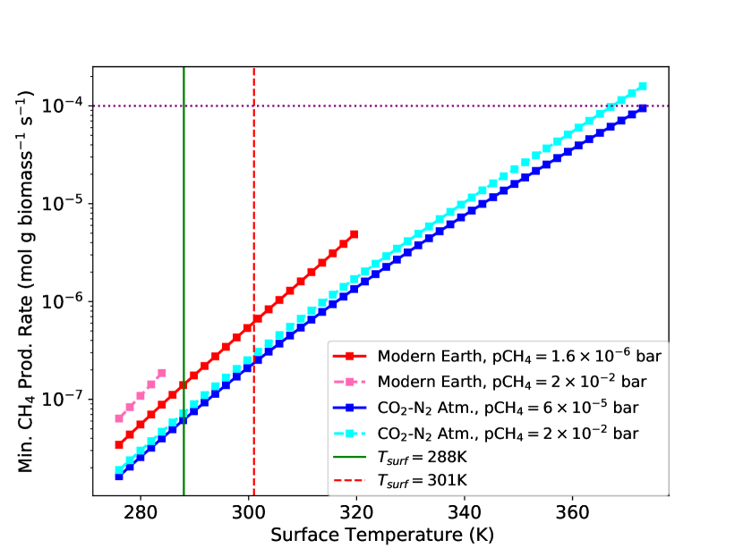
Methanogens are strict anaerobes. Consequently, on oxic modern Earth, methanogens are confined to anaerobic environments, with [CO2] present at mM concentrations and [H2] present at nM concentrations (Megonigal et al., 2014). We calculate the at which methanogenesis satisfies the criteria in Section D.1 for [CO2]=3 mM, [H2]=3 nM, and pCH bar and bar, corresponding to modern Earth and an Earth in CH4 runaway, respectively (Figure 7). \textFor modern Earth in CH4 runaway, we find that methanogenesis is only profitable for K. For comparison, we calculate K for this planetary scenario, affirming the argument of Segura et al. (2005) and Rugheimer et al. (2015) that thermodynamic feedbacks may inhibit CH4 runaway on a modern-Earth-like planet. However, methanogenesis would be allowed if [CO2] or [H2] were higher (e.g., 9 mM, 9 nM), rather than the intermediate values (3 nM, 3 nM) we have chosen here; consequently, we cannot fully rule out the possibility of CH4 runaway on modern Earth-like planets.
On the other hand, planets more similar to early Earth, i.e. anoxic, with CO2-N2 atmospheres, are more thermodynamically favorable for methanogenesis. We simulate such a planet in Appendix C, which features pCO2=0.9 bar, pH bar, and pCH4= and pCH4=, corresponding to cm-2s-1 and cm-2s-1, respectively. Using the climate model described in Section 2.3, we predict surface warming of K corresponding to this CH4 inventory, relative to a base climate with K. Methanogenesis remains profitable up to very high temperatures for an early Earth-like world, including the K (vertical red dashed line) expected in CH4 runaway.
Note that for the modern Earth case, we considered [CO2] and [H2], whereas for the early Earth-like case, we considered pCO2 and pH2. For these calculations, we have been careful to use from Amend & Shock (2001) corresponding to the aqueous phase and gas phase, respectively.
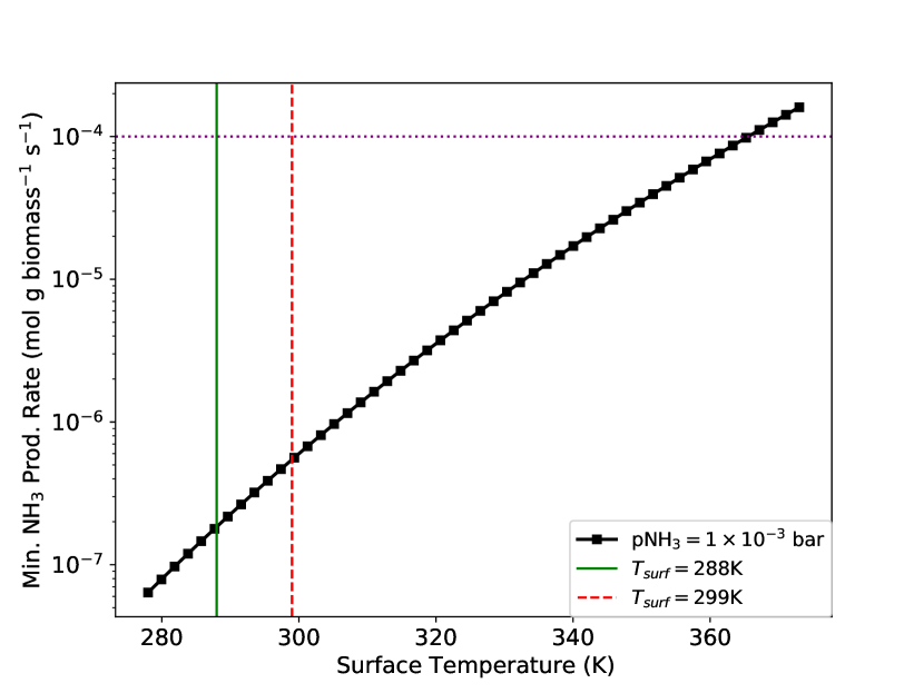
D.3 Thermodynamic Limits on Ammonia Production in Cold Haber World Scenario
We consider the hypothetical ”ammoniagenesis” metabolism proposed for Cold Haber Worlds and modeled in this paper, with the general reaction (Seager et al., 2013a, b; Bains et al., 2014)
For the atmospheric scenario we simulate in this paper, pH2=0.9 bar, pN2=0.1 bar, and pNH3=0.001 bar in runaway. For these parameters, the ammoniagenesis is profitable for K (Fig. 8). For comparison, we predict K for pNH bar. We conclude that ammoniagenesis remains profitable in NH3 runaway, based on the criteria from Hoehler (2004).
We further considered whether an H2-dominated atmosphere is required for the Cold Haber World. We reran the calculation above for pN2=0.1 bar and pH2=0.01 bar, and found that ammoniagenesis remains thermodynamically profitable across a wide range of habitable temperatures. Early Earth-like planets are predicted to host H2 mixing ratios of up to 10% if H2 escape is below the diffusion limit, due to, e.g., cooling of the upper atmosphere by high CO2 abundances (Tian et al., 2005; Liggins et al., 2020). This implies that even an early Earth-like planet with a non-H2 dominated atmosphere would be thermodynamically compatible with ammoniagenesis, though the metabolic incentive to develop this metabolism would be proportionately reduced.
Appendix E Failure Modes for Photochemical Runaway
In this section, we consider pathological scenarios in which gases might fail to enter photochemical runaway despite high production flux.
The key requirement for photochemical runaway is that the radical production in the atmosphere vary sublinearly with the runaway gas flux, so that the runaway gas can saturate its photochemical sinks. One scenario in which this condition fails corresponds to combustion-explosion conditions. In conditions of sufficiently extreme disequilibrium (e.g., the coexistence of sufficiently-abundant H2 and O2), chain propagation reactions (radicals tend to make more radicals) can dominate over chain termination reactions (radicals tend to make nonradicals). In such conditions, energetic events can trigger runaway increase in radical concentrations until the substrates are exhausted. This condition can be checked by comparing to experimental combustion-explosion studies (Grenfell et al., 2018).
More generally, there may exist cases in which a biosignature gas self-limits its concentrations, e.g. through self-reaction or through the production of UV sensitizer. Photochemical models can check for this possibility, but careful study is required. For example, O2 does produce a UV sensitizer in the form of O3, but far from catalyzing its destruction, O3 photochemically shields O2 (Zahnle et al., 2006). Detailed photochemical networks are not available for many potential biosignature gases; the measurement of these photochemical data and their incorporation into photochemical models is required to explore the potential of novel biosignature gases for runaway.
References
- Amend & Shock (2001) Amend, J. P., & Shock, E. L. 2001, FEMS microbiology reviews, 25, 175
- Arney et al. (2018) Arney, G., Domagal-Goldman, S. D., & Meadows, V. S. 2018, Astrobiology, 18, 311, doi: 10.1089/ast.2017.1666
- Arney et al. (2016) Arney, G., Domagal-Goldman, S. D., Meadows, V. S., et al. 2016, Astrobiology, 16, 873, doi: 10.1089/ast.2015.1422
- Arney et al. (2017) Arney, G. N., Meadows, V. S., Domagal-Goldman, S. D., et al. 2017, ApJ, 836, 49, doi: 10.3847/1538-4357/836/1/49
- Atreya et al. (1977) Atreya, S. K., Donahue, T. M., & Kuhn, W. R. 1977, Icarus, 31, 348, doi: 10.1016/0019-1035(77)90027-6
- Bains et al. (2014) Bains, W., Seager, S., & Zsom, A. 2014, Life, 4, 716
- Batalha et al. (2018) Batalha, N. E., Lewis, N. K., Line, M. R., Valenti, J., & Stevenson, K. 2018, ApJ, 856, L34, doi: 10.3847/2041-8213/aab896
- Batalha et al. (2017) Batalha, N. E., Mandell, A., Pontoppidan, K., et al. 2017, PASP, 129, 064501, doi: 10.1088/1538-3873/aa65b0
- Bouwman et al. (1997) Bouwman, A., Lee, D., Asman, W., et al. 1997, Global biogeochemical cycles, 11, 561
- Catling & Kasting (2017) Catling, D. C., & Kasting, J. F. 2017, Atmospheric evolution on inhabited and lifeless worlds (Cambridge University Press)
- Chen & Wu (2004) Chen, F. Z., & Wu, C. Y. R. 2004, J. Quant. Spec. Radiat. Transf., 85, 195, doi: 10.1016/S0022-4073(03)00225-5
- Cohen & Westberg (1991) Cohen, N., & Westberg, K. 1991, Journal of physical and chemical reference data, 20, 1211
- Correia et al. (2010) Correia, A. C. M., Couetdic, J., Laskar, J., et al. 2010, A&A, 511, A21, doi: 10.1051/0004-6361/200912700
- Cowan et al. (2015) Cowan, N. B., Greene, T., Angerhausen, D., et al. 2015, PASP, 127, 311, doi: 10.1086/680855
- Curdt et al. (2004) Curdt, W., Landi, E., & Feldman, U. 2004, A&A, 427, 1045, doi: 10.1051/0004-6361:20041278
- Daines et al. (2017) Daines, S. J., Mills, B. J. W., & Lenton, T. M. 2017, Nature Communications, 8, 14379, doi: 10.1038/ncomms14379
- Deming & Seager (2017) Deming, L. D., & Seager, S. 2017, Journal of Geophysical Research (Planets), 122, 53, doi: 10.1002/2016JE005155
- DeWitt et al. (2009) DeWitt, H. L., Trainer, M. G., Pavlov, A. A., et al. 2009, Astrobiology, 9, 447, doi: 10.1089/ast.2008.0289
- Domagal-Goldman et al. (2011) Domagal-Goldman, S. D., Meadows, V. S., Claire, M. W., & Kasting, J. F. 2011, Astrobiology, 11, 419, doi: 10.1089/ast.2010.0509
- Fauchez et al. (2020) Fauchez, T. J., Villanueva, G. L., Schwieterman, E. W., et al. 2020, Nature Astronomy, 4, 372, doi: 10.1038/s41550-019-0977-7
- France et al. (2016) France, K., Parke Loyd, R. O., Youngblood, A., et al. 2016, Astrophysical Journal, 820, 89, doi: 10.3847/0004-637X/820/2/89
- Gardner et al. (2006) Gardner, J. P., Mather, J. C., Clampin, M., et al. 2006, Space Sci. Rev., 123, 485, doi: 10.1007/s11214-006-8315-7
- Gebauer et al. (2017) Gebauer, S., Grenfell, J. L., Stock, J. W., et al. 2017, Astrobiology, 17, 27, doi: 10.1089/ast.2015.1384
- Goldblatt et al. (2006) Goldblatt, C., Lenton, T. M., & Watson, A. J. 2006, Nature, 443, 683, doi: 10.1038/nature05169
- Gordon et al. (2017) Gordon, I. E., Rothman, L. S., Hill, C., et al. 2017, J. Quant. Spec. Radiat. Transf., 203, 3, doi: 10.1016/j.jqsrt.2017.06.038
- Goumri et al. (1999) Goumri, A., Rocha, J.-D. R., Laakso, D., Smith, C., & Marshall, P. 1999, The Journal of Physical Chemistry A, 103, 11328
- Gregory et al. (2021) Gregory, B. S., Claire, M. W., & Rugheimer, S. 2021, Earth and Planetary Science Letters, 561, 116818, doi: 10.1016/j.epsl.2021.116818
- Grenfell et al. (2018) Grenfell, J. L., Gebauer, S., Godolt, M., et al. 2018, ApJ, 861, 38, doi: 10.3847/1538-4357/aab2a9
- Harman et al. (2018) Harman, C. E., Felton, R., Hu, R., et al. 2018, ApJ, 866, 56, doi: 10.3847/1538-4357/aadd9b
- Harman et al. (2015) Harman, C. E., Schwieterman, E. W., Schottelkotte, J. C., & Kasting, J. F. 2015, Astrophysical Journal, 812, 137, doi: 10.1088/0004-637X/812/2/137
- Hoehler (2004) Hoehler, T. 2004, Geobiology, 2, 205
- Hu & Diaz (2019) Hu, R., & Diaz, H. D. 2019, The Astrophysical Journal, 886, 126
- Hu et al. (2020) Hu, R., Peterson, L., & Wolf, E. T. 2020, ApJ, 888, 122, doi: 10.3847/1538-4357/ab5f07
- Hu et al. (2012) Hu, R., Seager, S., & Bains, W. 2012, Astrophysical Journal, 761, 166, doi: 10.1088/0004-637X/761/2/166
- Hu et al. (2013) —. 2013, Astrophysical Journal, 769, 6, doi: 10.1088/0004-637X/769/1/6
- Huang et al. (2022) Huang, J., Seager, S., Petkowski, J. J., Ranjan, S., & Zhan, Z. 2022, Astrobiology, 22, 171, doi: 10.1089/ast.2020.2358
- Jacob (1999) Jacob, D. J. 1999, Introduction to atmospheric chemistry (Princeton University Press)
- James & Hu (2018) James, T., & Hu, R. 2018, ApJ, 867, 17, doi: 10.3847/1538-4357/aae2bb
- Kaltenegger (2017) Kaltenegger, L. 2017, Annual Review of Astronomy and Astrophysics, 55, 433
- Kasting (1982) Kasting, J. F. 1982, Journal of Geophysics Research, 87, 3091, doi: 10.1029/JC087iC04p03091
- Kasting (1990) —. 1990, Origins of Life and Evolution of the Biosphere, 20, 199, doi: 10.1007/BF01808105
- Kasting (2014) Kasting, J. F. 2014, Geological Society of America Special Papers, 504, 19
- Kasting et al. (2014) Kasting, J. F., Kopparapu, R., Ramirez, R. M., & Harman, C. E. 2014, Proceedings of the National Academy of Science, 111, 12641, doi: 10.1073/pnas.1309107110
- Kawashima & Rugheimer (2019) Kawashima, Y., & Rugheimer, S. 2019, AJ, 157, 213, doi: 10.3847/1538-3881/ab14e3
- Kharecha et al. (2005) Kharecha, P., Kasting, J., & Siefert, J. 2005, Geobiology, 3, 53
- Koll & Cronin (2019) Koll, D. D. B., & Cronin, T. W. 2019, ApJ, 881, 120, doi: 10.3847/1538-4357/ab30c4
- Kozakis et al. (2020) Kozakis, T., Lin, Z., & Kaltenegger, L. 2020, ApJ, 894, L6, doi: 10.3847/2041-8213/ab6f6a
- Kuhn & Atreya (1979) Kuhn, W. R., & Atreya, S. K. 1979, Icarus, 37, 207, doi: 10.1016/0019-1035(79)90126-X
- Laufer & Fahr (2004) Laufer, A. H., & Fahr, A. 2004, Chemical reviews, 104, 2813
- Liggins et al. (2020) Liggins, P., Shorttle, O., & Rimmer, P. B. 2020, Earth and Planetary Science Letters, 550, 116546, doi: 10.1016/j.epsl.2020.116546
- Lin et al. (2022) Lin, Z., Seager, S., Ranjan, S., Kozakis, T., & Kaltenegger, L. 2022, ApJ, 925, L10, doi: 10.3847/2041-8213/ac4788
- Loyd et al. (2016) Loyd, R. O. P., France, K., Youngblood, A., et al. 2016, Astrophysical Journal, 824, 102, doi: 10.3847/0004-637X/824/2/102
- Lustig-Yaeger et al. (2019) Lustig-Yaeger, J., Meadows, V. S., & Lincowski, A. P. 2019, AJ, 158, 27, doi: 10.3847/1538-3881/ab21e0
- Lyons et al. (2014) Lyons, T. W., Reinhard, C. T., & Planavsky, N. J. 2014, Nature, 506, 307
- Madhusudhan et al. (2021) Madhusudhan, N., Piette, A. A. A., & Constantinou, S. 2021, ApJ, 918, 1, doi: 10.3847/1538-4357/abfd9c
- Meadows et al. (2018) Meadows, V. S., Reinhard, C. T., Arney, G. N., et al. 2018, Astrobiology, 18, 630
- Megonigal et al. (2014) Megonigal, J., Hines, M., & Visscher, P. 2014, in Treatise on Geochemistry (Second Edition), second edition edn., ed. H. D. Holland & K. K. Turekian (Oxford: Elsevier), 273–359, doi: https://doi.org/10.1016/B978-0-08-095975-7.00808-1
- Möller & Wagner (1984) Möller, W., & Wagner, H. G. 1984, Zeitschrift für Naturforschung A, 39, 846
- Morley et al. (2017) Morley, C. V., Kreidberg, L., Rustamkulov, Z., Robinson, T., & Fortney, J. J. 2017, ApJ, 850, 121, doi: 10.3847/1538-4357/aa927b
- Mount et al. (1977) Mount, G. H., Warden, E. S., & Moos, H. W. 1977, Astrophysical Journall, 214, L47, doi: 10.1086/182440
- Müller et al. (1986) Müller, V., Blaut, M., & Gottschalk, G. 1986, Applied and environmental microbiology, 52, 269
- Owen et al. (2020) Owen, J. E., Shaikhislamov, I. F., Lammer, H., Fossati, L., & Khodachenko, M. L. 2020, Space Sci. Rev., 216, 129, doi: 10.1007/s11214-020-00756-w
- Patel et al. (1978) Patel, G., Khan, A., & Roth, L. 1978, Journal of Applied Bacteriology, 45, 347
- Patel & Roth (1977) Patel, G., & Roth, L. 1977, Canadian journal of microbiology, 23, 893
- Pavlov et al. (2003) Pavlov, A. A., Hurtgen, M. T., Kasting, J. F., & Arthur, M. A. 2003, Geology, 31, 87, doi: 10.1130/0091-7613(2003)031<0087:MRPA>2.0.CO;2
- Pennings et al. (2000) Pennings, J. L., Vermeij, P., de Poorter, L. M., Keltjens, J. T., & Vogels, G. D. 2000, Antonie van Leeuwenhoek, 77, 281
- Perski et al. (1981) Perski, H.-J., Moll, J., & Thauer, R. K. 1981, Archives of Microbiology, 130, 319
- Phillips et al. (2021) Phillips, C. L., Wang, J., Kendrew, S., et al. 2021, ApJ, 923, 144, doi: 10.3847/1538-4357/ac29be
- Prather (1996) Prather, M. J. 1996, Geophys. Res. Lett., 23, 2597, doi: 10.1029/96GL02371
- Ranjan et al. (2020) Ranjan, S., Schwieterman, E. W., Harman, C., et al. 2020, ApJ, 896, 148, doi: 10.3847/1538-4357/ab9363
- Reinhard et al. (2017) Reinhard, C. T., Olson, S. L., Schwieterman, E. W., & Lyons, T. W. 2017, Astrobiology, 17, 287, doi: 10.1089/ast.2016.1598
- Rodler & López-Morales (2014) Rodler, F., & López-Morales, M. 2014, Astrophysical Journal, 781, 54, doi: 10.1088/0004-637X/781/1/54
- Rogers (2015) Rogers, L. A. 2015, Astrophysical Journal, 801, 41, doi: 10.1088/0004-637X/801/1/41
- Rugheimer & Kaltenegger (2018) Rugheimer, S., & Kaltenegger, L. 2018, The Astrophysical Journal, 854, 19
- Rugheimer et al. (2015) Rugheimer, S., Kaltenegger, L., Segura, A., Linsky, J., & Mohanty, S. 2015, The Astrophysical Journal, 809, 57
- Sauterey et al. (2020) Sauterey, B., Charnay, B., Affholder, A., Mazevet, S., & Ferrière, R. 2020, Nature Communications, 11, 2705, doi: 10.1038/s41467-020-16374-7
- Schönheit & Beimborn (1985) Schönheit, P., & Beimborn, D. B. 1985, European journal of biochemistry, 148, 545
- Schwieterman et al. (2019) Schwieterman, E. W., Reinhard, C. T., Olson, S. L., et al. 2019, ApJ, 874, 9, doi: 10.3847/1538-4357/ab05e1
- Seager & Bains (2015) Seager, S., & Bains, W. 2015, Science advances, 1, e1500047
- Seager et al. (2013a) Seager, S., Bains, W., & Hu, R. 2013a, Astrophysical Journal, 775, 104, doi: 10.1088/0004-637X/775/2/104
- Seager et al. (2013b) —. 2013b, ApJ, 777, 95, doi: 10.1088/0004-637X/777/2/95
- Seager et al. (2020) Seager, S., Huang, J., Petkowski, J. J., & Pajusalu, M. 2020, Nature Astronomy, 4, 802, doi: 10.1038/s41550-020-1069-4
- Segura et al. (2005) Segura, A., Kasting, J. F., Meadows, V., et al. 2005, Astrobiology, 5, 706, doi: 10.1089/ast.2005.5.706
- Seinfeld & Pandis (2016) Seinfeld, J. H., & Pandis, S. N. 2016, Atmospheric chemistry and physics: from air pollution to climate change (John Wiley & Sons)
- Siddique et al. (2017) Siddique, K., Altarawneh, M., Gore, J., Westmoreland, P. R., & Dlugogorski, B. Z. 2017, The Journal of Physical Chemistry A, 121, 2221
- Sousa-Silva et al. (2020) Sousa-Silva, C., Seager, S., Ranjan, S., et al. 2020, Astrobiology, 20, 235, doi: 10.1089/ast.2018.1954
- Stassun et al. (2019) Stassun, K. G., Oelkers, R. J., Paegert, M., et al. 2019, AJ, 158, 138, doi: 10.3847/1538-3881/ab3467
- Takai et al. (2008) Takai, K., Nakamura, K., Toki, T., et al. 2008, Proceedings of the National Academy of Sciences, 105, 10949
- Tian et al. (2011) Tian, F., Kasting, J. F., & Zahnle, K. 2011, Earth and Planetary Science Letters, 308, 417, doi: 10.1016/j.epsl.2011.06.011
- Tian et al. (2005) Tian, F., Toon, O. B., Pavlov, A. A., & De Sterck, H. 2005, Science, 308, 1014, doi: 10.1126/science.1106983
- Tijhuis et al. (1993) Tijhuis, L., Van Loosdrecht, M. C., & Heijnen, J. v. 1993, Biotechnology and bioengineering, 42, 509
- Wordsworth et al. (2017) Wordsworth, R., Kalugina, Y., Lokshtanov, S., et al. 2017, Geophysical Research Letters, 44, 665, doi: 10.1002/2016GL071766
- Youngblood et al. (2016) Youngblood, A., France, K., Loyd, R. O. P., et al. 2016, ApJ, 824, 101, doi: 10.3847/0004-637X/824/2/101
- Zahnle et al. (2006) Zahnle, K., Claire, M., & Catling, D. 2006, Geobiology, 4, 271
- Zahnle (1986) Zahnle, K. J. 1986, Journal of Geophysics Research, 91, 2819, doi: 10.1029/JD091iD02p02819
- Zeng et al. (2019) Zeng, L., Jacobsen, S. B., Sasselov, D. D., et al. 2019, Proceedings of the National Academy of Science, 116, 9723, doi: 10.1073/pnas.1812905116
- Zhan et al. (2021) Zhan, Z., Seager, S., Petkowski, J. J., et al. 2021, Astrobiology, 21, 765, doi: 10.1089/ast.2019.2146
- Zheng et al. (2008) Zheng, W., Jewitt, D., Osamura, Y., & Kaiser, R. I. 2008, ApJ, 674, 1242, doi: 10.1086/523783
- Zhu et al. (2015) Zhu, L., Henze, D. K., Bash, J. O., et al. 2015, Current Pollution Reports, 1, 95
- Zinder & Koch (1984) Zinder, S. H., & Koch, M. 1984, Archives of Microbiology, 138, 263