The R Package HCV for Hierarchical Clustering from Vertex-links

Abstract

The HCV package implements the hierarchical clustering for spatial data. It requires clustering results not only homogeneous in non-geographical features among samples but also geographically close to each other within a cluster. We modified typically used hierarchical agglomerative clustering algorithms to introduce the spatial homogeneity, by considering geographical locations as vertices and converting spatial adjacency into whether a shared edge exists between a pair of vertices. The main function HCV obeying constraints of the vertex links automatically enforces the spatial contiguity property at each step of iterations. In addition, two methods to find an appropriate number of clusters and to report cluster members are also provided.

Introduction

Clustering analysis is a practical means to explore heterogeneity among subsets of the data. Clustering algorithms aim to partition data into groups by maximizing the within-group homogeneity and the between-group heterogeneity at the same time. When it comes to spatial data, however, we need to carefully define what to cluster. This is because spatial data have two types of attributes: geometrical attributes such as geographical coordinates, and non-geometrical features such as values of temperature and rainfall. We shall refer to attributes on the former as the geometry domain and the latter as the feature domain. In many applications, clustering results are required to take care of information from both domains, and keeping the spatial contiguity within clusters is of great interest.

What makes things more complicated is that the analytical methods for spatial data are usually taxonomized into three categories, namely, point-level or geostatistical data, areal or lattice data, and point patterns (see Banerjee et al., 2003 or Cressie, 1993 ). We collect areal or lattice data when a geometry domain is divided into several subregions at which non-geometrical features are aggregated. Point-level or geostatistical data are collected at finite number of sites over the geometry domain for certain spatial random variables. A point pattern consists of the characteristics of individual locations, their variations and interactions in the geometry domain. Clustering of point patterns has been well developed; see Kriegel et al. (2011) for a review, and we will not consider this kind of problem in what follows. This article proposes a method that can be applied to the other two situations in the same manner. We shall start from a brief review of existing works.

For clustering areal data, where each spatial unit is typically represented by a polygon, the R package ClustGeo (Chavent et al., 2018) balances the proximities in geometry domain and feature domain by a weighted sum of both. However, ClustGeo may find clusters not necessarily having spatial contiguity. To bypass this issue, we have to rely on the graph adjacency between vertices by treating each spatial unit as a vertex. For example, Assunção et al. (2006) used minimum spanning trees to identify strictly contiguous geographical regions with homogeneity on the feature domain. Carvalho et al. (2009) modified usual agglomerative hierarchical clustering methods to achieve a similar goal.

For clustering point-level spatial data, an often seen name is dual clustering, e.g., Zhou et al. (2007) and Lin et al. (2005). It uses k-means or k-medoids clustering accounting for spatial proximities, but the results sometimes lead to spatially fragmented clusters. Liao and Peng (2012) handled the issue with local search, and Xie (2019) introduced constraints via Delaunay triangulations (Chew, 1989). The R package SPODT (Gaudart et al., 2015) utilized oblique regression trees to partition the geometry domain.

Although clustering of spatial data has many methodological and practical applications, methods for different categories of data types seem to be developed independently. Very few point-level clustering methods can be directly applied to areal data, while algorithms for areal data rarely consider point-level cases. In this article, we present a package HCV in R that implements an algorithm to deal with data in both types in a unified way. Methods for finding an appropriate number of clusters are also provided.

The rest of the paper is organized as follows. In the next section, we explain the required input formats and key subroutines in HCV. Next, we demonstrate the implemented functions in this package using simulated data and a real social-economic dataset. Finally, Section Summary concludes the paper.

An overview of HCV functionality

We implemented a function called HCV as the fundamental agglomerative clustering for areal data, which was also discussed in Carvalho et al. (2009), taking into account the constraints of vertex links on the geometry domain. We will demonstrate that such agglomerative clustering can be also applied to point-level data, through a intermediate tessellation. Therefore, we can analyze data in both types with an identical framework. The resulting clusters are guaranteed to be spatially contiguous.

An important subject for practices of clustering is to determine the appropriate number of clusters. The package also provides a function called getCluster with two methods to deal with the problem.

Data input structures

As mentioned above, spatial data clustering involves two domains. We describe the required input formats for areal and point-level data in the following.

For areal data, we need to prepare a data.frame object whose columns stand for attributes on the feature domain, and a SpatialPolygonsDataFrame object for defining polygons on the geometry domain. Here are simple codes to generate the two required objects, and the results are shown in Figure 1. Note that the names of polygons should match the row names of the feature domain.

library(sp)grd <- GridTopology(c(1,1), c(1,1), c(5,5))polys <- as(grd, "SpatialPolygons")centroids <- coordinates(polys)gdomain <- SpatialPolygonsDataFrame(polys,           data=data.frame(x=centroids[,1], y=centroids[,2],           row.names=row.names(polys)))fdomain <- data.frame(A=gdomain$x*5+gdomain$y^2,                      B=cos(gdomain$x+gdomain$y),                      C=sqrt(gdomain$x*gdomain$y))

The input format of geometry domain can be a adjacency matrix instead, which can be easily converted from a SpatialPolygonsDataFrame object with gTouches in the package rgeos like this:

adj_mat <- rgeos::gTouches(gdomain,byid=TRUE)

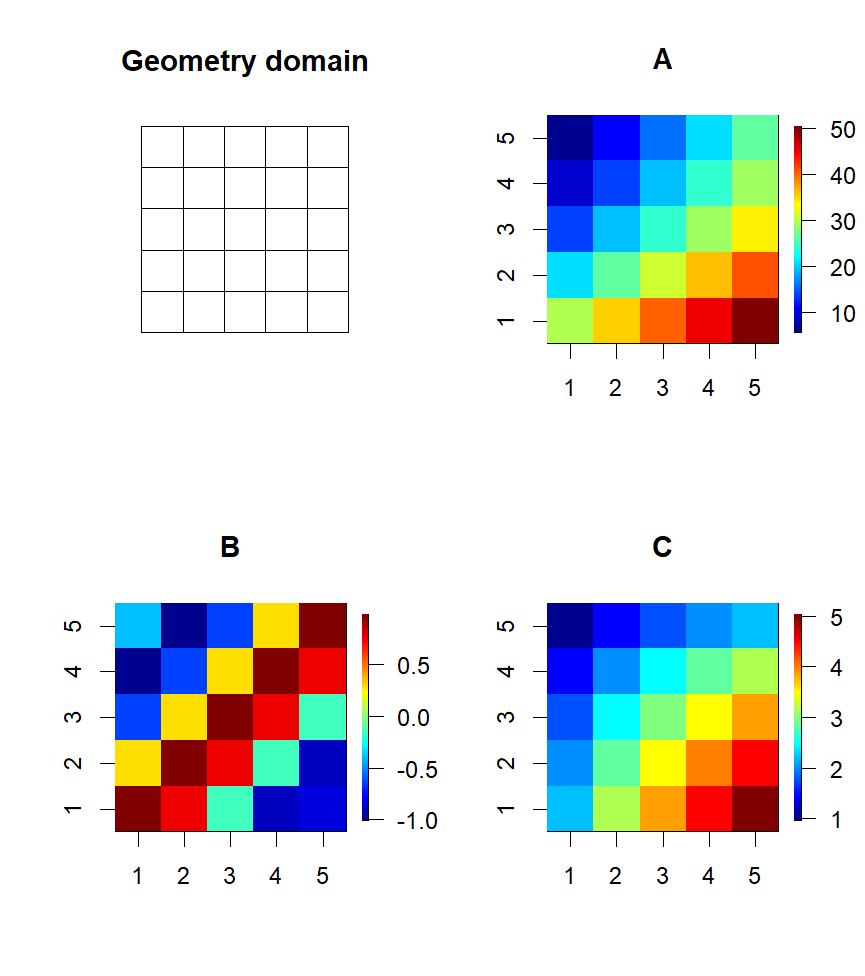
Figure 1: A demonstration of inputs for areal data with a geometry domain (top-left) and three attributes on the feature domain.

For point-level data, two data.frame object are required for the feature domain and the geometry domain. Each row of the geometry domain object is the geographical coordinate for a certain sample. We can convert these coordinates into a adjacency matrix based on a function tessellation_adjacency_matrix. The adjacency matrix relies on Voronoi tessellation of the geometry domain, such that two samples are adjacent if their Voronoi cells share a common edge. Below is an example of the conversion, and Figure 2 visualizes the result. For locations on a three-dimensional geometry domain, a Delaunay tessellation can be applied similarly. The function tessellation_adjacency_matrix will give the adjacency matrix by automatically using a suitable tessellation.

library(fields)library(alphahull)pts <- ChicagoO3$xrownames(pts) <- LETTERS[1:20]Vcells <- delvor(pts)plot(Vcells,wlines=’vor’,pch=’.’)text(pts,rownames(pts))Amat <- tessellation_adjacency_matrix(pts)

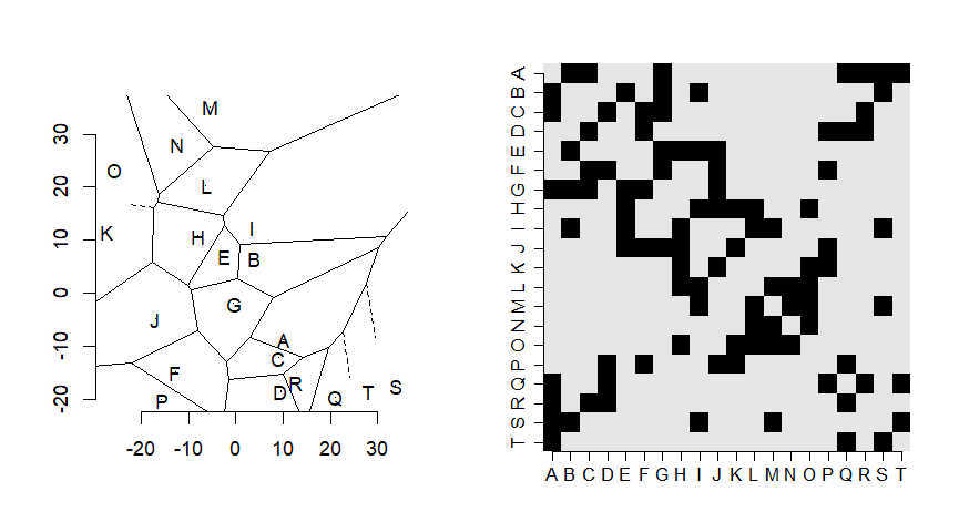
Figure 2: A demonstration of a tessellation for point-level data (left) and a heatmap of the resulting adjacent matrix, where the value of black squares is 1 (right).

Key subroutine: HCV algorithm

Before introducing the fundamental HCV clustering algorithm, we briefly describe typical agglomerative clustering without considering the information from the geometry domain. For $i=1,\ldots,n$, let $x_{i}(s_{i})=(x_{i1}(s_{i}),\ldots,x_{ip}(s_{i}))^{\prime}$ be a sample with p-dimensional attributes and $s_{i}$ is its location center on the geometry domain. The clustering algorithm starts by setting each sample as its single-element cluster, and recursively merging the pair of clusters with the smallest dissimilarity. Euclidean distance is an often used dissimilarity for pairs of samples on their $x$ values, i.e.,

$$d(x(s_{i}),x(s_{j}))=\left(\sum^{p}_{k=1}\left|x_{ik}(s_{i})-x_{jk}(s_{j})\right|^{2}\right)^{\frac{1}{2}}.$$

It is easy to see at the $t$-th iteration, there will be $n-t+1$ candidate clusters among which a pair will be merged. We denote these candidate clusters as $\{C_{h}^{t},h=1,\ldots,n-t+1\}$. A cluster may contain more than one single point, and hence, several linkage methods for determining the between-cluster dissimilarity has been proposed. The well known methods, including single, complete, average, and Ward’s methods are all follow the Lance-Williams formula with different linear coefficient (Lance and Williams, 1967) in such a form:

$$d\left(C_{h}^{\{t\}},C_{k}^{\{t+1\}}\right) =\alpha_{i}d\left(C_{i}^{\{t\}},C_{h}^{\{t\}}\right)+\alpha_{j}d\left(C_{j}^{\{t\}},C_{h}^{\{t\}}\right)+\beta d\left(C_{i}^{\{t\}},C_{j}^{\{t\}}\right)$$

$$+\gamma\left|d\left(C_{h}^{\{t\}},C_{i}^{\{t\}}\right)-d\left(C_{h}^{\{t\}},C_{j}^{\{t\}}\right)\right|,$$ (1)

where in the $(t+1)$-th iteration $C_{k}^{\{t+1\}}$ is the cluster aggregated from cluster $C_{i}^{\{t\}}$ and cluster $C_{j}^{\{t\}}$. One applies a selected linkage method recursively to compute dissimilarity, and merge the closest pair of clusters, to find a hierarchy of clusters until all samples are in a single cluster.

The idea of our HCV algorithm is generally based on the common edges of units on the geometry diagram. If any pairs of units have a common edge in the Voronoi diagram, then they are considered to have spatial proximity and geometry connectedness. In each iteration, the major difference between HCV and a typical hierarchical agglomerative clustering algorithm is that, we only focus on the geometry-connected groups. The next two candidate groups to be aggregated must share a common edge. That is, a pair of clusters $C_{h}^{\{t\}}$ and $C_{k}^{\{t\}}$ can be merged in the $(t+1)$-th iteration only if $A^{\{t\}}_{hk}=1$, where the stepwise updated adjacency matrix $A^{\{t\}}$ is recursively defined as

$$A^{\{0\}}_{ij}=\begin{cases}0,&\text{if }i=j\text{ or the }i\text{-th and }j\text{-th smaples have no common edge;}\\ 1,&\text{if the }i\text{-th and }j\text{-th samples have a common edge;}\\ \end{cases}$$ (2)

$$A_{hk}^{\{t\}}=\begin{cases}0,&\text{if }A_{hj}^{\{t-1\}}=0\text{ and }A_{hi}^{\{t-1\}}=0,\\ 1,&\text{if }A_{hj}^{\{t-1\}}=1\text{ or }A_{hi}^{\{t-1\}}=1.\\ \end{cases}$$ (3)

Putting these ideas altogether, the algorithm details of the implemented HCV function are given in Algorithm 1.

There are several linkage algorithms have been provided in HCV, including "ward", "single", "complete", "average", "weight", "median", and "centroid". Default is ’ward’. Current available methods in HCV for the dissimilarity of the feature domain are "euclidean", "correlation", "abscor", "maximum", "manhattan", "canberra", "binary" and "minkowski". Default is ’euclidean’.

Algorithm 1 Hierarchical Clustering from Vertex-links

1:Input geometry_domain, feature_domain, and linkage.

2:Set $A^{\{0\}}\equiv$ the adjacency matrix for geometry_domain using (2).

3:Calculate $D^{\{0\}}\equiv$ the dissimilarity matrix for feature_domain.

4:Set $\left\{C_{i}^{\{0\}};i=1,\ldots,n\right\}$ with each sample being a single-element cluster.

5:Set $t:=0$.

6:Create $\mathcal{T}$ as an edgeless graph for the initial tree structure.

7:Create Tree.Height as an empty array.

8:while any off-diagonal element of $A^{\{t\}}$ is nonzero  do

9:     Aggregate $C_{i}^{\{t\}}$ and $C_{j}^{\{t\}}$ into $C_{NEXT}$ if $\displaystyle\mathop{\arg\min}_{i,j,A_{ij}=1}D_{ij}^{\{t\}}$

10:     Set $t:=t+1$.

11:     Update $D^{\{t\}}$ based on (0.2.2) according to the input linkage.

12:     Update $A^{\{t\}}$ based on (3).

13:     Update Tree.Height[$t$] = $\displaystyle d\left(C_{i}^{\{t\}},C_{j}^{\{t\}}\right)$.

14:     Add $C_{NEXT}$ into $\mathcal{T}$ as a new node $C_{k}^{\{t+1\}}$.

15:     Draw edges from $C_{k}^{\{t+1\}}$ to its left and right nodes, i.e., $C_{i}^{\{t\}}$ and $C_{j}^{\{t\}}$.

16:end while

17:return Tree.Height and $\mathcal{T}$ containing list of clusters and the hierarchy

Key subroutine: Determining number of clusters

Another crucial issue in cluster analysis is to determine an appropriate number of clusters. There are several internal indices and external indices; see e.g. Desgraupes (2018). However, these indices consider only the within-cluster sum of squared difference of attributes on the feature domain, which overlooks the information on the geometry domain. In view of this, we propose a novel internal index named Spatial Mixture Index (SMI) for determining the number of clusters.

In some applications, having the number of clusters is not satisfactory enough. We may want to know the stability of clusters and their adherent members. To this end, we provide another method ‘M3C’ based on Monte Carlo simulations to find stable clusters.

Both ‘SMI’ and ‘M3C’ are available methods in the wrapper function getCluser, which provides users a more convenient tool for the number of clusters.

SMI

By connecting the pairs of points sharing common edges on the geometry domain, we have many paths between samples. Denote $\ell_{ij}$ the minimum number of paths through which $s_{i}$ can reach $s_{j}$. SMI is an internal index involving the property of spatial proximity by considering the edge length of polygons or of triangles after a tessellation. SMI is defined in (4), where ${\Delta}_{k}$ and $e_{k}$ represent the average squared distance within the $k$-th cluster for the feature domain and the geometry domain, respectively. The overall heterogeneity is a weighted sum of both squared distances for all clusters, with weights depending on $f(\cdot)$.

$$\mbox{SMI}(K)=\frac{1}{K}\sum_{k=1}^{K}\left[f(\alpha_{k}){\Delta}_{k}+(1-f(\alpha_{k}))e_{k}\right],$$ (4)

where

$${\Delta}_{k} =\frac{1}{|C_{k}|^{2}-|C_{k}|}\sum_{i\in C_{k}}\sum_{j\in C_{k}\backslash{i}}d(x_{i}(s_{i}),x_{j}(s_{j}))^{2},$$

$$e_{k} =\frac{\rho}{|C_{k}|^{2}-|C_{k}|}\sum_{i\in C_{k}}\sum_{j\in C_{k}\backslash{i}}\ell_{ij}^{2},$$

$$\rho =\frac{\sum_{i=1}^{n}\sum_{j=1}^{i-1}d(x_{i}(s_{i}),x_{j}(s_{j}))^{2}}{\sum_{i=1}^{n}\sum_{j=1}^{i-1}\ell_{ij}^{2}},$$

and $\alpha_{k}$ and the function $f$ are defined as follows:

$$\alpha_{k} =\frac{Ke_{k}-\sum_{j=1}^{K}e_{j}}{\sum_{j=1}^{K}e_{j}},$$

$$f(x) =(1+e^{-x})^{-1}.$$

The squared distances are analogous to within-cluster sum of squares, and $\rho$ deals with potiential different scales between ${\Delta}_{k}$ and $e_{k}$. We suggest to use $K^{*}=\mbox{arg min}_{K}\mbox{SMI}(K)/\mbox{SMI}(K-1)$ for selecting the number of clusters. Our getCluster fucntion has a method argument. If method = ‘SMI’ is specified, values of SMI from 2 to Kmax clusters will be compared, and individual cluster members are reported, under the selected number of clusters based on SMI.

M3C

We modified a method in the M3C package (John et al., 2018) to take the uncertainty of cluster into account via Monte Carlo simulations and calculating the consensus matrix. M3C compares the result of the clusters at hand with the clusters generated by simulations, and it determines the appropriate number of clusters based on the most significant proportion of ambiguous clustering (PAC) score. As its design is not for spatial data clustering, M3C does not consider the information on the geometry domain. We construct a geometry embedded dissimilarity matrix (GEDM) to fill the gap, and the procedure is explained in the following.

Our method utilizes the output of the HCV algorithm, which carries information of the dissimilarity between clusters and the constraints on the geometry. We turn such information into a GEDM through Algorithm 2. Then the GEDM is converted into Euclidean coordinates using a metric multidimensional scaling, followed by applying Monte Carlo reference-based consensus clustering of the M3C package. The default score to evaluate cluster stability is PAC score, but users can specify an alternative score in the criterion argument when necessary.

Similar to that with method = ‘SMI’, if method = ‘M3C’ is used in the implemented getCluster fucntion, individual cluster members are reported, under the selected number of clusters having the smallest score.

Algorithm 2 Geometry Embedded Dissimilarity Matrix

1:Input an HCV object with Tree.Height and $\mathcal{T}$.

2:Set I_max the length of Tree.Height in the input HCV object

3:Create a matrix $M$ with zero diagonals and all off-diagonals being Tree.Height[I_max].

4:Set GEDM $:=M$.

5:for $t$ from I_max to 1 do

6:     LeftMembers := members in LeftNode of $C_{k}^{\{t\}}$ in $\mathcal{T}$

7:     RightMembers := members in RightNode of $C_{k}^{\{t\}}$ in $\mathcal{T}$

8:     for $\ell$ in LeftMembers do

9:         for $r$ in RightMembers do

10:              GEDM[$\ell$, $r$] = $\min$(Tree.Height[$t$], GEDM[$\ell$,$r$])

11:              GEDM[$r$, $\ell$] = GEDM[$\ell$, $r$]

12:         end for

13:     end for

14:end for

15:return GEDM

Simulation Examples and Real Data

Simulation data

We used the way to generate synthetic point-level data propose by Lin et al. (2005) as follows. The procedure is also implemented as the synthetic_data function in our package.

1. Specify the number of clusters $(k)$, number of points $(n)$, the dimension of feature domain $(p_{1})$ and geometry domain $(p_{2})$.

2. Select exactly $k$ points from the domain $(0,1)^{p_{1}}$ randomly as the center of the $k$ clusters on feature domain, i.e., $\mu^{feat}_{1},\ldots,\mu^{feat}_{k}$.

3. Select exactly $k$ points from the domain $(0,1)^{p_{2}}$ randomly as the center of the $k$ clusters on geometry domain, i.e., $\mu^{geo}_{1},\ldots,\mu^{geo}_{k}$

4. Draw a random point $o$ from joint uniform distribution over the geometry domain.

5. Assign point $o$ to $C_{i}$ by the probability mass function (PMF) as $P(o\in C_{i})=\frac{d\left(o,\mu^{geo}_{i}\right)^{-f}}{\sum_{j=1}^{k}{d\left(o,\mu^{geo}_{j}\right)^{-f}}}$

6. Draw a sample form joint normal distribution $N(\mu_{i}^{feat},r^{2}I)$ as the feature domain attribute for the point $o$ in Step 4.

7. Repeat Step 4 to 6 until $n$ points have been sampled.

In the above process, $C_{i}^{feat},C_{i}^{geo}$ are the centers of feature domain and geometry domain of the cluster $C_{i}$ respectively. It is easy to see that the parameter $f$ controls the degree of spatial homogeneity in step 5. the larger $f$ value presents, the more spatial homogeneity has been introduced, and we controls the variation of the feature domain attribute by parameter $r$.

Here we present an example for clustering of point-level data. The parameters of synthetic data were $(k,f,r,n,p_{1},p_{2})=(3,30,0.02,300,2,2)$.

set.seed(0)pcase <- synthetic_data(3,30,0.02,300,2,2)labcolor <- (pcase$labels+1)%%3+1par(mfrow = c(1,2))plot(pcase$feat, col = labcolor, pch=19, xlab = ’First attribute’,     ylab = ’Second attribute’, main = ’Feature domain’)plot(pcase$geo, col = labcolor, pch=19, xlab = ’First attribute’,     ylab = ’Second attribute’, main = ’Geometry domain’)

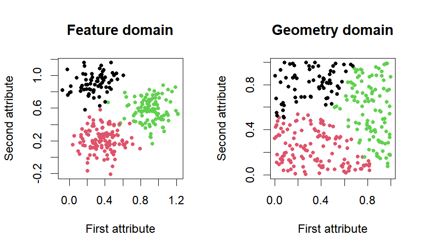
Figure 3: The feature domain and the geometry domain of the simulated point-level data, where distinct colors stand for different clusters.

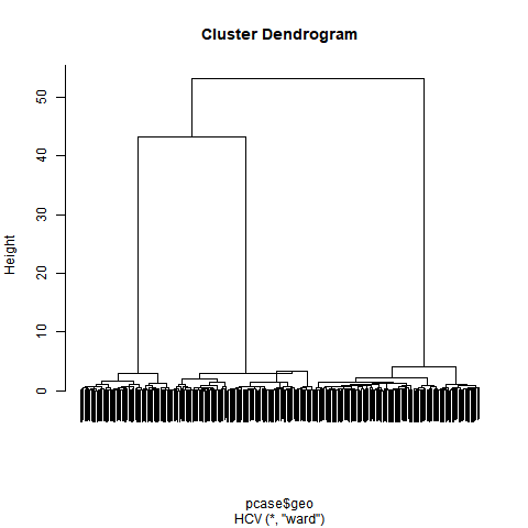
Figure 4: The cluster dendrogram for the simulated data on Figure 3 using HCV.

The simulated data are shown in Figure 3. We then compare the results from our package using method=’SMI’ with that from the SPODT package. The detailed codes are given below. Since HCV outputs an hclust object, we can easily plot the dengrogram as Figure 4shown, and use cutree to form final clusters. However, a closer examination will reveal that crossovers or inversions occur on such a dendrogram, and hence cutree should be applied with care. We recommend getCluster instead for determining clusters. The found clusters are shown in Figure 5. As can be seen, the proposed method almost recovers the true clusters, while there are more mismatches based on SPODT.

# clustering with HCVHCVobj <- HCV(pcase$geo, pcase$feat)smi <- getCluster(HCVobj,method="SMI")plot(HCVobj)# clustering with SPODTlibrary(cluster)library(SPODT)grp <- pam(pcase$feat,k=3)dataset <- data.frame(pcase$geo,grp$clustering)colnames(dataset) <- c(’x1’,’x2’,’grp’)coordinates(dataset) <- c("x1","x2")spc <- spodt(dataset@data$grp~1, dataset, graft = 0.3)# plots for resultspar(mfrow=c(2,2))plot(pcase$feat, col=factor(smi),pch=19, xlab = ’First attribute’,     ylab = ’Second attribute’,main = ’Feature domain’)plot(pcase$geo, col=factor(smi),pch=19, xlab = ’First attribute’,     ylab = ’Second attribute’,main = ’Geometry domain’)plot(pcase$feat, col=factor(spc@partition),pch=19, xlab = ’First attribute’,     ylab = ’Second attribute’,main = ’Feature domain’)plot(pcase$geo, col=factor(spc@partition),pch=19, xlab = ’First attribute’,     ylab = ’Second attribute’,main = ’Geometry domain’)

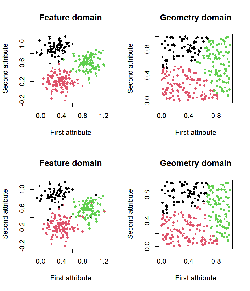
Figure 5: The scatterplot with found clusters using the HCV algorithm (top panel) and using the SPODT package (bottom panel), where distinct colors stand for different clusters in each method.

Real application: French municipalities data

We used the estuary data in the ClustGeo package, which involved 303 France cities located along Gironde estuary. There are four attributes on the feaure domain: city employee rate, city graduation rate, ratio of apartment housing and agricultural area, and these are areal data on the geometry domain. For understanding the spatial distribution of the four features, we visualize via heatmaps and represent the magnitude of standardized features in Figure 6. It is obvious that there are several potential outliers in city employee rate and ratio of apartment housing that have extremely large values.

library(ClustGeo)library(fields)data(estuary)colors <- tim.colors(303)lim <- c(-2.5,2.5)dat <- estuary$datplotMap(estuary$map, scale(dat[,1]), color=colors, zlim=lim, bar=’employ’)plotMap(estuary$map, scale(dat[,2]), color=colors, zlim=lim, bar=’grad’)plotMap(estuary$map, scale(dat[,3]), color=colors, zlim=lim, bar=’housing’)plotMap(estuary$map, scale(dat[,4]), color=colors, zlim=lim, bar=’agriland’)

In this example, we present to input a user-specified dissimilarity matrix and adjacency matrix, by setting diss = ’precomputed’ and adjacency = TRUE as the codes given below. We use squared Euclidean distance as the dissimilarity, and covert the SpatialPolygonsDataFrame object estuary$map to an adjacency matrix. After calling the HCV function, we apply the getCluster function with method=’M3C’ to find the most stable clusters. We also compare it with the clusters found by ClustGeo. The result are shown in Figure 7. Some cluster patterns are quite similar in the two methods, although ClustGeo has more spatially fragmented clusters. If spatial contiguity is of interest, the HCV algorithm is preferred.

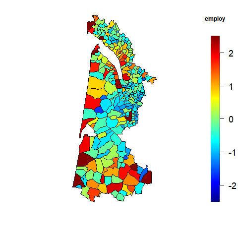
(a) City employee rate

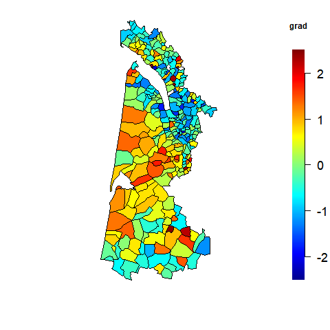
(b) City graduation rate

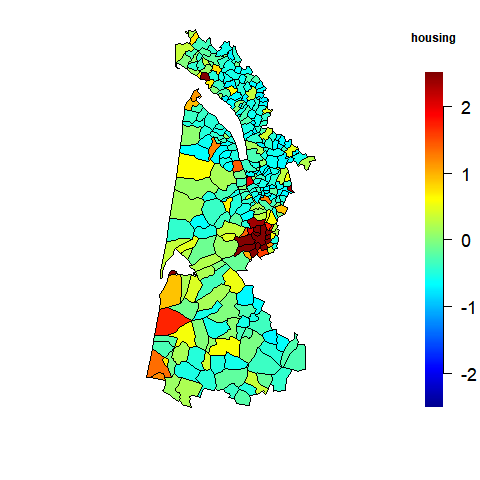
(c) Ratio of apartment housing

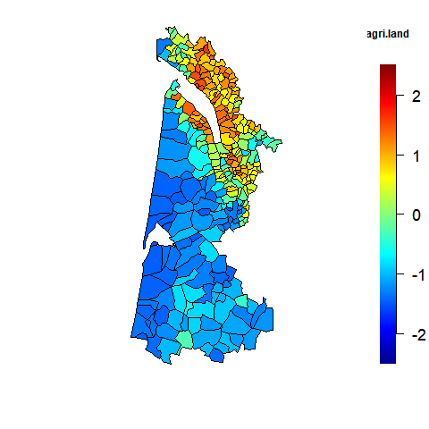
(d) Agricultural area

Figure 6: Heatmaps for standardized values of the four socio-economic variables in the estuary data.

# clustering with HCVfeat <- as.matrix(scale(dat))fdist <- as.matrix(dist(feat)) ** 2geo <- estuary$mapadj <- rgeos::gTouches(geo, byid=TRUE) * 1tree1 <- HCV(adj, fdist,  adjacency = T, diss = ’precomputed’)m3c <- getCluster(tree1, method=’M3C’)# clustering with ClustGeoD0 <- dist(scale(dat))D1 <- as.dist(1-adj)tree2 <- hclustgeo(D0,D1,alpha=0.4)cg <- cutree(tree2,7)# plots for resultspar(mfrow=c(1,2),mar=c(0,0,0,0))plot(geo, col = tim.colors(7)[m3c], border=’grey’)plot(map,border="grey",col=tim.colors(7)[cg])

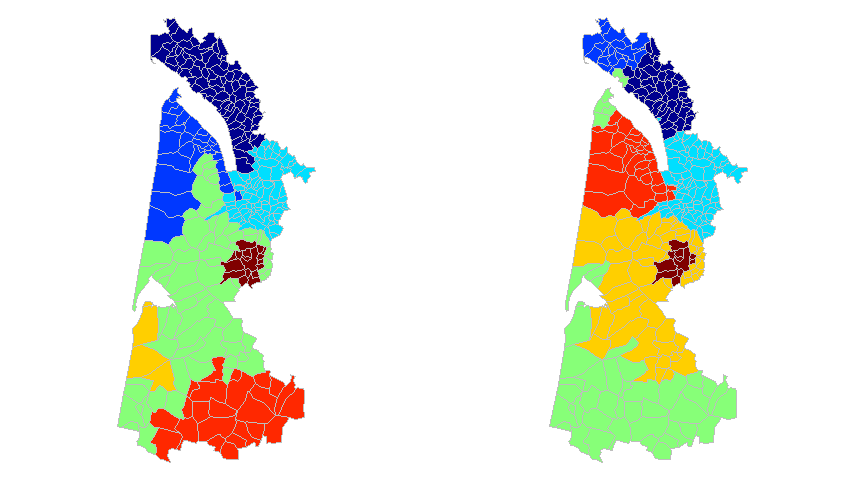
Figure 7: The found clusters using the HCV algorithm (left) and using the ClustGeo package (right), where distinct colors stand for different clusters in each method.

Summary

In this paper, the R package HCV is presented for spatial data clustering with the contiguity property. We modified hierarchical agglomerative clustering algorithms and methods for determining the number of clusters, such that the spatial information on the geometry domain can be reasonablly incorproated. We demonstrate the package applications to point-level data and areal data. By these examples, we show that HCV is a unified framework for clustering both types of spatial data.

ShengLi Tzeng
Department of Applied Mathematics
National Sun Yat-sen University
Kaohsiung, Taiwan, 80424
slt.cmu@gmail.com

Hao-Yun Hsu
Department of Applied Mathematics
National Sun Yat-sen University
Kaohsiung, Taiwan, 80424
zoez5230100@gmail.com

References

- Assunção et al. (2006) R. M. Assunção, M. C. Neves, G. Câmara, and C. da Costa Freitas. Efficient regionalization techniques for socio-economic geographical units using minimum spanning trees. International Journal of Geographical Information Science, 20(7):797–811, 2006.
- Banerjee et al. (2003) S. Banerjee, B. P. Carlin, and A. E. Gelfand. Hierarchical modeling and analysis for spatial data. Chapman and Hall/CRC, 2003.
- Carvalho et al. (2009) A. X. Y. Carvalho, P. H. M. Albuquerque, G. R. de Almeida Junior, and R. D. Guimaraes. Spatial hierarchical clustering. Revista Brasileira de Biometria, 27(3):411–442, 2009.
- Chavent et al. (2018) M. Chavent, V. Kuentz-Simonet, A. Labenne, and J. Saracco. Clustgeo: an r package for hierarchical clustering with spatial constraints. Computational Statistics, 33(4):1799–1822, 2018.
- Chew (1989) L. P. Chew. Constrained delaunay triangulations. Algorithmica, 4(1):97–108, 1989.
- Cressie (1993) N. Cressie. Statistics for spatial data. John Wiley & Sons, Hoboken, NJ, revised edition, 1993.
- Desgraupes (2018) B. Desgraupes. clusterCrit: Clustering Indices, 2018. URL https://CRAN.R-project.org/package=clusterCrit. R package version 1.2.8.
- Gaudart et al. (2015) J. Gaudart, N. Graffeo, D. Coulibaly, G. Barbet, S. Rebaudet, N. Dessay, O. K. Doumbo, and R. Giorgi. SPODT: An R package to perform spatial partitioning. Journal of Statistical Software, 63(16):1–23, 2015. URL http://www.jstatsoft.org/v63/i16/.
- John et al. (2018) C. R. John, D. Watson, M. Lewis, D. Russ, K. Goldmann, M. Ehrenstein, C. Pitzalis, and M. Barnes. M3c: A monte carlo reference-based consensus clustering algorithm. bioRxiv, 2018. doi: https://doi.org/10.1101/377002.
- Kriegel et al. (2011) H.-P. Kriegel, P. Kröger, J. Sander, and A. Zimek. Density-based clustering. Wiley Interdisciplinary Reviews: Data Mining and Knowledge Discovery, 1(3):231–240, 2011.
- Lance and Williams (1967) G. N. Lance and W. T. Williams. A general theory of classificatory sorting strategies: 1. hierarchical systems. The computer journal, 9(4):373–380, 1967.
- Liao and Peng (2012) Z.-X. Liao and W.-C. Peng. Clustering spatial data with a geographic constraint: exploring local search. Knowledge and information systems, 31(1):153–170, 2012.
- Lin et al. (2005) C.-R. Lin, K.-H. Liu, and M.-S. Chen. Dual clustering: integrating data clustering over optimization and constraint domains. IEEE Transactions on Knowledge and Data Engineering, 17(5):628–637, 2005.
- Xie (2019) S. Xie. Defining geographical rating territories in auto insurance regulation by spatially constrained clustering. Risks, 7(2):42, 2019.
- Zhou et al. (2007) J. Zhou, J. Guan, and P. Li. Dcad: a dual clustering algorithm for distributed spatial databases. Geo-spatial Information Science, 10(2):137–144, 2007.