2 Stochastic Hamiltonian PDEs
Stochastic Hamiltonian PDEs, as natural extensions of stochastic
Hamiltonian ordinary differential equations, play important roles in the fields of fluid dynamics, nonlinear optics, plasma physics, communications and medical science and so forth.
They are due to [11 ] and given by
M d z + K z x d t = ∇ S 1 ( z ) d t + ∇ S 2 ( z ) ∘ d W ( t ) , 𝑀 𝑑 𝑧 𝐾 subscript 𝑧 𝑥 𝑑 𝑡 ∇ subscript 𝑆 1 𝑧 𝑑 𝑡 ∇ subscript 𝑆 2 𝑧 𝑑 𝑊 𝑡 Mdz+Kz_{x}dt=\nabla S_{1}(z)dt+\nabla S_{2}(z)\circ dW(t), (2.1)
where x ∈ 𝒪 , 𝑥 𝒪 x\in\mathcal{O}, M 𝑀 M K 𝐾 K S 1 subscript 𝑆 1 S_{1} S 2 subscript 𝑆 2 S_{2} z 𝑧 z ∘ \circ { W ( t ) } t ≥ 0 subscript 𝑊 𝑡 𝑡 0 \{W(t)\}_{t\geq 0} 𝕃 2 ( 𝒪 , ℝ ) superscript 𝕃 2 𝒪 ℝ \mathbb{L}^{2}(\mathcal{O},\mathbb{R}) Q 𝑄 Q { ℱ t } t ≥ 0 subscript subscript ℱ 𝑡 𝑡 0 \{\mathcal{F}_{t}\}_{t\geq 0} ( Ω , ℱ , { ℱ t } t ≥ 0 , ℙ ) Ω ℱ subscript subscript ℱ 𝑡 𝑡 0 ℙ (\Omega,\mathcal{F},\{\mathcal{F}_{t}\}_{t\geq 0},\mathbb{P})
W ( t ) = ∑ k = 1 ∞ q k e k β k ( t ) , 𝑊 𝑡 superscript subscript 𝑘 1 subscript 𝑞 𝑘 subscript 𝑒 𝑘 subscript 𝛽 𝑘 𝑡 W(t)=\sum_{k=1}^{\infty}\sqrt{q_{k}}e_{k}\beta_{k}(t),
where { ( q k , e k ) } k = 1 ∞ superscript subscript subscript 𝑞 𝑘 subscript 𝑒 𝑘 𝑘 1 \{(q_{k},e_{k})\}_{k=1}^{\infty} Q 𝑄 Q { β k ( t ) } k = 1 ∞ superscript subscript subscript 𝛽 𝑘 𝑡 𝑘 1 \{\beta_{k}(t)\}_{k=1}^{\infty} 2.1
1.
by introducing v = u t 𝑣 subscript 𝑢 𝑡 v=u_{t} w = u x 𝑤 subscript 𝑢 𝑥 w=u_{x}
d u t − u x x d t + f ( u ) d t = g ( u ) ∘ d W ( t ) 𝑑 subscript 𝑢 𝑡 subscript 𝑢 𝑥 𝑥 𝑑 𝑡 𝑓 𝑢 𝑑 𝑡 𝑔 𝑢 𝑑 𝑊 𝑡 du_{t}-u_{xx}dt+f(u)dt=g(u)\circ dW(t)
into
{ d u = v d t , u x = w , d v − w x d t = − f ( u ) d t + g ( u ) ∘ d W ( t ) , \left\{\begin{aligned} &du=vdt,\\
&u_{x}=w,\\
&dv-w_{x}dt=-f(u)dt+g(u)\circ dW(t),\end{aligned}\right. (2.2)
where f : 𝕃 2 ( 𝒪 , ℝ ) → 𝕃 2 ( 𝒪 , ℝ ) : 𝑓 → superscript 𝕃 2 𝒪 ℝ superscript 𝕃 2 𝒪 ℝ f:\mathbb{L}^{2}(\mathcal{O},\mathbb{R})\rightarrow\mathbb{L}^{2}(\mathcal{O},\mathbb{R}) g : 𝕃 2 ( 𝒪 , ℝ ) → ℒ 2 ( 𝕃 2 ( 𝒪 , ℝ ) , Q 1 2 ( 𝕃 2 ( 𝒪 , ℝ ) ) ) : 𝑔 → superscript 𝕃 2 𝒪 ℝ subscript ℒ 2 superscript 𝕃 2 𝒪 ℝ superscript 𝑄 1 2 superscript 𝕃 2 𝒪 ℝ g:\mathbb{L}^{2}(\mathcal{O},\mathbb{R})\rightarrow\mathscr{L}_{2}(\mathbb{L}^{2}(\mathcal{O},\mathbb{R}),Q^{\frac{1}{2}}(\mathbb{L}^{2}(\mathcal{O},\mathbb{R}))) 𝒪 = [ x L , x R ] , 𝒪 subscript 𝑥 𝐿 subscript 𝑥 𝑅 \mathcal{O}=\left[x_{L},x_{R}\right], x L , x R ∈ ℝ , subscript 𝑥 𝐿 subscript 𝑥 𝑅
ℝ x_{L},x_{R}\in\mathbb{R}, ℒ 2 ( 𝕃 2 ( 𝒪 , ℝ ) , Q 1 2 ( 𝕃 2 ( 𝒪 , ℝ ) ) ) subscript ℒ 2 superscript 𝕃 2 𝒪 ℝ superscript 𝑄 1 2 superscript 𝕃 2 𝒪 ℝ \mathscr{L}_{2}(\mathbb{L}^{2}(\mathcal{O},\mathbb{R}),Q^{\frac{1}{2}}(\mathbb{L}^{2}(\mathcal{O},\mathbb{R}))) z = ( u , p , v , w ) ⊤ , 𝑧 superscript 𝑢 𝑝 𝑣 𝑤 top z=(u,p,v,w)^{\top}, 2.2
M d z + K z x d t = ∇ S 1 ( z ) d t + ∇ S 2 ( z ) ∘ d W ( t ) 𝑀 𝑑 𝑧 𝐾 subscript 𝑧 𝑥 𝑑 𝑡 ∇ subscript 𝑆 1 𝑧 𝑑 𝑡 ∇ subscript 𝑆 2 𝑧 𝑑 𝑊 𝑡 Mdz+Kz_{x}dt=\nabla S_{1}(z)dt+\nabla S_{2}(z)\circ dW(t)
with
M = ( 0 0 1 0 0 0 0 0 − 1 0 0 0 0 0 0 0 ) , K = ( 0 0 0 − 1 0 0 0 0 0 0 0 0 1 0 0 0 ) , formulae-sequence 𝑀 0 0 1 0 0 0 0 0 1 0 0 0 0 0 0 0 𝐾 0 0 0 1 0 0 0 0 0 0 0 0 1 0 0 0 \displaystyle M=\left(\begin{array}[]{cccc}0&0&1&0\\
0&0&0&0\\
-1&0&0&0\\
0&0&0&0\\
\end{array}\right),\quad K=\left(\begin{array}[]{cccc}0&0&0&-1\\
0&0&0&0\\
0&0&0&0\\
1&0&0&0\\
\end{array}\right),
S 1 ( z ) = 1 2 ( w 2 − v 2 ) − f ~ ( u ) , S 2 ( z ) = g ~ ( u ) , formulae-sequence subscript 𝑆 1 𝑧 1 2 superscript 𝑤 2 superscript 𝑣 2 ~ 𝑓 𝑢 subscript 𝑆 2 𝑧 ~ 𝑔 𝑢 \displaystyle S_{1}(z)=\frac{1}{2}\left(w^{2}-v^{2}\right)-\tilde{f}(u),\quad S_{2}(z)=\tilde{g}(u),
where f = f ~ u 𝑓 subscript ~ 𝑓 𝑢 f=\tilde{f}_{u} g = g ~ u 𝑔 subscript ~ 𝑔 𝑢 g=\tilde{g}_{u} [18 ] ).
2.
consider the stochastic nonlinear Schrödinger equation under the homogenous Dirichlet boundary condition
𝐢 d u + u x x d t + | u | 2 u d t = u ∘ d W ( t ) 𝐢 𝑑 𝑢 subscript 𝑢 𝑥 𝑥 𝑑 𝑡 superscript 𝑢 2 𝑢 𝑑 𝑡 𝑢 𝑑 𝑊 𝑡 \mathbf{i}du+u_{xx}dt+|u|^{2}udt=u\circ dW(t)
with 𝒪 = [ 0 , 1 ] 𝒪 0 1 \mathcal{O}=[0,1] 𝐢 2 = − 1 superscript 𝐢 2 1 \mathbf{i}^{2}=-1 u = p + 𝐢 q 𝑢 𝑝 𝐢 𝑞 u=p+\mathbf{i}q v = p x 𝑣 subscript 𝑝 𝑥 v=p_{x} w = q x 𝑤 subscript 𝑞 𝑥 w=q_{x}
{ d q − v x d t = ( p 2 + q 2 ) p d t − p ∘ d W ( t ) , d p + w x d t = − ( p 2 + q 2 ) q d t + q ∘ d W ( t ) , p x = v , q x = w . \left\{\begin{aligned} &dq-v_{x}dt=\left(p^{2}+q^{2}\right)pdt-p\circ dW(t),\\
&dp+w_{x}dt=-\left(p^{2}+q^{2}\right)qdt+q\circ dW(t),\\
&p_{x}=v,\\
&q_{x}=w.\end{aligned}\right. (2.3)
Defining a state variable z = ( p , q , v , w ) ⊤ 𝑧 superscript 𝑝 𝑞 𝑣 𝑤 top z=(p,q,v,w)^{\top} [11 ] presents the associated multi-symplectic form of (2.3
M d z + K z x d t = ∇ S 1 ( z ) d t + ∇ S 2 ( z ) ∘ d W ( t ) 𝑀 𝑑 𝑧 𝐾 subscript 𝑧 𝑥 𝑑 𝑡 ∇ subscript 𝑆 1 𝑧 𝑑 𝑡 ∇ subscript 𝑆 2 𝑧 𝑑 𝑊 𝑡 Mdz+Kz_{x}dt=\nabla S_{1}(z)dt+\nabla S_{2}(z)\circ dW(t)
with
M = ( 0 − 1 0 0 1 0 0 0 0 0 0 0 0 0 0 0 ) , K = ( 0 0 1 0 0 0 0 1 − 1 0 0 0 0 − 1 0 0 ) , formulae-sequence 𝑀 0 1 0 0 1 0 0 0 0 0 0 0 0 0 0 0 𝐾 0 0 1 0 0 0 0 1 1 0 0 0 0 1 0 0 \displaystyle M=\left(\begin{array}[]{cccc}0&-1&0&0\\
1&0&0&0\\
0&0&0&0\\
0&0&0&0\\
\end{array}\right),\quad K=\left(\begin{array}[]{cccc}0&0&1&0\\
0&0&0&1\\
-1&0&0&0\\
0&-1&0&0\\
\end{array}\right),
S 1 ( z ) = − 1 4 ( p 2 + q 2 ) 2 − 1 2 ( v 2 + w 2 ) , S 2 ( z ) = 1 2 ( p 2 + q 2 ) . formulae-sequence subscript 𝑆 1 𝑧 1 4 superscript superscript 𝑝 2 superscript 𝑞 2 2 1 2 superscript 𝑣 2 superscript 𝑤 2 subscript 𝑆 2 𝑧 1 2 superscript 𝑝 2 superscript 𝑞 2 \displaystyle S_{1}(z)=-\frac{1}{4}\left(p^{2}+q^{2}\right)^{2}-\frac{1}{2}\left(v^{2}+w^{2}\right),\quad S_{2}(z)=\frac{1}{2}\left(p^{2}+q^{2}\right).
3.
the stochastic Korteweg-de Vries equation with the homogenous Dirichlet boundary condition takes the form
d u + u u x d t + β u x x x d t = λ d W ( t ) , 𝑑 𝑢 𝑢 subscript 𝑢 𝑥 𝑑 𝑡 𝛽 subscript 𝑢 𝑥 𝑥 𝑥 𝑑 𝑡 𝜆 𝑑 𝑊 𝑡 du+uu_{x}dt+\beta u_{xxx}dt=\lambda dW(t),
where β , λ > 0 𝛽 𝜆
0 \beta,\lambda>0 𝒪 = [ 0 , 1 ] 𝒪 0 1 \mathcal{O}=[0,1] v , ρ , w 𝑣 𝜌 𝑤
v,\rho,w
{ − 1 2 d ρ − β w x d t = 1 2 u 2 d t − v d t , ρ x = u , 1 2 d u + v x d t = λ d W ( t ) , u x = w , \left\{\begin{aligned} &-\frac{1}{2}d\rho-\beta w_{x}dt=\frac{1}{2}u^{2}dt-vdt,\\
&\rho_{x}=u,\\
&\frac{1}{2}du+v_{x}dt=\lambda dW(t),\\
&u_{x}=w,\end{aligned}\right. (2.4)
we have the compact form (see [1 ] )
M d z + K z x d t = ∇ S 1 ( z ) d t + ∇ S 2 ( z ) ∘ d W ( t ) 𝑀 𝑑 𝑧 𝐾 subscript 𝑧 𝑥 𝑑 𝑡 ∇ subscript 𝑆 1 𝑧 𝑑 𝑡 ∇ subscript 𝑆 2 𝑧 𝑑 𝑊 𝑡 Mdz+Kz_{x}dt=\nabla S_{1}(z)dt+\nabla S_{2}(z)\circ dW(t)
with z = ( u , v , ρ , w ) ⊤ , 𝑧 superscript 𝑢 𝑣 𝜌 𝑤 top z=(u,v,\rho,w)^{\top},
M = ( 0 0 − 1 2 0 0 0 0 0 1 2 0 0 0 0 0 0 0 ) , K = ( 0 0 0 − β 0 0 − 1 0 0 1 0 0 β 0 0 0 ) , S 1 ( z ) = 1 6 u 3 − u v + 1 2 β w 2 , S 2 ( z ) = λ ρ . formulae-sequence 𝑀 0 0 1 2 0 0 0 0 0 1 2 0 0 0 0 0 0 0 formulae-sequence 𝐾 0 0 0 𝛽 0 0 1 0 0 1 0 0 𝛽 0 0 0 formulae-sequence subscript 𝑆 1 𝑧 1 6 superscript 𝑢 3 𝑢 𝑣 1 2 𝛽 superscript 𝑤 2 subscript 𝑆 2 𝑧 𝜆 𝜌 \displaystyle M=\left(\begin{array}[]{cccc}0&0&-\frac{1}{2}&0\\
0&0&0&0\\
\frac{1}{2}&0&0&0\\
0&0&0&0\\
\end{array}\right),~{}K=\left(\begin{array}[]{cccc}0&0&0&-\beta\\
0&0&-1&0\\
0&1&0&0\\
\beta&0&0&0\\
\end{array}\right),~{}S_{1}(z)=\frac{1}{6}u^{3}-uv+\frac{1}{2}\beta w^{2},\quad S_{2}(z)=\lambda\rho.
4.
take the stochastic Maxwell equation with multiplicative noise
{ d 𝐄 ( t , x , y , z ) = ∇ × 𝐇 ( t , x , y , z ) − λ 𝐇 ( t , x , y , z ) ∘ d W ( t ) , d 𝐇 ( t , x , y , z ) = − ∇ × 𝐄 ( t , x , y , z ) + λ 𝐄 ( t , x , y , z ) ∘ d W ( t ) \left\{\begin{aligned} &d\mathbf{E}(t,x,y,z)=\nabla\times\mathbf{H}(t,x,y,z)-\lambda\mathbf{H}(t,x,y,z)\circ dW(t),\\
&d\mathbf{H}(t,x,y,z)=-\nabla\times\mathbf{E}(t,x,y,z)+\lambda\mathbf{E}(t,x,y,z)\circ dW(t)\end{aligned}\right. (2.5)
into account,
where λ ∈ ℝ , 𝜆 ℝ \lambda\in\mathbb{R}, 𝒪 ⊂ ℝ 3 𝒪 superscript ℝ 3 \mathcal{O}\subset\mathbb{R}^{3} ∂ 𝒪 𝒪 \partial\mathcal{O} 𝐄 × 𝐧 = 𝟎 𝐄 𝐧 0 \mathbf{E}\times\mathbf{n}=\mathbf{0} ( 0 , T ] × ∂ 𝒪 0 𝑇 𝒪 (0,T]\times\partial\mathcal{O} 𝐧 𝐧 \mathbf{n} ∂ 𝒪 𝒪 \partial\mathcal{O} [8 ] ).
Denote 𝐮 = ( 𝐇 ⊤ , 𝐄 ⊤ ) ⊤ = ( H 1 , H 2 , H 3 , E 1 , E 2 , E 3 ) ⊤ 𝐮 superscript superscript 𝐇 top superscript 𝐄 top top superscript subscript 𝐻 1 subscript 𝐻 2 subscript 𝐻 3 subscript 𝐸 1 subscript 𝐸 2 subscript 𝐸 3 top \mathbf{u}=(\mathbf{H}^{\top},\mathbf{E}^{\top})^{\top}=\left(H_{1},H_{2},H_{3},E_{1},E_{2},E_{3}\right)^{\top} S ( 𝐮 ) = λ 2 ( | E 1 | 2 + | E 2 | 2 + | E 3 | 2 + | H 1 | 2 + | H 2 | 2 + | H 3 | 2 ) . 𝑆 𝐮 𝜆 2 superscript subscript 𝐸 1 2 superscript subscript 𝐸 2 2 superscript subscript 𝐸 3 2 superscript subscript 𝐻 1 2 superscript subscript 𝐻 2 2 superscript subscript 𝐻 3 2 S({\bf u})=\frac{\lambda}{2}\left(\left|E_{1}\right|^{2}+\left|E_{2}\right|^{2}+\left|E_{3}\right|^{2}+\left|H_{1}\right|^{2}+\left|H_{2}\right|^{2}+\left|H_{3}\right|^{2}\right). 2.5
M d 𝐮 + K 1 𝐮 x d t + K 2 𝐮 y d t + K 3 𝐮 z d t = ∇ S ( 𝐮 ) ∘ d W , 𝑀 𝑑 𝐮 subscript 𝐾 1 subscript 𝐮 𝑥 𝑑 𝑡 subscript 𝐾 2 subscript 𝐮 𝑦 𝑑 𝑡 subscript 𝐾 3 subscript 𝐮 𝑧 𝑑 𝑡 ∇ 𝑆 𝐮 𝑑 𝑊 Md\mathbf{u}+K_{1}\mathbf{u}_{x}dt+K_{2}\mathbf{u}_{y}dt+K_{3}\mathbf{u}_{z}dt=\nabla S({\bf u})\circ dW, (2.6)
where
M = ( 0 − I 3 × 3 I 3 × 3 0 ) , K i = ( 𝒟 i 0 0 𝒟 i ) , i = 1 , 2 , 3 formulae-sequence 𝑀 0 subscript 𝐼 3 3 subscript 𝐼 3 3 0 formulae-sequence subscript 𝐾 𝑖 subscript 𝒟 𝑖 0 0 subscript 𝒟 𝑖 𝑖 1 2 3
M=\left(\begin{array}[]{cc}0&-I_{3\times 3}\\
I_{3\times 3}&0\end{array}\right),\quad K_{i}=\left(\begin{array}[]{cc}\mathscr{D}_{i}&0\\
0&\mathscr{D}_{i}\end{array}\right),\quad i=1,2,3
with I 3 × 3 subscript 𝐼 3 3 I_{3\times 3} 3 × 3 3 3 3\times 3
𝒟 1 = ( 0 0 0 0 0 − 1 0 1 0 ) , 𝒟 2 = ( 0 0 1 0 0 0 − 1 0 0 ) , 𝒟 3 = ( 0 − 1 0 1 0 0 0 0 0 ) . formulae-sequence subscript 𝒟 1 0 0 0 0 0 1 0 1 0 formulae-sequence subscript 𝒟 2 0 0 1 0 0 0 1 0 0 subscript 𝒟 3 0 1 0 1 0 0 0 0 0 \mathscr{D}_{1}=\left(\begin{array}[]{ccc}0&0&0\\
0&0&-1\\
0&1&0\end{array}\right),\quad\mathscr{D}_{2}=\left(\begin{array}[]{ccc}0&0&1\\
0&0&0\\
-1&0&0\end{array}\right),\quad\mathscr{D}_{3}=\left(\begin{array}[]{ccc}0&-1&0\\
1&0&0\\
0&0&0\end{array}\right).
Analogues to the symplecticity-preserving property of stochastic Hamiltonian ordinary differential equations, [11 ] shows that stochastic Hamiltonian PDEs possess the multi-symplectic conservation law.
In detail, denote two differential 2-forms by ω = d z ∧ M d z 𝜔 d 𝑧 𝑀 d 𝑧 \omega=\mathrm{d}z\wedge M\mathrm{d}z κ = d z ∧ K d z , 𝜅 d 𝑧 𝐾 d 𝑧 \kappa=\mathrm{d}z\wedge K\mathrm{d}z, ∧ \wedge
d ω ( t , x ) + ∂ x κ ( t , x ) d t = 0 , a . s . , formulae-sequence 𝑑 𝜔 𝑡 𝑥 subscript 𝑥 𝜅 𝑡 𝑥 𝑑 𝑡 0 𝑎
𝑠 d\omega(t,x)+\partial_{x}\kappa(t,x)dt=0,\quad a.s., (2.7)
i.e.,
∫ x 0 x 1 ω ( t 1 , x ) 𝑑 x − ∫ x 0 x 1 ω ( t 0 , x ) 𝑑 x + ∫ t 0 t 1 κ ( t , x 1 ) 𝑑 t − ∫ t 0 t 1 κ ( t , x 0 ) 𝑑 t = 0 , a . s . , formulae-sequence superscript subscript subscript 𝑥 0 subscript 𝑥 1 𝜔 subscript 𝑡 1 𝑥 differential-d 𝑥 superscript subscript subscript 𝑥 0 subscript 𝑥 1 𝜔 subscript 𝑡 0 𝑥 differential-d 𝑥 superscript subscript subscript 𝑡 0 subscript 𝑡 1 𝜅 𝑡 subscript 𝑥 1 differential-d 𝑡 superscript subscript subscript 𝑡 0 subscript 𝑡 1 𝜅 𝑡 subscript 𝑥 0 differential-d 𝑡 0 𝑎
𝑠 \int_{x_{0}}^{x_{1}}\omega\left(t_{1},x\right)dx-\int_{x_{0}}^{x_{1}}\omega\left(t_{0},x\right)dx+\int_{t_{0}}^{t_{1}}\kappa\left(t,x_{1}\right)dt-\int_{t_{0}}^{t_{1}}\kappa\left(t,x_{0}\right)dt=0,\quad a.s.,
where ( x 0 , x 1 ) × ( t 0 , t 1 ) subscript 𝑥 0 subscript 𝑥 1 subscript 𝑡 0 subscript 𝑡 1 \left(x_{0},x_{1}\right)\times\left(t_{0},t_{1}\right) z 𝑧 z 2.7 2.7
1.
for nonlinear stochastic wave equation (2.2
d [ d u ∧ d v ] + ∂ x [ d w ∧ d u ] d t = 0 . 𝑑 delimited-[] d 𝑢 d 𝑣 subscript 𝑥 delimited-[] d 𝑤 d 𝑢 𝑑 𝑡 0 d[\mathrm{d}u\wedge\mathrm{d}v]+\partial_{x}[\mathrm{d}w\wedge\mathrm{d}u]dt=0.
2.
for stochastic nonlinear Schrödinger equation (2.3
d [ d q ∧ d p ] + ∂ x [ d p ∧ d v + d q ∧ d w ] d t = 0 . 𝑑 delimited-[] d 𝑞 d 𝑝 subscript 𝑥 delimited-[] d 𝑝 d 𝑣 d 𝑞 d 𝑤 𝑑 𝑡 0 d[\mathrm{d}q\wedge\mathrm{d}p]+\partial_{x}[\mathrm{d}p\wedge\mathrm{d}v+\mathrm{d}q\wedge\mathrm{d}w]dt=0.
3.
for stochastic KdV equation (2.4
d [ d ρ ∧ d u ] + ∂ x [ 2 d ρ ∧ d v + 2 β d w ∧ d u ] d t = 0 . 𝑑 delimited-[] d 𝜌 d 𝑢 subscript 𝑥 delimited-[] 2 d 𝜌 d 𝑣 2 𝛽 d 𝑤 d 𝑢 𝑑 𝑡 0 d[\mathrm{d}\rho\wedge\mathrm{d}u]+\partial_{x}[2\mathrm{d}\rho\wedge\mathrm{d}v+2\beta\mathrm{d}w\wedge\mathrm{d}u]dt=0.
4.
for stochastic Maxwell equation (2.5
d [ d 𝐄 ∧ d 𝐇 ] + ∂ x [ d H 3 ∧ d H 2 + d E 3 ∧ d E 2 ] d t 𝑑 delimited-[] d 𝐄 d 𝐇 subscript 𝑥 delimited-[] d subscript 𝐻 3 d subscript 𝐻 2 d subscript 𝐸 3 d subscript 𝐸 2 𝑑 𝑡 \displaystyle d[\mathrm{d}\mathbf{E}\wedge\mathrm{d}\mathbf{H}]+\partial_{x}[\mathrm{d}H_{3}\wedge\mathrm{d}H_{2}+\mathrm{d}E_{3}\wedge\mathrm{d}E_{2}]dt
+ ∂ y [ d H 1 ∧ d H 3 + d E 1 ∧ d E 3 ] d t + ∂ z [ d H 2 ∧ d H 1 + d E 2 ∧ d E 1 ] d t = 0 . subscript 𝑦 delimited-[] d subscript 𝐻 1 d subscript 𝐻 3 d subscript 𝐸 1 d subscript 𝐸 3 𝑑 𝑡 subscript 𝑧 delimited-[] d subscript 𝐻 2 d subscript 𝐻 1 d subscript 𝐸 2 d subscript 𝐸 1 𝑑 𝑡 0 \displaystyle+\partial_{y}[\mathrm{d}H_{1}\wedge\mathrm{d}H_{3}+\mathrm{d}E_{1}\wedge\mathrm{d}E_{3}]dt+\partial_{z}[\mathrm{d}H_{2}\wedge\mathrm{d}H_{1}+\mathrm{d}E_{2}\wedge\mathrm{d}E_{1}]dt=0.
In order to keep more intrinsic properties of the original system into numerical simulations, there has been growing interest in the geometric integration of stochastic Hamiltonian PDEs, namely in the multi-symplectic method, which can more fully capture behaviors of interesting phenomena.
For the purpose of numerical approximation, we let Δ x Δ 𝑥 \Delta x Δ y Δ 𝑦 \Delta y Δ z Δ 𝑧 \Delta z x , y 𝑥 𝑦
x,y z 𝑧 z Δ t Δ 𝑡 \Delta t [ 0 , T ] × 𝒪 := [ 0 , T ] × [ x L , x R ] × [ y L , y R ] × [ z L , z R ] . assign 0 𝑇 𝒪 0 𝑇 subscript 𝑥 𝐿 subscript 𝑥 𝑅 subscript 𝑦 𝐿 subscript 𝑦 𝑅 subscript 𝑧 𝐿 subscript 𝑧 𝑅 [0,T]\times\mathcal{O}:=[0,T]\times\left[x_{L},x_{R}\right]\times\left[y_{L},y_{R}\right]\times\left[z_{L},z_{R}\right]. t n = n Δ t , subscript 𝑡 𝑛 𝑛 Δ 𝑡 t_{n}=n\Delta t, x i = x L + i Δ x , subscript 𝑥 𝑖 subscript 𝑥 𝐿 𝑖 Δ 𝑥 x_{i}=x_{L}+i\Delta x, y j = y L + j Δ y subscript 𝑦 𝑗 subscript 𝑦 𝐿 𝑗 Δ 𝑦 y_{j}=y_{L}+j\Delta y z k = z L + k Δ z subscript 𝑧 𝑘 subscript 𝑧 𝐿 𝑘 Δ 𝑧 z_{k}=z_{L}+k\Delta z n = 0 , 1 , … , N , 𝑛 0 1 … 𝑁
n=0,1,\dots,N, i = 0 , 1 , … , I , 𝑖 0 1 … 𝐼
i=0,1,\dots,I, j = 0 , 1 , … , J 𝑗 0 1 … 𝐽
j=0,1,\dots,J k = 0 , 1 , … , K 𝑘 0 1 … 𝐾
k=0,1,\dots,K 𝒪 = [ x L , x R ] 𝒪 subscript 𝑥 𝐿 subscript 𝑥 𝑅 \mathcal{O}=\left[x_{L},x_{R}\right] z ( x , t ) 𝑧 𝑥 𝑡 z(x,t) ( x j , t k ) subscript 𝑥 𝑗 subscript 𝑡 𝑘 (x_{j},t_{k}) z j , k , subscript 𝑧 𝑗 𝑘
z_{j,k}, z j , k ≈ z ( x j , t k ) subscript 𝑧 𝑗 𝑘
𝑧 subscript 𝑥 𝑗 subscript 𝑡 𝑘 z_{j,k}\approx z(x_{j},t_{k}) 2.1 2.7
Δ t M δ t j , k z j , k + Δ t K δ x j , k z j , k Δ 𝑡 𝑀 superscript subscript 𝛿 𝑡 𝑗 𝑘
subscript 𝑧 𝑗 𝑘
Δ 𝑡 𝐾 superscript subscript 𝛿 𝑥 𝑗 𝑘
subscript 𝑧 𝑗 𝑘
\displaystyle\Delta tM\delta_{t}^{j,k}z_{j,k}+\Delta tK\delta_{x}^{j,k}z_{j,k} = Δ t ( ∇ z S 1 ( z ) ) j , k + Δ W j k ( ∇ z S 2 ( z ) ) j , k , absent Δ 𝑡 subscript subscript ∇ 𝑧 subscript 𝑆 1 𝑧 𝑗 𝑘
Δ superscript subscript 𝑊 𝑗 𝑘 subscript subscript ∇ 𝑧 subscript 𝑆 2 𝑧 𝑗 𝑘
\displaystyle=\Delta t(\nabla_{z}S_{1}(z))_{j,k}+\Delta W_{j}^{k}(\nabla_{z}S_{2}(z))_{j,k}, (2.8)
δ t j , k ω j , k + δ x j , k κ j , k superscript subscript 𝛿 𝑡 𝑗 𝑘
subscript 𝜔 𝑗 𝑘
superscript subscript 𝛿 𝑥 𝑗 𝑘
subscript 𝜅 𝑗 𝑘
\displaystyle\delta_{t}^{j,k}\omega_{j,k}+\delta_{x}^{j,k}\kappa_{j,k} = 0 , absent 0 \displaystyle=0, (2.9)
where
ω j , k = d z j , k ∧ M d z j , k , κ j , k = d z j , k ∧ K d z j , k , formulae-sequence subscript 𝜔 𝑗 𝑘
d subscript 𝑧 𝑗 𝑘
𝑀 d subscript 𝑧 𝑗 𝑘
subscript 𝜅 𝑗 𝑘
d subscript 𝑧 𝑗 𝑘
𝐾 d subscript 𝑧 𝑗 𝑘
\omega_{j,k}={\rm d}z_{j,k}\wedge M{\rm d}z_{j,k},~{}\kappa_{j,k}={\rm d}z_{j,k}\wedge K{\rm d}z_{j,k},
Δ W j k = W ( x j , t k + 1 ) − W ( x j , t k ) Δ superscript subscript 𝑊 𝑗 𝑘 𝑊 subscript 𝑥 𝑗 subscript 𝑡 𝑘 1 𝑊 subscript 𝑥 𝑗 subscript 𝑡 𝑘 \Delta W_{j}^{k}=W({x_{j},t_{k+1}})-W({x_{j},t_{k}}) δ t j , k , δ x j , k superscript subscript 𝛿 𝑡 𝑗 𝑘
superscript subscript 𝛿 𝑥 𝑗 𝑘
\delta_{t}^{j,k},\delta_{x}^{j,k} ∂ t subscript 𝑡 \partial_{t} ∂ x subscript 𝑥 \partial_{x} 2.8 2.9 [7 , 8 , 21 ] ), stochastic nonlinear Schrödinger equations (see e.g., [5 , 10 ] ), etc.
In what follows, we propose three multi-symplectic methods of stochastic Hamiltonian PDEs. Soon afterwards, applications to nonlinear stochastic wave equation, stochastic nonlinear Schrödinger equation, stochastic KdV equation and stochastic Maxwell equation are given.
3 Meshless LRBF collocation midpoint method
In this section, we present a kind of multi-symplectic methods for stochastic Hamiltonian PDEs by exploiting the meshless LRBF collocation method in space and the midpoint method in time, respectively.
The global radial basis function collocation method, such as the Kansa’s method in [12 , 13 ] , becomes a powerful tool for numerically solving deterministic PDEs, especially deterministic Hamiltonian PDEs (see e.g., [6 , 19 ] and references therein), since it does not need to evaluate any integral and has both high-order accuracy and geometric flexibility.
A key ingredient of the global radial basis function collocation method is the radial basis function φ 𝜑 \varphi φ ( x ) = e − c 2 x 2 𝜑 𝑥 superscript 𝑒 superscript 𝑐 2 superscript 𝑥 2 \varphi(x)=e^{-c^{2}x^{2}} φ ( x ) = x 2 + c 2 , 𝜑 𝑥 superscript 𝑥 2 superscript 𝑐 2 \varphi(x)=\sqrt{x^{2}+c^{2}}, φ ( x ) = 1 / x 2 + c 2 𝜑 𝑥 1 superscript 𝑥 2 superscript 𝑐 2 \varphi(x)=1/\sqrt{x^{2}+c^{2}} c 𝑐 c c 𝑐 c [14 , 17 ] , from which the main idea is the collocation on influence domain, and can drastically reduce the collocation matrix size at the expense of solving many small matrices with the dimension of the number of nodes included in the domain of influence for each node.
Since the LRBF collocation method, as a type of meshless methods, can be employed to cope with complex geometries, complicated irregular domains including moving boundary and high-dimensional problem, it has been applied for solving many problems in engineering and applied mathematics widely (see [20 ] ).
To be specific, let { 𝐱 i , f ( 𝐱 i ) } subscript 𝐱 𝑖 𝑓 subscript 𝐱 𝑖 \{\mathbf{x}_{i},f(\mathbf{x}_{i})\} i = 0 , 1 , … , L , L + 1 𝑖 0 1 … 𝐿 𝐿 1
i=0,1,\dots,L,L+1 L ∈ ℕ . 𝐿 ℕ L\in\mathbb{N}. i ∈ { 0 , 1 , … , L , L + 1 } . 𝑖 0 1 … 𝐿 𝐿 1 i\in\{0,1,\dots,L,L+1\}. 𝐱 i , subscript 𝐱 𝑖 \mathbf{x}_{i}, n i subscript 𝑛 𝑖 n_{i} 𝐱 i subscript 𝐱 𝑖 \mathbf{x}_{i} Ω i = { 𝐱 k i } k = 1 n i subscript Ω 𝑖 superscript subscript subscript subscript 𝐱 𝑘 𝑖 𝑘 1 subscript 𝑛 𝑖 {}_{i}\Omega=\left\{{}_{i}\mathbf{x}_{k}\right\}_{k=1}^{n_{i}} 𝐱 i ∈ Ω i , subscript 𝐱 𝑖 subscript Ω 𝑖 {}_{i}\mathbf{x}\in{}_{i}\Omega, f 𝑓 f
f ∗ ( i 𝐱 ) = ∑ k = 1 n i α k i φ ( ∥ 𝐱 i − 𝐱 k i ∥ ) , f^{*}(_{i}\mathbf{x})=\sum_{k=1}^{n_{i}}{}_{i}\alpha_{k}\varphi\left(\left\|{}_{i}\mathbf{x}-{}_{i}\mathbf{x}_{k}\right\|\right),
where the coefficient { α k i } k = 1 n i superscript subscript subscript subscript 𝛼 𝑘 𝑖 𝑘 1 subscript 𝑛 𝑖 \{{}_{i}\alpha_{k}\}_{k=1}^{n_{i}} f ∗ ( i 𝐱 ) = f ( i 𝐱 ) f^{*}(_{i}\mathbf{x})=f(_{i}\mathbf{x}) 𝐱 i = 𝐱 k i subscript 𝐱 𝑖 subscript subscript 𝐱 𝑘 𝑖 {}_{i}\mathbf{x}={}_{i}\mathbf{x}_{k} k = 1 , … , n i 𝑘 1 … subscript 𝑛 𝑖
k=1,\dots,n_{i}
𝐟 i subscript 𝐟 𝑖 \displaystyle{}_{i}\mathbf{f} = [ φ ( ‖ 𝐱 1 i − 𝐱 1 i ‖ ) φ ( ‖ 𝐱 1 i − 𝐱 2 i ‖ ) ⋯ φ ( ‖ 𝐱 1 i − 𝐱 n i i ‖ ) φ ( ‖ 𝐱 2 i − 𝐱 1 i ‖ ) φ ( ‖ 𝐱 2 i − 𝐱 2 i ‖ ) ⋯ φ ( ‖ 𝐱 2 i − 𝐱 n i i ‖ ) ⋮ ⋮ ⋮ ⋮ φ ( ‖ 𝐱 n i i − i 𝐱 1 ‖ ) φ ( ‖ 𝐱 n i i − 𝐱 2 i ‖ ) ⋯ φ ( ‖ 𝐱 n i i − 𝐱 n i i ‖ ) ] [ α 1 i α 2 i ⋮ α n i i ] absent delimited-[] 𝜑 norm subscript subscript 𝐱 1 𝑖 subscript subscript 𝐱 1 𝑖 𝜑 norm subscript subscript 𝐱 1 𝑖 subscript subscript 𝐱 2 𝑖 ⋯ 𝜑 norm subscript subscript 𝐱 1 𝑖 subscript subscript 𝐱 subscript 𝑛 𝑖 𝑖 𝜑 norm subscript subscript 𝐱 2 𝑖 subscript subscript 𝐱 1 𝑖 𝜑 norm subscript subscript 𝐱 2 𝑖 subscript subscript 𝐱 2 𝑖 ⋯ 𝜑 norm subscript subscript 𝐱 2 𝑖 subscript subscript 𝐱 subscript 𝑛 𝑖 𝑖 ⋮ ⋮ ⋮ ⋮ 𝜑 norm subscript subscript 𝐱 subscript 𝑛 𝑖 𝑖 𝑖 subscript 𝐱 1 𝜑 norm subscript subscript 𝐱 subscript 𝑛 𝑖 𝑖 subscript subscript 𝐱 2 𝑖 ⋯ 𝜑 norm subscript subscript 𝐱 subscript 𝑛 𝑖 𝑖 subscript subscript 𝐱 subscript 𝑛 𝑖 𝑖 delimited-[] subscript subscript 𝛼 1 𝑖 subscript subscript 𝛼 2 𝑖 ⋮ subscript subscript 𝛼 subscript 𝑛 𝑖 𝑖 \displaystyle=\left[\begin{array}[]{cccc}\varphi\left(\left\|{}_{i}\mathbf{x}_{1}-{}_{i}\mathbf{x}_{1}\right\|\right)&\varphi\left(\left\|{}_{i}\mathbf{x}_{1}-{}_{i}\mathbf{x}_{2}\right\|\right)&\cdots&\varphi\left(\left\|{}_{i}\mathbf{x}_{1}-{}_{i}\mathbf{x}_{n_{i}}\right\|\right)\\
\varphi\left(\left\|{}_{i}\mathbf{x}_{2}-{}_{i}\mathbf{x}_{1}\right\|\right)&\varphi\left(\left\|{}_{i}\mathbf{x}_{2}-{}_{i}\mathbf{x}_{2}\right\|\right)&\cdots&\varphi\left(\left\|{}_{i}\mathbf{x}_{2}-{}_{i}\mathbf{x}_{n_{i}}\right\|\right)\\
\vdots&\vdots&\vdots&\vdots\\
\varphi\left(\left\|{}_{i}\mathbf{x}_{n_{i}}-i\mathbf{x}_{1}\right\|\right)&\varphi\left(\left\|{}_{i}\mathbf{x}_{n_{i}}-{}_{i}\mathbf{x}_{2}\right\|\right)&\cdots&\varphi\left(\left\|{}_{i}\mathbf{x}_{n_{i}}-{}_{i}\mathbf{x}_{n_{i}}\right\|\right)\end{array}\right]\left[\begin{array}[]{c}{}_{i}\alpha_{1}\\
{}_{i}\alpha_{2}\\
\vdots\\
{}_{i}\alpha_{n_{i}}\end{array}\right] (3.1)
= : ( 𝚽 i ) ( 𝜶 i ) \displaystyle=:\left({}_{i}\boldsymbol{\Phi}\right)\left({}_{i}\boldsymbol{\alpha}\right)
with
𝐟 i = [ f ( 𝐱 1 i ) , … , f ( 𝐱 n i i ) ] ⊤ subscript 𝐟 𝑖 superscript 𝑓 subscript subscript 𝐱 1 𝑖 … 𝑓 subscript subscript 𝐱 subscript 𝑛 𝑖 𝑖
top {}_{i}\mathbf{f}=[f({}_{i}\mathbf{x}_{1}),\ldots,f({}_{i}\mathbf{x}_{n_{i}})]^{\top} 3.1 𝜶 i = ( 𝚽 i ) − 1 𝐟 i subscript 𝜶 𝑖 superscript subscript 𝚽 𝑖 1 subscript 𝐟 𝑖 {}_{i}\boldsymbol{\alpha}=({}_{i}\boldsymbol{\Phi})^{-1}{}_{i}\mathbf{f}
f ∗ ( 𝐱 i ) = [ φ ( ‖ 𝐱 i − 𝐱 1 i ‖ ) , … , φ ( ‖ 𝐱 i − 𝐱 n i i ‖ ) ] ( 𝚽 i ) − 1 𝐟 i , superscript 𝑓 subscript 𝐱 𝑖 𝜑 norm subscript 𝐱 𝑖 subscript subscript 𝐱 1 𝑖 … 𝜑 norm subscript 𝐱 𝑖 subscript subscript 𝐱 subscript 𝑛 𝑖 𝑖
superscript subscript 𝚽 𝑖 1 subscript 𝐟 𝑖 f^{*}({}_{i}\mathbf{x})=\left[\varphi\left(\left\|{}_{i}\mathbf{x}-{}_{i}\mathbf{x}_{1}\right\|\right),\ldots,\varphi\left(\left\|{}_{i}\mathbf{x}-{}_{i}\mathbf{x}_{n_{i}}\right\|\right)\right]\left({}_{i}\boldsymbol{\Phi}\right)^{-1}{}_{i}\mathbf{f},
whose l 𝑙 l
f ∗ ( l ) ( 𝐱 i ) = [ φ ( l ) ( ‖ 𝐱 i − 𝐱 1 i ‖ ) , … , φ ( l ) ( ‖ 𝐱 i − 𝐱 n i i ‖ ) ] ( 𝚽 i ) − 1 𝐟 i . superscript 𝑓 absent 𝑙 subscript 𝐱 𝑖 superscript 𝜑 𝑙 norm subscript 𝐱 𝑖 subscript subscript 𝐱 1 𝑖 … superscript 𝜑 𝑙 norm subscript 𝐱 𝑖 subscript subscript 𝐱 subscript 𝑛 𝑖 𝑖
superscript subscript 𝚽 𝑖 1 subscript 𝐟 𝑖 f^{*(l)}({}_{i}\mathbf{x})=\left[\varphi^{(l)}\left(\left\|{}_{i}\mathbf{x}-{}_{i}\mathbf{x}_{1}\right\|\right),\ldots,\varphi^{(l)}\left(\left\|{}_{i}\mathbf{x}-{}_{i}\mathbf{x}_{n_{i}}\right\|\right)\right]\left({}_{i}\boldsymbol{\Phi}\right)^{-1}{}_{i}\mathbf{f}. (3.2)
Let n i = 5 subscript 𝑛 𝑖 5 n_{i}=5 𝐱 i subscript 𝐱 𝑖 \mathbf{x}_{i}
Ω i = { 𝐱 1 i , 𝐱 2 i , 𝐱 3 i , 𝐱 4 i , 𝐱 5 i } subscript Ω 𝑖 subscript subscript 𝐱 1 𝑖 subscript subscript 𝐱 2 𝑖 subscript subscript 𝐱 3 𝑖 subscript subscript 𝐱 4 𝑖 subscript subscript 𝐱 5 𝑖 {}_{i}\Omega=\left\{{}_{i}\mathbf{x}_{1},{}_{i}\mathbf{x}_{2},{}_{i}\mathbf{x}_{3},{}_{i}\mathbf{x}_{4},{}_{i}\mathbf{x}_{5}\right\}
with 𝐱 i = 𝐱 3 i subscript 𝐱 𝑖 subscript subscript 𝐱 3 𝑖 \mathbf{x}_{i}={}_{i}\mathbf{x}_{3} 3.2 f ( l ) ( 𝐱 i ) superscript 𝑓 𝑙 subscript 𝐱 𝑖 f^{(l)}\left(\mathbf{x}_{i}\right) l ∈ ℕ + 𝑙 subscript ℕ l\in\mathbb{N}_{+}
f ∗ ( l ) ( 𝐱 i ) = f ∗ ( l ) ( 𝐱 3 i ) superscript 𝑓 absent 𝑙 subscript 𝐱 𝑖 superscript 𝑓 absent 𝑙 subscript subscript 𝐱 3 𝑖 \displaystyle\quad f^{*(l)}\left(\mathbf{x}_{i}\right)=f^{*(l)}\left({}_{i}\mathbf{x}_{3}\right)
= [ φ ( l ) ( ∥ i 𝐱 3 − 𝐱 1 i ∥ ) , φ ( l ) ( ∥ i 𝐱 3 − 𝐱 2 i ∥ ) , φ ( l ) ( ∥ i 𝐱 3 − 𝐱 3 i ∥ ) , φ ( l ) ( ∥ i 𝐱 3 − 𝐱 4 i ∥ ) , φ ( l ) ( ∥ i 𝐱 3 − 𝐱 5 i ∥ ) ] ( 𝚽 i ) − 1 𝐟 i \displaystyle=[\varphi^{(l)}(\|_{i}\mathbf{x}_{3}-{}_{i}\mathbf{x}_{1}\|),\varphi^{(l)}(\|_{i}\mathbf{x}_{3}-{}_{i}\mathbf{x}_{2}\|),\varphi^{(l)}(\|_{i}\mathbf{x}_{3}-{}_{i}\mathbf{x}_{3}\|),\varphi^{(l)}(\|_{i}\mathbf{x}_{3}-{}_{i}\mathbf{x}_{4}\|),\varphi^{(l)}(\|_{i}\mathbf{x}_{3}-{}_{i}\mathbf{x}_{5}\|)]({}_{i}\boldsymbol{\Phi})^{-1}{}_{i}\mathbf{f}
= : [ d − 2 ( l ) i , d − 1 ( l ) i , d 0 ( l ) i , d 1 ( l ) i , d 2 ( l ) i ] 𝐟 i , \displaystyle=:\left[{}_{i}d_{-2}^{(l)},{}_{i}d_{-1}^{(l)},{}_{i}d_{0}^{(l)},{}_{i}d_{1}^{(l)},{}_{i}d_{2}^{(l)}\right]{}_{i}\mathbf{f}, (3.3)
which yields
𝐟 ∗ ( l ) superscript 𝐟 absent 𝑙 \displaystyle\mathbf{f}^{*(l)} = [ f ∗ ( l ) ( 𝐱 0 ) … f ∗ ( l ) ( 𝐱 i ) … f ∗ ( l ) ( 𝐱 L + 1 ) ] ⊤ absent superscript delimited-[] superscript 𝑓 absent 𝑙 subscript 𝐱 0 … superscript 𝑓 absent 𝑙 subscript 𝐱 𝑖 … superscript 𝑓 absent 𝑙 subscript 𝐱 𝐿 1 top \displaystyle=\left[\begin{array}[]{c}f^{*(l)}\left(\mathbf{x}_{0}\right)\dots f^{*(l)}\left(\mathbf{x}_{i}\right)\dots f^{*(l)}\left(\mathbf{x}_{L+1}\right)\end{array}\right]^{\top} (3.4)
= [ ⋯ ⋯ ⋯ ⋯ ⋯ ⋯ ⋯ ⋯ ⋯ ⋯ ⋯ ⋯ ⋯ ⋮ ⋮ ⋮ ⋮ ⋮ ⋮ ⋮ ⋮ ⋮ ⋮ ⋮ ⋮ ⋮ 0 ⋯ d − 2 ( l ) i 0 d − 1 ( l ) i 0 d 0 ( l ) i 0 d 1 ( l ) i 0 d 2 ( l ) i ⋯ 0 ⋮ ⋮ ⋮ ⋮ ⋮ ⋮ ⋮ ⋮ ⋮ ⋮ ⋮ ⋮ ⋮ ⋯ ⋯ ⋯ ⋯ ⋯ ⋯ ⋯ ⋯ ⋯ ⋯ ⋯ ⋯ ⋯ ] [ f ( 𝐱 0 ) ⋮ f ( 𝐱 i ) ⋮ f ( 𝐱 L + 1 ) ] absent delimited-[] ⋯ ⋯ ⋯ ⋯ ⋯ ⋯ ⋯ ⋯ ⋯ ⋯ ⋯ ⋯ ⋯ ⋮ ⋮ ⋮ ⋮ ⋮ ⋮ ⋮ ⋮ ⋮ ⋮ ⋮ ⋮ ⋮ 0 ⋯ subscript superscript subscript 𝑑 2 𝑙 𝑖 0 subscript superscript subscript 𝑑 1 𝑙 𝑖 0 subscript superscript subscript 𝑑 0 𝑙 𝑖 0 subscript superscript subscript 𝑑 1 𝑙 𝑖 0 subscript superscript subscript 𝑑 2 𝑙 𝑖 ⋯ 0 ⋮ ⋮ ⋮ ⋮ ⋮ ⋮ ⋮ ⋮ ⋮ ⋮ ⋮ ⋮ ⋮ ⋯ ⋯ ⋯ ⋯ ⋯ ⋯ ⋯ ⋯ ⋯ ⋯ ⋯ ⋯ ⋯ delimited-[] 𝑓 subscript 𝐱 0 ⋮ 𝑓 subscript 𝐱 𝑖 ⋮ 𝑓 subscript 𝐱 𝐿 1 \displaystyle=\left[\begin{array}[]{ccccccccccccc}\cdots&\cdots&\cdots&\cdots&\cdots&\cdots&\cdots&\cdots&\cdots&\cdots&\cdots&\cdots&\cdots\\
\vdots&\vdots&\vdots&\vdots&\vdots&\vdots&\vdots&\vdots&\vdots&\vdots&\vdots&\vdots&\vdots\\
0&\cdots&{}_{i}d_{-2}^{(l)}&0&{}_{i}d_{-1}^{(l)}&0&{}_{i}d_{0}^{(l)}&0&{}_{i}d_{1}^{(l)}&0&{}_{i}d_{2}^{(l)}&\cdots&0\\
\vdots&\vdots&\vdots&\vdots&\vdots&\vdots&\vdots&\vdots&\vdots&\vdots&\vdots&\vdots&\vdots\\
\cdots&\cdots&\cdots&\cdots&\cdots&\cdots&\cdots&\cdots&\cdots&\cdots&\cdots&\cdots&\cdots\end{array}\right]\left[\begin{array}[]{c}f(\mathbf{x}_{0})\\
\vdots\\
f(\mathbf{x}_{i})\\
\vdots\\
f(\mathbf{x}_{L+1})\end{array}\right]
= : 𝐃 ( l ) 𝐟 . \displaystyle=:\mathbf{D}^{(l)}\mathbf{f}.
It can be found that 𝐃 ( l ) , superscript 𝐃 𝑙 \mathbf{D}^{(l)}, l ∈ ℕ + 𝑙 subscript ℕ l\in\mathbb{N}_{+} d k ( l ) i subscript superscript subscript 𝑑 𝑘 𝑙 𝑖 {}_{i}d_{k}^{(l)} d k + 1 ( l ) i subscript superscript subscript 𝑑 𝑘 1 𝑙 𝑖 {}_{i}d_{k+1}^{(l)} k ∈ { − 2 , − 1 , 0 , 1 } 𝑘 2 1 0 1 k\in\{-2,-1,0,1\} 𝐱 k i subscript subscript 𝐱 𝑘 𝑖 {}_{i}\mathbf{x}_{k} 𝐱 k + 1 i subscript subscript 𝐱 𝑘 1 𝑖 {}_{i}\mathbf{x}_{k+1} { 𝐱 k i } k = 1 n i superscript subscript subscript subscript 𝐱 𝑘 𝑖 𝑘 1 subscript 𝑛 𝑖 \left\{{}_{i}\mathbf{x}_{k}\right\}_{k=1}^{n_{i}} 𝐱 k i subscript subscript 𝐱 𝑘 𝑖 {}_{i}\mathbf{x}_{k} α k i subscript subscript 𝛼 𝑘 𝑖 {}_{i}\alpha_{k} l 𝑙 l 𝐃 ( l ) superscript 𝐃 𝑙 \mathbf{D}^{(l)} l ∈ ℕ + 𝑙 subscript ℕ l\in\mathbb{N}_{+}
𝐃 ( l ) = [ d 0 ( l ) 1 d 1 ( l ) 1 d 2 ( l ) 1 d − 1 ( l ) 2 d 0 ( l ) 2 d 1 ( l ) 2 d 2 ( l ) 2 d − 2 ( l ) 3 d − 1 ( l ) 3 d 0 ( l ) 3 d 1 ( l ) 3 d 2 ( l ) 3 d − 2 ( l ) 4 d − 1 ( l ) 4 d 0 ( l ) 4 d 1 ( l ) 4 d 2 ( l ) 4 ⋱ ⋱ ⋱ ⋱ ⋱ d − 2 ( l ) L − 3 d − 1 ( l ) L − 3 d 0 ( l ) L − 3 d 1 ( l ) L − 3 d 2 ( l ) L − 3 d − 2 ( l ) L − 2 d − 1 ( l ) L − 2 d 0 ( l ) L − 2 d 1 ( l ) L − 2 d 2 ( l ) L − 2 d − 2 ( l ) L − 1 d − 1 ( l ) L − 1 d 0 ( l ) L − 1 d 1 ( l ) L − 1 d − 2 ( l ) L d − 1 ( l ) L d 0 ( l ) L ] . superscript 𝐃 𝑙 matrix subscript superscript subscript 𝑑 0 𝑙 1 subscript superscript subscript 𝑑 1 𝑙 1 subscript superscript subscript 𝑑 2 𝑙 1 missing-subexpression missing-subexpression missing-subexpression missing-subexpression missing-subexpression missing-subexpression subscript superscript subscript 𝑑 1 𝑙 2 subscript superscript subscript 𝑑 0 𝑙 2 subscript superscript subscript 𝑑 1 𝑙 2 subscript superscript subscript 𝑑 2 𝑙 2 missing-subexpression missing-subexpression missing-subexpression missing-subexpression missing-subexpression subscript superscript subscript 𝑑 2 𝑙 3 subscript superscript subscript 𝑑 1 𝑙 3 subscript superscript subscript 𝑑 0 𝑙 3 subscript superscript subscript 𝑑 1 𝑙 3 subscript superscript subscript 𝑑 2 𝑙 3 missing-subexpression missing-subexpression missing-subexpression missing-subexpression missing-subexpression subscript superscript subscript 𝑑 2 𝑙 4 subscript superscript subscript 𝑑 1 𝑙 4 subscript superscript subscript 𝑑 0 𝑙 4 subscript superscript subscript 𝑑 1 𝑙 4 subscript superscript subscript 𝑑 2 𝑙 4 missing-subexpression missing-subexpression missing-subexpression missing-subexpression missing-subexpression ⋱ ⋱ ⋱ ⋱ ⋱ missing-subexpression missing-subexpression missing-subexpression missing-subexpression missing-subexpression subscript superscript subscript 𝑑 2 𝑙 𝐿 3 subscript superscript subscript 𝑑 1 𝑙 𝐿 3 subscript superscript subscript 𝑑 0 𝑙 𝐿 3 subscript superscript subscript 𝑑 1 𝑙 𝐿 3 subscript superscript subscript 𝑑 2 𝑙 𝐿 3 missing-subexpression missing-subexpression missing-subexpression missing-subexpression missing-subexpression subscript superscript subscript 𝑑 2 𝑙 𝐿 2 subscript superscript subscript 𝑑 1 𝑙 𝐿 2 subscript superscript subscript 𝑑 0 𝑙 𝐿 2 subscript superscript subscript 𝑑 1 𝑙 𝐿 2 subscript superscript subscript 𝑑 2 𝑙 𝐿 2 missing-subexpression missing-subexpression missing-subexpression missing-subexpression missing-subexpression subscript superscript subscript 𝑑 2 𝑙 𝐿 1 subscript superscript subscript 𝑑 1 𝑙 𝐿 1 subscript superscript subscript 𝑑 0 𝑙 𝐿 1 subscript superscript subscript 𝑑 1 𝑙 𝐿 1 missing-subexpression missing-subexpression missing-subexpression missing-subexpression missing-subexpression missing-subexpression subscript superscript subscript 𝑑 2 𝑙 𝐿 subscript superscript subscript 𝑑 1 𝑙 𝐿 subscript superscript subscript 𝑑 0 𝑙 𝐿 \mathbf{D}^{(l)}=\begin{bmatrix}{}_{1}d_{0}^{(l)}&{}_{1}d_{1}^{(l)}&{}_{1}d_{2}^{(l)}&&&&&&\\
{}_{2}d_{-1}^{(l)}&{}_{2}d_{0}^{(l)}&{}_{2}d_{1}^{(l)}&{}_{2}d_{2}^{(l)}&&&&&\\
{}_{3}d_{-2}^{(l)}&{}_{3}d_{-1}^{(l)}&{}_{3}d_{0}^{(l)}&{}_{3}d_{1}^{(l)}&{}_{3}d_{2}^{(l)}&&&&\\
&{}_{4}d_{-2}^{(l)}&{}_{4}d_{-1}^{(l)}&{}_{4}d_{0}^{(l)}&{}_{4}d_{1}^{(l)}&{}_{4}d_{2}^{(l)}&&&\\
&&\ddots&\ddots&\ddots&\ddots&\ddots&&\\
&&&{}_{L-3}d_{-2}^{(l)}&{}_{L-3}d_{-1}^{(l)}&{}_{L-3}d_{0}^{(l)}&{}_{L-3}d_{1}^{(l)}&{}_{L-3}d_{2}^{(l)}&\\
&&&&{}_{L-2}d_{-2}^{(l)}&{}_{L-2}d_{-1}^{(l)}&{}_{L-2}d_{0}^{(l)}&{}_{L-2}d_{1}^{(l)}&{}_{L-2}d_{2}^{(l)}\\
&&&&&{}_{L-1}d_{-2}^{(l)}&{}_{L-1}d_{-1}^{(l)}&{}_{L-1}d_{0}^{(l)}&{}_{L-1}d_{1}^{(l)}\\
&&&&&&{}_{L}d_{-2}^{(l)}&{}_{L}d_{-1}^{(l)}&{}_{L}d_{0}^{(l)}\end{bmatrix}.
Approximating the spatial derivative in (2.1 𝐃 ( 1 ) superscript 𝐃 1 \mathbf{D}^{(1)}
M d Z i + K ∑ k = 1 n i d k ( 1 ) i Z k i d t = ∇ S 1 ( Z i ) d t + ∇ S 2 ( Z i ) ∘ d W ( x i , t ) , 𝑀 𝑑 subscript 𝑍 𝑖 𝐾 superscript subscript 𝑘 1 subscript 𝑛 𝑖 subscript superscript subscript 𝑑 𝑘 1 𝑖 subscript subscript 𝑍 𝑘 𝑖 𝑑 𝑡 ∇ subscript 𝑆 1 subscript 𝑍 𝑖 𝑑 𝑡 ∇ subscript 𝑆 2 subscript 𝑍 𝑖 𝑑 𝑊 subscript 𝑥 𝑖 𝑡 MdZ_{i}+K\sum_{k=1}^{n_{i}}{}_{i}d_{k}^{(1)}{}_{i}Z_{k}dt=\nabla S_{1}(Z_{i})dt+\nabla S_{2}(Z_{i})\circ dW(x_{i},t), (3.5)
where i = 1 , … , I − 1 𝑖 1 … 𝐼 1
i=1,\dots,I-1 k = 1 , … , n i 𝑘 1 … subscript 𝑛 𝑖
k=1,\dots,n_{i} Z i ≈ z ( x i ) , Z k i ≈ z ( x k i ) formulae-sequence subscript 𝑍 𝑖 𝑧 subscript 𝑥 𝑖 subscript subscript 𝑍 𝑘 𝑖 𝑧 subscript subscript 𝑥 𝑘 𝑖 Z_{i}\approx z(x_{i}),{}_{i}Z_{k}\approx z({}_{i}x_{k}) d k ( 1 ) i subscript superscript subscript 𝑑 𝑘 1 𝑖 {}_{i}d_{k}^{(1)} 𝐃 ( 1 ) . superscript 𝐃 1 \mathbf{D}^{(1)}. 2.1
M ( Z i n + 1 − Z i n ) + Δ t K ∑ k = 1 n i d k ( 1 ) i Z k n + 1 2 i = Δ t ∇ S 1 ( Z i n + 1 2 ) + Δ W i n ∇ S 2 ( Z i n + 1 2 ) , 𝑀 superscript subscript 𝑍 𝑖 𝑛 1 superscript subscript 𝑍 𝑖 𝑛 Δ 𝑡 𝐾 superscript subscript 𝑘 1 subscript 𝑛 𝑖 subscript superscript subscript 𝑑 𝑘 1 𝑖 subscript superscript subscript 𝑍 𝑘 𝑛 1 2 𝑖 Δ 𝑡 ∇ subscript 𝑆 1 superscript subscript 𝑍 𝑖 𝑛 1 2 Δ superscript subscript 𝑊 𝑖 𝑛 ∇ subscript 𝑆 2 superscript subscript 𝑍 𝑖 𝑛 1 2 M(Z_{i}^{n+1}-Z_{i}^{n})+\Delta tK\sum_{k=1}^{n_{i}}{}_{i}d_{k}^{(1)}{}_{i}Z_{k}^{n+\frac{1}{2}}=\Delta t\nabla S_{1}(Z_{i}^{n+\frac{1}{2}})+\Delta W_{i}^{n}\nabla S_{2}(Z_{i}^{n+\frac{1}{2}}), (3.6)
where Z i n ≈ z ( x i , t n ) , Z i n + 1 2 ≈ ( z ( x i , t n ) + z ( x i , t n + 1 ) ) / 2 , Z k n + 1 2 i ≈ ( z ( x k i , t n ) + z ( x k i , , t n + 1 ) ) / 2 Z_{i}^{n}\approx z(x_{i},t_{n}),Z_{i}^{n+\frac{1}{2}}\approx\left(z(x_{i},t_{n})+z(x_{i},t_{n+1})\right)/2,{}_{i}Z_{k}^{n+\frac{1}{2}}\approx\left(z({}_{i}x_{k},t_{n})+z({}_{i}x_{k},,t_{n+1})\right)/2 Δ W i n = W ( x i , t n + 1 ) − W ( x i , t n ) Δ superscript subscript 𝑊 𝑖 𝑛 𝑊 subscript 𝑥 𝑖 subscript 𝑡 𝑛 1 𝑊 subscript 𝑥 𝑖 subscript 𝑡 𝑛 \Delta W_{i}^{n}=W(x_{i},t_{n+1})-W(x_{i},t_{n})
Applying (3.6 2.2
{ 𝐔 n + 1 − 𝐔 n Δ t = 𝐕 n + 1 2 , 𝐃 ( 1 ) 𝐔 n + 1 2 = 𝓦 n + 1 2 , 𝐕 n + 1 − 𝐕 n Δ t = 𝐃 ( 1 ) 𝓦 n + 1 2 − 𝐅 ( U n + 1 2 ) + 𝐆 ( U n + 1 2 ) Δ 𝐖 n Δ t , \left\{\begin{aligned} &\frac{\mathbf{U}^{n+1}-\mathbf{U}^{n}}{\Delta t}=\mathbf{V}^{n+\frac{1}{2}},\\
&\mathbf{D}^{(1)}\mathbf{U}^{n+\frac{1}{2}}=\boldsymbol{\mathcal{W}}^{n+\frac{1}{2}},\\
&\frac{\mathbf{V}^{n+1}-\mathbf{V}^{n}}{\Delta t}=\mathbf{D}^{(1)}\boldsymbol{\mathcal{W}}^{n+\frac{1}{2}}-\mathbf{F}(U^{n+\frac{1}{2}})+\mathbf{G}(U^{n+\frac{1}{2}})\frac{\Delta\mathbf{W}^{n}}{\Delta t},\\
\end{aligned}\right. (3.7)
where
𝐔 n + 1 2 = ( 𝐔 n + 1 + 𝐔 n ) / 2 , 𝐕 n + 1 2 = ( 𝐕 n + 1 + 𝐕 n ) / 2 , 𝓦 n + 1 2 = ( 𝓦 n + 1 + 𝓦 n ) / 2 , formulae-sequence superscript 𝐔 𝑛 1 2 superscript 𝐔 𝑛 1 superscript 𝐔 𝑛 2 formulae-sequence superscript 𝐕 𝑛 1 2 superscript 𝐕 𝑛 1 superscript 𝐕 𝑛 2 superscript 𝓦 𝑛 1 2 superscript 𝓦 𝑛 1 superscript 𝓦 𝑛 2 \displaystyle\mathbf{U}^{n+\frac{1}{2}}=(\mathbf{U}^{n+1}+\mathbf{U}^{n})/2,\quad\mathbf{V}^{n+\frac{1}{2}}=(\mathbf{V}^{n+1}+\mathbf{V}^{n})/2,\quad\boldsymbol{\mathcal{W}}^{n+\frac{1}{2}}=(\boldsymbol{\mathcal{W}}^{n+1}+\boldsymbol{\mathcal{W}}^{n})/2,
𝐔 n = [ U 1 n , … , U I − 1 n ] ⊤ , 𝐕 n = [ V 1 n , … , V I − 1 n ] ⊤ , 𝓦 n = [ 𝒲 1 n , … , 𝒲 I − 1 n ] ⊤ , formulae-sequence superscript 𝐔 𝑛 superscript superscript subscript 𝑈 1 𝑛 … superscript subscript 𝑈 𝐼 1 𝑛
top formulae-sequence superscript 𝐕 𝑛 superscript superscript subscript 𝑉 1 𝑛 … superscript subscript 𝑉 𝐼 1 𝑛
top superscript 𝓦 𝑛 superscript superscript subscript 𝒲 1 𝑛 … superscript subscript 𝒲 𝐼 1 𝑛
top \displaystyle\mathbf{U}^{n}=[U_{1}^{n},\dots,U_{I-1}^{n}]^{\top},\quad~{}\mathbf{V}^{n}=[V_{1}^{n},\dots,V_{I-1}^{n}]^{\top},\quad\boldsymbol{\mathcal{W}}^{n}=[\mathcal{W}_{1}^{n},\dots,\mathcal{W}_{I-1}^{n}]^{\top},
𝐅 ( U n + 1 2 ) = [ f ( ( U 1 n + 1 + U 1 n ) / 2 ) , … , f ( ( U I − 1 n + 1 + U I − 1 n ) / 2 ) ] ⊤ , 𝐅 superscript 𝑈 𝑛 1 2 superscript 𝑓 superscript subscript 𝑈 1 𝑛 1 superscript subscript 𝑈 1 𝑛 2 … 𝑓 superscript subscript 𝑈 𝐼 1 𝑛 1 superscript subscript 𝑈 𝐼 1 𝑛 2
top \displaystyle\mathbf{F}(U^{n+\frac{1}{2}})=[f((U_{1}^{n+1}+U_{1}^{n})/2),\dots,f((U_{I-1}^{n+1}+U_{I-1}^{n})/2)]^{\top},
𝐆 ( U n + 1 2 ) = [ g ( ( U 1 n + 1 + U 1 n ) / 2 ) , … , g ( ( U I − 1 n + 1 + U I − 1 n ) / 2 ) ] ⊤ , 𝐆 superscript 𝑈 𝑛 1 2 superscript 𝑔 superscript subscript 𝑈 1 𝑛 1 superscript subscript 𝑈 1 𝑛 2 … 𝑔 superscript subscript 𝑈 𝐼 1 𝑛 1 superscript subscript 𝑈 𝐼 1 𝑛 2
top \displaystyle\mathbf{G}(U^{n+\frac{1}{2}})=[g((U_{1}^{n+1}+U_{1}^{n})/2),\dots,g((U_{I-1}^{n+1}+U_{I-1}^{n})/2)]^{\top},
Δ 𝐖 n = [ W ( x 1 , t n + 1 ) − W ( x 1 , t n ) , … , W ( x I − 1 , t n + 1 ) − W ( x I − 1 , t n ) ] ⊤ . Δ superscript 𝐖 𝑛 superscript 𝑊 subscript 𝑥 1 subscript 𝑡 𝑛 1 𝑊 subscript 𝑥 1 subscript 𝑡 𝑛 … 𝑊 subscript 𝑥 𝐼 1 subscript 𝑡 𝑛 1 𝑊 subscript 𝑥 𝐼 1 subscript 𝑡 𝑛
top \displaystyle\Delta\mathbf{W}^{n}=[W(x_{1},t_{n+1})-W(x_{1},t_{n}),\dots,W(x_{I-1},t_{n+1})-W(x_{I-1},t_{n})]^{\top}.
Theorem 3.1 .
The fully-discrete method (3.7 2.1 S 1 ( z ) = 1 2 ( w 2 − v 2 ) − f ~ ( u ) subscript 𝑆 1 𝑧 1 2 superscript 𝑤 2 superscript 𝑣 2 ~ 𝑓 𝑢 S_{1}(z)=\frac{1}{2}\left(w^{2}-v^{2}\right)-\tilde{f}(u) S 2 ( z ) = g ~ ( u ) subscript 𝑆 2 𝑧 ~ 𝑔 𝑢 S_{2}(z)=\tilde{g}(u)
ω i n + 1 − ω i n Δ t + ∑ k = 1 n i d k ( 1 ) i κ k n + 1 2 i = 0 , superscript subscript 𝜔 𝑖 𝑛 1 superscript subscript 𝜔 𝑖 𝑛 Δ 𝑡 superscript subscript 𝑘 1 subscript 𝑛 𝑖 subscript superscript subscript 𝑑 𝑘 1 𝑖 subscript subscript superscript 𝜅 𝑛 1 2 𝑘 𝑖 0 \frac{\omega_{i}^{n+1}-\omega_{i}^{n}}{\Delta t}+\sum_{k=1}^{n_{i}}{}_{i}d_{k}^{(1)}{}_{i}\kappa^{n+\frac{1}{2}}_{k}=0,\quad (3.8)
where
ω i n = 1 2 d Z i n ∧ M d Z i n , κ k n + 1 2 i = d Z i n + 1 2 ∧ K d Z k n + 1 2 i , Z i n = ( U i n , V i n , 𝒲 i n ) ⊤ , formulae-sequence superscript subscript 𝜔 𝑖 𝑛 1 2 d superscript subscript 𝑍 𝑖 𝑛 𝑀 d superscript subscript 𝑍 𝑖 𝑛 formulae-sequence subscript superscript subscript 𝜅 𝑘 𝑛 1 2 𝑖 d superscript subscript 𝑍 𝑖 𝑛 1 2 𝐾 d subscript superscript subscript 𝑍 𝑘 𝑛 1 2 𝑖 superscript subscript 𝑍 𝑖 𝑛 superscript superscript subscript 𝑈 𝑖 𝑛 superscript subscript 𝑉 𝑖 𝑛 superscript subscript 𝒲 𝑖 𝑛 top \displaystyle\omega_{i}^{n}=\frac{1}{2}\mathrm{d}Z_{i}^{n}\wedge M\mathrm{d}Z_{i}^{n},\quad{}_{i}\kappa_{k}^{n+\frac{1}{2}}=\mathrm{d}Z_{i}^{n+\frac{1}{2}}\wedge K\mathrm{d}{}_{i}Z_{k}^{n+\frac{1}{2}},\quad Z_{i}^{n}=(U_{i}^{n},V_{i}^{n},\mathcal{W}_{i}^{n})^{\top},
Z k n + 1 2 i = ( ( i U k n + i U k n + 1 ) / 2 , ( i V k n + i V k n + 1 ) / 2 , ( i 𝒲 k n + i 𝒲 k n + 1 ) / 2 ) ⊤ , i = 1 , … , I − 1 , k = 1 , … , n i {}_{i}Z_{k}^{n+\frac{1}{2}}=\left((_{i}U_{k}^{n}+_{i}U_{k}^{n+1})/2,(_{i}V_{k}^{n}+_{i}V_{k}^{n+1})/2,(_{i}\mathcal{W}_{k}^{n}+_{i}\mathcal{W}_{k}^{n+1})/2\right)^{\top},~{}i=1,\dots,I-1,k=1,\dots,n_{i}
with
M = ( 0 0 1 0 0 0 0 0 − 1 0 0 0 0 0 0 0 ) , K = ( 0 0 0 − 1 0 0 0 0 0 0 0 0 1 0 0 0 ) . formulae-sequence 𝑀 0 0 1 0 0 0 0 0 1 0 0 0 0 0 0 0 𝐾 0 0 0 1 0 0 0 0 0 0 0 0 1 0 0 0 \displaystyle M=\left(\begin{array}[]{cccc}0&0&1&0\\
0&0&0&0\\
-1&0&0&0\\
0&0&0&0\\
\end{array}\right),\quad K=\left(\begin{array}[]{cccc}0&0&0&-1\\
0&0&0&0\\
0&0&0&0\\
1&0&0&0\\
\end{array}\right).
Proof.
The system (3.7 3.6
M d Z i n + 1 − d Z i n Δ t + ∑ k = 1 n i d k ( 1 ) i K d Z k n + 1 2 i = ∇ 2 S 1 ( Z i n + 1 2 ) d Z i n + 1 2 + ∇ 2 S 2 ( Z i n + 1 2 ) Δ W i n Δ t d Z i n + 1 2 . 𝑀 d superscript subscript 𝑍 𝑖 𝑛 1 d superscript subscript 𝑍 𝑖 𝑛 Δ 𝑡 superscript subscript 𝑘 1 subscript 𝑛 𝑖 subscript superscript subscript 𝑑 𝑘 1 𝑖 𝐾 d subscript superscript subscript 𝑍 𝑘 𝑛 1 2 𝑖 superscript ∇ 2 subscript 𝑆 1 superscript subscript 𝑍 𝑖 𝑛 1 2 d superscript subscript 𝑍 𝑖 𝑛 1 2 superscript ∇ 2 subscript 𝑆 2 superscript subscript 𝑍 𝑖 𝑛 1 2 Δ superscript subscript 𝑊 𝑖 𝑛 Δ 𝑡 d superscript subscript 𝑍 𝑖 𝑛 1 2 M\frac{\mathrm{d}Z_{i}^{n+1}-\mathrm{d}Z_{i}^{n}}{\Delta t}+\sum_{k=1}^{n_{i}}{}_{i}d_{k}^{(1)}K\mathrm{d}{}_{i}Z_{k}^{n+\frac{1}{2}}=\nabla^{2}S_{1}(Z_{i}^{n+\frac{1}{2}})\mathrm{d}Z_{i}^{n+\frac{1}{2}}+\nabla^{2}S_{2}(Z_{i}^{n+\frac{1}{2}})\frac{\Delta W_{i}^{n}}{\Delta t}\mathrm{d}Z_{i}^{n+\frac{1}{2}}. (3.9)
Taking wedge product of the both sides of (3.9 d Z i n + 1 2 d superscript subscript 𝑍 𝑖 𝑛 1 2 \mathrm{d}Z_{i}^{n+\frac{1}{2}}
d Z i n + 1 + d Z i n 2 ∧ M d Z i n + 1 − d Z i n Δ t + d Z i n + 1 2 ∧ ∑ k = 1 n i d k ( 1 ) i K d Z k n + 1 2 i d superscript subscript 𝑍 𝑖 𝑛 1 d superscript subscript 𝑍 𝑖 𝑛 2 𝑀 d superscript subscript 𝑍 𝑖 𝑛 1 d superscript subscript 𝑍 𝑖 𝑛 Δ 𝑡 d superscript subscript 𝑍 𝑖 𝑛 1 2 superscript subscript 𝑘 1 subscript 𝑛 𝑖 subscript superscript subscript 𝑑 𝑘 1 𝑖 𝐾 d subscript superscript subscript 𝑍 𝑘 𝑛 1 2 𝑖 \displaystyle\frac{\mathrm{d}Z_{i}^{n+1}+\mathrm{d}Z_{i}^{n}}{2}\wedge M\frac{\mathrm{d}Z_{i}^{n+1}-\mathrm{d}Z_{i}^{n}}{\Delta t}+\mathrm{d}Z_{i}^{n+\frac{1}{2}}\wedge\sum_{k=1}^{n_{i}}{}_{i}d_{k}^{(1)}K\mathrm{d}{}_{i}Z_{k}^{n+\frac{1}{2}}
= \displaystyle= d Z i n + 1 2 ∧ ∇ 2 S 1 ( Z i n + 1 2 ) d Z i n + 1 2 + 1 Δ t d Z i n + 1 2 ∧ ∇ 2 S 2 ( Z i n + 1 2 ) Δ W i n d Z i n + 1 2 . d superscript subscript 𝑍 𝑖 𝑛 1 2 superscript ∇ 2 subscript 𝑆 1 superscript subscript 𝑍 𝑖 𝑛 1 2 d superscript subscript 𝑍 𝑖 𝑛 1 2 1 Δ 𝑡 d superscript subscript 𝑍 𝑖 𝑛 1 2 superscript ∇ 2 subscript 𝑆 2 superscript subscript 𝑍 𝑖 𝑛 1 2 Δ superscript subscript 𝑊 𝑖 𝑛 d superscript subscript 𝑍 𝑖 𝑛 1 2 \displaystyle\mathrm{d}Z_{i}^{n+\frac{1}{2}}\wedge\nabla^{2}S_{1}(Z_{i}^{n+\frac{1}{2}})\mathrm{d}Z_{i}^{n+\frac{1}{2}}+\frac{1}{\Delta t}\mathrm{d}Z_{i}^{n+\frac{1}{2}}\wedge\nabla^{2}S_{2}(Z_{i}^{n+\frac{1}{2}})\Delta W_{i}^{n}\mathrm{d}Z_{i}^{n+\frac{1}{2}}.
By the symmetry of both ∇ 2 S 1 ( Z i n + 1 2 ) superscript ∇ 2 subscript 𝑆 1 superscript subscript 𝑍 𝑖 𝑛 1 2 \nabla^{2}S_{1}(Z_{i}^{n+\frac{1}{2}}) ∇ 2 S 2 ( Z i n + 1 2 ) superscript ∇ 2 subscript 𝑆 2 superscript subscript 𝑍 𝑖 𝑛 1 2 \nabla^{2}S_{2}(Z_{i}^{n+\frac{1}{2}})
1 Δ t ( 1 2 d Z j n + 1 ∧ M d Z j n + 1 − 1 2 d Z j n ∧ M d Z j n ) + ∑ k = 1 n i d k ( 1 ) i d Z i n + 1 2 ∧ K d Z k n + 1 2 i = 0 , 1 Δ 𝑡 1 2 d superscript subscript 𝑍 𝑗 𝑛 1 𝑀 d superscript subscript 𝑍 𝑗 𝑛 1 1 2 d superscript subscript 𝑍 𝑗 𝑛 𝑀 d superscript subscript 𝑍 𝑗 𝑛 superscript subscript 𝑘 1 subscript 𝑛 𝑖 subscript superscript subscript 𝑑 𝑘 1 𝑖 d superscript subscript 𝑍 𝑖 𝑛 1 2 𝐾 d subscript superscript subscript 𝑍 𝑘 𝑛 1 2 𝑖 0 \frac{1}{\Delta t}\left(\frac{1}{2}\mathrm{d}Z_{j}^{n+1}\wedge M\mathrm{d}Z_{j}^{n+1}-\frac{1}{2}\mathrm{d}Z_{j}^{n}\wedge M\mathrm{d}Z_{j}^{n}\right)+\sum_{k=1}^{n_{i}}{}_{i}d_{k}^{(1)}\mathrm{d}Z_{i}^{n+\frac{1}{2}}\wedge K\mathrm{d}{}_{i}Z_{k}^{n+\frac{1}{2}}=0,
which is (3.8 ω i n superscript subscript 𝜔 𝑖 𝑛 \omega_{i}^{n} κ k n + 1 2 i subscript superscript subscript 𝜅 𝑘 𝑛 1 2 𝑖 {}_{i}\kappa_{k}^{n+\frac{1}{2}} ∎
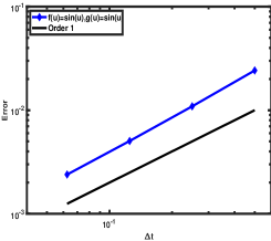
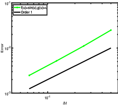
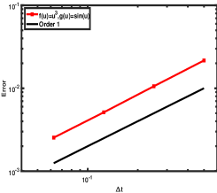
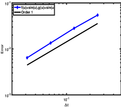
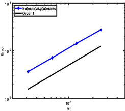
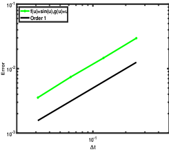
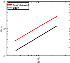
From Theorem 3.1 3.6 3.7 f ( u ) = sin ( u ) , g ( u ) = sin ( u ) formulae-sequence 𝑓 𝑢 𝑢 𝑔 𝑢 𝑢 f(u)=\sin(u),g(u)=\sin(u) f ( u ) = sin ( u ) , g ( u ) = u formulae-sequence 𝑓 𝑢 𝑢 𝑔 𝑢 𝑢 f(u)=\sin(u),g(u)=u f ( u ) = u 3 , g ( u ) = sin ( u ) . formulae-sequence 𝑓 𝑢 superscript 𝑢 3 𝑔 𝑢 𝑢 f(u)=u^{3},g(u)=\sin(u). { e k } k ∈ ℕ + subscript subscript 𝑒 𝑘 𝑘 limit-from ℕ \left\{e_{k}\right\}_{k\in\mathbb{N}+} { q k } k ∈ ℕ + subscript subscript 𝑞 𝑘 𝑘 limit-from ℕ \left\{q_{k}\right\}_{k\in\mathbb{N}+} Q 𝑄 Q e k = 2 4 sin ( k π x ) subscript 𝑒 𝑘 2 4 𝑘 𝜋 𝑥 e_{k}=\frac{\sqrt{2}}{4}\sin(k\pi x) q k = 1 k 6 subscript 𝑞 𝑘 1 superscript 𝑘 6 q_{k}=\frac{1}{k^{6}} x ∈ ( − 8 , 8 ) , 𝑥 8 8 x\in(-8,8), u ( 0 ) = 0 , 𝑢 0 0 u(0)=0, u t ( 0 ) = s e c h ( x ) , subscript 𝑢 𝑡 0 𝑠 𝑒 𝑐 ℎ 𝑥 u_{t}(0)=sech(x), u x ( 0 ) = 0 . subscript 𝑢 𝑥 0 0 u_{x}(0)=0. φ ( x ) = 1 / 1 + ‖ x ‖ 2 𝜑 𝑥 1 1 superscript norm 𝑥 2 \varphi(x)=1/\sqrt{1+\|x\|^{2}} c = 1 𝑐 1 c=1 n i = 5 subscript 𝑛 𝑖 5 n_{i}=5 1 Δ t = 2 − s , s = 1 , 2 , 3 , 4 , formulae-sequence Δ 𝑡 superscript 2 𝑠 𝑠 1 2 3 4
\Delta t=2^{-s},s=1,2,3,4, T = 1 𝑇 1 T=1 Δ t = 2 − 10 , Δ x = 2 − 5 formulae-sequence Δ 𝑡 superscript 2 10 Δ 𝑥 superscript 2 5 \Delta t=2^{-10},\Delta x=2^{-5} 1
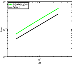
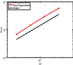
Table 1: Mean-square errors of LRBF collocation midpoint method in time.
Figure 1: Mean-square convergence order of LRBF collocation midpoint method in temporal direction in the cases of (1) f ( u ) = sin ( u ) , g ( u ) = sin ( u ) formulae-sequence 𝑓 𝑢 𝑢 𝑔 𝑢 𝑢 f(u)=\sin(u),g(u)=\sin(u) f ( u ) = sin ( u ) , g ( u ) = u formulae-sequence 𝑓 𝑢 𝑢 𝑔 𝑢 𝑢 f(u)=\sin(u),g(u)=u f ( u ) = u 3 , g ( u ) = sin ( u ) . formulae-sequence 𝑓 𝑢 superscript 𝑢 3 𝑔 𝑢 𝑢 f(u)=u^{3},g(u)=\sin(u).
Remark 3.2 .
By using (3.6 2.3
{ 𝐏 n + 1 − 𝐏 n Δ t = − 𝐃 ( 1 ) 𝓦 n + 1 2 − ( ( 𝐏 n + 1 2 ) 2 + ( 𝐐 n + 1 2 ) 2 ) 𝐐 n + 1 2 + 𝐐 n + 1 2 Δ 𝐖 n Δ t , 𝐐 n + 1 − 𝐐 n Δ t = 𝐃 ( 1 ) 𝐕 n + 1 2 + ( ( 𝐏 n + 1 2 ) 2 + ( 𝐐 n + 1 2 ) 2 ) 𝐏 n + 1 2 − 𝐏 n + 1 2 Δ 𝐖 n Δ t , 𝐃 ( 1 ) 𝐏 n + 1 2 = 𝐕 n + 1 2 , 𝐃 ( 1 ) 𝐐 n + 1 2 = 𝓦 n + 1 2 , \left\{\begin{aligned} &\frac{\mathbf{P}^{n+1}-\mathbf{P}^{n}}{\Delta t}=-\mathbf{D}^{(1)}\boldsymbol{\mathcal{W}}^{n+\frac{1}{2}}-\left((\mathbf{P}^{n+\frac{1}{2}})^{2}+(\mathbf{Q}^{n+\frac{1}{2}})^{2}\right)\mathbf{Q}^{n+\frac{1}{2}}+\mathbf{Q}^{n+\frac{1}{2}}\frac{\Delta\mathbf{W}^{n}}{\Delta t},\\
&\frac{\mathbf{Q}^{n+1}-\mathbf{Q}^{n}}{\Delta t}=\mathbf{D}^{(1)}\mathbf{V}^{n+\frac{1}{2}}+\left((\mathbf{P}^{n+\frac{1}{2}})^{2}+(\mathbf{Q}^{n+\frac{1}{2}})^{2}\right)\mathbf{P}^{n+\frac{1}{2}}-\mathbf{P}^{n+\frac{1}{2}}\frac{\Delta\mathbf{W}^{n}}{\Delta t},\\
&\mathbf{D}^{(1)}\mathbf{P}^{n+\frac{1}{2}}=\mathbf{V}^{n+\frac{1}{2}},\\
&\mathbf{D}^{(1)}\mathbf{Q}^{n+\frac{1}{2}}=\boldsymbol{\mathcal{W}}^{n+\frac{1}{2}},\end{aligned}\right. (3.10)
where P i n + 1 2 = P i n + P i n + 1 2 , subscript superscript 𝑃 𝑛 1 2 𝑖 subscript superscript 𝑃 𝑛 𝑖 subscript superscript 𝑃 𝑛 1 𝑖 2 P^{n+\frac{1}{2}}_{i}=\frac{P^{n}_{i}+P^{n+1}_{i}}{2}, Q i n + 1 2 = Q i n + Q i n + 1 2 , subscript superscript 𝑄 𝑛 1 2 𝑖 subscript superscript 𝑄 𝑛 𝑖 subscript superscript 𝑄 𝑛 1 𝑖 2 Q^{n+\frac{1}{2}}_{i}=\frac{Q^{n}_{i}+Q^{n+1}_{i}}{2}, i = 1 , … , I − 1 , 𝑖 1 … 𝐼 1
i=1,\dots,I-1,
( ( 𝐏 n + 1 2 ) 2 + ( 𝐐 n + 1 2 ) 2 ) 𝐐 n + 1 2 = [ ( ( P 1 n + 1 2 ) 2 + ( Q 1 n + 1 2 ) 2 ) Q 1 n + 1 2 , … , ( ( P I − 1 n + 1 2 ) 2 + ( Q I − 1 n + 1 2 ) 2 ) Q I − 1 n + 1 2 ] ⊤ , superscript superscript 𝐏 𝑛 1 2 2 superscript superscript 𝐐 𝑛 1 2 2 superscript 𝐐 𝑛 1 2 superscript superscript superscript subscript 𝑃 1 𝑛 1 2 2 superscript superscript subscript 𝑄 1 𝑛 1 2 2 superscript subscript 𝑄 1 𝑛 1 2 … superscript superscript subscript 𝑃 𝐼 1 𝑛 1 2 2 superscript superscript subscript 𝑄 𝐼 1 𝑛 1 2 2 superscript subscript 𝑄 𝐼 1 𝑛 1 2
top \displaystyle\left((\mathbf{P}^{n+\frac{1}{2}})^{2}+(\mathbf{Q}^{n+\frac{1}{2}})^{2}\right)\mathbf{Q}^{n+\frac{1}{2}}=\left[\left((P_{1}^{n+\frac{1}{2}})^{2}+(Q_{1}^{n+\frac{1}{2}})^{2}\right)Q_{1}^{n+\frac{1}{2}},\dots,\left((P_{I-1}^{n+\frac{1}{2}})^{2}+(Q_{I-1}^{n+\frac{1}{2}})^{2}\right)Q_{I-1}^{n+\frac{1}{2}}\right]^{\top},
( ( 𝐏 n + 1 2 ) 2 + ( 𝐐 n + 1 2 ) 2 ) 𝐏 n + 1 2 = [ ( ( P 1 n + 1 2 ) 2 + ( Q 1 n + 1 2 ) 2 ) P 1 n + 1 2 , … , ( ( P I − 1 n + 1 2 ) 2 + ( Q I − 1 n + 1 2 ) 2 ) P I − 1 n + 1 2 ] ⊤ , superscript superscript 𝐏 𝑛 1 2 2 superscript superscript 𝐐 𝑛 1 2 2 superscript 𝐏 𝑛 1 2 superscript superscript superscript subscript 𝑃 1 𝑛 1 2 2 superscript superscript subscript 𝑄 1 𝑛 1 2 2 superscript subscript 𝑃 1 𝑛 1 2 … superscript superscript subscript 𝑃 𝐼 1 𝑛 1 2 2 superscript superscript subscript 𝑄 𝐼 1 𝑛 1 2 2 superscript subscript 𝑃 𝐼 1 𝑛 1 2
top \displaystyle\left((\mathbf{P}^{n+\frac{1}{2}})^{2}+(\mathbf{Q}^{n+\frac{1}{2}})^{2}\right)\mathbf{P}^{n+\frac{1}{2}}=\left[\left((P_{1}^{n+\frac{1}{2}})^{2}+(Q_{1}^{n+\frac{1}{2}})^{2}\right)P_{1}^{n+\frac{1}{2}},\dots,\left((P_{I-1}^{n+\frac{1}{2}})^{2}+(Q_{I-1}^{n+\frac{1}{2}})^{2}\right)P_{I-1}^{n+\frac{1}{2}}\right]^{\top},
𝐐 n + 1 2 Δ 𝐖 n = [ Q 1 n + 1 2 ( W ( x 1 , t n + 1 ) − W ( x 1 , t n ) ) , … , Q I − 1 n + 1 2 ( W ( x I − 1 , t n + 1 ) − W ( x I − 1 , t n ) ) ] ⊤ , superscript 𝐐 𝑛 1 2 Δ superscript 𝐖 𝑛 superscript superscript subscript 𝑄 1 𝑛 1 2 𝑊 subscript 𝑥 1 subscript 𝑡 𝑛 1 𝑊 subscript 𝑥 1 subscript 𝑡 𝑛 … superscript subscript 𝑄 𝐼 1 𝑛 1 2 𝑊 subscript 𝑥 𝐼 1 subscript 𝑡 𝑛 1 𝑊 subscript 𝑥 𝐼 1 subscript 𝑡 𝑛
top \displaystyle\mathbf{Q}^{n+\frac{1}{2}}\Delta\mathbf{W}^{n}=[Q_{1}^{n+\frac{1}{2}}(W(x_{1},t_{n+1})-W(x_{1},t_{n})),\dots,Q_{I-1}^{n+\frac{1}{2}}(W(x_{I-1},t_{n+1})-W(x_{I-1},t_{n}))]^{\top},
𝐏 n + 1 2 Δ 𝐖 n = [ P 1 n + 1 2 ( W ( x 1 , t n + 1 ) − W ( x 1 , t n ) ) , … , P I − 1 n + 1 2 ( W ( x I − 1 , t n + 1 ) − W ( x I − 1 , t n ) ) ] ⊤ . superscript 𝐏 𝑛 1 2 Δ superscript 𝐖 𝑛 superscript superscript subscript 𝑃 1 𝑛 1 2 𝑊 subscript 𝑥 1 subscript 𝑡 𝑛 1 𝑊 subscript 𝑥 1 subscript 𝑡 𝑛 … superscript subscript 𝑃 𝐼 1 𝑛 1 2 𝑊 subscript 𝑥 𝐼 1 subscript 𝑡 𝑛 1 𝑊 subscript 𝑥 𝐼 1 subscript 𝑡 𝑛
top \displaystyle\mathbf{P}^{n+\frac{1}{2}}\Delta\mathbf{W}^{n}=[P_{1}^{n+\frac{1}{2}}(W(x_{1},t_{n+1})-W(x_{1},t_{n})),\dots,P_{I-1}^{n+\frac{1}{2}}(W(x_{I-1},t_{n+1})-W(x_{I-1},t_{n}))]^{\top}.
Similar to Theorem 3.1 3.10
ω i n + 1 − ω i n Δ t + ∑ k = 1 n i d k ( 1 ) i κ k n + 1 2 i = 0 , superscript subscript 𝜔 𝑖 𝑛 1 superscript subscript 𝜔 𝑖 𝑛 Δ 𝑡 superscript subscript 𝑘 1 subscript 𝑛 𝑖 subscript superscript subscript 𝑑 𝑘 1 𝑖 subscript subscript superscript 𝜅 𝑛 1 2 𝑘 𝑖 0 \frac{\omega_{i}^{n+1}-\omega_{i}^{n}}{\Delta t}+\sum_{k=1}^{n_{i}}{}_{i}d_{k}^{(1)}{}_{i}\kappa^{n+\frac{1}{2}}_{k}=0, (3.11)
where
ω i n = 1 2 d Z i n ∧ M d Z i n , κ k n + 1 2 i = d Z i n + 1 2 ∧ K d Z k n + 1 2 i , Z i n = ( P i n , Q i n , V i n , 𝒲 i n ) ⊤ , formulae-sequence superscript subscript 𝜔 𝑖 𝑛 1 2 d superscript subscript 𝑍 𝑖 𝑛 𝑀 d superscript subscript 𝑍 𝑖 𝑛 formulae-sequence subscript superscript subscript 𝜅 𝑘 𝑛 1 2 𝑖 d superscript subscript 𝑍 𝑖 𝑛 1 2 𝐾 d subscript superscript subscript 𝑍 𝑘 𝑛 1 2 𝑖 superscript subscript 𝑍 𝑖 𝑛 superscript superscript subscript 𝑃 𝑖 𝑛 superscript subscript 𝑄 𝑖 𝑛 superscript subscript 𝑉 𝑖 𝑛 superscript subscript 𝒲 𝑖 𝑛 top \displaystyle\omega_{i}^{n}=\frac{1}{2}\mathrm{d}Z_{i}^{n}\wedge M\mathrm{d}Z_{i}^{n},\quad{}_{i}\kappa_{k}^{n+\frac{1}{2}}=\mathrm{d}Z_{i}^{n+\frac{1}{2}}\wedge K\mathrm{d}{}_{i}Z_{k}^{n+\frac{1}{2}},\quad Z_{i}^{n}=(P_{i}^{n},Q_{i}^{n},V_{i}^{n},\mathcal{W}_{i}^{n})^{\top},
Z k n + 1 2 i = ( ( i P k n + i P k n + 1 ) / 2 , ( i Q k n + i Q k n + 1 ) / 2 , ( i V k n + i V k n + 1 ) / 2 , ( i 𝒲 k n + i 𝒲 k n + 1 ) / 2 ) ⊤ {}_{i}Z_{k}^{n+\frac{1}{2}}=\left((_{i}P_{k}^{n}+_{i}P_{k}^{n+1})/2,(_{i}Q_{k}^{n}+_{i}Q_{k}^{n+1})/2,(_{i}V_{k}^{n}+_{i}V_{k}^{n+1})/2,(_{i}\mathcal{W}_{k}^{n}+_{i}\mathcal{W}_{k}^{n+1})/2\right)^{\top}
with i = 1 , … , I − 1 𝑖 1 … 𝐼 1
i=1,\dots,I-1 k = 1 , … , n i , 𝑘 1 … subscript 𝑛 𝑖
k=1,\dots,n_{i},
M = ( 0 − 1 0 0 1 0 0 0 0 0 0 0 0 0 0 0 ) , K = ( 0 0 1 0 0 0 0 1 − 1 0 0 0 0 − 1 0 0 ) . formulae-sequence 𝑀 0 1 0 0 1 0 0 0 0 0 0 0 0 0 0 0 𝐾 0 0 1 0 0 0 0 1 1 0 0 0 0 1 0 0 \displaystyle M=\left(\begin{array}[]{cccc}0&-1&0&0\\
1&0&0&0\\
0&0&0&0\\
0&0&0&0\\
\end{array}\right),\quad K=\left(\begin{array}[]{cccc}0&0&1&0\\
0&0&0&1\\
-1&0&0&0\\
0&-1&0&0\\
\end{array}\right).
Remark 3.3 .
For the stochastic KdV equation (2.4 3.6
{ 1 2 𝐔 n + 1 − 𝐔 n Δ t + 𝐃 ( 1 ) 𝐕 n + 1 2 = λ Δ 𝐖 n Δ t , 1 2 𝓟 n + 1 − 𝓟 n Δ t + β 𝐃 ( 1 ) 𝓦 n + 1 2 = 𝐕 n + 1 2 − 1 2 ( 𝐔 n + 1 2 ) 2 , β 𝐃 ( 1 ) 𝐔 n + 1 2 = β 𝓦 n + 1 2 , − 𝐃 ( 1 ) 𝓟 n + 1 2 = − 𝐔 n + 1 2 , \left\{\begin{aligned} &\frac{1}{2}\frac{\mathbf{U}^{n+1}-\mathbf{U}^{n}}{\Delta t}+\mathbf{D}^{(1)}\mathbf{V}^{n+\frac{1}{2}}=\lambda\frac{\Delta\mathbf{W}^{n}}{\Delta t},\\
&\frac{1}{2}\frac{\boldsymbol{\mathcal{P}}^{n+1}-\boldsymbol{\mathcal{P}}^{n}}{\Delta t}+\beta\mathbf{D}^{(1)}\boldsymbol{\mathcal{W}}^{n+\frac{1}{2}}=\mathbf{V}^{n+\frac{1}{2}}-\frac{1}{2}(\mathbf{U}^{n+\frac{1}{2}})^{2},\\
&\beta\mathbf{D}^{(1)}\mathbf{U}^{n+\frac{1}{2}}=\beta\boldsymbol{\mathcal{W}}^{n+\frac{1}{2}},\\
&-\mathbf{D}^{(1)}\boldsymbol{\mathcal{P}}^{n+\frac{1}{2}}=-\mathbf{U}^{n+\frac{1}{2}},\end{aligned}\right. (3.12)
where U i n + 1 2 = U i n + U i n + 1 2 subscript superscript 𝑈 𝑛 1 2 𝑖 subscript superscript 𝑈 𝑛 𝑖 subscript superscript 𝑈 𝑛 1 𝑖 2 U^{n+\frac{1}{2}}_{i}=\frac{U^{n}_{i}+U^{n+1}_{i}}{2} V i n + 1 2 = V i n + V i n + 1 2 subscript superscript 𝑉 𝑛 1 2 𝑖 subscript superscript 𝑉 𝑛 𝑖 subscript superscript 𝑉 𝑛 1 𝑖 2 V^{n+\frac{1}{2}}_{i}=\frac{V^{n}_{i}+V^{n+1}_{i}}{2} 𝒫 i n + 1 2 = 𝒫 i n + 𝒫 i n + 1 2 subscript superscript 𝒫 𝑛 1 2 𝑖 subscript superscript 𝒫 𝑛 𝑖 subscript superscript 𝒫 𝑛 1 𝑖 2 \mathcal{P}^{n+\frac{1}{2}}_{i}=\frac{\mathcal{P}^{n}_{i}+\mathcal{P}^{n+1}_{i}}{2} 𝒲 i n + 1 2 = 𝒲 i n + 𝒲 i n + 1 2 subscript superscript 𝒲 𝑛 1 2 𝑖 subscript superscript 𝒲 𝑛 𝑖 subscript superscript 𝒲 𝑛 1 𝑖 2 \mathcal{W}^{n+\frac{1}{2}}_{i}=\frac{\mathcal{W}^{n}_{i}+\mathcal{W}^{n+1}_{i}}{2} i = 1 , … , I − 1 𝑖 1 … 𝐼 1
i=1,\dots,I-1
( 𝐔 n + 1 2 ) 2 = [ ( U 1 n + 1 2 ) 2 , … , ( U I − 1 n + 1 2 ) 2 ] ⊤ , Δ 𝐖 n = [ W ( x 1 , t n + 1 ) − W ( x 1 , t n ) , … , W ( x I − 1 , t n + 1 ) − W ( x I − 1 , t n ) ] ⊤ . formulae-sequence superscript superscript 𝐔 𝑛 1 2 2 superscript superscript superscript subscript 𝑈 1 𝑛 1 2 2 … superscript superscript subscript 𝑈 𝐼 1 𝑛 1 2 2
top Δ superscript 𝐖 𝑛 superscript 𝑊 subscript 𝑥 1 subscript 𝑡 𝑛 1 𝑊 subscript 𝑥 1 subscript 𝑡 𝑛 … 𝑊 subscript 𝑥 𝐼 1 subscript 𝑡 𝑛 1 𝑊 subscript 𝑥 𝐼 1 subscript 𝑡 𝑛
top (\mathbf{U}^{n+\frac{1}{2}})^{2}=[(U_{1}^{n+\frac{1}{2}})^{2},\dots,(U_{I-1}^{n+\frac{1}{2}})^{2}]^{\top},\Delta\mathbf{W}^{n}=[W(x_{1},t_{n+1})-W(x_{1},t_{n}),\dots,W(x_{I-1},t_{n+1})-W(x_{I-1},t_{n})]^{\top}.
In fact, the fully-discrete method (3.12
ω i n + 1 − ω i n Δ t + ∑ k = 1 n i d k ( 1 ) i κ k n + 1 2 i = 0 , i = 1 , … , I − 1 formulae-sequence superscript subscript 𝜔 𝑖 𝑛 1 superscript subscript 𝜔 𝑖 𝑛 Δ 𝑡 superscript subscript 𝑘 1 subscript 𝑛 𝑖 subscript superscript subscript 𝑑 𝑘 1 𝑖 subscript subscript superscript 𝜅 𝑛 1 2 𝑘 𝑖 0 𝑖 1 … 𝐼 1
\frac{\omega_{i}^{n+1}-\omega_{i}^{n}}{\Delta t}+\sum_{k=1}^{n_{i}}{}_{i}d_{k}^{(1)}{}_{i}\kappa^{n+\frac{1}{2}}_{k}=0,\qquad i=1,\dots,I-1 (3.13)
with
ω i n = 1 2 d Z i n ∧ M d Z i n , κ k n + 1 2 i = d Z i n + 1 2 ∧ K d Z k n + 1 2 i , Z i n = ( U i n , V i n , 𝒫 i n , 𝒲 i n ) ⊤ , formulae-sequence superscript subscript 𝜔 𝑖 𝑛 1 2 d superscript subscript 𝑍 𝑖 𝑛 𝑀 d superscript subscript 𝑍 𝑖 𝑛 formulae-sequence subscript superscript subscript 𝜅 𝑘 𝑛 1 2 𝑖 d superscript subscript 𝑍 𝑖 𝑛 1 2 𝐾 d subscript superscript subscript 𝑍 𝑘 𝑛 1 2 𝑖 superscript subscript 𝑍 𝑖 𝑛 superscript superscript subscript 𝑈 𝑖 𝑛 superscript subscript 𝑉 𝑖 𝑛 superscript subscript 𝒫 𝑖 𝑛 superscript subscript 𝒲 𝑖 𝑛 top \displaystyle\omega_{i}^{n}=\frac{1}{2}\mathrm{d}Z_{i}^{n}\wedge M\mathrm{d}Z_{i}^{n},\quad{}_{i}\kappa_{k}^{n+\frac{1}{2}}=\mathrm{d}Z_{i}^{n+\frac{1}{2}}\wedge K\mathrm{d}{}_{i}Z_{k}^{n+\frac{1}{2}},\quad Z_{i}^{n}=(U_{i}^{n},V_{i}^{n},\mathcal{P}_{i}^{n},\mathcal{W}_{i}^{n})^{\top},
Z k n + 1 2 i = ( ( i U k n + i U k n + 1 ) / 2 , ( i V k n + i V k n + 1 ) / 2 , ( i 𝒫 k n + i 𝒫 k n + 1 ) / 2 , ( i 𝒲 k n + i 𝒲 k n + 1 ) / 2 ) ⊤ , {}_{i}Z_{k}^{n+\frac{1}{2}}=\left((_{i}U_{k}^{n}+_{i}U_{k}^{n+1})/2,(_{i}V_{k}^{n}+_{i}V_{k}^{n+1})/2,(_{i}\mathcal{P}_{k}^{n}+_{i}\mathcal{P}_{k}^{n+1})/2,(_{i}\mathcal{W}_{k}^{n}+_{i}\mathcal{W}_{k}^{n+1})/2\right)^{\top},
and
M = ( 0 0 − 1 2 0 0 0 0 0 1 2 0 0 0 0 0 0 0 ) , K = ( 0 0 0 − β 0 0 − 1 0 0 1 0 0 β 0 0 0 ) . formulae-sequence 𝑀 0 0 1 2 0 0 0 0 0 1 2 0 0 0 0 0 0 0 𝐾 0 0 0 𝛽 0 0 1 0 0 1 0 0 𝛽 0 0 0 \displaystyle M=\left(\begin{array}[]{cccc}0&0&-\frac{1}{2}&0\\
0&0&0&0\\
\frac{1}{2}&0&0&0\\
0&0&0&0\\
\end{array}\right),\quad K=\left(\begin{array}[]{cccc}0&0&0&-\beta\\
0&0&-1&0\\
0&1&0&0\\
\beta&0&0&0\\
\end{array}\right).
Remark 3.4 .
For the stochastic Maxwell equation (2.5 3.6
{ ( 𝐄 1 ) n + 1 − ( 𝐄 1 ) n Δ t = − 𝐃 z ( 1 ) ( 𝐇 2 ) n + 1 2 + 𝐃 y ( 1 ) ( 𝐇 3 ) n + 1 2 − λ ( 𝐇 1 ) n + 1 2 Δ 𝐖 n Δ t , ( 𝐄 2 ) n + 1 − ( 𝐄 2 ) n Δ t = 𝐃 z ( 1 ) ( 𝐇 1 ) n + 1 2 − 𝐃 x ( 1 ) ( 𝐇 3 ) n + 1 2 − λ ( 𝐇 2 ) n + 1 2 Δ 𝐖 n Δ t , ( 𝐄 3 ) n + 1 − ( 𝐄 3 ) n Δ t = − 𝐃 y ( 1 ) ( 𝐇 1 ) n + 1 2 + 𝐃 x ( 1 ) ( 𝐇 2 ) n + 1 2 − λ ( 𝐇 3 ) n + 1 2 Δ 𝐖 n Δ t , ( 𝐇 1 ) n + 1 − ( 𝐇 1 ) n Δ t = 𝐃 z ( 1 ) ( 𝐄 2 ) n + 1 2 − 𝐃 y ( 1 ) ( 𝐄 3 ) n + 1 2 + λ ( 𝐄 1 ) n + 1 2 Δ 𝐖 n Δ t , ( 𝐇 2 ) n + 1 − ( 𝐇 2 ) n Δ t = − 𝐃 z ( 1 ) ( 𝐄 1 ) n + 1 2 + 𝐃 x ( 1 ) ( 𝐄 3 ) n + 1 2 + λ ( 𝐄 2 ) n + 1 2 Δ 𝐖 n Δ t , ( 𝐇 3 ) n + 1 − ( 𝐇 3 ) n Δ t = 𝐃 y ( 1 ) ( 𝐄 1 ) n + 1 2 − 𝐃 x ( 1 ) ( 𝐄 2 ) n + 1 2 + λ ( 𝐄 3 ) n + 1 2 Δ 𝐖 n Δ t , \left\{\begin{aligned} &\frac{(\mathbf{E}_{1})^{n+1}-(\mathbf{E}_{1})^{n}}{\Delta t}=-\mathbf{D}_{z}^{(1)}(\mathbf{H}_{2})^{n+\frac{1}{2}}+\mathbf{D}_{y}^{(1)}(\mathbf{H}_{3})^{n+\frac{1}{2}}-\lambda(\mathbf{H}_{1})^{n+\frac{1}{2}}\frac{\Delta\mathbf{W}^{n}}{\Delta t},\\
&\frac{(\mathbf{E}_{2})^{n+1}-(\mathbf{E}_{2})^{n}}{\Delta t}=~{}\mathbf{D}_{z}^{(1)}(\mathbf{H}_{1})^{n+\frac{1}{2}}-\mathbf{D}_{x}^{(1)}(\mathbf{H}_{3})^{n+\frac{1}{2}}-\lambda(\mathbf{H}_{2})^{n+\frac{1}{2}}\frac{\Delta\mathbf{W}^{n}}{\Delta t},\\
&\frac{(\mathbf{E}_{3})^{n+1}-(\mathbf{E}_{3})^{n}}{\Delta t}=-\mathbf{D}_{y}^{(1)}(\mathbf{H}_{1})^{n+\frac{1}{2}}+\mathbf{D}_{x}^{(1)}(\mathbf{H}_{2})^{n+\frac{1}{2}}-\lambda(\mathbf{H}_{3})^{n+\frac{1}{2}}\frac{\Delta\mathbf{W}^{n}}{\Delta t},\\
&\frac{(\mathbf{H}_{1})^{n+1}-(\mathbf{H}_{1})^{n}}{\Delta t}=~{}\mathbf{D}_{z}^{(1)}(\mathbf{E}_{2})^{n+\frac{1}{2}}-\mathbf{D}_{y}^{(1)}(\mathbf{E}_{3})^{n+\frac{1}{2}}+\lambda(\mathbf{E}_{1})^{n+\frac{1}{2}}\frac{\Delta\mathbf{W}^{n}}{\Delta t},\\
&\frac{(\mathbf{H}_{2})^{n+1}-(\mathbf{H}_{2})^{n}}{\Delta t}=-\mathbf{D}_{z}^{(1)}(\mathbf{E}_{1})^{n+\frac{1}{2}}+\mathbf{D}_{x}^{(1)}(\mathbf{E}_{3})^{n+\frac{1}{2}}+\lambda(\mathbf{E}_{2})^{n+\frac{1}{2}}\frac{\Delta\mathbf{W}^{n}}{\Delta t},\\
&\frac{(\mathbf{H}_{3})^{n+1}-(\mathbf{H}_{3})^{n}}{\Delta t}=~{}\mathbf{D}_{y}^{(1)}(\mathbf{E}_{1})^{n+\frac{1}{2}}-\mathbf{D}_{x}^{(1)}(\mathbf{E}_{2})^{n+\frac{1}{2}}+\lambda(\mathbf{E}_{3})^{n+\frac{1}{2}}\frac{\Delta\mathbf{W}^{n}}{\Delta t},\end{aligned}\right. (3.14)
where
( 𝐄 j ) n + 1 2 = ( ( 𝐄 j ) n + 1 + ( 𝐄 j ) n ) / 2 , ( 𝐇 j ) n + 1 2 = ( ( 𝐇 j ) n + 1 + ( 𝐇 j ) n ) / 2 , formulae-sequence superscript subscript 𝐄 𝑗 𝑛 1 2 superscript subscript 𝐄 𝑗 𝑛 1 superscript subscript 𝐄 𝑗 𝑛 2 superscript subscript 𝐇 𝑗 𝑛 1 2 superscript subscript 𝐇 𝑗 𝑛 1 superscript subscript 𝐇 𝑗 𝑛 2 \displaystyle(\mathbf{E}_{j})^{n+\frac{1}{2}}=((\mathbf{E}_{j})^{n+1}+(\mathbf{E}_{j})^{n})/2,\quad(\mathbf{H}_{j})^{n+\frac{1}{2}}=((\mathbf{H}_{j})^{n+1}+(\mathbf{H}_{j})^{n})/2,
( 𝐄 j ) n = [ ( E j ) 1 n , … , ( E j ) I − 1 n ] ⊤ , ( 𝐇 j ) n = [ ( H j ) 1 n , … , ( H j ) I − 1 n ] ⊤ , j = 1 , 2 , 3 , formulae-sequence superscript subscript 𝐄 𝑗 𝑛 superscript superscript subscript subscript 𝐸 𝑗 1 𝑛 … superscript subscript subscript 𝐸 𝑗 𝐼 1 𝑛
top formulae-sequence superscript subscript 𝐇 𝑗 𝑛 superscript superscript subscript subscript 𝐻 𝑗 1 𝑛 … superscript subscript subscript 𝐻 𝑗 𝐼 1 𝑛
top 𝑗 1 2 3
\displaystyle(\mathbf{E}_{j})^{n}=[(E_{j})_{1}^{n},\dots,(E_{j})_{I-1}^{n}]^{\top},\quad~{}(\mathbf{H}_{j})^{n}=[(H_{j})_{1}^{n},\dots,(H_{j})_{I-1}^{n}]^{\top},\quad j=1,2,3,
Δ 𝐖 n = [ W ( x 1 , t n + 1 ) − W ( x 1 , t n ) , … , W ( x I − 1 , t n + 1 ) − W ( x I − 1 , t n ) ] ⊤ . Δ superscript 𝐖 𝑛 superscript 𝑊 subscript 𝑥 1 subscript 𝑡 𝑛 1 𝑊 subscript 𝑥 1 subscript 𝑡 𝑛 … 𝑊 subscript 𝑥 𝐼 1 subscript 𝑡 𝑛 1 𝑊 subscript 𝑥 𝐼 1 subscript 𝑡 𝑛
top \displaystyle\Delta\mathbf{W}^{n}=[W(x_{1},t_{n+1})-W(x_{1},t_{n}),\dots,W(x_{I-1},t_{n+1})-W(x_{I-1},t_{n})]^{\top}.
In the three-dimensional case, 𝐃 x ( 1 ) , superscript subscript 𝐃 𝑥 1 \mathbf{D}_{x}^{(1)}, 𝐃 y ( 1 ) superscript subscript 𝐃 𝑦 1 \mathbf{D}_{y}^{(1)} 𝐃 z ( 1 ) superscript subscript 𝐃 𝑧 1 \mathbf{D}_{z}^{(1)} 1 1 1 ∂ x 𝑥 \partial x ∂ y 𝑦 \partial y ∂ z 𝑧 \partial z 3.4 d x , k ( 1 ) i , d y , k ( 1 ) i , d z , k ( 1 ) i subscript superscript subscript 𝑑 𝑥 𝑘
1 𝑖 subscript superscript subscript 𝑑 𝑦 𝑘
1 𝑖 subscript superscript subscript 𝑑 𝑧 𝑘
1 𝑖
{}_{i}d_{x,k}^{(1)},{}_{i}d_{y,k}^{(1)},{}_{i}d_{z,k}^{(1)} i ∈ { 1 , … , I − 1 } 𝑖 1 … 𝐼 1 i\in\{1,\dots,I-1\} k ∈ { 1 , … , n i } 𝑘 1 … subscript 𝑛 𝑖 k\in\{1,\dots,n_{i}\} 3.14
ω i n + 1 − ω i n Δ t + ∑ k = 1 n i d x , k ( 1 ) i κ 1 , k n + 1 2 i + ∑ k = 1 n i d y , k ( 1 ) i κ 2 , k n + 1 2 i + ∑ k = 1 n i d z , k ( 1 ) i κ 3 , k n + 1 2 i = 0 , i = 1 , … , I − 1 , formulae-sequence superscript subscript 𝜔 𝑖 𝑛 1 superscript subscript 𝜔 𝑖 𝑛 Δ 𝑡 superscript subscript 𝑘 1 subscript 𝑛 𝑖 subscript superscript subscript 𝑑 𝑥 𝑘
1 𝑖 subscript subscript superscript 𝜅 𝑛 1 2 1 𝑘
𝑖 superscript subscript 𝑘 1 subscript 𝑛 𝑖 subscript superscript subscript 𝑑 𝑦 𝑘
1 𝑖 subscript subscript superscript 𝜅 𝑛 1 2 2 𝑘
𝑖 superscript subscript 𝑘 1 subscript 𝑛 𝑖 subscript superscript subscript 𝑑 𝑧 𝑘
1 𝑖 subscript subscript superscript 𝜅 𝑛 1 2 3 𝑘
𝑖 0 𝑖 1 … 𝐼 1
\frac{\omega_{i}^{n+1}-\omega_{i}^{n}}{\Delta t}+\sum_{k=1}^{n_{i}}{}_{i}d_{x,k}^{(1)}{}_{i}\kappa^{n+\frac{1}{2}}_{1,k}+\sum_{k=1}^{n_{i}}{}_{i}d_{y,k}^{(1)}{}_{i}\kappa^{n+\frac{1}{2}}_{2,k}+\sum_{k=1}^{n_{i}}{}_{i}d_{z,k}^{(1)}{}_{i}\kappa^{n+\frac{1}{2}}_{3,k}=0,\qquad i=1,\dots,I-1, (3.15)
where
ω i n = 1 2 d Z i n ∧ M d Z i n , κ j , k n + 1 2 i = d Z i n + 1 2 ∧ K j d Z k n + 1 2 i , Z i n = ( ( H 1 ) i n , ( H 2 ) i n , ( H 3 ) i n , ( E 1 ) i n , ( E 2 ) i n , ( E 3 ) i n ) ⊤ , formulae-sequence superscript subscript 𝜔 𝑖 𝑛 1 2 d superscript subscript 𝑍 𝑖 𝑛 𝑀 d superscript subscript 𝑍 𝑖 𝑛 formulae-sequence subscript superscript subscript 𝜅 𝑗 𝑘
𝑛 1 2 𝑖 d superscript subscript 𝑍 𝑖 𝑛 1 2 subscript 𝐾 𝑗 d subscript superscript subscript 𝑍 𝑘 𝑛 1 2 𝑖 superscript subscript 𝑍 𝑖 𝑛 superscript superscript subscript subscript 𝐻 1 𝑖 𝑛 superscript subscript subscript 𝐻 2 𝑖 𝑛 superscript subscript subscript 𝐻 3 𝑖 𝑛 superscript subscript subscript 𝐸 1 𝑖 𝑛 superscript subscript subscript 𝐸 2 𝑖 𝑛 superscript subscript subscript 𝐸 3 𝑖 𝑛 top \displaystyle\omega_{i}^{n}=\frac{1}{2}\mathrm{d}Z_{i}^{n}\wedge M\mathrm{d}Z_{i}^{n},\quad{}_{i}\kappa_{j,k}^{n+\frac{1}{2}}=\mathrm{d}{}Z_{i}^{n+\frac{1}{2}}\wedge K_{j}\mathrm{d}{}_{i}Z_{k}^{n+\frac{1}{2}},\quad Z_{i}^{n}=((H_{1})_{i}^{n},(H_{2})_{i}^{n},(H_{3})_{i}^{n},(E_{1})_{i}^{n},(E_{2})_{i}^{n},(E_{3})_{i}^{n})^{\top},
Z k n + 1 2 i = ( ( i ( H 1 ) k n + i ( H 1 ) k n + 1 ) / 2 , ( i ( H 2 ) k n + i ( H 2 ) k n + 1 ) / 2 , ( i ( H 3 ) k n + i ( H 3 ) k n + 1 ) / 2 , ( i ( E 1 ) k n + i ( E 1 ) k n + 1 ) / 2 , {}_{i}Z_{k}^{n+\frac{1}{2}}=\left((_{i}(H_{1})_{k}^{n}+_{i}(H_{1})_{k}^{n+1})/2,(_{i}(H_{2})_{k}^{n}+_{i}(H_{2})_{k}^{n+1})/2,(_{i}(H_{3})_{k}^{n}+_{i}(H_{3})_{k}^{n+1})/2,(_{i}(E_{1})_{k}^{n}+_{i}(E_{1})_{k}^{n+1})/2,\right.
( i ( E 2 ) k n + i ( E 2 ) k n + 1 ) / 2 , ( i ( E 3 ) k n + i ( E 3 ) k n + 1 ) / 2 ) ⊤ , \displaystyle\left.~{}\qquad\qquad(_{i}(E_{2})_{k}^{n}+_{i}(E_{2})_{k}^{n+1})/2,(_{i}(E_{3})_{k}^{n}+_{i}(E_{3})_{k}^{n+1})/2\right)^{\top},
and
M = ( 0 − I 3 × 3 I 3 × 3 0 ) , K j = ( 𝒟 j 0 0 𝒟 j ) , j = 1 , 2 , 3 formulae-sequence 𝑀 0 subscript 𝐼 3 3 subscript 𝐼 3 3 0 formulae-sequence subscript 𝐾 𝑗 subscript 𝒟 𝑗 0 0 subscript 𝒟 𝑗 𝑗 1 2 3
M=\left(\begin{array}[]{cc}0&-I_{3\times 3}\\
I_{3\times 3}&0\end{array}\right),\quad K_{j}=\left(\begin{array}[]{cc}\mathscr{D}_{j}&0\\
0&\mathscr{D}_{j}\end{array}\right),\quad j=1,2,3
with I 3 × 3 subscript 𝐼 3 3 I_{3\times 3} 3 × 3 3 3 3\times 3
𝒟 1 = ( 0 0 0 0 0 − 1 0 1 0 ) , 𝒟 2 = ( 0 0 1 0 0 0 − 1 0 0 ) , 𝒟 3 = ( 0 − 1 0 1 0 0 0 0 0 ) . formulae-sequence subscript 𝒟 1 0 0 0 0 0 1 0 1 0 formulae-sequence subscript 𝒟 2 0 0 1 0 0 0 1 0 0 subscript 𝒟 3 0 1 0 1 0 0 0 0 0 \mathscr{D}_{1}=\left(\begin{array}[]{ccc}0&0&0\\
0&0&-1\\
0&1&0\end{array}\right),\quad\mathscr{D}_{2}=\left(\begin{array}[]{ccc}0&0&1\\
0&0&0\\
-1&0&0\end{array}\right),\quad\mathscr{D}_{3}=\left(\begin{array}[]{ccc}0&-1&0\\
1&0&0\\
0&0&0\end{array}\right).
4 Splitting multi-symplectic Runge–Kutta method
In this section, we propose the second kind of multi-symplectic methods for (2.1
Now we begin our study with the multi-symplectic Runge–Kutta method for deterministic Hamiltonian PDEs
M d z + K z x d t = ∇ S 1 ( z ) d t . 𝑀 𝑑 𝑧 𝐾 subscript 𝑧 𝑥 𝑑 𝑡 ∇ subscript 𝑆 1 𝑧 𝑑 𝑡 Mdz+Kz_{x}dt=\nabla S_{1}(z)dt. (4.1)
Applying s 𝑠 s r 𝑟 r ( c , A , b ) 𝑐 𝐴 𝑏 (c,A,b) ( c ~ , A ~ , b ~ ) ~ 𝑐 ~ 𝐴 ~ 𝑏 (\tilde{c},\tilde{A},\tilde{b})
c 1 a 11 … a 1 s ⋮ ⋮ ⋮ c s a s 1 … a s s b 1 … b s , c ~ 1 a ~ 11 … a ~ 1 r ⋮ ⋮ ⋮ c ~ r a ~ r 1 … a ~ r r b ~ 1 … b ~ r , subscript 𝑐 1 subscript 𝑎 11 … subscript 𝑎 1 𝑠 ⋮ ⋮ missing-subexpression ⋮ subscript 𝑐 𝑠 subscript 𝑎 𝑠 1 … subscript 𝑎 𝑠 𝑠 missing-subexpression missing-subexpression missing-subexpression missing-subexpression missing-subexpression subscript 𝑏 1 … subscript 𝑏 𝑠 subscript ~ 𝑐 1 subscript ~ 𝑎 11 … subscript ~ 𝑎 1 𝑟 ⋮ ⋮ missing-subexpression ⋮ subscript ~ 𝑐 𝑟 subscript ~ 𝑎 𝑟 1 … subscript ~ 𝑎 𝑟 𝑟 missing-subexpression missing-subexpression missing-subexpression missing-subexpression missing-subexpression subscript ~ 𝑏 1 … subscript ~ 𝑏 𝑟
\begin{array}[]{c|ccc}c_{1}&a_{11}&\dots&a_{1s}\\
\vdots&\vdots&&\vdots\\
c_{s}&a_{s1}&\dots&a_{ss}\\
\hline\cr&b_{1}&\dots&b_{s}\end{array},\qquad\begin{array}[]{c|ccc}\tilde{c}_{1}&\tilde{a}_{11}&\dots&\tilde{a}_{1r}\\
\vdots&\vdots&&\vdots\\
\tilde{c}_{r}&\tilde{a}_{r1}&\dots&\tilde{a}_{rr}\\
\hline\cr&\tilde{b}_{1}&\dots&\tilde{b}_{r}\end{array}, (4.2)
where s , r ≥ 1 , 𝑠 𝑟
1 s,r\geq 1, 4.1
Z m k = z i k + Δ x ∑ n = 1 s a m n δ x n , k Z n k , ∀ i = 0 , 1 , … , s , formulae-sequence superscript subscript 𝑍 𝑚 𝑘 superscript subscript 𝑧 𝑖 𝑘 Δ 𝑥 superscript subscript 𝑛 1 𝑠 subscript 𝑎 𝑚 𝑛 superscript subscript 𝛿 𝑥 𝑛 𝑘
superscript subscript 𝑍 𝑛 𝑘 for-all 𝑖 0 1 … 𝑠
\displaystyle Z_{m}^{k}=z_{i}^{k}+{\Delta x}\sum_{n=1}^{s}a_{mn}\delta_{x}^{n,k}Z_{n}^{k},\quad\forall~{}i=0,1,\ldots,s, (4.3)
z i + 1 k = z i k + Δ x ∑ m = 1 s b m δ x m , k Z m k , ∀ i = 0 , 1 , … , s , formulae-sequence superscript subscript 𝑧 𝑖 1 𝑘 superscript subscript 𝑧 𝑖 𝑘 Δ 𝑥 superscript subscript 𝑚 1 𝑠 subscript 𝑏 𝑚 superscript subscript 𝛿 𝑥 𝑚 𝑘
superscript subscript 𝑍 𝑚 𝑘 for-all 𝑖 0 1 … 𝑠
\displaystyle z_{i+1}^{k}=z_{i}^{k}+{\Delta x}\sum_{m=1}^{s}b_{m}\delta_{x}^{m,k}Z_{m}^{k},\quad\forall~{}i=0,1,\ldots,s,
Z m k = z m p + Δ t ∑ j = 1 r a ~ k j δ t m , j Z m j , ∀ p = 0 , 1 , … , r , formulae-sequence superscript subscript 𝑍 𝑚 𝑘 superscript subscript 𝑧 𝑚 𝑝 Δ 𝑡 superscript subscript 𝑗 1 𝑟 subscript ~ 𝑎 𝑘 𝑗 superscript subscript 𝛿 𝑡 𝑚 𝑗
superscript subscript 𝑍 𝑚 𝑗 for-all 𝑝 0 1 … 𝑟
\displaystyle Z_{m}^{k}=z_{m}^{p}+\Delta t\sum_{j=1}^{r}\tilde{a}_{kj}\delta_{t}^{m,j}Z_{m}^{j},\quad\forall~{}p=0,1,\ldots,r,
z m p + 1 = z m p + Δ t ∑ k = 1 r b ~ k δ t m , k Z m k , ∀ p = 0 , 1 , … , r , formulae-sequence superscript subscript 𝑧 𝑚 𝑝 1 superscript subscript 𝑧 𝑚 𝑝 Δ 𝑡 superscript subscript 𝑘 1 𝑟 subscript ~ 𝑏 𝑘 superscript subscript 𝛿 𝑡 𝑚 𝑘
superscript subscript 𝑍 𝑚 𝑘 for-all 𝑝 0 1 … 𝑟
\displaystyle z_{m}^{p+1}=z_{m}^{p}+\Delta t\sum_{k=1}^{r}\tilde{b}_{k}\delta_{t}^{m,k}Z_{m}^{k},\quad\forall~{}p=0,1,\ldots,r,
M δ t m , k Z m k + K δ x m , k Z m k = ∇ z S 1 ( Z m k ) , 𝑀 superscript subscript 𝛿 𝑡 𝑚 𝑘
superscript subscript 𝑍 𝑚 𝑘 𝐾 superscript subscript 𝛿 𝑥 𝑚 𝑘
superscript subscript 𝑍 𝑚 𝑘 subscript ∇ 𝑧 subscript 𝑆 1 superscript subscript 𝑍 𝑚 𝑘 \displaystyle M\delta_{t}^{m,k}Z_{m}^{k}+K\delta_{x}^{m,k}Z_{m}^{k}=\nabla_{z}S_{1}\left(Z_{m}^{k}\right),
where δ t m , k superscript subscript 𝛿 𝑡 𝑚 𝑘
\delta_{t}^{m,k} δ x m , k superscript subscript 𝛿 𝑥 𝑚 𝑘
\delta_{x}^{m,k} ∂ t subscript 𝑡 \partial_{t} ∂ x subscript 𝑥 \partial_{x}
b m b n − b m a m n − b n a n m = 0 and b ~ k b ~ j − b ~ k a ~ k j − b ~ j a ~ j k = 0 subscript 𝑏 𝑚 subscript 𝑏 𝑛 subscript 𝑏 𝑚 subscript 𝑎 𝑚 𝑛 subscript 𝑏 𝑛 subscript 𝑎 𝑛 𝑚 0 and subscript ~ 𝑏 𝑘 subscript ~ 𝑏 𝑗 subscript ~ 𝑏 𝑘 subscript ~ 𝑎 𝑘 𝑗 subscript ~ 𝑏 𝑗 subscript ~ 𝑎 𝑗 𝑘 0 \displaystyle b_{m}b_{n}-b_{m}a_{mn}-b_{n}a_{nm}=0\text{ and }\tilde{b}_{k}\tilde{b}_{j}-\tilde{b}_{k}\tilde{a}_{kj}-\tilde{b}_{j}\tilde{a}_{jk}=0 (4.4)
for all m , n = 1 , … , s formulae-sequence 𝑚 𝑛
1 … 𝑠
m,n=1,\ldots,s k , j = 1 , … , r formulae-sequence 𝑘 𝑗
1 … 𝑟
k,j=1,\ldots,r
ω p + 1 − ω p Δ t + κ i + 1 − κ i h = 0 , superscript 𝜔 𝑝 1 superscript 𝜔 𝑝 Δ 𝑡 subscript 𝜅 𝑖 1 subscript 𝜅 𝑖 ℎ 0 \displaystyle\frac{\omega^{p+1}-\omega^{p}}{\Delta t}+\frac{\kappa_{i+1}-\kappa_{i}}{h}=0,
where
ω p = 1 2 ∑ m = 1 s b m d z m p ∧ M d z m p , superscript 𝜔 𝑝 1 2 superscript subscript 𝑚 1 𝑠 subscript 𝑏 𝑚 d superscript subscript 𝑧 𝑚 𝑝 𝑀 d superscript subscript 𝑧 𝑚 𝑝 \omega^{p}=\frac{1}{2}\sum\limits_{m=1}^{s}b_{m}\mathrm{d}z_{m}^{p}\wedge M\mathrm{d}z_{m}^{p}, κ i = 1 2 ∑ k = 1 r b ~ k d z i k ∧ K d z i k subscript 𝜅 𝑖 1 2 superscript subscript 𝑘 1 𝑟 subscript ~ 𝑏 𝑘 d superscript subscript 𝑧 𝑖 𝑘 𝐾 d superscript subscript 𝑧 𝑖 𝑘 \kappa_{i}=\frac{1}{2}\sum\limits_{k=1}^{r}\tilde{b}_{k}\mathrm{d}z_{i}^{k}\wedge K\mathrm{d}z_{i}^{k} p = 0 , 1 , … , r 𝑝 0 1 … 𝑟
p=0,1,\ldots,r i = 0 , 1 , … , s . 𝑖 0 1 … 𝑠
i=0,1,\ldots,s. 2.1 t ∈ [ t m , t m + 1 ] 𝑡 subscript 𝑡 𝑚 subscript 𝑡 𝑚 1 t\in[t_{m},t_{m+1}]
{ M d z ¯ + K z ¯ x d t = ∇ S 1 ( z ¯ ) d t , z ¯ ( t m ) = z ( t m ) , and { K z x = 0 , M d z = ∇ S 2 ( z ) ∘ d W ( t ) , z ( t m ) = z ¯ ( t m + 1 ) . \left\{\begin{aligned} &Md\bar{z}+K\bar{z}_{x}dt=\nabla S_{1}(\bar{z})dt,\\
&\bar{z}(t_{m})=z(t_{m}),\end{aligned}\right.\qquad{\rm and}\qquad\left\{\begin{aligned} &Kz_{x}=0,\\
&Mdz=\nabla S_{2}(z)\circ dW(t),\\
&z(t_{m})=\overline{z}(t_{m+1}).\end{aligned}\right. (4.5)
By choosing symplectic methods for the stochastic system and combining (4.3
We first focus on the nonlinear stochastic wave equation (2.2 2.2 [ t 0 , t 1 ] subscript 𝑡 0 subscript 𝑡 1 [t_{0},t_{1}]
{ u ¯ t = v ¯ , u ¯ x = w ¯ , v ¯ t − w ¯ x = − f ( u ¯ ) , u ¯ ( t 0 ) = u ( t 0 ) , v ¯ ( t 0 ) = v ( t 0 ) , \left\{\begin{aligned} &\overline{u}_{t}=\overline{v},\\
&\overline{u}_{x}=\overline{w},\\
&\overline{v}_{t}-\overline{w}_{x}=-f(\overline{u}),\\
&\overline{u}(t_{0})=u(t_{0}),~{}\overline{v}(t_{0})=v(t_{0}),\end{aligned}\right. (4.6)
and a stochastic system
{ u x = 0 , w x = 0 , u t = 0 , d v = g ( u ) ∘ d W ( t ) , u ( t 0 ) = u ¯ ( t 1 ) , v ( t 0 ) = v ¯ ( t 1 ) . \left\{\begin{aligned} &u_{x}=0,~{}w_{x}=0,\\
&u_{t}=0,\\
&dv=g(u)\circ dW(t),\\
&u(t_{0})=\overline{u}(t_{1}),~{}v(t_{0})=\overline{v}(t_{1}).\end{aligned}\right. (4.7)
By making use of s 𝑠 s r 𝑟 r 4.2 s , r ≥ 1 𝑠 𝑟
1 s,r\geq 1 4.6 4.7
U i m = u 0 m + Δ x ∑ j = 1 s a i j 𝒲 j m , 𝒲 i m = w 0 m + Δ x ∑ j = 1 s a i j δ x 𝒲 j m , formulae-sequence superscript subscript 𝑈 𝑖 𝑚 superscript subscript 𝑢 0 𝑚 Δ 𝑥 superscript subscript 𝑗 1 𝑠 subscript 𝑎 𝑖 𝑗 superscript subscript 𝒲 𝑗 𝑚 superscript subscript 𝒲 𝑖 𝑚 superscript subscript 𝑤 0 𝑚 Δ 𝑥 superscript subscript 𝑗 1 𝑠 subscript 𝑎 𝑖 𝑗 subscript 𝛿 𝑥 superscript subscript 𝒲 𝑗 𝑚 \displaystyle U_{i}^{m}=u_{0}^{m}+{\Delta x}\sum_{j=1}^{s}a_{ij}\mathcal{W}_{j}^{m},\quad\mathcal{W}_{i}^{m}=w_{0}^{m}+{\Delta x}\sum_{j=1}^{s}a_{ij}\delta_{x}\mathcal{W}_{j}^{m}, (4.8a)
u ¯ 1 m = u 0 m + Δ x ∑ i = 1 s b i 𝒲 i m , w ¯ 1 m = w 0 m + Δ x ∑ i = 1 s b i δ x 𝒲 i m , formulae-sequence superscript subscript ¯ 𝑢 1 𝑚 superscript subscript 𝑢 0 𝑚 Δ 𝑥 superscript subscript 𝑖 1 𝑠 subscript 𝑏 𝑖 superscript subscript 𝒲 𝑖 𝑚 superscript subscript ¯ 𝑤 1 𝑚 superscript subscript 𝑤 0 𝑚 Δ 𝑥 superscript subscript 𝑖 1 𝑠 subscript 𝑏 𝑖 subscript 𝛿 𝑥 superscript subscript 𝒲 𝑖 𝑚 \displaystyle\overline{u}_{1}^{m}=u_{0}^{m}+{\Delta x}\sum_{i=1}^{s}b_{i}\mathcal{W}_{i}^{m},\quad\overline{w}_{1}^{m}=w_{0}^{m}+{\Delta x}\sum_{i=1}^{s}b_{i}\delta_{x}\mathcal{W}_{i}^{m}, (4.8b)
U i m = u i 0 + Δ t ∑ n = 1 r a ~ n m V i n , V i m = v i 0 + Δ t ∑ n = 1 r a ~ n m ( δ x 𝒲 i n − f ( U i n ) ) , formulae-sequence superscript subscript 𝑈 𝑖 𝑚 superscript subscript 𝑢 𝑖 0 Δ 𝑡 superscript subscript 𝑛 1 𝑟 subscript ~ 𝑎 𝑛 𝑚 superscript subscript 𝑉 𝑖 𝑛 superscript subscript 𝑉 𝑖 𝑚 superscript subscript 𝑣 𝑖 0 Δ 𝑡 superscript subscript 𝑛 1 𝑟 subscript ~ 𝑎 𝑛 𝑚 subscript 𝛿 𝑥 superscript subscript 𝒲 𝑖 𝑛 𝑓 superscript subscript 𝑈 𝑖 𝑛 \displaystyle U_{i}^{m}=u_{i}^{0}+\Delta t\sum_{n=1}^{r}\tilde{a}_{nm}V_{i}^{n},\quad V_{i}^{m}=v_{i}^{0}+\Delta t\sum_{n=1}^{r}\tilde{a}_{nm}\left(\delta_{x}\mathcal{W}_{i}^{n}-f(U_{i}^{n})\right), (4.8c)
u ¯ i 1 = u i 0 + Δ t ∑ m = 1 r b ~ m V i m , v ¯ i 1 = v i 0 + Δ t ∑ m = 1 r b ~ m ( δ x 𝒲 i m − f ( U i m ) ) , formulae-sequence superscript subscript ¯ 𝑢 𝑖 1 superscript subscript 𝑢 𝑖 0 Δ 𝑡 superscript subscript 𝑚 1 𝑟 subscript ~ 𝑏 𝑚 superscript subscript 𝑉 𝑖 𝑚 superscript subscript ¯ 𝑣 𝑖 1 superscript subscript 𝑣 𝑖 0 Δ 𝑡 superscript subscript 𝑚 1 𝑟 subscript ~ 𝑏 𝑚 subscript 𝛿 𝑥 superscript subscript 𝒲 𝑖 𝑚 𝑓 superscript subscript 𝑈 𝑖 𝑚 \displaystyle\overline{u}_{i}^{1}=u_{i}^{0}+\Delta t\sum_{m=1}^{r}\tilde{b}_{m}V_{i}^{m},\quad\overline{v}_{i}^{1}=v_{i}^{0}+\Delta t\sum_{m=1}^{r}\tilde{b}_{m}\left(\delta_{x}\mathcal{W}_{i}^{m}-f(U_{i}^{m})\right), (4.8d)
u 1 m = u ¯ 1 m , w 1 m = w ¯ 1 m , formulae-sequence superscript subscript 𝑢 1 𝑚 superscript subscript ¯ 𝑢 1 𝑚 superscript subscript 𝑤 1 𝑚 superscript subscript ¯ 𝑤 1 𝑚 \displaystyle u_{1}^{m}=\overline{u}_{1}^{m},\quad w_{1}^{m}=\overline{w}_{1}^{m}, (4.8e)
u i 1 = u ¯ i 1 , v i 1 = v ¯ i 1 + g ( u ¯ i 1 ) Δ W i 1 , formulae-sequence superscript subscript 𝑢 𝑖 1 superscript subscript ¯ 𝑢 𝑖 1 superscript subscript 𝑣 𝑖 1 superscript subscript ¯ 𝑣 𝑖 1 𝑔 superscript subscript ¯ 𝑢 𝑖 1 Δ superscript subscript 𝑊 𝑖 1 \displaystyle u_{i}^{1}=\overline{u}_{i}^{1},\quad v_{i}^{1}=\overline{v}_{i}^{1}+g(\overline{u}_{i}^{1})\Delta W_{i}^{1}, (4.8f)
where i = 1 , … , s 𝑖 1 … 𝑠
i=1,\dots,s m = 1 , … , r 𝑚 1 … 𝑟
m=1,\dots,r δ x subscript 𝛿 𝑥 \delta_{x} ∂ x subscript 𝑥 \partial_{x} U i m ≈ u ( c i Δ x , c ~ m Δ t ) superscript subscript 𝑈 𝑖 𝑚 𝑢 subscript 𝑐 𝑖 Δ 𝑥 subscript ~ 𝑐 𝑚 Δ 𝑡 U_{i}^{m}\approx u(c_{i}\Delta x,\tilde{c}_{m}\Delta t) u i 0 ≈ u ( c i Δ x , 0 ) superscript subscript 𝑢 𝑖 0 𝑢 subscript 𝑐 𝑖 Δ 𝑥 0 u_{i}^{0}\approx u(c_{i}\Delta x,0) u i 1 ≈ u ( c i Δ x , Δ t ) superscript subscript 𝑢 𝑖 1 𝑢 subscript 𝑐 𝑖 Δ 𝑥 Δ 𝑡 u_{i}^{1}\approx u(c_{i}\Delta x,\Delta t) u ¯ i 1 ≈ u ¯ ( c i Δ x , Δ t ) superscript subscript ¯ 𝑢 𝑖 1 ¯ 𝑢 subscript 𝑐 𝑖 Δ 𝑥 Δ 𝑡 \overline{u}_{i}^{1}\approx\overline{u}(c_{i}\Delta x,\Delta t) u 0 m ≈ u ( 0 , c ~ m Δ t ) superscript subscript 𝑢 0 𝑚 𝑢 0 subscript ~ 𝑐 𝑚 Δ 𝑡 u_{0}^{m}\approx u(0,\tilde{c}_{m}\Delta t) u 1 m ≈ u ( Δ x , c ~ m Δ t ) superscript subscript 𝑢 1 𝑚 𝑢 Δ 𝑥 subscript ~ 𝑐 𝑚 Δ 𝑡 u_{1}^{m}\approx u(\Delta x,\tilde{c}_{m}\Delta t) u ¯ 1 m ≈ u ¯ ( Δ x , c ~ m Δ t ) superscript subscript ¯ 𝑢 1 𝑚 ¯ 𝑢 Δ 𝑥 subscript ~ 𝑐 𝑚 Δ 𝑡 \overline{u}_{1}^{m}\approx\overline{u}(\Delta x,\tilde{c}_{m}\Delta t) c i = ∑ j = 1 s a i j subscript 𝑐 𝑖 superscript subscript 𝑗 1 𝑠 subscript 𝑎 𝑖 𝑗 c_{i}=\sum_{j=1}^{s}a_{ij} c ~ m = ∑ n = 1 r a ~ m n subscript ~ 𝑐 𝑚 superscript subscript 𝑛 1 𝑟 subscript ~ 𝑎 𝑚 𝑛 \tilde{c}_{m}=\sum_{n=1}^{r}\tilde{a}_{mn}
Theorem 4.5 .
Assume that the symplectic condition (4.4
B A + A ⊤ B − b b ⊤ = 0 , B ~ A ~ + A ~ ⊤ B ~ − b ~ b ~ ⊤ = 0 , formulae-sequence 𝐵 𝐴 superscript 𝐴 top 𝐵 𝑏 superscript 𝑏 top 0 ~ 𝐵 ~ 𝐴 superscript ~ 𝐴 top ~ 𝐵 ~ 𝑏 superscript ~ 𝑏 top 0 \displaystyle BA+A^{\top}B-bb^{\top}=0,\qquad\tilde{B}\tilde{A}+\tilde{A}^{\top}\tilde{B}-\tilde{b}\tilde{b}^{\top}=0,
where B = diag ( b ) 𝐵 diag 𝑏 B=\operatorname{diag}(b) B ~ = diag ( b ~ ) ~ 𝐵 diag ~ 𝑏 \tilde{B}=\operatorname{diag}(\tilde{b}) 4.8a 4.8f
∑ i = 1 s b i Δ t ( d u i 1 ∧ d v i 1 − d u i 0 ∧ d v i 0 ) − ∑ m = 1 r b ~ m Δ x ( d u 1 m ∧ d w 1 m − d u 0 m ∧ d w 0 m ) = 0 , superscript subscript 𝑖 1 𝑠 subscript 𝑏 𝑖 Δ 𝑡 d superscript subscript 𝑢 𝑖 1 d superscript subscript 𝑣 𝑖 1 d superscript subscript 𝑢 𝑖 0 d superscript subscript 𝑣 𝑖 0 superscript subscript 𝑚 1 𝑟 subscript ~ 𝑏 𝑚 Δ 𝑥 d superscript subscript 𝑢 1 𝑚 d superscript subscript 𝑤 1 𝑚 d superscript subscript 𝑢 0 𝑚 d superscript subscript 𝑤 0 𝑚 0 \sum_{i=1}^{s}\frac{b_{i}}{\Delta t}\left(\mathrm{d}u_{i}^{1}\wedge\mathrm{d}v_{i}^{1}-\mathrm{d}u_{i}^{0}\wedge\mathrm{d}v_{i}^{0}\right)-\sum_{m=1}^{r}\frac{\tilde{b}_{m}}{{\Delta x}}\left(\mathrm{d}u_{1}^{m}\wedge\mathrm{d}w_{1}^{m}-\mathrm{d}u_{0}^{m}\wedge\mathrm{d}w_{0}^{m}\right)=0,
where s , r ∈ ℕ + . 𝑠 𝑟
subscript ℕ s,r\in\mathbb{N}_{+}.
Proof.
By utilizing (4.8e 4.8f
∑ i = 1 s b i Δ t ( d u i 1 ∧ d v i 1 − d u i 0 ∧ d v i 0 ) − ∑ m = 1 r b ~ m Δ x ( d u 1 m ∧ d w 1 m − d u 0 m ∧ d w 0 m ) superscript subscript 𝑖 1 𝑠 subscript 𝑏 𝑖 Δ 𝑡 d superscript subscript 𝑢 𝑖 1 d superscript subscript 𝑣 𝑖 1 d superscript subscript 𝑢 𝑖 0 d superscript subscript 𝑣 𝑖 0 superscript subscript 𝑚 1 𝑟 subscript ~ 𝑏 𝑚 Δ 𝑥 d superscript subscript 𝑢 1 𝑚 d superscript subscript 𝑤 1 𝑚 d superscript subscript 𝑢 0 𝑚 d superscript subscript 𝑤 0 𝑚 \displaystyle\sum_{i=1}^{s}\frac{b_{i}}{\Delta t}\left(\mathrm{d}u_{i}^{1}\wedge\mathrm{d}v_{i}^{1}-\mathrm{d}u_{i}^{0}\wedge\mathrm{d}v_{i}^{0}\right)-\sum_{m=1}^{r}\frac{\tilde{b}_{m}}{{\Delta x}}\left(\mathrm{d}u_{1}^{m}\wedge\mathrm{d}w_{1}^{m}-\mathrm{d}u_{0}^{m}\wedge\mathrm{d}w_{0}^{m}\right)
= \displaystyle= 1 Δ t ∑ i = 1 s b i ( d u ¯ i 1 ∧ d v ¯ i 1 − d u i 0 ∧ d v i 0 ) − 1 Δ x ∑ m = 1 r b ~ m ( d u ¯ 1 m ∧ d w ¯ 1 m − d u 0 m ∧ d w 0 m ) . 1 Δ 𝑡 superscript subscript 𝑖 1 𝑠 subscript 𝑏 𝑖 d superscript subscript ¯ 𝑢 𝑖 1 d superscript subscript ¯ 𝑣 𝑖 1 d superscript subscript 𝑢 𝑖 0 d superscript subscript 𝑣 𝑖 0 1 Δ 𝑥 superscript subscript 𝑚 1 𝑟 subscript ~ 𝑏 𝑚 d superscript subscript ¯ 𝑢 1 𝑚 d superscript subscript ¯ 𝑤 1 𝑚 d superscript subscript 𝑢 0 𝑚 d superscript subscript 𝑤 0 𝑚 \displaystyle\frac{1}{\Delta t}\sum_{i=1}^{s}b_{i}\left(\mathrm{d}\overline{u}_{i}^{1}\wedge\mathrm{d}\overline{v}_{i}^{1}-\mathrm{d}u_{i}^{0}\wedge\mathrm{d}v_{i}^{0}\right)-\frac{1}{{\Delta x}}\sum_{m=1}^{r}\tilde{b}_{m}\left(\mathrm{d}\overline{u}_{1}^{m}\wedge\mathrm{d}\overline{w}_{1}^{m}-\mathrm{d}u_{0}^{m}\wedge\mathrm{d}w_{0}^{m}\right).
For fixed i ∈ { 1 , … , s } 𝑖 1 … 𝑠 i\in\{1,\dots,s\} m ∈ { 1 , … , r } 𝑚 1 … 𝑟 m\in\{1,\dots,r\} 4.8d
d u ¯ i 1 ∧ d v ¯ i 1 = d superscript subscript ¯ 𝑢 𝑖 1 d superscript subscript ¯ 𝑣 𝑖 1 absent \displaystyle\mathrm{d}\overline{u}_{i}^{1}\wedge\mathrm{d}\overline{v}_{i}^{1}= d u i 0 ∧ d v i 0 + Δ t ∑ m = 1 r b ~ m d u i 0 ∧ d ( δ x 𝒲 i m − f ( U i m ) ) d superscript subscript 𝑢 𝑖 0 d superscript subscript 𝑣 𝑖 0 Δ 𝑡 superscript subscript 𝑚 1 𝑟 subscript ~ 𝑏 𝑚 d superscript subscript 𝑢 𝑖 0 d subscript 𝛿 𝑥 superscript subscript 𝒲 𝑖 𝑚 𝑓 superscript subscript 𝑈 𝑖 𝑚 \displaystyle\mathrm{d}u_{i}^{0}\wedge\mathrm{d}v_{i}^{0}+\Delta t\sum_{m=1}^{r}\tilde{b}_{m}\mathrm{d}u_{i}^{0}\wedge\mathrm{d}\left(\delta_{x}\mathcal{W}_{i}^{m}-f(U_{i}^{m})\right) (4.9)
+ Δ t ∑ m = 1 r b ~ m d V i m ∧ d v i 0 + Δ t 2 ∑ m , l = 1 r b ~ m b ~ l d V i m ∧ d ( δ x 𝒲 i l − f ( U i l ) ) . Δ 𝑡 superscript subscript 𝑚 1 𝑟 subscript ~ 𝑏 𝑚 d superscript subscript 𝑉 𝑖 𝑚 d superscript subscript 𝑣 𝑖 0 Δ superscript 𝑡 2 superscript subscript 𝑚 𝑙
1 𝑟 subscript ~ 𝑏 𝑚 subscript ~ 𝑏 𝑙 d superscript subscript 𝑉 𝑖 𝑚 d subscript 𝛿 𝑥 superscript subscript 𝒲 𝑖 𝑙 𝑓 superscript subscript 𝑈 𝑖 𝑙 \displaystyle+\Delta t\sum_{m=1}^{r}\tilde{b}_{m}\mathrm{d}V_{i}^{m}\wedge\mathrm{d}v_{i}^{0}+\Delta t^{2}\sum_{m,l=1}^{r}\tilde{b}_{m}\tilde{b}_{l}\mathrm{d}V_{i}^{m}\wedge\mathrm{d}\left(\delta_{x}\mathcal{W}_{i}^{l}-f(U_{i}^{l})\right).
Applying
d U i m = d u i 0 + Δ t ∑ n = 1 r a ~ n m d V i n d superscript subscript 𝑈 𝑖 𝑚 d superscript subscript 𝑢 𝑖 0 Δ 𝑡 superscript subscript 𝑛 1 𝑟 subscript ~ 𝑎 𝑛 𝑚 d superscript subscript 𝑉 𝑖 𝑛 \mathrm{d}U_{i}^{m}=\mathrm{d}u_{i}^{0}+\Delta t\sum\limits_{n=1}^{r}\tilde{a}_{nm}\mathrm{d}V_{i}^{n} d V i m = d v i 0 + Δ t ∑ n = 1 r a ~ n m d ( δ x W i n − f ( U i n ) ) d superscript subscript 𝑉 𝑖 𝑚 d superscript subscript 𝑣 𝑖 0 Δ 𝑡 superscript subscript 𝑛 1 𝑟 subscript ~ 𝑎 𝑛 𝑚 d subscript 𝛿 𝑥 superscript subscript 𝑊 𝑖 𝑛 𝑓 superscript subscript 𝑈 𝑖 𝑛 \mathrm{d}V_{i}^{m}=\mathrm{d}v_{i}^{0}+\Delta t\sum\limits_{n=1}^{r}\tilde{a}_{nm}\mathrm{d}\left(\delta_{x}W_{i}^{n}-f(U_{i}^{n})\right) 4.9
d u ¯ i 1 ∧ d v ¯ i 1 d superscript subscript ¯ 𝑢 𝑖 1 d superscript subscript ¯ 𝑣 𝑖 1 \displaystyle\mathrm{d}\overline{u}_{i}^{1}\wedge\mathrm{d}\overline{v}_{i}^{1} (4.10)
= \displaystyle= d u i 0 ∧ d v i 0 + Δ t ∑ l = 1 r b ~ l d U i l ∧ d ( δ x 𝒲 i l − f ( U i l ) ) − Δ t 2 ∑ m , l = 1 r b ~ l a ~ m l d V i m ∧ d ( δ x 𝒲 i l − f ( U i l ) ) d superscript subscript 𝑢 𝑖 0 d superscript subscript 𝑣 𝑖 0 Δ 𝑡 superscript subscript 𝑙 1 𝑟 subscript ~ 𝑏 𝑙 d superscript subscript 𝑈 𝑖 𝑙 d subscript 𝛿 𝑥 superscript subscript 𝒲 𝑖 𝑙 𝑓 superscript subscript 𝑈 𝑖 𝑙 Δ superscript 𝑡 2 superscript subscript 𝑚 𝑙
1 𝑟 subscript ~ 𝑏 𝑙 subscript ~ 𝑎 𝑚 𝑙 d superscript subscript 𝑉 𝑖 𝑚 d subscript 𝛿 𝑥 superscript subscript 𝒲 𝑖 𝑙 𝑓 superscript subscript 𝑈 𝑖 𝑙 \displaystyle\mathrm{d}u_{i}^{0}\wedge\mathrm{d}v_{i}^{0}+\Delta t\sum_{l=1}^{r}\tilde{b}_{l}\mathrm{d}U_{i}^{l}\wedge\mathrm{d}\left(\delta_{x}\mathcal{W}_{i}^{l}-f(U_{i}^{l})\right)-\Delta t^{2}\sum_{m,l=1}^{r}\tilde{b}_{l}\tilde{a}_{ml}\mathrm{d}V_{i}^{m}\wedge\mathrm{d}\left(\delta_{x}\mathcal{W}_{i}^{l}-f(U_{i}^{l})\right)
− Δ t 2 ∑ m , l = 1 r b ~ m a ~ l m d V i m ∧ d ( δ x 𝒲 i l − f ( U i l ) ) + Δ t 2 ∑ m , l = 1 s b ~ m b ~ l d V i m ∧ d ( δ x 𝒲 i l − f ( U i l ) ) . Δ superscript 𝑡 2 superscript subscript 𝑚 𝑙
1 𝑟 subscript ~ 𝑏 𝑚 subscript ~ 𝑎 𝑙 𝑚 d superscript subscript 𝑉 𝑖 𝑚 d subscript 𝛿 𝑥 superscript subscript 𝒲 𝑖 𝑙 𝑓 superscript subscript 𝑈 𝑖 𝑙 Δ superscript 𝑡 2 superscript subscript 𝑚 𝑙
1 𝑠 subscript ~ 𝑏 𝑚 subscript ~ 𝑏 𝑙 d superscript subscript 𝑉 𝑖 𝑚 d subscript 𝛿 𝑥 superscript subscript 𝒲 𝑖 𝑙 𝑓 superscript subscript 𝑈 𝑖 𝑙 \displaystyle-\Delta t^{2}\sum_{m,l=1}^{r}\tilde{b}_{m}\tilde{a}_{lm}\mathrm{d}V_{i}^{m}\wedge\mathrm{d}\left(\delta_{x}\mathcal{W}_{i}^{l}-f(U_{i}^{l})\right)+\Delta t^{2}\sum_{m,l=1}^{s}\tilde{b}_{m}\tilde{b}_{l}\mathrm{d}V_{i}^{m}\wedge\mathrm{d}\left(\delta_{x}\mathcal{W}_{i}^{l}-f(U_{i}^{l})\right).
Based on (4.4
d u ¯ i 1 ∧ d v ¯ i 1 = d u i 0 ∧ d v i 0 + Δ t ∑ l = 1 r b ~ l d U i l ∧ d ( δ x 𝒲 i l ) . d superscript subscript ¯ 𝑢 𝑖 1 d superscript subscript ¯ 𝑣 𝑖 1 d superscript subscript 𝑢 𝑖 0 d superscript subscript 𝑣 𝑖 0 Δ 𝑡 superscript subscript 𝑙 1 𝑟 subscript ~ 𝑏 𝑙 d superscript subscript 𝑈 𝑖 𝑙 d subscript 𝛿 𝑥 superscript subscript 𝒲 𝑖 𝑙 \mathrm{d}\overline{u}_{i}^{1}\wedge\mathrm{d}\overline{v}_{i}^{1}=\mathrm{d}u_{i}^{0}\wedge\mathrm{d}v_{i}^{0}+\Delta t\sum_{l=1}^{r}\tilde{b}_{l}\mathrm{d}U_{i}^{l}\wedge\mathrm{d}\left(\delta_{x}\mathcal{W}_{i}^{l}\right). (4.11)
Similarly, from (4.8b
d u ¯ 1 m ∧ d w ¯ 1 m = d superscript subscript ¯ 𝑢 1 𝑚 d superscript subscript ¯ 𝑤 1 𝑚 absent \displaystyle\mathrm{d}\overline{u}_{1}^{m}\wedge\mathrm{d}\overline{w}_{1}^{m}= d u 0 m ∧ d w 0 m + Δ x ∑ i = 1 s b i d u 0 m ∧ d ( δ x 𝒲 i m ) d superscript subscript 𝑢 0 𝑚 d superscript subscript 𝑤 0 𝑚 Δ 𝑥 superscript subscript 𝑖 1 𝑠 subscript 𝑏 𝑖 d superscript subscript 𝑢 0 𝑚 d subscript 𝛿 𝑥 superscript subscript 𝒲 𝑖 𝑚 \displaystyle\mathrm{d}u_{0}^{m}\wedge\mathrm{d}w_{0}^{m}+{\Delta x}\sum_{i=1}^{s}b_{i}\mathrm{d}u_{0}^{m}\wedge\mathrm{d}\left(\delta_{x}\mathcal{W}_{i}^{m}\right)
+ Δ x ∑ i = 1 s b i d 𝒲 i m ∧ d w 0 m + Δ x 2 ∑ i , k = 1 s b i b k d 𝒲 i m ∧ d ( δ x 𝒲 k m ) . Δ 𝑥 superscript subscript 𝑖 1 𝑠 subscript 𝑏 𝑖 d superscript subscript 𝒲 𝑖 𝑚 d superscript subscript 𝑤 0 𝑚 Δ superscript 𝑥 2 superscript subscript 𝑖 𝑘
1 𝑠 subscript 𝑏 𝑖 subscript 𝑏 𝑘 d superscript subscript 𝒲 𝑖 𝑚 d subscript 𝛿 𝑥 superscript subscript 𝒲 𝑘 𝑚 \displaystyle+{\Delta x}\sum_{i=1}^{s}b_{i}\mathrm{d}\mathcal{W}_{i}^{m}\wedge\mathrm{d}w_{0}^{m}+{\Delta x}^{2}\sum_{i,k=1}^{s}b_{i}b_{k}\mathrm{d}\mathcal{W}_{i}^{m}\wedge\mathrm{d}\left(\delta_{x}\mathcal{W}_{k}^{m}\right).
By means of (4.8a
d U i m = d u 0 m + Δ x ∑ j = 1 s a i j d 𝒲 j m , d 𝒲 i m = d w 0 m + Δ x ∑ j = 1 s a i j d ( δ x 𝒲 j m ) , formulae-sequence d superscript subscript 𝑈 𝑖 𝑚 d superscript subscript 𝑢 0 𝑚 Δ 𝑥 superscript subscript 𝑗 1 𝑠 subscript 𝑎 𝑖 𝑗 d superscript subscript 𝒲 𝑗 𝑚 d superscript subscript 𝒲 𝑖 𝑚 d superscript subscript 𝑤 0 𝑚 Δ 𝑥 superscript subscript 𝑗 1 𝑠 subscript 𝑎 𝑖 𝑗 d subscript 𝛿 𝑥 superscript subscript 𝒲 𝑗 𝑚 \displaystyle\mathrm{d}U_{i}^{m}=\mathrm{d}u_{0}^{m}+{\Delta x}\sum_{j=1}^{s}a_{ij}\mathrm{d}\mathcal{W}_{j}^{m},\quad\mathrm{d}\mathcal{W}_{i}^{m}=\mathrm{d}w_{0}^{m}+{\Delta x}\sum_{j=1}^{s}a_{ij}\mathrm{d}(\delta_{x}\mathcal{W}_{j}^{m}),
which yields
d u ¯ 1 m ∧ d w ¯ 1 m = d superscript subscript ¯ 𝑢 1 𝑚 d superscript subscript ¯ 𝑤 1 𝑚 absent \displaystyle\mathrm{d}\overline{u}_{1}^{m}\wedge\mathrm{d}\overline{w}_{1}^{m}= d u 0 m ∧ d w 0 m + Δ x ∑ i = 1 s b i d U i m ∧ d ( δ x 𝒲 i m ) − Δ x 2 ∑ i , k = 1 s b k a k i d 𝒲 i m ∧ d ( δ x 𝒲 k m ) d superscript subscript 𝑢 0 𝑚 d superscript subscript 𝑤 0 𝑚 Δ 𝑥 superscript subscript 𝑖 1 𝑠 subscript 𝑏 𝑖 d superscript subscript 𝑈 𝑖 𝑚 d subscript 𝛿 𝑥 superscript subscript 𝒲 𝑖 𝑚 Δ superscript 𝑥 2 superscript subscript 𝑖 𝑘
1 𝑠 subscript 𝑏 𝑘 subscript 𝑎 𝑘 𝑖 d superscript subscript 𝒲 𝑖 𝑚 d subscript 𝛿 𝑥 superscript subscript 𝒲 𝑘 𝑚 \displaystyle\mathrm{d}u_{0}^{m}\wedge\mathrm{d}w_{0}^{m}+{\Delta x}\sum_{i=1}^{s}b_{i}\mathrm{d}U_{i}^{m}\wedge\mathrm{d}\left(\delta_{x}\mathcal{W}_{i}^{m}\right)-{\Delta x}^{2}\sum_{i,k=1}^{s}b_{k}a_{ki}\mathrm{d}\mathcal{W}_{i}^{m}\wedge\mathrm{d}\left(\delta_{x}\mathcal{W}_{k}^{m}\right)
− Δ x 2 ∑ i , k = 1 s b i a i k d 𝒲 i m ∧ d ( δ x 𝒲 k m ) + Δ x 2 ∑ i , k = 1 s b i b k d 𝒲 i m ∧ d ( δ x 𝒲 k m ) Δ superscript 𝑥 2 superscript subscript 𝑖 𝑘
1 𝑠 subscript 𝑏 𝑖 subscript 𝑎 𝑖 𝑘 d superscript subscript 𝒲 𝑖 𝑚 d subscript 𝛿 𝑥 superscript subscript 𝒲 𝑘 𝑚 Δ superscript 𝑥 2 superscript subscript 𝑖 𝑘
1 𝑠 subscript 𝑏 𝑖 subscript 𝑏 𝑘 d superscript subscript 𝒲 𝑖 𝑚 d subscript 𝛿 𝑥 superscript subscript 𝒲 𝑘 𝑚 \displaystyle-{\Delta x}^{2}\sum_{i,k=1}^{s}b_{i}a_{ik}\mathrm{d}\mathcal{W}_{i}^{m}\wedge\mathrm{d}(\delta_{x}\mathcal{W}_{k}^{m})+{\Delta x}^{2}\sum_{i,k=1}^{s}b_{i}b_{k}\mathrm{d}\mathcal{W}_{i}^{m}\wedge\mathrm{d}\left(\delta_{x}\mathcal{W}_{k}^{m}\right)
= \displaystyle= d u 0 m ∧ d w 0 m + Δ x ∑ i = 1 s b i d U i m ∧ d ( δ x 𝒲 i m ) . d superscript subscript 𝑢 0 𝑚 d superscript subscript 𝑤 0 𝑚 Δ 𝑥 superscript subscript 𝑖 1 𝑠 subscript 𝑏 𝑖 d superscript subscript 𝑈 𝑖 𝑚 d subscript 𝛿 𝑥 superscript subscript 𝒲 𝑖 𝑚 \displaystyle\mathrm{d}u_{0}^{m}\wedge\mathrm{d}w_{0}^{m}+{\Delta x}\sum_{i=1}^{s}b_{i}\mathrm{d}U_{i}^{m}\wedge\mathrm{d}\left(\delta_{x}\mathcal{W}_{i}^{m}\right). (4.12)
Combining (4.11 4.12
1 Δ t ∑ i = 1 s b i ( d u ¯ i 1 ∧ d v ¯ i 1 − d u i 0 ∧ d v i 0 ) − 1 Δ x ∑ m = 1 r b ~ m ( d u ¯ 1 m ∧ d w ¯ 1 m − d u 0 m ∧ d w 0 m ) 1 Δ 𝑡 superscript subscript 𝑖 1 𝑠 subscript 𝑏 𝑖 d superscript subscript ¯ 𝑢 𝑖 1 d superscript subscript ¯ 𝑣 𝑖 1 d superscript subscript 𝑢 𝑖 0 d superscript subscript 𝑣 𝑖 0 1 Δ 𝑥 superscript subscript 𝑚 1 𝑟 subscript ~ 𝑏 𝑚 d superscript subscript ¯ 𝑢 1 𝑚 d superscript subscript ¯ 𝑤 1 𝑚 d superscript subscript 𝑢 0 𝑚 d superscript subscript 𝑤 0 𝑚 \displaystyle\frac{1}{\Delta t}\sum_{i=1}^{s}b_{i}\left(\mathrm{d}\overline{u}_{i}^{1}\wedge\mathrm{d}\overline{v}_{i}^{1}-\mathrm{d}u_{i}^{0}\wedge\mathrm{d}v_{i}^{0}\right)-\frac{1}{{\Delta x}}\sum_{m=1}^{r}\tilde{b}_{m}\left(\mathrm{d}\overline{u}_{1}^{m}\wedge\mathrm{d}\overline{w}_{1}^{m}-\mathrm{d}u_{0}^{m}\wedge\mathrm{d}w_{0}^{m}\right)
= \displaystyle= ∑ i = 1 s ∑ l = 1 r b i b ~ l d U i l ∧ d ( δ x 𝒲 i l ) − ∑ m = 1 r ∑ i = 1 s b ~ m b i d U i m ∧ d ( δ x 𝒲 i m ) = 0 , superscript subscript 𝑖 1 𝑠 superscript subscript 𝑙 1 𝑟 subscript 𝑏 𝑖 subscript ~ 𝑏 𝑙 d superscript subscript 𝑈 𝑖 𝑙 d subscript 𝛿 𝑥 superscript subscript 𝒲 𝑖 𝑙 superscript subscript 𝑚 1 𝑟 superscript subscript 𝑖 1 𝑠 subscript ~ 𝑏 𝑚 subscript 𝑏 𝑖 d superscript subscript 𝑈 𝑖 𝑚 d subscript 𝛿 𝑥 superscript subscript 𝒲 𝑖 𝑚 0 \displaystyle\sum_{i=1}^{s}\sum_{l=1}^{r}b_{i}\tilde{b}_{l}\mathrm{d}U_{i}^{l}\wedge\mathrm{d}\left(\delta_{x}\mathcal{W}_{i}^{l}\right)-\sum_{m=1}^{r}\sum_{i=1}^{s}\tilde{b}_{m}b_{i}\mathrm{d}U_{i}^{m}\wedge\mathrm{d}\left(\delta_{x}\mathcal{W}_{i}^{m}\right)=0,
which completes the proof. ∎
Example 4.6 .
If s = r = 1 , 𝑠 𝑟 1 s=r=1,
1 2 1 2 1 , 1 2 1 2 1 , 1 2 1 2 missing-subexpression missing-subexpression missing-subexpression 1 1 2 1 2 missing-subexpression missing-subexpression missing-subexpression 1
\displaystyle\begin{array}[]{c|c}\frac{1}{2}&\frac{1}{2}\\
\hline\cr&1\end{array},\quad\begin{array}[]{c|c}\frac{1}{2}&\frac{1}{2}\\
\hline\cr&1\end{array},
we get a numerical method for the nonlinear stochastic wave equation as follows
U 1 1 = u 0 1 + Δ x 1 2 𝒲 1 1 , 𝒲 1 1 = w 0 1 + Δ x 1 2 δ x 𝒲 1 1 , formulae-sequence superscript subscript 𝑈 1 1 superscript subscript 𝑢 0 1 Δ 𝑥 1 2 superscript subscript 𝒲 1 1 superscript subscript 𝒲 1 1 superscript subscript 𝑤 0 1 Δ 𝑥 1 2 subscript 𝛿 𝑥 superscript subscript 𝒲 1 1 \displaystyle U_{1}^{1}=u_{0}^{1}+{\Delta x}\frac{1}{2}\mathcal{W}_{1}^{1},\quad\mathcal{W}_{1}^{1}=w_{0}^{1}+{\Delta x}\frac{1}{2}\delta_{x}\mathcal{W}_{1}^{1},
u ¯ 1 1 = u 0 1 + Δ x 𝒲 1 1 , w ¯ 1 1 = w 0 1 + Δ x δ x 𝒲 1 1 , formulae-sequence superscript subscript ¯ 𝑢 1 1 superscript subscript 𝑢 0 1 Δ 𝑥 superscript subscript 𝒲 1 1 superscript subscript ¯ 𝑤 1 1 superscript subscript 𝑤 0 1 Δ 𝑥 subscript 𝛿 𝑥 superscript subscript 𝒲 1 1 \displaystyle\overline{u}_{1}^{1}=u_{0}^{1}+{\Delta x}\mathcal{W}_{1}^{1},\quad\overline{w}_{1}^{1}=w_{0}^{1}+{\Delta x}\delta_{x}\mathcal{W}_{1}^{1},
U 1 1 = u 1 0 + Δ t 1 2 V 1 1 , V 1 1 = v 1 0 + Δ t 1 2 ( δ x 𝒲 1 1 − f ( U 1 1 ) ) , formulae-sequence superscript subscript 𝑈 1 1 superscript subscript 𝑢 1 0 Δ 𝑡 1 2 superscript subscript 𝑉 1 1 superscript subscript 𝑉 1 1 superscript subscript 𝑣 1 0 Δ 𝑡 1 2 subscript 𝛿 𝑥 superscript subscript 𝒲 1 1 𝑓 superscript subscript 𝑈 1 1 \displaystyle U_{1}^{1}=u_{1}^{0}+\Delta t\frac{1}{2}V_{1}^{1},\quad V_{1}^{1}=v_{1}^{0}+\Delta t\frac{1}{2}\left(\delta_{x}\mathcal{W}_{1}^{1}-f(U_{1}^{1})\right), (4.13)
u ¯ 1 1 = u 1 0 + Δ t V 1 1 , v ¯ 1 1 = v 1 0 + Δ t ( δ x 𝒲 1 1 − f ( U 1 1 ) ) , formulae-sequence superscript subscript ¯ 𝑢 1 1 superscript subscript 𝑢 1 0 Δ 𝑡 superscript subscript 𝑉 1 1 superscript subscript ¯ 𝑣 1 1 superscript subscript 𝑣 1 0 Δ 𝑡 subscript 𝛿 𝑥 superscript subscript 𝒲 1 1 𝑓 superscript subscript 𝑈 1 1 \displaystyle\overline{u}_{1}^{1}=u_{1}^{0}+\Delta tV_{1}^{1},\quad\overline{v}_{1}^{1}=v_{1}^{0}+\Delta t\left(\delta_{x}\mathcal{W}_{1}^{1}-f(U_{1}^{1})\right),
u 1 1 = u ¯ 1 1 , w 1 1 = w ¯ 1 1 , v 1 1 = v ¯ 1 1 + g ( u ¯ 1 1 ) Δ W 1 1 . formulae-sequence superscript subscript 𝑢 1 1 superscript subscript ¯ 𝑢 1 1 formulae-sequence superscript subscript 𝑤 1 1 superscript subscript ¯ 𝑤 1 1 superscript subscript 𝑣 1 1 superscript subscript ¯ 𝑣 1 1 𝑔 superscript subscript ¯ 𝑢 1 1 Δ superscript subscript 𝑊 1 1 \displaystyle u_{1}^{1}=\overline{u}_{1}^{1},\quad w_{1}^{1}=\overline{w}_{1}^{1},\quad v_{1}^{1}=\overline{v}_{1}^{1}+g(\overline{u}_{1}^{1})\Delta W_{1}^{1}.
Similar to the numerical experiments in Section 3 (1)f ( u ) = sin ( u ) , g ( u ) = sin ( u ) formulae-sequence 𝑓 𝑢 𝑢 𝑔 𝑢 𝑢 f(u)=\sin(u),g(u)=\sin(u) ; (2)f ( u ) = sin ( u ) , g ( u ) = u formulae-sequence 𝑓 𝑢 𝑢 𝑔 𝑢 𝑢 f(u)=\sin(u),g(u)=u ; (3)f ( u ) = u 3 , g ( u ) = sin ( u ) formulae-sequence 𝑓 𝑢 superscript 𝑢 3 𝑔 𝑢 𝑢 f(u)=u^{3},g(u)=\sin(u) .
Here, we take x ∈ ( − π , π ) , 𝑥 𝜋 𝜋 x\in(-\pi,\pi), u ( 0 ) = 0 , u t ( 0 , x ) = sin ( x ) , u x ( 0 ) = 0 , formulae-sequence 𝑢 0 0 formulae-sequence subscript 𝑢 𝑡 0 𝑥 𝑥 subscript 𝑢 𝑥 0 0 u(0)=0,u_{t}(0,x)=\sin(x),u_{x}(0)=0, { e k } k ∈ ℕ + subscript subscript 𝑒 𝑘 𝑘 limit-from ℕ \left\{e_{k}\right\}_{k\in\mathbb{N}+} { q k } k ∈ ℕ + subscript subscript 𝑞 𝑘 𝑘 limit-from ℕ \left\{q_{k}\right\}_{k\in\mathbb{N}+} Q 𝑄 Q e k = 1 π sin ( k x ) subscript 𝑒 𝑘 1 𝜋 𝑘 𝑥 e_{k}=\frac{1}{\sqrt{\pi}}\sin(kx) q k = 1 k 6 , subscript 𝑞 𝑘 1 superscript 𝑘 6 q_{k}=\frac{1}{k^{6}}, 2 Δ t = 2 − s , s = 2 , 3 , 4 , 5 formulae-sequence Δ 𝑡 superscript 2 𝑠 𝑠 2 3 4 5
\Delta t=2^{-s},s=2,3,4,5 T = 1 . 𝑇 1 T=1. Δ t = 2 − 8 , Δ x = 2 − 7 π formulae-sequence Δ 𝑡 superscript 2 8 Δ 𝑥 superscript 2 7 𝜋 \Delta t=2^{-8},\Delta x=2^{-7}\pi 2 1 1 1
Table 2: Mean-square errors of (4.6
Figure 2: Mean-square convergence order of (4.6 f ( u ) = sin ( u ) , g ( u ) = sin ( u ) formulae-sequence 𝑓 𝑢 𝑢 𝑔 𝑢 𝑢 f(u)=\sin(u),g(u)=\sin(u) f ( u ) = sin ( u ) , g ( u ) = u formulae-sequence 𝑓 𝑢 𝑢 𝑔 𝑢 𝑢 f(u)=\sin(u),g(u)=u f ( u ) = u 3 , g ( u ) = sin ( u ) . formulae-sequence 𝑓 𝑢 superscript 𝑢 3 𝑔 𝑢 𝑢 f(u)=u^{3},g(u)=\sin(u).
Figure 3: Averaged energy evolution of (4.6 f ( u ) = 0 𝑓 𝑢 0 f(u)=0 f ( u ) = u 𝑓 𝑢 𝑢 f(u)=u Δ t = 1 / 20 , h = π / 20 . formulae-sequence Δ 𝑡 1 20 ℎ 𝜋 20 \Delta t=1/20,h=\pi/20.
If f ~ ( u ) ~ 𝑓 𝑢 \tilde{f}(u) 4.8a 4.8f 4.4 3 Δ x 2 𝔼 [ ∑ i = 1 s ( v i n ) 2 + ( w i n ) 2 + 2 f ~ ( u i n ) ] , Δ 𝑥 2 𝔼 delimited-[] superscript subscript 𝑖 1 𝑠 superscript superscript subscript 𝑣 𝑖 𝑛 2 superscript superscript subscript 𝑤 𝑖 𝑛 2 2 ~ 𝑓 superscript subscript 𝑢 𝑖 𝑛 \frac{\Delta x}{2}\mathbb{E}[\sum_{i=1}^{s}(v_{i}^{n})^{2}+(w_{i}^{n})^{2}+2\tilde{f}(u_{i}^{n})], n = 1 , … , N , 𝑛 1 … 𝑁
n=1,\ldots,N, 4.6 f ( u ) = 0 𝑓 𝑢 0 f(u)=0 f ( u ) = u 𝑓 𝑢 𝑢 f(u)=u 3 4.6 g ( u ) = 1 , 𝑔 𝑢 1 g(u)=1, 4.6
Now we turn to the stochastic nonlinear Schrödinger equation (2.3 [ t 0 , t 1 ] subscript 𝑡 0 subscript 𝑡 1 [t_{0},t_{1}]
{ q ¯ t − v ¯ x = ( p ¯ 2 + q ¯ 2 ) p ¯ , p ¯ t + w ¯ x = − ( p ¯ 2 + q ¯ 2 ) q ¯ , p ¯ x = v ¯ , q ¯ x = w ¯ , p ¯ ( t 0 ) = p ( t 0 ) , q ¯ ( t 0 ) = q ( t 0 ) , \left\{\begin{aligned} &\overline{q}_{t}-\overline{v}_{x}=\left(\overline{p}^{2}+\overline{q}^{2}\right)\overline{p},\\
&\overline{p}_{t}+\overline{w}_{x}=-\left(\overline{p}^{2}+\overline{q}^{2}\right)\overline{q},\\
&\overline{p}_{x}=\overline{v},~{}\overline{q}_{x}=\overline{w},\\
&\overline{p}(t_{0})=p(t_{0}),~{}\overline{q}(t_{0})=q(t_{0}),\end{aligned}\right. (4.14)
and a stochastic system
{ p x = 0 , q x = 0 , v x = 0 , w x = 0 , d q = − p ∘ d W ( t ) , d p = q ∘ d W ( t ) , p ( t 0 ) = p ¯ ( t 1 ) , q ( t 0 ) = q ¯ ( t 1 ) , \left\{\begin{aligned} &p_{x}=0,~{}q_{x}=0,\\
&v_{x}=0,~{}w_{x}=0,\\
&dq=-p\circ dW(t),\\
&dp=q\circ dW(t),\\
&p(t_{0})=\overline{p}(t_{1}),~{}q(t_{0})=\overline{q}(t_{1}),\end{aligned}\right. (4.15)
Using s 𝑠 s r 𝑟 r 4.2 s , r ≥ 1 𝑠 𝑟
1 s,r\geq 1 4.14 4.15
P i m = p 0 m + Δ x ∑ j = 1 s a i j V j m , Q i m = q 0 m + Δ x ∑ j = 1 s a i j 𝒲 j m , formulae-sequence superscript subscript 𝑃 𝑖 𝑚 superscript subscript 𝑝 0 𝑚 Δ 𝑥 superscript subscript 𝑗 1 𝑠 subscript 𝑎 𝑖 𝑗 superscript subscript 𝑉 𝑗 𝑚 superscript subscript 𝑄 𝑖 𝑚 superscript subscript 𝑞 0 𝑚 Δ 𝑥 superscript subscript 𝑗 1 𝑠 subscript 𝑎 𝑖 𝑗 superscript subscript 𝒲 𝑗 𝑚 \displaystyle P_{i}^{m}=p_{0}^{m}+{\Delta x}\sum_{j=1}^{s}a_{ij}V_{j}^{m},\quad Q_{i}^{m}=q_{0}^{m}+{\Delta x}\sum_{j=1}^{s}a_{ij}\mathcal{W}_{j}^{m},
𝒲 i m = w 0 m + Δ x ∑ j = 1 s a i j δ x 𝒲 j m , V i m = v 0 m + Δ x ∑ j = 1 s a i j δ x V j m , formulae-sequence superscript subscript 𝒲 𝑖 𝑚 superscript subscript 𝑤 0 𝑚 Δ 𝑥 superscript subscript 𝑗 1 𝑠 subscript 𝑎 𝑖 𝑗 subscript 𝛿 𝑥 superscript subscript 𝒲 𝑗 𝑚 superscript subscript 𝑉 𝑖 𝑚 superscript subscript 𝑣 0 𝑚 Δ 𝑥 superscript subscript 𝑗 1 𝑠 subscript 𝑎 𝑖 𝑗 subscript 𝛿 𝑥 superscript subscript 𝑉 𝑗 𝑚 \displaystyle\mathcal{W}_{i}^{m}=w_{0}^{m}+{\Delta x}\sum_{j=1}^{s}a_{ij}\delta_{x}\mathcal{W}_{j}^{m},\quad V_{i}^{m}=v_{0}^{m}+{\Delta x}\sum_{j=1}^{s}a_{ij}\delta_{x}V_{j}^{m},
p ¯ 1 m = p 0 m + Δ x ∑ i = 1 s b i V i m , q ¯ 1 m = q 0 m + Δ x ∑ i = 1 s b i 𝒲 i m , formulae-sequence superscript subscript ¯ 𝑝 1 𝑚 superscript subscript 𝑝 0 𝑚 Δ 𝑥 superscript subscript 𝑖 1 𝑠 subscript 𝑏 𝑖 superscript subscript 𝑉 𝑖 𝑚 superscript subscript ¯ 𝑞 1 𝑚 superscript subscript 𝑞 0 𝑚 Δ 𝑥 superscript subscript 𝑖 1 𝑠 subscript 𝑏 𝑖 superscript subscript 𝒲 𝑖 𝑚 \displaystyle\overline{p}_{1}^{m}=p_{0}^{m}+{\Delta x}\sum_{i=1}^{s}b_{i}V_{i}^{m},\quad\overline{q}_{1}^{m}=q_{0}^{m}+{\Delta x}\sum_{i=1}^{s}b_{i}\mathcal{W}_{i}^{m},
w ¯ 1 m = w 0 m + Δ x ∑ i = 1 s b i δ x 𝒲 i m , v ¯ 1 m = v 0 m + Δ x ∑ i = 1 s b i δ x V i m , formulae-sequence superscript subscript ¯ 𝑤 1 𝑚 superscript subscript 𝑤 0 𝑚 Δ 𝑥 superscript subscript 𝑖 1 𝑠 subscript 𝑏 𝑖 subscript 𝛿 𝑥 superscript subscript 𝒲 𝑖 𝑚 superscript subscript ¯ 𝑣 1 𝑚 superscript subscript 𝑣 0 𝑚 Δ 𝑥 superscript subscript 𝑖 1 𝑠 subscript 𝑏 𝑖 subscript 𝛿 𝑥 superscript subscript 𝑉 𝑖 𝑚 \displaystyle\overline{w}_{1}^{m}=w_{0}^{m}+{\Delta x}\sum_{i=1}^{s}b_{i}\delta_{x}\mathcal{W}_{i}^{m},\quad\overline{v}_{1}^{m}=v_{0}^{m}+{\Delta x}\sum_{i=1}^{s}b_{i}\delta_{x}V_{i}^{m},
Q i m = q i 0 + Δ t ∑ n = 1 r a ~ n m ( δ x V i n + ( ( P i n ) 2 + ( Q i n ) 2 ) P i n ) , superscript subscript 𝑄 𝑖 𝑚 superscript subscript 𝑞 𝑖 0 Δ 𝑡 superscript subscript 𝑛 1 𝑟 subscript ~ 𝑎 𝑛 𝑚 subscript 𝛿 𝑥 superscript subscript 𝑉 𝑖 𝑛 superscript superscript subscript 𝑃 𝑖 𝑛 2 superscript superscript subscript 𝑄 𝑖 𝑛 2 superscript subscript 𝑃 𝑖 𝑛 \displaystyle Q_{i}^{m}=q_{i}^{0}+\Delta t\sum_{n=1}^{r}\tilde{a}_{nm}\left(\delta_{x}V_{i}^{n}+(({P_{i}^{n}})^{2}+({Q_{i}^{n}})^{2})P_{i}^{n}\right), (4.16)
P i m = p i 0 + Δ t ∑ n = 1 r a ~ n m ( − δ x 𝒲 i n − ( ( P i n ) 2 + ( Q i n ) 2 ) Q i n ) , superscript subscript 𝑃 𝑖 𝑚 superscript subscript 𝑝 𝑖 0 Δ 𝑡 superscript subscript 𝑛 1 𝑟 subscript ~ 𝑎 𝑛 𝑚 subscript 𝛿 𝑥 superscript subscript 𝒲 𝑖 𝑛 superscript superscript subscript 𝑃 𝑖 𝑛 2 superscript superscript subscript 𝑄 𝑖 𝑛 2 superscript subscript 𝑄 𝑖 𝑛 \displaystyle P_{i}^{m}=p_{i}^{0}+\Delta t\sum_{n=1}^{r}\tilde{a}_{nm}\left(-\delta_{x}\mathcal{W}_{i}^{n}-(({P_{i}^{n}})^{2}+({Q_{i}^{n}})^{2})Q_{i}^{n}\right),
q ¯ i 1 = q i 0 + Δ t ∑ m = 1 r b ~ m ( δ x V i m + ( ( P i m ) 2 + ( Q i m ) 2 ) P i m ) , superscript subscript ¯ 𝑞 𝑖 1 superscript subscript 𝑞 𝑖 0 Δ 𝑡 superscript subscript 𝑚 1 𝑟 subscript ~ 𝑏 𝑚 subscript 𝛿 𝑥 superscript subscript 𝑉 𝑖 𝑚 superscript superscript subscript 𝑃 𝑖 𝑚 2 superscript superscript subscript 𝑄 𝑖 𝑚 2 superscript subscript 𝑃 𝑖 𝑚 \displaystyle\overline{q}_{i}^{1}=q_{i}^{0}+\Delta t\sum_{m=1}^{r}\tilde{b}_{m}\left(\delta_{x}V_{i}^{m}+((P_{i}^{m})^{2}+(Q_{i}^{m})^{2})P_{i}^{m}\right),
p ¯ i 1 = p i 0 + Δ t ∑ m = 1 r b ~ m ( − δ x 𝒲 i m − ( ( P i m ) 2 + ( Q i m ) 2 ) Q i m ) , superscript subscript ¯ 𝑝 𝑖 1 superscript subscript 𝑝 𝑖 0 Δ 𝑡 superscript subscript 𝑚 1 𝑟 subscript ~ 𝑏 𝑚 subscript 𝛿 𝑥 superscript subscript 𝒲 𝑖 𝑚 superscript superscript subscript 𝑃 𝑖 𝑚 2 superscript superscript subscript 𝑄 𝑖 𝑚 2 superscript subscript 𝑄 𝑖 𝑚 \displaystyle\overline{p}_{i}^{1}=p_{i}^{0}+\Delta t\sum_{m=1}^{r}\tilde{b}_{m}\left(-\delta_{x}\mathcal{W}_{i}^{m}-((P_{i}^{m})^{2}+(Q_{i}^{m})^{2})Q_{i}^{m}\right),
p 1 m = p ¯ 1 m , q 1 m = q ¯ 1 m , v 1 m = v ¯ 1 m , w 1 m = w ¯ 1 m , formulae-sequence superscript subscript 𝑝 1 𝑚 superscript subscript ¯ 𝑝 1 𝑚 formulae-sequence superscript subscript 𝑞 1 𝑚 superscript subscript ¯ 𝑞 1 𝑚 formulae-sequence superscript subscript 𝑣 1 𝑚 superscript subscript ¯ 𝑣 1 𝑚 superscript subscript 𝑤 1 𝑚 superscript subscript ¯ 𝑤 1 𝑚 \displaystyle p_{1}^{m}=\overline{p}_{1}^{m},~{}q_{1}^{m}=\overline{q}_{1}^{m},~{}v_{1}^{m}=\overline{v}_{1}^{m},~{}w_{1}^{m}=\overline{w}_{1}^{m},
q i 1 = q ¯ i 1 − p ¯ i 1 Δ W i 1 , p i 1 = p ¯ i 1 + q i 1 Δ W i 1 , formulae-sequence superscript subscript 𝑞 𝑖 1 superscript subscript ¯ 𝑞 𝑖 1 superscript subscript ¯ 𝑝 𝑖 1 Δ superscript subscript 𝑊 𝑖 1 superscript subscript 𝑝 𝑖 1 superscript subscript ¯ 𝑝 𝑖 1 superscript subscript 𝑞 𝑖 1 Δ superscript subscript 𝑊 𝑖 1 \displaystyle q_{i}^{1}=\overline{q}_{i}^{1}-\overline{p}_{i}^{1}\Delta W_{i}^{1},~{}p_{i}^{1}=\overline{p}_{i}^{1}+q_{i}^{1}\Delta W_{i}^{1},
where P i m ≈ p ( c i Δ x , c ~ m Δ t ) superscript subscript 𝑃 𝑖 𝑚 𝑝 subscript 𝑐 𝑖 Δ 𝑥 subscript ~ 𝑐 𝑚 Δ 𝑡 P_{i}^{m}\approx p(c_{i}\Delta x,\tilde{c}_{m}\Delta t) p i 0 ≈ p ( c i Δ x , 0 ) superscript subscript 𝑝 𝑖 0 𝑝 subscript 𝑐 𝑖 Δ 𝑥 0 p_{i}^{0}\approx p(c_{i}\Delta x,0) p i 1 ≈ p ( c i Δ x , Δ t ) superscript subscript 𝑝 𝑖 1 𝑝 subscript 𝑐 𝑖 Δ 𝑥 Δ 𝑡 p_{i}^{1}\approx p(c_{i}\Delta x,\Delta t) p ¯ i 1 ≈ p ¯ ( c i Δ x , Δ t ) superscript subscript ¯ 𝑝 𝑖 1 ¯ 𝑝 subscript 𝑐 𝑖 Δ 𝑥 Δ 𝑡 \overline{p}_{i}^{1}\approx\overline{p}(c_{i}\Delta x,\Delta t) p 0 m ≈ p ( 0 , c ~ m Δ t ) superscript subscript 𝑝 0 𝑚 𝑝 0 subscript ~ 𝑐 𝑚 Δ 𝑡 p_{0}^{m}\approx p(0,\tilde{c}_{m}\Delta t) p 1 m ≈ p ( Δ x , c ~ m Δ t ) superscript subscript 𝑝 1 𝑚 𝑝 Δ 𝑥 subscript ~ 𝑐 𝑚 Δ 𝑡 p_{1}^{m}\approx p(\Delta x,\tilde{c}_{m}\Delta t) p ¯ 1 m ≈ p ¯ ( Δ x , c ~ m Δ t ) superscript subscript ¯ 𝑝 1 𝑚 ¯ 𝑝 Δ 𝑥 subscript ~ 𝑐 𝑚 Δ 𝑡 \overline{p}_{1}^{m}\approx\overline{p}(\Delta x,\tilde{c}_{m}\Delta t) c i = ∑ j = 1 s a i j subscript 𝑐 𝑖 superscript subscript 𝑗 1 𝑠 subscript 𝑎 𝑖 𝑗 c_{i}=\sum_{j=1}^{s}a_{ij} c ~ m = ∑ n = 1 r a ~ m n subscript ~ 𝑐 𝑚 superscript subscript 𝑛 1 𝑟 subscript ~ 𝑎 𝑚 𝑛 \tilde{c}_{m}=\sum_{n=1}^{r}\tilde{a}_{mn} i = 1 , … , s 𝑖 1 … 𝑠
i=1,\dots,s m = 1 , … , r 𝑚 1 … 𝑟
m=1,\dots,r 4.5 4
Theorem 4.7 .
Under the symplectic condition (4.4 4
∑ i = 1 s b i Δ t ( d q i 1 ∧ d p i 1 − d q i 0 ∧ d p i 0 ) + ∑ m = 1 r b ~ m Δ x ( d p 1 m ∧ d v 1 m − d p 0 m ∧ d v 0 m + d q 1 m ∧ d w 1 m − d q 0 m ∧ d w 0 m ) = 0 . superscript subscript 𝑖 1 𝑠 subscript 𝑏 𝑖 Δ 𝑡 d superscript subscript 𝑞 𝑖 1 d superscript subscript 𝑝 𝑖 1 d superscript subscript 𝑞 𝑖 0 d superscript subscript 𝑝 𝑖 0 superscript subscript 𝑚 1 𝑟 subscript ~ 𝑏 𝑚 Δ 𝑥 d superscript subscript 𝑝 1 𝑚 d superscript subscript 𝑣 1 𝑚 d superscript subscript 𝑝 0 𝑚 d superscript subscript 𝑣 0 𝑚 d superscript subscript 𝑞 1 𝑚 d superscript subscript 𝑤 1 𝑚 d superscript subscript 𝑞 0 𝑚 d superscript subscript 𝑤 0 𝑚 0 \displaystyle\sum_{i=1}^{s}\frac{b_{i}}{\Delta t}\left(\mathrm{d}q_{i}^{1}\wedge\mathrm{d}p_{i}^{1}-\mathrm{d}q_{i}^{0}\wedge\mathrm{d}p_{i}^{0}\right)+\sum_{m=1}^{r}\frac{\tilde{b}_{m}}{\Delta x}\left(\mathrm{d}p_{1}^{m}\wedge\mathrm{d}v_{1}^{m}-\mathrm{d}p_{0}^{m}\wedge\mathrm{d}v_{0}^{m}+\mathrm{d}q_{1}^{m}\wedge\mathrm{d}w_{1}^{m}-\mathrm{d}q_{0}^{m}\wedge\mathrm{d}w_{0}^{m}\right)=0.
Analogously, in the case of the stochastic KdV equation with additive noise (2.4 t ∈ [ t 0 , t 1 ] 𝑡 subscript 𝑡 0 subscript 𝑡 1 t\in[t_{0},t_{1}]
{ u ¯ t + 2 v ¯ x = 0 , ρ ¯ t + 2 β w ¯ x = 2 v ¯ − u ¯ 2 , u ¯ x = w ¯ , ρ ¯ x = u ¯ , u ¯ ( t 0 ) = u ( t 0 ) , ρ ¯ ( t 0 ) = ρ ( t 0 ) , \left\{\begin{aligned} &\overline{u}_{t}+2\overline{v}_{x}=0,\\
&\overline{\rho}_{t}+2\beta\overline{w}_{x}=2\overline{v}-\overline{u}^{2},\\
&\overline{u}_{x}=\overline{w},\\
&\overline{\rho}_{x}=\overline{u},\\
&\overline{u}(t_{0})=u(t_{0}),~{}\overline{\rho}(t_{0})=\rho(t_{0}),\end{aligned}\right. (4.17)
and a stochastic system
{ v x = 0 , w x = 0 , u x = 0 , ρ x = 0 , d u = 2 λ ∘ d W ( t ) , ρ t = 0 , u ( t 0 ) = u ¯ ( t 1 ) , ρ ( t 0 ) = ρ ¯ ( t 1 ) . \left\{\begin{aligned} &v_{x}=0,~{}w_{x}=0,\\
&u_{x}=0,~{}\rho_{x}=0,\\
&du=2\lambda\circ dW(t),\\
&\rho_{t}=0,\\
&u(t_{0})=\overline{u}(t_{1}),~{}\rho(t_{0})=\overline{\rho}(t_{1}).\end{aligned}\right. (4.18)
Next, we take advantage of s , r 𝑠 𝑟
s,r s , r ≥ 1 , 𝑠 𝑟
1 s,r\geq 1, 4.17 4.18 t ∈ [ t 0 , t 1 ] 𝑡 subscript 𝑡 0 subscript 𝑡 1 t\in[t_{0},t_{1}]
V i m = v 0 m + Δ x ∑ j = 1 s a i j δ x V j m , 𝒲 i m = w 0 m + Δ x ∑ j = 1 s a i j δ x 𝒲 j m , formulae-sequence superscript subscript 𝑉 𝑖 𝑚 superscript subscript 𝑣 0 𝑚 Δ 𝑥 superscript subscript 𝑗 1 𝑠 subscript 𝑎 𝑖 𝑗 subscript 𝛿 𝑥 superscript subscript 𝑉 𝑗 𝑚 superscript subscript 𝒲 𝑖 𝑚 superscript subscript 𝑤 0 𝑚 Δ 𝑥 superscript subscript 𝑗 1 𝑠 subscript 𝑎 𝑖 𝑗 subscript 𝛿 𝑥 superscript subscript 𝒲 𝑗 𝑚 \displaystyle V_{i}^{m}=v_{0}^{m}+{\Delta x}\sum_{j=1}^{s}a_{ij}\delta_{x}V_{j}^{m},\quad\mathcal{W}_{i}^{m}=w_{0}^{m}+{\Delta x}\sum_{j=1}^{s}a_{ij}\delta_{x}\mathcal{W}_{j}^{m},
U i m = u 0 m + Δ x ∑ j = 1 s a i j 𝒲 j m , 𝒫 i m = ρ 0 m + Δ x ∑ j = 1 s a i j U j m , formulae-sequence superscript subscript 𝑈 𝑖 𝑚 superscript subscript 𝑢 0 𝑚 Δ 𝑥 superscript subscript 𝑗 1 𝑠 subscript 𝑎 𝑖 𝑗 superscript subscript 𝒲 𝑗 𝑚 superscript subscript 𝒫 𝑖 𝑚 superscript subscript 𝜌 0 𝑚 Δ 𝑥 superscript subscript 𝑗 1 𝑠 subscript 𝑎 𝑖 𝑗 superscript subscript 𝑈 𝑗 𝑚 \displaystyle U_{i}^{m}=u_{0}^{m}+{\Delta x}\sum_{j=1}^{s}a_{ij}\mathcal{W}_{j}^{m},\quad\mathcal{P}_{i}^{m}=\rho_{0}^{m}+{\Delta x}\sum_{j=1}^{s}a_{ij}U_{j}^{m},
v ¯ 1 m = v 0 m + Δ x ∑ i = 1 s b i δ x V i m , w ¯ 1 m = w 0 m + Δ x ∑ i = 1 s b i δ x 𝒲 i m , formulae-sequence superscript subscript ¯ 𝑣 1 𝑚 superscript subscript 𝑣 0 𝑚 Δ 𝑥 superscript subscript 𝑖 1 𝑠 subscript 𝑏 𝑖 subscript 𝛿 𝑥 superscript subscript 𝑉 𝑖 𝑚 superscript subscript ¯ 𝑤 1 𝑚 superscript subscript 𝑤 0 𝑚 Δ 𝑥 superscript subscript 𝑖 1 𝑠 subscript 𝑏 𝑖 subscript 𝛿 𝑥 superscript subscript 𝒲 𝑖 𝑚 \displaystyle\overline{v}_{1}^{m}=v_{0}^{m}+{\Delta x}\sum_{i=1}^{s}b_{i}\delta_{x}V_{i}^{m},\quad\overline{w}_{1}^{m}=w_{0}^{m}+{\Delta x}\sum_{i=1}^{s}b_{i}\delta_{x}\mathcal{W}_{i}^{m},
u ¯ 1 m = u 0 m + Δ x ∑ i = 1 s b i 𝒲 i m , ρ ¯ 1 m = ρ 0 m + Δ x ∑ i = 1 s b i U i m , formulae-sequence superscript subscript ¯ 𝑢 1 𝑚 superscript subscript 𝑢 0 𝑚 Δ 𝑥 superscript subscript 𝑖 1 𝑠 subscript 𝑏 𝑖 superscript subscript 𝒲 𝑖 𝑚 superscript subscript ¯ 𝜌 1 𝑚 superscript subscript 𝜌 0 𝑚 Δ 𝑥 superscript subscript 𝑖 1 𝑠 subscript 𝑏 𝑖 superscript subscript 𝑈 𝑖 𝑚 \displaystyle\overline{u}_{1}^{m}=u_{0}^{m}+{\Delta x}\sum_{i=1}^{s}b_{i}\mathcal{W}_{i}^{m},\quad\overline{\rho}_{1}^{m}=\rho_{0}^{m}+{\Delta x}\sum_{i=1}^{s}b_{i}U_{i}^{m}, (4.19)
U i m = u i 0 + Δ t ∑ n = 1 r a ~ n m ( − 2 δ x V i n ) , 𝒫 i m = ρ i 0 + Δ t ∑ n = 1 r a ~ n m ( − 2 β δ x 𝒲 i n + 2 V i n − ( U i n ) 2 ) , formulae-sequence superscript subscript 𝑈 𝑖 𝑚 superscript subscript 𝑢 𝑖 0 Δ 𝑡 superscript subscript 𝑛 1 𝑟 subscript ~ 𝑎 𝑛 𝑚 2 subscript 𝛿 𝑥 superscript subscript 𝑉 𝑖 𝑛 superscript subscript 𝒫 𝑖 𝑚 superscript subscript 𝜌 𝑖 0 Δ 𝑡 superscript subscript 𝑛 1 𝑟 subscript ~ 𝑎 𝑛 𝑚 2 𝛽 subscript 𝛿 𝑥 superscript subscript 𝒲 𝑖 𝑛 2 superscript subscript 𝑉 𝑖 𝑛 superscript superscript subscript 𝑈 𝑖 𝑛 2 \displaystyle U_{i}^{m}=u_{i}^{0}+\Delta t\sum_{n=1}^{r}\tilde{a}_{nm}\left(-2\delta_{x}V_{i}^{n}\right),\quad\mathcal{P}_{i}^{m}=\rho_{i}^{0}+\Delta t\sum_{n=1}^{r}\tilde{a}_{nm}\left(-2\beta\delta_{x}\mathcal{W}_{i}^{n}+2V_{i}^{n}-({U_{i}^{n}})^{2}\right),
u ¯ i 1 = u i 0 + Δ t ∑ m = 1 r b ~ m ( − 2 δ x V i m ) , ρ ¯ i 1 = ρ i 0 + Δ t ∑ m = 1 r b ~ m ( − 2 β δ x 𝒲 i m + 2 V i m − ( U i m ) 2 ) , formulae-sequence superscript subscript ¯ 𝑢 𝑖 1 superscript subscript 𝑢 𝑖 0 Δ 𝑡 superscript subscript 𝑚 1 𝑟 subscript ~ 𝑏 𝑚 2 subscript 𝛿 𝑥 superscript subscript 𝑉 𝑖 𝑚 superscript subscript ¯ 𝜌 𝑖 1 superscript subscript 𝜌 𝑖 0 Δ 𝑡 superscript subscript 𝑚 1 𝑟 subscript ~ 𝑏 𝑚 2 𝛽 subscript 𝛿 𝑥 superscript subscript 𝒲 𝑖 𝑚 2 superscript subscript 𝑉 𝑖 𝑚 superscript superscript subscript 𝑈 𝑖 𝑚 2 \displaystyle\overline{u}_{i}^{1}=u_{i}^{0}+\Delta t\sum_{m=1}^{r}\tilde{b}_{m}\left(-2\delta_{x}V_{i}^{m}\right),\quad\overline{\rho}_{i}^{1}=\rho_{i}^{0}+\Delta t\sum_{m=1}^{r}\tilde{b}_{m}\left(-2\beta\delta_{x}\mathcal{W}_{i}^{m}+2V_{i}^{m}-(U_{i}^{m})^{2}\right),
v 1 m = v ¯ 1 m , w 1 m = w ¯ 1 m , u 1 m = u ¯ 1 m , ρ 1 m = ρ ¯ 1 m , ρ i 1 = ρ ¯ i 1 , u i 1 = u ¯ i 1 + 2 λ Δ W i 1 , formulae-sequence superscript subscript 𝑣 1 𝑚 superscript subscript ¯ 𝑣 1 𝑚 formulae-sequence superscript subscript 𝑤 1 𝑚 superscript subscript ¯ 𝑤 1 𝑚 formulae-sequence superscript subscript 𝑢 1 𝑚 superscript subscript ¯ 𝑢 1 𝑚 formulae-sequence superscript subscript 𝜌 1 𝑚 superscript subscript ¯ 𝜌 1 𝑚 formulae-sequence superscript subscript 𝜌 𝑖 1 superscript subscript ¯ 𝜌 𝑖 1 superscript subscript 𝑢 𝑖 1 superscript subscript ¯ 𝑢 𝑖 1 2 𝜆 Δ superscript subscript 𝑊 𝑖 1 \displaystyle v_{1}^{m}=\overline{v}_{1}^{m},~{}w_{1}^{m}=\overline{w}_{1}^{m},~{}u_{1}^{m}=\overline{u}_{1}^{m},~{}\rho_{1}^{m}=\overline{\rho}_{1}^{m},~{}\rho_{i}^{1}=\overline{\rho}_{i}^{1},~{}u_{i}^{1}=\overline{u}_{i}^{1}+2\lambda\Delta W_{i}^{1},
where i = 1 , … , s 𝑖 1 … 𝑠
i=1,\dots,s m = 1 , … , r 𝑚 1 … 𝑟
m=1,\dots,r 𝒫 i m ≈ ρ ( c i Δ x , c ~ m Δ t ) superscript subscript 𝒫 𝑖 𝑚 𝜌 subscript 𝑐 𝑖 Δ 𝑥 subscript ~ 𝑐 𝑚 Δ 𝑡 \mathcal{P}_{i}^{m}\approx\rho(c_{i}\Delta x,\tilde{c}_{m}\Delta t) ρ i 0 ≈ ρ ( c i Δ x , 0 ) superscript subscript 𝜌 𝑖 0 𝜌 subscript 𝑐 𝑖 Δ 𝑥 0 \rho_{i}^{0}\approx\rho(c_{i}\Delta x,0) ρ i 1 ≈ ρ ( c i Δ x , Δ t ) superscript subscript 𝜌 𝑖 1 𝜌 subscript 𝑐 𝑖 Δ 𝑥 Δ 𝑡 \rho_{i}^{1}\approx\rho(c_{i}\Delta x,\Delta t) ρ ¯ i 1 ≈ ρ ¯ ( c i Δ x , Δ t ) superscript subscript ¯ 𝜌 𝑖 1 ¯ 𝜌 subscript 𝑐 𝑖 Δ 𝑥 Δ 𝑡 \overline{\rho}_{i}^{1}\approx\overline{\rho}(c_{i}\Delta x,\Delta t) ρ 0 m ≈ ρ ( 0 , c ~ m Δ t ) superscript subscript 𝜌 0 𝑚 𝜌 0 subscript ~ 𝑐 𝑚 Δ 𝑡 \rho_{0}^{m}\approx\rho(0,\tilde{c}_{m}\Delta t) ρ 1 m ≈ ρ ( Δ x , c ~ m Δ t ) superscript subscript 𝜌 1 𝑚 𝜌 Δ 𝑥 subscript ~ 𝑐 𝑚 Δ 𝑡 \rho_{1}^{m}\approx\rho(\Delta x,\tilde{c}_{m}\Delta t) ρ ¯ 1 m ≈ ρ ¯ ( Δ x , c ~ m Δ t ) superscript subscript ¯ 𝜌 1 𝑚 ¯ 𝜌 Δ 𝑥 subscript ~ 𝑐 𝑚 Δ 𝑡 \overline{\rho}_{1}^{m}\approx\overline{\rho}(\Delta x,\tilde{c}_{m}\Delta t) c i = ∑ j = 1 s a i j subscript 𝑐 𝑖 superscript subscript 𝑗 1 𝑠 subscript 𝑎 𝑖 𝑗 c_{i}=\sum_{j=1}^{s}a_{ij} c ~ m = ∑ n = 1 r a ~ m n subscript ~ 𝑐 𝑚 superscript subscript 𝑛 1 𝑟 subscript ~ 𝑎 𝑚 𝑛 \tilde{c}_{m}=\sum_{n=1}^{r}\tilde{a}_{mn} 4.5
Theorem 4.8 .
Assume that the symplectic condition (4.4 4
∑ i = 1 s b i Δ t ( d ρ i 1 ∧ d u i 1 − d ρ i 0 ∧ d u i 0 ) + ∑ m = 1 r 2 b ~ m Δ x ( d ρ 1 m ∧ d v 1 m − d ρ 0 m ∧ d v 0 m + β d w 1 m ∧ d u 1 m − β d w 0 m ∧ d u 0 m ) = 0 . superscript subscript 𝑖 1 𝑠 subscript 𝑏 𝑖 Δ 𝑡 d superscript subscript 𝜌 𝑖 1 d superscript subscript 𝑢 𝑖 1 d superscript subscript 𝜌 𝑖 0 d superscript subscript 𝑢 𝑖 0 superscript subscript 𝑚 1 𝑟 2 subscript ~ 𝑏 𝑚 Δ 𝑥 d superscript subscript 𝜌 1 𝑚 d superscript subscript 𝑣 1 𝑚 d superscript subscript 𝜌 0 𝑚 d superscript subscript 𝑣 0 𝑚 𝛽 d superscript subscript 𝑤 1 𝑚 d superscript subscript 𝑢 1 𝑚 𝛽 d superscript subscript 𝑤 0 𝑚 d superscript subscript 𝑢 0 𝑚 0 \sum_{i=1}^{s}\frac{b_{i}}{\Delta t}\left(\mathrm{d}\rho_{i}^{1}\wedge\mathrm{d}u_{i}^{1}-\mathrm{d}\rho_{i}^{0}\wedge\mathrm{d}u_{i}^{0}\right)+\sum_{m=1}^{r}\frac{2\tilde{b}_{m}}{{\Delta x}}\left(\mathrm{d}\rho_{1}^{m}\wedge\mathrm{d}v_{1}^{m}-\mathrm{d}\rho_{0}^{m}\wedge\mathrm{d}v_{0}^{m}+\beta\mathrm{d}w_{1}^{m}\wedge\mathrm{d}u_{1}^{m}-\beta\mathrm{d}w_{0}^{m}\wedge\mathrm{d}u_{0}^{m}\right)=0.
Similarly, for the stochastic Maxwell equation with multiplicative noise (2.5 t ∈ [ t 0 , t 1 ] 𝑡 subscript 𝑡 0 subscript 𝑡 1 t\in[t_{0},t_{1}]
{ ( E ¯ 1 ) t + ( H ¯ 2 ) z − ( H ¯ 3 ) y = 0 , ( E ¯ 2 ) t + ( H ¯ 3 ) x − ( H ¯ 1 ) z = 0 , ( E ¯ 3 ) t + ( H ¯ 1 ) y − ( H ¯ 2 ) x = 0 , ( H ¯ 1 ) t + ( E ¯ 3 ) y − ( E ¯ 2 ) z = 0 , ( H ¯ 2 ) t + ( E ¯ 1 ) z − ( E ¯ 3 ) x = 0 , ( H ¯ 3 ) t + ( E ¯ 2 ) x − ( E ¯ 1 ) y = 0 , E ¯ i ( t 0 ) = E i ( t 0 ) , H ¯ i ( t 0 ) = H i ( t 0 ) , i = 1 , 2 , 3 , \left\{\begin{aligned} &(\overline{E}_{1})_{t}+(\overline{H}_{2})_{z}-(\overline{H}_{3})_{y}=0,(\overline{E}_{2})_{t}+(\overline{H}_{3})_{x}-(\overline{H}_{1})_{z}=0,\\
&(\overline{E}_{3})_{t}+(\overline{H}_{1})_{y}-(\overline{H}_{2})_{x}=0,(\overline{H}_{1})_{t}+(\overline{E}_{3})_{y}-(\overline{E}_{2})_{z}=0,\\
&(\overline{H}_{2})_{t}+(\overline{E}_{1})_{z}-(\overline{E}_{3})_{x}=0,(\overline{H}_{3})_{t}+(\overline{E}_{2})_{x}-(\overline{E}_{1})_{y}=0,\\
&\overline{E}_{i}(t_{0})=E_{i}(t_{0}),~{}\overline{H}_{i}(t_{0})=H_{i}(t_{0}),~{}i=1,2,3,\end{aligned}\right. (4.20)
and a stochastic system
{ 𝒟 1 𝐇 x = 0 , 𝒟 2 𝐇 y = 0 , 𝒟 3 𝐇 z = 0 , 𝒟 1 𝐄 x = 0 , 𝒟 2 𝐄 y = 0 , 𝒟 3 𝐄 z = 0 , 𝐇 t = λ 𝐄 ∘ d W ( t ) , 𝐄 t = − λ 𝐇 ∘ d W ( t ) , 𝐇 ( t 0 ) = 𝐇 ¯ ( t 1 ) , 𝐄 ( t 0 ) = 𝐄 ¯ ( t 1 ) . \left\{\begin{aligned} &\mathscr{D}_{1}\mathbf{H}_{x}=0,~{}\mathscr{D}_{2}\mathbf{H}_{y}=0,\mathscr{D}_{3}\mathbf{H}_{z}=0,\\
&\mathscr{D}_{1}\mathbf{E}_{x}=0,~{}\mathscr{D}_{2}\mathbf{E}_{y}=0,\mathscr{D}_{3}\mathbf{E}_{z}=0,\\
&\mathbf{H}_{t}=\lambda\mathbf{E}\circ dW(t),\mathbf{E}_{t}=-\lambda\mathbf{H}\circ dW(t),\\
&\mathbf{H}(t_{0})=\overline{\mathbf{H}}(t_{1}),~{}\mathbf{E}(t_{0})=\overline{\mathbf{E}}(t_{1}).\end{aligned}\right. (4.21)
By exploiting s 𝑠 s r 𝑟 r 4.20 4 t ∈ [ t 0 , t 1 ] 𝑡 subscript 𝑡 0 subscript 𝑡 1 t\in[t_{0},t_{1}]
𝒟 1 ( 𝐇 ) k l n m = 𝒟 1 ( 𝐇 ) 0 l n m + Δ x ∑ j = 1 s a k j ( 1 ) 𝒟 1 ( δ x 𝐇 ) j l n m , 𝒟 1 ( 𝐄 ) k l n m = 𝒟 1 ( 𝐄 ) 0 l n m + Δ x ∑ j = 1 s a k j ( 1 ) 𝒟 1 ( δ x 𝐄 ) j l n m , formulae-sequence subscript 𝒟 1 subscript superscript 𝐇 𝑚 𝑘 𝑙 𝑛 subscript 𝒟 1 subscript superscript 𝐇 𝑚 0 𝑙 𝑛 Δ 𝑥 superscript subscript 𝑗 1 𝑠 superscript subscript 𝑎 𝑘 𝑗 1 subscript 𝒟 1 subscript superscript subscript 𝛿 𝑥 𝐇 𝑚 𝑗 𝑙 𝑛 subscript 𝒟 1 subscript superscript 𝐄 𝑚 𝑘 𝑙 𝑛 subscript 𝒟 1 subscript superscript 𝐄 𝑚 0 𝑙 𝑛 Δ 𝑥 superscript subscript 𝑗 1 𝑠 superscript subscript 𝑎 𝑘 𝑗 1 subscript 𝒟 1 subscript superscript subscript 𝛿 𝑥 𝐄 𝑚 𝑗 𝑙 𝑛 \displaystyle\mathscr{D}_{1}(\mathbf{H})^{m}_{kln}=\mathscr{D}_{1}(\mathbf{H})^{m}_{0ln}+\Delta x\sum_{j=1}^{s}a_{kj}^{(1)}\mathscr{D}_{1}(\delta_{x}\mathbf{H})^{m}_{jln},\quad\mathscr{D}_{1}(\mathbf{E})^{m}_{kln}=\mathscr{D}_{1}(\mathbf{E})^{m}_{0ln}+\Delta x\sum_{j=1}^{s}a_{kj}^{(1)}\mathscr{D}_{1}(\delta_{x}\mathbf{E})^{m}_{jln},
𝒟 2 ( 𝐇 ) k l n m = 𝒟 2 ( 𝐇 ) k 0 n m + Δ y ∑ j = 1 s a l j ( 2 ) 𝒟 2 ( δ y 𝐇 ) k j n m , 𝒟 2 ( 𝐄 ) k l n m = 𝒟 2 ( 𝐄 ) k 0 n m + Δ y ∑ j = 1 s a l j ( 2 ) 𝒟 2 ( δ y 𝐄 ) k j n m , formulae-sequence subscript 𝒟 2 subscript superscript 𝐇 𝑚 𝑘 𝑙 𝑛 subscript 𝒟 2 subscript superscript 𝐇 𝑚 𝑘 0 𝑛 Δ 𝑦 superscript subscript 𝑗 1 𝑠 superscript subscript 𝑎 𝑙 𝑗 2 subscript 𝒟 2 subscript superscript subscript 𝛿 𝑦 𝐇 𝑚 𝑘 𝑗 𝑛 subscript 𝒟 2 subscript superscript 𝐄 𝑚 𝑘 𝑙 𝑛 subscript 𝒟 2 subscript superscript 𝐄 𝑚 𝑘 0 𝑛 Δ 𝑦 superscript subscript 𝑗 1 𝑠 superscript subscript 𝑎 𝑙 𝑗 2 subscript 𝒟 2 subscript superscript subscript 𝛿 𝑦 𝐄 𝑚 𝑘 𝑗 𝑛 \displaystyle\mathscr{D}_{2}(\mathbf{H})^{m}_{kln}=\mathscr{D}_{2}(\mathbf{H})^{m}_{k0n}+\Delta y\sum_{j=1}^{s}a_{lj}^{(2)}\mathscr{D}_{2}(\delta_{y}\mathbf{H})^{m}_{kjn},\quad\mathscr{D}_{2}(\mathbf{E})^{m}_{kln}=\mathscr{D}_{2}(\mathbf{E})^{m}_{k0n}+\Delta y\sum_{j=1}^{s}a_{lj}^{(2)}\mathscr{D}_{2}(\delta_{y}\mathbf{E})^{m}_{kjn},
𝒟 3 ( 𝐇 ) k l n m = 𝒟 3 ( 𝐇 ) k l 0 m + Δ z ∑ j = 1 s a n j ( 3 ) 𝒟 3 ( δ z 𝐇 ) k l j m , 𝒟 3 ( 𝐄 ) k l n m = 𝒟 3 ( 𝐄 ) k l 0 m + Δ z ∑ j = 1 s a n j ( 3 ) 𝒟 3 ( δ z 𝐄 ) k l j m , formulae-sequence subscript 𝒟 3 subscript superscript 𝐇 𝑚 𝑘 𝑙 𝑛 subscript 𝒟 3 subscript superscript 𝐇 𝑚 𝑘 𝑙 0 Δ 𝑧 superscript subscript 𝑗 1 𝑠 superscript subscript 𝑎 𝑛 𝑗 3 subscript 𝒟 3 subscript superscript subscript 𝛿 𝑧 𝐇 𝑚 𝑘 𝑙 𝑗 subscript 𝒟 3 subscript superscript 𝐄 𝑚 𝑘 𝑙 𝑛 subscript 𝒟 3 subscript superscript 𝐄 𝑚 𝑘 𝑙 0 Δ 𝑧 superscript subscript 𝑗 1 𝑠 superscript subscript 𝑎 𝑛 𝑗 3 subscript 𝒟 3 subscript superscript subscript 𝛿 𝑧 𝐄 𝑚 𝑘 𝑙 𝑗 \displaystyle\mathscr{D}_{3}(\mathbf{H})^{m}_{kln}=\mathscr{D}_{3}(\mathbf{H})^{m}_{kl0}+\Delta z\sum_{j=1}^{s}a_{nj}^{(3)}\mathscr{D}_{3}(\delta_{z}\mathbf{H})^{m}_{klj},\quad\mathscr{D}_{3}(\mathbf{E})^{m}_{kln}=\mathscr{D}_{3}(\mathbf{E})^{m}_{kl0}+\Delta z\sum_{j=1}^{s}a_{nj}^{(3)}\mathscr{D}_{3}(\delta_{z}\mathbf{E})^{m}_{klj},
( 𝐇 ) k l n m = ( 𝐇 ) k l n 0 + Δ t ∑ i = 1 r a ~ m i ( − 𝒟 1 ( δ x 𝐄 ) k l n i − 𝒟 2 ( δ y 𝐄 ) k l n i − 𝒟 3 ( δ z 𝐄 ) k l n i ) , subscript superscript 𝐇 𝑚 𝑘 𝑙 𝑛 subscript superscript 𝐇 0 𝑘 𝑙 𝑛 Δ 𝑡 superscript subscript 𝑖 1 𝑟 subscript ~ 𝑎 𝑚 𝑖 subscript 𝒟 1 subscript superscript subscript 𝛿 𝑥 𝐄 𝑖 𝑘 𝑙 𝑛 subscript 𝒟 2 subscript superscript subscript 𝛿 𝑦 𝐄 𝑖 𝑘 𝑙 𝑛 subscript 𝒟 3 subscript superscript subscript 𝛿 𝑧 𝐄 𝑖 𝑘 𝑙 𝑛 \displaystyle(\mathbf{H})^{m}_{kln}=(\mathbf{H})^{0}_{kln}+\Delta t\sum_{i=1}^{r}\tilde{a}_{mi}\left(-\mathscr{D}_{1}(\delta_{x}\mathbf{E})^{i}_{kln}-\mathscr{D}_{2}(\delta_{y}\mathbf{E})^{i}_{kln}-\mathscr{D}_{3}(\delta_{z}\mathbf{E})^{i}_{kln}\right),
( 𝐄 ) k l n m = ( 𝐄 ) k l n 0 + Δ t ∑ i = 1 r a ~ m i ( 𝒟 1 ( δ x 𝐇 ) k l n i + 𝒟 2 ( δ y 𝐇 ) k l n i + 𝒟 3 ( δ z 𝐇 ) k l n i ) , subscript superscript 𝐄 𝑚 𝑘 𝑙 𝑛 subscript superscript 𝐄 0 𝑘 𝑙 𝑛 Δ 𝑡 superscript subscript 𝑖 1 𝑟 subscript ~ 𝑎 𝑚 𝑖 subscript 𝒟 1 subscript superscript subscript 𝛿 𝑥 𝐇 𝑖 𝑘 𝑙 𝑛 subscript 𝒟 2 subscript superscript subscript 𝛿 𝑦 𝐇 𝑖 𝑘 𝑙 𝑛 subscript 𝒟 3 subscript superscript subscript 𝛿 𝑧 𝐇 𝑖 𝑘 𝑙 𝑛 \displaystyle(\mathbf{E})^{m}_{kln}=(\mathbf{E})^{0}_{kln}+\Delta t\sum_{i=1}^{r}\tilde{a}_{mi}\left(\mathscr{D}_{1}(\delta_{x}\mathbf{H})^{i}_{kln}+\mathscr{D}_{2}(\delta_{y}\mathbf{H})^{i}_{kln}+\mathscr{D}_{3}(\delta_{z}\mathbf{H})^{i}_{kln}\right),
𝒟 1 ( 𝐇 ¯ ) 1 l n m = 𝒟 1 ( ¯ H ) 0 l n m + Δ x ∑ k = 1 s b k ( 1 ) 𝒟 1 ( δ x 𝐇 ) k l n m , 𝒟 1 ( 𝐄 ¯ ) 1 l n m = 𝒟 1 ( 𝐄 ) 0 l n m + Δ x ∑ k = 1 s b k ( 1 ) 𝒟 1 ( δ x 𝐄 ) k l n m , formulae-sequence subscript 𝒟 1 subscript superscript ¯ 𝐇 𝑚 1 𝑙 𝑛 subscript 𝒟 1 subscript superscript ¯ absent 𝐻 𝑚 0 𝑙 𝑛 Δ 𝑥 superscript subscript 𝑘 1 𝑠 superscript subscript 𝑏 𝑘 1 subscript 𝒟 1 subscript superscript subscript 𝛿 𝑥 𝐇 𝑚 𝑘 𝑙 𝑛 subscript 𝒟 1 subscript superscript ¯ 𝐄 𝑚 1 𝑙 𝑛 subscript 𝒟 1 subscript superscript 𝐄 𝑚 0 𝑙 𝑛 Δ 𝑥 superscript subscript 𝑘 1 𝑠 superscript subscript 𝑏 𝑘 1 subscript 𝒟 1 subscript superscript subscript 𝛿 𝑥 𝐄 𝑚 𝑘 𝑙 𝑛 \displaystyle\mathscr{D}_{1}(\overline{\mathbf{H}})^{m}_{1ln}=\mathscr{D}_{1}(\mathbf{\overline{}}{H})^{m}_{0ln}+\Delta x\sum_{k=1}^{s}b_{k}^{(1)}\mathscr{D}_{1}(\delta_{x}\mathbf{H})^{m}_{kln},\quad\mathscr{D}_{1}(\overline{\mathbf{E}})^{m}_{1ln}=\mathscr{D}_{1}(\mathbf{E})^{m}_{0ln}+\Delta x\sum_{k=1}^{s}b_{k}^{(1)}\mathscr{D}_{1}(\delta_{x}\mathbf{E})^{m}_{kln},
𝒟 2 ( 𝐇 ¯ ) k 1 n m = 𝒟 2 ( ¯ H ) k 0 n m + Δ y ∑ l = 1 s b l ( 2 ) 𝒟 2 ( δ y 𝐇 ) k l n m , 𝒟 2 ( 𝐄 ¯ ) k 1 n m = 𝒟 2 ( 𝐄 ) k 0 n m + Δ y ∑ l = 1 s b l ( 2 ) 𝒟 2 ( δ y 𝐄 ) k l n m , formulae-sequence subscript 𝒟 2 subscript superscript ¯ 𝐇 𝑚 𝑘 1 𝑛 subscript 𝒟 2 subscript superscript ¯ absent 𝐻 𝑚 𝑘 0 𝑛 Δ 𝑦 superscript subscript 𝑙 1 𝑠 superscript subscript 𝑏 𝑙 2 subscript 𝒟 2 subscript superscript subscript 𝛿 𝑦 𝐇 𝑚 𝑘 𝑙 𝑛 subscript 𝒟 2 subscript superscript ¯ 𝐄 𝑚 𝑘 1 𝑛 subscript 𝒟 2 subscript superscript 𝐄 𝑚 𝑘 0 𝑛 Δ 𝑦 superscript subscript 𝑙 1 𝑠 superscript subscript 𝑏 𝑙 2 subscript 𝒟 2 subscript superscript subscript 𝛿 𝑦 𝐄 𝑚 𝑘 𝑙 𝑛 \displaystyle\mathscr{D}_{2}(\overline{\mathbf{H}})^{m}_{k1n}=\mathscr{D}_{2}(\mathbf{\overline{}}{H})^{m}_{k0n}+\Delta y\sum_{l=1}^{s}b_{l}^{(2)}\mathscr{D}_{2}(\delta_{y}\mathbf{H})^{m}_{kln},\quad\mathscr{D}_{2}(\overline{\mathbf{E}})^{m}_{k1n}=\mathscr{D}_{2}(\mathbf{E})^{m}_{k0n}+\Delta y\sum_{l=1}^{s}b_{l}^{(2)}\mathscr{D}_{2}(\delta_{y}\mathbf{E})^{m}_{kln}, (4.22)
𝒟 3 ( 𝐇 ¯ ) k l 1 m = 𝒟 3 ( ¯ H ) k l 0 m + Δ z ∑ n = 1 s b n ( 3 ) 𝒟 3 ( δ z 𝐇 ) k l n m , 𝒟 3 ( 𝐄 ¯ ) k l 1 m = 𝒟 3 ( 𝐄 ) k l 0 m + Δ z ∑ n = 1 s b n ( 3 ) 𝒟 3 ( δ z 𝐄 ) k l n m , formulae-sequence subscript 𝒟 3 subscript superscript ¯ 𝐇 𝑚 𝑘 𝑙 1 subscript 𝒟 3 subscript superscript ¯ absent 𝐻 𝑚 𝑘 𝑙 0 Δ 𝑧 superscript subscript 𝑛 1 𝑠 superscript subscript 𝑏 𝑛 3 subscript 𝒟 3 subscript superscript subscript 𝛿 𝑧 𝐇 𝑚 𝑘 𝑙 𝑛 subscript 𝒟 3 subscript superscript ¯ 𝐄 𝑚 𝑘 𝑙 1 subscript 𝒟 3 subscript superscript 𝐄 𝑚 𝑘 𝑙 0 Δ 𝑧 superscript subscript 𝑛 1 𝑠 superscript subscript 𝑏 𝑛 3 subscript 𝒟 3 subscript superscript subscript 𝛿 𝑧 𝐄 𝑚 𝑘 𝑙 𝑛 \displaystyle\mathscr{D}_{3}(\overline{\mathbf{H}})^{m}_{kl1}=\mathscr{D}_{3}(\mathbf{\overline{}}{H})^{m}_{kl0}+\Delta z\sum_{n=1}^{s}b_{n}^{(3)}\mathscr{D}_{3}(\delta_{z}\mathbf{H})^{m}_{kln},\quad\mathscr{D}_{3}(\overline{\mathbf{E}})^{m}_{kl1}=\mathscr{D}_{3}(\mathbf{E})^{m}_{kl0}+\Delta z\sum_{n=1}^{s}b_{n}^{(3)}\mathscr{D}_{3}(\delta_{z}\mathbf{E})^{m}_{kln},
( 𝐇 ¯ ) k l n 1 = ( 𝐇 ) k l n 0 + Δ t ∑ m = 1 r b ~ m ( − 𝒟 1 ( δ x 𝐄 ) k l n m − 𝒟 2 ( δ y 𝐄 ) k l n m − 𝒟 3 ( δ z 𝐄 ) k l n m ) , subscript superscript ¯ 𝐇 1 𝑘 𝑙 𝑛 subscript superscript 𝐇 0 𝑘 𝑙 𝑛 Δ 𝑡 superscript subscript 𝑚 1 𝑟 subscript ~ 𝑏 𝑚 subscript 𝒟 1 subscript superscript subscript 𝛿 𝑥 𝐄 𝑚 𝑘 𝑙 𝑛 subscript 𝒟 2 subscript superscript subscript 𝛿 𝑦 𝐄 𝑚 𝑘 𝑙 𝑛 subscript 𝒟 3 subscript superscript subscript 𝛿 𝑧 𝐄 𝑚 𝑘 𝑙 𝑛 \displaystyle(\overline{\mathbf{H}})^{1}_{kln}=(\mathbf{H})^{0}_{kln}+\Delta t\sum_{m=1}^{r}\tilde{b}_{m}\left(-\mathscr{D}_{1}(\delta_{x}\mathbf{E})^{m}_{kln}-\mathscr{D}_{2}(\delta_{y}\mathbf{E})^{m}_{kln}-\mathscr{D}_{3}(\delta_{z}\mathbf{E})^{m}_{kln}\right),
( 𝐄 ¯ ) k l n 1 = ( 𝐄 ) k l n 0 + Δ t ∑ m = 1 r b ~ m ( 𝒟 1 ( δ x 𝐇 ) k l n m + 𝒟 2 ( δ y 𝐇 ) k l n m + 𝒟 3 ( δ z 𝐇 ) k l n m ) , subscript superscript ¯ 𝐄 1 𝑘 𝑙 𝑛 subscript superscript 𝐄 0 𝑘 𝑙 𝑛 Δ 𝑡 superscript subscript 𝑚 1 𝑟 subscript ~ 𝑏 𝑚 subscript 𝒟 1 subscript superscript subscript 𝛿 𝑥 𝐇 𝑚 𝑘 𝑙 𝑛 subscript 𝒟 2 subscript superscript subscript 𝛿 𝑦 𝐇 𝑚 𝑘 𝑙 𝑛 subscript 𝒟 3 subscript superscript subscript 𝛿 𝑧 𝐇 𝑚 𝑘 𝑙 𝑛 \displaystyle(\overline{\mathbf{E}})^{1}_{kln}=(\mathbf{E})^{0}_{kln}+\Delta t\sum_{m=1}^{r}\tilde{b}_{m}\left(\mathscr{D}_{1}(\delta_{x}\mathbf{H})^{m}_{kln}+\mathscr{D}_{2}(\delta_{y}\mathbf{H})^{m}_{kln}+\mathscr{D}_{3}(\delta_{z}\mathbf{H})^{m}_{kln}\right),
𝒟 1 ( 𝐇 ) 1 l n m = 𝒟 1 ( 𝐇 ¯ ) 1 l n m , 𝒟 1 ( 𝐄 ) 1 l n m = 𝒟 1 ( 𝐄 ¯ ) 1 l n m , 𝒟 2 ( 𝐇 ) k 1 n m = 𝒟 2 ( 𝐇 ¯ ) k 1 n m , 𝒟 2 ( 𝐄 ) k 1 n m = 𝒟 2 ( 𝐄 ¯ ) k 1 n m , formulae-sequence subscript 𝒟 1 subscript superscript 𝐇 𝑚 1 𝑙 𝑛 subscript 𝒟 1 subscript superscript ¯ 𝐇 𝑚 1 𝑙 𝑛 formulae-sequence subscript 𝒟 1 subscript superscript 𝐄 𝑚 1 𝑙 𝑛 subscript 𝒟 1 subscript superscript ¯ 𝐄 𝑚 1 𝑙 𝑛 formulae-sequence subscript 𝒟 2 subscript superscript 𝐇 𝑚 𝑘 1 𝑛 subscript 𝒟 2 subscript superscript ¯ 𝐇 𝑚 𝑘 1 𝑛 subscript 𝒟 2 subscript superscript 𝐄 𝑚 𝑘 1 𝑛 subscript 𝒟 2 subscript superscript ¯ 𝐄 𝑚 𝑘 1 𝑛 \displaystyle\mathscr{D}_{1}(\mathbf{H})^{m}_{1ln}=\mathscr{D}_{1}(\overline{\mathbf{H}})^{m}_{1ln},\quad\mathscr{D}_{1}(\mathbf{E})^{m}_{1ln}=\mathscr{D}_{1}(\overline{\mathbf{E}})^{m}_{1ln},\quad\mathscr{D}_{2}(\mathbf{H})^{m}_{k1n}=\mathscr{D}_{2}(\overline{\mathbf{H}})^{m}_{k1n},\quad\mathscr{D}_{2}(\mathbf{E})^{m}_{k1n}=\mathscr{D}_{2}(\overline{\mathbf{E}})^{m}_{k1n},
𝒟 3 ( 𝐇 ) k l 1 m = 𝒟 3 ( 𝐇 ¯ ) k l 1 m , 𝒟 3 ( 𝐄 ) k l 1 m = 𝒟 3 ( 𝐄 ¯ ) k l 1 m , formulae-sequence subscript 𝒟 3 subscript superscript 𝐇 𝑚 𝑘 𝑙 1 subscript 𝒟 3 subscript superscript ¯ 𝐇 𝑚 𝑘 𝑙 1 subscript 𝒟 3 subscript superscript 𝐄 𝑚 𝑘 𝑙 1 subscript 𝒟 3 subscript superscript ¯ 𝐄 𝑚 𝑘 𝑙 1 \displaystyle\mathscr{D}_{3}(\mathbf{H})^{m}_{kl1}=\mathscr{D}_{3}(\overline{\mathbf{H}})^{m}_{kl1},\quad\mathscr{D}_{3}(\mathbf{E})^{m}_{kl1}=\mathscr{D}_{3}(\overline{\mathbf{E}})^{m}_{kl1},
( 𝐄 ) k l n 1 = ( 𝐄 ¯ ) k l n 1 − λ ( 𝐇 ¯ ) k l n 1 Δ W k l n 1 , ( 𝐇 ) k l n 1 = ( 𝐇 ¯ ) k l n 1 + λ ( 𝐄 ) k l n 1 Δ W k l n 1 , formulae-sequence subscript superscript 𝐄 1 𝑘 𝑙 𝑛 subscript superscript ¯ 𝐄 1 𝑘 𝑙 𝑛 𝜆 subscript superscript ¯ 𝐇 1 𝑘 𝑙 𝑛 Δ superscript subscript 𝑊 𝑘 𝑙 𝑛 1 subscript superscript 𝐇 1 𝑘 𝑙 𝑛 subscript superscript ¯ 𝐇 1 𝑘 𝑙 𝑛 𝜆 subscript superscript 𝐄 1 𝑘 𝑙 𝑛 Δ superscript subscript 𝑊 𝑘 𝑙 𝑛 1 \displaystyle(\mathbf{E})^{1}_{kln}=(\overline{\mathbf{E}})^{1}_{kln}-\lambda(\overline{\mathbf{H}})^{1}_{kln}\Delta W_{kln}^{1},\quad(\mathbf{H})^{1}_{kln}=(\overline{\mathbf{H}})^{1}_{kln}+\lambda(\mathbf{E})^{1}_{kln}\Delta W_{kln}^{1},
where δ x , δ y , δ z subscript 𝛿 𝑥 subscript 𝛿 𝑦 subscript 𝛿 𝑧
\delta_{x},\delta_{y},\delta_{z} ∂ x , ∂ y , ∂ z subscript 𝑥 subscript 𝑦 subscript 𝑧
\partial_{x},\partial_{y},\partial_{z} 𝐄 k l n 0 ≈ 𝐄 ( c k ( 1 ) Δ x , c l ( 2 ) Δ y , c n ( 3 ) Δ z , 0 ) subscript superscript 𝐄 0 𝑘 𝑙 𝑛 𝐄 subscript superscript 𝑐 1 𝑘 Δ 𝑥 subscript superscript 𝑐 2 𝑙 Δ 𝑦 subscript superscript 𝑐 3 𝑛 Δ 𝑧 0 {\mathbf{E}}^{0}_{kln}\approx\mathbf{E}(c^{(1)}_{k}\Delta x,c^{(2)}_{l}\Delta y,c^{(3)}_{n}\Delta z,0) 𝐄 k l n m ≈ 𝐄 ( c k ( 1 ) Δ x , c l ( 2 ) Δ y , c n ( 3 ) Δ z , c ~ m Δ t ) subscript superscript 𝐄 𝑚 𝑘 𝑙 𝑛 𝐄 subscript superscript 𝑐 1 𝑘 Δ 𝑥 subscript superscript 𝑐 2 𝑙 Δ 𝑦 subscript superscript 𝑐 3 𝑛 Δ 𝑧 subscript ~ 𝑐 𝑚 Δ 𝑡 {\mathbf{E}}^{m}_{kln}\approx\mathbf{E}(c^{(1)}_{k}\Delta x,c^{(2)}_{l}\Delta y,c^{(3)}_{n}\Delta z,\tilde{c}_{m}\Delta t) 𝐄 k l n 1 ≈ 𝐄 ( c k ( 1 ) Δ x , c l ( 2 ) Δ y , c n ( 3 ) Δ z , Δ t ) subscript superscript 𝐄 1 𝑘 𝑙 𝑛 𝐄 subscript superscript 𝑐 1 𝑘 Δ 𝑥 subscript superscript 𝑐 2 𝑙 Δ 𝑦 subscript superscript 𝑐 3 𝑛 Δ 𝑧 Δ 𝑡 {\mathbf{E}}^{1}_{kln}\approx\mathbf{E}(c^{(1)}_{k}\Delta x,c^{(2)}_{l}\Delta y,c^{(3)}_{n}\Delta z,\Delta t) 𝐄 ¯ k l n 1 ≈ 𝐄 ¯ ( c k ( 1 ) Δ x , c l ( 2 ) Δ y , {\overline{\mathbf{E}}}^{1}_{kln}\approx\overline{\mathbf{E}}(c^{(1)}_{k}\Delta x,c^{(2)}_{l}\Delta y, c n ( 3 ) Δ z , Δ t ) c^{(3)}_{n}\Delta z,\Delta t) 𝐄 0 l n m ≈ 𝐄 ( 0 , c l ( 2 ) Δ y , c n ( 3 ) Δ z , c ~ m Δ t ) subscript superscript 𝐄 𝑚 0 𝑙 𝑛 𝐄 0 subscript superscript 𝑐 2 𝑙 Δ 𝑦 subscript superscript 𝑐 3 𝑛 Δ 𝑧 subscript ~ 𝑐 𝑚 Δ 𝑡 {\mathbf{E}}^{m}_{0ln}\approx\mathbf{E}(0,c^{(2)}_{l}\Delta y,c^{(3)}_{n}\Delta z,\tilde{c}_{m}\Delta t) 𝐄 1 l n m ≈ 𝐄 ( Δ x , c l ( 2 ) Δ y , c n ( 3 ) Δ z , c ~ m Δ t ) subscript superscript 𝐄 𝑚 1 𝑙 𝑛 𝐄 Δ 𝑥 subscript superscript 𝑐 2 𝑙 Δ 𝑦 subscript superscript 𝑐 3 𝑛 Δ 𝑧 subscript ~ 𝑐 𝑚 Δ 𝑡 {\mathbf{E}}^{m}_{1ln}\approx\mathbf{E}(\Delta x,c^{(2)}_{l}\Delta y,c^{(3)}_{n}\Delta z,\tilde{c}_{m}\Delta t) 𝐄 ¯ 1 l n m ≈ 𝐄 ¯ ( Δ x , c l ( 2 ) Δ y , \overline{\mathbf{E}}^{m}_{1ln}\approx\overline{\mathbf{E}}(\Delta x,c^{(2)}_{l}\Delta y, c n ( 3 ) Δ z , c ~ m Δ t ) c^{(3)}_{n}\Delta z,\tilde{c}_{m}\Delta t) 𝐄 k 0 n m ≈ 𝐄 ( c k ( 1 ) Δ x , 0 , c n ( 3 ) Δ z , c ~ m Δ t ) subscript superscript 𝐄 𝑚 𝑘 0 𝑛 𝐄 subscript superscript 𝑐 1 𝑘 Δ 𝑥 0 subscript superscript 𝑐 3 𝑛 Δ 𝑧 subscript ~ 𝑐 𝑚 Δ 𝑡 {\mathbf{E}}^{m}_{k0n}\approx\mathbf{E}(c^{(1)}_{k}\Delta x,0,c^{(3)}_{n}\Delta z,\tilde{c}_{m}\Delta t) 𝐄 k 1 n m ≈ 𝐄 ( c k ( 1 ) Δ x , Δ y , c n ( 3 ) Δ z , c ~ m Δ t ) subscript superscript 𝐄 𝑚 𝑘 1 𝑛 𝐄 subscript superscript 𝑐 1 𝑘 Δ 𝑥 Δ 𝑦 subscript superscript 𝑐 3 𝑛 Δ 𝑧 subscript ~ 𝑐 𝑚 Δ 𝑡 {\mathbf{E}}^{m}_{k1n}\approx\mathbf{E}(c^{(1)}_{k}\Delta x,\Delta y,c^{(3)}_{n}\Delta z,\tilde{c}_{m}\Delta t) 𝐄 ¯ k 1 n m ≈ 𝐄 ¯ ( c k ( 1 ) Δ x , \overline{\mathbf{E}}^{m}_{k1n}\approx\overline{\mathbf{E}}(c^{(1)}_{k}\Delta x, Δ y , c n ( 3 ) Δ z , c ~ m Δ t ) \Delta y,c^{(3)}_{n}\Delta z,\tilde{c}_{m}\Delta t) 𝐄 k l 0 m ≈ 𝐄 ( c k ( 1 ) Δ x , c l ( 2 ) Δ y , 0 , c ~ m Δ t ) subscript superscript 𝐄 𝑚 𝑘 𝑙 0 𝐄 subscript superscript 𝑐 1 𝑘 Δ 𝑥 subscript superscript 𝑐 2 𝑙 Δ 𝑦 0 subscript ~ 𝑐 𝑚 Δ 𝑡 {\mathbf{E}}^{m}_{kl0}\approx\mathbf{E}(c^{(1)}_{k}\Delta x,c^{(2)}_{l}\Delta y,0,\tilde{c}_{m}\Delta t) 𝐄 k l 1 m ≈ 𝐄 ( c k ( 1 ) Δ x , c l ( 2 ) Δ y , Δ z , c ~ m Δ t ) subscript superscript 𝐄 𝑚 𝑘 𝑙 1 𝐄 subscript superscript 𝑐 1 𝑘 Δ 𝑥 subscript superscript 𝑐 2 𝑙 Δ 𝑦 Δ 𝑧 subscript ~ 𝑐 𝑚 Δ 𝑡 {\mathbf{E}}^{m}_{kl1}\approx\mathbf{E}(c^{(1)}_{k}\Delta x,c^{(2)}_{l}\Delta y,\Delta z,\tilde{c}_{m}\Delta t) 𝐄 ¯ k l 1 m ≈ 𝐄 ¯ ( c k ( 1 ) Δ x , \overline{\mathbf{E}}^{m}_{kl1}\approx\overline{\mathbf{E}}(c^{(1)}_{k}\Delta x, c l ( 2 ) Δ y , Δ z , c ~ m Δ t ) c^{(2)}_{l}\Delta y,\Delta z,\tilde{c}_{m}\Delta t) c k ( 1 ) = ∑ j = 1 s a k j ( 1 ) subscript superscript 𝑐 1 𝑘 superscript subscript 𝑗 1 𝑠 superscript subscript 𝑎 𝑘 𝑗 1 c^{(1)}_{k}=\sum_{j=1}^{s}a_{kj}^{(1)} c l ( 2 ) = ∑ j = 1 s a l j ( 2 ) subscript superscript 𝑐 2 𝑙 superscript subscript 𝑗 1 𝑠 superscript subscript 𝑎 𝑙 𝑗 2 c^{(2)}_{l}=\sum_{j=1}^{s}a_{lj}^{(2)} c n ( 3 ) = ∑ j = 1 s a n j ( 3 ) subscript superscript 𝑐 3 𝑛 superscript subscript 𝑗 1 𝑠 superscript subscript 𝑎 𝑛 𝑗 3 c^{(3)}_{n}=\sum_{j=1}^{s}a_{nj}^{(3)} c ~ m = ∑ n = 1 r a ~ m n subscript ~ 𝑐 𝑚 superscript subscript 𝑛 1 𝑟 subscript ~ 𝑎 𝑚 𝑛 \tilde{c}_{m}=\sum_{n=1}^{r}\tilde{a}_{mn} 1 ≤ j , k , l , n ≤ s , 1 ≤ i , m ≤ r . formulae-sequence 1 𝑗 𝑘 𝑙
formulae-sequence 𝑛 𝑠 formulae-sequence 1 𝑖 𝑚 𝑟 1\leq j,k,l,n\leq s,~{}1\leq i,m\leq r. Δ W k l n 1 := W ( t 1 , x k , y l , z n ) − W ( t 0 , x k , y l , z n ) assign Δ superscript subscript 𝑊 𝑘 𝑙 𝑛 1 𝑊 subscript 𝑡 1 subscript 𝑥 𝑘 subscript 𝑦 𝑙 subscript 𝑧 𝑛 𝑊 subscript 𝑡 0 subscript 𝑥 𝑘 subscript 𝑦 𝑙 subscript 𝑧 𝑛 \Delta W_{kln}^{1}:=W\left(t_{1},x_{k},y_{l},z_{n}\right)-W\left(t_{0},x_{k},y_{l},z_{n}\right) 4.5
Theorem 4.9 .
Suppose that the symplectic condition (4.4 4
1 Δ t ∑ k = 1 s ∑ l = 1 s ∑ n = 1 s b k ( 1 ) b l ( 2 ) b n ( 3 ) ( d ( 𝐄 ) k l n 1 ∧ d ( 𝐇 ) k l n 1 − d ( 𝐄 ) k l n 0 ∧ d ( 𝐇 ) k l n 0 ) 1 Δ 𝑡 superscript subscript 𝑘 1 𝑠 superscript subscript 𝑙 1 𝑠 superscript subscript 𝑛 1 𝑠 subscript superscript 𝑏 1 𝑘 subscript superscript 𝑏 2 𝑙 subscript superscript 𝑏 3 𝑛 d subscript superscript 𝐄 1 𝑘 𝑙 𝑛 d subscript superscript 𝐇 1 𝑘 𝑙 𝑛 d subscript superscript 𝐄 0 𝑘 𝑙 𝑛 d subscript superscript 𝐇 0 𝑘 𝑙 𝑛 \displaystyle\frac{1}{\Delta t}\sum_{k=1}^{s}\sum_{l=1}^{s}\sum_{n=1}^{s}b^{(1)}_{k}b^{(2)}_{l}b^{(3)}_{n}\left(\mathrm{d}(\mathbf{E})^{1}_{kln}\wedge\mathrm{d}(\mathbf{H})^{1}_{kln}-\mathrm{d}(\mathbf{E})^{0}_{kln}\wedge\mathrm{d}(\mathbf{H})^{0}_{kln}\right)
+ 1 2 Δ x ∑ m = 1 r ∑ l = 1 s ∑ n = 1 s b ~ m b l ( 2 ) b n ( 3 ) ( d ( 𝐔 ) 1 l n m ∧ K 1 d ( 𝐔 ) 1 l n m − d ( 𝐔 ) 0 l n m ∧ K 1 d ( 𝐔 ) 0 l n m ) 1 2 Δ 𝑥 superscript subscript 𝑚 1 𝑟 superscript subscript 𝑙 1 𝑠 superscript subscript 𝑛 1 𝑠 subscript ~ 𝑏 𝑚 subscript superscript 𝑏 2 𝑙 subscript superscript 𝑏 3 𝑛 d subscript superscript 𝐔 𝑚 1 𝑙 𝑛 subscript 𝐾 1 d subscript superscript 𝐔 𝑚 1 𝑙 𝑛 d subscript superscript 𝐔 𝑚 0 𝑙 𝑛 subscript 𝐾 1 d subscript superscript 𝐔 𝑚 0 𝑙 𝑛 \displaystyle+\frac{1}{2\Delta x}\sum_{m=1}^{r}\sum_{l=1}^{s}\sum_{n=1}^{s}\tilde{b}_{m}b^{(2)}_{l}b^{(3)}_{n}\left(\mathrm{d}(\mathbf{U})^{m}_{1ln}\wedge K_{1}\mathrm{d}(\mathbf{U})^{m}_{1ln}-\mathrm{d}(\mathbf{U})^{m}_{0ln}\wedge K_{1}\mathrm{d}(\mathbf{U})^{m}_{0ln}\right)
+ 1 2 Δ y ∑ m = 1 r ∑ k = 1 s ∑ n = 1 s b ~ m b k ( 1 ) b n ( 3 ) ( d ( 𝐔 ) k 1 n m ∧ K 2 d ( 𝐔 ) k 1 n m − d ( 𝐔 ) k 0 n m ∧ K 2 d ( 𝐔 ) k 0 n m ) 1 2 Δ 𝑦 superscript subscript 𝑚 1 𝑟 superscript subscript 𝑘 1 𝑠 superscript subscript 𝑛 1 𝑠 subscript ~ 𝑏 𝑚 subscript superscript 𝑏 1 𝑘 subscript superscript 𝑏 3 𝑛 d subscript superscript 𝐔 𝑚 𝑘 1 𝑛 subscript 𝐾 2 d subscript superscript 𝐔 𝑚 𝑘 1 𝑛 d subscript superscript 𝐔 𝑚 𝑘 0 𝑛 subscript 𝐾 2 d subscript superscript 𝐔 𝑚 𝑘 0 𝑛 \displaystyle+\frac{1}{2\Delta y}\sum_{m=1}^{r}\sum_{k=1}^{s}\sum_{n=1}^{s}\tilde{b}_{m}b^{(1)}_{k}b^{(3)}_{n}\left(\mathrm{d}(\mathbf{U})^{m}_{k1n}\wedge K_{2}\mathrm{d}(\mathbf{U})^{m}_{k1n}-\mathrm{d}(\mathbf{U})^{m}_{k0n}\wedge K_{2}\mathrm{d}(\mathbf{U})^{m}_{k0n}\right)
+ 1 2 Δ z ∑ m = 1 r ∑ k = 1 s ∑ l = 1 s b ~ m b k ( 1 ) b l ( 2 ) ( d ( 𝐔 ) k l 1 m ∧ K 3 d ( 𝐔 ) k l 1 m − d ( 𝐔 ) k l 0 m ∧ K 3 d ( 𝐔 ) k l 0 m ) = 0 1 2 Δ 𝑧 superscript subscript 𝑚 1 𝑟 superscript subscript 𝑘 1 𝑠 superscript subscript 𝑙 1 𝑠 subscript ~ 𝑏 𝑚 subscript superscript 𝑏 1 𝑘 subscript superscript 𝑏 2 𝑙 d subscript superscript 𝐔 𝑚 𝑘 𝑙 1 subscript 𝐾 3 d subscript superscript 𝐔 𝑚 𝑘 𝑙 1 d subscript superscript 𝐔 𝑚 𝑘 𝑙 0 subscript 𝐾 3 d subscript superscript 𝐔 𝑚 𝑘 𝑙 0 0 \displaystyle+\frac{1}{2\Delta z}\sum_{m=1}^{r}\sum_{k=1}^{s}\sum_{l=1}^{s}\tilde{b}_{m}b^{(1)}_{k}b^{(2)}_{l}\left(\mathrm{d}(\mathbf{U})^{m}_{kl1}\wedge K_{3}\mathrm{d}(\mathbf{U})^{m}_{kl1}-\mathrm{d}(\mathbf{U})^{m}_{kl0}\wedge K_{3}\mathrm{d}(\mathbf{U})^{m}_{kl0}\right)=0
with ( 𝐔 ) 0 l n m = ( ( ( 𝐇 ) 0 l n m ) ⊤ , ( ( 𝐄 ) 0 l n m ) ⊤ ) ⊤ , ( 𝐔 ) 1 l n m = ( ( ( 𝐇 ) 1 l n m ) ⊤ , ( ( 𝐄 ) 1 l n m ) ⊤ ) ⊤ , ( 𝐔 ) k 0 n m = ( ( ( 𝐇 ) k 0 n m ) ⊤ , ( ( 𝐄 ) k 0 n m ) ⊤ ) ⊤ , formulae-sequence subscript superscript 𝐔 𝑚 0 𝑙 𝑛 superscript superscript subscript superscript 𝐇 𝑚 0 𝑙 𝑛 top superscript subscript superscript 𝐄 𝑚 0 𝑙 𝑛 top top formulae-sequence subscript superscript 𝐔 𝑚 1 𝑙 𝑛 superscript superscript subscript superscript 𝐇 𝑚 1 𝑙 𝑛 top superscript subscript superscript 𝐄 𝑚 1 𝑙 𝑛 top top subscript superscript 𝐔 𝑚 𝑘 0 𝑛 superscript superscript subscript superscript 𝐇 𝑚 𝑘 0 𝑛 top superscript subscript superscript 𝐄 𝑚 𝑘 0 𝑛 top top (\mathbf{U})^{m}_{0ln}=(\mathbf{(}(\mathbf{H})^{m}_{0ln})^{\top},((\mathbf{E})^{m}_{0ln})^{\top})^{\top},(\mathbf{U})^{m}_{1ln}=(\mathbf{(}(\mathbf{H})^{m}_{1ln})^{\top},((\mathbf{E})^{m}_{1ln})^{\top})^{\top},(\mathbf{U})^{m}_{k0n}=(\mathbf{(}(\mathbf{H})^{m}_{k0n})^{\top},((\mathbf{E})^{m}_{k0n})^{\top})^{\top}, ( 𝐔 ) k 1 n m = ( ( ( 𝐇 ) k 1 n m ) ⊤ , ( ( 𝐄 ) k 1 n m ) ⊤ ) ⊤ , ( 𝐔 ) k l 0 m = ( ( ( 𝐇 ) k l 0 m ) ⊤ , ( ( 𝐄 ) k l 0 m ) ⊤ ) ⊤ , ( 𝐔 ) k l 1 m = ( ( ( 𝐇 ) k l 1 m ) ⊤ , ( ( 𝐄 ) k l 1 m ) ⊤ ) ⊤ . formulae-sequence subscript superscript 𝐔 𝑚 𝑘 1 𝑛 superscript superscript subscript superscript 𝐇 𝑚 𝑘 1 𝑛 top superscript subscript superscript 𝐄 𝑚 𝑘 1 𝑛 top top formulae-sequence subscript superscript 𝐔 𝑚 𝑘 𝑙 0 superscript superscript subscript superscript 𝐇 𝑚 𝑘 𝑙 0 top superscript subscript superscript 𝐄 𝑚 𝑘 𝑙 0 top top subscript superscript 𝐔 𝑚 𝑘 𝑙 1 superscript superscript subscript superscript 𝐇 𝑚 𝑘 𝑙 1 top superscript subscript superscript 𝐄 𝑚 𝑘 𝑙 1 top top (\mathbf{U})^{m}_{k1n}=(\mathbf{(}(\mathbf{H})^{m}_{k1n})^{\top},((\mathbf{E})^{m}_{k1n})^{\top})^{\top},(\mathbf{U})^{m}_{kl0}=(\mathbf{(}(\mathbf{H})^{m}_{kl0})^{\top},((\mathbf{E})^{m}_{kl0})^{\top})^{\top},(\mathbf{U})^{m}_{kl1}=(\mathbf{(}(\mathbf{H})^{m}_{kl1})^{\top},((\mathbf{E})^{m}_{kl1})^{\top})^{\top}.
Remark 4.10 .
We would like to mention that, in the framework of splitting multi-symplectic Runge–Kutta method, other multi-symplectic methods can be used to discretize the deterministic Hamiltonian PDE. By combining with the symplectic Euler method applied to the stochastic subsystem, one can obtain a class of multi-symplectic methods.
5 Multi-symplectic partitioned Runge–Kutta method
As we know, symplectic partitioned Runge–Kutta methods, which are the generations of symplectic Runge–Kutta methods, are powerful tools for the construction of symplectic methods for solving stochastic Hamiltonian ordinary differential equations numerically.
For separate stochastic Hamiltonian ordinary differential equations, some symplectic partitioned Runge–Kutta method is explicit, which reduces the computational cost.
In this section, we construct the third kind of multi-symplectic methods, i.e., multi-symplectic partitioned Runge–Kutta methods, for nonlinear stochastic wave equation, stochastic nonlinear Schrödinger equation, stochastic KdV equation and stochastic Maxwell equation by means of the symplectic partitioned Runge–Kutta method in both spatial and temporal directions.
Further, we present the multi-symplectic conditions.
For the nonlinear stochastic wave equation (2.2 s 𝑠 s ( c ( 1 ) , A ( 1 ) , b ( 1 ) ) superscript 𝑐 1 superscript 𝐴 1 superscript 𝑏 1 (c^{(1)},A^{(1)},b^{(1)}) ( c ( 2 ) , A ( 2 ) , b ( 2 ) ) superscript 𝑐 2 superscript 𝐴 2 superscript 𝑏 2 (c^{(2)},A^{(2)},b^{(2)})
c 1 ( 1 ) a 11 ( 1 ) … a 1 s ( 1 ) ⋮ ⋮ ⋮ c s ( 1 ) a s 1 ( 1 ) … a s s ( 1 ) b 1 ( 1 ) … b s ( 1 ) , c 1 ( 2 ) a 11 ( 2 ) … a 1 s ( 2 ) ⋮ ⋮ ⋮ c s ( 2 ) a s 1 ( 2 ) … a s s ( 2 ) b 1 ( 2 ) … b s ( 2 ) , superscript subscript 𝑐 1 1 superscript subscript 𝑎 11 1 … superscript subscript 𝑎 1 𝑠 1 ⋮ ⋮ missing-subexpression ⋮ superscript subscript 𝑐 𝑠 1 superscript subscript 𝑎 𝑠 1 1 … superscript subscript 𝑎 𝑠 𝑠 1 missing-subexpression missing-subexpression missing-subexpression missing-subexpression missing-subexpression superscript subscript 𝑏 1 1 … superscript subscript 𝑏 𝑠 1 superscript subscript 𝑐 1 2 superscript subscript 𝑎 11 2 … superscript subscript 𝑎 1 𝑠 2 ⋮ ⋮ missing-subexpression ⋮ superscript subscript 𝑐 𝑠 2 superscript subscript 𝑎 𝑠 1 2 … superscript subscript 𝑎 𝑠 𝑠 2 missing-subexpression missing-subexpression missing-subexpression missing-subexpression missing-subexpression superscript subscript 𝑏 1 2 … superscript subscript 𝑏 𝑠 2
\begin{array}[]{c|ccc}c_{1}^{(1)}&a_{11}^{(1)}&\dots&a_{1s}^{(1)}\\
\vdots&\vdots&&\vdots\\
c_{s}^{(1)}&a_{s1}^{(1)}&\dots&a_{ss}^{(1)}\\
\hline\cr&b_{1}^{(1)}&\dots&b_{s}^{(1)}\end{array},\qquad\begin{array}[]{c|ccc}c_{1}^{(2)}&a_{11}^{(2)}&\dots&a_{1s}^{(2)}\\
\vdots&\vdots&&\vdots\\
c_{s}^{(2)}&a_{s1}^{(2)}&\dots&a_{ss}^{(2)}\\
\hline\cr&b_{1}^{(2)}&\dots&b_{s}^{(2)}\end{array}, (5.1)
in the spatial direction, and r 𝑟 r ( c ~ ( 1 ) , A ~ ( 1 ) , b ~ ( 1 ) ) superscript ~ 𝑐 1 superscript ~ 𝐴 1 superscript ~ 𝑏 1 (\tilde{c}^{(1)},\tilde{A}^{(1)},\tilde{b}^{(1)}) ( c ~ ( 2 ) , A ~ ( 2 ) , b ~ ( 2 ) ) , superscript ~ 𝑐 2 superscript ~ 𝐴 2 superscript ~ 𝑏 2 (\tilde{c}^{(2)},\tilde{A}^{(2)},\tilde{b}^{(2)}),
c ~ 1 ( 1 ) a ~ 11 ( 1 ) … a ~ 1 r ( 1 ) ⋮ ⋮ ⋮ c ~ r ( 1 ) a ~ r 1 ( 1 ) … a ~ r r ( 1 ) b ~ 1 ( 1 ) … b ~ r ( 1 ) , c ~ 1 ( 2 ) a ~ 11 ( 2 ) … a ~ 1 r ( 2 ) ⋮ ⋮ ⋮ c ~ r ( 2 ) a ~ r 1 ( 2 ) … a ~ r r ( 2 ) b ~ 1 ( 2 ) … b ~ r ( 2 ) , superscript subscript ~ 𝑐 1 1 superscript subscript ~ 𝑎 11 1 … superscript subscript ~ 𝑎 1 𝑟 1 ⋮ ⋮ missing-subexpression ⋮ superscript subscript ~ 𝑐 𝑟 1 superscript subscript ~ 𝑎 𝑟 1 1 … superscript subscript ~ 𝑎 𝑟 𝑟 1 missing-subexpression missing-subexpression missing-subexpression missing-subexpression missing-subexpression superscript subscript ~ 𝑏 1 1 … superscript subscript ~ 𝑏 𝑟 1 superscript subscript ~ 𝑐 1 2 superscript subscript ~ 𝑎 11 2 … superscript subscript ~ 𝑎 1 𝑟 2 ⋮ ⋮ missing-subexpression ⋮ superscript subscript ~ 𝑐 𝑟 2 superscript subscript ~ 𝑎 𝑟 1 2 … superscript subscript ~ 𝑎 𝑟 𝑟 2 missing-subexpression missing-subexpression missing-subexpression missing-subexpression missing-subexpression superscript subscript ~ 𝑏 1 2 … superscript subscript ~ 𝑏 𝑟 2
\begin{array}[]{c|ccc}\tilde{c}_{1}^{(1)}&\tilde{a}_{11}^{(1)}&\dots&\tilde{a}_{1r}^{(1)}\\
\vdots&\vdots&&\vdots\\
\tilde{c}_{r}^{(1)}&\tilde{a}_{r1}^{(1)}&\dots&\tilde{a}_{rr}^{(1)}\\
\hline\cr&\tilde{b}_{1}^{(1)}&\dots&\tilde{b}_{r}^{(1)}\end{array},\quad\begin{array}[]{c|ccc}\tilde{c}_{1}^{(2)}&\tilde{a}_{11}^{(2)}&\dots&\tilde{a}_{1r}^{(2)}\\
\vdots&\vdots&&\vdots\\
\tilde{c}_{r}^{(2)}&\tilde{a}_{r1}^{(2)}&\dots&\tilde{a}_{rr}^{(2)}\\
\hline\cr&\tilde{b}_{1}^{(2)}&\dots&\tilde{b}_{r}^{(2)}\end{array}, (5.2)
together with an r 𝑟 r ( c ¯ , A ¯ , b ¯ ) ¯ 𝑐 ¯ 𝐴 ¯ 𝑏 (\bar{c},\bar{A},\bar{b}) s , r ∈ ℕ + . 𝑠 𝑟
subscript ℕ s,r\in\mathbb{N}_{+}.
U i m = u i 0 + Δ t ∑ n = 1 r a ~ n m ( 1 ) V i n , V i m = v i 0 + Δ t ∑ n = 1 r a ~ n m ( 2 ) ( δ x 𝒲 i n − f ( U i n ) ) + Δ W i 1 ∑ n = 1 r a ¯ n m g ( U i n ) , formulae-sequence superscript subscript 𝑈 𝑖 𝑚 superscript subscript 𝑢 𝑖 0 Δ 𝑡 superscript subscript 𝑛 1 𝑟 subscript superscript ~ 𝑎 1 𝑛 𝑚 superscript subscript 𝑉 𝑖 𝑛 superscript subscript 𝑉 𝑖 𝑚 superscript subscript 𝑣 𝑖 0 Δ 𝑡 superscript subscript 𝑛 1 𝑟 subscript superscript ~ 𝑎 2 𝑛 𝑚 subscript 𝛿 𝑥 superscript subscript 𝒲 𝑖 𝑛 𝑓 superscript subscript 𝑈 𝑖 𝑛 Δ superscript subscript 𝑊 𝑖 1 superscript subscript 𝑛 1 𝑟 subscript ¯ 𝑎 𝑛 𝑚 𝑔 superscript subscript 𝑈 𝑖 𝑛 \displaystyle U_{i}^{m}=u_{i}^{0}+\Delta t\sum_{n=1}^{r}\tilde{a}^{(1)}_{nm}V_{i}^{n},\quad V_{i}^{m}=v_{i}^{0}+\Delta t\sum_{n=1}^{r}\tilde{a}^{(2)}_{nm}\left(\delta_{x}\mathcal{W}_{i}^{n}-f(U_{i}^{n})\right)+\Delta W_{i}^{1}\sum_{n=1}^{r}\bar{a}_{nm}g(U_{i}^{n}), (5.3a)
u i 1 = u i 0 + Δ t ∑ m = 1 r b ~ m ( 1 ) V i m , v i 1 = v i 0 + Δ t ∑ m = 1 r b ~ m ( 2 ) ( δ x 𝒲 i m − f ( U i m ) ) + Δ W i 1 ∑ m = 1 r b ¯ m g ( U i m ) , formulae-sequence superscript subscript 𝑢 𝑖 1 superscript subscript 𝑢 𝑖 0 Δ 𝑡 superscript subscript 𝑚 1 𝑟 subscript superscript ~ 𝑏 1 𝑚 superscript subscript 𝑉 𝑖 𝑚 superscript subscript 𝑣 𝑖 1 superscript subscript 𝑣 𝑖 0 Δ 𝑡 superscript subscript 𝑚 1 𝑟 subscript superscript ~ 𝑏 2 𝑚 subscript 𝛿 𝑥 superscript subscript 𝒲 𝑖 𝑚 𝑓 superscript subscript 𝑈 𝑖 𝑚 Δ superscript subscript 𝑊 𝑖 1 superscript subscript 𝑚 1 𝑟 subscript ¯ 𝑏 𝑚 𝑔 superscript subscript 𝑈 𝑖 𝑚 \displaystyle u_{i}^{1}=u_{i}^{0}+\Delta t\sum_{m=1}^{r}\tilde{b}^{(1)}_{m}V_{i}^{m},\quad v_{i}^{1}=v_{i}^{0}+\Delta t\sum_{m=1}^{r}\tilde{b}^{(2)}_{m}\left(\delta_{x}\mathcal{W}_{i}^{m}-f(U_{i}^{m})\right)+\Delta W_{i}^{1}\sum_{m=1}^{r}\bar{b}_{m}g(U_{i}^{m}), (5.3b)
U i m = u 0 m + Δ x ∑ j = 1 s a i j ( 1 ) 𝒲 j m , 𝒲 i m = w 0 m + Δ x ∑ j = 1 s a i j ( 2 ) δ x 𝒲 j m , formulae-sequence superscript subscript 𝑈 𝑖 𝑚 superscript subscript 𝑢 0 𝑚 Δ 𝑥 superscript subscript 𝑗 1 𝑠 subscript superscript 𝑎 1 𝑖 𝑗 superscript subscript 𝒲 𝑗 𝑚 superscript subscript 𝒲 𝑖 𝑚 superscript subscript 𝑤 0 𝑚 Δ 𝑥 superscript subscript 𝑗 1 𝑠 subscript superscript 𝑎 2 𝑖 𝑗 subscript 𝛿 𝑥 superscript subscript 𝒲 𝑗 𝑚 \displaystyle U_{i}^{m}=u_{0}^{m}+{\Delta x}\sum_{j=1}^{s}a^{(1)}_{ij}\mathcal{W}_{j}^{m},\quad\mathcal{W}_{i}^{m}=w_{0}^{m}+{\Delta x}\sum_{j=1}^{s}a^{(2)}_{ij}\delta_{x}\mathcal{W}_{j}^{m}, (5.3c)
u 1 m = u 0 m + Δ x ∑ i = 1 s b i ( 1 ) 𝒲 i m , w 1 m = w 0 m + Δ x ∑ i = 1 s b i ( 2 ) δ x 𝒲 i m , formulae-sequence superscript subscript 𝑢 1 𝑚 superscript subscript 𝑢 0 𝑚 Δ 𝑥 superscript subscript 𝑖 1 𝑠 subscript superscript 𝑏 1 𝑖 superscript subscript 𝒲 𝑖 𝑚 superscript subscript 𝑤 1 𝑚 superscript subscript 𝑤 0 𝑚 Δ 𝑥 superscript subscript 𝑖 1 𝑠 subscript superscript 𝑏 2 𝑖 subscript 𝛿 𝑥 superscript subscript 𝒲 𝑖 𝑚 \displaystyle u_{1}^{m}=u_{0}^{m}+{\Delta x}\sum_{i=1}^{s}b^{(1)}_{i}\mathcal{W}_{i}^{m},\quad w_{1}^{m}=w_{0}^{m}+{\Delta x}\sum_{i=1}^{s}b^{(2)}_{i}\delta_{x}\mathcal{W}_{i}^{m}, (5.3d)
where U i m ≈ u ( c i ( 1 ) Δ x , c ~ m ( 1 ) Δ t ) superscript subscript 𝑈 𝑖 𝑚 𝑢 superscript subscript 𝑐 𝑖 1 Δ 𝑥 superscript subscript ~ 𝑐 𝑚 1 Δ 𝑡 U_{i}^{m}\approx u(c_{i}^{(1)}\Delta x,\tilde{c}_{m}^{(1)}\Delta t) u i 0 ≈ u ( c i ( 1 ) Δ x , 0 ) superscript subscript 𝑢 𝑖 0 𝑢 superscript subscript 𝑐 𝑖 1 Δ 𝑥 0 u_{i}^{0}\approx u(c_{i}^{(1)}\Delta x,0) u i 1 ≈ u ( c i ( 1 ) Δ x , Δ t ) superscript subscript 𝑢 𝑖 1 𝑢 superscript subscript 𝑐 𝑖 1 Δ 𝑥 Δ 𝑡 u_{i}^{1}\approx u(c_{i}^{(1)}\Delta x,\Delta t) u 0 m ≈ u ( 0 , c ~ m ( 1 ) Δ t ) superscript subscript 𝑢 0 𝑚 𝑢 0 superscript subscript ~ 𝑐 𝑚 1 Δ 𝑡 u_{0}^{m}\approx u(0,\tilde{c}_{m}^{(1)}\Delta t) u 1 m ≈ u ( Δ x , c ~ m ( 1 ) Δ t ) superscript subscript 𝑢 1 𝑚 𝑢 Δ 𝑥 superscript subscript ~ 𝑐 𝑚 1 Δ 𝑡 u_{1}^{m}\approx u(\Delta x,\tilde{c}_{m}^{(1)}\Delta t) c i ( 1 ) = ∑ j = 1 s a i j ( 1 ) superscript subscript 𝑐 𝑖 1 superscript subscript 𝑗 1 𝑠 superscript subscript 𝑎 𝑖 𝑗 1 c_{i}^{(1)}=\sum_{j=1}^{s}a_{ij}^{(1)} c ~ m ( 1 ) = ∑ n = 1 r a ~ m n ( 1 ) superscript subscript ~ 𝑐 𝑚 1 superscript subscript 𝑛 1 𝑟 superscript subscript ~ 𝑎 𝑚 𝑛 1 \tilde{c}_{m}^{(1)}=\sum_{n=1}^{r}\tilde{a}_{mn}^{(1)} i = 1 , … , s , m = 1 , … , r formulae-sequence 𝑖 1 … 𝑠
𝑚 1 … 𝑟
i=1,\dots,s,m=1,\dots,r
Theorem 5.11 .
Suppose that
a ¯ n m b ~ m ( 1 ) + a ~ m , n ( 1 ) b ¯ n − b ~ m ( 1 ) b ¯ n = 0 , subscript ¯ 𝑎 𝑛 𝑚 subscript superscript ~ 𝑏 1 𝑚 subscript superscript ~ 𝑎 1 𝑚 𝑛
subscript ¯ 𝑏 𝑛 subscript superscript ~ 𝑏 1 𝑚 subscript ¯ 𝑏 𝑛 0 \displaystyle\bar{a}_{nm}\tilde{b}^{(1)}_{m}+\tilde{a}^{(1)}_{m,n}\bar{b}_{n}-\tilde{b}^{(1)}_{m}\bar{b}_{n}=0, (5.4a)
a ~ n m ( 2 ) b ~ m ( 1 ) + a ~ m , n ( 1 ) b ~ n ( 2 ) − b ~ m ( 1 ) b ~ n ( 2 ) = 0 , subscript superscript ~ 𝑎 2 𝑛 𝑚 subscript superscript ~ 𝑏 1 𝑚 subscript superscript ~ 𝑎 1 𝑚 𝑛
subscript superscript ~ 𝑏 2 𝑛 subscript superscript ~ 𝑏 1 𝑚 subscript superscript ~ 𝑏 2 𝑛 0 \displaystyle\tilde{a}^{(2)}_{nm}\tilde{b}^{(1)}_{m}+\tilde{a}^{(1)}_{m,n}\tilde{b}^{(2)}_{n}-\tilde{b}^{(1)}_{m}\tilde{b}^{(2)}_{n}=0, (5.4b)
a i j ( 2 ) b i ( 1 ) + a j , i ( 1 ) b j ( 2 ) − b i ( 1 ) b j ( 2 ) = 0 , subscript superscript 𝑎 2 𝑖 𝑗 subscript superscript 𝑏 1 𝑖 subscript superscript 𝑎 1 𝑗 𝑖
subscript superscript 𝑏 2 𝑗 subscript superscript 𝑏 1 𝑖 subscript superscript 𝑏 2 𝑗 0 \displaystyle a^{(2)}_{ij}b^{(1)}_{i}+a^{(1)}_{j,i}b^{(2)}_{j}-b^{(1)}_{i}b^{(2)}_{j}=0, (5.4c)
for 1 ≤ i , j ≤ s , 1 ≤ m , n ≤ r . formulae-sequence 1 𝑖 formulae-sequence 𝑗 𝑠 formulae-sequence 1 𝑚 𝑛 𝑟 1\leq i,j\leq s,~{}1\leq m,n\leq r. 5.3a 5.3d
∑ i = 1 s b i ( 2 ) 1 Δ t ( d u i 1 ∧ d v i 1 − d u i 0 ∧ d v i 0 ) − ∑ m = 1 r b ~ m ( 2 ) 1 Δ x ( d u 1 m ∧ d w 1 m − d u 0 m ∧ d w 0 m ) = 0 . superscript subscript 𝑖 1 𝑠 subscript superscript 𝑏 2 𝑖 1 Δ 𝑡 d superscript subscript 𝑢 𝑖 1 d superscript subscript 𝑣 𝑖 1 d superscript subscript 𝑢 𝑖 0 d superscript subscript 𝑣 𝑖 0 superscript subscript 𝑚 1 𝑟 subscript superscript ~ 𝑏 2 𝑚 1 Δ 𝑥 d superscript subscript 𝑢 1 𝑚 d superscript subscript 𝑤 1 𝑚 d superscript subscript 𝑢 0 𝑚 d superscript subscript 𝑤 0 𝑚 0 \sum_{i=1}^{s}b^{(2)}_{i}\frac{1}{\Delta t}\left(\mathrm{d}u_{i}^{1}\wedge\mathrm{d}v_{i}^{1}-\mathrm{d}u_{i}^{0}\wedge\mathrm{d}v_{i}^{0}\right)-\sum_{m=1}^{r}\tilde{b}^{(2)}_{m}\frac{1}{{\Delta x}}\left(\mathrm{d}u_{1}^{m}\wedge\mathrm{d}w_{1}^{m}-\mathrm{d}u_{0}^{m}\wedge\mathrm{d}w_{0}^{m}\right)=0. (5.5)
Proof.
From (5.3b
( d u i 1 ∧ d v i 1 − d u i 0 ∧ d v i 0 ) d superscript subscript 𝑢 𝑖 1 d superscript subscript 𝑣 𝑖 1 d superscript subscript 𝑢 𝑖 0 d superscript subscript 𝑣 𝑖 0 \displaystyle\left(\mathrm{d}u_{i}^{1}\wedge\mathrm{d}v_{i}^{1}-\mathrm{d}u_{i}^{0}\wedge\mathrm{d}v_{i}^{0}\right)
= \displaystyle= ( d u i 0 + Δ t ∑ m = 1 r b ~ m ( 1 ) d V i m ) ∧ ( d v i 0 + Δ t ∑ m = 1 r b ~ m ( 2 ) d ( δ x 𝒲 i m − f ( U i m ) ) + Δ W i 1 ∑ m = 1 r b ¯ m d g ( U i m ) ) − d u i 0 ∧ d v i 0 . d superscript subscript 𝑢 𝑖 0 Δ 𝑡 superscript subscript 𝑚 1 𝑟 subscript superscript ~ 𝑏 1 𝑚 d superscript subscript 𝑉 𝑖 𝑚 d superscript subscript 𝑣 𝑖 0 Δ 𝑡 superscript subscript 𝑚 1 𝑟 subscript superscript ~ 𝑏 2 𝑚 d subscript 𝛿 𝑥 superscript subscript 𝒲 𝑖 𝑚 𝑓 superscript subscript 𝑈 𝑖 𝑚 Δ superscript subscript 𝑊 𝑖 1 superscript subscript 𝑚 1 𝑟 subscript ¯ 𝑏 𝑚 d 𝑔 superscript subscript 𝑈 𝑖 𝑚 d superscript subscript 𝑢 𝑖 0 d superscript subscript 𝑣 𝑖 0 \displaystyle\Big{(}\mathrm{d}u_{i}^{0}+\Delta t\sum_{m=1}^{r}\tilde{b}^{(1)}_{m}\mathrm{d}V_{i}^{m}\Big{)}\wedge\Big{(}\mathrm{d}v_{i}^{0}+\Delta t\sum_{m=1}^{r}\tilde{b}^{(2)}_{m}\mathrm{d}\left(\delta_{x}\mathcal{W}_{i}^{m}-f(U_{i}^{m})\right)+\Delta W_{i}^{1}\sum_{m=1}^{r}\bar{b}_{m}\mathrm{d}g(U_{i}^{m})\Big{)}-\mathrm{d}u_{i}^{0}\wedge\mathrm{d}v_{i}^{0}.
Based on (5.3a
d u i 0 = d U i m − Δ t ∑ n = 1 r a ~ n m ( 1 ) d V i n , d v i 0 = d V i m − Δ t ∑ n = 1 r a ~ n m ( 2 ) d ( δ x 𝒲 i n − f ( U i n ) ) − Δ W i 1 ∑ n = 1 r a ¯ n m d g ( U i n ) , formulae-sequence d superscript subscript 𝑢 𝑖 0 d superscript subscript 𝑈 𝑖 𝑚 Δ 𝑡 superscript subscript 𝑛 1 𝑟 subscript superscript ~ 𝑎 1 𝑛 𝑚 d superscript subscript 𝑉 𝑖 𝑛 d superscript subscript 𝑣 𝑖 0 d superscript subscript 𝑉 𝑖 𝑚 Δ 𝑡 superscript subscript 𝑛 1 𝑟 subscript superscript ~ 𝑎 2 𝑛 𝑚 d subscript 𝛿 𝑥 superscript subscript 𝒲 𝑖 𝑛 𝑓 superscript subscript 𝑈 𝑖 𝑛 Δ superscript subscript 𝑊 𝑖 1 superscript subscript 𝑛 1 𝑟 subscript ¯ 𝑎 𝑛 𝑚 d 𝑔 superscript subscript 𝑈 𝑖 𝑛 \displaystyle\mathrm{d}u_{i}^{0}=\mathrm{d}U_{i}^{m}-\Delta t\sum_{n=1}^{r}\tilde{a}^{(1)}_{nm}\mathrm{d}V_{i}^{n},\quad\mathrm{d}v_{i}^{0}=\mathrm{d}V_{i}^{m}-\Delta t\sum_{n=1}^{r}\tilde{a}^{(2)}_{nm}\mathrm{d}\left(\delta_{x}\mathcal{W}_{i}^{n}-f(U_{i}^{n})\right)-\Delta W_{i}^{1}\sum_{n=1}^{r}\bar{a}_{nm}\mathrm{d}g(U_{i}^{n}),
which implies
1 Δ t ( d u i 1 ∧ d v i 1 − d u i 0 ∧ d v i 0 ) 1 Δ 𝑡 d superscript subscript 𝑢 𝑖 1 d superscript subscript 𝑣 𝑖 1 d superscript subscript 𝑢 𝑖 0 d superscript subscript 𝑣 𝑖 0 \displaystyle\frac{1}{\Delta t}\left(\mathrm{d}u_{i}^{1}\wedge\mathrm{d}v_{i}^{1}-\mathrm{d}u_{i}^{0}\wedge\mathrm{d}v_{i}^{0}\right)
= \displaystyle= − Δ W i 1 ∑ m , n = 1 r ( a ¯ n m b ~ m ( 1 ) + a ~ m , n ( 1 ) b ¯ n − b ~ m ( 1 ) b ¯ n ) d V i m ∧ d g ( U i n ) Δ superscript subscript 𝑊 𝑖 1 superscript subscript 𝑚 𝑛
1 𝑟 subscript ¯ 𝑎 𝑛 𝑚 subscript superscript ~ 𝑏 1 𝑚 subscript superscript ~ 𝑎 1 𝑚 𝑛
subscript ¯ 𝑏 𝑛 subscript superscript ~ 𝑏 1 𝑚 subscript ¯ 𝑏 𝑛 d superscript subscript 𝑉 𝑖 𝑚 d 𝑔 superscript subscript 𝑈 𝑖 𝑛 \displaystyle-\Delta W_{i}^{1}\sum_{m,n=1}^{r}\left(\bar{a}_{nm}\tilde{b}^{(1)}_{m}+\tilde{a}^{(1)}_{m,n}\bar{b}_{n}-\tilde{b}^{(1)}_{m}\bar{b}_{n}\right)\mathrm{d}V_{i}^{m}\wedge\mathrm{d}g(U_{i}^{n})
− Δ t ∑ m , n = 1 r ( a ~ n m ( 2 ) b ~ m ( 1 ) + a ~ m , n ( 1 ) b ~ n ( 2 ) − b ~ m ( 1 ) b ~ n ( 2 ) ) d V i m ∧ d ( δ x 𝒲 i n − f ( U i n ) ) + ∑ m = 1 r b ~ m ( 2 ) d U i m ∧ d ( δ x 𝒲 i m ) . Δ 𝑡 superscript subscript 𝑚 𝑛
1 𝑟 subscript superscript ~ 𝑎 2 𝑛 𝑚 subscript superscript ~ 𝑏 1 𝑚 subscript superscript ~ 𝑎 1 𝑚 𝑛
subscript superscript ~ 𝑏 2 𝑛 subscript superscript ~ 𝑏 1 𝑚 subscript superscript ~ 𝑏 2 𝑛 d superscript subscript 𝑉 𝑖 𝑚 d subscript 𝛿 𝑥 superscript subscript 𝒲 𝑖 𝑛 𝑓 superscript subscript 𝑈 𝑖 𝑛 superscript subscript 𝑚 1 𝑟 subscript superscript ~ 𝑏 2 𝑚 d superscript subscript 𝑈 𝑖 𝑚 d subscript 𝛿 𝑥 superscript subscript 𝒲 𝑖 𝑚 \displaystyle-\Delta t\sum_{m,n=1}^{r}\left(\tilde{a}^{(2)}_{nm}\tilde{b}^{(1)}_{m}+\tilde{a}^{(1)}_{m,n}\tilde{b}^{(2)}_{n}-\tilde{b}^{(1)}_{m}\tilde{b}^{(2)}_{n}\right)\mathrm{d}V_{i}^{m}\wedge\mathrm{d}(\delta_{x}\mathcal{W}_{i}^{n}-f(U_{i}^{n}))+\sum_{m=1}^{r}\tilde{b}^{(2)}_{m}\mathrm{d}U_{i}^{m}\wedge\mathrm{d}(\delta_{x}\mathcal{W}_{i}^{m}).
Making use of (5.4a 5.4b
1 Δ t ( d u i 1 ∧ d v i 1 − d u i 0 ∧ d v i 0 ) = ∑ m = 1 r b ~ m ( 2 ) d U i m ∧ d ( δ x 𝒲 i m ) . 1 Δ 𝑡 d superscript subscript 𝑢 𝑖 1 d superscript subscript 𝑣 𝑖 1 d superscript subscript 𝑢 𝑖 0 d superscript subscript 𝑣 𝑖 0 superscript subscript 𝑚 1 𝑟 subscript superscript ~ 𝑏 2 𝑚 d superscript subscript 𝑈 𝑖 𝑚 d subscript 𝛿 𝑥 superscript subscript 𝒲 𝑖 𝑚 \frac{1}{\Delta t}\left(\mathrm{d}u_{i}^{1}\wedge\mathrm{d}v_{i}^{1}-\mathrm{d}u_{i}^{0}\wedge\mathrm{d}v_{i}^{0}\right)=\sum_{m=1}^{r}\tilde{b}^{(2)}_{m}\mathrm{d}U_{i}^{m}\wedge\mathrm{d}(\delta_{x}\mathcal{W}_{i}^{m}). (5.6)
Similarly, by means of (5.3c
1 Δ x ( d u 1 m ∧ d w 1 m − d u 0 m ∧ d w 0 m ) 1 Δ 𝑥 d superscript subscript 𝑢 1 𝑚 d superscript subscript 𝑤 1 𝑚 d superscript subscript 𝑢 0 𝑚 d superscript subscript 𝑤 0 𝑚 \displaystyle\frac{1}{{\Delta x}}\left(\mathrm{d}u_{1}^{m}\wedge\mathrm{d}w_{1}^{m}-\mathrm{d}u_{0}^{m}\wedge\mathrm{d}w_{0}^{m}\right)
= \displaystyle= − Δ x ∑ i , j = 1 s ( a i j ( 2 ) b i ( 1 ) + a j , i ( 1 ) b j ( 2 ) − b i ( 1 ) b j ( 2 ) ) d 𝒲 i m ∧ d ( δ x 𝒲 j m ) + ∑ i = 1 s b i ( 2 ) d U i m ∧ d ( δ x 𝒲 i m ) . Δ 𝑥 superscript subscript 𝑖 𝑗
1 𝑠 subscript superscript 𝑎 2 𝑖 𝑗 subscript superscript 𝑏 1 𝑖 subscript superscript 𝑎 1 𝑗 𝑖
subscript superscript 𝑏 2 𝑗 subscript superscript 𝑏 1 𝑖 subscript superscript 𝑏 2 𝑗 d superscript subscript 𝒲 𝑖 𝑚 d subscript 𝛿 𝑥 superscript subscript 𝒲 𝑗 𝑚 superscript subscript 𝑖 1 𝑠 subscript superscript 𝑏 2 𝑖 d superscript subscript 𝑈 𝑖 𝑚 d subscript 𝛿 𝑥 superscript subscript 𝒲 𝑖 𝑚 \displaystyle-{\Delta x}\sum_{i,j=1}^{s}\left(a^{(2)}_{ij}b^{(1)}_{i}+a^{(1)}_{j,i}b^{(2)}_{j}-b^{(1)}_{i}b^{(2)}_{j}\right)\mathrm{d}\mathcal{W}_{i}^{m}\wedge\mathrm{d}(\delta_{x}\mathcal{W}_{j}^{m})+\sum_{i=1}^{s}b^{(2)}_{i}\mathrm{d}U_{i}^{m}\wedge\mathrm{d}(\delta_{x}\mathcal{W}_{i}^{m}).
By utilizing (5.4c
1 Δ x ( d u 1 m ∧ d w 1 m − d u 0 m ∧ d w 0 m ) = ∑ i = 1 s b i ( 2 ) d U i m ∧ d ( δ x 𝒲 i m ) . 1 Δ 𝑥 d superscript subscript 𝑢 1 𝑚 d superscript subscript 𝑤 1 𝑚 d superscript subscript 𝑢 0 𝑚 d superscript subscript 𝑤 0 𝑚 superscript subscript 𝑖 1 𝑠 subscript superscript 𝑏 2 𝑖 d superscript subscript 𝑈 𝑖 𝑚 d subscript 𝛿 𝑥 superscript subscript 𝒲 𝑖 𝑚 \frac{1}{{\Delta x}}\left(\mathrm{d}u_{1}^{m}\wedge\mathrm{d}w_{1}^{m}-\mathrm{d}u_{0}^{m}\wedge\mathrm{d}w_{0}^{m}\right)=\sum_{i=1}^{s}b^{(2)}_{i}\mathrm{d}U_{i}^{m}\wedge\mathrm{d}(\delta_{x}\mathcal{W}_{i}^{m}). (5.7)
Combining (5.6 5.7
∑ i = 1 s b i ( 2 ) 1 Δ t ( d u i 1 ∧ d v i 1 − d u i 0 ∧ d v i 0 ) − ∑ m = 1 r b ~ m ( 2 ) 1 Δ x ( d u 1 m ∧ d w 1 m − d u 0 m ∧ d w 0 m ) = 0 , superscript subscript 𝑖 1 𝑠 subscript superscript 𝑏 2 𝑖 1 Δ 𝑡 d superscript subscript 𝑢 𝑖 1 d superscript subscript 𝑣 𝑖 1 d superscript subscript 𝑢 𝑖 0 d superscript subscript 𝑣 𝑖 0 superscript subscript 𝑚 1 𝑟 subscript superscript ~ 𝑏 2 𝑚 1 Δ 𝑥 d superscript subscript 𝑢 1 𝑚 d superscript subscript 𝑤 1 𝑚 d superscript subscript 𝑢 0 𝑚 d superscript subscript 𝑤 0 𝑚 0 \sum_{i=1}^{s}b^{(2)}_{i}\frac{1}{\Delta t}\left(\mathrm{d}u_{i}^{1}\wedge\mathrm{d}v_{i}^{1}-\mathrm{d}u_{i}^{0}\wedge\mathrm{d}v_{i}^{0}\right)-\sum_{m=1}^{r}\tilde{b}^{(2)}_{m}\frac{1}{{\Delta x}}\left(\mathrm{d}u_{1}^{m}\wedge\mathrm{d}w_{1}^{m}-\mathrm{d}u_{0}^{m}\wedge\mathrm{d}w_{0}^{m}\right)=0,
which completes the proof. ∎
Example 5.12 .
Let s = r = 1 𝑠 𝑟 1 s=r=1 5.1 5.2 1 2 1 2 1 , 1 2 1 2 missing-subexpression missing-subexpression missing-subexpression 1 \begin{array}[]{c|c}\frac{1}{2}&\frac{1}{2}\\
\hline\cr&1\end{array}, 2.2
U 1 1 = u 1 0 + Δ t 2 V 1 1 , V 1 1 = v 1 0 + Δ t 2 ( δ x 𝒲 1 1 − f ( U 1 1 ) ) + Δ W 1 1 2 g ( U 1 1 ) , formulae-sequence superscript subscript 𝑈 1 1 superscript subscript 𝑢 1 0 Δ 𝑡 2 superscript subscript 𝑉 1 1 superscript subscript 𝑉 1 1 superscript subscript 𝑣 1 0 Δ 𝑡 2 subscript 𝛿 𝑥 superscript subscript 𝒲 1 1 𝑓 superscript subscript 𝑈 1 1 Δ superscript subscript 𝑊 1 1 2 𝑔 superscript subscript 𝑈 1 1 \displaystyle U_{1}^{1}=u_{1}^{0}+\frac{\Delta t}{2}V_{1}^{1},\quad V_{1}^{1}=v_{1}^{0}+\frac{\Delta t}{2}\left(\delta_{x}\mathcal{W}_{1}^{1}-f(U_{1}^{1})\right)+\frac{\Delta W_{1}^{1}}{2}g(U_{1}^{1}), (5.8)
u 1 1 = u 1 0 + Δ t V 1 1 , v 1 1 = v 1 0 + Δ t ( δ x 𝒲 1 1 − f ( U 1 1 ) ) + Δ W 1 1 g ( U 1 1 ) , formulae-sequence superscript subscript 𝑢 1 1 superscript subscript 𝑢 1 0 Δ 𝑡 superscript subscript 𝑉 1 1 superscript subscript 𝑣 1 1 superscript subscript 𝑣 1 0 Δ 𝑡 subscript 𝛿 𝑥 superscript subscript 𝒲 1 1 𝑓 superscript subscript 𝑈 1 1 Δ superscript subscript 𝑊 1 1 𝑔 superscript subscript 𝑈 1 1 \displaystyle u_{1}^{1}=u_{1}^{0}+\Delta tV_{1}^{1},\quad v_{1}^{1}=v_{1}^{0}+\Delta t\left(\delta_{x}\mathcal{W}_{1}^{1}-f(U_{1}^{1})\right)+\Delta W_{1}^{1}g(U_{1}^{1}),
U 1 1 = u 0 1 + Δ x 2 𝒲 1 1 , 𝒲 1 1 = w 0 1 + Δ x 2 δ x 𝒲 1 1 , formulae-sequence superscript subscript 𝑈 1 1 superscript subscript 𝑢 0 1 Δ 𝑥 2 superscript subscript 𝒲 1 1 superscript subscript 𝒲 1 1 superscript subscript 𝑤 0 1 Δ 𝑥 2 subscript 𝛿 𝑥 superscript subscript 𝒲 1 1 \displaystyle U_{1}^{1}=u_{0}^{1}+\frac{\Delta x}{2}\mathcal{W}_{1}^{1},\quad\mathcal{W}_{1}^{1}=w_{0}^{1}+\frac{\Delta x}{2}\delta_{x}\mathcal{W}_{1}^{1},
u 1 1 = u 0 1 + Δ x 𝒲 1 1 , w 1 1 = w 0 1 + Δ x δ x 𝒲 1 1 . formulae-sequence superscript subscript 𝑢 1 1 superscript subscript 𝑢 0 1 Δ 𝑥 superscript subscript 𝒲 1 1 superscript subscript 𝑤 1 1 superscript subscript 𝑤 0 1 Δ 𝑥 subscript 𝛿 𝑥 superscript subscript 𝒲 1 1 \displaystyle u_{1}^{1}=u_{0}^{1}+{\Delta x}\mathcal{W}_{1}^{1},\quad w_{1}^{1}=w_{0}^{1}+{\Delta x}\delta_{x}\mathcal{W}_{1}^{1}.
Now we perform experiments by applying (5.8 4.6 Δ t = 2 − s , s = 2 , 3 , 4 , 5 formulae-sequence Δ 𝑡 superscript 2 𝑠 𝑠 2 3 4 5
\Delta t=2^{-s},s=2,3,4,5 T = 1 . 𝑇 1 T=1. Δ t = 2 − 8 , Δ x = 2 − 7 π formulae-sequence Δ 𝑡 superscript 2 8 Δ 𝑥 superscript 2 7 𝜋 \Delta t=2^{-8},\Delta x=2^{-7}\pi 4 1 1 1
Table 3: Mean-square errors of (5.8
Figure 4: Mean-square convergence order of (5.8 f ( u ) = sin ( u ) , g ( u ) = sin ( u ) formulae-sequence 𝑓 𝑢 𝑢 𝑔 𝑢 𝑢 f(u)=\sin(u),g(u)=\sin(u) f ( u ) = sin ( u ) , g ( u ) = u formulae-sequence 𝑓 𝑢 𝑢 𝑔 𝑢 𝑢 f(u)=\sin(u),g(u)=u f ( u ) = u 3 , g ( u ) = sin ( u ) . formulae-sequence 𝑓 𝑢 superscript 𝑢 3 𝑔 𝑢 𝑢 f(u)=u^{3},g(u)=\sin(u).
Analogous to the nonlinear stochastic wave equation, for the stochastic nonlinear Schrödinger equation (2.3 s 𝑠 s
c 1 ( 1 ) a 11 ( 1 ) … a 1 s ( 1 ) ⋮ ⋮ ⋮ c s ( 1 ) a s 1 ( 1 ) … a s s ( 1 ) b 1 ( 1 ) … b s ( 1 ) , c 1 ( 2 ) a 11 ( 2 ) … a 1 s ( 2 ) ⋮ ⋮ ⋮ c s ( 2 ) a s 1 ( 2 ) … a s s ( 2 ) b 1 ( 2 ) … b s ( 2 ) , c 1 ( 2 ) a 11 ( 3 ) … a 1 s ( 3 ) ⋮ ⋮ ⋮ c s ( 3 ) a s 1 ( 3 ) … a s s ( 3 ) b 1 ( 3 ) … b s ( 3 ) , c 1 ( 4 ) a 11 ( 4 ) … a 1 s ( 4 ) ⋮ ⋮ ⋮ c s ( 4 ) a s 1 ( 4 ) … a s s ( 4 ) b 1 ( 4 ) … b s ( 4 ) , superscript subscript 𝑐 1 1 superscript subscript 𝑎 11 1 … superscript subscript 𝑎 1 𝑠 1 ⋮ ⋮ missing-subexpression ⋮ superscript subscript 𝑐 𝑠 1 superscript subscript 𝑎 𝑠 1 1 … superscript subscript 𝑎 𝑠 𝑠 1 missing-subexpression missing-subexpression missing-subexpression missing-subexpression missing-subexpression superscript subscript 𝑏 1 1 … superscript subscript 𝑏 𝑠 1 superscript subscript 𝑐 1 2 superscript subscript 𝑎 11 2 … superscript subscript 𝑎 1 𝑠 2 ⋮ ⋮ missing-subexpression ⋮ superscript subscript 𝑐 𝑠 2 superscript subscript 𝑎 𝑠 1 2 … superscript subscript 𝑎 𝑠 𝑠 2 missing-subexpression missing-subexpression missing-subexpression missing-subexpression missing-subexpression superscript subscript 𝑏 1 2 … superscript subscript 𝑏 𝑠 2 superscript subscript 𝑐 1 2 superscript subscript 𝑎 11 3 … superscript subscript 𝑎 1 𝑠 3 ⋮ ⋮ missing-subexpression ⋮ superscript subscript 𝑐 𝑠 3 superscript subscript 𝑎 𝑠 1 3 … superscript subscript 𝑎 𝑠 𝑠 3 missing-subexpression missing-subexpression missing-subexpression missing-subexpression missing-subexpression superscript subscript 𝑏 1 3 … superscript subscript 𝑏 𝑠 3 superscript subscript 𝑐 1 4 superscript subscript 𝑎 11 4 … superscript subscript 𝑎 1 𝑠 4 ⋮ ⋮ missing-subexpression ⋮ superscript subscript 𝑐 𝑠 4 superscript subscript 𝑎 𝑠 1 4 … superscript subscript 𝑎 𝑠 𝑠 4 missing-subexpression missing-subexpression missing-subexpression missing-subexpression missing-subexpression superscript subscript 𝑏 1 4 … superscript subscript 𝑏 𝑠 4
\begin{array}[]{c|ccc}c_{1}^{(1)}&a_{11}^{(1)}&\dots&a_{1s}^{(1)}\\
\vdots&\vdots&&\vdots\\
c_{s}^{(1)}&a_{s1}^{(1)}&\dots&a_{ss}^{(1)}\\
\hline\cr&b_{1}^{(1)}&\dots&b_{s}^{(1)}\end{array},\quad\begin{array}[]{c|ccc}c_{1}^{(2)}&a_{11}^{(2)}&\dots&a_{1s}^{(2)}\\
\vdots&\vdots&&\vdots\\
c_{s}^{(2)}&a_{s1}^{(2)}&\dots&a_{ss}^{(2)}\\
\hline\cr&b_{1}^{(2)}&\dots&b_{s}^{(2)}\end{array},\quad\begin{array}[]{c|ccc}c_{1}^{(2)}&a_{11}^{(3)}&\dots&a_{1s}^{(3)}\\
\vdots&\vdots&&\vdots\\
c_{s}^{(3)}&a_{s1}^{(3)}&\dots&a_{ss}^{(3)}\\
\hline\cr&b_{1}^{(3)}&\dots&b_{s}^{(3)}\end{array},\quad\begin{array}[]{c|ccc}c_{1}^{(4)}&a_{11}^{(4)}&\dots&a_{1s}^{(4)}\\
\vdots&\vdots&&\vdots\\
c_{s}^{(4)}&a_{s1}^{(4)}&\dots&a_{ss}^{(4)}\\
\hline\cr&b_{1}^{(4)}&\dots&b_{s}^{(4)}\end{array}, (5.9)
and r 𝑟 r
c ~ 1 ( 1 ) a ~ 11 ( 1 ) … a ~ 1 r ( 1 ) ⋮ ⋮ ⋮ c ~ r ( 1 ) a ~ r 1 ( 1 ) … a ~ r r ( 1 ) b ~ 1 ( 1 ) … b ~ r ( 1 ) , c ~ 1 ( 2 ) a ~ 11 ( 2 ) … a ~ 1 r ( 2 ) ⋮ ⋮ ⋮ c ~ r ( 2 ) a ~ r 1 ( 2 ) … a ~ r r ( 2 ) b ~ 1 ( 2 ) … b ~ r ( 2 ) , c ¯ 1 ( 1 ) a ¯ 11 ( 1 ) … a ¯ 1 r ( 1 ) ⋮ ⋮ ⋮ c ¯ r ( 1 ) a ¯ r 1 ( 1 ) … a ¯ r r ( 1 ) b ¯ 1 ( 1 ) … b ¯ r ( 1 ) , c ¯ 1 ( 2 ) a ¯ 11 ( 2 ) … a ¯ 1 r ( 2 ) ⋮ ⋮ ⋮ c ¯ r ( 2 ) a ¯ r 1 ( 2 ) … a ¯ r r ( 2 ) b ¯ 1 ( 2 ) … b ¯ r ( 2 ) , superscript subscript ~ 𝑐 1 1 superscript subscript ~ 𝑎 11 1 … superscript subscript ~ 𝑎 1 𝑟 1 ⋮ ⋮ missing-subexpression ⋮ superscript subscript ~ 𝑐 𝑟 1 superscript subscript ~ 𝑎 𝑟 1 1 … superscript subscript ~ 𝑎 𝑟 𝑟 1 missing-subexpression missing-subexpression missing-subexpression missing-subexpression missing-subexpression superscript subscript ~ 𝑏 1 1 … superscript subscript ~ 𝑏 𝑟 1 superscript subscript ~ 𝑐 1 2 superscript subscript ~ 𝑎 11 2 … superscript subscript ~ 𝑎 1 𝑟 2 ⋮ ⋮ missing-subexpression ⋮ superscript subscript ~ 𝑐 𝑟 2 superscript subscript ~ 𝑎 𝑟 1 2 … superscript subscript ~ 𝑎 𝑟 𝑟 2 missing-subexpression missing-subexpression missing-subexpression missing-subexpression missing-subexpression superscript subscript ~ 𝑏 1 2 … superscript subscript ~ 𝑏 𝑟 2 superscript subscript ¯ 𝑐 1 1 superscript subscript ¯ 𝑎 11 1 … superscript subscript ¯ 𝑎 1 𝑟 1 ⋮ ⋮ missing-subexpression ⋮ superscript subscript ¯ 𝑐 𝑟 1 superscript subscript ¯ 𝑎 𝑟 1 1 … superscript subscript ¯ 𝑎 𝑟 𝑟 1 missing-subexpression missing-subexpression missing-subexpression missing-subexpression missing-subexpression superscript subscript ¯ 𝑏 1 1 … superscript subscript ¯ 𝑏 𝑟 1 superscript subscript ¯ 𝑐 1 2 superscript subscript ¯ 𝑎 11 2 … superscript subscript ¯ 𝑎 1 𝑟 2 ⋮ ⋮ missing-subexpression ⋮ superscript subscript ¯ 𝑐 𝑟 2 superscript subscript ¯ 𝑎 𝑟 1 2 … superscript subscript ¯ 𝑎 𝑟 𝑟 2 missing-subexpression missing-subexpression missing-subexpression missing-subexpression missing-subexpression superscript subscript ¯ 𝑏 1 2 … superscript subscript ¯ 𝑏 𝑟 2
\begin{array}[]{c|ccc}\tilde{c}_{1}^{(1)}&\tilde{a}_{11}^{(1)}&\dots&\tilde{a}_{1r}^{(1)}\\
\vdots&\vdots&&\vdots\\
\tilde{c}_{r}^{(1)}&\tilde{a}_{r1}^{(1)}&\dots&\tilde{a}_{rr}^{(1)}\\
\hline\cr&\tilde{b}_{1}^{(1)}&\dots&\tilde{b}_{r}^{(1)}\end{array},\quad\begin{array}[]{c|ccc}\tilde{c}_{1}^{(2)}&\tilde{a}_{11}^{(2)}&\dots&\tilde{a}_{1r}^{(2)}\\
\vdots&\vdots&&\vdots\\
\tilde{c}_{r}^{(2)}&\tilde{a}_{r1}^{(2)}&\dots&\tilde{a}_{rr}^{(2)}\\
\hline\cr&\tilde{b}_{1}^{(2)}&\dots&\tilde{b}_{r}^{(2)}\end{array},\quad\begin{array}[]{c|ccc}\bar{c}_{1}^{(1)}&\bar{a}_{11}^{(1)}&\dots&\bar{a}_{1r}^{(1)}\\
\vdots&\vdots&&\vdots\\
\bar{c}_{r}^{(1)}&\bar{a}_{r1}^{(1)}&\dots&\bar{a}_{rr}^{(1)}\\
\hline\cr&\bar{b}_{1}^{(1)}&\dots&\bar{b}_{r}^{(1)}\end{array},\quad\begin{array}[]{c|ccc}\bar{c}_{1}^{(2)}&\bar{a}_{11}^{(2)}&\dots&\bar{a}_{1r}^{(2)}\\
\vdots&\vdots&&\vdots\\
\bar{c}_{r}^{(2)}&\bar{a}_{r1}^{(2)}&\dots&\bar{a}_{rr}^{(2)}\\
\hline\cr&\bar{b}_{1}^{(2)}&\dots&\bar{b}_{r}^{(2)}\end{array}, (5.10)
where s , r ∈ ℕ + 𝑠 𝑟
subscript ℕ s,r\in\mathbb{N}_{+}
Q i m = q i 0 + Δ t ∑ n = 1 r a ~ n m ( 1 ) ( δ x V i n + ( ( P i n ) 2 + ( Q i n ) 2 ) P i n ) − Δ W i 1 ∑ n = 1 r a ¯ n m ( 1 ) P i n , superscript subscript 𝑄 𝑖 𝑚 superscript subscript 𝑞 𝑖 0 Δ 𝑡 superscript subscript 𝑛 1 𝑟 subscript superscript ~ 𝑎 1 𝑛 𝑚 subscript 𝛿 𝑥 superscript subscript 𝑉 𝑖 𝑛 superscript superscript subscript 𝑃 𝑖 𝑛 2 superscript superscript subscript 𝑄 𝑖 𝑛 2 superscript subscript 𝑃 𝑖 𝑛 Δ superscript subscript 𝑊 𝑖 1 superscript subscript 𝑛 1 𝑟 subscript superscript ¯ 𝑎 1 𝑛 𝑚 superscript subscript 𝑃 𝑖 𝑛 \displaystyle Q_{i}^{m}=q_{i}^{0}+\Delta t\sum_{n=1}^{r}\tilde{a}^{(1)}_{nm}\left(\delta_{x}V_{i}^{n}+((P_{i}^{n})^{2}+(Q_{i}^{n})^{2})P_{i}^{n}\right)-\Delta W_{i}^{1}\sum_{n=1}^{r}\bar{a}^{(1)}_{nm}P_{i}^{n},
P i m = p i 0 + Δ t ∑ n = 1 r a ~ n m ( 2 ) ( − δ x 𝒲 i n − ( ( P i n ) 2 + ( Q i n ) 2 ) Q i n ) + Δ W i 1 ∑ n = 1 r a ¯ n m ( 2 ) Q i n , superscript subscript 𝑃 𝑖 𝑚 superscript subscript 𝑝 𝑖 0 Δ 𝑡 superscript subscript 𝑛 1 𝑟 subscript superscript ~ 𝑎 2 𝑛 𝑚 subscript 𝛿 𝑥 superscript subscript 𝒲 𝑖 𝑛 superscript superscript subscript 𝑃 𝑖 𝑛 2 superscript superscript subscript 𝑄 𝑖 𝑛 2 superscript subscript 𝑄 𝑖 𝑛 Δ superscript subscript 𝑊 𝑖 1 superscript subscript 𝑛 1 𝑟 subscript superscript ¯ 𝑎 2 𝑛 𝑚 superscript subscript 𝑄 𝑖 𝑛 \displaystyle P_{i}^{m}=p_{i}^{0}+\Delta t\sum_{n=1}^{r}\tilde{a}^{(2)}_{nm}\left(-\delta_{x}\mathcal{W}_{i}^{n}-((P_{i}^{n})^{2}+(Q_{i}^{n})^{2})Q_{i}^{n}\right)+\Delta W_{i}^{1}\sum_{n=1}^{r}\bar{a}^{(2)}_{nm}Q_{i}^{n},
q i 1 = q i 0 + Δ t ∑ m = 1 r b ~ m ( 1 ) ( δ x V i m + ( ( P i m ) 2 + ( Q i m ) 2 ) P i m ) − Δ W i 1 ∑ m = 1 r b ¯ m ( 1 ) P i m , superscript subscript 𝑞 𝑖 1 superscript subscript 𝑞 𝑖 0 Δ 𝑡 superscript subscript 𝑚 1 𝑟 subscript superscript ~ 𝑏 1 𝑚 subscript 𝛿 𝑥 superscript subscript 𝑉 𝑖 𝑚 superscript superscript subscript 𝑃 𝑖 𝑚 2 superscript superscript subscript 𝑄 𝑖 𝑚 2 superscript subscript 𝑃 𝑖 𝑚 Δ superscript subscript 𝑊 𝑖 1 superscript subscript 𝑚 1 𝑟 subscript superscript ¯ 𝑏 1 𝑚 superscript subscript 𝑃 𝑖 𝑚 \displaystyle q_{i}^{1}=q_{i}^{0}+\Delta t\sum_{m=1}^{r}\tilde{b}^{(1)}_{m}\left(\delta_{x}V_{i}^{m}+((P_{i}^{m})^{2}+(Q_{i}^{m})^{2})P_{i}^{m}\right)-\Delta W_{i}^{1}\sum_{m=1}^{r}\bar{b}^{(1)}_{m}P_{i}^{m},
p i 1 = p i 0 + Δ t ∑ m = 1 r b ~ m ( 2 ) ( − δ x 𝒲 i m − ( ( P i m ) 2 + ( Q i m ) 2 ) Q i m ) + Δ W i 1 ∑ m = 1 r b ¯ m ( 2 ) Q i m , superscript subscript 𝑝 𝑖 1 superscript subscript 𝑝 𝑖 0 Δ 𝑡 superscript subscript 𝑚 1 𝑟 subscript superscript ~ 𝑏 2 𝑚 subscript 𝛿 𝑥 superscript subscript 𝒲 𝑖 𝑚 superscript superscript subscript 𝑃 𝑖 𝑚 2 superscript superscript subscript 𝑄 𝑖 𝑚 2 superscript subscript 𝑄 𝑖 𝑚 Δ superscript subscript 𝑊 𝑖 1 superscript subscript 𝑚 1 𝑟 subscript superscript ¯ 𝑏 2 𝑚 superscript subscript 𝑄 𝑖 𝑚 \displaystyle p_{i}^{1}=p_{i}^{0}+\Delta t\sum_{m=1}^{r}\tilde{b}^{(2)}_{m}\left(-\delta_{x}\mathcal{W}_{i}^{m}-((P_{i}^{m})^{2}+(Q_{i}^{m})^{2})Q_{i}^{m}\right)+\Delta W_{i}^{1}\sum_{m=1}^{r}\bar{b}^{(2)}_{m}Q_{i}^{m},
V i m = v 0 m + Δ x ∑ j = 1 s a i j ( 1 ) δ x V j m , 𝒲 i m = w 0 m + Δ x ∑ j = 1 s a i j ( 2 ) δ x 𝒲 j m , formulae-sequence superscript subscript 𝑉 𝑖 𝑚 superscript subscript 𝑣 0 𝑚 Δ 𝑥 superscript subscript 𝑗 1 𝑠 subscript superscript 𝑎 1 𝑖 𝑗 subscript 𝛿 𝑥 superscript subscript 𝑉 𝑗 𝑚 superscript subscript 𝒲 𝑖 𝑚 superscript subscript 𝑤 0 𝑚 Δ 𝑥 superscript subscript 𝑗 1 𝑠 subscript superscript 𝑎 2 𝑖 𝑗 subscript 𝛿 𝑥 superscript subscript 𝒲 𝑗 𝑚 \displaystyle V_{i}^{m}=v_{0}^{m}+{\Delta x}\sum_{j=1}^{s}a^{(1)}_{ij}\delta_{x}V_{j}^{m},\quad\mathcal{W}_{i}^{m}=w_{0}^{m}+{\Delta x}\sum_{j=1}^{s}a^{(2)}_{ij}\delta_{x}\mathcal{W}_{j}^{m}, (5.11)
P i m = p 0 m + Δ x ∑ j = 1 s a i j ( 3 ) V j m , Q i m = q 0 m + Δ x ∑ j = 1 s a i j ( 4 ) 𝒲 j m , formulae-sequence superscript subscript 𝑃 𝑖 𝑚 superscript subscript 𝑝 0 𝑚 Δ 𝑥 superscript subscript 𝑗 1 𝑠 subscript superscript 𝑎 3 𝑖 𝑗 superscript subscript 𝑉 𝑗 𝑚 superscript subscript 𝑄 𝑖 𝑚 superscript subscript 𝑞 0 𝑚 Δ 𝑥 superscript subscript 𝑗 1 𝑠 subscript superscript 𝑎 4 𝑖 𝑗 superscript subscript 𝒲 𝑗 𝑚 \displaystyle P_{i}^{m}=p_{0}^{m}+{\Delta x}\sum_{j=1}^{s}a^{(3)}_{ij}V_{j}^{m},\quad Q_{i}^{m}=q_{0}^{m}+{\Delta x}\sum_{j=1}^{s}a^{(4)}_{ij}\mathcal{W}_{j}^{m},
v 1 m = v 0 m + Δ x ∑ i = 1 s b i ( 1 ) δ x V i m , w 1 m = w 0 m + Δ x ∑ i = 1 s b i ( 2 ) δ x 𝒲 i m , formulae-sequence superscript subscript 𝑣 1 𝑚 superscript subscript 𝑣 0 𝑚 Δ 𝑥 superscript subscript 𝑖 1 𝑠 subscript superscript 𝑏 1 𝑖 subscript 𝛿 𝑥 superscript subscript 𝑉 𝑖 𝑚 superscript subscript 𝑤 1 𝑚 superscript subscript 𝑤 0 𝑚 Δ 𝑥 superscript subscript 𝑖 1 𝑠 subscript superscript 𝑏 2 𝑖 subscript 𝛿 𝑥 superscript subscript 𝒲 𝑖 𝑚 \displaystyle v_{1}^{m}=v_{0}^{m}+{\Delta x}\sum_{i=1}^{s}b^{(1)}_{i}\delta_{x}V_{i}^{m},\quad w_{1}^{m}=w_{0}^{m}+{\Delta x}\sum_{i=1}^{s}b^{(2)}_{i}\delta_{x}\mathcal{W}_{i}^{m},
p 1 m = p 0 m + Δ x ∑ i = 1 s b i ( 3 ) V i m , q 1 m = q 0 m + Δ x ∑ i = 1 s b i ( 4 ) 𝒲 i m , formulae-sequence superscript subscript 𝑝 1 𝑚 superscript subscript 𝑝 0 𝑚 Δ 𝑥 superscript subscript 𝑖 1 𝑠 subscript superscript 𝑏 3 𝑖 superscript subscript 𝑉 𝑖 𝑚 superscript subscript 𝑞 1 𝑚 superscript subscript 𝑞 0 𝑚 Δ 𝑥 superscript subscript 𝑖 1 𝑠 subscript superscript 𝑏 4 𝑖 superscript subscript 𝒲 𝑖 𝑚 \displaystyle p_{1}^{m}=p_{0}^{m}+{\Delta x}\sum_{i=1}^{s}b^{(3)}_{i}V_{i}^{m},\quad q_{1}^{m}=q_{0}^{m}+{\Delta x}\sum_{i=1}^{s}b^{(4)}_{i}\mathcal{W}_{i}^{m},
where Q i m ≈ q ( c i ( 4 ) Δ x , c ~ m ( 1 ) Δ t ) superscript subscript 𝑄 𝑖 𝑚 𝑞 superscript subscript 𝑐 𝑖 4 Δ 𝑥 superscript subscript ~ 𝑐 𝑚 1 Δ 𝑡 Q_{i}^{m}\approx q(c_{i}^{(4)}\Delta x,\tilde{c}_{m}^{(1)}\Delta t) q i 0 ≈ q ( c i ( 4 ) Δ x , 0 ) superscript subscript 𝑞 𝑖 0 𝑞 superscript subscript 𝑐 𝑖 4 Δ 𝑥 0 q_{i}^{0}\approx q(c_{i}^{(4)}\Delta x,0) q i 1 ≈ q ( c i ( 4 ) Δ x , Δ t ) superscript subscript 𝑞 𝑖 1 𝑞 superscript subscript 𝑐 𝑖 4 Δ 𝑥 Δ 𝑡 q_{i}^{1}\approx q(c_{i}^{(4)}\Delta x,\Delta t) q 0 m ≈ q ( 0 , c ~ m ( 1 ) Δ t ) superscript subscript 𝑞 0 𝑚 𝑞 0 superscript subscript ~ 𝑐 𝑚 1 Δ 𝑡 q_{0}^{m}\approx q(0,\tilde{c}_{m}^{(1)}\Delta t) q 1 m ≈ q ( Δ x , c ~ m ( 1 ) Δ t ) superscript subscript 𝑞 1 𝑚 𝑞 Δ 𝑥 superscript subscript ~ 𝑐 𝑚 1 Δ 𝑡 q_{1}^{m}\approx q(\Delta x,\tilde{c}_{m}^{(1)}\Delta t) c i ( 4 ) = ∑ j = 1 s a i j ( 4 ) superscript subscript 𝑐 𝑖 4 superscript subscript 𝑗 1 𝑠 superscript subscript 𝑎 𝑖 𝑗 4 c_{i}^{(4)}=\sum_{j=1}^{s}a_{ij}^{(4)} c ~ m ( 1 ) = ∑ n = 1 r a ~ m n ( 1 ) superscript subscript ~ 𝑐 𝑚 1 superscript subscript 𝑛 1 𝑟 superscript subscript ~ 𝑎 𝑚 𝑛 1 \tilde{c}_{m}^{(1)}=\sum_{n=1}^{r}\tilde{a}_{mn}^{(1)} i = 1 , … , s 𝑖 1 … 𝑠
i=1,\dots,s m = 1 , … , r 𝑚 1 … 𝑟
m=1,\dots,r 5.11
Theorem 5.13 .
If the following conditions
a ~ m , n ( 1 ) b ~ n ( 2 ) + b ~ m ( 1 ) a ~ n m ( 2 ) − b ~ m ( 1 ) b ~ n ( 2 ) = 0 , subscript superscript ~ 𝑎 1 𝑚 𝑛
subscript superscript ~ 𝑏 2 𝑛 subscript superscript ~ 𝑏 1 𝑚 subscript superscript ~ 𝑎 2 𝑛 𝑚 subscript superscript ~ 𝑏 1 𝑚 subscript superscript ~ 𝑏 2 𝑛 0 \displaystyle\tilde{a}^{(1)}_{m,n}\tilde{b}^{(2)}_{n}+\tilde{b}^{(1)}_{m}\tilde{a}^{(2)}_{nm}-\tilde{b}^{(1)}_{m}\tilde{b}^{(2)}_{n}=0,
a ¯ m , n ( 1 ) b ~ n ( 2 ) + b ¯ m ( 1 ) a ~ n m ( 2 ) − b ¯ m ( 1 ) b ~ n ( 2 ) = 0 , subscript superscript ¯ 𝑎 1 𝑚 𝑛
subscript superscript ~ 𝑏 2 𝑛 subscript superscript ¯ 𝑏 1 𝑚 subscript superscript ~ 𝑎 2 𝑛 𝑚 subscript superscript ¯ 𝑏 1 𝑚 subscript superscript ~ 𝑏 2 𝑛 0 \displaystyle\bar{a}^{(1)}_{m,n}\tilde{b}^{(2)}_{n}+\bar{b}^{(1)}_{m}\tilde{a}^{(2)}_{nm}-\bar{b}^{(1)}_{m}\tilde{b}^{(2)}_{n}=0,
a ~ m , n ( 1 ) b ¯ n ( 2 ) + b ~ m ( 1 ) a ¯ n m ( 2 ) − b ~ m ( 1 ) b ¯ n ( 2 ) = 0 , subscript superscript ~ 𝑎 1 𝑚 𝑛
subscript superscript ¯ 𝑏 2 𝑛 subscript superscript ~ 𝑏 1 𝑚 subscript superscript ¯ 𝑎 2 𝑛 𝑚 subscript superscript ~ 𝑏 1 𝑚 subscript superscript ¯ 𝑏 2 𝑛 0 \displaystyle\tilde{a}^{(1)}_{m,n}\bar{b}^{(2)}_{n}+\tilde{b}^{(1)}_{m}\bar{a}^{(2)}_{nm}-\tilde{b}^{(1)}_{m}\bar{b}^{(2)}_{n}=0,
a ¯ m , n ( 1 ) b ¯ n ( 2 ) + b ¯ m ( 1 ) a ¯ n m ( 2 ) − b ¯ m ( 1 ) b ¯ n ( 2 ) = 0 , subscript superscript ¯ 𝑎 1 𝑚 𝑛
subscript superscript ¯ 𝑏 2 𝑛 subscript superscript ¯ 𝑏 1 𝑚 subscript superscript ¯ 𝑎 2 𝑛 𝑚 subscript superscript ¯ 𝑏 1 𝑚 subscript superscript ¯ 𝑏 2 𝑛 0 \displaystyle\bar{a}^{(1)}_{m,n}\bar{b}^{(2)}_{n}+\bar{b}^{(1)}_{m}\bar{a}^{(2)}_{nm}-\bar{b}^{(1)}_{m}\bar{b}^{(2)}_{n}=0,
a i j ( 3 ) b j ( 1 ) + b i ( 3 ) a j , i ( 1 ) − b i ( 3 ) b j ( 1 ) = 0 , subscript superscript 𝑎 3 𝑖 𝑗 subscript superscript 𝑏 1 𝑗 subscript superscript 𝑏 3 𝑖 subscript superscript 𝑎 1 𝑗 𝑖
subscript superscript 𝑏 3 𝑖 subscript superscript 𝑏 1 𝑗 0 \displaystyle a^{(3)}_{ij}b^{(1)}_{j}+b^{(3)}_{i}a^{(1)}_{j,i}-b^{(3)}_{i}b^{(1)}_{j}=0,
a i j ( 2 ) b i ( 4 ) + b j ( 2 ) a j , i ( 4 ) − b i ( 4 ) b j ( 2 ) = 0 , subscript superscript 𝑎 2 𝑖 𝑗 subscript superscript 𝑏 4 𝑖 subscript superscript 𝑏 2 𝑗 subscript superscript 𝑎 4 𝑗 𝑖
subscript superscript 𝑏 4 𝑖 subscript superscript 𝑏 2 𝑗 0 \displaystyle a^{(2)}_{ij}b^{(4)}_{i}+b^{(2)}_{j}a^{(4)}_{j,i}-b^{(4)}_{i}b^{(2)}_{j}=0,
b i ( 1 ) = b i ( 2 ) , b ~ m ( 1 ) = b ~ m ( 2 ) , formulae-sequence subscript superscript 𝑏 1 𝑖 subscript superscript 𝑏 2 𝑖 subscript superscript ~ 𝑏 1 𝑚 subscript superscript ~ 𝑏 2 𝑚 \displaystyle b^{(1)}_{i}=b^{(2)}_{i},~{}~{}\tilde{b}^{(1)}_{m}=\tilde{b}^{(2)}_{m},
for 1 ≤ i , j ≤ s , 1 ≤ m , n ≤ r , formulae-sequence 1 𝑖 formulae-sequence 𝑗 𝑠 formulae-sequence 1 𝑚 𝑛 𝑟 1\leq i,j\leq s,~{}1\leq m,n\leq r, 5
∑ i = 1 s b i ( 1 ) 1 Δ t ( d q i 1 ∧ d p i 1 − d q i 0 ∧ d p i 0 ) superscript subscript 𝑖 1 𝑠 subscript superscript 𝑏 1 𝑖 1 Δ 𝑡 d superscript subscript 𝑞 𝑖 1 d superscript subscript 𝑝 𝑖 1 d superscript subscript 𝑞 𝑖 0 d superscript subscript 𝑝 𝑖 0 \displaystyle\sum_{i=1}^{s}b^{(1)}_{i}\frac{1}{\Delta t}\left(\mathrm{d}q_{i}^{1}\wedge\mathrm{d}p_{i}^{1}-\mathrm{d}q_{i}^{0}\wedge\mathrm{d}p_{i}^{0}\right) (5.12)
+ ∑ m = 1 r b ~ m ( 1 ) 1 Δ x ( d p 1 m ∧ d v 1 m − d p 0 m ∧ d v 0 m + d q 1 m ∧ d w 1 m − d q 0 m ∧ d w 0 m ) = 0 . superscript subscript 𝑚 1 𝑟 subscript superscript ~ 𝑏 1 𝑚 1 Δ 𝑥 d superscript subscript 𝑝 1 𝑚 d superscript subscript 𝑣 1 𝑚 d superscript subscript 𝑝 0 𝑚 d superscript subscript 𝑣 0 𝑚 d superscript subscript 𝑞 1 𝑚 d superscript subscript 𝑤 1 𝑚 d superscript subscript 𝑞 0 𝑚 d superscript subscript 𝑤 0 𝑚 0 \displaystyle+\sum_{m=1}^{r}\tilde{b}^{(1)}_{m}\frac{1}{{\Delta x}}\left(\mathrm{d}p_{1}^{m}\wedge\mathrm{d}v_{1}^{m}-\mathrm{d}p_{0}^{m}\wedge\mathrm{d}v_{0}^{m}+\mathrm{d}q_{1}^{m}\wedge\mathrm{d}w_{1}^{m}-\mathrm{d}q_{0}^{m}\wedge\mathrm{d}w_{0}^{m}\right)=0.
In the case of the stochastic KdV equation (2.4 s 𝑠 s 5.9 r 𝑟 r 5.10 s , r ∈ ℕ + 𝑠 𝑟
subscript ℕ s,r\in\mathbb{N}_{+}
U i m = u i 0 + Δ t ∑ n = 1 r ( − 2 δ x V i n ) a ~ n m ( 1 ) + ∑ n = 1 r 2 λ Δ W i 1 a ¯ n m , superscript subscript 𝑈 𝑖 𝑚 superscript subscript 𝑢 𝑖 0 Δ 𝑡 superscript subscript 𝑛 1 𝑟 2 subscript 𝛿 𝑥 superscript subscript 𝑉 𝑖 𝑛 subscript superscript ~ 𝑎 1 𝑛 𝑚 superscript subscript 𝑛 1 𝑟 2 𝜆 Δ superscript subscript 𝑊 𝑖 1 subscript ¯ 𝑎 𝑛 𝑚 \displaystyle U_{i}^{m}=u_{i}^{0}+\Delta t\sum_{n=1}^{r}\left(-2\delta_{x}V_{i}^{n}\right)\tilde{a}^{(1)}_{nm}+\sum_{n=1}^{r}2\lambda\Delta W_{i}^{1}\bar{a}_{nm},
𝒫 i m = ρ i 0 + Δ t ∑ n = 1 r ( − 2 β δ x 𝒲 i n + 2 V i n − ( U i n ) 2 ) a ~ n m ( 2 ) , superscript subscript 𝒫 𝑖 𝑚 superscript subscript 𝜌 𝑖 0 Δ 𝑡 superscript subscript 𝑛 1 𝑟 2 𝛽 subscript 𝛿 𝑥 superscript subscript 𝒲 𝑖 𝑛 2 superscript subscript 𝑉 𝑖 𝑛 superscript superscript subscript 𝑈 𝑖 𝑛 2 subscript superscript ~ 𝑎 2 𝑛 𝑚 \displaystyle\mathcal{P}_{i}^{m}=\rho_{i}^{0}+\Delta t\sum_{n=1}^{r}\left(-2\beta\delta_{x}\mathcal{W}_{i}^{n}+2V_{i}^{n}-(U_{i}^{n})^{2}\right)\tilde{a}^{(2)}_{nm},
u i 1 = u i 0 + Δ t ∑ m = 1 r ( − 2 δ x V i m ) b ~ m ( 1 ) + ∑ m = 1 r 2 λ Δ W i 1 b ¯ m , superscript subscript 𝑢 𝑖 1 superscript subscript 𝑢 𝑖 0 Δ 𝑡 superscript subscript 𝑚 1 𝑟 2 subscript 𝛿 𝑥 superscript subscript 𝑉 𝑖 𝑚 subscript superscript ~ 𝑏 1 𝑚 superscript subscript 𝑚 1 𝑟 2 𝜆 Δ superscript subscript 𝑊 𝑖 1 subscript ¯ 𝑏 𝑚 \displaystyle u_{i}^{1}=u_{i}^{0}+\Delta t\sum_{m=1}^{r}\left(-2\delta_{x}V_{i}^{m}\right)\tilde{b}^{(1)}_{m}+\sum_{m=1}^{r}2\lambda\Delta W_{i}^{1}\bar{b}_{m},
ρ i 1 = ρ i 0 + Δ t ∑ m = 1 r ( − 2 β δ x 𝒲 i m + 2 V i m − ( U i m ) 2 ) b ~ m ( 2 ) , superscript subscript 𝜌 𝑖 1 superscript subscript 𝜌 𝑖 0 Δ 𝑡 superscript subscript 𝑚 1 𝑟 2 𝛽 subscript 𝛿 𝑥 superscript subscript 𝒲 𝑖 𝑚 2 superscript subscript 𝑉 𝑖 𝑚 superscript superscript subscript 𝑈 𝑖 𝑚 2 subscript superscript ~ 𝑏 2 𝑚 \displaystyle\rho_{i}^{1}=\rho_{i}^{0}+\Delta t\sum_{m=1}^{r}\left(-2\beta\delta_{x}\mathcal{W}_{i}^{m}+2V_{i}^{m}-(U_{i}^{m})^{2}\right)\tilde{b}^{(2)}_{m},
U i m = u 0 m + Δ x ∑ j = 1 s a i j ( 1 ) 𝒲 j m , 𝒫 i m = ρ 0 m + Δ x ∑ j = 1 s a i j ( 2 ) U j m , formulae-sequence superscript subscript 𝑈 𝑖 𝑚 superscript subscript 𝑢 0 𝑚 Δ 𝑥 superscript subscript 𝑗 1 𝑠 subscript superscript 𝑎 1 𝑖 𝑗 superscript subscript 𝒲 𝑗 𝑚 superscript subscript 𝒫 𝑖 𝑚 superscript subscript 𝜌 0 𝑚 Δ 𝑥 superscript subscript 𝑗 1 𝑠 subscript superscript 𝑎 2 𝑖 𝑗 superscript subscript 𝑈 𝑗 𝑚 \displaystyle U_{i}^{m}=u_{0}^{m}+{\Delta x}\sum_{j=1}^{s}a^{(1)}_{ij}\mathcal{W}_{j}^{m},\quad\mathcal{P}_{i}^{m}=\rho_{0}^{m}+{\Delta x}\sum_{j=1}^{s}a^{(2)}_{ij}U_{j}^{m}, (5.13)
V i m = v 0 m + Δ x ∑ j = 1 s a i j ( 3 ) δ x V j m , 𝒲 i m = w 0 m + Δ x ∑ j = 1 s a i j ( 4 ) δ x 𝒲 j m , formulae-sequence superscript subscript 𝑉 𝑖 𝑚 superscript subscript 𝑣 0 𝑚 Δ 𝑥 superscript subscript 𝑗 1 𝑠 subscript superscript 𝑎 3 𝑖 𝑗 subscript 𝛿 𝑥 superscript subscript 𝑉 𝑗 𝑚 superscript subscript 𝒲 𝑖 𝑚 superscript subscript 𝑤 0 𝑚 Δ 𝑥 superscript subscript 𝑗 1 𝑠 subscript superscript 𝑎 4 𝑖 𝑗 subscript 𝛿 𝑥 superscript subscript 𝒲 𝑗 𝑚 \displaystyle V_{i}^{m}=v_{0}^{m}+{\Delta x}\sum_{j=1}^{s}a^{(3)}_{ij}\delta_{x}V_{j}^{m},\quad\mathcal{W}_{i}^{m}=w_{0}^{m}+{\Delta x}\sum_{j=1}^{s}a^{(4)}_{ij}\delta_{x}\mathcal{W}_{j}^{m},
u 1 m = u 0 m + Δ x ∑ i = 1 s b i ( 1 ) 𝒲 i m , ρ 1 m = ρ 0 m + Δ x ∑ i = 1 s b i ( 2 ) U i m , formulae-sequence superscript subscript 𝑢 1 𝑚 superscript subscript 𝑢 0 𝑚 Δ 𝑥 superscript subscript 𝑖 1 𝑠 subscript superscript 𝑏 1 𝑖 superscript subscript 𝒲 𝑖 𝑚 superscript subscript 𝜌 1 𝑚 superscript subscript 𝜌 0 𝑚 Δ 𝑥 superscript subscript 𝑖 1 𝑠 subscript superscript 𝑏 2 𝑖 superscript subscript 𝑈 𝑖 𝑚 \displaystyle u_{1}^{m}=u_{0}^{m}+{\Delta x}\sum_{i=1}^{s}b^{(1)}_{i}\mathcal{W}_{i}^{m},\quad\rho_{1}^{m}=\rho_{0}^{m}+{\Delta x}\sum_{i=1}^{s}b^{(2)}_{i}U_{i}^{m},
v 1 m = v 0 m + Δ x ∑ i = 1 s b i ( 3 ) δ x V i m , w 1 m = w 0 m + Δ x ∑ i = 1 s b i ( 4 ) δ x 𝒲 i m , formulae-sequence superscript subscript 𝑣 1 𝑚 superscript subscript 𝑣 0 𝑚 Δ 𝑥 superscript subscript 𝑖 1 𝑠 subscript superscript 𝑏 3 𝑖 subscript 𝛿 𝑥 superscript subscript 𝑉 𝑖 𝑚 superscript subscript 𝑤 1 𝑚 superscript subscript 𝑤 0 𝑚 Δ 𝑥 superscript subscript 𝑖 1 𝑠 subscript superscript 𝑏 4 𝑖 subscript 𝛿 𝑥 superscript subscript 𝒲 𝑖 𝑚 \displaystyle v_{1}^{m}=v_{0}^{m}+{\Delta x}\sum_{i=1}^{s}b^{(3)}_{i}\delta_{x}V_{i}^{m},\quad w_{1}^{m}=w_{0}^{m}+{\Delta x}\sum_{i=1}^{s}b^{(4)}_{i}\delta_{x}\mathcal{W}_{i}^{m},
where
a ~ m , n ( 1 ) b ~ n ( 2 ) + b ~ m ( 1 ) a ~ n m ( 2 ) − b ~ m ( 1 ) b ~ n ( 2 ) = 0 , subscript superscript ~ 𝑎 1 𝑚 𝑛
subscript superscript ~ 𝑏 2 𝑛 subscript superscript ~ 𝑏 1 𝑚 subscript superscript ~ 𝑎 2 𝑛 𝑚 subscript superscript ~ 𝑏 1 𝑚 subscript superscript ~ 𝑏 2 𝑛 0 \displaystyle\tilde{a}^{(1)}_{m,n}\tilde{b}^{(2)}_{n}+\tilde{b}^{(1)}_{m}\tilde{a}^{(2)}_{nm}-\tilde{b}^{(1)}_{m}\tilde{b}^{(2)}_{n}=0,
a ¯ m , n b ~ n ( 2 ) + b ¯ m a ~ n m ( 2 ) − b ¯ m b ~ n ( 2 ) = 0 , subscript ¯ 𝑎 𝑚 𝑛
subscript superscript ~ 𝑏 2 𝑛 subscript ¯ 𝑏 𝑚 subscript superscript ~ 𝑎 2 𝑛 𝑚 subscript ¯ 𝑏 𝑚 subscript superscript ~ 𝑏 2 𝑛 0 \displaystyle\bar{a}_{m,n}\tilde{b}^{(2)}_{n}+\bar{b}_{m}\tilde{a}^{(2)}_{nm}-\bar{b}_{m}\tilde{b}^{(2)}_{n}=0,
a i j ( 3 ) b i ( 2 ) + b j ( 3 ) a j , i ( 2 ) − b i ( 2 ) b j ( 3 ) = 0 , subscript superscript 𝑎 3 𝑖 𝑗 subscript superscript 𝑏 2 𝑖 subscript superscript 𝑏 3 𝑗 subscript superscript 𝑎 2 𝑗 𝑖
subscript superscript 𝑏 2 𝑖 subscript superscript 𝑏 3 𝑗 0 \displaystyle a^{(3)}_{ij}b^{(2)}_{i}+b^{(3)}_{j}a^{(2)}_{j,i}-b^{(2)}_{i}b^{(3)}_{j}=0,
a i j ( 1 ) b i ( 4 ) + b j ( 1 ) a j , i ( 4 ) − b i ( 4 ) b j ( 1 ) = 0 , subscript superscript 𝑎 1 𝑖 𝑗 subscript superscript 𝑏 4 𝑖 subscript superscript 𝑏 1 𝑗 subscript superscript 𝑎 4 𝑗 𝑖
subscript superscript 𝑏 4 𝑖 subscript superscript 𝑏 1 𝑗 0 \displaystyle a^{(1)}_{ij}b^{(4)}_{i}+b^{(1)}_{j}a^{(4)}_{j,i}-b^{(4)}_{i}b^{(1)}_{j}=0,
b i ( 2 ) = b i ( 3 ) , b i ( 2 ) = b i ( 4 ) , b ~ m ( 1 ) = b ~ m ( 2 ) , formulae-sequence subscript superscript 𝑏 2 𝑖 subscript superscript 𝑏 3 𝑖 formulae-sequence subscript superscript 𝑏 2 𝑖 subscript superscript 𝑏 4 𝑖 subscript superscript ~ 𝑏 1 𝑚 subscript superscript ~ 𝑏 2 𝑚 \displaystyle b^{(2)}_{i}=b^{(3)}_{i},~{}b^{(2)}_{i}=b^{(4)}_{i},~{}\tilde{b}^{(1)}_{m}=\tilde{b}^{(2)}_{m},
and U i m ≈ u ( c i ( 1 ) Δ x , c ~ m ( 1 ) Δ t ) superscript subscript 𝑈 𝑖 𝑚 𝑢 subscript superscript 𝑐 1 𝑖 Δ 𝑥 subscript superscript ~ 𝑐 1 𝑚 Δ 𝑡 U_{i}^{m}\approx u(c^{(1)}_{i}\Delta x,\tilde{c}^{(1)}_{m}\Delta t) u i 0 ≈ u ( c i ( 1 ) Δ x , 0 ) superscript subscript 𝑢 𝑖 0 𝑢 subscript superscript 𝑐 1 𝑖 Δ 𝑥 0 u_{i}^{0}\approx u(c^{(1)}_{i}\Delta x,0) u i 1 ≈ u ( c i ( 1 ) Δ x , Δ t ) superscript subscript 𝑢 𝑖 1 𝑢 subscript superscript 𝑐 1 𝑖 Δ 𝑥 Δ 𝑡 u_{i}^{1}\approx u(c^{(1)}_{i}\Delta x,\Delta t) u 0 m ≈ u ( 0 , c ~ m ( 1 ) Δ t ) superscript subscript 𝑢 0 𝑚 𝑢 0 subscript superscript ~ 𝑐 1 𝑚 Δ 𝑡 u_{0}^{m}\approx u(0,\tilde{c}^{(1)}_{m}\Delta t) u 1 m ≈ u ( Δ x , c ~ m ( 1 ) Δ t ) superscript subscript 𝑢 1 𝑚 𝑢 Δ 𝑥 subscript superscript ~ 𝑐 1 𝑚 Δ 𝑡 u_{1}^{m}\approx u(\Delta x,\tilde{c}^{(1)}_{m}\Delta t) c i ( 1 ) = ∑ j = 1 s a i j ( 1 ) subscript superscript 𝑐 1 𝑖 superscript subscript 𝑗 1 𝑠 superscript subscript 𝑎 𝑖 𝑗 1 c^{(1)}_{i}=\sum_{j=1}^{s}a_{ij}^{(1)} c ~ m ( 1 ) = ∑ n = 1 r a ~ m n ( 1 ) subscript superscript ~ 𝑐 1 𝑚 superscript subscript 𝑛 1 𝑟 superscript subscript ~ 𝑎 𝑚 𝑛 1 \tilde{c}^{(1)}_{m}=\sum_{n=1}^{r}\tilde{a}_{mn}^{(1)} i = 1 , … , s 𝑖 1 … 𝑠
i=1,\dots,s m = 1 , … , r . 𝑚 1 … 𝑟
m=1,\dots,r. 5.11
∑ i = 1 s b i ( 2 ) Δ t ( d ρ i 1 ∧ d u i 1 − d ρ i 0 ∧ d u i 0 ) superscript subscript 𝑖 1 𝑠 subscript superscript 𝑏 2 𝑖 Δ 𝑡 d superscript subscript 𝜌 𝑖 1 d superscript subscript 𝑢 𝑖 1 d superscript subscript 𝜌 𝑖 0 d superscript subscript 𝑢 𝑖 0 \displaystyle\sum_{i=1}^{s}\frac{b^{(2)}_{i}}{\Delta t}\left(\mathrm{d}\rho_{i}^{1}\wedge\mathrm{d}u_{i}^{1}-\mathrm{d}\rho_{i}^{0}\wedge\mathrm{d}u_{i}^{0}\right) (5.14)
+ ∑ m = 1 r b ~ m ( 2 ) Δ x ( 2 d ρ 1 m ∧ d v 1 m − 2 d ρ 0 m ∧ d v 0 m + 2 β d w 1 m ∧ d u 1 m − 2 β d w 0 m ∧ d u 0 m ) = 0 . superscript subscript 𝑚 1 𝑟 subscript superscript ~ 𝑏 2 𝑚 Δ 𝑥 2 d superscript subscript 𝜌 1 𝑚 d superscript subscript 𝑣 1 𝑚 2 d superscript subscript 𝜌 0 𝑚 d superscript subscript 𝑣 0 𝑚 2 𝛽 d superscript subscript 𝑤 1 𝑚 d superscript subscript 𝑢 1 𝑚 2 𝛽 d superscript subscript 𝑤 0 𝑚 d superscript subscript 𝑢 0 𝑚 0 \displaystyle+\sum_{m=1}^{r}\frac{\tilde{b}^{(2)}_{m}}{{\Delta x}}\left(2\mathrm{d}\rho_{1}^{m}\wedge\mathrm{d}v_{1}^{m}-2\mathrm{d}\rho_{0}^{m}\wedge\mathrm{d}v_{0}^{m}+2\beta\mathrm{d}w_{1}^{m}\wedge\mathrm{d}u_{1}^{m}-2\beta\mathrm{d}w_{0}^{m}\wedge\mathrm{d}u_{0}^{m}\right)=0.
For the stochastic Maxwell equation (2.5 s 𝑠 s ( c ( 1 ) , A ( 1 ) , b ( 1 ) ) superscript 𝑐 1 superscript 𝐴 1 superscript 𝑏 1 (c^{(1)},A^{(1)},b^{(1)}) ( c ( 2 ) , A ( 2 ) , b ( 2 ) ) superscript 𝑐 2 superscript 𝐴 2 superscript 𝑏 2 (c^{(2)},A^{(2)},b^{(2)}) x 𝑥 x ( c ( 3 ) , A ( 3 ) , b ( 3 ) ) superscript 𝑐 3 superscript 𝐴 3 superscript 𝑏 3 (c^{(3)},A^{(3)},b^{(3)}) ( c ( 4 ) , A ( 4 ) , b ( 4 ) ) superscript 𝑐 4 superscript 𝐴 4 superscript 𝑏 4 (c^{(4)},A^{(4)},b^{(4)}) y 𝑦 y 5.9 ( c ( 5 ) , A ( 5 ) , b ( 5 ) ) superscript 𝑐 5 superscript 𝐴 5 superscript 𝑏 5 (c^{(5)},A^{(5)},b^{(5)}) ( c ( 6 ) , A ( 6 ) , b ( 6 ) ) superscript 𝑐 6 superscript 𝐴 6 superscript 𝑏 6 (c^{(6)},A^{(6)},b^{(6)}) z 𝑧 z
c 1 ( 5 ) a 11 ( 5 ) … a 1 s ( 5 ) ⋮ ⋮ ⋮ c s ( 5 ) a s 1 ( 5 ) … a s s ( 5 ) b 1 ( 5 ) … b s ( 5 ) , c 1 ( 6 ) a 11 ( 6 ) … a 1 s ( 6 ) ⋮ ⋮ ⋮ c s ( 6 ) a s 1 ( 6 ) … a s s ( 6 ) b 1 ( 6 ) … b s ( 6 ) , superscript subscript 𝑐 1 5 superscript subscript 𝑎 11 5 … superscript subscript 𝑎 1 𝑠 5 ⋮ ⋮ missing-subexpression ⋮ superscript subscript 𝑐 𝑠 5 superscript subscript 𝑎 𝑠 1 5 … superscript subscript 𝑎 𝑠 𝑠 5 missing-subexpression missing-subexpression missing-subexpression missing-subexpression missing-subexpression superscript subscript 𝑏 1 5 … superscript subscript 𝑏 𝑠 5 superscript subscript 𝑐 1 6 superscript subscript 𝑎 11 6 … superscript subscript 𝑎 1 𝑠 6 ⋮ ⋮ missing-subexpression ⋮ superscript subscript 𝑐 𝑠 6 superscript subscript 𝑎 𝑠 1 6 … superscript subscript 𝑎 𝑠 𝑠 6 missing-subexpression missing-subexpression missing-subexpression missing-subexpression missing-subexpression superscript subscript 𝑏 1 6 … superscript subscript 𝑏 𝑠 6
\begin{array}[]{c|ccc}c_{1}^{(5)}&a_{11}^{(5)}&\dots&a_{1s}^{(5)}\\
\vdots&\vdots&&\vdots\\
c_{s}^{(5)}&a_{s1}^{(5)}&\dots&a_{ss}^{(5)}\\
\hline\cr&b_{1}^{(5)}&\dots&b_{s}^{(5)}\end{array},\quad\begin{array}[]{c|ccc}c_{1}^{(6)}&a_{11}^{(6)}&\dots&a_{1s}^{(6)}\\
\vdots&\vdots&&\vdots\\
c_{s}^{(6)}&a_{s1}^{(6)}&\dots&a_{ss}^{(6)}\\
\hline\cr&b_{1}^{(6)}&\dots&b_{s}^{(6)}\end{array}, (5.15)
and r 𝑟 r 5.10 s , r ∈ ℕ + . 𝑠 𝑟
subscript ℕ s,r\in\mathbb{N}_{+}.
𝒟 1 ( 𝐇 ) k l n m = 𝒟 1 ( 𝐇 ) 0 l n m + Δ x ∑ j = 1 s a k j ( 1 ) 𝒟 1 ( δ x 𝐇 ) j l n m , 𝒟 2 ( 𝐇 ) k l n m = 𝒟 2 ( 𝐇 ) k 0 n m + Δ y ∑ j = 1 s a l j ( 2 ) 𝒟 2 ( δ y 𝐇 ) k j n m , formulae-sequence subscript 𝒟 1 subscript superscript 𝐇 𝑚 𝑘 𝑙 𝑛 subscript 𝒟 1 subscript superscript 𝐇 𝑚 0 𝑙 𝑛 Δ 𝑥 superscript subscript 𝑗 1 𝑠 superscript subscript 𝑎 𝑘 𝑗 1 subscript 𝒟 1 subscript superscript subscript 𝛿 𝑥 𝐇 𝑚 𝑗 𝑙 𝑛 subscript 𝒟 2 subscript superscript 𝐇 𝑚 𝑘 𝑙 𝑛 subscript 𝒟 2 subscript superscript 𝐇 𝑚 𝑘 0 𝑛 Δ 𝑦 superscript subscript 𝑗 1 𝑠 superscript subscript 𝑎 𝑙 𝑗 2 subscript 𝒟 2 subscript superscript subscript 𝛿 𝑦 𝐇 𝑚 𝑘 𝑗 𝑛 \displaystyle\mathscr{D}_{1}(\mathbf{H})^{m}_{kln}=\mathscr{D}_{1}(\mathbf{H})^{m}_{0ln}+\Delta x\sum_{j=1}^{s}a_{kj}^{(1)}\mathscr{D}_{1}(\delta_{x}\mathbf{H})^{m}_{jln},\quad\mathscr{D}_{2}(\mathbf{H})^{m}_{kln}=\mathscr{D}_{2}(\mathbf{H})^{m}_{k0n}+\Delta y\sum_{j=1}^{s}a_{lj}^{(2)}\mathscr{D}_{2}(\delta_{y}\mathbf{H})^{m}_{kjn},
𝒟 3 ( 𝐇 ) k l n m = 𝒟 3 ( 𝐇 ) k l 0 m + Δ z ∑ j = 1 s a n j ( 3 ) 𝒟 3 ( δ z 𝐇 ) k l j m , 𝒟 1 ( 𝐄 ) k l n m = 𝒟 1 ( 𝐄 ) 0 l n m + Δ x ∑ j = 1 s a k j ( 4 ) 𝒟 1 ( δ x 𝐄 ) j l n m , formulae-sequence subscript 𝒟 3 subscript superscript 𝐇 𝑚 𝑘 𝑙 𝑛 subscript 𝒟 3 subscript superscript 𝐇 𝑚 𝑘 𝑙 0 Δ 𝑧 superscript subscript 𝑗 1 𝑠 superscript subscript 𝑎 𝑛 𝑗 3 subscript 𝒟 3 subscript superscript subscript 𝛿 𝑧 𝐇 𝑚 𝑘 𝑙 𝑗 subscript 𝒟 1 subscript superscript 𝐄 𝑚 𝑘 𝑙 𝑛 subscript 𝒟 1 subscript superscript 𝐄 𝑚 0 𝑙 𝑛 Δ 𝑥 superscript subscript 𝑗 1 𝑠 superscript subscript 𝑎 𝑘 𝑗 4 subscript 𝒟 1 subscript superscript subscript 𝛿 𝑥 𝐄 𝑚 𝑗 𝑙 𝑛 \displaystyle\mathscr{D}_{3}(\mathbf{H})^{m}_{kln}=\mathscr{D}_{3}(\mathbf{H})^{m}_{kl0}+\Delta z\sum_{j=1}^{s}a_{nj}^{(3)}\mathscr{D}_{3}(\delta_{z}\mathbf{H})^{m}_{klj},\quad\mathscr{D}_{1}(\mathbf{E})^{m}_{kln}=\mathscr{D}_{1}(\mathbf{E})^{m}_{0ln}+\Delta x\sum_{j=1}^{s}a_{kj}^{(4)}\mathscr{D}_{1}(\delta_{x}\mathbf{E})^{m}_{jln},
𝒟 2 ( 𝐄 ) k l n m = 𝒟 2 ( 𝐄 ) k 0 n m + Δ y ∑ j = 1 s a l j ( 5 ) 𝒟 2 ( δ y 𝐄 ) k j n m , 𝒟 3 ( 𝐄 ) k l n m = 𝒟 3 ( 𝐄 ) k l 0 m + Δ z ∑ j = 1 s a n j ( 6 ) 𝒟 3 ( δ z 𝐄 ) k l j m , formulae-sequence subscript 𝒟 2 subscript superscript 𝐄 𝑚 𝑘 𝑙 𝑛 subscript 𝒟 2 subscript superscript 𝐄 𝑚 𝑘 0 𝑛 Δ 𝑦 superscript subscript 𝑗 1 𝑠 superscript subscript 𝑎 𝑙 𝑗 5 subscript 𝒟 2 subscript superscript subscript 𝛿 𝑦 𝐄 𝑚 𝑘 𝑗 𝑛 subscript 𝒟 3 subscript superscript 𝐄 𝑚 𝑘 𝑙 𝑛 subscript 𝒟 3 subscript superscript 𝐄 𝑚 𝑘 𝑙 0 Δ 𝑧 superscript subscript 𝑗 1 𝑠 superscript subscript 𝑎 𝑛 𝑗 6 subscript 𝒟 3 subscript superscript subscript 𝛿 𝑧 𝐄 𝑚 𝑘 𝑙 𝑗 \displaystyle\mathscr{D}_{2}(\mathbf{E})^{m}_{kln}=\mathscr{D}_{2}(\mathbf{E})^{m}_{k0n}+\Delta y\sum_{j=1}^{s}a_{lj}^{(5)}\mathscr{D}_{2}(\delta_{y}\mathbf{E})^{m}_{kjn},\quad\mathscr{D}_{3}(\mathbf{E})^{m}_{kln}=\mathscr{D}_{3}(\mathbf{E})^{m}_{kl0}+\Delta z\sum_{j=1}^{s}a_{nj}^{(6)}\mathscr{D}_{3}(\delta_{z}\mathbf{E})^{m}_{klj},
( 𝐇 ) k l n m = ( 𝐇 ) k l n 0 + Δ t ∑ i = 1 r a ~ m i ( 1 ) ( − 𝒟 1 ( δ x 𝐄 ) k l n i − 𝒟 2 ( δ y 𝐄 ) k l n i − 𝒟 3 ( δ z 𝐄 ) k l n i ) + λ Δ W k l n 1 ∑ i = 1 r a ¯ m i ( 1 ) ( 𝐄 ) k l n i , subscript superscript 𝐇 𝑚 𝑘 𝑙 𝑛 subscript superscript 𝐇 0 𝑘 𝑙 𝑛 Δ 𝑡 superscript subscript 𝑖 1 𝑟 superscript subscript ~ 𝑎 𝑚 𝑖 1 subscript 𝒟 1 subscript superscript subscript 𝛿 𝑥 𝐄 𝑖 𝑘 𝑙 𝑛 subscript 𝒟 2 subscript superscript subscript 𝛿 𝑦 𝐄 𝑖 𝑘 𝑙 𝑛 subscript 𝒟 3 subscript superscript subscript 𝛿 𝑧 𝐄 𝑖 𝑘 𝑙 𝑛 𝜆 Δ superscript subscript 𝑊 𝑘 𝑙 𝑛 1 superscript subscript 𝑖 1 𝑟 superscript subscript ¯ 𝑎 𝑚 𝑖 1 subscript superscript 𝐄 𝑖 𝑘 𝑙 𝑛 \displaystyle(\mathbf{H})^{m}_{kln}=(\mathbf{H})^{0}_{kln}+\Delta t\sum_{i=1}^{r}\tilde{a}_{mi}^{(1)}\left(-\mathscr{D}_{1}(\delta_{x}\mathbf{E})^{i}_{kln}-\mathscr{D}_{2}(\delta_{y}\mathbf{E})^{i}_{kln}-\mathscr{D}_{3}(\delta_{z}\mathbf{E})^{i}_{kln}\right)+\lambda\Delta W_{kln}^{1}\sum_{i=1}^{r}\bar{a}_{mi}^{(1)}(\mathbf{E})^{i}_{kln},
( 𝐄 ) k l n m = ( 𝐄 ) k l n 0 + Δ t ∑ i = 1 r a ~ m i ( 2 ) ( 𝒟 1 ( δ x 𝐇 ) k l n i + 𝒟 2 ( δ y 𝐇 ) k l n i + 𝒟 3 ( δ z 𝐇 ) k l n i ) − λ Δ W k l n 1 ∑ i = 1 r a ¯ m i ( 2 ) ( 𝐇 ) k l n i , subscript superscript 𝐄 𝑚 𝑘 𝑙 𝑛 subscript superscript 𝐄 0 𝑘 𝑙 𝑛 Δ 𝑡 superscript subscript 𝑖 1 𝑟 superscript subscript ~ 𝑎 𝑚 𝑖 2 subscript 𝒟 1 subscript superscript subscript 𝛿 𝑥 𝐇 𝑖 𝑘 𝑙 𝑛 subscript 𝒟 2 subscript superscript subscript 𝛿 𝑦 𝐇 𝑖 𝑘 𝑙 𝑛 subscript 𝒟 3 subscript superscript subscript 𝛿 𝑧 𝐇 𝑖 𝑘 𝑙 𝑛 𝜆 Δ superscript subscript 𝑊 𝑘 𝑙 𝑛 1 superscript subscript 𝑖 1 𝑟 superscript subscript ¯ 𝑎 𝑚 𝑖 2 subscript superscript 𝐇 𝑖 𝑘 𝑙 𝑛 \displaystyle(\mathbf{E})^{m}_{kln}=(\mathbf{E})^{0}_{kln}+\Delta t\sum_{i=1}^{r}\tilde{a}_{mi}^{(2)}\left(\mathscr{D}_{1}(\delta_{x}\mathbf{H})^{i}_{kln}+\mathscr{D}_{2}(\delta_{y}\mathbf{H})^{i}_{kln}+\mathscr{D}_{3}(\delta_{z}\mathbf{H})^{i}_{kln}\right)-\lambda\Delta W_{kln}^{1}\sum_{i=1}^{r}\bar{a}_{mi}^{(2)}(\mathbf{H})^{i}_{kln}, (5.16)
𝒟 1 ( 𝐇 ) 1 l n m = 𝒟 1 ( 𝐇 ) 0 l n m + Δ x ∑ k = 1 s b k ( 1 ) 𝒟 1 ( δ x 𝐇 ) k l n m , 𝒟 2 ( 𝐇 ) k 1 n m = 𝒟 2 ( 𝐇 ) k 0 n m + Δ y ∑ l = 1 s b l ( 2 ) 𝒟 2 ( δ y 𝐇 ) k l n m , formulae-sequence subscript 𝒟 1 subscript superscript 𝐇 𝑚 1 𝑙 𝑛 subscript 𝒟 1 subscript superscript 𝐇 𝑚 0 𝑙 𝑛 Δ 𝑥 superscript subscript 𝑘 1 𝑠 superscript subscript 𝑏 𝑘 1 subscript 𝒟 1 subscript superscript subscript 𝛿 𝑥 𝐇 𝑚 𝑘 𝑙 𝑛 subscript 𝒟 2 subscript superscript 𝐇 𝑚 𝑘 1 𝑛 subscript 𝒟 2 subscript superscript 𝐇 𝑚 𝑘 0 𝑛 Δ 𝑦 superscript subscript 𝑙 1 𝑠 superscript subscript 𝑏 𝑙 2 subscript 𝒟 2 subscript superscript subscript 𝛿 𝑦 𝐇 𝑚 𝑘 𝑙 𝑛 \displaystyle\mathscr{D}_{1}(\mathbf{H})^{m}_{1ln}=\mathscr{D}_{1}(\mathbf{H})^{m}_{0ln}+\Delta x\sum_{k=1}^{s}b_{k}^{(1)}\mathscr{D}_{1}(\delta_{x}\mathbf{H})^{m}_{kln},\quad\mathscr{D}_{2}(\mathbf{H})^{m}_{k1n}=\mathscr{D}_{2}(\mathbf{H})^{m}_{k0n}+\Delta y\sum_{l=1}^{s}b_{l}^{(2)}\mathscr{D}_{2}(\delta_{y}\mathbf{H})^{m}_{kln},
𝒟 3 ( 𝐇 ) k l 1 m = 𝒟 3 ( 𝐇 ) k l 0 m + Δ z ∑ n = 1 s b n ( 3 ) 𝒟 3 ( δ z 𝐇 ) k l n m , 𝒟 1 ( 𝐄 ) 1 l n m = 𝒟 1 ( 𝐄 ) 0 l n m + Δ x ∑ k = 1 s b k ( 4 ) 𝒟 1 ( δ x 𝐄 ) k l n m , formulae-sequence subscript 𝒟 3 subscript superscript 𝐇 𝑚 𝑘 𝑙 1 subscript 𝒟 3 subscript superscript 𝐇 𝑚 𝑘 𝑙 0 Δ 𝑧 superscript subscript 𝑛 1 𝑠 superscript subscript 𝑏 𝑛 3 subscript 𝒟 3 subscript superscript subscript 𝛿 𝑧 𝐇 𝑚 𝑘 𝑙 𝑛 subscript 𝒟 1 subscript superscript 𝐄 𝑚 1 𝑙 𝑛 subscript 𝒟 1 subscript superscript 𝐄 𝑚 0 𝑙 𝑛 Δ 𝑥 superscript subscript 𝑘 1 𝑠 superscript subscript 𝑏 𝑘 4 subscript 𝒟 1 subscript superscript subscript 𝛿 𝑥 𝐄 𝑚 𝑘 𝑙 𝑛 \displaystyle\mathscr{D}_{3}(\mathbf{H})^{m}_{kl1}=\mathscr{D}_{3}(\mathbf{H})^{m}_{kl0}+\Delta z\sum_{n=1}^{s}b_{n}^{(3)}\mathscr{D}_{3}(\delta_{z}\mathbf{H})^{m}_{kln},\quad\mathscr{D}_{1}(\mathbf{E})^{m}_{1ln}=\mathscr{D}_{1}(\mathbf{E})^{m}_{0ln}+\Delta x\sum_{k=1}^{s}b_{k}^{(4)}\mathscr{D}_{1}(\delta_{x}\mathbf{E})^{m}_{kln},
𝒟 2 ( 𝐄 ) k 1 n m = 𝒟 2 ( 𝐄 ) k 0 n m + Δ y ∑ l = 1 s b l ( 5 ) 𝒟 2 ( δ y 𝐄 ) k l n m , 𝒟 3 ( 𝐄 ) k l 1 m = 𝒟 3 ( 𝐄 ) k l 0 m + Δ z ∑ n = 1 s b n ( 6 ) 𝒟 3 ( δ z 𝐄 ) k l n m , formulae-sequence subscript 𝒟 2 subscript superscript 𝐄 𝑚 𝑘 1 𝑛 subscript 𝒟 2 subscript superscript 𝐄 𝑚 𝑘 0 𝑛 Δ 𝑦 superscript subscript 𝑙 1 𝑠 superscript subscript 𝑏 𝑙 5 subscript 𝒟 2 subscript superscript subscript 𝛿 𝑦 𝐄 𝑚 𝑘 𝑙 𝑛 subscript 𝒟 3 subscript superscript 𝐄 𝑚 𝑘 𝑙 1 subscript 𝒟 3 subscript superscript 𝐄 𝑚 𝑘 𝑙 0 Δ 𝑧 superscript subscript 𝑛 1 𝑠 superscript subscript 𝑏 𝑛 6 subscript 𝒟 3 subscript superscript subscript 𝛿 𝑧 𝐄 𝑚 𝑘 𝑙 𝑛 \displaystyle\mathscr{D}_{2}(\mathbf{E})^{m}_{k1n}=\mathscr{D}_{2}(\mathbf{E})^{m}_{k0n}+\Delta y\sum_{l=1}^{s}b_{l}^{(5)}\mathscr{D}_{2}(\delta_{y}\mathbf{E})^{m}_{kln},\quad\mathscr{D}_{3}(\mathbf{E})^{m}_{kl1}=\mathscr{D}_{3}(\mathbf{E})^{m}_{kl0}+\Delta z\sum_{n=1}^{s}b_{n}^{(6)}\mathscr{D}_{3}(\delta_{z}\mathbf{E})^{m}_{kln},
( 𝐇 ) k l n 1 = ( 𝐇 ) k l n 0 + Δ t ∑ m = 1 r b ~ m ( 1 ) ( − 𝒟 1 ( δ x 𝐄 ) k l n m − 𝒟 2 ( δ y 𝐄 ) k l n m − 𝒟 3 ( δ z 𝐄 ) k l n m ) + λ Δ W k l n 1 ∑ m = 1 r b ¯ m ( 1 ) ( 𝐄 ) k l n m , subscript superscript 𝐇 1 𝑘 𝑙 𝑛 subscript superscript 𝐇 0 𝑘 𝑙 𝑛 Δ 𝑡 superscript subscript 𝑚 1 𝑟 superscript subscript ~ 𝑏 𝑚 1 subscript 𝒟 1 subscript superscript subscript 𝛿 𝑥 𝐄 𝑚 𝑘 𝑙 𝑛 subscript 𝒟 2 subscript superscript subscript 𝛿 𝑦 𝐄 𝑚 𝑘 𝑙 𝑛 subscript 𝒟 3 subscript superscript subscript 𝛿 𝑧 𝐄 𝑚 𝑘 𝑙 𝑛 𝜆 Δ superscript subscript 𝑊 𝑘 𝑙 𝑛 1 superscript subscript 𝑚 1 𝑟 superscript subscript ¯ 𝑏 𝑚 1 subscript superscript 𝐄 𝑚 𝑘 𝑙 𝑛 \displaystyle(\mathbf{H})^{1}_{kln}=(\mathbf{H})^{0}_{kln}+\Delta t\sum_{m=1}^{r}\tilde{b}_{m}^{(1)}\left(-\mathscr{D}_{1}(\delta_{x}\mathbf{E})^{m}_{kln}-\mathscr{D}_{2}(\delta_{y}\mathbf{E})^{m}_{kln}-\mathscr{D}_{3}(\delta_{z}\mathbf{E})^{m}_{kln}\right)+\lambda\Delta W_{kln}^{1}\sum_{m=1}^{r}\bar{b}_{m}^{(1)}(\mathbf{E})^{m}_{kln},
( 𝐄 ) k l n 1 = ( 𝐄 ) k l n 0 + Δ t ∑ m = 1 r b ~ m ( 2 ) ( 𝒟 1 ( δ x 𝐇 ) k l n m + 𝒟 2 ( δ y 𝐇 ) k l n m + 𝒟 3 ( δ z 𝐇 ) k l n m ) − λ Δ W k l n 1 ∑ m = 1 r b ¯ m ( 2 ) ( 𝐇 ) k l n m , subscript superscript 𝐄 1 𝑘 𝑙 𝑛 subscript superscript 𝐄 0 𝑘 𝑙 𝑛 Δ 𝑡 superscript subscript 𝑚 1 𝑟 superscript subscript ~ 𝑏 𝑚 2 subscript 𝒟 1 subscript superscript subscript 𝛿 𝑥 𝐇 𝑚 𝑘 𝑙 𝑛 subscript 𝒟 2 subscript superscript subscript 𝛿 𝑦 𝐇 𝑚 𝑘 𝑙 𝑛 subscript 𝒟 3 subscript superscript subscript 𝛿 𝑧 𝐇 𝑚 𝑘 𝑙 𝑛 𝜆 Δ superscript subscript 𝑊 𝑘 𝑙 𝑛 1 superscript subscript 𝑚 1 𝑟 superscript subscript ¯ 𝑏 𝑚 2 subscript superscript 𝐇 𝑚 𝑘 𝑙 𝑛 \displaystyle(\mathbf{E})^{1}_{kln}=(\mathbf{E})^{0}_{kln}+\Delta t\sum_{m=1}^{r}\tilde{b}_{m}^{(2)}\left(\mathscr{D}_{1}(\delta_{x}\mathbf{H})^{m}_{kln}+\mathscr{D}_{2}(\delta_{y}\mathbf{H})^{m}_{kln}+\mathscr{D}_{3}(\delta_{z}\mathbf{H})^{m}_{kln}\right)-\lambda\Delta W_{kln}^{1}\sum_{m=1}^{r}\bar{b}_{m}^{(2)}(\mathbf{H})^{m}_{kln},
where
a ~ m i ( 2 ) b ~ m ( 1 ) + b ~ i ( 2 ) a ~ i m ( 1 ) − b ~ i ( 2 ) b ~ m ( 1 ) = 0 , a ¯ m i ( 2 ) b ~ m ( 1 ) + b ¯ i ( 2 ) a ~ i m ( 1 ) − b ¯ i ( 2 ) b ~ m ( 1 ) = 0 , formulae-sequence subscript superscript ~ 𝑎 2 𝑚 𝑖 subscript superscript ~ 𝑏 1 𝑚 subscript superscript ~ 𝑏 2 𝑖 subscript superscript ~ 𝑎 1 𝑖 𝑚 subscript superscript ~ 𝑏 2 𝑖 subscript superscript ~ 𝑏 1 𝑚 0 superscript subscript ¯ 𝑎 𝑚 𝑖 2 subscript superscript ~ 𝑏 1 𝑚 superscript subscript ¯ 𝑏 𝑖 2 subscript superscript ~ 𝑎 1 𝑖 𝑚 superscript subscript ¯ 𝑏 𝑖 2 subscript superscript ~ 𝑏 1 𝑚 0 \displaystyle\tilde{a}^{(2)}_{mi}\tilde{b}^{(1)}_{m}+\tilde{b}^{(2)}_{i}\tilde{a}^{(1)}_{im}-\tilde{b}^{(2)}_{i}\tilde{b}^{(1)}_{m}=0,\quad\bar{a}_{mi}^{(2)}\tilde{b}^{(1)}_{m}+\bar{b}_{i}^{(2)}\tilde{a}^{(1)}_{im}-\bar{b}_{i}^{(2)}\tilde{b}^{(1)}_{m}=0,
a ~ m i ( 2 ) b ¯ m ( 1 ) + b ~ i ( 2 ) a ¯ i m ( 1 ) − b ~ i ( 2 ) b ¯ m ( 1 ) = 0 , a ¯ m i ( 2 ) b ¯ m ( 1 ) + b ¯ i ( 2 ) a ¯ i m ( 1 ) − b ¯ i ( 2 ) b ¯ m ( 1 ) = 0 , formulae-sequence subscript superscript ~ 𝑎 2 𝑚 𝑖 superscript subscript ¯ 𝑏 𝑚 1 subscript superscript ~ 𝑏 2 𝑖 superscript subscript ¯ 𝑎 𝑖 𝑚 1 subscript superscript ~ 𝑏 2 𝑖 superscript subscript ¯ 𝑏 𝑚 1 0 superscript subscript ¯ 𝑎 𝑚 𝑖 2 superscript subscript ¯ 𝑏 𝑚 1 superscript subscript ¯ 𝑏 𝑖 2 superscript subscript ¯ 𝑎 𝑖 𝑚 1 superscript subscript ¯ 𝑏 𝑖 2 superscript subscript ¯ 𝑏 𝑚 1 0 \displaystyle\tilde{a}^{(2)}_{mi}\bar{b}_{m}^{(1)}+\tilde{b}^{(2)}_{i}\bar{a}_{im}^{(1)}-\tilde{b}^{(2)}_{i}\bar{b}_{m}^{(1)}=0,~{}\quad\bar{a}_{mi}^{(2)}\bar{b}_{m}^{(1)}+\bar{b}_{i}^{(2)}\bar{a}_{im}^{(1)}-\bar{b}_{i}^{(2)}\bar{b}_{m}^{(1)}=0,
a k j ( 1 ) b k ( 1 ) + b j ( 1 ) a j k ( 1 ) − b j ( 1 ) b k ( 1 ) = 0 , a l j ( 2 ) b l ( 2 ) + b j ( 2 ) a j l ( 2 ) − b j ( 2 ) b l ( 2 ) = 0 , formulae-sequence subscript superscript 𝑎 1 𝑘 𝑗 subscript superscript 𝑏 1 𝑘 subscript superscript 𝑏 1 𝑗 subscript superscript 𝑎 1 𝑗 𝑘 subscript superscript 𝑏 1 𝑗 subscript superscript 𝑏 1 𝑘 0 subscript superscript 𝑎 2 𝑙 𝑗 subscript superscript 𝑏 2 𝑙 subscript superscript 𝑏 2 𝑗 subscript superscript 𝑎 2 𝑗 𝑙 subscript superscript 𝑏 2 𝑗 subscript superscript 𝑏 2 𝑙 0 \displaystyle a^{(1)}_{kj}b^{(1)}_{k}+b^{(1)}_{j}a^{(1)}_{jk}-b^{(1)}_{j}b^{(1)}_{k}=0,\quad a^{(2)}_{lj}b^{(2)}_{l}+b^{(2)}_{j}a^{(2)}_{jl}-b^{(2)}_{j}b^{(2)}_{l}=0,
a n j ( 3 ) b n ( 3 ) + b j ( 3 ) a j n ( 3 ) − b j ( 3 ) b n ( 3 ) = 0 , a k j ( 4 ) b k ( 4 ) + b j ( 4 ) a j k ( 4 ) − b j ( 4 ) b k ( 4 ) = 0 , formulae-sequence subscript superscript 𝑎 3 𝑛 𝑗 subscript superscript 𝑏 3 𝑛 subscript superscript 𝑏 3 𝑗 subscript superscript 𝑎 3 𝑗 𝑛 subscript superscript 𝑏 3 𝑗 subscript superscript 𝑏 3 𝑛 0 subscript superscript 𝑎 4 𝑘 𝑗 subscript superscript 𝑏 4 𝑘 subscript superscript 𝑏 4 𝑗 subscript superscript 𝑎 4 𝑗 𝑘 subscript superscript 𝑏 4 𝑗 subscript superscript 𝑏 4 𝑘 0 \displaystyle a^{(3)}_{nj}b^{(3)}_{n}+b^{(3)}_{j}a^{(3)}_{jn}-b^{(3)}_{j}b^{(3)}_{n}=0,\quad a^{(4)}_{kj}b^{(4)}_{k}+b^{(4)}_{j}a^{(4)}_{jk}-b^{(4)}_{j}b^{(4)}_{k}=0,
a l j ( 5 ) b l ( 5 ) + b j ( 5 ) a j l ( 5 ) − b j ( 5 ) b l ( 5 ) = 0 , a n j ( 6 ) b n ( 6 ) + b j ( 6 ) a j n ( 6 ) − b j ( 6 ) b n ( 6 ) = 0 , formulae-sequence subscript superscript 𝑎 5 𝑙 𝑗 subscript superscript 𝑏 5 𝑙 subscript superscript 𝑏 5 𝑗 subscript superscript 𝑎 5 𝑗 𝑙 subscript superscript 𝑏 5 𝑗 subscript superscript 𝑏 5 𝑙 0 subscript superscript 𝑎 6 𝑛 𝑗 subscript superscript 𝑏 6 𝑛 subscript superscript 𝑏 6 𝑗 subscript superscript 𝑎 6 𝑗 𝑛 subscript superscript 𝑏 6 𝑗 subscript superscript 𝑏 6 𝑛 0 \displaystyle a^{(5)}_{lj}b^{(5)}_{l}+b^{(5)}_{j}a^{(5)}_{jl}-b^{(5)}_{j}b^{(5)}_{l}=0,\quad a^{(6)}_{nj}b^{(6)}_{n}+b^{(6)}_{j}a^{(6)}_{jn}-b^{(6)}_{j}b^{(6)}_{n}=0,
b k ( 1 ) = b k ( 4 ) , b l ( 2 ) = b l ( 5 ) , b n ( 3 ) = b n ( 6 ) , b ~ m ( 1 ) = b ~ m ( 2 ) , formulae-sequence subscript superscript 𝑏 1 𝑘 subscript superscript 𝑏 4 𝑘 formulae-sequence subscript superscript 𝑏 2 𝑙 subscript superscript 𝑏 5 𝑙 formulae-sequence subscript superscript 𝑏 3 𝑛 subscript superscript 𝑏 6 𝑛 subscript superscript ~ 𝑏 1 𝑚 subscript superscript ~ 𝑏 2 𝑚 \displaystyle b^{(1)}_{k}=b^{(4)}_{k},~{}~{}b^{(2)}_{l}=b^{(5)}_{l},\qquad\qquad\quad b^{(3)}_{n}=b^{(6)}_{n},~{}~{}\tilde{b}^{(1)}_{m}=\tilde{b}^{(2)}_{m},
𝐇 k l n 0 ≈ 𝐇 ( c k ( 1 ) Δ x , c l ( 2 ) Δ y , c n ( 3 ) Δ z , 0 ) subscript superscript 𝐇 0 𝑘 𝑙 𝑛 𝐇 subscript superscript 𝑐 1 𝑘 Δ 𝑥 subscript superscript 𝑐 2 𝑙 Δ 𝑦 subscript superscript 𝑐 3 𝑛 Δ 𝑧 0 {\mathbf{H}}^{0}_{kln}\approx\mathbf{H}(c^{(1)}_{k}\Delta x,c^{(2)}_{l}\Delta y,c^{(3)}_{n}\Delta z,0) 𝐇 k l n m ≈ 𝐇 ( c k ( 1 ) Δ x , c l ( 2 ) Δ y , c n ( 3 ) Δ z , c ~ m ( 1 ) Δ t ) subscript superscript 𝐇 𝑚 𝑘 𝑙 𝑛 𝐇 subscript superscript 𝑐 1 𝑘 Δ 𝑥 subscript superscript 𝑐 2 𝑙 Δ 𝑦 subscript superscript 𝑐 3 𝑛 Δ 𝑧 subscript superscript ~ 𝑐 1 𝑚 Δ 𝑡 {\mathbf{H}}^{m}_{kln}\approx\mathbf{H}(c^{(1)}_{k}\Delta x,c^{(2)}_{l}\Delta y,c^{(3)}_{n}\Delta z,\tilde{c}^{(1)}_{m}\Delta t) 𝐇 k l n 1 ≈ 𝐇 ( c k ( 1 ) Δ x , c l ( 2 ) Δ y , c n ( 3 ) Δ z , Δ t ) subscript superscript 𝐇 1 𝑘 𝑙 𝑛 𝐇 subscript superscript 𝑐 1 𝑘 Δ 𝑥 subscript superscript 𝑐 2 𝑙 Δ 𝑦 subscript superscript 𝑐 3 𝑛 Δ 𝑧 Δ 𝑡 {\mathbf{H}}^{1}_{kln}\approx\mathbf{H}(c^{(1)}_{k}\Delta x,c^{(2)}_{l}\Delta y,c^{(3)}_{n}\Delta z,\Delta t) 𝐇 0 l n m ≈ 𝐇 ( 0 , c l ( 2 ) Δ y , c n ( 3 ) Δ z , c ~ m ( 1 ) Δ t ) subscript superscript 𝐇 𝑚 0 𝑙 𝑛 𝐇 0 subscript superscript 𝑐 2 𝑙 Δ 𝑦 subscript superscript 𝑐 3 𝑛 Δ 𝑧 subscript superscript ~ 𝑐 1 𝑚 Δ 𝑡 {\mathbf{H}}^{m}_{0ln}\approx\mathbf{H}(0,c^{(2)}_{l}\Delta y,c^{(3)}_{n}\Delta z,\tilde{c}^{(1)}_{m}\Delta t) 𝐇 1 l n m ≈ 𝐇 ( Δ x , c l ( 2 ) Δ y , c n ( 3 ) Δ z , c ~ m ( 1 ) Δ t ) subscript superscript 𝐇 𝑚 1 𝑙 𝑛 𝐇 Δ 𝑥 subscript superscript 𝑐 2 𝑙 Δ 𝑦 subscript superscript 𝑐 3 𝑛 Δ 𝑧 subscript superscript ~ 𝑐 1 𝑚 Δ 𝑡 {\mathbf{H}}^{m}_{1ln}\approx\mathbf{H}(\Delta x,c^{(2)}_{l}\Delta y,c^{(3)}_{n}\Delta z,\tilde{c}^{(1)}_{m}\Delta t) 𝐇 k 0 n m ≈ 𝐇 ( c k ( 1 ) Δ x , 0 , c n ( 3 ) Δ z , c ~ m ( 1 ) Δ t ) subscript superscript 𝐇 𝑚 𝑘 0 𝑛 𝐇 subscript superscript 𝑐 1 𝑘 Δ 𝑥 0 subscript superscript 𝑐 3 𝑛 Δ 𝑧 subscript superscript ~ 𝑐 1 𝑚 Δ 𝑡 {\mathbf{H}}^{m}_{k0n}\approx\mathbf{H}(c^{(1)}_{k}\Delta x,0,c^{(3)}_{n}\Delta z,\tilde{c}^{(1)}_{m}\Delta t) 𝐇 k 1 n m ≈ 𝐇 ( c k ( 1 ) Δ x , Δ y , c n ( 3 ) Δ z , c ~ m ( 1 ) Δ t ) subscript superscript 𝐇 𝑚 𝑘 1 𝑛 𝐇 subscript superscript 𝑐 1 𝑘 Δ 𝑥 Δ 𝑦 subscript superscript 𝑐 3 𝑛 Δ 𝑧 subscript superscript ~ 𝑐 1 𝑚 Δ 𝑡 {\mathbf{H}}^{m}_{k1n}\approx\mathbf{H}(c^{(1)}_{k}\Delta x,\Delta y,c^{(3)}_{n}\Delta z,\tilde{c}^{(1)}_{m}\Delta t) 𝐇 k l 0 m ≈ 𝐇 ( c k ( 1 ) Δ x , c l ( 2 ) Δ y , 0 , c ~ m ( 1 ) Δ t ) subscript superscript 𝐇 𝑚 𝑘 𝑙 0 𝐇 subscript superscript 𝑐 1 𝑘 Δ 𝑥 subscript superscript 𝑐 2 𝑙 Δ 𝑦 0 subscript superscript ~ 𝑐 1 𝑚 Δ 𝑡 {\mathbf{H}}^{m}_{kl0}\approx\mathbf{H}(c^{(1)}_{k}\Delta x,c^{(2)}_{l}\Delta y,0,\tilde{c}^{(1)}_{m}\Delta t) 𝐇 k l 1 m ≈ 𝐇 ( c k ( 1 ) Δ x , c l ( 2 ) Δ y , Δ z , c ~ m ( 1 ) Δ t ) subscript superscript 𝐇 𝑚 𝑘 𝑙 1 𝐇 subscript superscript 𝑐 1 𝑘 Δ 𝑥 subscript superscript 𝑐 2 𝑙 Δ 𝑦 Δ 𝑧 subscript superscript ~ 𝑐 1 𝑚 Δ 𝑡 {\mathbf{H}}^{m}_{kl1}\approx\mathbf{H}(c^{(1)}_{k}\Delta x,c^{(2)}_{l}\Delta y,\Delta z,\tilde{c}^{(1)}_{m}\Delta t) c k ( 1 ) = ∑ j = 1 s a k j ( 1 ) subscript superscript 𝑐 1 𝑘 superscript subscript 𝑗 1 𝑠 superscript subscript 𝑎 𝑘 𝑗 1 c^{(1)}_{k}=\sum_{j=1}^{s}a_{kj}^{(1)} c l ( 2 ) = ∑ j = 1 s a l j ( 2 ) subscript superscript 𝑐 2 𝑙 superscript subscript 𝑗 1 𝑠 superscript subscript 𝑎 𝑙 𝑗 2 c^{(2)}_{l}=\sum_{j=1}^{s}a_{lj}^{(2)} c n ( 3 ) = ∑ j = 1 s a n j ( 3 ) subscript superscript 𝑐 3 𝑛 superscript subscript 𝑗 1 𝑠 superscript subscript 𝑎 𝑛 𝑗 3 c^{(3)}_{n}=\sum_{j=1}^{s}a_{nj}^{(3)} c ~ m ( 1 ) = ∑ n = 1 r a ~ m n ( 1 ) , subscript superscript ~ 𝑐 1 𝑚 superscript subscript 𝑛 1 𝑟 subscript superscript ~ 𝑎 1 𝑚 𝑛 \tilde{c}^{(1)}_{m}=\sum_{n=1}^{r}\tilde{a}^{(1)}_{mn}, 1 ≤ j , k , l , n ≤ s , 1 ≤ i , m ≤ r . formulae-sequence 1 𝑗 𝑘 𝑙
formulae-sequence 𝑛 𝑠 formulae-sequence 1 𝑖 𝑚 𝑟 1\leq j,k,l,n\leq s,~{}1\leq i,m\leq r. 5.11 5
1 Δ t ∑ k = 1 s ∑ l = 1 s ∑ n = 1 s b k ( 1 ) b l ( 2 ) b n ( 3 ) ( d ( 𝐄 ) k l n 1 ∧ d ( 𝐇 ) k l n 1 − d ( 𝐄 ) k l n 0 ∧ d ( 𝐇 ) k l n 0 ) 1 Δ 𝑡 superscript subscript 𝑘 1 𝑠 superscript subscript 𝑙 1 𝑠 superscript subscript 𝑛 1 𝑠 subscript superscript 𝑏 1 𝑘 subscript superscript 𝑏 2 𝑙 subscript superscript 𝑏 3 𝑛 d subscript superscript 𝐄 1 𝑘 𝑙 𝑛 d subscript superscript 𝐇 1 𝑘 𝑙 𝑛 d subscript superscript 𝐄 0 𝑘 𝑙 𝑛 d subscript superscript 𝐇 0 𝑘 𝑙 𝑛 \displaystyle\frac{1}{\Delta t}\sum_{k=1}^{s}\sum_{l=1}^{s}\sum_{n=1}^{s}b^{(1)}_{k}b^{(2)}_{l}b^{(3)}_{n}\left(\mathrm{d}(\mathbf{E})^{1}_{kln}\wedge\mathrm{d}(\mathbf{H})^{1}_{kln}-\mathrm{d}(\mathbf{E})^{0}_{kln}\wedge\mathrm{d}(\mathbf{H})^{0}_{kln}\right)
+ 1 2 Δ x ∑ m = 1 r ∑ l = 1 s ∑ n = 1 s b ~ m ( 1 ) b l ( 2 ) b n ( 3 ) ( d ( 𝐔 ) 1 l n m ∧ K 1 d ( 𝐔 ) 1 l n m − d ( 𝐔 ) 0 l n m ∧ K 1 d ( 𝐔 ) 0 l n m ) 1 2 Δ 𝑥 superscript subscript 𝑚 1 𝑟 superscript subscript 𝑙 1 𝑠 superscript subscript 𝑛 1 𝑠 subscript superscript ~ 𝑏 1 𝑚 subscript superscript 𝑏 2 𝑙 subscript superscript 𝑏 3 𝑛 d subscript superscript 𝐔 𝑚 1 𝑙 𝑛 subscript 𝐾 1 d subscript superscript 𝐔 𝑚 1 𝑙 𝑛 d subscript superscript 𝐔 𝑚 0 𝑙 𝑛 subscript 𝐾 1 d subscript superscript 𝐔 𝑚 0 𝑙 𝑛 \displaystyle+\frac{1}{2\Delta x}\sum_{m=1}^{r}\sum_{l=1}^{s}\sum_{n=1}^{s}\tilde{b}^{(1)}_{m}b^{(2)}_{l}b^{(3)}_{n}\left(\mathrm{d}(\mathbf{U})^{m}_{1ln}\wedge K_{1}\mathrm{d}(\mathbf{U})^{m}_{1ln}-\mathrm{d}(\mathbf{U})^{m}_{0ln}\wedge K_{1}\mathrm{d}(\mathbf{U})^{m}_{0ln}\right)
+ 1 2 Δ y ∑ m = 1 r ∑ k = 1 s ∑ n = 1 s b ~ m ( 1 ) b k ( 1 ) b n ( 3 ) ( d ( 𝐔 ) k 1 n m ∧ K 2 d ( 𝐔 ) k 1 n m − d ( 𝐔 ) k 0 n m ∧ K 2 d ( 𝐔 ) k 0 n m ) 1 2 Δ 𝑦 superscript subscript 𝑚 1 𝑟 superscript subscript 𝑘 1 𝑠 superscript subscript 𝑛 1 𝑠 subscript superscript ~ 𝑏 1 𝑚 subscript superscript 𝑏 1 𝑘 subscript superscript 𝑏 3 𝑛 d subscript superscript 𝐔 𝑚 𝑘 1 𝑛 subscript 𝐾 2 d subscript superscript 𝐔 𝑚 𝑘 1 𝑛 d subscript superscript 𝐔 𝑚 𝑘 0 𝑛 subscript 𝐾 2 d subscript superscript 𝐔 𝑚 𝑘 0 𝑛 \displaystyle+\frac{1}{2\Delta y}\sum_{m=1}^{r}\sum_{k=1}^{s}\sum_{n=1}^{s}\tilde{b}^{(1)}_{m}b^{(1)}_{k}b^{(3)}_{n}\left(\mathrm{d}(\mathbf{U})^{m}_{k1n}\wedge K_{2}\mathrm{d}(\mathbf{U})^{m}_{k1n}-\mathrm{d}(\mathbf{U})^{m}_{k0n}\wedge K_{2}\mathrm{d}(\mathbf{U})^{m}_{k0n}\right)
+ 1 2 Δ z ∑ m = 1 r ∑ k = 1 s ∑ l = 1 s b ~ m ( 1 ) b k ( 1 ) b l ( 2 ) ( d ( 𝐔 ) k l 1 m ∧ K 3 d ( 𝐔 ) k l 1 m − d ( 𝐔 ) k l 0 m ∧ K 3 d ( 𝐔 ) k l 0 m ) = 0 . 1 2 Δ 𝑧 superscript subscript 𝑚 1 𝑟 superscript subscript 𝑘 1 𝑠 superscript subscript 𝑙 1 𝑠 subscript superscript ~ 𝑏 1 𝑚 subscript superscript 𝑏 1 𝑘 subscript superscript 𝑏 2 𝑙 d subscript superscript 𝐔 𝑚 𝑘 𝑙 1 subscript 𝐾 3 d subscript superscript 𝐔 𝑚 𝑘 𝑙 1 d subscript superscript 𝐔 𝑚 𝑘 𝑙 0 subscript 𝐾 3 d subscript superscript 𝐔 𝑚 𝑘 𝑙 0 0 \displaystyle+\frac{1}{2\Delta z}\sum_{m=1}^{r}\sum_{k=1}^{s}\sum_{l=1}^{s}\tilde{b}^{(1)}_{m}b^{(1)}_{k}b^{(2)}_{l}\left(\mathrm{d}(\mathbf{U})^{m}_{kl1}\wedge K_{3}\mathrm{d}(\mathbf{U})^{m}_{kl1}-\mathrm{d}(\mathbf{U})^{m}_{kl0}\wedge K_{3}\mathrm{d}(\mathbf{U})^{m}_{kl0}\right)=0.