BeyondPlanck XIII. Intensity foreground sampling,
degeneracies, and priors

We present the intensity foreground algorithms and model employed within the BeyondPlanck analysis framework. The BeyondPlanck analysis is aimed at integrating component separation and instrumental parameter sampling within a global framework, leading to complete end-to-end error propagation in the Planck Low Frequency Instrument (LFI) data analysis. Given the scope of the BeyondPlanck analysis, a limited set of data is included in the component separation process, leading to foreground parameter degeneracies. In order to properly constrain the Galactic foreground parameters, we improve upon the previous Commander component separation implementation by adding a suite of algorithmic techniques. These algorithms are designed to improve the stability and computational efficiency for weakly constrained posterior distributions. These are: 1) joint foreground spectral parameter and amplitude sampling, building on ideas from Miramare; 2) component-based monopole determination; 3) joint spectral parameter and monopole sampling; and 4) application of informative spatial priors for component amplitude maps. We find that the only spectral parameter with a significant signal-to-noise ratio using the current BeyondPlanck data set is the peak frequency of the anomalous microwave emission component, for which we find $\nu_{\mathrm{p}}=25.3\pm 0.5\thinspace$GHz; all others must be constrained through external priors. Future works will be aimed at integrating many more data sets into this analysis, both map and time-ordered based, thereby gradually eliminating the currently observed degeneracies in a controlled manner with respect to both instrumental systematic effects and astrophysical degeneracies. When this happens, the simple LFI-oriented data model employed in the current work will need to be generalized to account for both a richer astrophysical model and additional instrumental effects. This work will be organized within the Open Science-based Cosmoglobe community effort.

1 Introduction

The cosmic microwave background (CMB) represents one of our best sources for knowledge of the early universe. The intensity of the CMB peaks within the microwave frequency range at about 161 GHz (Mather et al. 1994) and a long line of experiments have targeted this frequency range since the CMB was first discovered by Penzias & Wilson (1965). However, there are many sources of radiation in the microwave sky that obscure our view of the CMB, both from within the Milky Way Galaxy and from distant sources (see, e.g., Delabrouille et al. 2013; Planck Collaboration IV 2018, and references therein). Each of these sources must be modeled to high accuracy in order to establish a clean estimate of the CMB sky.

A modeling of the Galactic foreground emission in the microwave frequency range has been a vital venture in the CMB field as modern observations require higher accuracy to properly characterize the fluctuations in the CMB (Planck Collaboration X 2016). During the Planck mission, several different component separation software were created and compared to clean the microwave sky (Planck Collaboration IV 2018). Since the official Planck analysis ended, considerable development has occurred within the Bayesian Commander component separation software, implementing a comprehensive scheme which feeds the results from component separation back into the time-domain analysis, resulting in well defined posteriors (BeyondPlanck 2022).

The current paper outlines the additions to the component separation portion of Commander, highlighting the new functionalities and their feasibility through a set of simulations. The test case for these features is within the context of the BeyondPlanck framework, which aims to reprocess the Planck Low Frequency Instrument (LFI) data in an end-to-end Bayesian approach. Here, we present the low-frequency foreground sky model and component separation algorithms used for intensity analysis within the BeyondPlanck framework, as applied to the Planck (Planck Collaboration I 2020) LFI (Planck Collaboration II 2020). As the focus of the BeyondPlanck analysis is limited to LFI, we limit the amount of ancillary data used to assist in the component separation effort, aiming for LFI driven posteriors.

BeyondPlanck is a novel end-to-end Bayesian CMB analysis framework that builds on decades of experience gained within the Planck collaboration and its main defining feature is that instrument characterization and calibration is performed jointly with mapmaking and component separation, resulting in a single statistically consistent model for the full data set. As such, the foreground sky model plays a key role in the process, feeding directly into many aspects of the analysis, from gain and correlated noise estimation via leakage corrections and mapmaking to final component maps, CMB estimates, and cosmological parameters. An overview of the full process is provided in BeyondPlanck (2022) and its companion papers.

As the goal of the BeyondPlanck project is to focus on end-to-end error propagation with respect to the Planck LFI data set, a limited set of external data is concerned in order to ensure that the statistical weight of LFI drives the results. The ancillary data included here are described in Sect. 3, and come in two flavors, namely as foreground amplitude priors and pixelized frequency maps to add constraining power to spectral index parameters. In order to properly characterize the foregrounds within this limited data set, a suite of algorithms are introduced to the Commander Gibbs sampling framework. These algorithmic implementations are the focus of the current paper. These algorithms are not exclusively useful to the minimal BeyondPlanck data set and they are widely applicable to future analyses.

The algorithms used in this paper derives most closely from a similar Commander-based (Eriksen et al. 2004, 2008) Bayesian analysis of the Planck, WMAP, and Haslam et al. data presented by Planck Collaboration IX (2016). The main differences between the two analyses are as follows. First, in the previous analysis there was limited feedback between the gain estimation and component separation, as only a single overall absolute calibration factor was fitted during the component separation process. In the current analysis, a full time-dependent time-ordered data model is propagated throughout the analysis. Second, the previous analysis provided only a single maximum-likelihood solution for each component, together with marginal per-pixel uncertainties. In the present analysis, we provide a full Monte Carlo ensemble of samples drawn from the full posterior distribution, which represents full end-to-end propagation of all uncertainties. Third, the computational framework used in the Planck 2015 analysis required uniform resolution across all frequency bands, thus limiting the resolution to that of the instrument with the poorest resolution. This was improved upon in the Planck 2018 analysis (Planck Collaboration IV 2018), where a new computational framework that allows for different resolution and smoothing scales was developed. However, the corresponding analysis only included a single joint low-frequency component in intensity and did not provide new estimates of the individual low-frequency components. In the current analysis, we provide full-resolution parameter maps for all components listed above, limited only by the signal-to-noise ratio (S/N) of the data in question.

In this paper, we also describe the implementation of four important new algorithmic features into the Commander framework that are all designed to improve sampling efficiency and stability for weakly constrained posterior distributions. The first of these is a joint spectral parameter and amplitude sampler that employs the marginal spectral parameter posterior distribution to move quickly through the multi-dimensional parameter space. This algorithm was first introduced in the CMB literature by Stompor et al. (2009) and later implemented in the Miramare component separation code by Stivoli et al. (2010). The main advantage of this approach is a significantly reduced Markov chain Monte Carlo (MCMC) correlation length and overall lower computational costs as a result. In this paper, we demonstrate this sampler on the peak frequency of the anomalous microwave emission (AME) spectral energy density (SED). However, the importance of this new step will increase significantly when additional spectral parameters are explored in the future and will be vital in probing, for instance, the thermal dust spectral index and temperature efficiently with the Planck High Frequency Instrument (HFI).

The second algorithmic improvement is component-based monopole determination. As discussed at length by, for instance, Planck Collaboration X (2016) and Wehus et al. (2017), one of the most important challenges regarding intensity-based spectral parameter estimation is an accurate determination of the zero-levels at each frequency band; any error in this will translate directly into a bias in spectral parameters, which typically manifests itself as a spatial correlation between the spectral parameter map and the corresponding component amplitude map. At the same time, it is important to note that few (if any) CMB experiments actually have sensitivity to the true sky monopole, and they have therefore typically instead resorted to morphology-based algorithms to determine meaningful zero-levels. In this paper, we point out that this problem may be entirely circumvented by instead focusing on determining the zero-levels of the astrophysical component maps, rather than individual frequency maps. The resulting global sky model may then be used to determine the frequency map offsets. This approach is significantly more transparent from a physical point of view (e.g., the CMB temperature perturbation component may be assumed to have an identically vanishing monopole), it automatically guarantees consistency between the zero levels at different frequency channels and it gives zero statistical weight to the frequency monopoles in the actual fitting procedure.

Nevertheless, there is a formal degeneracy between the spectral parameters and the frequency monopoles at each step in the algorithm and to eliminate the Markov chain correlation length increase from this degeneracy, we additionally implement a new joint spectral parameter and monopole sampler as our third algorithmic improvement.

Finally, we generalize the concept of informative spatial component map priors that was introduced by Planck Collaboration IV (2018) and Planck Collaboration LVII (2020) and use the results to apply informative physical Gaussian spatial priors. This can be leveraged to significantly reduce correlations between various sky components on small angular scales and, in particular, degeneracies between AME, free-free and CMB (Colombo et al. 2022) may be alleviated in this manner. Of course, the ideal approach to resolve such degeneracies is not through the use of informative priors, but rather by integrating additional data. The current algorithms allow for a gradual and controlled introduction of such data sets, without introducing pathological artifacts along the way.

The rest of the paper is organized as follows. Section 2 gives a short overview of the BeyondPlanck framework, and sky signal model. Section 3 describes the data set used within this analysis, the motivation for the data selection, and the simulation data used for algorithm validation. Section 4 describes the main sampling algorithms for intensity foreground parameters. The main results are summarized in Sect. 6 and we present our conclusions in Sect. 7. We note that polarization-based component separation results are discussed separately by Svalheim et al. (2022b).

2 Overview of the BeyondPlanck sampling framework

The BeyondPlanck project has implemented an integrated end-to-end data analysis pipeline for CMB experiments (BeyondPlanck 2022), connecting all steps going from raw time-ordered data to cosmological analysis in a self-consistent Bayesian framework, finally realizing ideas originally proposed almost 20 years ago by Jewell et al. (2004) and Wandelt et al. (2004). This methodology allows us to characterize degeneracies between instrumental and astrophysical parameters in a statistically well-defined framework, with uncertainties propagating consistently through all stages of the pipeline. It also seamlessly connects low-level instrumental quantities like gain (Gjerløw et al. 2022) and correlated noise (Ihle et al. 2022), bandpasses (Svalheim et al. 2022a), and far sidelobes (Galloway et al. 2022b) via Galactic parameters such as the synchrotron amplitude and spectral index (current paper and Svalheim et al. 2022b), to the angular CMB power spectrum and cosmological parameters (Colombo et al. 2022; Paradiso et al. 2022). In this section, we provide a brief review of the BeyondPlanck sky model, data selection, and sampling scheme; we refer to the various companion papers for more details on the model.

2.1 Data model and Gibbs chain

Table 1: Frequency band summary for the BeyondPlanck intensity analysis.

Survey	Detector label		Central frequency $[\thinspace\mathrm{GHz}\thinspace]$		Bandwidth $[\thinspace\mathrm{GHz}\thinspace]$		Beam size ( FWHM ) $[\thinspace\mathrm{arcmin}\thinspace]$		HEALPix resolution $(\thinspace N_{\mathrm{side}}\thinspace)$		Average RMS $[\thinspace\mu\mathrm{K_{CMB}\thinspace arcmin}\thinspace]$		Reference(s)
Planck LFI	30		28	.4	5	.7	32	.4	512		179	.3	Planck Collaboration IV (2016)
	44		44	.1	8	.8	27	.1	512		213	.8
	70		70	.1	14	.0	13	.3	1024		189	.0
WMAP	Ka		33	.0	7	.0	40		512		290	.2	Bennett et al. (2013)
	Q1		40	.6	8	.3	31		512		400	.6
	Q2		40	.6	8	.3	31		512		380	.0
	V1		60	.8	14	.0	21		512		517	.2
	V2		60	.8	14	.0	21		512		446	.6
Planck HFI	857		857		249		10	.0	1024		5984		Planck Collaboration LVII (2020)
Haslam	$\ldots$		0	.408	0		60		512		7	.886	Haslam et al. (1982)

In BeyondPlanck,  the most basic data sets are raw un-calibrated time-ordered data (TOD), which are modeled as follows:

$$\begin{split}d_{j,t}=g_{j,t}&\@tens{P}_{tp,j}\left[\@tens{B}^{\mathrm{symm}}_{pp^{\prime},j}\sum_{c}\@tens{M}_{cj}(\beta_{p^{\prime}},\Delta_{\mathrm{bp}}^{j})a^{c}_{p^{\prime}}+\@tens{B}^{\mathrm{asymm}}_{pp^{\prime},j}\left(s^{\mathrm{orb}}_{j,t}+s^{\mathrm{fsl}}_{j,t}\right)\right]+\\ +&s^{\mathrm{1hz}}_{j,t}+n^{\mathrm{corr}}_{j,t}+n^{\mathrm{w}}_{j,t}.\end{split}$$ (1)

Here $j$ represents a radiometer label; $t$ indicates a single time sample; $p$ denotes a single pixel on the sky; and $c$ represents one single astrophysical signal component. Furthermore, $\@vec{g}$ denotes the instrumental gain; $\@tens{P}$ denotes the pointing matrix,;$\@tens{B}^{\mathrm{symm}}$ and $\@tens{B}^{\mathrm{asymm}}$ denote the symmetric and asymmetric beam matrix, respectively; $\@vec{a}$ represents the astrophysical signal amplitudes; $\beta$ shows the corresponding spectral parameters; $\Delta_{\mathrm{bp}}$ are the bandpass corrections; $\@tens{M}_{cj}$ denotes the bandpass-dependent component mixing matrix; $s^{\mathrm{orb}}$ is the orbital dipole; $s^{\mathrm{fsl}}$ are the far sidelobe corrections; $s^{\mathrm{1hz}}$ represents electronic 1 Hz spike corrections; $n^{\mathrm{corr}}$ is the correlated noise; and $n^{\mathrm{w}}$ is the white noise. This simple model has already been demonstrated to be an excellent fit to the Planck LFI measurements by Planck Collaboration II (2014, 2016); Planck Collaboration X (2016); Planck Collaboration II (2020), although the current work stands as the first time it has been formulated in terms of one single equation. It is also important to note that the reason this model actually does work for Planck LFI is to a large extent, thanks to the fact that the LFI radiometers have very well behaved systematics; for other detector types, more complex models are very likely needed. For a more detailed explanation of the current model, we refer to BeyondPlanck (2022) and companion papers.

Data sets may also be included in the form of preprocessed pixelized sky maps, $\@vec{m}_{\nu}$, in which case the above data model is simplified to:

$$\@vec{m}_{\nu,p}=g_{\nu}\@tens{B}^{\mathrm{symm}}_{pp^{\prime},\nu}\sum_{c}\@tens{M}_{c\nu}(\beta_{p^{\prime}},\Delta_{\mathrm{bp}}^{j})a^{c}_{p^{\prime}}+n^{\mathrm{w}}_{\nu,p}.$$ (2)

When producing $\@vec{m}_{\nu}$, all time-dependent quantities (i.e., the far sidelobe, orbital dipole, 1 Hz spike, and correlated noise contributions) in Eq. (1) are explicitly subtracted from the TOD prior to mapmaking, leaving only sky stationary contributions in the final pixelized map. However, at this level only a very limited set of instrumental parameters may be accounted for per frequency, namely an overall absolute calibration factor, $g_{\nu}$, an azimuthally symmetric beam, $\@tens{B}^{\mathrm{symm}}$, and white noise, $n^{\mathrm{w}}_{\nu,p}$. This latter expression may be written on the following compact form:

$$\@vec{m}_{\nu}=\@tens{A}_{\nu}(\beta)\@vec{a}+\@vec{n}^{\mathrm{w}}_{\nu},$$ (3)

where $\@tens{A}_{\nu}(\beta)$ is an effective mixing matrix that takes into account both the frequency scaling of each component and beam convolution.

The goal of the Bayesian approach is to sample from the joint posterior distribution,

$$P(\@vec{g},\@vec{n}_{\mathrm{corr}},\xi_{n},\Delta_{\mathrm{bp}},\@vec{a},\beta,C_{\ell}\thinspace\mid\thinspace\@vec{d}).$$ (4)

This is a large and complicated distribution, with many degeneracies. However, exploiting the Gibbs sampling algorithm (Geman & Geman 1984) we may factorize the sampling process into a finite set of simpler sampling steps. In this algorithm, samples from a multi-dimensional distribution are generated by sampling from all corresponding conditional distributions. The BeyondPlanck Gibbs chain may be written schematically as follows (BeyondPlanck 2022),

$$\@vec{g} \thinspace\leftarrow P(\@vec{g} \thinspace\mid \thinspace\@vec{d}, \thinspace\xi_{n}, \thinspace\Delta_{\mathrm{bp}}, \thinspace\@vec{a}, \thinspace\beta, \thinspace C_{\ell}),$$ (5)

$$\@vec{n}_{\mathrm{corr}} \thinspace\leftarrow P(\@vec{n}_{\mathrm{corr}} \thinspace\mid \thinspace\@vec{d}, \thinspace\@vec{g}, \thinspace\xi_{n}, \thinspace\Delta_{\mathrm{bp}}, \thinspace\@vec{a}, \thinspace\beta, \thinspace C_{\ell}),$$ (6)

$$\xi_{n} \thinspace\leftarrow P(\xi_{n} \thinspace\mid \thinspace\@vec{d}, \thinspace\@vec{g}, \thinspace\@vec{n}_{\mathrm{corr}}, \thinspace\Delta_{\mathrm{bp}}, \thinspace\@vec{a}, \thinspace\beta, \thinspace C_{\ell}),$$ (7)

$$\Delta_{\mathrm{bp}} \thinspace\leftarrow P(\Delta_{\mathrm{bp}} \thinspace\mid \thinspace\@vec{d}, \thinspace\@vec{g}, \thinspace\@vec{n}_{\mathrm{corr}}, \thinspace\xi_{n}, \thinspace\@vec{a}, \thinspace\beta, \thinspace C_{\ell}),$$ (8)

$$\beta \thinspace\leftarrow P(\beta \thinspace\mid \thinspace\@vec{d}, \thinspace\@vec{g}, \thinspace\@vec{n}_{\mathrm{corr}}, \thinspace\xi_{n}, \thinspace\Delta_{\mathrm{bp}}, \thinspace C_{\ell}),$$ (9)

$$\@vec{a} \thinspace\leftarrow P(\@vec{a} \thinspace\mid \thinspace\@vec{d}, \thinspace\@vec{g}, \thinspace\@vec{n}_{\mathrm{corr}}, \thinspace\xi_{n}, \thinspace\Delta_{\mathrm{bp}}, \thinspace\beta, \thinspace C_{\ell}),$$ (10)

$$C_{\ell} \thinspace\leftarrow P(C_{\ell} \thinspace\mid \thinspace\@vec{d}, \thinspace\@vec{g}, \thinspace\@vec{n}_{\mathrm{corr}}, \thinspace\xi_{n}, \thinspace\Delta_{\mathrm{bp}}, \thinspace\@vec{a}, \thinspace\beta \thinspace\phantom{C_{\ell}})$$ , (11)

where $\leftarrow$ indicates sampling from the distribution on the right-hand side.

We note that not all of these steps follow the strict Gibbs approach of conditioning on all other parameters. Most notably for us, this is the case in Eq. (9) for the spectral parameters sampler, $P(\beta\mid\@vec{d},\ldots)$, which places conditions on all parameters, except for $\@vec{a}$. Instead, we effectively sample $\@vec{a}$ and $\beta$ jointly by exploiting the definition of a conditional distribution, as detailed in Sect. 4.1. The advantage of a joint sampling step is a significantly shorter Markov correlation length as compared to standard Gibbs sampling.

A very convenient property of Gibbs sampling is its modular nature, as the various parameters are sampled within each conditional distribution, but joint dependencies are explored through the iterative scheme. In this paper, we are therefore only concerned with the sampling of two of the above steps, namely Eqs. (9) and (10). For all other sampling steps, we refer to BeyondPlanck (2022) and references therein.

Table 2: Summary of main parametric signal models for the temperature analysis. The symbol “$\sim$” implies that the respective parameter has a prior as given by the right-hand side distribution; Uni denotes a uniform distribution within the indicated limits; $N(\mu,\sigma^{2})$ denotes a (normal) Gaussian distribution with the indicated mean and variance; and $a_{i}$ denotes the component amplitude of component $i$ at the given reference frequency $\nu_{0,i}$, and $s_{i}$ is spectral energy density, i.e., the observed signal at a given frequency, $\nu$.

Component	Free parameters	Spectral energy density, $s_{\nu}[\thinspace\mu\mathrm{K_{RJ}}]$	Additional information
	and priors
CMB	$a_{\mathrm{CMB}}\sim\mathrm{Uni}(-\infty,\infty)$	$x$ = $\frac{h\nu}{k_{\mathrm{B}}T_{\mathrm{CMB}}}$ $g(\nu)$ = $(\exp(x)-1)^{2}/(x^{2}\exp(x))$ $s_{\mathrm{CMB}}$ = $a_{\mathrm{CMB}}/g(\nu)$	$T_{\mathrm{CMB}}=2.7255$ K
Relativistic CMB quadrupole	$a_{\mathrm{quad}}=T_{\mathrm{CMB}}\thinspace\beta_{\mathrm{sun}}^{2}\thinspace z^{2}$	$x$ = $\frac{h\nu}{k_{\mathrm{B}}T_{\mathrm{CMB}}}$ $g(\nu)$ = $(\exp(x)-1)^{2}/(x^{2}\exp(x))$ $\mathcal{Q}(\nu)$ = $(x/2)(\exp(x)+1)/(\exp(x)-1)$ $s_{\mathrm{quad}}$ = $a_{\mathrm{quad}}\thinspace\mathcal{Q}(\nu)/g(\nu)$	$T_{\mathrm{CMB}}$ = 2.7255 K $\beta_{\mathrm{sun}}$ = $1.2343\cdot 10^{-3}$ $\@vec{\hat{\beta}}_{\mathrm{sun}}$ = $(264.00^{\circ},48.24^{\circ})$ $z$ = $\@vec{\hat{n}}\cdot\@vec{\hat{\beta}}_{\mathrm{sun}}$
Synchrotron	$a_{\mathrm{s}}\sim$ $\;\mathrm{Uni}(-\infty,\infty)$ $\beta_{\mathrm{s}}\sim$ $\;N(-3.3\pm 0.1),$ fullsky	$s_{\mathrm{s}}=a_{\mathrm{s}}\left(\frac{\nu}{\nu_{0,\mathrm{s}}}\right)^{\beta_{\mathrm{s}}+\thinspace C\thinspace\mathrm{ln}\thinspace\nu/\nu_{0,\mathrm{s}}}$	$\nu_{0,\mathrm{s}}$ = 30 GHz $C$ = 0, low signal-to-noise
Free-free	$a_{\mathrm{ff}}$ $\sim$ $\thinspace\mathrm{Uni}(-\infty,\infty)$ $T_{\mathrm{e}}$ = $\;7000\thinspace\mathrm{K}$, fullsky	$g_{\mathrm{ff}}$ = log$\thinspace\left\{\exp\left[5.960-\sqrt{3}/\pi\thinspace\mathrm{log}\left(\nu_{9}\thinspace T_{4}^{-3/2}\right)\right]+e\right\}$ $s_{\mathrm{ff}}$ = $a_{\mathrm{ff}}\thinspace\left(\frac{\nu_{0,\mathrm{ff}}}{\nu}\right)^{2}\frac{g_{\mathrm{ff}}(\nu)}{g_{\mathrm{ff}}(\nu_{0,\mathrm{ff}})}$	$\nu_{0,\mathrm{ff}}$ = 40.0 GHz $T_{4}$ = $T_{\mathrm{e}}/10^{4}$ $\nu_{9}$ = $\nu/(10^{9}\;\mathrm{Hz})$ $e$ = Euler’s number
AME/ spinning dust	$a_{\mathrm{ame}}\sim$ $\;\mathrm{Uni}(-\infty,\infty)$ $\nu_{\mathrm{p}}\sim$ $\;N(22\pm 3\;\mathrm{GHz}),$ fullsky	$s_{\mathrm{ame}}=a_{\mathrm{ame}}\thinspace\left(\frac{\nu_{0,\mathrm{ame}}}{\nu}\right)^{2}\frac{f_{\mathrm{ame}}\left(\nu\cdot\nu_{\rm p0}/\nu_{\mathrm{p}}\right)}{f_{\mathrm{ame}}\left(\nu_{0,\mathrm{ame}}\cdot\nu_{\rm p0}/\nu_{\mathrm{p}}\right)}$	$\nu_{0,\mathrm{ame}}$ = 22.0 GHz $\nu_{\rm p0}$ = 30.0 GHz $f_{\mathrm{ame}}(\nu)$ = External template
Thermal dust	$a_{\mathrm{d}}\sim$ $\;\mathrm{Uni}(-\infty,\infty)$ $\beta_{\mathrm{d}}\sim$ $\;N(1.56\pm 0.03),$ fullsky	$\gamma$ = $\frac{h}{k_{\mathrm{B}}\;T_{\mathrm{d}}}$ $s_{\mathrm{d}}$ = $a_{\mathrm{d}}\thinspace\left(\frac{\nu}{\nu_{0,\mathrm{d}}}\right)^{\beta_{\mathrm{d}}+1}\;\frac{\exp(\gamma\nu_{0,\mathrm{d}})-1}{\exp(\gamma\nu)-1}$	$T_{\mathrm{d}}$ = NPIPE template $\nu_{0,\mathrm{d}}$ = $545\;\mathrm{GHz}$
Radio sources	$a_{\mathrm{src}}>$ 0 $\alpha_{\mathrm{src}}\sim$ $\;N(-0.1\pm 0.3)$	$s_{\mathrm{src}}=U_{\mathrm{mJy}}(\nu_{0,\mathrm{src}})\thinspace a_{\mathrm{src}}\thinspace\left(\frac{\nu}{\nu_{0,\mathrm{src}}}\right)^{\alpha_{\mathrm{src}}-2}$	$\nu_{0,\mathrm{src}}=$ $30\thinspace\mathrm{GHz}$ $U_{\mathrm{mJy}}(\nu_{0,\mathrm{src}})=$ Unit conversion factor

2.2 Astrophysical sky model

The dominant astrophysical foreground components in the Planck LFI frequencies are synchrotron, AME, free-free, thermal dust emission, and compact radio sources. The modeling of each of these components is detailed in BeyondPlanck (2022), so we only review the relevant details in this paper. In Table 2, we summarize the models for each component in terms of free parameters, priors, and SEDs. In addition, each diffuse component is modeled in terms of an amplitude sky map, $\@vec{a}$, at a given reference frequency $\nu_{0}$ in brightness temperature units. Scaling to arbitrary frequencies is performed through the SEDs, such that the actual observed signal at a given frequency, $\nu,$ may generally be written as:

$$s_{\mathrm{RJ}}^{i}(\nu)=a_{i}\cdot f_{i}(\nu,\nu_{0,i},\beta_{i}),$$ (12)

where $i$ denotes the specific component, $\nu_{0,i}$ is the reference frequency of the given component, $\beta_{i}$ is a set of component-specific spectral parameters, and $f_{i}$ is the SED. For diffuse components, $a_{i}$ is defined in terms of spherical harmonic space with a maximum multipole, $\ell_{\mathrm{max}}$  defined for each component, depending on the signal-to-noise ratio (S/N) and angular resolution of the data sets supporting that component. For instance, synchrotron and AME have lower values of $\ell_{\mathrm{max}}$than the thermal dust and CMB. In addition, as discussed in Sect. 4.4, we regularize the high-$\ell$ multipoles of each component with some smoothing prior, either derived from the known physical behaviour of the respective component (e.g., Planck Collaboration X 2016) or by a Gaussian smoothing operator. For compact sources, $a_{i}$ represents simply the flux density in mJy, with the spectral index $\alpha$ also defined in mJy, and an explicit unit conversion factor, $U_{\mathrm{mJy}}$, converts from flux density to brightness temperature units.

With this notation, the astrophysical sky model used for the current BeyondPlanck analysis may be written as follows:

$$\@vec{s}_{\mathrm{RJ}} =\left(\@vec{a}_{\mathrm{CMB}}+\@vec{a}_{\mathrm{quad}}(\nu)\right)\frac{x^{2}e^{x}}{(e^{x}-1)^{2}}+,$$ (13)

$$+\@vec{a}_{\mathrm{s}}\left(\frac{\nu}{\nu_{0,\mathrm{s}}}\right)^{\beta_{\mathrm{s}}}+,$$ (14)

$$+\@vec{a}_{\mathrm{ff}}\left(\frac{\nu_{0,\mathrm{ff}}}{\nu}\right)^{2}\frac{g_{\mathrm{ff}}(\nu;T_{\mathrm{e}})}{g_{\mathrm{ff}}(\nu_{0,\mathrm{ff}};T_{\mathrm{e}})}+,$$ (15)

$$+\@vec{a}_{\mathrm{ame}}\left(\frac{\nu_{0,\mathrm{ame}}}{\nu}\right)^{2}\frac{f_{\mathrm{ame}}\left(\nu\cdot\frac{30.0\thinspace\mathrm{GHz}}{\nu_{\mathrm{p}}}\right)}{f_{\mathrm{ame}}\left(\nu_{0,\mathrm{ame}}\cdot\frac{30.0\thinspace\mathrm{GHz}}{\nu_{\mathrm{p}}}\right)}+,$$ (16)

$$+\@vec{a}_{\mathrm{d}}\left(\frac{\nu}{\nu_{0,\mathrm{d}}}\right)^{\beta_{\mathrm{d}}+1}\frac{e^{h\nu_{0,\mathrm{d}}/k_{\mathrm{B}}T_{\mathrm{d}}}-1}{e^{h\nu/k_{\mathrm{B}}T_{\mathrm{d}}}-1}+$$ (17)

$$+U_{\mathrm{mJy}}\sum_{j=1}^{N_{\mathrm{src}}}\@vec{a}_{j,\mathrm{src}}\left(\frac{\nu}{\nu_{0,\mathrm{src}}}\right)^{\alpha_{j,\mathrm{src}}-2},$$ (18)

where $\@vec{a}_{\mathrm{CMB}}$ and $\@vec{a}_{\mathrm{quad}}$ are given in thermodynamic temperature units ($\mathrm{K_{CMB}}$), $\@vec{a}_{j,\mathrm{src}}$ in flux density units (mJy), and all other amplitudes $\@vec{a}_{i}$ are given in terms of brightness temperature ($\mathrm{K_{RJ}}$). The amplitude of component $i$ is equal to that observed at a monochromatic frequency, $\nu_{0,i}$. The sum in Eq. (18) runs over all compact sources brighter than some flux threshold as defined by an external source catalogue. In particular, we adopt the same catalogue as Planck Collaboration IV (2018), which is a hybrid of the AT20G (Murphy et al. 2010), GB6 (Gregory et al. 1996), NVSS (Condon et al. 1998) and PCCS2 (Planck Collaboration XXVI 2016) catalogs, comprising a total of 12 192 individual sources.

When comparing the results from the above model with previous work, it is important to note that we fit a straight power-law for the synchrotron SED. This means that the effect of any potential negative curvature between 408 MHz and 30 GHz, as, for instance, assumed by Planck Collaboration X (2016), will instead by interpreted as a slightly steeper spectral index in the current analysis. This is more explicitly demonstrated in Sect. 6.

For further information regarding this model and a brief discussion of each individual component, we refer to BeyondPlanck (2022) and references therein. The main goal of the present paper is to establish efficient sampling algorithms for the amplitudes and spectral parameters in Eq. (13)–(18).

3 Data Selection

3.1 BeyondPlanck Data Selection

As discussed in Sect. 2 of BeyondPlanck (2022), the only data set which is considered at the time-ordered level is the Planck LFI data. With the minimal sky model, discussed in Sec. 2.2, a total of four unpolarized astrophysical sky components are considered. Seeing as LFI only contains three frequency channels, it is clear that the LFI data itself is unable to properly constrain this sky model. A set of selected external data is therefore included in the foreground analysis in order to constrain the sky model presented within BeyondPlanck.

Table 1 provides an overview of all frequency maps included in the intensity component separation procedure. We note again that the main motivation underlying the BeyondPlanck analysis is not to derive a novel state-of-the-art intensity sky model, but rather to develop and demonstrate the Bayesian end-to-end analysis framework using Planck LFI as a worked case. Accordingly, to ensure that the main results are dominated by Planck LFI, all CMB-dominated Planck HFI bands and the WMAP K-band channel are excluded from the analysis; the data summarized in Table 1 represent a minimum set that is able to algebraically resolve all main foreground components relevant for Planck LFI. All sky maps (including LFI and others) are discretized using the HEALPix (Górski et al. 2005) pixelization.

For all non-LFI bands, we adopt nominal bandpass profiles as recommended by the respective references. However, as an exception, we adopt the simplified (and commonly used) delta function approximation for the Haslam 408 MHz channel. For LFI 30 GHz, we allow for both an absolute bandpass shift for the full frequency band and relative differences between individual detectors; whereas for the 44 and 70 GHz channels, we only allow relative detector shifts, but with no overall absolute shifts; see Svalheim et al. (2022a) for further details.

The noise is assumed to be uncorrelated and Gaussian for all channels except Planck LFI, with a spatially varying root mean square (RMS) as defined by the number of hits per pixel. Again, the only exception is Haslam 408 MHz, which is nominally strongly signal-dominated per pixel and dominated by systematic uncertainties, not statistical. In this case, we instead adopted a noise rms model that is the sum of an isotropic 0.8 K term (representing statistical uncertainties) and 1 % of the actual map itself, representing multiplicative uncertainties; this is the same approach as taken by Planck Collaboration X (2016). For LFI, correlated noise is accounted for on all angular scales through explicit time-domain sampling, as discussed by Ihle et al. (2022).

In the data model given in Eq. (1), only the orbital CMB dipole and the far sidelobes are modeled with the full asymmetric beams. For astrophysical component modeling, all beams are assumed to be azimuthally symmetric, with window functions, $b_{\ell}$, provided individually by each experiment. No uncertainties on these are propagated in the current analysis, but support for this will be added in future work. The Haslam 408 MHz and Planck DR4 (NPIPE) 857 GHz maps are smoothed from their native resolutions to $60{{}^{\scriptstyle\prime}}$ and $10{{}^{\scriptstyle\prime}}$, respectively. The latter is additionally re-pixelized to a HEALPix resolution of $N_{\mathrm{side}}=1024$ to reduce CPU and memory requirements; note that this channel still has a higher angular resolution than the 70 GHz LFI channel, which is the highest resolution channel of the main BeyondPlanck analysis.

An important and novel aspect of the current analysis is component-based monopole (or “zero-levels” or “offsets”) determination, as discussed in Sect. 4.2. Rather than attempting to set the monopoles for each channel before component separation, we impose physical priors on the monopole for each astrophysical component. This astrophysical model is then used to determine deterministically the zero-level for each frequency map. Reasonable priors may be defined for all components except synchrotron emission, and for this component we instead adopt explicit literature values. Specifically, we adopted a monopole value of $8.9\pm 1.3\thinspace\thinspace\mathrm{K_{CMB}}$ for synchrotron emission at 408 MHz, as estimated by Wehus et al. (2017) and we thereby neglect possible contributions from free-free emission to Haslam 408 MHz outside the very conservative Galactic mask employed by Wehus et al. (2017). We also applied the dipole corrections to the Haslam map derived by the same analysis.

Any additional pre-processing applied to the various maps was kept at a minimal level. Specifically, for WMAP we added the WMAP solar CMB dipole of $(d,l,b)=(3355\thinspace\mu\mathrm{K},\thinspace 263.99^{\circ},\thinspace 48.26^{\circ})$ to each map (Hinshaw et al. 2009); while for Planck 857 GHz, we apply a zodiacal light correction, following Planck Collaboration LVII (2020).

No calibration corrections are applied to any non-LFI data sets, and we thus rely on the calibration of the original analyses for these channels. This is particularly important with respect to the WMAP channels, which have a non-negligible impact on the solar CMB dipole; consequently, the final BeyondPlanck solar dipole estimate represents a noise-weighted average between the WMAP and BeyondPlanck-based LFI estimates.

3.2 Simulation data

Proper testing of the algorithms presented in the current paper constitutes a vital component in the verification of the feasibility of these algorithms within the Commander framework. As such, a suite of simulated data (with controlled noise) and total offsets was constructed. These simulated data are created to represent the full BeyondPlanck sky model, with frequency channels equivalent to the conditions placed on the data selection (discussed in Sect. 3.1 and presented in Table 1).

The simulations are entirely created within the map-space domain. Using a sample from the BeyondPlanck sky model ensemble, mock frequency maps were created. Using Commander we output each of the foreground components, as determined by the BeyondPlanck sky model, at each of the input frequency channels listed in Table 1. As a result, we were able to create mock frequency maps by co-adding each of these sky components at the corresponding frequencies. Thanks to this simple method, the full sky model, including the spectral parameters, are encapsulated in the set of simulated frequency maps.

Noise was then added to each of the simulated frequency maps by taking a random realization of the noise rms sky maps, assuming that the noise is white. For the noise realizations, we utilize the actual noise rms data as used and produced within the full BeyondPlanck results.

4 Commander extensions for efficient intensity-based component separation

The specific BeyondPlanck computer code implementation is called Commander3 (Galloway et al. 2022a), and this is a direct generalization of the code first introduced for CMB power spectrum estimation purposes by Eriksen et al. (2004) and later generalized to also account for astrophysical component separation by Eriksen et al. (2008); Seljebotn et al. (2014, 2019). It was one of four main component separation algorithms adopted by the Planck collaboration (Planck Collaboration XII 2014; Planck Collaboration X 2016; Planck Collaboration IV 2018; Planck Collaboration LVII 2020). Unless it is useful for context, we do not distinguish between the different code versions and we simply refer to all versions as Commander. In this section, we describe the four algorithmic improvements we have made to Commander, as introduced in Sect. 1.

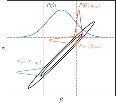
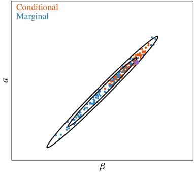
Figure 1: Illustration of conditional (pure Gibbs; orange) and marginal sampling (blue) algorithms for a highly correlated (Pearson’s correlation coefficient of $\rho=0.99$) two-dimensional Gaussian distribution (black contours). The initial position $(\beta_{\mathrm{init}},a_{\mathrm{init}})$ is indicated by a purple dot. Left: Comparison of un-normalized conditional $P(\beta\mid a_{\mathrm{init}})$ distribution evaluated at the initial position and the corresponding marginal $P(\beta)$ distribution; note that the latter is much wider than the former. Assuming $\beta$ samples drawn at the 10th percentile, the graphs along the vertical lines represent un-normalized conditial distributions $P(a\mid\beta)$ evaluated at the $\beta$ values drawn with the conditional (orange) and marginal (blue) distributions of $\beta$; note that the marginal sampling case results in a much longer step length between the initial and final sample values. Right: Samples of a standard Gibbs sampling chain (orange) using conditional sampling for both $a$ and $\beta$, and a sampling chain (blue) using marginal sampling for $\beta$ and conditional sampling for $a$. Both cases show the first 100 samples initialized from the purple point.

4.1 Joint amplitude and spectral parameter sampling

As summarized in Eqs. (5)–(11), the BeyondPlanck pipeline implements a Gibbs sampling chain iterating over all free parameters in the data model. While Gibbs sampling in general is a very powerful method for exploring complicated distributions, its main weakness is the inability to probe degenerate distributions. This problem is illustrated for a toy example in the left panel of Fig. 1: the black contours represents the 68 and 95 % confidence limits of a two-dimensional Gaussian distribution with a Pearson’s correlation coefficient of $\rho=0.99$. The purple point indicates the starting position of a Markov chain, while the dashed, grey horizontal line indicates the baseline of the corresponding conditional distribution $P(\beta\mid a_{\mathrm{init}})$, which itself is shown as an orange curve. Since the Gibbs sampling algorithm works by moving according to conditional distributions alone, the allowed step size in each iteration is very narrow compared to the full marginal distribution, shown as a blue distribution.

To illustrate the step size effect in the Gibbs sampler, we consider a Gibbs move in Fig. 1, starting with $\beta$ from the purple point. The relevant conditional distribution for $\beta$ is shown as an orange curve along the horizontal dashed gray line passing through the purple point and we can thus draw a random value from this distribution. This could for instance be the value indicated by the right-most vertical dashed gray line. According to the Gibbs sampling algorithm, we are required to draw a sample from the corresponding conditional distribution for $a$, which is indicated by the orange distribution aligned with the vertical dashed line. One possible outcome of this, after completing one full Gibbs iteration, is the orange point. Now, because each conditional distribution is much narrower than the corresponding marginal distributions, the relative Gibbs step size is very short, and it takes a very long time to move from one side of the joint distribution to the opposite. The result is poor Markov chain mixing and a very long correlation length. As a real-world illustration of this, the orange points in the right panel of Fig. 1 show the 100 first steps of an actual Gibbs chain with this precise target distribution. We see that less than half of the distribution is actually explored, and many thousands of samples will be required in order to probe the full distribution with this algorithm.

This problem is directly relevant for modern Bayesian intensity-based CMB component separation. For experiments such as Planck and WMAP, characterized by very high S/N, there are strong degeneracies between the foreground amplitudes, the foreground spectral parameters, and map-level monopoles. Explicitly, if one assumes that all spectral parameters and monopoles are known, then the conditional amplitude uncertainty is very small. Conversely, if we assume the amplitude and monopoles to be known, then the conditional spectral parameter uncertainties are small. However, when all parameters are unknown, the full uncertainties are significant.

For this reason, Gibbs sampling should usually be considered a last resort to handle an otherwise intractable distribution. If direct joint sampling methods are available, then those are usually more efficient. Fortunately, the Gibbs sampling method can be interleaved by any combination of conditional and joint steps while still maintaining the requirement of detailed balance (Geman & Geman 1984); also, the more steps that can be handled jointly, the more efficient the overall Gibbs chain will be. For the purposes of intensity-based CMB component separation, we therefore introduce a new special-purpose joint amplitude–spectral parameter step by exploiting the definition of a conditional distribution as follows,

$$P(\@vec{a},\beta\mid\@vec{m}_{\nu})=P(\beta\mid\@vec{m}_{\nu})\thinspace P(\@vec{a}\mid\@vec{m}_{\nu},\beta).$$ (19)

The first distribution on the right hand side is the marginal distribution of $\beta$ with respect to the data $\@vec{m}_{\nu}$, and the second distribution is the conditional distribution of $\@vec{a}$ with respect to $\beta$. This equation therefore implies that we may generate a joint sample by first drawing $\beta$ from its ”marginal” distribution, and then sample $\@vec{a}$ from the corresponding ”conditional” distribution:

$$\beta\leftarrow P(\beta\mid\@vec{m}_{\nu}),$$

$$\@vec{a}\leftarrow P(\@vec{a}\mid\@vec{m}_{\nu},\beta).$$

We note the absence of $\@vec{a}$ in the first distribution. We then need to derive sampling procedures for each of these two distributions. According to Bayes’ theorem:

$$P(\@vec{a},\beta\mid\@vec{m}_{\nu})=\frac{P(\@vec{m}_{\nu}\mid\@vec{a},\beta)P(\@vec{a},\beta)}{P(\@vec{m}_{\nu})},$$ (20)

where $P(\@vec{m}_{\nu})$ is just a normalization factor (often called the “evidence”), $P(\@vec{a},\beta)$ denotes optional priors, and the final factor is the likelihood function, $P(\@vec{m}_{\nu}\mid\@vec{a},\beta)\equiv\mathcal{L}(\@vec{a},\beta)$. From the compact data model in Eq. (3), we note that

$$\@vec{m}_{\nu}-\@tens{A}_{\nu}(\beta)\@vec{a}=\@vec{n}^{\mathrm{w}}_{\nu},$$ (21)

and since $\@vec{n}^{\mathrm{w}}_{\nu}$ is assumed to be zero-mean and Gaussian distributed with known variance, we can immediately use the following expression for the likelihood function:

$$\ln\mathcal{L}(\@vec{a},\beta)\propto-\frac{1}{2}\sum_{\nu}(\@vec{m}_{\nu}-\@tens{A}_{\nu}(\beta)\@vec{a})^{T}\thinspace\@tens{N}^{-1}_{\nu}\thinspace(\@vec{m}_{\nu}-\@tens{A}_{\nu}(\beta)\@vec{a}),$$ (22)

where $\@tens{N}_{\nu}$ is the noise covariance matrix of band $\nu$, which is diagonal in the case of pure white noise. The priors are less well-defined, and are left to the user to determine. In the following, we adopt Gaussian priors for spectral parameters and for notational convenience, we assume no spatial amplitude priors, $\@tens{S}^{-1}=\@tens{0}$.

We first consider the marginal spectral parameter distribution, $P(\beta\mid\@vec{m}_{\nu})$. This is derived by integrating Eq. (22) with respect to $\@vec{a}$, and this was done by Stompor et al. (2009) and Stivoli et al. (2010) as part of developing the Miramare component separation code. The result is expressed as:

$$\mathrm{ln}\thinspace\mathcal{L}_{\mathrm{marg}}(\beta) =\mathrm{ln}\int d\@vec{a}\;\mathrm{exp}\left[-\frac{1}{2}(\@vec{m}-\@tens{A}\@vec{a})^{T}\thinspace\@tens{N}^{-1}\thinspace(\@vec{m}-\@tens{A}\@vec{a})\right]$$

$$=\mathrm{const}-\frac{1}{2}(\@tens{A}^{T}\thinspace\@tens{N}^{-1}\thinspace\@vec{m})^{T}\thinspace(\@tens{A}^{T}\thinspace\@tens{N}^{-1}\thinspace\@tens{A})^{-1}\thinspace(\@tens{A}^{T}\thinspace\@tens{N}^{-1}\thinspace\@vec{m})$$

$$\quad\quad+\frac{1}{2}\mathrm{ln}\left|(\@tens{A}^{T}\thinspace\@tens{N}^{-1}\thinspace\@tens{A})^{-1}\right|,$$ (23)

where all terms should be interpreted as sums over frequencies. The same authors also introduced a so-called “ridge likelihood,” in which one does not marginalize over $\@vec{a}$, but rather sets $\@vec{a}$ equal to its maximum likelihood value for a given value of $\beta$. This may also be analytically evaluated, and is in fact identical to the above expression, with the exception of the last determinant term being excluded. We implemented support for both options in our codes. We note that this expression requires all data to be defined at the same angular resolution and so, all data must be smoothed to a common resolution before evaluating Eq. (23).

The second required distribution is $P(\@vec{a}\mid\@vec{m}_{\nu},\beta)$. This is a simple multi-variate Gaussian distribution in $\@vec{a}$, for which there are efficient samplers readily available (see, e.g., Appendix A of BeyondPlanck 2022 for details). One particularly efficient sampling equation is as follows:

$$\biggl{(}\sum_{\nu}\@tens{A}_{\nu}^{t}\@tens{N}_{\nu}^{-1}\@tens{A}_{\nu}\biggr{)}\@vec{a}=\sum_{\nu}\@tens{A}_{\nu}^{t}\@tens{N}_{\nu}^{-1}\@vec{m}_{\nu}+\sum_{\nu}\@tens{A}_{\nu}^{t}\@tens{N}_{\nu}^{-1/2}\eta,$$ (24)

where $\eta$ is a vector of random Gaussian $N(0,1)$ variates. This equation may be solved efficiently using preconditioned Conjugate Gradient methods (Shewchuk 1994), as discussed by Seljebotn et al. (2019).

These equations are integrated into the main BeyondPlanck Gibbs sampling loop according to the following steps. First, we run a short (typically a few hundred steps) standard Metropolis sampler (see Appendix A of BeyondPlanck 2022) for each spectral parameter, using the product of Eq. (23) and any desired priors to define the accept rate, that is, the relative number of Metropolis proposals being accepted (which should preferably stay between 0.3 and 0.7 for an efficient sampler). All data are smoothed to a common angular and pixel resolution before evaluating the expression. Immediately following the last Metropolis step, we draw one sample from $P(\@vec{a}\mid\@vec{m}_{\nu},\beta)$ using Eq. (24); it is critically important that no other parameters are updated between $\beta$ and $\@vec{a}$, as the previous value of $\@vec{a}$ is completely inconsistent with the new $\beta$ value, which is drawn marginally with respect to $\@vec{a}$.

Returning to Fig. 1, the improvement achieved by this joint two-step sampler is illustrated as blue distributions and points. Starting with the left panel, the fundamental difference between the joint and Gibbs samplers is that the first step in the $\beta$-direction is drawn from the full marginal distribution (horizontal blue distribution) instead of the conditional distribution (horizontal orange distribution). This is much wider, and covers by construction the full width of the underlying target distribution. One single proposal may therefore move from one side of the distribution to the other, and there is no memory of the previous parameter state. However, to obtain a valid sample, it is critically important to draw a corresponding sample from the appropriate conditional amplitude distribution (vertical blue distribution) immediately after the marginal move. Correspondingly, the blue points in the right panel shows 100 samples drawn with the joint sampler. In this case, they cover the full distribution very efficiently.

Figure 2 shows a similar comparison for AME $\nu_{\mathrm{p}}$ for a test chain that only explores the AME parameters in the BeyondPlanck data model with both methods. Also in this case, we see that the marginal sampler explores the full range much more efficiently than the conditional sampler.

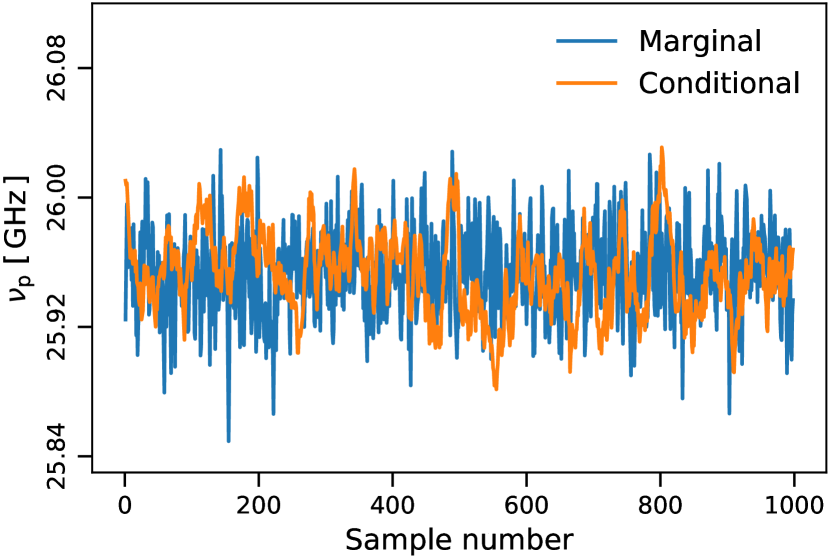
Figure 2: Comparison of AME $\nu_{\mathrm{p}}$ chains derived using the conditional (orange; Eq. 22) and marginal (blue; Eq. 23) samplers discussed in the text. For the purposes of this illustration, all other parameters than $\@vec{a}_{\mathrm{AME}}$ and $\nu_{\mathrm{p}}$ are fixed.

4.2 Component-based monopole determination

Next, we considered the problem of monopole determination for CMB experiments, which has long been one of the main challenges for parametric component separation methods (see, e.g., Planck Collaboration X 2016; Wehus et al. 2017, and references therein). The problem stems from the following challenge: For traditional CMB experiments and maximum likelihood mapmaking methods, there are no data-driven constraints on the monopoles in the derived frequency sky maps. For example, WMAP is explicitly differential in nature, measuring only differences between pairs of points, and therefore cannot by construction constrain the zero-level. For Planck, the high level of $1/f$ noise prohibits any useful constraints on the zero-levels. An important exception to this is COBE/FIRAS (Mather et al. 1994), which is absolutely calibrated; but its mK-level uncertainties are still orders of magnitude too large to be useful for modern CMB component separation purposes.

For this reason, several indirect methods have been established to determine the frequency map monopoles based on the morphology of the maps themselves. Four examples are mean subtraction in a small region (Planck Collaboration V 2014); fitting a plane-parallel co-secant model (Bennett et al. 2003; Planck Collaboration II 2016); imposing foreground SED consistency between neighboring frequencies (Wehus et al. 2017); and cross-correlation with external data sets with known zero-levels (Planck Collaboration VIII 2016). However, all of these methods have in common the fact that they operate on the basis of frequency maps and are aimed to determine the zero-level at a given frequency channel, before feeding these into traditional component separation algorithms. In this study, we have made the observation that it is, in fact, much simpler to determine the monopoles of the component amplitude maps and to then use these to deterministically set the frequency map monopoles through the resulting sky model. The frequency map zero-levels have thus no independent impact on any higher order analyses (most notably, the spectral parameters), but simply adjust to whatever the model dictates at any given moment.

As a result, the question that immediately rises considers how we may, in fact, determine the component monopoles. This must be done on a case-by-case basis, applying the most natural prior for each component. We note that any true monopole signal in the components that do not agree with the chosen priors will end up in the frequency map monopoles. Starting with the CMB case, this can either be set to zero or $2.7255\pm 0.0006\thinspace\mathrm{K}$ (Fixsen 2009), depending on whether we want sky maps without or with the CMB monopole. In practice, we additionally account for sub-optimal foreground modeling by applying a mask. For the current analysis, we derived the CMB monopole mask from a set of smoothed component amplitude maps, namely, by thresholding the sum of synchrotron, AME, free-free and thermal dust emission, all smoothed to 10^∘ FWHM. In addition, we masked out radio sources and any pixel with a reduced normalized $\chi^{2}$ higher than $5\thinspace\sigma$. The resulting mask is shown in Fig. 3, and has an accepted sky fraction of $f_{\mathrm{sky}}=0.64$. The monopole of the CMB component map is set to zero (or $2.7255\thinspace\mathrm{K}$) outside this mask, while simultaneously fitting for (but not modifying) the dipole component.

Regarding the free-free component, Planck Collaboration X (2016) found that the measured emission is strongly noise-dominated over large areas of the sky, with no detectable amplitude. Also, in this case, we therefore set the monopole to have zero mean outside a conservative mask. In this case, the mask is derived from the free-free amplitude map itself, evaluated at 30 GHz and smoothed to 10^∘ FWHM, and truncated at 5 $\mu$K_RJ. In addition, we excluded areas where the other foreground signals are high to account for signal-leakage into the free-free component, similarly to the CMB mask, but while thresholding the sum of all other components evaluated at 44 GHz. The resulting mask is shown in the bottom panel of Fig. 3, accepting $f_{\mathrm{sky}}=0.50$. We do note that any true unmasked free-free signal is by definition positive and this can bias the monopole also in the noise-dominated regime. Future works should aim to correct for this bias by directly estimating the residual free-free monopole in the unmasked region. We do note, however, that this bias will decrease as more high sensitivity data become available, as more and more of the free-free signal may be masked directly.

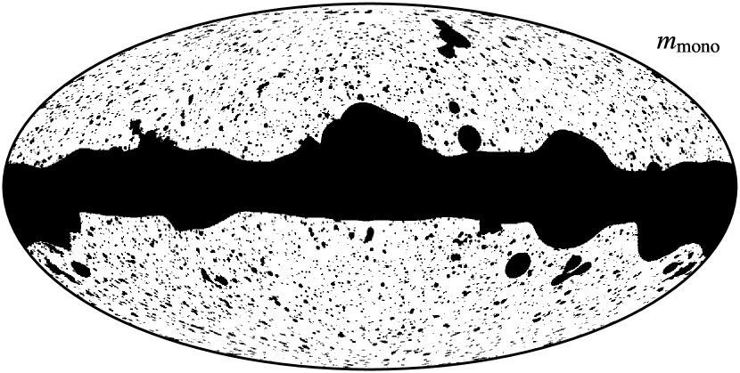
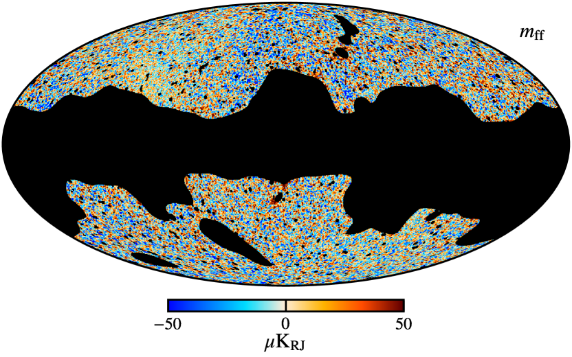
Figure 3: Masks used for signal amplitude zero-level and band monopole sampling: Frequency-band monopole and CMB amplitude zero-level (top) and free-free amplitude zero-level (bottom), with a free-free amplitude sample at an angular resolution of 30^′ FWHM plotted underneath.

In contrast, synchrotron emission as observed by the Haslam 408 MHz map is highly diffuse on the sky and there are no regions on the sky that can be assumed to be approximately clean of synchrotron emission, namely, exhibiting no synchrotron signal. In this case, the best estimates of the synchrotron amplitude are those already estimated for the Haslam 408 MHz map itself. In this paper, we adopt the zero-level correction of $8.9\pm 1.3\thinspace\mathrm{K_{CMB}}$ derived by Wehus et al. (2017). We marginalized over the uncertainty by drawing a random offset correction in every Gibbs iteration, as defined by a Gaussian distribution with the quoted mean and standard deviation.

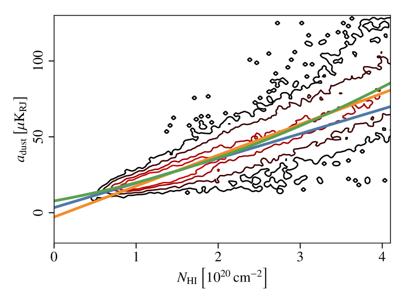
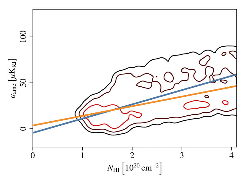
Figure 4: Cross-correlations between the H i column density $N_{\mathrm{H\thinspace\textsc{i}}}$ and (top) the thermal dust amplitude and (bottom) the AME amplitude. The thermal dust cross-correlation is evaluated at HEALPix resolution $N_{\mathrm{side}}=64$ and a common angular resolution of 60^′ FWHM, while the AME cross-correlation is evaluated at HEALPix resolution $N_{\mathrm{side}}=16$ and a common angular resolution of 10^∘ FWHM. The lines represent best-fit lines for pixels with H i column densities less than $2\cdot 10^{20}\thinspace\mathrm{cm}^{-2}$ (blue) or $4\cdot 10^{20}\thinspace\mathrm{cm}^{-2}$ (orange). The green curve is the best-fit second degree polynomial to pixels with H i column densities less than $4\cdot 10^{20}\thinspace\mathrm{cm}^{-2}$. The contour lines are plotted at 0.001, 0.01, 0.05, and 0.1 $N_{\mathrm{pix}}/(\thinspace\mu\mathrm{K_{RJ}}\;10^{20}\thinspace\mathrm{cm}^{-2}\;N_{\mathrm{side}}^{2}\thinspace)$; where only the lower three contour line values are plotted for AME. The contours have been smoothed for visualization.

For the thermal dust emission, we adopted essentially the same approach as the Planck HFI DPC (e.g., see Planck Collaboration III 2020), setting the zero-level through cross-correlation with H i column density observations (e.g., see Lenz et al. 2017), although with a few minor variations. First, we applied this method to the thermal dust component map, as opposed to individual frequency maps. Second, for Planck DR4 (Planck Collaboration LVII 2020), the HFI 545 GHz zero-level was set through a linear fit for pixels with $N_{\mathrm{H\thinspace\textsc{i}}}<4\cdot 10^{20}\thinspace\mathrm{cm}^{-2}$. However, as the 545–$N_{\mathrm{H\thinspace\textsc{i}}}$ scatter plot appeared to be non-linear around values of $N_{\mathrm{H\thinspace\textsc{i}}}=1.5\cdot 10^{20}\thinspace\mathrm{cm}^{-2}$, they also performed a second degree fit. We show in Fig. 4 a similar scatter plot between $N_{\mathrm{H\thinspace\textsc{i}}}$ and the thermal dust amplitude from one of our Gibbs samples, where we performed both a first and second degree polynomial fit to the plot at $N_{\mathrm{H\thinspace\textsc{i}}}<4\cdot 10^{20}\thinspace\mathrm{cm}^{-2}$. Furthermore, we also performed a linear fit at $N_{\mathrm{H\thinspace\textsc{i}}}<2\cdot 10^{20}\thinspace\mathrm{cm}^{-2}$ and we see that the intersection of the linear fit with a lower threshold is close to the intersection of the second degree fit. This raises the question of the uncertainty of the threshold value for the linear fit, as Planck Collaboration XXIV (2011) found a good correlation up to at least $N_{\mathrm{H\thinspace\textsc{i}}}=2\cdot 10^{20}\thinspace\mathrm{cm}^{-2}$. We therefore implement this cross-correlation method as a prior on the thermal dust zero-level using a range of thresholds, and for each Gibbs iteration we perform linear fits of $N_{\mathrm{H\thinspace\textsc{i}}}$ and the thermal dust amplitude with $N_{\mathrm{H\thinspace\textsc{i}}}$ threshold values ranging from 1.5 to 4 $[10^{20}\thinspace\mathrm{cm}^{-2}]$ with increments of 0.5. Then we draw the intersection value from a Gaussian distribution given the mean and variance of the linear fits, which is subtracted from the dust amplitude. This way, the uncertainty of the thermal dust amplitude zero-level also propagates through the pipeline.

The zero-level of the AME component is determined using the same procedure, noting that Planck Collaboration X (2016) demonstrated a very tight spatial correlation between AME and thermal dust emission on large angular scales. The only difference with respect to the thermal dust procedure is that we smooth all maps to a common angular resolution of 10^∘ FWHM and a HEALPix resolution of $N_{\mathrm{side}}=16$, and adopt thresholds of 2 to 4 $[10^{20}\thinspace\mathrm{cm}^{-2}]$, with increments of 0.5; both the smoothing and the lower resolution are imposed to reduce the impact of instrumental noise. A scatter plot between AME and $N_{\mathrm{H\thinspace\textsc{i}}}$ is shown in Fig. 4 for one arbitrary Gibbs sample.

With the introduction of component-based monopole priors, all frequency-band monopoles become free parameters and can be deterministically fitted. Explicitly, for each frequency channel we first subtract the predicted sky model as defined by Eq. (2) and then fit and subtract the residual monopole outside some mask. The mask should be defined such that it excludes areas on the sky prone to foreground mismodeling, hence we adopt the same mask as we do for the CMB monopole prior, shown in the top panel of Fig. 3. We note that this monopole adjustment needs to be done immediately after any change in any of the component maps, in order to not break the Gibbs chain, fully analogously to the immediate amplitude update that must follow any marginal spectral parameter move discussed in the previous section.

4.3 Joint spectral parameter and frequency-band monopole sampling

Returning to the AME–H i cross-correlation plot in Fig. 4, we notice that the zero-level is associated with a large statistical uncertainty. When sampling the AME peak frequency, $\nu_{\mathrm{p}}$, this uncertain monopole is also directly affected by the resulting SED changes, and corresponding monopole offsets are induced at all frequencies. If $\nu_{\mathrm{p}}$ is sampled conditionally with respect to the band monopoles, these will therefore tend to pull $\nu_{\mathrm{p}}$ towards the old value and thereby increasing the overall Markov chain correlation length.

This inefficiency may be alleviated by exploiting the new component-based monopole sampler described in Sect. 4.2. Since all frequency-band monopoles are now deterministically defined by the sky model, these can be adjusted jointly whenever that is modified. We therefore implement internal estimation of frequency band monopoles during the spectral parameter sampling algorithm, such that for each proposed spectral parameter value, we estimate a new band monopole value conditioned on the input amplitude and the proposed parameter value. The frequency band monopoles are updated together with the final parameter at the end of the sampling.

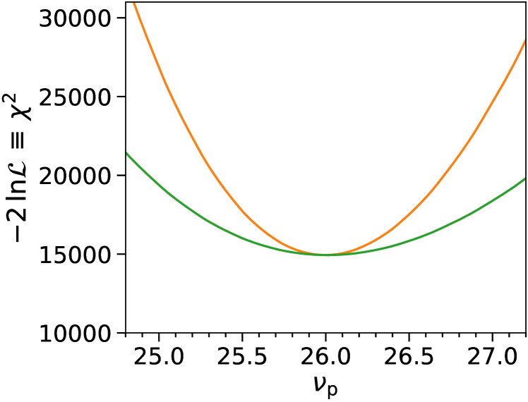
Figure 5: Comparison of AME $\nu_{\mathrm{p}}$ $\chi^{2}$ distributions with (green) and without (orange) monopole marginalization. These distributions are evaluated using the marginal spectral parameter likelihood given in Eq. (23), but the same qualitative behaviour holds irrespective of which spectral parameter distribution is used (conditional, ridge, or marginal): the distribution becomes significantly wider when marginalizing over band monopoles.

To illustrate the usefulness of this combined sampling step, we generate an idealized simulation that includes only AME signal and noise at each frequency channel, with an angular resolution of 10^∘ FWHM and a HEALPix resolution of $N_{\mathrm{side}}=16$. We choose an input peak frequency of $\nu_{\mathrm{p}}=26$ GHz, and adopt a zero-level from H i column density cross-correlation to 2 $\mu$K_RJ. Figure 5 shows the resulting log-likelihood (or $\chi^{2}$) distributions as evaluated from the marginal definition in Eq. (23), for cases both with (green curve) and without (orange curve) marginalizing over the frequency band monopoles. We see that by marginalizing over the band monopoles the log-likelihood function widens by a factor of 1.5–2. This translates into correspondingly longer Metropolis step sizes in the spectral index sampling steps, and thereby faster exploration of the full posterior distribution. The higher conditional S/N a given component has, the more important this effect will be.

4.4 Breaking small-scale degeneracies through spatial priors

The final algorithmic improvement presented in this paper is the introduction of informative spatial priors for foreground components, either in the form of purely algorithmic smoothing power spectrum priors or as actual informative Gaussian priors with a non-zero mean. The first of these has already been used in the latest Planck analyses (Planck Collaboration IV 2018; Planck Collaboration LVII 2020), but in the following, we generalize the approach to non-zero cases and we systematically show how different choices affect the final results.

Mathematically speaking, the only difference between an informative prior and a smoothing prior is whether a pre-existing mean map is assumed for the astrophysical component in question (in which case the prior is called “informative”) or whether the prior mean is assumed to be zero. Practically speaking, however, there is also an important difference between the prior variances in the two cases, since for informative priors the variance quantifies the allowed level of fluctuations around the mean map; while for smoothing priors, it quantifies the allowed level of fluctuations around zero. Thus, for informative priors a prior variance of zero is fully acceptable, in which case the output component map will be identical to the prior mean; while for a smoothing prior the variance should be larger than the actual component fluctuations in order to avoid oversmoothing.

We start by revisiting the sampling equation for the component amplitude maps, as defined by Eq. (24). This equation provides a sample from a posterior defined only by the likelihood itself. If we additionally want to impose a Gaussian prior on the amplitudes, as defined by a multi-variate Gaussian distribution, $N(\mu,\@tens{S})$, then this is generalized to:

$$(\@tens{S}^{-1}+\@tens{A}^{t}\@tens{N}^{-1}\@tens{A})\@vec{a}=\@tens{A}^{t}\@tens{N}^{-1}\@vec{m}_{\nu}+\@tens{S}^{-1}\mu+\@tens{A}^{t}\@tens{N}^{-1/2}\@vec{\eta}_{1}+\@tens{S}^{-1/2}\@vec{\eta}_{2}.$$ (25)

We refer to Appendix A in BeyondPlanck (2022) for an explicit derivation. In this expression, $\mu$ has the same dimension as $\@vec{a}$, and represents the prior mean for $\@vec{a}$, while $\@tens{S}$ is an associated prior covariance matrix that defines the “strength” of the prior, fully analogous to the usual standard deviation, $\sigma$, of a Gaussian uni-variate prior. Thus, if $\@tens{S}=\@tens{0}$, the final solution for $\@vec{a}$ will be identical to $\mu$, while if $\@tens{S}\rightarrow\infty$ (or, equivalently, $\@tens{S}^{-1}=\@tens{0}$), then the prior term vanishes, and one is left with the original likelihood expression in Eq. (24). For reference, we note that the previous Planck analyses (Planck Collaboration IV 2018; Planck Collaboration LVII 2020) set $\mu=0$ in this equation and only used $\@tens{S}$ to impose smoothness on $\@vec{a}$.

Computationally speaking, introducing informative priors with non-zero means in Eq. (25) represents no additional algorithmic complications compared to the prior-free case: the equation is in both cases solved using the same preconditioned conjugate gradient implementation. If anything, the equations are actually a bit easier to solve with informative priors, as they reduce degeneracies between different parameters, and thereby reduce the condition number of the coefficient matrix on the left-hand side of the equation. As pointed out by Seljebotn et al. (2019), from an algorithmic point of view an informative prior defined in terms of a mean map with a specified covariance may simply be considered to be a new independent data set with sensitivity only to the component in question and it therefore provides orthogonal information with respect to the likelihood term contributions. Rather, the main challenge regarding priors is how to define them in a useful and controlled manner that does not significantly bias or contaminate the final posterior distribution and this must be assessed on a case-by-case basis.

In the current BeyondPlanck analysis, we followed Planck Collaboration IV (2018) and define $\@tens{S}$ in harmonic space, giving different prior weights to different angular scales. Explicitly, each component map is defined in terms spherical harmonics:

$$\@vec{a}=\sum_{\ell,m}a_{\ell m}Y_{\ell m},$$ (26)

and we define the prior covariance matrix as:

$$\@tens{S}=\@tens{S}_{\ell m,\ell^{\prime}m^{\prime}}\equiv\left<a_{\ell m}a^{*}_{\ell^{\prime}m^{\prime}}\right>=P_{\ell}\delta_{\ell\ell^{\prime}}\delta_{mm^{\prime}},$$ (27)

where $P_{\ell}$ is an angular prior power spectrum for $\@vec{a}$, which, again, is fully analogous to the standard deviation of a Gaussian prior, but now defined per angular multipole.

4.4.1 Algorithmic smoothing priors

Starting with the algorithmic smoothing priors adopted by Planck 2018, we note that if we define $P_{\ell}^{\@vec{a}}$ to be an estimate of the true angular power spectrum of $\@vec{a}$, then the following power spectrum prior,

$$P_{\ell}=P^{\@vec{a}}_{\ell}e^{-\ell(\ell+1)\sigma^{2}},$$ (28)

simply represents a Gaussian smoothing prior of $\@vec{a}$ with a smoothing kernel width equal to $\sigma$, which often is defined in terms of $\theta_{\mathrm{FWHM}}=\sqrt{8\ln 2}\sigma$. We call this an algorithmic smoothing prior, as it explicitly pushes the solution to be smooth on small angular scales. We also note that $P_{\ell}^{\@vec{a}}$ does not have to be an accurate estimate of the true component power spectrum, but it should in general be greater than the true spectrum, in order to prevent the prior from being overly constraining. This is again fully analogous to choosing a prior width that is wider than the expected target distribution in standard univariate analysis problems. Thus, simply setting $P_{\ell}^{\@vec{a}}$ to a constant that is a few times larger than the expected spectrum is usually a perfectly good choice.

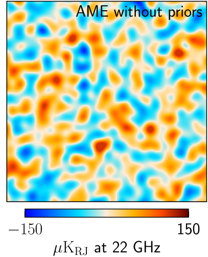
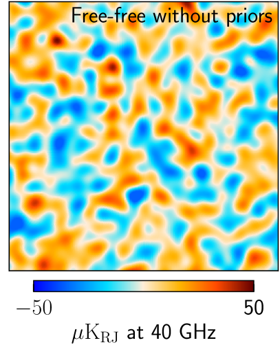
Figure 6: Comparison of AME (left) and free-free (right) amplitude maps derived without any spatial priors in a $20\times 20^{\circ}$ field centered on the Galactic South Pole, $(l,b)=(0^{\circ},-90^{\circ})$ at an angular resolution of 60^′ FWHM. We note the striking anti-correlation between the two maps.

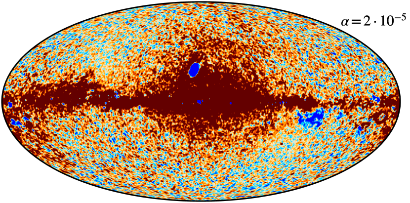
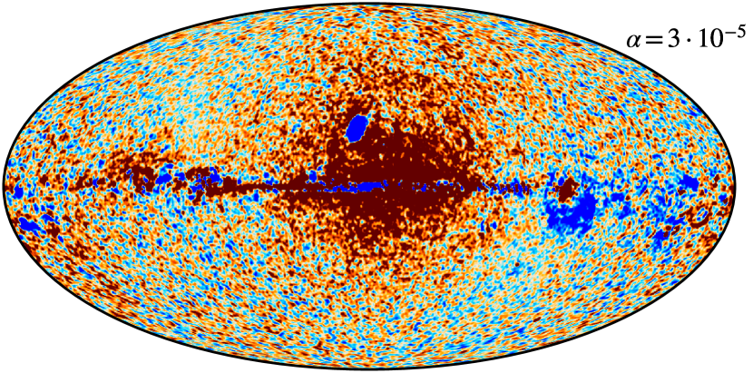
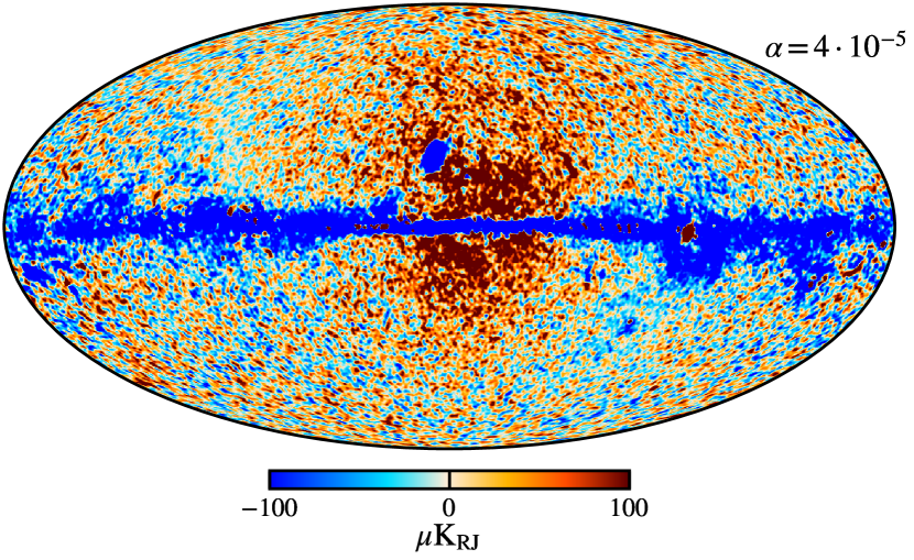
Figure 7: Difference maps between the derived amplitude and prior maps for AME for three different 857 GHz scaling factors. From top to bottom, the three panels show scaling factors of $\alpha=2\cdot 10^{-5}$, $\alpha=3\cdot 10^{-5}$, and $\alpha=4\cdot 10^{-5}$.

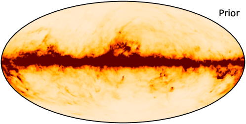
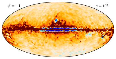
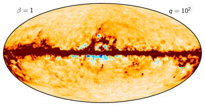
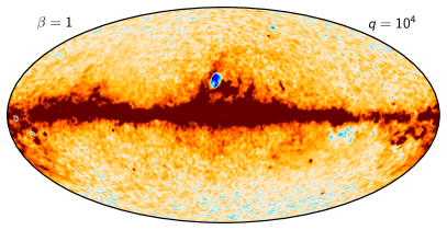
Figure 8: Effects of the spatial prior on the sampled AME amplitude. AME amplitude prior map, derived by scaling the Planck DR4 857 GHz by $\alpha=3\cdot 10^{-5}$ and smoothing to $10{{}^{\scriptstyle\prime}}$ FWHM (top). Derived AME amplitude maps for four different spatial prior combinations (bottom), $\hat{D}_{\mathrm{AME}}(\ell)=q\thinspace(\ell/\ell_{0})^{\beta}$. Rows show results for $q=10^{2}\thinspace\mu\mathrm{K}_{\mathrm{RJ}}^{2}$ and $10^{4}\thinspace\mu\mathrm{K}_{\mathrm{RJ}}^{2}$, respectively, while columns show results for $\beta=-1$ and 1.

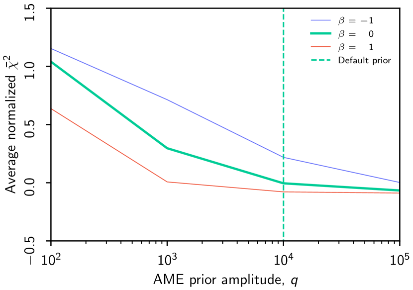
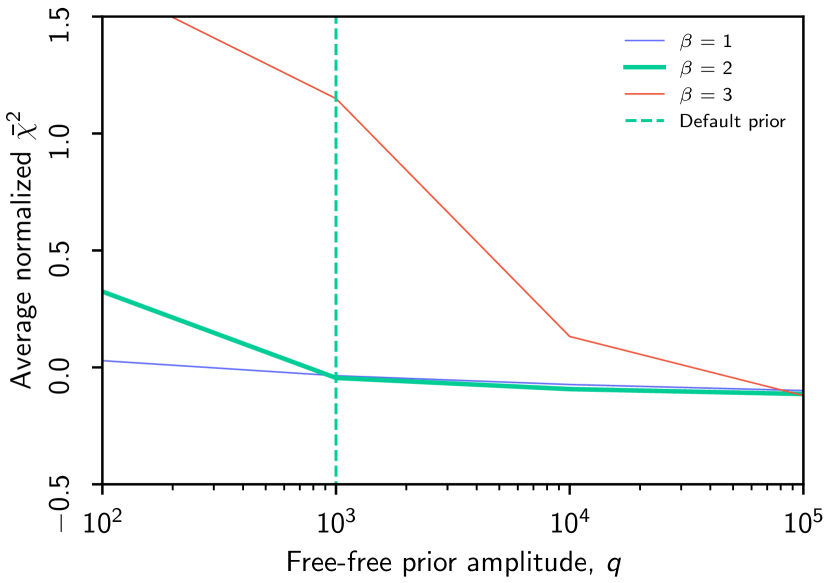
Figure 9: Average $\bar{\chi}^{2}$ per $N_{\mathrm{side}}=16$ pixel as a function of AME (top) and free-free (bottom panel) prior amplitude, $q$, where $\bar{\chi}^{2}\equiv(\chi^{2}-n_{\mathrm{dof}})/\sqrt{2n_{\mathrm{dof}}}$ and $n_{\mathrm{dof}}=15\thinspace 400$. Colored solid lines show results for different tilt parameters, $\beta$, and the intersection between the thick green curve and dashed line indicates the prior combination adopted for the main BeyondPlanck analysis.

It is important to note that Eq. (28) is indeed just a prior, and not a deterministic postprocessing smoothing operator. This has both advantages and drawbacks that are important to be aware of when using the products from the analysis. The main advantage is that signal-dominated localized objects (for instance point sources) are not excessively smoothed when applying the smoothing as a prior. The main disadvantage is that the effective angular resolution of the amplitude map becomes spatially varying and depends on the local S/N in a given pixel; if the S/N is high, the angular resolution will be determined by the resolution of the data, while if the S/N is low, it is given by $\theta_{\mathrm{FWHM}}$. This is similar to the GNILC method (Remazeilles et al. 2011), which also implements S/N dependent angular resolution. The main difference between the two methods is that while GNILC requires regions of different resolutions to be pre-defined, the current approach automatically and dynamically adopts the resolution while solving Eq. (25).

In the current BeyondPlanck analysis, where the main scientific target is CMB power spectrum and cosmological parameter estimation, we do not impose any priors on the CMB component amplitudes, but we do impose a Gaussian smoothing prior for thermal dust emission in intensity with $\theta=5{{}^{\scriptstyle\prime}}$ FWHM and $P_{\ell}^{\@vec{a}}=10^{7}\thinspace\mu\mathrm{K}_{\mathrm{RJ}}^{2}$ at 545 GHz. For studies that are primarily interested in the angular power spectrum of thermal dust emission, it would be more useful to instead impose a Lambda-Cold-Dark-Matter ($\Lambda$CDM) spectrum on the CMB amplitude map, and no priors on the thermal dust spectrum. Then the resulting thermal dust power spectrum would be an unbiased estimator; with the current analysis, the thermal dust spectrum will be biased low on small angular scales due to the smoothing prior. We also impose a Gaussian smoothing prior on synchrotron emission in intensity, with $\theta=60{{}^{\scriptstyle\prime}}$ FWHM and $P_{\ell}^{\@vec{a}}=3\cdot 10^{14}\thinspace\mu\mathrm{K}_{\mathrm{RJ}}^{2}$ at 408 MHz.

4.4.2 Informative Gaussian spatial priors

For AME and free-free emission, we adopt informative priors with $\mu\neq 0$. The reason for this is simply that the limited data combination considered in the current BeyondPlanck analysis (see Table 1) is inadequate for constraining all of AME, free-free, and CMB separately without additional information; when future observations from, for instance, C-BASS (King et al. 2010) and QUIJOTE (Génova-Santos et al. 2015) become publicly available and integrated in the analysis, this will hopefully no longer be necessary. As an illustration of the problem, Fig. 6 compares the AME and free-free amplitude maps derived without any priors near the Galactic South Pole; even at a visual level, these two maps are nearly perfectly anti-correlated, with no true constraining power on their own. This also makes other components (most importantly the CMB) susceptible to small systematic residual mismatches between the AME and free-free components and it significantly increases the CMB noise.

Starting with the AME case, we first note that the prior-free Planck 2015 analysis (Planck Collaboration X 2016) found a very strong spatial correlation between their AME and thermal dust component maps at an angular resolution of $1^{\circ}$ FWHM. In general, a high degree of correlation between these components is expected from current theoretical AME models (e.g., Erickson 1957; Draine & Lazarian 1998; Ali-Haïmoud 2010; Silsbee et al. 2011; Hensley & Draine 2020), although the specific correlation coefficient depends on model details. Based on these observations, we adopted the Planck DR4 857 GHz map (Planck Collaboration LVII 2020) as a spatial mean template for AME, that is, $\mu$ in Eq. (25). However, before it can be inserted into Eq. (28), it must be adjusted in amplitude to account for the mean SED difference between thermal dust emission at 857 GHz and AME at 22 GHz. To do this, we solved Eq. (28) using the 857 GHz map scaled by a range of values between $\alpha=2\cdot 10^{-5}$ and $4\cdot 10^{-5}$ as the AME prior. We then took the difference between the derived amplitude map and the input prior and adopted the scaling factor for which the difference is smallest as our default prior. Example difference maps are shown in Fig. 7 and we adopted $\alpha=3\cdot 10^{-5}$ as our default prior.

The final step is to define the strength of this prior, as given by $P_{\ell}$. Ideally, we want the prior to be stronger (i.e., $\@tens{S}$ to be smaller) for the noise-dominated small angular scales and looser for the signal-dominated large angular scales. To quantify these considerations, we must define the following a power-law prior power spectrum for AME:

$$P_{\ell}^{\mathrm{AME}}=q\left(\frac{\ell}{\ell_{0}}\right)^{\beta},$$ (29)

where $q$ is an overall amplitude at a pivot multipole, $\ell_{0}$, and $\beta$ is a tilt parameter. A negative (positive) $\beta$ results in a stronger (weaker) prior at high multipoles and a smaller (higher) amplitude, $q,$ gives a stronger (weaker) prior on all angular scales.

Figure 8 compares the resulting AME amplitude maps for various choices of $q$ and $\beta$ (bottom panels) with the prior mean map (top panel). Here we see that a high value of $q=10^{4}\thinspace\mu\mathrm{K}_{\mathrm{RJ}}^{2}$ leads to very similar solutions for $\beta=-1$ and $\beta=1$, indicating that the prior is largely irrelevant, and the solution is data dominated. We also note that there is substantial instrumental noise at high latitudes. For $q=10^{2}\thinspace\mu\mathrm{K}_{\mathrm{RJ}}^{2}$, the maps are notably smoother at high latitudes, but we also see clear smoothing artefacts near the Galactic plane, corresponding to harmonic space ringing from the Galactic plane. A value of $\beta=-1$ leads to sharper edges than $\beta=1$.

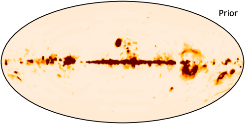
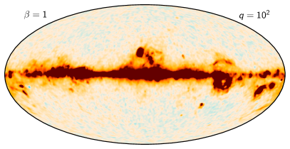
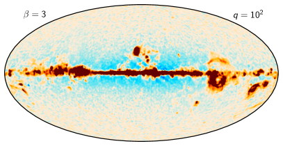
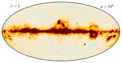
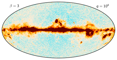
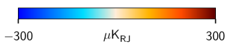
Figure 10: Free-free amplitude prior map, adopted from the Planck 2015 analysis which includes HFI observations (top). Derived free-free amplitude map for four different spatial prior combinations (bottom), $\hat{D}_{\mathrm{ff}}(\ell)=q\thinspace(\ell/\ell_{0})^{\beta}$. Rows show results for $q=10^{2}\thinspace\mu\mathrm{K}_{\mathrm{RJ}}^{2}$ and $10^{4}\thinspace\mu\mathrm{K}_{\mathrm{RJ}}^{2}$, respectively, while columns show results for $\beta=1$ and 3.

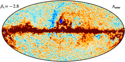
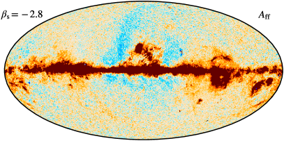
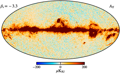
Figure 11: AME (left) and free-free (right) amplitude maps derived for two different synchrotron spectral indices. The top row shows results for $\beta_{\mathrm{s}}=-2.8$, while the bottom row shows results for $\beta_{\mathrm{s}}=-3.3$. In the top row, we see a negative synchrotron-like (see Fig. 20) imprint, which is not present in the bottom row.

To actually determine the parameters used for the final prior, we solve Eq. (28) over a grid in $q$ and $\beta$ and evaluate, as follows,

$$\chi^{2}(q,\beta)\equiv\sum_{\nu,p}\left(\frac{m_{\nu,p}-s_{\nu,p}(q,\beta)}{\sigma_{\nu,p}}\right)^{2}$$ (30)

for each configuration, where $s$ is the derived sky model in each case. The results from this evaluation are shown in the top panel of Fig. 9 in terms of the normalized reduced $\bar{\chi}^{2}\equiv(\chi^{2}-n_{\mathrm{dof}})/(2n_{\mathrm{dof}})$ where $n_{\mathrm{dof}}$ is the number of degrees of freedom; for a perfect model fit and $n_{\mathrm{dof}}\gg 1$, this quantity should be distributed approximately as a Gaussian distribution with zero mean and unit standard deviation. For $q=10^{2}\thinspace\mu\mathrm{K}_{\mathrm{RJ}}^{2}$ and $\beta=0$, we see that $\bar{\chi}^{2}\approx 1$, which indicates a clear excess residual. However, for $q=10^{4}\thinspace\mu\mathrm{K}_{\mathrm{RJ}}^{2}$ and $\beta=0$, this excess is greatly diminished, while there still is some effect from the prior. In the following, we adopt this latter combination as our default AME prior.

For free-free emission, there are no corresponding full-sky independent spatial templates available in the literature. Observations of H$\alpha$ (Finkbeiner 2003) or radio recombination lines (RRL; Alves et al. 2015) might serve useful roles, but both are associated with significant short-comings for the purposes of the current analysis: the H$\alpha$ observations lack most of the Galactic plane signal due to dust absorption, while the RRL observations only cover a part of the Galactic plane. For now, the best available full-sky free-free tracer is in fact the Planck 2015 free-free map (Planck Collaboration X 2016), which is based on the same data set as studied in the current paper, but additionally (and critically) the Planck HFI observations as well. We therefore adopted this map as a spatial prior in the current analysis, while recognizing that this is strictly speaking not admissible in the Bayesian framework; some data (i.e., LFI, WMAP, and Haslam) are used twice to constrain free-free emission and the resulting uncertainties will therefore be underestimated. In practice, this solution is a way of integrating HFI observations into the analysis without directly affecting the CMB component. A critical goal for near-future work is to integrate HFI observations directly into the analysis in the form of frequency maps and at that point, this informative free-free prior will be removed.

We adopted the same parametric function for free-free emission as for AME, defined by Eq. (29) and adjusted the free parameters in the same way. The results from this optimization are shown in the bottom panel of Fig. 9 and we adopted $q=10^{3}\thinspace\mu\mathrm{K}_{\mathrm{RJ}}^{2}$ and $\beta=2$ in this case. A comparison of different prior choices with the actual input prior map is shown in Fig. 10.

The only algorithmic difference with respect to AME is that we additionally imposed a Gaussian smoothing for free-free emission, as per Eq. (28) with $\theta=30{{}^{\scriptstyle\prime}}$ FWHM. This is done to account for the fact that the distribution of free-free emission is highly localized on the sky and therefore requires a high maximum multipole moment to capture all significant structures; the additional Gaussian smoothing ensures that no ringing emerges from the high-$\ell$ truncation.

5 Validation by simulations

In order to validate the component separation implementations, we ran Commander on the simulated data as described in Sect. 3.2. In this section, we describe the efficacy of the algorithmic developments by comparing the input foreground sky maps with the resulting mean of an ensemble of 300 component separation samples as produced by Commander. As described in Sec. 6.1, the only spectral parameter which is sampled and constrained by data is the AME peak frequency, $\nu_{\mathrm{p}}$, which is determined as a full sky value.

For the amplitude maps, we defined a new variable to represent the relative difference between the input amplitude map and the results of running the simulation through the Commander component separation procedure. We define $\epsilon$ as the relative difference given by:

$$\epsilon_{c}=\frac{\@vec{a}_{c}^{\mathrm{in}}-\@vec{a}_{c}^{\mathrm{out}}}{\@vec{a}_{c}^{\mathrm{in}}},$$ (31)

where, again, $c$ is an astrophysical sky component, $\@vec{a}^{\mathrm{in}}$ is the input simulation amplitude map, and $\@vec{a}^{\mathrm{out}}$ is the mean amplitude map of the component separation samples.

The results of the amplitude maps, represented in terms of the relative difference maps defined in Eq. 31, are summarized in Fig. 12. Inspecting the difference maps shows that there is good agreement with the input amplitude map, with departures from small relative differences in parts of the sky which are easy to explain. Notably, both the free-free and AME components show high levels of noisy departures off of the Galactic plane. Compared to the relative difference between two samples within component separation, the relative differences seen here are small. We see that in the high S/N observations along the Galactic plane, the agreement is excellent, with the outline of each components amplitudes clearly defined.

For the other three sky components, we see even better agreement. Unsurprisingly, the thermal dust amplitude map shows excellent agreement over the majority of the sky, though with deviations at the 10-20% level in the low signal-to-noise regions of the sky. Finally, the synchrotron amplitude map shows very small differences in $\epsilon_{\rm s}$, though the imprint of the component is significantly less notable here than in the other components.

The results of the 300 samples for the full sky spectral parameters and band monopoles can be seen in Figs. 13 and 14 respectively. Much like the sky component maps, we see excellent agreement with the input values for both spectral parameters and the band monopoles. We note that both the spectral indices and the band monopoles show a few samples which are significant deviations from the input value. This is to be expected, and is in fact an intention of the algorithms implemented in this work. As described in Sec. 4.3, the marginalization over the band monopoles allows for a broader log-likelihood, corresponding to a more complete exploration of the underlying distribution.

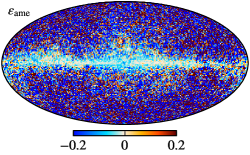
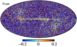
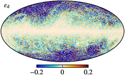
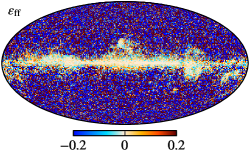
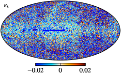
Figure 12: Relative difference maps, $\epsilon_{i}$, for each of the sky components within the simulated BeyondPlanck dataset. Top row: AME, CMB, and thermal dust maps. Bottom row: Free-free and synchrotron maps.

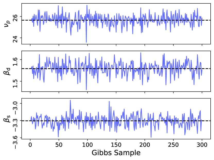
Figure 13: Full sky spectral parameters as a function of sample (blue) for the controlled simulation. The nominal input value of the simulation is overlayed as the black dashed line.

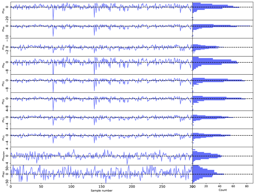
Figure 14: Band monopoles for each of the simulated frequency bands as a function of sample. The nominal input value is given by the overlaid black dashed line. The right panel shows the distribution of the samples.

6 BeyondPlanck analysis and posterior distributions

We now turn our attention to the actual BeyondPlanck analysis and intensity component posterior distributions derived from the data combination discussed in Sect. 3. The results described in this section represent the intensity foreground results of the BeyondPlanck project and are a practical demonstration of the algorithms described and tested in Sects. 4 and 5 respectively. We once again note that the goal of the BeyondPlanck project is not to derive a new state-of-the-art astrophysical component model within the relevant CMB frequency range (given that critical data sets such as Planck HFI and WMAP $K$-band are not included), but rather to lay the algorithmic groundwork for a statistically robust community-wide sky model, as will be implemented through the Open Science Cosmoglobe community effort. As far as Bayesian intensity sky modeling is concerned, Planck Collaboration X (2016) still represents a state of the art approach.

6.1 Spectral parameter prior tuning

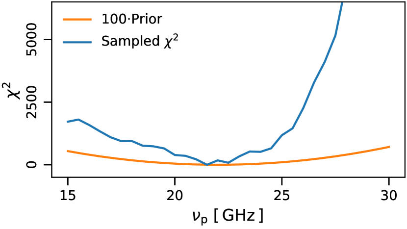
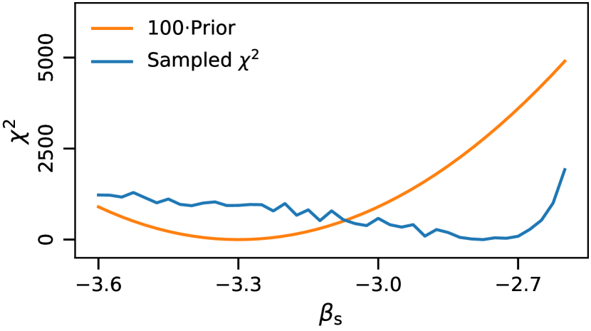
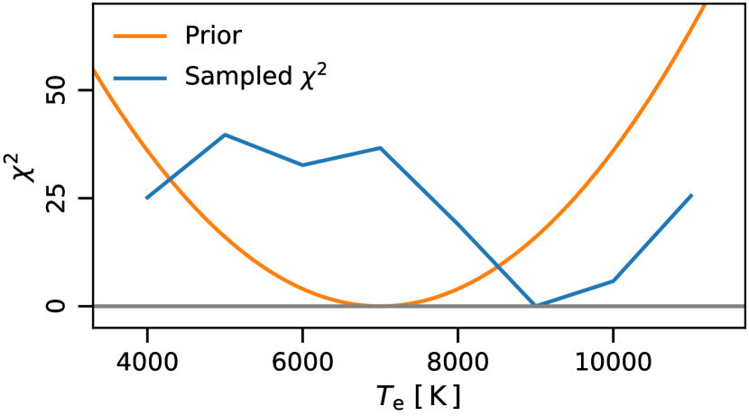
Figure 15: $\chi^{2}$ distributions (blue curves) from coarse grid evaluation of each free spectral parameters. From top to bottom, the panels show 1) AME peak frequency, $\nu_{\mathrm{p}}$; 2) synchrotron spectral index, $\beta_{\mathrm{s}}$; and 3) free-free electron temperature, $T_{\mathrm{e}}$. The minimum ${\chi}^{2}$ value for each parameter has been subtracted in each case. Orange curves show the priors adopted for the given component; see Table 2. The prior values for $\beta_{\mathrm{s}}$ and $\nu_{\mathrm{p}}$ have been scaled by a factor of 100 to fit in the plot with the derived ${\chi}^{2}$ values.

Before presenting the BeyondPlanck Markov chains and posterior distributions, there is still one task that must be completed before the algorithm described in Sect. 2 is carried out to completion, namely, finalizing the informative spectral parameter priors. With the reduced number of data sets included in this work, we have reduced constraining power when sampling spectral parameters, and strong priors are required for most spectral SED parameters. With this in mind, we can assume that all free parameters can only be fitted with a single constant value over the full sky, at least for now. Already at this stage, we fix the thermal dust temperature, $T_{\mathrm{d}}$, at the sky map derived by Planck DR4 (Planck Collaboration LVII 2020), noting that LFI has no constraining power for this particular parameter.

Even though LFI should have some constraining power of the thermal dust spectral index, $\beta_{\mathrm{d}}$, the thermal dust and AME components are found to be highly degenerate with the limited data set used in this work. A joint fit of the AME $\nu_{\mathrm{p}}$ and $\beta_{\mathrm{d}}$ would therefore lead to unphysical results, with preliminary analyses showing that the $\beta_{\mathrm{d}}$ diverged to values $\beta_{\mathrm{d}}>2,$ raising $\nu_{\mathrm{p}}$ to much higher frequencies. The uncertainty in the $\beta_{\mathrm{d}}$ value is important for error propagation and, thus, we must simply marginalize over the adopted prior, instead of trying to constrain $\beta_{\mathrm{d}}$ with the current data set.

For each free spectral parameter, we created a dedicated sampling mask, where we exclude regions on the sky where the other components are strong in order to reduce potential modeling mismatch errors to propagate between the various components. These masks are created from the amplitude maps of the modeled components, evaluated at 44 GHz and smoothed to 10^∘ FWHM. In addition, we masked radio sources by thresholding the Planck 30 GHz compact source map at three different angular resolutions, namely, at native resolution and at 1^∘ and 10^∘ FWHM. For $\beta_{\mathrm{s}}$ and $\nu_{\mathrm{p}}$, we excluded regions of the sky where any other component signals is greater than 40 $\mu$K_RJ; while for $T_{\mathrm{e}}$ , we excluded the areas where the other components are greater than 50 $\mu$K_RJ. For all parameters, we exclude any pixel for which the smoothed radio sources are stronger than 30 $\mu$K_RJ. Finally, we masked out regions of the sky contributing to the largest 15 % of a 10^∘ FWHM $\chi^{2}$ map to exclude regions with large known modeling errors. The accepted sky fractions of the resulting masks are $f_{\mathrm{synch}}=0.66$, $f_{\mathrm{ff}}=0.74$, and $f_{\mathrm{AME}}=0.66$, respectively.

For each free parameter, we adopted a Gaussian informative prior with some mean and standard deviation, $P(\beta)=N(\mu_{\mathrm{\beta}},\sigma_{\mathrm{\beta}}^{2})$. The prior parameters are informed by literature results and listed in Table 2. For synchrotron emission, we note that few intensity-based constraints are available for frequencies higher than 30 GHz in the literature and we therefore adopted $\beta_{\mathrm{s}}=-3.3\pm 0.1,$ as derived from polarization measurements in Planck Collaboration V (2020). We also note that we have attempted to use flatter mean values of $\beta_{\mathrm{s}}=-3.1$ and $-3.0$, as suggested from low-frequency surveys, but these result in obvious artefacts in the current analysis in the form of a significantly overestimated synchrotron amplitude at 30 GHz. As an example, Fig. 11 compares the AME and free-free amplitude maps derived for two different values of $\beta_{\mathrm{s}}$, namely, $\beta_{\mathrm{s}}=-2.8$ and $-3.3$. While neither of these solutions produce an excess $\chi^{2}$ and, therefore, a free likelihood-driven fit is unable to distinguish between them, it is obvious from visual inspection that the former spectral index leads to clear synchrotron leakage into both the AME and free-free components. With a prior of $\beta_{\mathrm{s}}=-3.3\pm 0.1$, the nonphysical flat-index solutions are largely excluded, while some parameter space is still allowed toward the steeper end to explore degeneracies. Another approach of reducing the predicted amplitude at CMB frequencies is by introducing a negative curvature in the synchrotron SED (as discussed in Sect. 2.2) and when comparing the results from this paper with previous results, it is important to ensure that the models are compatible.

Given the listed priors, we performed a coarse $\chi^{2}$ grid evaluation for each free parameter, conditioning on all other spectral parameter means, but allowing for amplitudes and band monopoles to adjust to the given spectral parameter. The resulting $\chi^{2}$’s (evaluated at a HEALPix resolution of $N_{\mathrm{side}}=16$) are shown in Fig. 15.

Starting with AME $\nu_{\mathrm{p}}$, shown in the top panel, we see that the $\chi^{2}$ is well-defined with a typical best-fit value around 22 GHz. The actual $\chi^{2}$ values show rapid increases at both lower and higher values with variations ranging in the thousands, and correspondingly, the prior (which is on the order of unity) is therefore largely irrelevant. It is clear that the current data combination has significant constraining power for $\nu_{\mathrm{p}}$.

The second panel shows similar results for $\beta_{\mathrm{s}}$. In this case, we see a rapid $\chi^{2}$ increase for $\beta\lesssim-2.7$, but it is otherwise slowly increasing for smaller values of $\beta_{\mathrm{s}}$ in the region $\beta_{\mathrm{s}}<-3.2$, becoming almost flat. Additionally, we already know from Fig. 11 that spectral indices flatter than $\beta_{\mathrm{s}}\lesssim-2.8$ lead to clearly contaminated AME component maps, even if the $\chi^{2}$ is not able to identify this. At the same time, the actual $\chi^{2}$ variations are indeed larger than the prior, and this typically indicates that the algorithm prefers to use this unconstrained degree of freedom to fit other degrees of freedom, for instance, modeling errors in the thermal dust model. To avoid pathological solutions, we instead chose to marginalize explicitly over the prior and disable the likelihood term entirely when sampling this parameter. In other words, we simply marginalized over the adopted prior, but we did not attempt to constrain $\beta_{\mathrm{s}}$ with the current data set.

The same considerations hold to an even greater extent for the last parameter. For the electron temperature, $T_{\mathrm{e}}$, the $\chi^{2}$ variations are entirely spurious and we therefore disable the likelihood term for $T_{e}$.

In summary, the only spectral parameter that the current data set is able to robustly constrain in intensity is the AME peak frequency, $\nu_{\mathrm{p}}$. All others are either drawn from their corresponding priors in the current analysis or frozen. We note that introducing additional data sets to constrain these parameters is a critically important next step for future works.

With $\beta_{\mathrm{s}}$ and $\beta_{\mathrm{d}}$ drawn from priors and $T_{\mathrm{e}}$ frozen, we find that the mask used in the coarse grid sampling of $\nu_{\mathrm{p}}$ is too conservative when sampling $\nu_{\mathrm{p}}$, masking out too much of the galactic plane and leading to large dust-like residual signals in the LFI 30 GHz and the WMAP $Ka$ channels. Additionally, a more dust-like signal was found to be leaking into the free-free component amplitude. In order to limit these effects, a less conservative mask had to be used. The mask used to sample $\nu_{\mathrm{p}}$ in the final BeyondPlanck production is generated by excluding all pixels with values above 200 $\mu$K_RJ of the free-free amplitude at both 30^′ and 2^∘ FWHM angular resolution evaluated at 40 GHz; all pixels with values above 100 $\mu$K_RJ of the point source amplitudes smoothed with a 1^∘ FWHM beam evaluated at the LFI 30 GHz band frequency; and the regions of the sky contributing to the largest 2.5 % of the $\chi^{2}$. The accepted sky fraction of the resulting mask is $f_{\mathrm{AME}}=0.91$.

6.2 Markov chain trace plots and correlations

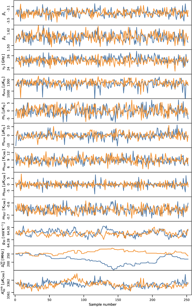
Figure 16: Trace plots of a set of sampled component separation parameters and selected instrument parameters, including absolute calibration ($g$), bandpass shift $(\Delta_{\mathrm{bp}})$, and the Solar CMB dipole ($A_{\mathrm{dp}}^{\mathrm{cmb}}$) from a naive mono- and dipole estimate using the band monopole mask, as described in Fig. 3. The parameter $a_{\mathrm{ame}}$ is the AME amplitude evaluated at 10^∘ FWHM and $N_{\mathrm{side}}=16$ of the pixel at Galactic coordinates $(l,b)=(31^{\circ},5^{\circ})$. Parameters from chain 1 are plotted in blue and chain 2 in orange.

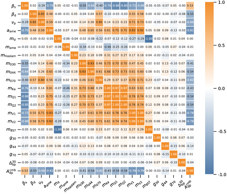
Figure 17: Correlation coefficient plot of local deviation, from a running mean of five prior and five succeeding samples of the sampled spectral parameters, component cross-correlation intersections, frequency band monopoles, absolute gain calibration, LFI 30 GHz bandpass shift, and CMB dipole amplitude, all as described in Fig. 16.

With the data, sampling algorithms, and priors in place, we are ready to consider the actual Markov chain results. As described by BeyondPlanck (2022), for the final analysis, we produced two independent chains, each with 750 samples.

Figure 16 shows the first 250 samples for a selection of relevant parameters. Several points are worth noting in this figure. First, we note that the burn-in period for most of the foreground-induced parameters is very short, while it is slightly longer for some of the global gain and bandpass instrumental parameters. We removed the first ten samples for burn-in for the following analysis. This short burn-in is a combination of the novel sampling algorithms introduced in Sect. 4 and the prior choices discussed above. At the same time, we do observe a weak shift in the average of $\nu_{\mathrm{p}}$, where the chains split away from each other around sample 120, which appears to trace some of the more slowly varying instrumental parameters, primarily the total bandpass correction of LFI 30 GHz; this is quite typical, as many global instrumental parameters tend to have long Markov correlation lengths and these directly affect foreground residuals.

In Fig. 17, we plot Pearson’s correlation coefficients between the various parameters. For this particular plot, we have subtracted a running average with a length of ten samples (five samples prior and succeeding) from each function before evaluating the correlation coefficient, in order to highlight sample-by-sample correlations; two parameters may appear to be spuriously correlated if there are long-term gradients, irrespective of their origins.

Several interesting observations may be made from this plot. First, we note that there is a very high correlation between $\beta_{\mathrm{d}}$ and both the AME peak frequency $\nu_{\mathrm{p}}$ and the CMB dipole amplitude $\@tens{A}_{\mathrm{dp}}^{\mathrm{CMB}}$. This is not unexpected, given the critically important role of thermal dust emission at all CMB frequencies. At the same time, this also serves as a useful reminder that several important BeyondPlanck results depend directly on official Planck results through the use of the HFI 857 GHz frequency band and the assumed thermal dust spectral index prior of $\beta_{\mathrm{d}}=1.56\pm 0.03$ (Planck Collaboration X 2016; Planck Collaboration IV 2018; Planck Collaboration LVII 2020), and the systematic errors in these are not propagated properly in the current analysis. Integrating HFI observations into the BeyondPlanck framework at the TOD level is clearly an important goal of near-term work.

Next, we note that all microwave frequency monopoles are internally strongly correlated and, notably, anticorrelated with the component monopoles. Both of these observations make intuitive sense, as if one increases a given component monopole, the frequency monopoles have to decrease to result in a net zero change to the overall model. In addition, all frequency monopoles have to change in the same direction to a given change in the component monopoles. Accurately accounting for all of these correlations in terms of MCMC samples is perhaps the most important advantage of the Bayesian end-to-end BeyondPlanck framework.

6.3 Goodness-of-fit statistics

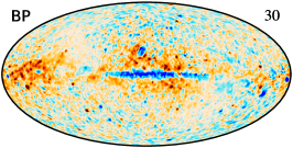
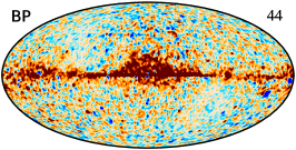
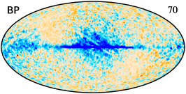
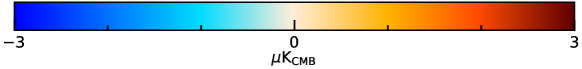
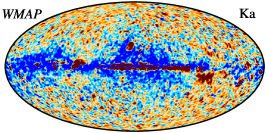
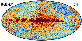
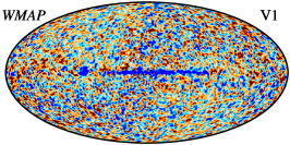
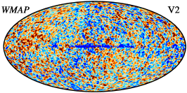
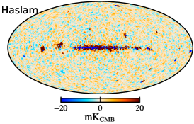
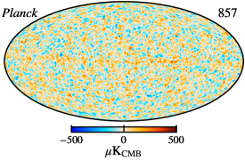
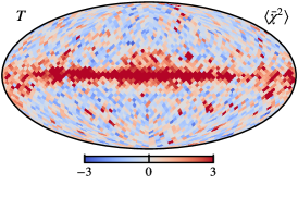
Figure 18: Mean residual maps for the different frequency channels included in the BeyondPlanck analysis. All maps have been smoothed to a common angular resolution of 2^∘ FWHM. The Planck LFI residuals are plotted with a range of 3  $\mu$K_CMB, and the WMAP residuals are plotted with a range of 5  $\mu$K_CMB. The bottom right panel shows the mean reduced chi-squared $\bar{\chi}^{2}$ per $N_{\mathrm{side}}=16$ pixel of the BeyondPlanck Gibbs chain.

Before presenting the actual posterior distributions, we consider the goodness-of-fit of the derived model. First, Fig. 18 shows posterior mean residual maps on the form $\@vec{r}_{\nu}=\@vec{d}_{\nu}-\@vec{s}_{\nu}$ for each of the ten frequency bands included in the analysis, where the average is evaluated over all samples in the Markov chain.

Starting with the LFI channels shown in the top section of the figure, we see that the residuals at high Galactic latitudes are largely consistent with instrumental noise, except for scattered point source residuals at 30 GHz, while at low Galactic latitudes there is an obvious dust morphology residual coming from either AME or thermal dust. At 30 GHz it is also possible to see some bright negative free-free residuals. Overall, though, the fits are performing quite well, with typical residuals smaller than 3 $\mu$K over most of the sky, and the remaining artefacts are relatively easy to mask through Galactic and point source thresholding.

The middle section shows the WMAP channels, plotted on a color range of $\pm 5\thinspace\mu\mathrm{K}$. The most striking residual feature in this case is a strong dust residual in the Ka (33 GHz) channel. This, combined with the weaker dust residuals observed in the LFI channels, strongly suggests that the current single-component AME model adopted for the BeyondPlanck analysis is not a statistically adequate model for the actual AME sky. In fact, this shortcoming was already pointed out by Planck Collaboration X (2016), who introduced a second AME component to fit the full contribution. Doing the same with the current data selection would lead to a massively increased noise level for all derived components, and we instead accept the foreground mismodeling here and we instead simply make sure to mask out the contaminated regions of the sky in higher-order analyses.

Other notable features in the WMAP residuals are large regions of low-level residuals at high Galactic latitudes that do not obviously trace known Galactic components. As discussed by Barnes et al. (2003), an important challenge regarding this data set on large angular scales is sidelobe modeling and this may also be relevant for the residuals we see in Fig. 18. A re-analysis of the time-ordered WMAP data within the BeyondPlanck framework is already ongoing (Watts et al. 2022).

The last two frequency channels, Haslam 408 MHz and HFI 857 GHz, show very uniform residuals. This is simply due to the fact that their unique S/N values massively dominate the synchrotron and thermal dust components, respectively, and any potential mismodeling would therefore leak directly into the component amplitude maps. A flat residual should thus not be interpreted as the absence of systematic errors, but rather simply as an indication that these two channels have no significant crosscheck in terms of their effect on the signal model by any other channel. We note that this is not entirely true for the Haslam 408 MHz map, which does have competitors in terms of free-free emission near the Galactic center in Planck and WMAP, and corresponding residuals may be seen here.

The bottom right panel of Figure 18 shows the reduced and normalized $\chi^{2}$ per $N_{\mathrm{side}}=16$ pixel, as defined by:

$$\bar{\chi}^{2}(p)=\frac{\sum_{\nu,p^{\prime}\in p}\left[\frac{d_{\nu}(p^{\prime})-s_{\nu}(p^{\prime})}{\sigma_{\nu}(p^{\prime})}\right]^{2}-n_{\mathrm{dof}}}{\sqrt{2n_{\mathrm{dof}}}},$$ (32)

where the sum runs over all pixels within a given low-resolution pixel, and $n_{\mathrm{dof}}=15\thinspace 400$ is an estimate of the total number of degrees of freedom for each low-resolution pixel. Since $n_{\mathrm{dof}}$ is large, this quantity is expected to be $N(0,1)$ distributed in the ideal case, and Fig. 18 thus quantifies the agreement between the data and the model in units of standard deviations per pixel. Overall, we see that the distribution agrees with the expectation to about $1\thinspace\sigma$ at high Galactic latitudes, except for some compact sources, while at low Galactic latitudes there is a strong residual with a clear dust-like morphology. This $\chi^{2}$ map serves as an important input for producing masks for higher order analyses.

6.4 Signal component posterior distributions

Table 3: Comparison of frequency channel monopole constraints from BeyondPlanck and Planck. For Planck, all numbers correspond to the Planck 2015 analysis (Planck Collaboration X 2016), except for the HFI 857 GHz, which is taken from Planck DR4 (Planck Collaboration LVII 2020). We note that the Planck 2015 analysis did not fit for the WMAP Ka-band monopole, but fixed it at the given value; this parameter therefore has no associated uncertainty. Lastly, we note that while the WMAP and HFI maps are the same in both columns, the LFI maps are not, and they have different zero-levels coming from the TOD processing.

Channel	BeyondPlanck	Planck	Unit
LFI 30 GHz	$0\pm 6$	$-17\pm 1\phantom{-0}$	$\mu\mathrm{K_{CMB}}$
LFI 44 GHz	$0\pm 2$	$\phantom{-}11\pm 1\phantom{-0}$	$\mu\mathrm{K_{CMB}}$
LFI 70 GHz	$0\pm 1$	$\phantom{-}16\pm 1\phantom{-0}$	$\mu\mathrm{K_{CMB}}$
WMAP Ka	$16\pm 3\phantom{-}$	$3$	$\mu\mathrm{K_{CMB}}$
WMAP Q1	$12\pm 2\phantom{-}$	$\phantom{-}2\pm 1\phantom{-0}$	$\mu\mathrm{K_{CMB}}$
WMAP Q2	$11\pm 2\phantom{-}$	$\phantom{-}2\pm 1\phantom{-0}$	$\mu\mathrm{K_{CMB}}$
WMAP V1	$6\pm 1$	$\phantom{-}1\pm 1\phantom{-0}$	$\mu\mathrm{K_{CMB}}$
WMAP V2	$6\pm 1$	$\phantom{-}1\pm 1\phantom{-0}$	$\mu\mathrm{K_{CMB}}$
HFI 857 GHz	$-0.65\pm 0.03\phantom{-}$	$-0.72\pm 0.01\phantom{-0}$	$\phantom{\mu}\mathrm{K_{CMB}}$

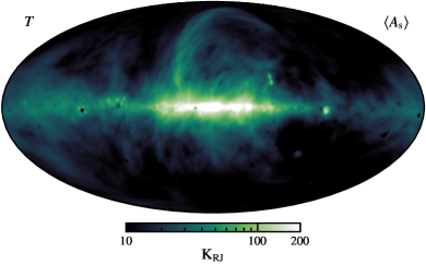
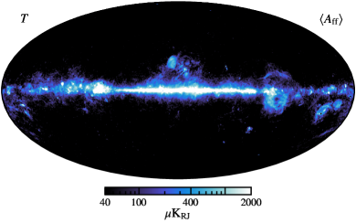
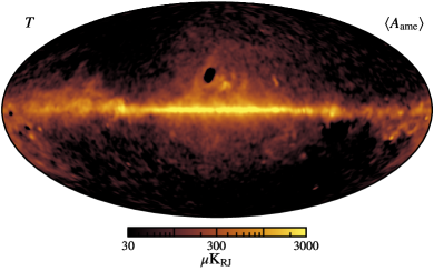
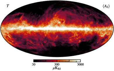
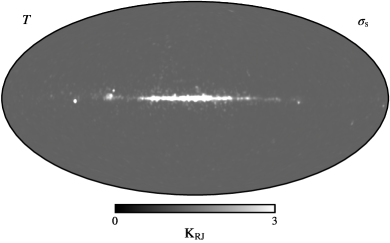
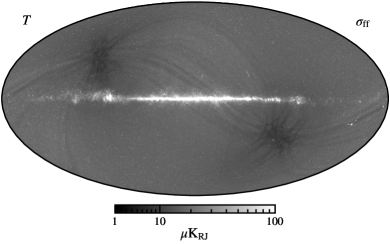
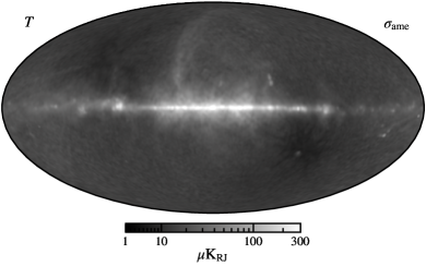
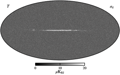
Figure 19: Posterior mean amplitude maps for each of the four fitted foreground component; synchrotron (top-left), free-free (top-right), AME (bottom-left), and thermal dust emission (bottom-right). The angular resolutions of the four maps are 120, 30, 120, and 10^′ FWHM, respectively.

Figure 20: Posterior standard deviations for the same maps as shown in Fig. 20. We note that synchrotron and dust emission are potted with linear scaling.

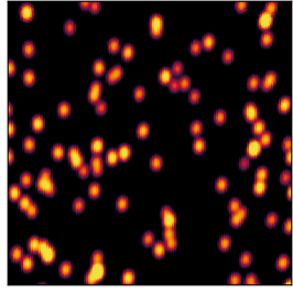
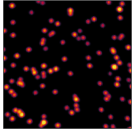
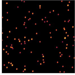
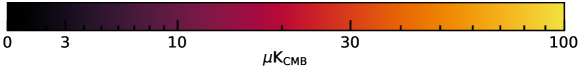
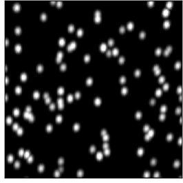
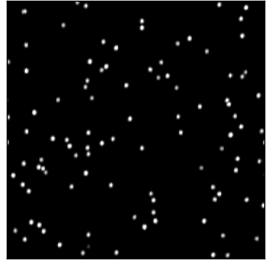
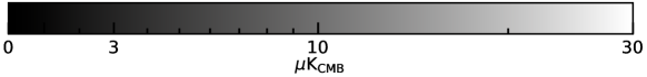
Figure 21: Partial sky plots of the mean (top) and standard deviation (bottom) amplitude of the fitted compact sources (point sources) as seen by the three Planck LFI detector bands; 30 GHz (left), 44 GHz (middle), and 70 GHz (right). The plots show gnomonic projections of a $20\times 20$ degree patch of the sky centered on 90^∘ longitude and 70^∘ latitude, with the north galactic pole located towards the top-center of the plots. All plots are at native angular resolution and pixelization, see Table 1 for details.

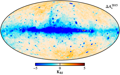
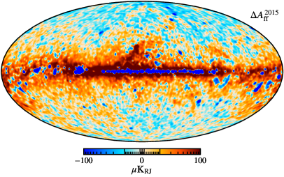
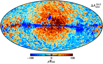
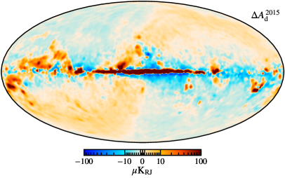
Figure 22: Difference maps between the component amplitude maps derived in BeyondPlanck and the Planck 2015 analysis, for synchrotron (top-left), free-free (top-right), AME (bottom-left), and thermal dust emission (bottom-right), respectively. All maps have been smoothed to a common angular resolution of 2^∘ FWHM, a relative offset has been fitted and subtracted using the frequency-band monopole mask discussed in Sect. 4.3 and differences in reference frequencies (where relevant) have been accounted for by a single multiplicative scaling factor.

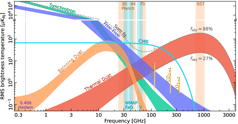
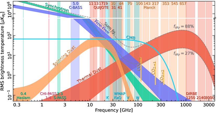
Figure 23: Brightness temperature RMS as a function of frequency and astrophysical component for temperature. Each component is smoothed to an angular resolution of 1^∘ FWHM, and the lower and upper edges of each band are defined by masks covering 27 and 88 % of the sky, respectively. We note that foreground RMS values decrease nearly monotonically with sky fraction, whereas the CMB RMS is independent of sky fraction, up to random variations. The vertical bands represent the frequency range of detector data, where the top panel shows the data employed in this paper and the bottom panel shows some data available for future analysis.

Next, we consider the signal component posterior distributions and we start with the frequency monopoles, as summarized in terms of posterior mean and standard deviations in the second column of Table 3. For comparison purposes, the third column shows corresponding results derived by the Planck team; all results except 857 GHz are reproduced from the Planck 2015 analysis (Planck Collaboration X 2016), while the 857 GHz result is taken from Planck DR4 (Planck Collaboration LVII 2020).

Several important differences between the two sets of results can be identified. First, we note that the BeyondPlanck LFI mean monopoles are all zero; this happens by construction during the mapmaking process, as the frequency band monopoles are determined directly from the sky model and any deviation from this is assigned to the correlated noise component (Ihle et al. 2022). On the other hand, we do see that the uncertainties of the LFI zero-levels are larger at both 30 and 44 GHz, reflecting the difficulty of uniquely determining the AME offset, as discussed in Sect. 4.2. In addition, the uncertainty of the Haslam, and thereby the synchrotron monopole propagates down to the lower frequency Planck and WMAP channels and contributes to increased uncertainties of these monopoles. We argue that the uncertainties determined through component-based monopole determination are more realistic than those obtained through morphologically based frequency monopole determination.

For WMAP, we note that the our monopole corrections are considerably larger compared to those determined in the Planck 2015 estimates. This is caused by two main differences. First, the 2015 analysis adopted the WMAP Ka-band explicitly as a fixed “anchor channel” (Planck Collaboration X 2016) that was not allowed to vary in the analysis. In the current analysis, for which we instead impose constraints directly on the component monopoles, this channel is instead associated with a $16\thinspace\mu\mathrm{K_{CMB}}$ correction, which is then accounted for by an offset of $-17\thinspace\mu\mathrm{K_{CMB}}$ at LFI 30 GHz in the 2015 analysis. Second, we have changed the average synchrotron index from $\beta_{\mathrm{s}}=-3.1$ in the Planck 2015 analysis (Planck Collaboration X 2016) to $\beta_{\mathrm{s}}=-3.3$ in the current analysis. Since the synchrotron monopole is set to 8.9  K_RJ at 408 MHz (see Sect. 3), the predicted monopole at WMAP Ka-band is 11 $\mu$K_CMB with $\beta_{\mathrm{s}}=-3.1$ and 4 $\mu$K_CMB with $\beta_{\mathrm{s}}=-3.3$, a difference of 7 $\mu$K_CMB. The frequency band monopole has to adjust for this difference. Similarly, differences in the zero-level of the other components, especially the AME, will contribute to frequency-band monopole differences in equal fashion. Regarding the offsets for the 857 GHz channel, we see that these agree within $2\thinspace\sigma$ as estimated by BeyondPlanckand the uncertainties are significantly larger (and, we believe, more realistic) in the new approach, which is a reflection of the fact that we are now propagating uncertainties in the thermal dust zero-level as discussed in Sect. 4.2.

Regarding spectral parameters, the AME peak frequency is the only spectral parameter that is fully sampled from the data in this component separation work. For this, we find a posterior mean and standard deviation of $\nu_{\mathrm{p}}=25.3\pm 0.5\thinspace\mathrm{GHz}$. From the high correlation coefficient between $\nu_{\mathrm{p}}$ and the thermal dust $\beta_{\mathrm{d}}$ seen in Fig. 17, it is clear that this result is highly dependent on the assumptions made regarding thermal dust modeling in this paper, and future work that includes Planck HFI observations will be critically important to make the AME model more robust.

Posterior mean and standard deviation maps for each of the four component maps (synchrotron, free-free, AME, and thermal dust emission) are shown in Figs. 20 and 20, each at their own angular resolution (120, 30, 120, and 10^′) and reference frequency (408 MHz, 40 GHz, 22 GHz, and 857 GHz), and all shown in terms of brightness temperature. In Figure 20, we notice the dark stripes following the Planck scanning pattern at high galactic latitudes in the standard deviation map of the free-free component. These stripes are barely visible in the AME standard deviation map while being completely absent from the synchrotron and thermal dust maps. This can be explained by the sampling of the amplitude zero-levels, where the free-free zero-level is the only one not marginalized over in the BeyondPlanck Gibbs chain. The base value at higher latitudes of the amplitude RMS is equivalent to the RMS of the sampled zero-levels.

Figure 21 shows mean and standard distribution plots for the compact source component for a $20^{\circ}\times 20^{\circ}$ field of the sky in the Northern Galactic hemisphere for each of the three LFI frequency channels. The four-component posterior mean maps may be compared to similar products from the Planck 2015 analysis (Planck Collaboration X 2016) and corresponding difference maps are shown in Fig. 22. All maps are smoothed to a common angular resolution of $2^{\circ}$ FWHM before differencing, and a free offset has been fitted and subtracted using the frequency-band monopole mask discussed in Sect. 4.3. In addition, for the components that have different reference frequencies in the two analyses (i.e.., free-free, AME, and thermal dust emission), a single multiplicative factor has been fitted to take into account SED scaling differences.

Starting with the synchrotron case, we note that typical high-latitude differences are small compared to the overall amplitude of the Haslam 408 MHz map, typically less than $1\thinspace\mathrm{K}_{\mathrm{RJ}}$. This is of course entirely expected, since the two analyses are both dominated by the same map. However, we do see differences at both low and high Galactic latitudes; for high latitudes we note that the current analysis explicitly models individual point sources, while in the Planck 2015 analysis there was no such component and compact sources were therefore part of the diffuse components. At low latitudes, the differences are dominated by differences in the free-free, AME, and thermal dust emission models.

For free-free emission, we see clear negative imprints of the free-free amplitude map itself at low Galactic latitudes. In this case, we note that while the Planck 2015 analysis fit the electron temperature pixel-by-pixel, we adopt a single constant value of $T_{e}=7000\thinspace\mathrm{K}$ in the current analysis. Second, we see clear positive imprints of AME or dust around the negative free-free imprint at low Galactic latitudes, resulting from degeneracies between the component signals. Lastly, we also note that the current analysis suffers significantly with respect to free-free emission due to the absence of the Planck HFI channels, which provide both angular resolution and sensitivity to this component.

The AME component residual map is largely dominated by a dipole component aligned with the direction of the Galactic center. In this case, we note that the BeyondPlanck analysis estimates the absolute calibration of each Planck LFI frequency channel through a joint fit with all frequencies and this provides more robust estimates of the CMB dipole. We also see a negative free-free imprint at low Galactic latitudes similar to what we see in the free-free difference map. One key feature is the almost circular blob just above and slightly to the left of the Galactic center, which is also clearly seen as a dark blob in the mean map in Fig. 20. This coincides with a similarly bright circular blob in the free-free amplitude. A similar signal can be seen in the Planck 2015 free-free signal (Planck Collaboration X 2016), although it did not affect the AME amplitude in the same way. If we look at the residuals in Fig. 18, we notice the same blob in the LFI 30 GHz and the WMAP $Ka$ maps, indicating a degeneracy between the modeled AME and free-free components. To break this degeneracy, either more data sets needs to be introduced or the free-free $T_{\mathrm{e}}$ and the AME $\nu_{\mathrm{p}}$ needs to be sampled with spatial variance, or both. This is, however, not possible with the limited data set in this analysis and therefore needs to be left for future analyses.

Finally, for the thermal dust emission amplitude map, which is essentially defined by the Planck 857 GHz frequency map, the differences are explained very closely by the morphology of the thermal dust spectral index map $\beta_{\mathrm{d}}(p)$ presented by Planck Collaboration X (2016). This is also entirely expected, given the fact that we only model $\beta_{\mathrm{d}}$ in terms of a single spatial constant over the full sky.

7 Summary and outlook

The main goal of the current paper is to establish an efficient Monte Carlo sampling scheme for intensity foregrounds within an end-to-end Bayesian CMB analysis pipeline, as implemented in the BeyondPlanck framework. This sampling scheme must be able to operate in both low and high signal-to-noise regimes, and it must be able to incorporate both algorithmic and informative priors in a controlled and transparent manner. Degeneracies between different parameters must be explored properly and it must be possible to propagate corresponding uncertainties to higher level products.

Most of the algorithmic elements in the machinery used in this paper were developed and applied within the context of the official Planck project, as described in, for instance, Planck Collaboration X (2016), Planck Collaboration IV (2018), and Planck Collaboration LVII (2020). In this paper, we have added four new algorithmic components to this machinery, namely: 1) joint amplitude and spectral index sampling, borrowing heavily from ideas already introduced by Stompor et al. (2009) and Stivoli et al. (2010); 2) component-based monopole determination; 3) joint spectral index and monopole sampling; and 4) the application of informative spatial priors. Each of these steps significantly improve the computational efficiency and robustness of the Gibbs sampling-based Commander approach.

We stress that the current BeyondPlanck results are not intended to define a new state-of-the-art model of the astrophysical sky. Rather, the current framework and analysis constitute a “skeleton” to which additional data sets, both legacy and future, may be added in a controlled fashion, keeping track of both instrumental and astrophysical modeling errors. As more and more data sets are added, the dependency on external priors may be gradually lifted until, hopefully, all key parameters of the model become data driven. Obviously, the single most important step towards realizing this goal is the introduction of Planck HFI TOD observations, which still define the state-of-the-art in terms of full-sky CMB sensitivity to date. On a longer term, we argue that all key data sets in the community should be integrated into the model, allowing one set to break the degeneracies of others. This is the goal of the Open Source Cosmoglobe project, and the transition from BeyondPlanck to Cosmoglobe may be illustrated in Fig. 23: the top panel of this figure shows the standard deviation brightness temperature as a function of frequency for each primary intensity CMB foreground as colored bands. The BeyondPlanck frequency bands are indicated by vertical bars. Looking at this figure, noting the large unexplored frequency ranges, it is strikingly obvious why the current data model is significantly prior dominated; thus, more data are desperately needed. The bottom panel of Fig. 23 shows an alternative scenario, in which almost the entire frequency range is covered by including data from several past and planned sky surveys. Providing a computationally and organizationally efficient platform to make this happen is the goal of Cosmoglobe and the BeyondPlanck project represents an important step towards realizing this promise.