Conditional Generation of Medical Time Series for Extrapolation to Underrepresented Populations

Abstract

The widespread adoption of electronic health records (EHRs) and subsequent increased availability of longitudinal healthcare data has led to significant advances in our understanding of health and disease with direct and immediate impact on the development of new diagnostics and therapeutic treatment options. However, access to EHRs is often restricted due to their perceived sensitive nature and associated legal concerns, and the cohorts therein typically are those seen at a specific hospital or network of hospitals and therefore not representative of the wider population of patients. Here, we present HealthGen, a new approach for the conditional generation of synthetic EHRs that maintains an accurate representation of real patient characteristics, temporal information and missingness patterns. We demonstrate experimentally that HealthGen generates synthetic cohorts that are significantly more faithful to real patient EHRs than the current state-of-the-art, and that augmenting real data sets with conditionally generated cohorts of underrepresented subpopulations of patients can significantly enhance the generalisability of models derived from these data sets to different patient populations. Synthetic conditionally generated EHRs could help increase the accessibility of longitudinal healthcare data sets and improve the generalisability of inferences made from these data sets to underrepresented populations.

1 Introduction

The broad use of electronic health records (EHRs) has lead to a significant increase in the availability of longitudinal health care data. As a consequence, our understanding of health and disease has deepened, allowing for the development of diagnostic and therapeutic approaches directly derived from EHR patient data. Models that utilize rich healthcare time series data derived from clinical practice could enable a variety of use cases in personalised medicine, as evidenced by the numerous recent efforts in this area [22, 42, 44, 49]. However, the development of these novel diagnostic and therapeutic tools is often hampered by the lack of access to actionable patient data [2].

Even after being deidentified, EHR data is perceived as highly sensitive and clinical institutions raise legal and privacy concerns over the sharing of patient data they may have access to [55]. Furthermore, even if data is made public, it often originates from a single institution only [24, 26, 36], resulting in a data set that may not be representative for more general patient populations. Basing machine learning models on single site data sets only risks overfitting to a cohort of patients that is biased towards the population seen at one clinic or hospital, and renders their use for general applications across heterogeneous patient populations uninformative at best and harmful at worst [10, 60].

Putting aside the issue of non-representative patient cohorts, the development of accurate machine learning-based models for healthcare is further impeded by the imbalance in magnitude of the available data compared to other domains. While fields such as computer vision or language modelling have made significant advances, thanks in part to access to large-scale training data sets like ImageNet [9] or large text corpora derived from the World Wide Web, there do not yet exist any comparable data repositories for machine learning in healthcare that may spur innovation at similar pace. Practical problems may also arise during model development due to a lack of training samples for specific, rare patient conditions. If one wishes to study a model’s behaviour given data with certain properties, such as only patients with a certain pre-existing condition, medical data sets may often be too small to representatively cover such populations.

One potentially attractive approach to address the aforementioned issues would be to generate realistic, synthetic training data for machine learning models. Given access to an underlying distribution that approximates that of the real data, paired with the capability to sample from it, one could theoretically synthesize data sets of any desired size. The generated synthetic patient data can be used for assessing [5, 6, 52] or even improving machine learning healthcare based software e.g. for liver lesions classification [16]. If the generative model of the data were to also have the capacity to generate samples conditioned on factors that may be freely chosen, such as for example pre-existing conditions, data sets with the exact properties required for a specified task could be generated as well. Previous reports suggest that such synthetically generated data sets may furthermore be shared with a significantly lower risk of exposing private information [3].

Developing models with synthetic data is already widely applied in machine learning research. In Reinforcement Learning for example, it is the de-facto standard to train models in simulation, in order to have high-fidelity control over the environment [50, 1], or simply because experiments in the real world would be to costly, unethical or dangerous to conduct. Some previous work even suggests that models trained on synthetic data could outperform those derived from real data sets [51]. The gap between real and synthetic data is rapidly closing in fields like facial recognition in computer vision, as has for example recently been demonstrated by Wood et al. [57].

Classical approaches to generating medical time series data exist, but they fall short of the requirements that modern data-driven models require for their input. Some works employ hand crafted generation mechanisms followed by expensive post-hoc rectifications by clinical professionals [3], while others rely on mathematical models of biological subsystems such as the cardiovascular system [34, 37], which require a detailed physiological understanding of the system to be modelled. When the output data stems from multiple, interconnected subsystems whose global dynamics are too complex to model with ordinary differential equations and the size of the required data set is too large to tediously correct unrealistic samples by experts, these approaches may be difficult to utilize.

A natural approach to learning complex relationships from data is to move away from hand-crafted generative models and utilize machine learning methods. While a plethora of powerful generative models for medical imaging data generation have been brought forward in recent years [11, 19, 30, 46], relatively little research has been reported on generating synthetic medical time series data [2, 8, 25, 54]. Moreover, the generation and evaluation of synthetic patient data [20] is often challenging due to the high missingness in the original medical datasets [31, 35, 41, 43].

To address these issues, we present HealthGen, a new approach to conditionally generate EHRs that accurately represent real measured patient characteristics, including time series of clinical observations and missingness patterns. In this work, we demonstrate that the patient cohorts generated by our model are significantly better-aligned to realistic data compared to various state-of-the-art approaches for medical time series generation. We demonstrate that our model outperforms previous approaches due to its explicit development for real clinical time series data, resulting in modelling not only the dynamics of the clinical covariates, but also their patterns of missingness which have been shown to be potentially highly informative in medical settings [4]. We show that our model’s capability to synthesize specific patient subpopulations by means of conditioning on their demographic descriptors allows us to generate synthetic data sets which exhibit more fair downstream behavior between patient subgroups, than competing approaches. Moreover, we demonstrate that by conditionally generating patient samples of underrepresented subpopulations and augmenting real data sets to equally represent each patient group, we can significantly boost the fairness of downstream models derived from the data. Furthermore, we evaluate the quality and usefulness of the data we generate using a downstream task that represents a realistic clinical use-case - allowing us to compare our model against competing approaches in a setting that is relevant for clinical impact.

Our main contributions are:

• We introduce HealthGen, a new machine-learning method to conditionally generate realistic EHR data, including patient characteristics, the temporal evolution of clinical observations and their associated missingness patterns over time.

• We experimentally show that our method outperforms current state-of-the-art models for medical time series generation in synthetically generating patient cohorts that are faithful to real patient data.

• We demonstrate the high fidelity of control over synthetic cohort composition that our model provides by means of its conditional generation capability, by generating more diverse synthetic data sets than competing approaches, which ultimately leads to a more fair representation of different patient populations.

• We show that by augmenting real data with conditionally generated samples of underrepresented populations, the models derived from these data sets exhibit significantly more fair behaviour than those derived from unaltered real data.

• We perform a comprehensive computational evaluation in realistic clinical use cases to evaluate the comparative performance of HealthGen against various state-of-the-art generative time-series modelling approaches.

2 Results

2.1 Overview

For this study, we consider the MIMIC-III data set [26], which consists of EHRs containing time series of measurements of patients that spent time in the intensive care unit (ICU). Additionally, each patient is described by static variables such as their age, ethnicity, insurance type and sex. The time series of a given patient is labelled to indicate whether or not one of the following clinical interventions was performed: mechanical ventilation, vasopressor administration, colloid bolus administration, crystalloid bolus administration or non-invasive ventilation.

After extracting the cohort of patients from the data base, we split them into training (70%), validation (15%) and test (15%) sets, stratified by their binary intervention labels. The generative models are trained on the real training data $\mathcal{D}_{\text{train}}=\{\mathbf{x}^{n}_{1:T},\mathbf{m}^{n}_{1:T},\mathbf{s}^{n},\mathbf{y}^{n}\}^{N_{\text{train}}}_{n=1}$, where $\mathbf{x}_{1:T}$ denotes the time series of covariates, $\mathbf{m}_{1:T}$ the time series of binary masks indicating where values are missing, $\mathbf{s}$ the static patient variables and $\mathbf{y}$ a patient’s set of labels for the respective clinical interventions. We include the missingness information $\mathbf{m}_{1:T}$ explicitly, as previous work has shown that patterns of missing values are highly informative [41] and especially in the medical setting including them is preferential to imputation [4].

To evaluate and compare generative models, we first train a downstream time series classification model developed for medical data [4] on the data sets synthesized by each model. This classifier that has been trained with synthetic data is evaluated on the held-out real test data, and the resulting AUROC score (Area Under the Receiver Operating Characteristic curve) is compared with the AUROC score of the same classifier trained on the real data. The final measure for how faithful a given generated data set is to the real data is the difference between the evaluation score of the synthetic data and that of the real data. Details on the experimental pipeline can be found in Section 4.

In our first experiment, we generate synthetic patient cohorts that are faithful to the real data in terms of their demographics, i.e. they contain the same number of patients as the original data under the same distribution of static variables. Repeating this synthetic cohort generation for all of the available clinical intervention labels, we compare the performance of our model to baseline models for generating clinical time series data. As baselines, we consider Stochastic Recurrent Neural Networks (SRNN) [14] and KalmanVAE (KVAE) [15], both based on variational autoencoders (VAE) [29], and TimeGAN [59], based on generative adversarial networks (GAN) [21]. We then present results of an extension of the previous experiment demonstrating our proposed approach’s conditional generation capability, where we generate patient cohorts with static variable distributions that differ from the real data, and investigate the fairness of models derived from the resulting synthetic data. In an additional experiment, we identify real data settings where some subpopulations of patients have a significantly lower classification score than other patients. Using the the conditional generation capability of our model, we augment the real data with synthetic samples of minority groups and test if this augmentation leads to an increase in the downstream classification score of the previously underrepresented populations.

2.2 Generating synthetic patient cohorts

In the first experiment of this work, we investigate our model’s capability to generate synthetic data that is faithful to the real data and useful in downstream tasks. To study the generative performance of our model and compare it against competing approaches for medical time series generation, we employ the experimental framework described in detail in the Methods section.

Here, we train each generative model conditioned on the real labels $\mathbf{y}$ and then generate a synthetic data set $\hat{\mathcal{D}}$, where the generation is again conditioned on the label of the considered task, to guarantee that the synthetic data shares the same statistics in terms of split between positive and negative labels as the real data. While we could in practice generate as much data as we wish, we synthesize data sets containing the same number of patients as the real data for this experiment, to facilitate a fair comparison between the real patient cohorts and those that have been synthetically generated.

A downstream model for medical time series classification [4] is then trained on the synthetic training data $\hat{\mathcal{D}}_{\text{train}}$ of each generative model and evaluated on a held out test data set $\mathcal{D}_{\text{test}}$ consisting of real patients. We compare the performance of our model against the current state-of-the-art models for time series generation, across all five available classification tasks in the MIMIC-III data. The results of these experiments are summarized in LABEL:tab:synth_gen. We provide examples of synthetically generated patients’ time series in Figure 1, next to a real patient’s time series for comparison. Additional, more detailed visualisations are presented in Appendix D.

In all considered tasks, our approach significantly outperforms the state-of-the-art models in synthetically generating medical time series. The fact that our model’s downstream classification score is higher then the baselines’, across all experimental settings, suggests that the synthetic data generated by our model is more faithful to the real data and thus more useful for the development of downstream clinical time series prediction tasks than the cohorts generated by any of the competing architectures.

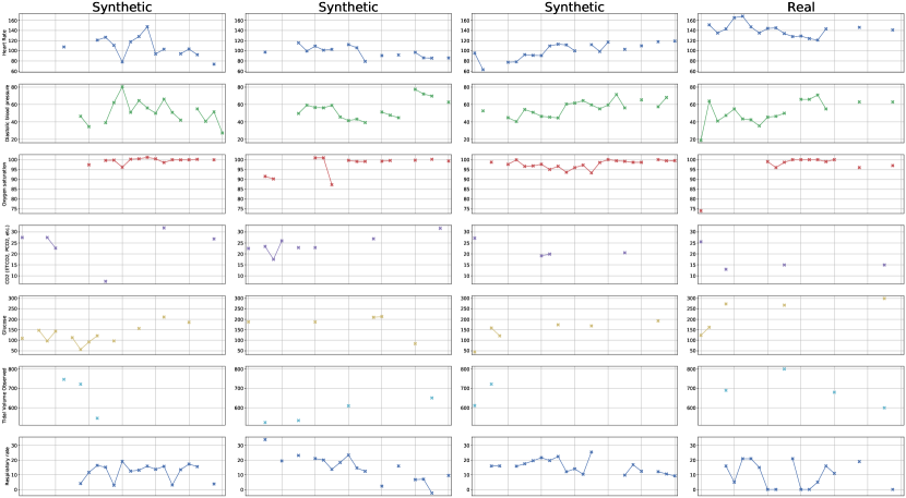
Figure 1: Sample time series of synthetically generated patients, with the time series of one real patient for comparison.

Table 1: Comparison of AUROC scores for all predictive tasks between HealthGen and the baseline models. The 95% confidence interval of the mean value is presented in parentheses and is estimated via bootstrapping with 30 samples.

	vent	vaso	colloid_bolus	crystalloid_bolus	niv
Real Data	0.809 (0.807, 0.811)	0.801 (0.799, 0.803)	0.751 (0.741, 0.760)	0.613 (0.609, 0.616)	0.634 (0.632, 0.637)
HealthGen (Ours)	0.769 (0.767, 0.772)	0.722 (0.718, 0.727)	0.664 (0.650, 0.678)	0.574 (0.571, 0.577)	0.567 (0.566, 0.569)
SRNN	0.639 (0.637, 0.641)	0.693 (0.690, 0.695)	0.661 (0.656, 0.666)	0.562 (0.561, 0.564)	0.553 (0.552, 0.555)
KVAE	0.559 (0.549, 0.570)	0.608 (0.589, 0.627)	0.565 (0.544, 0.586)	0.538 (0.531, 0.545)	0.523 (0.517, 0.529)
TimeGAN	0.558 (0.558, 0.558)	0.703 (0.703, 0.704)	0.552 (0.530, 0.573)	0.545 (0.543, 0.548)	0.530 (0.527, 0.533)

2.3 Conditional generation

From Table C.3 we see that many demographic variables have examples of highly underrepresented classes, possibly leading to the classification performance for these subpopulations to be much lower than for the majority class. This shines a light on a real problem found in many clinical settings, especially when transferring between hospitals [44]. In preliminary experiments, we investigate the classification score on a per-group level for the real data. While it does not occur for all static variables and classification tasks, we identify cases where there is a significant difference in the score of a given subpopulation, with respect to the other groups. This inter-group performance gap raises the question if our model’s conditional generation capability can be leveraged to address these fairness issues.

In the preceding experiment, we do no utilize our model’s capacity to conditionally generate synthetic patient cohorts, as we do not explicitly condition our model on the static variables $\mathbf{s}$ during training or generation. Here, in addition to the label $\mathbf{y}$, we condition on a static variable of interest allowing us to then conditionally generate an equal number of synthetic patient samples for each subgroup of this considered static variable. We investigate if conditionally generating patient cohorts provides a benefit in terms of fairness, as well as overall downstream performance. In this experiment, we study the performance on a per-group level, comparing not only to the baseline approaches, but to our model when unconditionally generating the data, as well. To enable a fair comparison, the overall number of generated patients is equal for each considered model. The results of this experiment for two exemplary settings are presented in Figure 2, with additional results reported in Section A.3.

The results indicate that, for settings in which the real data exhibits performance differences between subpopulations, conditonally generating synthetic patient cohorts provides a significant benefit over unconditional generation. In terms of overall performance, and in nearly all subgroups, our model outperforms the baselines when conditionally generating data. The variance of the scores across groups is also smaller when conditionally generating, than for any of the competing approaches. Our model is not only capable of generating synthetic “copies” of the real data in terms of the distribution of demographics, but we can generate data sets with a high degree of control over the composition of subpopulations, resulting in more diverse training sets for downstream tasks.

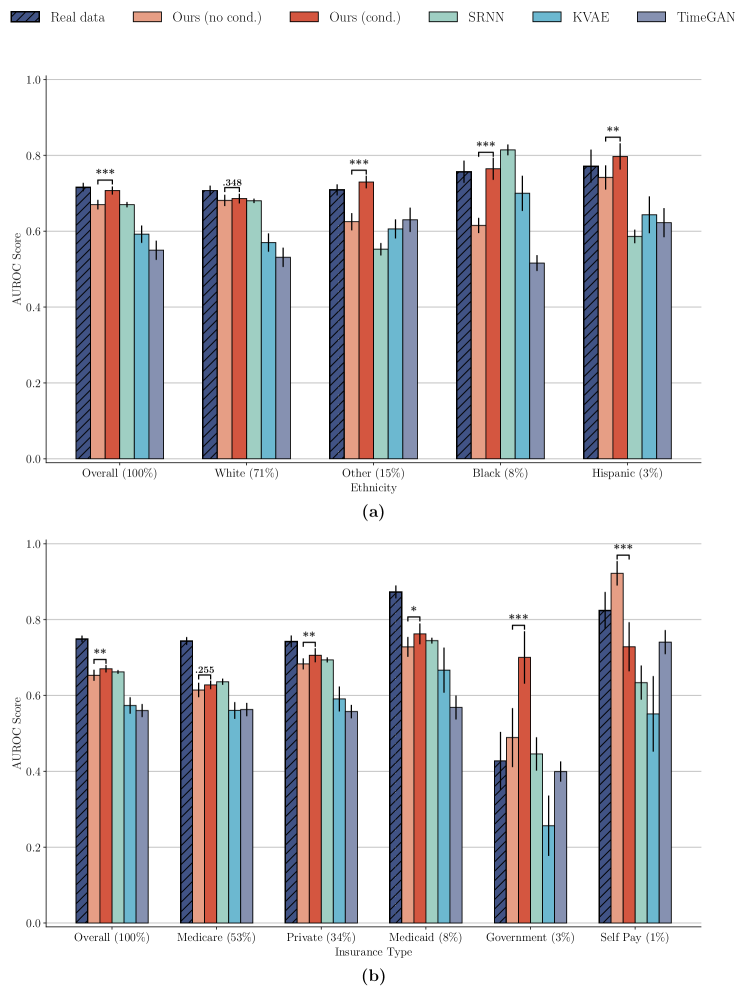
Figure 2: Comparison of AUROC score between our model when conditionally and unconditionally generating synthetic data with baselines. We show results of the colloid_bolus task for different ethnicity groups (a) as wells as the range of insurance types (b). Note that the Asian subpopulation is not among the ethnicity groups, as there are no positive samples among this group for the considered task, thereby prohibiting the calculation of the AUROC score. Conditionally generating patient cohorts is favourable to unconditional generation overall, and for almost all subgroups, allowing for the generation of more representative and therefore fair synthetic data sets. Significance levels between groups of interest are shown with brackets, where * corresponds to p $<$ 0.05, ** to p $<$ 0.01 and *** to p $<$ 0.001

2.4 Real data augmentation

In the preceding experiment, we demonstrated that our model’s conditional generation capability can be used to synthesize patient cohorts that yield more fair downstream classification models. The settings that emerge in which our model can provide a benefit are those where the real data displays an imbalance in the downstream performance between patient subpopulations. This gives rise to the question if our approach to conditionally generate synthetic data can also be useful for the setting when access to the real data is not restricted, but rather the given cohort does not fulfill the requirements for the development of downstream models. For these cases, we hypothesize that we can conditionally generate more examples of this previously underrepresented class, augment the real data with them and thereby boost the performance in the downstream classification task for this subpopulation.

One of the cases, where we identify a significant difference in the performance of the trained classifier for different subtypes of patients, is the colloid_bolus classification task when looking at different insurance types of patients. In Figure 3, we see that while the overall score on this task is fairly high, the underrepresented class of Government insured individuals has a significantly lower score than all other classes. The score of this class is even lower than 0.5, which would be obtained by randomly guessing which class a sample belongs to.

To investigate if our model can improve the performance for such an underrepresented group, we conditionally generate additional samples of each underrepresented class and augment the real training data with these until all insurance types are fairly represented by the same number of samples. Since the baselines cannot generate data conditioned on static variables, we have them unconditionally generate the same number of overall samples that our model augments the real data with. We then compare the results of the downstream classifier trained on data sets augmented by synthetic data of the respective generative models to the classifier trained on the real data.

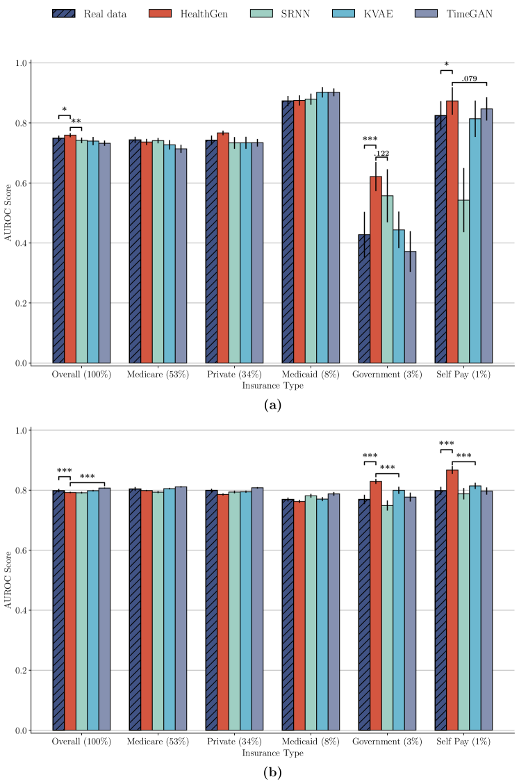
Figure 3: Comparison of the AUROC score between the real data and data sets obtained from the augmenting the real data with the synthetic patients from the considered generative models. We report the scores for each different insurance type on the (a) colloid_bolus as well as the (b) vaso classification task. Significance levels between groups of interest are shown with brackets, where * corresponds to p $<$ 0.05, ** to p $<$ 0.01 and *** to p $<$ 0.001

As we see in Figure 3(a), our model can indeed increase the performance of previously underrepresented groups. Our model significantly boosts the predictive score of the Government class, without sacrificing the performance of any other subpopulation. Interestingly, the performance of the Self Pay class, which is also heavily underrepresented, is also boosted, even if it was already at a high level to begin with. While some other baselines also manage to boost the score of the Government insured class, they either fail to do so to the same degree as our approach, or they also decrease the performance for another class. Our model’s superiority is further demonstrated by the fact that our conditional augmentation leads to a boosting of the overall score as well.

A second setting in which our model provides a benefit for underrepresented classes is the vaso task, again looking at different insurance types. Here, the performance on the minority groups of Government and Self Pay insured patients is not as dramatically lower compared to the other majority groups, but our approach to augment the real data still provides a significant benefit. Visualized in Figure 3(b), our augmentation boosts the performance of the downstream classifier for the two smallest classes significantly, even in a setting where their score is not severely below that of the larger groups to begin with.

2.5 Privacy

To qualitatively assess if our model simply memorizes the training data and reproduces it at generation time, we visualize time series of a randomly selected, synthetically generated sample and time series of the three closest samples (nearest neighbours) in the training data. In Figure 4, we compare the corresponding features of the synthetic and real samples side-by-side and observe that while certain patterns are shared, the synthetic data is not a copy of any of the real patients. This indicates that our model does not memorize the sensitive training data, allowing us to conjecture that it is privacy preserving to a certain degree, and sharing synthetically generated patient cohorts does not jeopardize the private information of the real patients our model was trained with.

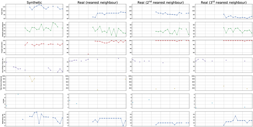
Figure 4: Comparison of the time series of a randomly sampled, synthetically generated patient and the corresponding time series of the three closest real patients (nearest neighbours) in the training data. While certain characteristics such as the number of missing values per feature or dynamics are similar between the synthetic sample and its nearest neighbours amongst the real data, we observe that the synthetically generated data is not a copy of the real data, indicating that our method does not memorize the data it sees during training.

3 Discussion

We presented HealthGen, a deep generative model capable of synthesizing realistic patient time series data, including informative patterns of missingness, that is faithful to data observed in real patient cohorts. To study the quality of the generated patient cohorts, we trained our generative model on the MIMIC-III data set, consisting of labeled ICU patient time series, to synthetically generate EHR data and evaluate the utility of the generated data on the clinically relevant downstream task of classifying patients’ medical time series. In an experimental comparison against existing state-of-the-art models for time series generation, we explored multiple dimensions of the generative capability of our proposed approach: first, we synthesized patient cohorts with the same distribution of static variables as the real training data and observed that the data generated by our model is significantly more faithful to the real data across all evaluated downstream clinical prediction tasks than existing state-of-the-art approaches. In a second experiment, we demonstrated that HealthGen is capable of conditionally generating synthetic patient cohorts with static variable distributions that differ from the underlying, real data, without sacrificing the quality of the generated samples and boosting the fairness of the resulting synthetic patient cohorts. Finally, we identified settings where HealthGen can alleviate issues of unfair downstream classification performance between demographic subpopulations that arise in the real data, by augmenting the real patient cohorts with more diverse, synthetic samples.

3.1 Generating synthetic patient cohorts

A key motivation behind synthetically generating medical time series is the lack of access to this type of data for the development of downstream tasks. Data-driven approaches to assist clinical practitioners in diagnostic or therapeutic tasks promise significant improvements to the quality of healthcare we can provide in the future, but without sufficient data, both in terms of amount and quality, their development is impeded. Clinical institutions that collect this type of data at large are reluctant to centralize and share it, raising the question of how access to useful training and development data may be ensured. One approach that has been brought forward recently is the idea of synthesizing patient cohorts, with the hope that these generated data sets can then be shared freely. In this scenario, only one model hast to be granted access to the sensitive real data, while the synthesized cohorts that are generated by the trained generative model can be freely shared with anyone in need of data for developing a downstream task. The primary requirement for this generated data is that it must adhere to the characteristics of the real data in such a way that it allows for the meaningful development of downstream models. These models are then deployed in the real world, to be used with real data. We demonstrate our model’s capacity to fulfill precisely these requirements. On five different clinical downstream tasks, the synthetic patient cohorts generated by our approach are closer aligned to the real data, evident from their classification scores being closer to that of the downstream task trained on real data, than any competing baselines. While in no setting the generated data ever outperforms the real data in terms of classification score, we stress that this cannot be expected and more importantly this does not diminish the obtained results. In practice, one would only have access to synthetic data for development of these downstream models, so the performance obtained by training on real data is only considered for model selection of the upstream generative model, by means of providing a point of reference for comparison.

Our approach to synthetically generate realistic and useful medical time series data outperforms competing state-of-the-art models for a number of reasons. We include inductive biases aligned with the healthcare domain, in the form of explicitly modelling missing data patterns and separating the generation of these missing values from the generation of observable clinical variables. Furthermore, our model’s capability to capture the influence of static and demographic variables on the generated data and to condition on them during the generation of the synthetic data adds to the expressive capacity of our architecture. To the best of our knowledge, no other models to generate time series in the medical domain explicitly model missing data patterns, even though their importance and prevalence in clinical data is well known. Instead of cherry picking features with low missingness or downsampling the temporal resolution of the data to alleviate missing values, we can generate time series data that is faithful to the characteristics of realistically occurring EHR data. Not only do we outperform the competing baselines on all of the considered downstream tasks, but we do so in a much more realistic setting than previously presented in the literature. This is a notable contribution, as we validate and compare models to generate medical time series with real-world downstream tasks for healthcare applications, giving our findings significantly more weight for clinical practitioners concerned with an impact beyond exemplary academic settings.

3.2 Conditional generation

In the context of healthcare applications, providing fair diagnostic models is of high ethical importance and increasing the fairness of such tools can have a potentially large impact. If an approach works well for the majority of a cohort at the cost of neglecting a certain subclass this can lead to systematically worse treatment of patients belonging to this group. Even a small increase in the predictive quality of a diagnostic tool can mean that hundreds or thousands of patients receive a treatment better aligned with their needs.

In addition to our model being able to generate synthetic patient cohorts of high quality and usefulness, we can do so with a high fidelity of control over the composition of cohorts, without having to sacrifice the quality of the generated data. In settings where the real data displays significant differences in performance between different subpopulations, utilizing this conditioning capability provides a benefit and yields more fair synthetic data sets. This increased fairness is evident from the lower variance between subpopulations when utilizing conditioning, compared to the unconditionally generated data of the other approaches. Importantly, this increase in fairness does not come at the cost of diminishing the performance of certain populations, but rather through an increase in the score of previously sub-par groups, which is also evident in the increase in overall score, with respect to our model when we do not condition. While conditional generation never hurts overall, we cannot boost the score of any subpopulation in any arbitrary setting. For the conditioning to provide a benefit, the real data must display performance imbalances between subpopulations. When this imbalance is not present and all subgroups perform similarly, conditioning should not be expected to provide an additional benefit, as the differences in subpopulations are not relevant for their classification.

The fact that we can successfully condition the generative process of our model to synthesize patients with given features indicates HealthGen’s capability to correctly capture meaningful dependencies between high-level, time invariant patient features and their influence on the resulting dynamics of the generated covariates. The key modelling choices that enable this level of conditioning are the fact that we introduce an additional static latent variable to capture time invariant patient states, as well as the inference procedure by which our model learns the dependencies between this time-invariant latent variable and the dynamics of the sequential data we are interested in generating. Splitting the high-level patient features from the dynamics on an architectural level encourages our model to focus on learning these concepts separately. Independence however does not follow from this separation, as high-level patient states will dictate the evolution of dynamical variables over time, which we capture in the dependencies of the static latent variable on time-varying observations during inference and vice versa during generation.

3.3 Real data augmentation

We have shown that by leveraging our model’s conditional generation capability, we can synthesize data sets which are significantly more fair in their representation of subpopulations of patients. Having demonstrated this in the setting where access to the real data is not given for the development of downstream models, therefore having to rely on fully synthetic data, the question arises if conditionally generated data can also provide a benefit when we do have access to the real data. In a scenario where access to a real data set is given during the development of such a clinical tool, we investigated if augmenting the real data with synthetic patients of specific, underrepresented subpopulations can help to develop a more fair downstream classifier.

After identifying settings where certain subpopulations display significantly lower classification performances than the majority groups, in our final experiment, we demonstrate our model’s capacity to increase the fairness of these real data sets through augmentation with synthetically generated data. This underlines the usefulness of synthetic data generation for a data augmentation task, which is orthogonal to the original objective of our model, namely generation of fully synthetic patient cohorts. That we can boost the performance of downstream tasks using these mixed-modality data sets consisting of real as well as synthetic data speaks to our model’s capability to generate time series that are true to the real data in their informative characteristics and opens up even more possibilities of utilizing synthetically generated data in relevant, real-world applications.

Here, the effect of our approach’s explicit modelling of static variables of interest and the resulting capability to condition on these becomes even more evident. While other generative models can also boost the classification of individual underrepresented classes through unconditional generation, our model proves to have a decisive advantage. The baselines are bound to generate some examples of the minority classes during generation, but we can generate these with high fidelity in a targeted fashion. The resulting augmented data set that follows from our approach manages to boost the score of underrepresented groups, without sacrificing the previously good score of any other subpopulations, which cannot be said for the baselines against which we compare. While we can provide a benefit via augmentation with generated data in specific settings, this does not hold in general. This implies that we cannot simply hope to boost any subpopulations downstream classification performance by generating more samples of this class. Our findings suggest that two main conditions must be met for augmentation to provide a benefit: the gap between the classification score of the minority group and the other groups must exceed a certain magnitude and the other groups must display a minimum score overall, in order for the model to have informative enough examples to learn from, even if they belong to an other group than the one we are interested in generating.

3.4 Limitations

In this work, we do not provide any strong guarantees on the privacy preserving nature of the generated data sets. While it may be interesting to investigate and extend our model in the future in terms of rigorous differential privacy-preserving guarantees [12], we argue that we still generate synthetic data that is privacy-preserving to certain degree. For example, we provide experimental evidence that our model does not simply memorize the training data and reproduce it to generate synthetic cohorts. Moreover, it has also been shown that training neural network architectures with stochastic gradient descent intrinsically guarantees a certain degree of privacy [23], the extent of which is however still an open research question.

Furthermore, the quality and diversity of the generated data which our model produces is limited by the real data with which it is trained. We cannot hope to generate samples of data which are too far out of the distribution of patients which the model has seen during training. A possible solution to this could be the integration of HealthGen into a federated learning framework as an avenue of future development. The initial motivation to synthetically generate EHR data is the lack of large publicly available data sets, with those that are available being only representative of a specific patient cohort. Training a generative model on multiple cohorts in a privacy preserving, federated fashion has been proposed to increase the diversity of the generated data and further catalyze the development of personalized medicine [40, 45].

4 Methods

4.1 Data set and preprocessing

In our experiments, we use the publicly available Medical Information Mart for Intensive Care (MIMIC-III) data set [26] as input. In its raw form, it consists of the deidentified electronic health records (EHRs) of 53,423 patients collected in the intensive care units (ICUs) of the Beth Israel Deaconess Medical Center in Boston, Massachusetts, USA between 2001 and 2012. It consists of multiple tables containing the data of its over 50,000 patients. A single patient’s information is linked across tables through a unique patient ID, and time series data contains a time stamp to maintain the correct temporal ordering of measurements. In this form, the sequential data is not ordered and many of the raw measurements represent the same concept, but are redundantly recorded under different names.

As a first preprocessing step, we employ a slightly modified version of the MIMIC-Extract pipeline [56]. This yields a data set containing the ordered time series of measurements of each patient, static patient variables such as age, sex, ethnicity and insurance type, and a sequence of binary labels at each time step, indicating whether a certain medical intervention was active or not. We apply the standard cohort selection found in the literature [17, 33, 38]: the first ICU admission of adult patients (at least 15 years old), with a minimum duration of at least 12 hours, resulting in a total number of $N=34472$ patients.

At this point, the time series data is still irregularly sampled and asynchronous across different features of the same patient. Given a sampling frequency, we look at the resulting window around each time step and either record the measurement, or indicate the absence of a measurement with a NaN value. We then truncate all time series to have the same, fixed length. In our setting we choose a sampling frequency of 4 steps per hour and truncate the sequences to have a total duration of 12 hours.

From the observed feature sequences we additionally extract a sequence of binary masks $\mathbf{m}_{1:T}$ indicating where a value in $\mathbf{x}_{1:T}$ is missing:

$$m_{t,d}=\begin{cases}1,&\text{if }x_{t,d}\neq\texttt{NaN},\\ 0,&\text{otherwise}.\end{cases}$$ (1)

Finally, we standardize all (non-missing) numerical values of $\mathbf{x}_{1:T}$ to empirically have zero mean and unit variance along each dimension $d\in D$, and replace the NaN values in $\mathbf{x}_{1:T}$ with zeros.

To obtain a binary label for a patient, we split the 12-hour sequence into three sections: a 6-hour observation window followed by a 2-hour hold-out section and finally a 4-hour prediction window. The label is then extracted from the prediction window: if an intervention is active at any time in this section, the label is positive, otherwise it is negative. Drawing inspiration from Suresh et al. [48], this procedure aims to create a fair prediction of future interventions from observed data by minimizing information leakage. If there is no gap between observation and prediction, oftentimes the last step of the observation contains enough information for a meaningful prediction. We extract five binary labels corresponding to different types of clinical interventions in the ICU: vent refers to mechanical ventilation, vaso to the administration of vasopressor drugs, colloid_bolus and crystalloid_bolus refer to colloid and crystalloid fluid bolus administration, respectively, and niv denotes non-invasive ventilation. An overview of the prevalence of overall positive samples for each of these labels is presented in Table C.2. Table C.3 provides a summary of the extracted static variables and the representation of each sub-cohort and LABEL:tab:mimic_stats presents all extracted time-varying features together with selected statistics.

After preprocessing, each patient is represented by a time series of inputs $\mathbf{x}_{1:T}=\{\mathbf{x}_{t}\in\mathbb{R}^{D}\}_{t=1}^{T}$, a time series of missingness masks $\mathbf{m}_{1:T}=\{\mathbf{m}_{t}\in\{0,1\}^{D}\}_{t=1}^{T}$, where $D=104$, a vector of static features $\mathbf{s}\in\mathbb{R}^{M},M=4$ and a set of binary outcome labels $\mathbf{y}\in\{0,1\}^{L},L=5$. The time series $\mathbf{x}_{1:T}$ and $\mathbf{m}_{1:T}$ cover 6 hours of measurements at a resolution of 15 minutes between steps, resulting in a sequence of length 25. The final data set $\mathcal{D}=\{\mathbf{x}^{n}_{1:T},\mathbf{m}^{n}_{1:T},\mathbf{s}^{n},\mathbf{y}^{n}\}^{N}_{n=1}$ is then split into a training, validation and test set, stratified with respect to the labels $\mathbf{y}$.

In Figure 1 we visualize an exemplary set of time series of one patient. We can observe that some covariates such as the heart rate or oxygen saturation have many successive measurements and their evolution over time can be directly studied, while others such as CO2 are missing values at the majority of the time steps and the signal of their dynamics is much sparser. This visualization also shows the two types of correlations evident in the sequential data. Firstly, values of variables may be correlated over time, as we can see from the evolutions of the heart rate and the diastolic blood pressure. Secondly, when values were measured may correlate as well, i.e. the patterns of missingness for different input variables can be related.

4.2 The HealthGen Model

Here we introduce the main technical contribution of this work: the generative model we propose for the task of conditionally generating medical time series data, which we christen HealthGen. The HealthGen model consists of a dynamical VAE-based architecture that allows for the generation of feature time series with informative missing values, conditioned on high-level static variables and binary labels.

As discussed in the previous section, our data consists of a feature time series $\mathbf{x}_{1:T}$ representing the physiological state of a patient, a sequence of binary missingness masks $\mathbf{m}_{1:T}$ indicating when a value of $\mathbf{x}_{1:T}$ is observed and when it is missing, static observable variables $\mathbf{s}$, and labels $\mathbf{y}$. The pattern of missingness is notably not random, and highly informative, as preliminary experiments have shown (see Appendix A). This result is in line with the findings of Che et al. [4], who show that missing values in medical time series play a key role in downstream predictive tasks. The high informativeness of missingness patterns can be explained by imagining a patient with a visibly deteriorating state: clinical staff are much more likely to increase the number and frequency of measurements in this case, compared to a patient whose state is stable. Given their evident importance, we explicitly model the missingness masks $\mathbf{m}_{1:T}$ alongside the observed feature sequence $\mathbf{x}_{1:T}$.

Generative model.

The generative process starts from the static latent variable $\mathbf{v}$ with a fixed unconditional prior $p(\mathbf{v})=\mathcal{N}(\mathbf{v};\mathbf{0},\mathbf{I})$. The observed features and missingness masks are then independently generated as follows. The sequence of missingness masks $\mathbf{m}_{1:T}$ is generated from the static latent variable $\mathbf{v}$, conditioned on the static observable variable $\mathbf{s}$ and label $\mathbf{y}$. We do not model this as a dynamical process, but rather generate the entire sequence in one step, and model it with independent Bernoulli distributions:

$$p_{\theta_{\mathbf{m}}}(\mathbf{m}_{1:T}|\mathbf{v},\mathbf{s},\mathbf{y}) =\prod_{t=1}^{T}\prod_{d=1}^{D}\mathrm{Bernoulli}(m_{t,d};\mu_{t,d}),$$ (2)

where the matrix of probabilities $\bm{\mu}\in[0,1]^{T\times D}$ is given by a DNN $d_{\mathbf{m}}(\mathbf{v},\mathbf{s},\mathbf{y})$ with a sigmoid on the last layer.

Figure 5: Probabilistic graphical model of the generative process of HealthGen.

The generation of the observed features sequence $\mathbf{x}_{1:T}$ is based on the SRNN model [14], with additional conditioning on the static latent $\mathbf{v}$, the static features $\mathbf{s}$, and the labels $\mathbf{y}$, inspired by DSAE [58] and the conditional VAE [47]. The generative model for $\mathbf{x}_{1:T}$ is given by:

$$\mathbf{h}_{1} =e_{\mathbf{h}}(\mathbf{0},\mathbf{v},\mathbf{0}),$$ (3)

$$p_{\theta_{\mathbf{z}}}(\mathbf{z}_{1}|\mathbf{h}_{1}) =\mathcal{N}(\mathbf{z}_{1};\boldsymbol{\mu}_{\theta_{\mathbf{z}}}(\mathbf{0},\mathbf{h}_{1}),\text{diag}\{\boldsymbol{\sigma}^{2}_{\theta_{\mathbf{z}}}(\mathbf{0},\mathbf{h}_{1})\}),$$ (4)

$$\mathbf{h}_{t} =e_{\mathbf{h}}(\mathbf{x}_{t-1},\mathbf{v},\mathbf{h}_{t-1})\text{ for }t>1,$$ (5)

$$p_{\theta_{\mathbf{z}}}(\mathbf{z}_{t}|\mathbf{z}_{t-1},\mathbf{h}_{t}) =\mathcal{N}(\mathbf{z}_{t};\boldsymbol{\mu}_{\theta_{\mathbf{z}}}(\mathbf{z}_{t-1},\mathbf{h}_{t}),\text{diag}\{\boldsymbol{\sigma}^{2}_{\theta_{\mathbf{z}}}(\mathbf{z}_{t-1},\mathbf{h}_{t})\})\text{ for }t>1,$$ (6)

$$p_{\theta_{\mathbf{x}}}(\mathbf{x}_{t}|\mathbf{z}_{t},\mathbf{h}_{t},\mathbf{v},\mathbf{s},\mathbf{y}) =\mathcal{N}(\mathbf{x}_{t};\boldsymbol{\mu}_{\theta_{\mathbf{x}}}(\mathbf{z}_{t},\mathbf{h}_{t},\mathbf{v},\mathbf{s},\mathbf{y}),\text{diag}\{\boldsymbol{\sigma}^{2}_{\theta_{\mathbf{x}}}(\mathbf{z}_{t},\mathbf{h}_{t},\mathbf{v},\mathbf{s},\mathbf{y})\}).$$ (7)

Finally, the joint distribution of all variables, conditional on the observed static features and labels, is:

$$p(\mathbf{x}_{1:T}, \mathbf{m}_{1:T},\mathbf{z}_{1:T},\mathbf{h}_{1:T},\mathbf{v}|\mathbf{s},\mathbf{y})$$ (8)

$$=\ p(\mathbf{v})p_{\theta_{\mathbf{m}}}(\mathbf{m}_{1:T}|\mathbf{v},\mathbf{s},\mathbf{y})$$

$$\prod^{T}_{t=1}p_{\theta_{\mathbf{x}}}(\mathbf{x}_{t}|\mathbf{z}_{t},\mathbf{h}_{t},\mathbf{v},\mathbf{s},\mathbf{y})p_{\theta_{\mathbf{z}}}(\mathbf{z}_{t}|\mathbf{z}_{t-1},\mathbf{h}_{t})p_{\theta_{\mathbf{h}}}(\mathbf{h}_{t}|\mathbf{x}_{t-1},\mathbf{h}_{t-1},\mathbf{v}),$$

where, abusing notation, we defined:

$$p_{\theta_{\mathbf{z}}}(\mathbf{z}_{1}|\mathbf{z}_{0},\mathbf{h}_{1}) =p_{\theta_{\mathbf{z}}}(\mathbf{z}_{1}|\mathbf{h}_{1})$$ (9)

$$p_{\theta_{\mathbf{h}}}(\mathbf{h}_{1}|\mathbf{x}_{0},\mathbf{h}_{0},\mathbf{v}) =p_{\theta_{\mathbf{h}}}(\mathbf{h}_{1}|\mathbf{v})$$ (10)

and the hidden states $\mathbf{h}_{t}$ are deterministic:

$$p_{\theta_{\mathbf{h}}}(\mathbf{h}_{t}|\mathbf{x}_{t-1},\mathbf{h}_{t-1},\mathbf{v})=\delta(\mathbf{h}_{t}-\tilde{\mathbf{h}}_{t})$$ (11)

$$\tilde{\mathbf{h}}_{t}=\begin{dcases}e_{\mathbf{h}}(\mathbf{0},\mathbf{v},\mathbf{0})&\text{ for }t=1\\ e_{\mathbf{h}}(\mathbf{x}_{t-1},\mathbf{v},\mathbf{h}_{t-1})&\text{ for }t>1\end{dcases}$$ (12)

The graphical model of HealthGen is shown in Fig. 5.

To generate synthetic data, we sample the features and missingness masks from the generative model $p(\mathbf{x}_{1:T},\mathbf{m}_{1:T},|\mathbf{s},\mathbf{y})$ using ancestral sampling as described in Algorithm 1. In practice, the conditioning is implemented by concatenating the vectors $\mathbf{s}$ and $\mathbf{y}$, so to perform unconditional generation, we do not pass $\mathbf{s}$ at the conditioning step, but only $\mathbf{y}$. Note that we sample $\mathbf{z}_{0}\sim\mathcal{N}(\mathbf{z}_{0};\mathbf{0},\mathbf{I})$ rather than fixing it to $\mathbf{0}$, as we observed that this empirically yields synthetic data that is more useful for the downstream tasks.

Algorithm 1 HealthGen sampling.

1:  Set values for conditionals $\mathbf{s},\mathbf{y}$

2:  Sample $\mathbf{v}\sim p(\mathbf{v})$ from static latent prior

3:  Sample missingness masks $\mathbf{m}_{1:T}\sim p_{\theta_{\mathbf{m}}}(\mathbf{m}_{1:T}|\mathbf{v},\mathbf{s},\mathbf{y})$

4:  Sample $\mathbf{z}_{0}\sim\mathcal{N}(\mathbf{z}_{0};\mathbf{0},\mathbf{I})$

5:  Initialize $\mathbf{h}_{0}\leftarrow 0$

6:  for $t\leftarrow 1$ to $T$ do

7:     Sample $\mathbf{z}_{t}\sim p_{\theta_{\mathbf{z}}}(\mathbf{z}_{t}|\mathbf{z}_{t-1},\mathbf{h}_{t})$

8:     Sample $\mathbf{x}_{t}\sim p_{\theta_{\mathbf{x}}}(\mathbf{x}_{t}|\mathbf{z}_{t},\mathbf{h}_{t},\mathbf{v},\mathbf{s},\mathbf{y})$

9:     Encode $\mathbf{x}_{t}$ to obtain $\mathbf{h}_{t+1}\leftarrow e_{\mathbf{h}}(\mathbf{x}_{t},\mathbf{v},\mathbf{h}_{t})$

10:  end for

11:  return  $\mathbf{x}_{1:T},\mathbf{m}_{1:T}$

Inference model.

Similarly to the generative process, we split the inference model into two steps, beginning with the inference of the static variable $\mathbf{v}$ from the observable feature sequence, the missingness pattern sequence and the static features as well as the label. For the approximate posterior distribution of $\mathbf{v}$ we write:

$$q_{\phi_{\mathbf{v}}}(\mathbf{v}|\mathbf{x}_{1:T},\mathbf{m}_{1:T},\mathbf{s},\mathbf{y})=\mathcal{N}(\mathbf{v};\boldsymbol{\mu}_{\phi_{\mathbf{v}}}(\mathbf{x}_{1:T},\mathbf{m}_{1:T},\mathbf{s},\mathbf{y}),\text{diag}\{\boldsymbol{\sigma}^{2}_{\phi_{\mathbf{v}}}(\mathbf{x}_{1:T},\mathbf{m}_{1:T},\mathbf{s},\mathbf{y})\}).$$ (13)

The static latent variable $\mathbf{v}$ encodes the static features as well as the label, but it also encodes static information from the time series inputs. This allows our model to capture high-level information about a patient’s state, that is not explicitly represented by any of the static features alone. By splitting the inference into a static latent variable and a latent time series representing the underlying dynamics of the observable features, our model learns to separate the time invariant content of a given sample from the dynamics that govern the evolution of the time-varying parts of its state. A patient’s general state has a large effect on the temporal evolution of their time-varying lower-level states, which is reflected in our model’s conditioning on the static features (both latent and observed) at multiple steps during the inference and generative processes.

The approximate posterior of $\mathbf{z}_{1:T}$ is defined as follows:

$$\mathbf{g}_{T} =e_{\mathbf{g}}(\mathbf{x}_{T},\mathbf{h}_{T},\mathbf{v},\mathbf{0}),$$ (14)

$$\mathbf{g}_{t} =e_{\mathbf{g}}(\mathbf{x}_{t},\mathbf{h}_{t},\mathbf{v},\mathbf{g}_{t+1})\text{ for }t<T,$$ (15)

$$q_{\phi_{\mathbf{z}}}(\mathbf{z}_{1}|\mathbf{g}_{1}) =\mathcal{N}(\mathbf{z}_{1};\boldsymbol{\mu}_{\phi_{\mathbf{z}}}(\mathbf{0},\mathbf{g}_{1}),\text{diag}\{\boldsymbol{\sigma}^{2}_{\phi_{\mathbf{z}}}(\mathbf{0},\mathbf{g}_{1})\}),$$ (16)

$$q_{\phi_{\mathbf{z}}}(\mathbf{z}_{t}|\mathbf{z}_{t-1},\mathbf{g}_{t}) =\mathcal{N}(\mathbf{z}_{t};\boldsymbol{\mu}_{\phi_{\mathbf{z}}}(\mathbf{z}_{t-1},\mathbf{g}_{t}),\text{diag}\{\boldsymbol{\sigma}^{2}_{\phi_{\mathbf{z}}}(\mathbf{z}_{t-1},\mathbf{g}_{t})\})\text{ for }t>1,$$ (17)

where $e_{\mathbf{g}}(.)$ is a backward RNN and $\mathbf{h}_{t}$ is the state of the forward RNN shared with the generative model. The overall inference model of HealthGen can be then written as follows:

$$q_{\phi}(\mathbf{z}_{1:T}, \mathbf{g}_{1:T},\mathbf{h}_{1:T},\mathbf{v}|\mathbf{x}_{1:T},\mathbf{m}_{1:T},\mathbf{s},\mathbf{y})$$ (18)

$$=\ q_{\phi_{\mathbf{v}}}(\mathbf{v}|\mathbf{x}_{1:T},\mathbf{m}_{1:T},\mathbf{s},\mathbf{y})$$ (19)

$$\prod^{T}_{t=1}q_{\phi_{\mathbf{z}}}(\mathbf{z}_{t}|\mathbf{z}_{t-1},\mathbf{g}_{t})q_{\phi_{\mathbf{g}}}(\mathbf{g}_{t}|\mathbf{x}_{t},\mathbf{h}_{t},\mathbf{g}_{t+1},\mathbf{v})p_{\theta_{\mathbf{h}}}(\mathbf{h}_{t}|\mathbf{x}_{t-1},\mathbf{h}_{t-1},\mathbf{v}),$$ (20)

Figure 6: Probabilistic graphical model of HealthGen at inference time.

where, abusing notation, we defined:

$$q_{\phi_{\mathbf{z}}}(\mathbf{z}_{1}|\mathbf{z}_{0},\mathbf{g}_{1}) =q_{\phi_{\mathbf{z}}}(\mathbf{z}_{1}|\mathbf{g}_{1}),$$ (21)

$$q_{\phi_{\mathbf{g}}}(\mathbf{g}_{T}|\mathbf{x}_{T},\mathbf{h}_{T},\mathbf{g}_{T+1},\mathbf{v}) =q_{\phi_{\mathbf{g}}}(\mathbf{g}_{T}|\mathbf{x}_{T},\mathbf{h}_{T},\mathbf{v}),$$ (22)

the hidden states $\mathbf{g}_{t}$ are deterministic:

$$q_{\phi_{\mathbf{g}}}(\mathbf{g}_{t}|\mathbf{x}_{t},\mathbf{h}_{t},\mathbf{g}_{t+1},\mathbf{v})=\delta(\mathbf{g}_{t}-\tilde{\mathbf{g}}_{t})$$ (23)

$$\tilde{\mathbf{g}}_{t}=\begin{dcases}e_{\mathbf{g}}(\mathbf{x}_{t},\mathbf{h}_{t},\mathbf{v},\mathbf{0})&\text{ for }t=T,\\ e_{\mathbf{g}}(\mathbf{x}_{t},\mathbf{h}_{t},\mathbf{v},\mathbf{g}_{t+1})&\text{ for }t<T,\end{dcases}$$ (24)

and $p_{\theta_{\mathbf{h}}}(\mathbf{h}_{t}|\mathbf{x}_{t-1},\mathbf{h}_{t-1},\mathbf{v})$ was defined in the generative model.

The inference model of HealthGen is visualized in Figure 6.

Training HealthGen.

We optimize HealthGen by maximizing the Evidence Lower BOund (ELBO), a lower bound to the data log likelihood conditional on the labels and observable static variables:

$$\log p(\mathbf{x},\mathbf{m}|\mathbf{s},\mathbf{y}) =\log\int_{\mathbf{z},\mathbf{v}}p(\mathbf{x},\mathbf{m}|\mathbf{s},\mathbf{y})d\mathbf{z}d\mathbf{v}$$ (25)

$$=\log\mathbb{E}_{q(\mathbf{z},\mathbf{v}|\mathbf{x},\mathbf{m},\mathbf{s},\mathbf{y})}\left[\dfrac{p(\mathbf{x},\mathbf{m},\mathbf{z},\mathbf{v}|\mathbf{s},\mathbf{y})}{q(\mathbf{z},\mathbf{v}|\mathbf{x},\mathbf{m},\mathbf{s},\mathbf{y})}\right]$$ (26)

$$\geq\mathbb{E}_{q(\mathbf{z},\mathbf{v}|\mathbf{x},\mathbf{m},\mathbf{s},\mathbf{y})}\left[\log\dfrac{p(\mathbf{x},\mathbf{m},\mathbf{z},\mathbf{v}|\mathbf{s},\mathbf{y})}{q(\mathbf{z},\mathbf{v}|\mathbf{x},\mathbf{m},\mathbf{s},\mathbf{y})}\right]=:\mathcal{L}(\theta,\phi)$$ (27)

where we dropped the subscript $1\!:\!T$ when referring to the entire sequence. We can obtain the joint of the inference model in the denominator by marginalizing over $\mathbf{g}$ and $\mathbf{h}$, using the fact that their posteriors are deltas:

$$q(\mathbf{z},\mathbf{v}|\mathbf{x},\mathbf{m},\mathbf{s},\mathbf{y}) =\int_{\mathbf{g},\mathbf{h}}q(\mathbf{z},\mathbf{h},\mathbf{g},\mathbf{v}|\mathbf{x},\mathbf{m},\mathbf{s},\mathbf{y})d\mathbf{g}d\mathbf{h}$$ (28)

$$=q_{\phi_{\mathbf{v}}}(\mathbf{v}|\mathbf{x},\mathbf{m},\mathbf{s},\mathbf{y})\prod^{T}_{t=1}q_{\phi_{\mathbf{z}}}(\mathbf{z}_{t}|\mathbf{z}_{t-1},\tilde{\mathbf{g}}_{t}),$$ (29)

where $\tilde{\mathbf{g}}$ is the sequence of deterministic states of the backward RNN, and the states $\tilde{\mathbf{h}}$ of the forward RNN are directly used only to compute $\tilde{\mathbf{g}}$. Similarly, we can marginalize $\mathbf{h}$ in the generative model:

$$p(\mathbf{x},\mathbf{m},\mathbf{z},\mathbf{v}|\mathbf{s},\mathbf{y})=p(\mathbf{v})p_{\theta_{\mathbf{m}}}(\mathbf{m}|\mathbf{v},\mathbf{s},\mathbf{y})\prod^{T}_{t=1}p_{\theta_{\mathbf{x}}}(\mathbf{x}_{t}|\mathbf{z}_{t},\tilde{\mathbf{h}}_{t},\mathbf{v},\mathbf{s},\mathbf{y})p_{\theta_{\mathbf{z}}}(\mathbf{z}_{t}|\mathbf{z}_{t-1},\tilde{\mathbf{h}}_{t}).$$

The ELBO can finally be rewritten as follows:

$$\mathcal{L}(\theta,\phi) =\mathbb{E}_{q(\mathbf{z},\mathbf{v}|\mathbf{x},\mathbf{m},\mathbf{s},\mathbf{y})}\bigg{[}\log p_{\theta_{\mathbf{m}}}(\mathbf{m}|\mathbf{v},\mathbf{s},\mathbf{y})+\sum_{t}\log p_{\theta_{\mathbf{x}}}(\mathbf{x}_{t}|\mathbf{z}_{t},\tilde{\mathbf{h}}_{t},\mathbf{v},\mathbf{s},\mathbf{y})$$

$$\mspace{140.0mu}+\log\dfrac{p(\mathbf{v})}{q_{\phi_{\mathbf{v}}}(\mathbf{v}|\mathbf{x},\mathbf{m},\mathbf{s},\mathbf{y})}+\sum_{t}\log\dfrac{p_{\theta_{\mathbf{z}}}(\mathbf{z}_{t}|\mathbf{z}_{t-1},\tilde{\mathbf{h}}_{t})}{q_{\phi_{\mathbf{z}}}(\mathbf{z}_{t}|\mathbf{z}_{t-1},\tilde{\mathbf{g}}_{t})}\bigg{]}$$

$$=\mathbb{E}_{q_{\phi_{\mathbf{v}}}(\mathbf{v}|\mathbf{x},\mathbf{m},\mathbf{s},\mathbf{y})}\bigg{[}\log p_{\theta_{\mathbf{m}}}(\mathbf{m}|\mathbf{v},\mathbf{s},\mathbf{y})$$

$$\mspace{140.0mu}+\sum_{t}\mathbb{E}_{q_{\phi_{\mathbf{z}}}(\mathbf{z}_{1:t}|\tilde{\mathbf{g}}_{1:t})}\left[\log p_{\theta_{\mathbf{x}}}(\mathbf{x}_{t}|\mathbf{z}_{t},\tilde{\mathbf{h}}_{t},\mathbf{v},\mathbf{s},\mathbf{y})\right]\bigg{]}$$

$$\qquad-D_{\mathrm{KL}}(q_{\phi_{\mathbf{v}}}(\mathbf{v}|\mathbf{x},\mathbf{m},\mathbf{s},\mathbf{y})\|p(\mathbf{v}))$$

$$\qquad-\sum_{t}\mathbb{E}_{q_{\phi_{\mathbf{z}}}(\mathbf{z}_{1:t-1}|\tilde{\mathbf{g}}_{1:t-1})}\left[D_{\mathrm{KL}}(q_{\phi_{\mathbf{z}}}(\mathbf{z}_{t}|\mathbf{z}_{t-1},\tilde{\mathbf{g}}_{t})\|p_{\theta_{\mathbf{z}}}(\mathbf{z}_{t}|\mathbf{z}_{t-1},\tilde{\mathbf{h}}_{t}))\right]$$

The parameters $\theta=[\theta_{\mathbf{x}},\theta_{\mathbf{m}},\theta_{\mathbf{z}},\theta_{\mathbf{h}}]$ of the generative model and $\phi=[\phi_{\mathbf{v}},\phi_{\mathbf{z}},\phi_{\mathbf{g}}]$ of the inference model are jointly trained by descending on the negative gradient of Equation 27. The KL divergence terms have analytical expressions and all intractable expectations are approximated with Monte Carlo estimation. In practice, we mask the reconstruction loss term of the features $\mathbf{x}_{1:T}$ with the masks $\mathbf{m}_{1:T}$ to only take into account the learning signal of the features which have actually been observed.

4.3 Baseline models

We choose three generative models against which to compare our approach with: the SRNN [14], the KVAE [15] and the TimeGAN [59] models. These models were chosen in an effort to select examples from the literature which represent the state-of-the-art in generative sequence modelling for different architectures. For technical details on the baseline models, please refer to the original papers.

The SRNN model is chosen to represent the “classical” dynamic VAE model: it utilizes RNNs as encoder and decoder and models the internal dynamics of the inferred latent sequence with an explicit transition model. In the comprehensive comparison between DVAE models provided by Girin et al. [18] it emerges as the most performative model, leading us to select it as the representative for this class of generative models.

The KalmanVAE is also included in our comparison due to its unique approach to model dynamics in the latent space. It combines a VAE with a classical linear state-space model to model the latent dynamics, resulting in interesting properties for the inference process. Fraccaro et al. [15] show that this approach works well in settings with well described dynamics, such as low dimensional mechanical systems, leading to the question of how well this translates to dynamics of clinical observables.

Models based on the GAN architecture have the reputation of shining when it comes to generating high quality synthetic data. To investigate if this is also the case in the setting we consider, we compare against the state-of-the-art GAN model for sequential data. In their original publication, Yoon et al. [59] also present one experiment on the MIMIC-III data set, making the TimeGAN model one of the most direct competitors to our approach a priori.

Since none of the models described above have the capability to generate data conditioned on labels $\mathbf{y}$, we provide a minor extension to all models, to enable a more fair comparison. Drawing inspiration from the Conditional VAE model [47], we repeat the labels $\mathbf{y}$ to all $T$ time steps $\mathbf{y}_{1:T}$ and encode them as an additional feature during training. The resulting latent sequence is then again extended by $\mathbf{y}_{1:T}$ before decoding. At generation time, we can choose $\mathbf{y}_{1:T}$ as we wish, append it to the sampled prior or random noise and decode to obtain a generated sample conditioned on the label we desire.

Figure 7: Conceptual overview of the experimental pipeline. The generative model $\mathcal{M}$ is trained with the real training data, allowing it to generate a synthetic data set. Two identical evaluation models $\mathcal{E}$ and $\hat{\mathcal{E}}$ are then trained with the real or synthetic data, respectively. Finally, these evaluation models are tested on the real data, yielding the metric $e$, derived from the real training set and that derived from the synthetic training data, $\hat{e}$.

4.4 Evaluation

Quantitatively evaluating generative models is no trivial task, and in the setting where the generated data takes the form of real valued time series, this is especially true. Generative models that have been widely heralded as impressive examples of their class often convince the reader with generated human faces that are indiscernible from real images [27, 53]. In the medical setting, where specialized domain knowledge is necessary to tell the difference between real and fake samples, the quality of generated imaging data is presented to clinical experts, who then discriminate between synthetic and real samples [11].

Unfortunately, none of these approaches apply to the medical time series data we aim to synthesize. It may be possible to identify generated data with extremely low quality by visual inspection, but after a certain fidelity is achieved, discerning between a“better” or “worse” example of generated samples is no longer qualitatively possible.

To this end, we rely on the Train on Synthetic, Test on Real (TSTR) evaluation paradigm, first introduced by Esteban et al. [13]. A conceptual overview of our employed evaluation pipeline is presented in Figure 7. Let $\mathcal{E}$ denote the evaluation model trained on the real data $\mathcal{D}_{\text{train}}$ and $\hat{\mathcal{E}}$ denote the evaluation model trained on the synthetic data $\hat{\mathcal{D}}_{\text{train}}$. $\mathcal{E}$ and $\hat{\mathcal{E}}$ share the same architecture and are trained according to identical procedures with the same hyperparameters. Both models are then evaluated on the same held-out real test data $\mathcal{D}_{\text{test}}$:

$$e =\mathcal{E}(\mathcal{D}_{\text{test}}),$$ (30)

$$\hat{e} =\hat{\mathcal{E}}(\mathcal{D}_{\text{test}}).$$ (31)

The quantitative measure for how well a given generative model $\mathcal{M}$ performs is then measured in the difference between $e$ and $\hat{e}$. If the generative model $\mathcal{M}$ captures the dependencies in the real data that are informative for the downstream task represented by the evaluation model, and it is successful in synthesizing these in the generated data set $\hat{\mathcal{D}}$, this is reflected in a score $\hat{e}$ that is close, or ideally equal, to $e$.

The model that implements $\mathcal{E}$ in practice is the GRU-D model [4] for medical time series classification. Based on the Gated Recurrent Unit (GRU) [7], this model was specifically introduced for classifying time series with missing values in the medical domain. It identifies two characteristics of missing values in the healthcare setting: first, the value of the missing variable tends to decay to some default value if its last measurement happened a long time ago (homeostasis), and second, the importance of an input variable will decrease if it has not been observed for an extended period of time.

These principles are modelled with two separate decay mechanisms. If a variable is missing for a number of time steps, its value decays toward the empirical mean of its measurements over time. The second decay is applied to the internal hidden state of the RNN cell, to model the waning importance of states that have not been updated in a while. In addition to the input features $\mathbf{x}_{1:T}$, the GRU-D model also takes the masks $\mathbf{m}_{1:T}$ as well as the time since the last measurement $\boldsymbol{\delta}_{1:T}=\{\boldsymbol{\delta}_{t}\in\mathbb{R}^{D}\}^{T}_{t=1}$ as direct input.

While previous works have also used the TSTR framework to evaluate the quality of their generated medical time series data [13, 59], we argue that our setting is better suited to evaluate generative models in the healthcare domain. The key difference we wish to highlight is the proxy task, implemented by the downstream evaluation model, that is chosen for the evaluation. Past approaches have attempted to predict the value of the next step in the input sequence [59], or to predict whether a time series surpasses a pre-defined threshold [13]. We opt for a downstream model that is specifically designed for a clinically relevant prediction task using real-world medical time series. This constitutes a setting much closer aligned to a real application in healthcare, and thus facilitating a comparison of generative models according to the relevant criteria instead of contrived metrics.

4.5 Uncertainty estimation

In all of our experiments, we repeat each run with five random initialisations of weights for the entire experimental pipeline, i.e. the generative model as well as the downstream evaluation model. For each generative model, we then choose the initialisation with the highest resulting downstream performance and estimate the 95% confidence interval of the mean of the AUROC score by performing bootstrap resampling 30 times on the resulting generated synthetic data set. This allows us to report and compare not only the obtained performance of the models we consider, but also the uncertainty of our chosen metric.

In the second and final experiments of this work, we additionally perform statistical tests to quantify the significance levels between competing approaches. Here, we take the scores of the bootstrapping for settings we wish to compare and perform the one-sided, parametric-free, Mann-Whitney U test [32], to determine the significance levels of competing approaches.

4.6 Memorization analysis

We analyze the privacy preserving characteristics of our model in similar fashion to DuMont Schütte et al. [11]. To find the nearest neighbour of a synthetic sample, among the real data, we measure the distances between their respective latent encoding. To this end, we take our trained model and encode a randomly sampled synthetic patient, yielding a 32-dimensional static latent vector $\mathbf{v}$ and a 32-dimensional latent time series $\mathbf{z}_{1:T}$ with 25 time steps. After flattening the time dimension in $\mathbf{z}_{1:T}$ and concatenating the static latent vector $\mathbf{v}$, we end up with an 832-dimensional latent representation of the synthetic patient. We repeat this process for all patients in the real training data set, again yielding an 832-dimensional latent representation for each real patient. Then, utilizing the cosine distance measure between vectors, we find the three nearest neighbours of the randomly sampled synthetic patient and plot the respective time series of this generated patient and its nearest neighbours amongst the training data in order to qualitatively compare them. A randomly sampled synthetic patient with its three nearest neighbours is visualized in Figure 4.

5 Data availability

The utilized MIMIC-III data set [26] is publicly available to researchers after having completed a course to certify their capability to handle sensitive patient data. The data may be requested at https://physionet.org/content/mimiciii/1.4/.

6 Code availability

The necessary code to reproduce our experimental results is available online at https://github.com/simonbing/HealthGen (MIT License).

Appendix A Additional Results

A.1 On the importance of missing data

As we can see from LABEL:tab:mimic_stats, the time series in the MIMIC-III data set are riddled with missing values. In fact, more values in a given feature sequence are missing than present. Naïvely, the first instinct may be to impute these missing entries with some value. Given missingness rates of over 90% for most features, imputation becomes less of a viable option, but as previous works have shown, the patterns of missingness in medical time series data can be highly informative [39, 4].

To investigate how much information is encapsulated by the missingness patterns alone, we conduct a preliminary experiment. Using the real data, we first train our downstream classification task on the full set of available inputs, that is the time series of the features $\mathbf{x}_{1:T}$ and the missingness patterns $\mathbf{m}_{1:T}$. We then train the same model using only the missingness masks $\mathbf{m}_{1:T}$ and compare their evaluation scores in Table A.1.

Evidently, the missing value patterns are highly informative for the considered downstream classification task, as AUROC score obtained from training the model solely on the masks is only marginally below the case when the features $\mathbf{x}_{1:T}$ are added. Given the importance of the missingness masks to predict later interventions, modelling their generation deserves special attention.

Table A.1: AUROC scores for the vent classification of real data, using all features or only the missingness masks.

Input	AUROC
Real data (feats & masks)	0.811 (0.809, 0.813)
Real data (masks only)	0.796 (0.794, 0.797)

A.2 Modelling missingness patterns

As the preliminary experiments of the preceding subsection show, the missingness patterns in the data are highly informative, meriting a deeper effort in modelling them. To this end, we compare multiple approaches to model the generative distribution of the missingess patterns $\mathbf{m}_{1:T}$.

To experimentally compare different methods to model the missing data, we train generative models with varying architectures using only the masks $\mathbf{m}_{1:T}$ as input and evaluate the usefulness of their respectively generated data for the vent classification task, according to the TSTR framework described in the Methods section.

A first natural choice is to model the time series of missing values $\mathbf{m}_{1:T}$ as a dynamical process, given their sequential nature. We compare two approaches to model the missingness patterns as a dynamical process: first, the SRNN model [14], which represents the prototypical dynamical VAE architecture using RNNs as encoder and decoder, and second the KVAE [15], which represents a dynamical VAE approach using an internal linear state-space model to model the dynamics of the data.

Instead of modelling the missingness patterns dynamically, we also test approaches to model them as sequence-level features. That is, instead of viewing $\mathbf{m}_{1:T}$ as a time series that is generated in a recurrent fashion, we model them as static features that are generated in a single step. We implement this idea using the vanilla VAE architecture [29], where once we choose a Multi-Layer Perceptron (MLP) for the encoder and decoder, and for comparison a 1-D convolutional network to encode and decode.

We report the results of the experiments for all four architectures in Table A.2 and can see a clear trend when comparing their performance. The first observation to be made is that modelling the missingness patterns as sequence-level static features instead of being generated by a dynamical process yields significantly better results. The second conclusion we can draw from comparing the considered approaches is that the MLP architecture seems better suited to model the missing data. As a follow up experiment, we additionally encode the feature time series $\mathbf{x}_{1:T}$ together with $\mathbf{m}_{1:T}$, to a single latent variable, and generate both from this point in the latent space. In this setting the MLP again outperforms the convolutional architecture, leading us to adapt this approach and yielding the final model architecture which we present in the Methods section.

Table A.2: Comparison of different architectures to model missingness patterns.

Architecture	Input	AUROC
MLP	masks	0.756 (0.754, 0.758)
Conv.	masks	0.722 (0.719, 0.725)
SRNN	masks	0.679 (0.676, 0.682)
KVAE	masks	0.515 (0.490, 0.539)
MLP	feats & masks	0.780 (0.775, 0.784)
Conv.	feats & masks	0.770 (0.766, 0.775)

Instead of naïvely treating the missingness patterns $\mathbf{m}_{1:T}$ and the observable features $\mathbf{x}_{1:T}$ identically and modelling them according to the same dynamical process, as the baseline models do, separating their generative processes is a key factor in generating realistic medical time series. Since two separate underlying mechanisms — the decision when to perform a measurement and the evolution of the patient’s physiological state — give rise to the different time series, modelling them with separate generative processes is a natural choice. While these mechanisms are distinct for each type of features, they are not independent from each other, which we capture in the connections between inferred static and dynamic latent variables in our model’s architecture. Interestingly, modelling the generation of the missingness patterns via a single latent variable, instead of as a dynamical process, works better in practice. This gives the impression that the state-space models we tested are ill-suited to model the dynamics of binary variables like the missingness patterns, and perhaps specialized dynamical models would fare better.

A.3 Conditional generation

Here, we present additional settings of our conditional generation experiment, in which we utilize our model’s capability to conditionally generate patient cohorts to yield data sets with an equal representation of subpopulations, ultimately increasing these data sets’ fairness. These additional results are visualized in Fig. A.1.

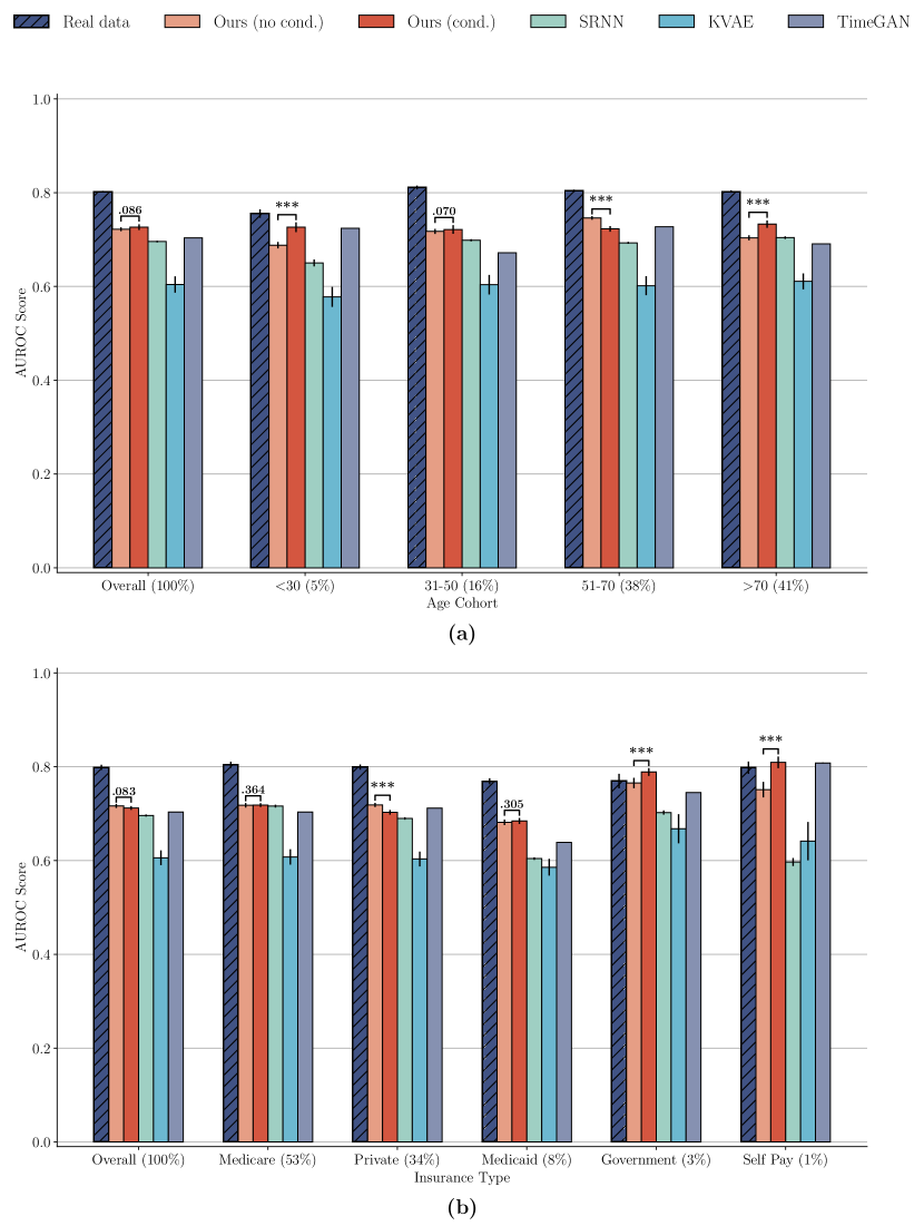
Figure A.1: Comparison of AUROC score between our model when conditionally and unconditionally generating synthetic data with baselines. We show these additional results of the vaso task for different age cohorts (a) as well for the range of insurance types (b). Significance levels between groups of interest are shown with brackets, where * corresponds to p $<$ 0.05, ** to p $<$ 0.01 and *** to p $<$ 0.001

Appendix B Implementation and Training Details

Here we provide additional details on the neural architectures of our model, and on the training hyperparameters for all models.

The approximate posterior distribution $q_{\phi_{\mathbf{v}}}(\mathbf{v}|\mathbf{x}_{1:T},\mathbf{m}_{1:T},\mathbf{s},\mathbf{y})$ of the static latent variable $\mathbf{v}$ is parameterized by a 2-layer Multilayer Perceptron (MLP), as shown in Table B.1. Both RNNs for $\mathbf{h}$ and $\mathbf{g}$ are implemented as GRU cells with an input size of 64 and hidden dimension 128. Their inputs are given by linear transformations of $[\mathbf{x}_{t},\mathbf{v}]$ and $[\mathbf{x}_{t},\mathbf{h}_{t},\mathbf{v}]$, respectively, followed by tanh. The dynamics models of the latent variable $\mathbf{z}_{t}$, both at inference and generation time, are implemented as 2-layer MLPs, presented in Table B.2. The generation of feature vectors $\mathbf{x}_{t}$ at each time step as well as the full sequence of missingness masks $\mathbf{m}_{1:T}$ are also implemented as MLPs, with details provided in Table B.3 and Table B.4, respectively.

We use the Adam optimization algorithm [28] to update the networks of all models presented in this work. The choices of hyperparameters for each model can be found in Table B.5. For the dynamical VAE baselines (SRNN and KVAE), we largely used the implementations provided by Girin et al. [18], with some slight changes and extensions. The implementation of our model, as well as the experimental pipeline necessary to reproduce our results, can be found at https://github.com/simonbing/HealthGen.

Our experiments were conducted on a high-performance compute cluster, consisting mainly of NVIDIA V100 GPUs. In order to reproduce our results on a comparable hardware architecture, it would take approximately 200 GPU days.

Table B.1: MLP encoder that parameterizes the approximate posterior distribution $q_{\phi_{\mathbf{v}}}(\mathbf{v}|\mathbf{x}_{1:T},\mathbf{m}_{1:T},\mathbf{s},\mathbf{y})$ of the static latent variable $\mathbf{v}$. The input is the concatenation of $[\mathbf{x}_{1:T},\mathbf{m}_{1:T},\mathbf{s},\mathbf{y}]$ and the output vector is the mean and log variance of the distribution.

Input size	Output size	Activation	Bias
5201	256	tanh	True
256	128	tanh	True
128	64	-	True

Table B.2: MLP network architecture to parameterize $q_{\phi_{\mathbf{z}}}(\mathbf{z}_{t}|\mathbf{z}_{t-1},\mathbf{g}_{t})$ and $p_{\theta_{\mathbf{z}}}(\mathbf{z}_{t}|\mathbf{z}_{t-1},\mathbf{h}_{t})$, i.e. the latent dynamics in the inference and generative model. The inputs are the concatenation of $[\mathbf{z}_{t-1},\mathbf{g}_{t}]$ for inference, and $[\mathbf{z}_{t-1},\mathbf{h}_{t}]$ for generation. The output vector is the mean and log variance of the distribution.

Input size	Output size	Activation	Bias
160	64	tanh	True
64	32	tanh	True
32	64	-	True

Table B.3: MLP decoder to parameterize the generative distribution of the features, $p_{\theta_{\mathbf{x}}}(\mathbf{x}_{t}|\mathbf{z}_{t},\mathbf{h}_{t},\mathbf{v},\mathbf{s},\mathbf{y})$. The input is the concatenation of $[\mathbf{z}_{t},\mathbf{h}_{t},\mathbf{v},\mathbf{s},\mathbf{y}]$, the output is the mean and log variance of the distribution.

Input size	Output size	Activation	Bias
193	256	tanh	True
256	208	-	True

Table B.4: MLP decoder for the generative distribution of the missingness masks, $p_{\theta_{\mathbf{m}}}(\mathbf{m}_{1:T}|\mathbf{v},\mathbf{s},\mathbf{y})$. The input vector is the concatenation of $[\mathbf{v},\mathbf{s},\mathbf{y}]$ and the output vector contains the mean $\mu_{t,d}$ of the Bernoulli distributions that $p_{\theta_{\mathbf{m}}}(\mathbf{m}_{1:T}|\mathbf{v},\mathbf{s},\mathbf{y})$ factorizes into.

Input size	Output size	Activation	Bias
33	128	tanh	True
128	256	tanh	True
256	2600	sigmoid	True

Table B.5: Hyperparameter choices for all of the considered models in this work. Hyperparameters were optimized by randomly sampling 20 different configurations for each model and then selecting the combination that yielded the highest AUROC score on the vent task.

Model	Hyperparameter	Range / Value
GRU-D	Learning rate $\alpha$	5e-4, 1e-4, 1e-3
	Decay step for learning rate t [epochs]	0, 20
	Dimension of hidden state $\mathbf{h}$	32, 64, 128
HealthGen	Learning rate $\alpha$	5e-4, 1e-3, 5e-3
	Batch size	32, 64, 128
	Tradeoff parameter $\beta$	0.5, 1.0, 5.0, 10.0
	Dimension of static latent variable $\mathbf{v}$	16, 32, 64
	Dimension of dynamic latent variable $\mathbf{z}$	16, 32, 64
SRNN	Learning rate $\alpha$	5e-4, 1e-3, 5e-3
	Batch size	32, 64, 128
	Decay step for learning rate t [epochs]	0, 20
	Dropout percentage $p_{\text{dropout}}$	0, 0.1, 0.2, 0.3
	Dimension of latent variable $\mathbf{z}$	8, 16, 32
KVAE	Learning rate $\alpha$	3e-6, 1e-5, 3e-5
	Batch size	32, 64, 128
	Decay step for learning rate t [epochs]	0, 20
	Total training epochs	40, 50, 60, 70
	VAE only training epochs	10, 20, 30
	Kalman filter + VAE training epochs	10, 20, 30
	Tradeoff parameter $\beta$	0.3, 0.5, 1.0
	Number of linear state-space models $K$	5, 10, 20
	Dimension of intermed. latent variable $\mathbf{a}$	16, 32
	Dimension of latent variable $\mathbf{z}$	8, 16
TimeGAN	Batch size	32, 64, 128
	Number of layers $N$	2, 3, 5
	Dimension of the latent variable $\mathbf{h}$	8, 16, 24, 32

Appendix C Data set characteristics

Table C.1: Descriptive statistics of the features included in the MIMIC-III data set. The Value column shows the median value of the respective variable with the 10th and 90th percentiles indicated in parantheses. The right-most column shows the percentage of missing values for each input feature.

Feature	Value	Miss. [%]
Alanine aminotransferase	31.00 (12.00, 216.95)	98.198
Albumin	3.30 (2.30, 4.20)	98.710
Albumin ascites	1.45 (0.78, 3.03)	99.995
Albumin pleural	2.00 (1.10, 2.60)	99.996
Albumin urine	13.20 (1.40, 161.19)	99.994
Alkaline phosphate	84.00 (48.00, 205.00)	98.244
Anion gap	14.00 (10.00, 20.00)	94.942
Asparate aminotransferase	41.00 (17.00, 321.50)	98.197
Basophils	0.30 (0.10, 0.85)	98.533
Bicarbonate	24.00 (18.00, 28.00)	94.260
Bilirubin	0.70 (0.30, 3.50)	98.214
Blood urea nitrogen	18.00 (9.00, 50.00)	94.213
CO2	23.00 (17.00, 28.00)	98.515
CO2 (ETCO2, PCO2, etc.)	25.00 (20.00, 29.67)	92.637
Calcium	8.40 (7.20, 9.40)	96.178
Calcium ionized	1.14 (1.01, 1.28)	95.743
Calcium urine	2.40 (0.40, 13.08)	99.994
Cardiac Index	2.49 (1.82, 3.69)	98.056
Cardiac Output Thermodilution	4.90 (3.35, 7.20)	98.299
Cardiac Output fick	5.54 (3.70, 9.05)	99.707
Central Venous Pressure	11.00 (5.00, 17.00)	91.292
Chloride	105.00 (98.00, 112.00)	92.977
Chloride urine	47.00 (14.00, 116.60)	99.902
Cholesterol	164.00 (110.80, 226.20)	99.796
Cholesterol HDL	45.00 (30.00, 66.70)	99.834
Cholesterol LDL	93.00 (47.00, 147.00)	99.843
Creatinine	0.90 (0.60, 2.40)	94.201
Creatinine ascites	1.10 (0.56, 6.76)	99.998
Creatinine body fluid	1.10 (0.94, 1.66)	99.999
Creatinine pleural	1.20 (0.60, 3.25)	99.999
Creatinine urine	78.00 (24.00, 186.00)	99.736
Diastolic blood pressure	60.00 (44.50, 80.00)	68.667
Eosinophils	2.00 (1.00, 6.00)	99.981
Fibrinogen	220.00 (131.00, 434.00)	98.713
Fraction inspired oxygen	0.50 (0.40, 1.00)	98.022
Fraction inspired oxygen Set	0.50 (0.40, 1.00)	97.423
Glascow coma scale total	14.00 (3.00, 15.00)	94.824
Glucose	136.25 (95.00, 226.00)	88.420
Heart Rate	84.00 (63.00, 109.00)	68.040
Height	170.09 (154.97, 182.94)	99.440
Hematocrit	31.90 (24.10, 40.80)	91.177
Hemoglobin	10.80 (8.10, 13.90)	91.924
Lactate	2.00 (1.00, 4.88)	96.639
Lactate dehydrogenase	260.00 (156.00, 757.00)	99.228
Lactate dehydrogenase pleural	172.00 (65.20, 1485.00)	99.991
Lactic acid	2.10 (1.00, 5.10)	98.029
Lymphocytes	11.00 (3.80, 28.10)	98.061
Lymphocytes ascites	18.00 (2.00, 57.60)	99.982
Lymphocytes atypical	2.00 (1.00, 5.00)	99.874
Lymphocytes atypical CSL	1.50 (1.00, 3.00)	99.998
Lymphocytes body fluid	18.00 (2.00, 68.20)	99.973
Lymphocytes percent	13.00 (4.00, 39.00)	99.993
Lymphocytes pleural	30.00 (3.00, 79.40)	99.991
Magnesium	1.90 (1.50, 2.40)	95.863
Mean blood pressure	78.00 (61.00, 99.50)	68.884
Mean corpuscular hemoglobin	30.50 (27.50, 33.20)	95.043
Mean corpuscular hemoglobin concentration	34.10 (31.90, 35.80)	95.040
Mean corpuscular volume	89.00 (82.00, 97.00)	95.043
Monocytes	4.00 (1.70, 7.10)	98.081
Monocytes CSL	20.00 (4.00, 54.00)	99.966
Neutrophils	81.20 (60.00, 91.70)	98.050
Oxygen saturation	98.67 (94.00, 100.00)	67.963
Partial pressure of carbon dioxide	41.00 (32.00, 52.00)	92.637
Partial pressure of oxygen	195.00 (88.00, 387.00)	97.213
Partial thromboplastin time	30.60 (23.50, 55.50)	94.662
Peak inspiratory pressure	23.00 (14.00, 32.00)	97.442
Phosphate	3.50 (2.20, 5.30)	96.903
Phosphorous	3.40 (2.20, 5.20)	97.871
Plateau Pressure	18.00 (14.00, 25.00)	98.226
Platelets	203.00 (104.00, 352.00)	93.685
Positive end-expiratory pressure	5.00 (5.00, 10.00)	99.095
Positive end-expiratory pressure Set	5.00 (5.00, 8.00)	96.835
Post Void Residual	163.26 (65.40, 382.75)	99.955
Potassium	4.20 (3.40, 5.22)	91.172
Potassium serum	4.10 (3.40, 5.00)	98.676
Prothrombin time INR	1.30 (1.00, 2.00)	94.650
Prothrombin time PT	14.20 (12.20, 19.36)	94.652
Pulmonary Artery Pressure mean	26.00 (17.00, 40.00)	98.976
Pulmonary Artery Pressure systolic	33.00 (23.00, 47.00)	93.292
Pulmonary Capillary Wedge Pressure	16.00 (8.00, 27.00)	99.902
Red blood cell count	3.70 (2.75, 4.72)	95.039
Red blood cell count CSF	16.50 (1.00, 2950.00)	99.966
Red blood cell count ascites	1050.00 (43.20, 13450.00)	99.982
Red blood cell count pleural	3000.00 (182.60, 103866.40)	99.991
Red blood cell count urine	5.00 (1.00, 80.70)	99.701
Respiratory rate	17.00 (11.00, 25.00)	67.945
Respiratory rate Set	14.00 (10.00, 20.00)	97.250
Sodium	138.00 (133.00, 143.00)	92.165
Systemic Vascular Resistance	1037.04 (646.09, 1652.88)	98.060
Systolic blood pressure	117.00 (92.67, 150.00)	68.656
Temperature	36.56 (35.56, 37.61)	88.330
Tidal Volume Observed	564.00 (424.00, 800.00)	96.496
Tidal Volume Set	550.00 (450.00, 700.00)	97.480
Tidal Volume Spontaneous	460.00 (0.00, 714.00)	99.135
Total Protein	5.90 (4.83, 7.27)	99.990
Total Protein Urine	57.50 (13.00, 388.40)	99.967
Troponin-I	1.70 (0.30, 21.00)	99.914
Troponin-T	0.07 (0.01, 1.42)	98.723
Venous PvO2	43.00 (29.00, 71.00)	99.974
Weight	77.80 (55.50, 108.08)	97.047
White blood cell count	11.10 (5.70, 20.00)	94.052
White blood cell count urine	4.00 (1.00, 40.90)	99.706
pH	7.37 (7.27, 7.46)	92.402
pH urine	5.50 (5.00, 7.00)	98.473

Table C.1: (continued)

Table C.2: Percentage of positive samples for the extracted labels.

Label	Positive Class
vent	12.02%
vaso	10.30%
colloid_bolus	0.95%
crystalloid_bolus	9.61%
niv	37.74%

Table C.3: Summary of the static variables for the extracted MIMIC-III patient cohort.

Static variable		Patients
Sex	Female	14,978 (43%)
	Male	19,494 (57%)
Ethnicity	Asian	842 (2%)
	Hispanic	1,137 (3%)
	Black	2,667 (8%)
	Other	5,183 (15%)
	White	24,643 (71%)
Age	$<$30	1,832 (5%)
	31-50	5,489 (16%)
	51-70	12,942 (38%)
	$>$70	14,209 (41%)
Insurance Type	Self Pay	477 (1%)
	Government	1,050 (3%)
	Medicaid	2,782 (8%)
	Private	11,846 (34%)
	Medicare	18,317 (53%)

Appendix D Samples of synthetically generated data

For the additional synthetic data visualization we preform a preselection of the generated patients based on lower than average missingness, in order to visualize samples where dense measurements over time are present and the dynamics are more evident . After this preselection, we randomly select three patients to visualize amongst them in Figures D.1, LABEL:, D.2, LABEL: and D.5. We also show two examples of randomly selected patients without this preselection in Figures D.3, LABEL: and D.4.

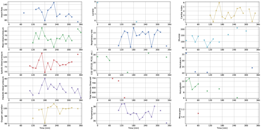
Figure D.1: Feature time series of a synthetically generated patient.

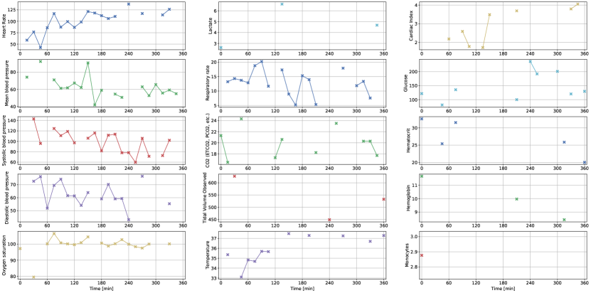
Figure D.2: Feature time series of a synthetically generated patient.

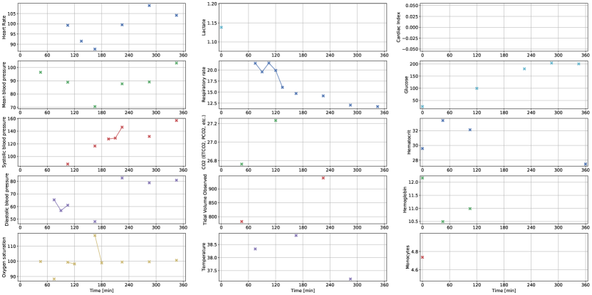
Figure D.3: Feature time series of a synthetically generated patient.

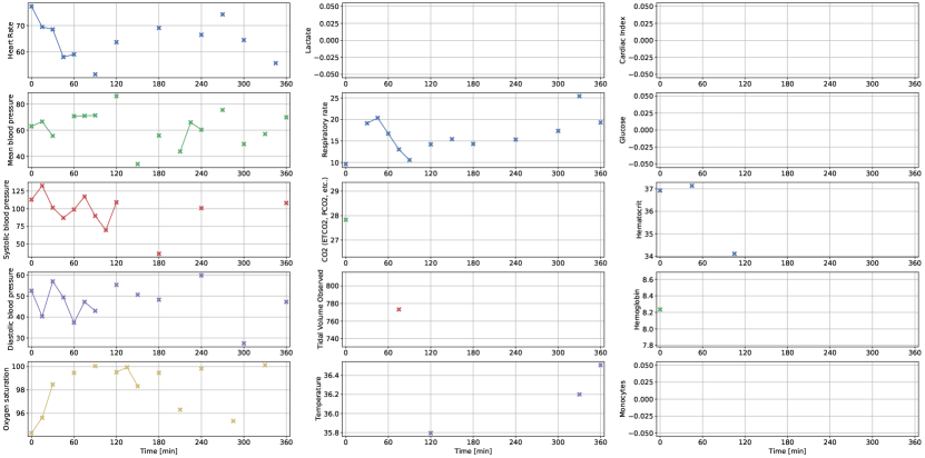
Figure D.4: Feature time series of a synthetically generated patient.

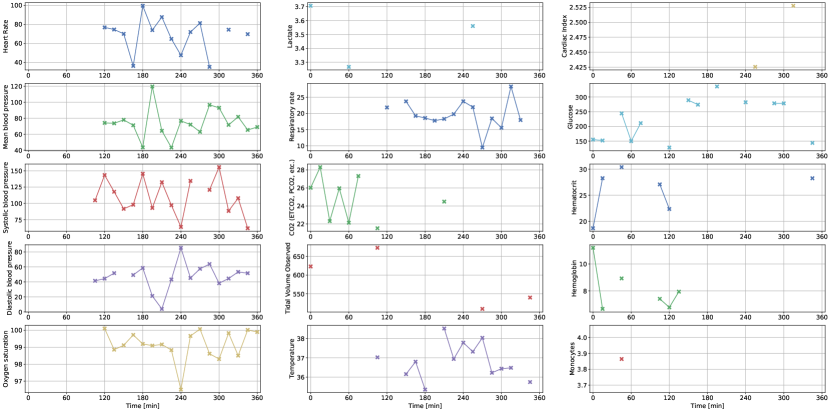
Figure D.5: Feature time series of a synthetically generated patient.-

References

- Ahmed et al. [2021] Ossama Ahmed, Frederik Träuble, Anirudh Goyal, Alexander Neitz, Manuel Wüthrich, Yoshua Bengio, Bernhard Schölkopf, and Stefan Bauer. Causalworld: A robotic manipulation benchmark for causal structure and transfer learning. In International Conference on Learning Representations, 2021.
- Alaa et al. [2021] Ahmed M. Alaa, Alex J. Chan, and Mihaela van der Schaar. Generative time-series modeling with fourier flows. In International Conference on Learning Representations, 2021.
- Buczak et al. [2010] Anna L. Buczak, Steven Babin, and Linda Moniz. Data-driven approach for creating synthetic electronic medical records. BMC Medical Informatics and Decision Making, 10(1):59, 2010.
- Che et al. [2018] Zhengping Che, Sanjay Purushotham, Kyunghyun Cho, David Sontag, and Yan Liu. Recurrent neural networks for multivariate time series with missing values. Scientific Reports, 8(1):6085, 2018.
- Chen et al. [2019] Junqiao Chen, David Chun, Milesh Patel, Epson Chiang, and Jesse James. The validity of synthetic clinical data: a validation study of a leading synthetic data generator (synthea) using clinical quality measures. BMC medical informatics and decision making, 19(1):1–9, 2019.
- Chen et al. [2021] Richard J Chen, Ming Y Lu, Tiffany Y Chen, Drew FK Williamson, and Faisal Mahmood. Synthetic data in machine learning for medicine and healthcare. Nature Biomedical Engineering, pages 1–5, 2021.
- Cho et al. [2014] Kyunghyun Cho, Bart van Merrienboer, Çaglar Gülçehre, Dzmitry Bahdanau, Fethi Bougares, Holger Schwenk, and Yoshua Bengio. Learning phrase representations using RNN encoder-decoder for statistical machine translation. In Proceedings of the 2014 Conference on Empirical Methods in Natural Language Processing, pages 1724–1734. ACL, 2014.
- Dash et al. [2020] Saloni Dash, Andrew Yale, Isabelle Guyon, and Kristin P Bennett. Medical time-series data generation using generative adversarial networks. In International Conference on Artificial Intelligence in Medicine, pages 382–391. Springer, 2020.
- Deng et al. [2009] Jia Deng, Wei Dong, Richard Socher, Li-Jia Li, Kai Li, and Li Fei-Fei. Imagenet: A large-scale hierarchical image database. In 2009 IEEE conference on computer vision and pattern recognition, pages 248–255, 2009.
- Dexter et al. [2020] Gregory Dexter, Shaun Grannis, Brian Dixon, and Suranga Nath Kasthurirathne. Generalization of machine learning approaches to identify notifiable conditions from a statewide health information exchange. AMIA Joint Summits on Translational Science proceedings, 2020:152–161, 2020.
- DuMont Schütte et al. [2021] August DuMont Schütte, Jürgen Hetzel, Sergios Gatidis, Tobias Hepp, Benedikt Dietz, Stefan Bauer, and Patrick Schwab. Overcoming barriers to data sharing with medical image generation: a comprehensive evaluation. npj Digital Medicine, 4(1):141, 2021.
- Dwork and Roth [2014] Cynthia Dwork and Aaron Roth. The algorithmic foundations of differential privacy. Foundations and Trends in Theoretical Computer Science, 9(3–4):211–407, 2014.
- Esteban et al. [2017] Cristóbal Esteban, Stephanie L. Hyland, and Gunnar Rätsch. Real-valued (medical) time series generation with recurrent conditional gans. arXiv preprint arXiv:1706.02633, 2017.
- Fraccaro et al. [2016] Marco Fraccaro, Søren Kaae Sønderby, Ulrich Paquet, and Ole Winther. Sequential neural models with stochastic layers. In Advances in Neural Information Processing Systems, 2016.
- Fraccaro et al. [2017] Marco Fraccaro, Simon Kamronn, Ulrich Paquet, and Ole Winther. A disentangled recognition and nonlinear dynamics model for unsupervised learning. In Advances in Neural Information Processing Systems, 2017.
- Frid-Adar et al. [2018] Maayan Frid-Adar, Eyal Klang, Michal Amitai, Jacob Goldberger, and Hayit Greenspan. Synthetic data augmentation using gan for improved liver lesion classification. In 2018 IEEE 15th international symposium on biomedical imaging (ISBI 2018), pages 289–293. IEEE, 2018.
- Ghassemi et al. [2015] Marzyeh Ghassemi, Marco Pimentel, Tristan Naumann, Thomas Brennan, David Clifton, Peter Szolovits, and Mengling Feng. A multivariate timeseries modeling approach to severity of illness assessment and forecasting in icu with sparse, heterogeneous clinical data. Proceedings of the AAAI Conference on Artificial Intelligence, 2015.
- Girin et al. [2020] Laurent Girin, Simon Leglaive, Xiaoyu Bie, Julien Diard, Thomas Hueber, and Xavier Alameda-Pineda. Dynamical variational autoencoders: A comprehensive review. arXiv preprint arXiv:2008.12595, 2020.
- Gohorbani et al. [2019] Amirata Gohorbani, Vivek Natarajan, David Devoud Coz, and Yuan Liu. Dermgan: Synthetic generation of clinical skin images with pathology. arXiv preprint arXiv:1911.08716, 2019.
- Goncalves et al. [2020] Andre Goncalves, Priyadip Ray, Braden Soper, Jennifer Stevens, Linda Coyle, and Ana Paula Sales. Generation and evaluation of synthetic patient data. BMC medical research methodology, 20(1):1–40, 2020.
- Goodfellow et al. [2014] Ian Goodfellow, Jean Pouget-Abadie, Mehdi Mirza, Bing Xu, David Warde-Farley, Sherjil Ozair, Aaron Courville, and Yoshua Bengio. Generative adversarial nets. In Advances in Neural Information Processing Systems, 2014.
- Henry et al. [2015] Katharine E. Henry, David N. Hager, Peter J. Pronovost, and Suchi Saria. A targeted real-time early warning score (trewscore) for septic shock. Science Translational Medicine, 7(299):299ra122, 2015.
- Hyland and Tople [2020] Stephanie L. Hyland and Shruti Tople. An empirical study on the intrinsic privacy of sgd. arXiv preprint arXiv:1912.02919, 2020.
- Hyland et al. [2020] Stephanie L. Hyland, Martin Faltys, Matthias Hüser, Xinrui Lyu, Thomas Gumbsch, Cristóbal Esteban, Christian Bock, Max Horn, Michael Moor, Bastian Rieck, Marc Zimmermann, Dean Bodenham, Karsten Borgwardt, Gunnar Rätsch, and Tobias M. Merz. Early prediction of circulatory failure in the intensive care unit using machine learning. Nature Medicine, 26(3):364–373, 2020.
- Jarrett et al. [2021] Daniel Jarrett, Ioana Bica, and Mihaela van der Schaar. Time-series generation by contrastive imitation. Advances in Neural Information Processing Systems, 34, 2021.
- Johnson et al. [2016] Alistair E. W. Johnson, Tom J. Pollard, Lu Shen, Li-wei H. Lehman, Mengling Feng, Mohammad Ghassemi, Benjamin Moody, Peter Szolovits, Leo Anthony Celi, and Roger G. Mark. Mimic-iii, a freely accessible critical care database. Scientific Data, 3(1):160035, 2016.
- Karras et al. [2019] Tero Karras, Samuli Laine, and Timo Aila. A style-based generator architecture for generative adversarial networks. In Proceedings of the IEEE/CVF Conference on Computer Vision and Pattern Recognition, pages 4401–4410, 2019.
- Kingma and Ba [2015] Diederik P. Kingma and Jimmy Ba. Adam: A method for stochastic optimization. In International Conference on Learning Representations, 2015.
- Kingma and Welling [2014] Diederik P. Kingma and Max Welling. Auto-encoding variational bayes. In International Conference on Learning Representations, 2014.
- Kohlberger et al. [2019] Timo Kohlberger, Yun Liu, Melissa Moran, Po-Hsuan Cameron Chen, Trissia Brown, Jason D. Hipp, Craig H. Mermel, and Martin C. Stumpe. Whole-slide image focus quality: Automatic assessment and impact on ai cancer detection. Journal of Pathology Informatics, 10:39, 2019.
- Ma and Zhang [2021] Chao Ma and Cheng Zhang. Identifiable generative models for missing not at random data imputation. In Advances in Neural Information Processing Systems, 2021.
- Mann and Whitney [1947] H. B. Mann and D. R. Whitney. On a Test of Whether one of Two Random Variables is Stochastically Larger than the Other. The Annals of Mathematical Statistics, 18(1):50 – 60, 1947.
- McDermott et al. [2018] Matthew McDermott, Tom Yan, Tristan Naumann, Nathan Hunt, Harini Suresh, Peter Szolovits, and Marzyeh Ghassemi. Semi-supervised biomedical translation with cycle wasserstein regression gans. Proceedings of the AAAI Conference on Artificial Intelligence, 2018.
- McSharry et al. [2003] P.E. McSharry, G.D. Clifford, L. Tarassenko, and L.A. Smith. A dynamical model for generating synthetic electrocardiogram signals. IEEE Transactions on Biomedical Engineering, 50(3):289–294, 2003.
- Nabi et al. [2020] Razieh Nabi, Rohit Bhattacharya, and Ilya Shpitser. Full law identification in graphical models of missing data: Completeness results. In International Conference on Machine Learning, pages 7153–7163, 2020.
- Pollard et al. [2018] Tom J. Pollard, Alistair E. W. Johnson, Jesse D. Raffa, Leo A. Celi, Roger G. Mark, and Omar Badawi. The eicu collaborative research database, a freely available multi-center database for critical care research. Scientific Data, 5(1):180178, 2018.
- Quiroz-Juárez et al. [2019] M. A. Quiroz-Juárez, O. Jiménez-Ramírez, R. Vázquez-Medina, V. Breña-Medina, J. L. Aragón, and R. A. Barrio. Generation of ecg signals from a reaction-diffusion model spatially discretized. Scientific Reports, 9(1):19000, 2019.
- Raghu et al. [2017] Aniruddh Raghu, Matthieu Komorowski, Leo Anthony Celi, Peter Szolovits, and Marzyeh Ghassemi. Continuous state-space models for optimal sepsis treatment: a deep reinforcement learning approach. In Proceedings of the 2nd Machine Learning for Healthcare Conference, pages 147–163, 2017.
- Razavian and Sontag [2015] Narges Razavian and David A. Sontag. Temporal convolutional neural networks for diagnosis from lab tests. arXiv preprint arXiv:1511.07938, 2015.
- Rieke et al. [2020] Nicola Rieke, Jonny Hancox, Wenqi Li, Fausto Milletarì, Holger R. Roth, Shadi Albarqouni, Spyridon Bakas, Mathieu N. Galtier, Bennett A. Landman, Klaus Maier-Hein, Sébastien Ourselin, Micah Sheller, Ronald M. Summers, Andrew Trask, Daguang Xu, Maximilian Baust, and M. Jorge Cardoso. The future of digital health with federated learning. npj Digital Medicine, 3(1):119, 2020.
- Rubin [1976] Donald B Rubin. Inference and missing data. Biometrika, 63(3):581–592, 1976.
- Sandfort et al. [2019] Veit Sandfort, Alistair E.W. Johnson, Lauren M. Kunz, Jose D. Vargas, and Douglas R. Rosing. Prolonged elevated heart rate and 90-day survival in acutely ill patients: Data from the mimic-iii database. Journal of Intensive Care Medicine, 34(8):622–629, 2019.
- Scheffer [2002] Judi Scheffer. Dealing with missing data. Research Letters in the Information and Mathematical Sciences, 3:153–160, 2002.
- Schwab et al. [2021] Patrick Schwab, Arash Mehrjou, Sonali Parbhoo, Leo Anthony Celi, Jürgen Hetzel, Markus Hofer, Bernhard Schölkopf, and Stefan Bauer. Real-time prediction of covid-19 related mortality using electronic health records. Nature Communications, 12(1):1058, 2021.
- Sheller et al. [2020] Micah J. Sheller, Brandon Edwards, G. Anthony Reina, Jason Martin, Sarthak Pati, Aikaterini Kotrotsou, Mikhail Milchenko, Weilin Xu, Daniel Marcus, Rivka R. Colen, and Spyridon Bakas. Federated learning in medicine: facilitating multi-institutional collaborations without sharing patient data. Scientific Reports, 10(1):12598, 2020.
- Skandarani et al. [2021] Youssef Skandarani, Pierre-Marc Jodoin, and Alain Lalande. Gans for medical image synthesis: An empirical study. arXiv preprin arXiv:2105.05318, 2021.
- Sohn et al. [2015] Kihyuk Sohn, Honglak Lee, and Xinchen Yan. Learning structured output representation using deep conditional generative models. In Advances in Neural Information Processing Systems, 2015.
- Suresh et al. [2017] Harini Suresh, Nathan Hunt, Alistair Johnson, Leo Anthony Celi, Peter Szolovits, and Marzyeh Ghassemi. Clinical intervention prediction and understanding using deep networks. arXiv preprint arXiv:1705.08498, 2017.
- Tomašev et al. [2019] Nenad Tomašev, Xavier Glorot, Jack W. Rae, Michal Zielinski, Harry Askham, Andre Saraiva, Anne Mottram, Clemens Meyer, Suman Ravuri, Ivan Protsyuk, Alistair Connell, Cían O. Hughes, Alan Karthikesalingam, Julien Cornebise, Hugh Montgomery, Geraint Rees, Chris Laing, Clifton R. Baker, Kelly Peterson, Ruth Reeves, Demis Hassabis, Dominic King, Mustafa Suleyman, Trevor Back, Christopher Nielson, Joseph R. Ledsam, and Shakir Mohamed. A clinically applicable approach to continuous prediction of future acute kidney injury. Nature, 572(7767):116–119, 2019.
- Tremblay et al. [2018a] Jonathan Tremblay, Aayush Prakash, David Acuna, Mark Brophy, Varun Jampani, Cem Anil, Thang To, Eric Cameracci, Shaad Boochoon, and Stan Birchfield. Training deep networks with synthetic data: Bridging the reality gap by domain randomization. In Proceedings of the IEEE conference on computer vision and pattern recognition workshops, pages 969–977, 2018a.
- Tremblay et al. [2018b] Jonathan Tremblay, Thang To, Balakumar Sundaralingam, Yu Xiang, Dieter Fox, and Stan Birchfield. Deep object pose estimation for semantic robotic grasping of household objects. In Conference on Robot Learning (CoRL), 2018b.
- Tucker et al. [2020] Allan Tucker, Zhenchen Wang, Ylenia Rotalinti, and Puja Myles. Generating high-fidelity synthetic patient data for assessing machine learning healthcare software. npj digital medicine, 3(1):1–13, 2020.
- Vahdat and Kautz [2020] Arash Vahdat and Jan Kautz. Nvae: A deep hierarchical variational autoencoder. In Advances in Neural Information Processing Systems, 2020.
- van Breugel et al. [2021] Boris van Breugel, Trent Kyono, Jeroen Berrevoets, and Mihaela van der Schaar. Decaf: Generating fair synthetic data using causally-aware generative networks. Advances in Neural Information Processing Systems, 34, 2021.
- van Panhuis et al. [2014] Willem G. van Panhuis, Proma Paul, Claudia Emerson, John Grefenstette, Richard Wilder, Abraham J. Herbst, David Heymann, and Donald S. Burke. A systematic review of barriers to data sharing in public health. BMC Public Health, 14(1):1144, 2014.
- Wang et al. [2020] Shirly Wang, Matthew B. A. McDermott, Geeticka Chauhan, Marzyeh Ghassemi, Michael C. Hughes, and Tristan Naumann. Mimic-extract: A data extraction, preprocessing, and representation pipeline for mimic-iii. In Proceedings of the ACM Conference on Health, Inference, and Learning, pages 222–235, 2020.
- Wood et al. [2021] Erroll Wood, Tadas Baltrušaitis, Charlie Hewitt, Sebastian Dziadzio, Matthew Johnson, Virginia Estellers, Thomas J. Cashman, and Jamie Shotton. Fake it till you make it: Face analysis in the wild using synthetic data alone. arXiv preprint arXiv:2109.15102, 2021.
- Yingzhen and Mandt [2018] Li Yingzhen and Stephan Mandt. Disentangled sequential autoencoder. In International Conference on Machine Learning, pages 5670–5679, 2018.
- Yoon et al. [2019] Jinsung Yoon, Daniel Jarrett, and Mihaela van der Schaar. Time-series generative adversarial networks. In Advances in Neural Information Processing Systems, 2019.
- Zech et al. [2018] John R. Zech, Marcus A. Badgeley, Manway Liu, Anthony B. Costa, Joseph J. Titano, and Eric Karl Oermann. Variable generalization performance of a deep learning model to detect pneumonia in chest radiographs: A cross-sectional study. PLOS Medicine, 15(11):1–17, 2018.