Multifractal behaviour in multiparticle production in $pp$ collisions at $\sqrt{s}=$ 0.9, 7 and 8 TeV from the CMS experiment

Abstract

Multifractal analysis was performed on $pp$ collision data at $\sqrt{s}=$ 0.9, 7 and 8 TeV from the CMS experiment at CERN. The data was obtained and processed from the CERN Open Data Portal. Vertical analysis was used to compute the generalised dimensions $D_{q}$ and the multifractal spectra $f(\alpha)$ of the data, which reveals the level of complexity of its pseudorapidity distribution. It was found that the $f(\alpha)$ curves widen with increasing collision energy, signalling an increase in branching complexity.

1 Multifractal formalism for multiparticle production

Multifractal analysis is a powerful tool used to characterise the complexity of data. It is highly multi-disciplinary in nature, finding applications in the analysis of a wide variety of complex systems, such as studying tectonic processes [1], medical signal analysis [2] and time series analysis in meteorology [3]. Here, we re-introduce a formalism tailored for investigating multiparticle production, as formulated by Hwa [4]. As with the original formulations, rapidity $y$ will be used in the presentation, but will be substituted with pseudorapidity $\eta$ when processing the data.

G-moments

Multifractal analysis in the context of multiparticle production was originally done by computing the G-moments of multiplicity distributions [4, 5, 6]. We begin by considering a single rapidity interval $\delta y$ and a collection of $N$ events. Each event $i$ has multiplicity $n_{i}$, and $K=\sum_{i=1}^{N}n_{i}$ is the total number of particles in $\delta y$ summed over all events.

The G-moment for the collection of $N$ events in $\delta y$ is then defined as

$$G_{q}(\delta y)={\sum_{i=1}^{N}}{{}^{\prime}p_{i}}^{q},$$ (1)

where $p_{i}=\frac{n_{i}}{K}$ is the probability of finding a particle in the $i$^th event. The prime indicates $G_{q}$ is summed only over non-empty events (i.e. all $p_{i}>0$), so we can have $q\in\mathbb{R}$. However, $G_{q}(\delta y)$ is very sensitive to statistical fluctuations for small $N$, and modified definitions have been proposed in [7].

The quantity being summed over ($p_{i}$ in our case) is called a measure. $q$ acts as a probing parameter – higher values would enhance the differences between the $p_{i}$’s. Changing $\delta y$ explores the phase space at different scales. As such, $G_{q}(\delta y)$ is sometimes called the partition function in multifractal analysis [1] as it encodes information at different scales $\delta y$ and at different moments $q$. This scheme of setting up $G_{q}(\delta y)$ is analogous to the box counting algorithm commonly used in digital image analysis.

Properties of $G_{q}(\delta y)$

Suppose that for some event $i$, its $p_{i}$ value scales as

$$p_{i}\propto(\delta y)^{\alpha_{i}}$$ (2)

for some exponent $\alpha_{i}$. For a multifractal system, the $\alpha_{i}$’s are generally different and can take on a range of values, reflecting different subsets of the data with local scaling behaviour. Let $S_{\alpha^{\prime}}$ be a set containing all the events that scale according to equation 2, with the same value of $\alpha^{\prime}$. Furthermore, let $N_{\alpha^{\prime}}(\delta y)$ denote the cardinality of $S_{\alpha^{\prime}}$. Multifractals generally have the property that [4, 1]

$$N_{\alpha^{\prime}}(\delta y)\propto(\delta y)^{-f(\alpha^{\prime})},$$ (3)

i.e. the collection of events that scale according to equation 2 with a particular value of $\alpha^{\prime}$ in a particular window $\left[\alpha^{\prime},\alpha^{\prime}+d\alpha^{\prime}\right]$ form a fractal subset (of a larger set of more fractal subsets corresponding to other values of $\alpha$), and its cardinality scales with fractal dimension $f(\alpha^{\prime})$. It is in this sense that the union of fractal subsets form a multifractal.

$N_{\alpha^{\prime}}(\delta y)$ has been suggested by Halsey et al. [8] to be of the form [4]

$$N_{\alpha^{\prime}}(\delta y)=\int_{\alpha^{\prime}}^{\alpha^{\prime}+d\alpha^{\prime}}d\alpha h(\alpha)(\delta y)^{-f(\alpha)},$$ (4)

for some continuous function $h(\alpha)$. With equation 4, we can now re-express $G_{q}(\delta y)$ as

$$\begin{split}G_{q}(\delta y)&={\sum_{m=1}^{M}}{{}^{\prime}p_{m}}^{q}\\ &\propto{\sum_{m=1}^{M}}{{}^{\prime}(\delta y)}^{q\alpha_{m}}\\ &=\int d\alpha h(\alpha)(\delta y)^{-f(\alpha)}(\delta y)^{q\alpha}\\ &=\int d\alpha h(\alpha)(\delta y)^{q\alpha-f(\alpha)}.\end{split}$$ (5)

The resulting dependence of $G_{q}(\delta y)$ on $\delta y$ can be expressed as [4]

$$G_{q}(\delta y)\propto(\delta y)^{\tau(q)},$$ (6)

where $\tau(q)$ has been established by Hentschel and Procaccia [9] to be

$$\tau(q)=(q-1)D_{q}.$$ (7)

$D_{q}$ is known as the generalised dimension of order $q$, which can be experimentally obtained by rearranging equation 7:

$$D_{q}=\lim\limits_{\delta y\rightarrow 0}\left[\frac{1}{q-1}\frac{\ln G_{q}(\delta y)}{\ln(\delta y)}\right].$$ (8)

It must be noted that in experimental measurements, the mathematical limit $\delta y\rightarrow 0$ in equation 8 cannot be realised. The finiteness of particle multiplicity produced from finite energy implies that self-similar and fractal structures, if present, cannot persist indefinitely to finer scales of resolution [10]. Additionally, the detector resolution also imposes a lower limit on the probing scale.

The goal in multifractal analysis is to study the dependence of $G_{q}(\delta y)$ on $\delta y$, and the $D_{q}$’s are the main quantities that summarise the relation. $D_{0}$, $D_{1}$ and $D_{2}$ are also known as the fractal, information and correlation dimensions respectively [9, 4]. A monofractal has constant $D_{q}$ for all $q$; otherwise, it is a multifractal [1].

The above approach using the G-moments does not assume any specific dynamical model of multiparticle production [10], which serves as a model-agnostic tool to describe the complexity within data.

2 Vertical and horizontal averaging

By construction, the G-moment described in the previous section accesses a very small subset of the data – only one rapidity interval over all $N$ events. The G-moments computed this way is also known as the vertical moments [4], notated as $G_{q}^{\text{(v)}}$.

Alternatively, one can also analyse all the rapidity intervals in a single event. The G-moments computed this way is known as the horizontal moments [4], notated as $G_{q}^{\text{(h)}}$.

Since both methods access only a small slice of the available data, the statistics can be enhanced by supplementing the vertical moments with horizontal averaging, and vice versa. For example, the vertical moments can be calculated for every $\delta y$ interval and averaged horizontally over the $M$ bins:

$$\left<G_{q}^{\text{(v)}}\right>\equiv\frac{1}{M}\sum_{m}^{M}G_{q}^{\text{(v)}}.$$ (9)

Likewise, the horizontal moments can be calculated for every event and averaged vertically over all $N$ events:

$$\left<G_{q}^{\text{(h)}}\right>\equiv\frac{1}{N}\sum_{i}^{N}G_{q}^{\text{(h)}}.$$ (10)

In general, we have $\left<G_{q}^{\text{(v)}}\right>\neq\left<G_{q}^{\text{(h)}}\right>$ except when $q=1$. The two moments also capture different features of the dataset; for example, $\left<G_{q}^{\text{(v)}}\right>$ would be sensitive to rare events with very high multiplicity, while $\left<G_{q}^{\text{(h)}}\right>$ would not. $\left<G_{q}^{\text{(h)}}\right>$ however, describes a more intuitive notion of fractal structures within the multiparticle production in each event. Florkowski and Hwa [10] have studied the limiting scenarios in which they are equivalent, under the assumptions of ergodicity.

Contemporary multiplicity measurements (e.g. [11]) are statistically derived quantities, with $P(n)$ interpreted as an average over many events that has undergone an unfolding process. The pseudorapidity distribution of single events is not available as a result. Hence, we will perform our multifractal analysis using the vertical moments with horizontal averaging (equation 9).

3 The $f(\alpha)$ spectrum

As multifractals cannot be described by a single fractal dimension, a singularity spectrum or Legendre spectrum, $f(\alpha)$ is used to characterise them instead, which encodes the spread of $\alpha$ values exhibited by the system.

To obtain the $f(\alpha)$ spectrum, consider again equation 5:

$$G_{q}(\delta y)=\int d\alpha h(\alpha)(\delta y)^{q\alpha-f(\alpha)}.$$

Suppose $h(\alpha)\neq 0$. For each value of $q$ and in the limit $\delta y\rightarrow 0$, the integral would have most of its contribution from some value $\alpha$ which makes the exponent $q\alpha-f(\alpha)$ smallest. Let this optimising value of $\alpha$ be $\alpha_{q}$. To minimise the exponent, we require

$$\left.\frac{d}{d\alpha}\left[q\alpha-f(\alpha)\right]\right|_{\alpha=\alpha_{q}}=0,$$ (11)

$$\left.\frac{d^{2}}{d\alpha^{2}}\left[q\alpha-f(\alpha)\right]\right|_{\alpha=\alpha_{q}}>0,$$ (12)

which result in

$$f^{\prime}(\alpha_{q})=q,$$ (13)

$$f^{\prime\prime}(\alpha_{q})<0.$$ (14)

Substituting equations 13 and 14 into 8, and using the saddle point approximation, we get

$$\begin{split}D_{q}&=\lim\limits_{\delta y\rightarrow 0}\left[\frac{1}{q-1}\frac{\ln G_{q}(\delta y)}{\ln(\delta y)}\right]\\ &=\lim\limits_{\delta y\rightarrow 0}\left[\frac{1}{q-1}\frac{\ln\int d\alpha h(\alpha)(\delta y)^{q\alpha-f(\alpha)}}{\ln(\delta y)}\right]\\ &\approx\lim\limits_{\delta y\rightarrow 0}\left[\frac{1}{q-1}\frac{\ln\left[d\alpha h(\alpha_{q})(\delta y)^{q\alpha_{q}-f(\alpha_{q})}\right]}{\ln(\delta y)}\right]\\ &=\lim\limits_{\delta y\rightarrow 0}\left[\frac{1}{q-1}\frac{\ln\left[d\alpha h(\alpha_{q})\right]+\ln(\delta y)^{q\alpha_{q}-f(\alpha_{q})}}{\ln(\delta y)}\right]\\ \therefore D_{q}&\approx\frac{q\alpha_{q}-f(\alpha_{q})}{q-1}=\frac{\tau(q)}{q-1}.\end{split}$$ (15)

Equation 15 reveals how all the quantities in multifractal analysis relate to each other and how they can be computed. First, $\tau(q)$ can be evaluated by [4]

$$\tau(q)=\lim\limits_{\delta y\rightarrow 0}\left[\frac{\ln G_{q}(\delta y)}{\ln(\delta y)}\right],$$ (16)

which also gives $D_{q}$ via equation 8. In our analysis, $G_{q}(\delta y)$ will be replaced by $\left<G_{q}^{\text{(v)}}\right>$ (equation 9).

Next, $\alpha_{q}$ is obtained via numerical differentiation [4]:

$$\alpha_{q}=\frac{d}{dq}\tau(q).$$ (17)

This finally allows us to compute $f(\alpha)$ [4]:

$$f(\alpha_{q})=q\alpha_{q}-\tau(q).$$ (18)

For a multifractal, equations 13 and 14 indicate that the curve $f(\alpha)$ has a maximum at $\alpha_{0}$ and is concave downward everywhere. In the case of a monofractal, only a single value of $\alpha$ exists and the $f(\alpha)$ spectrum would reduce to a point [1].

What does the $f(\alpha)$ curve tell us?

In general, $f(\alpha)$ curves in multifractal analysis describes the complexity of a signal [1]. In the context of our analysis, it describes the smoothness (or roughness) of the pseudorapidity distribution of our multiplicity data, $N(\eta)$. A low value of $\alpha_{0}$ indicates a smoother $N(\eta)$. The width $W$ reflects the range of fractal exponents embedded in the dataset – larger values of $W$ reflect a more complex $N(\eta)$ distribution (i.e. greater degree of multifractality).

4 About the data

This analysis is performed on Run 1 data from the CMS collaboration processed from the CMS Open Data Portal, covering centre-of-mass energies $\sqrt{s}=$ 0.9, 7 and 8 TeV. The analysis method follows largely that of CMS [11], which analysed minimum-bias (MinBias), non-single diffractive (NSD) multiplicity distributions.

NSD events were selected by requiring that at least one forward hadron (HF) calorimeter tower on each side of the detector have at least 3 GeV of energy deposited in the event. The primary vertex was chosen as the vertex with the highest number of associated tracks, which must also be within 15 cm of the reconstructed beamspot in the beam axis and be of good reconstruction quality (ndof $>$ 4).

Good quality tracks were selected by requiring them to carry the highPurity label. Furthermore, we select for tracks with $<$10% relative error on the transverse momentum ($p_{\text{T}}$) measurement ($\sigma_{p_{\text{T}}}/p_{\text{T}}<0.1$) to reject low-quality and badly reconstructed tracks. Secondaries were removed by requiring a small impact parameter with respect to the selected primary vertex. Also, tracks were required to have $p_{\text{T}}>500$ MeV/c, which will be extrapolated to zero via unfolding.

Finally, unfolding was performed using an iterative “Bayesian unfolding method”, which is more accurately known as “D’Agostini iteration with early stopping” and described in [12]. This infers the original charged hadron multiplicity distribution (MinBias NSD) from the charged track multiplicity distribution measured.

Tables 2 and 3 in the Appendix summarise the datasets used.

5 Results and Discussion

Table 1 summarises the results of our multifractal analysis, giving the generalised dimensions $D_{q}$ and an approximate description of the width of the $f(\alpha)$ curves.

Table 1: Generalised dimensions and width of $f(\alpha)$ curves from multifractal analysis of $pp$ collisions at $\sqrt{s}=$ 0.9, 7 and 8 TeV, with all values normalised to $D_{0}$ at $\sqrt{s}=$ 900 GeV. $\alpha_{\text{max}}$ and $\alpha_{\text{min}}$ are evaluated at $q=-20$ and $q=+20$ respectively.

$\sqrt{s}$	900 GeV	7 TeV	8 TeV
$D_{0}$	1	0.996	0.996
$D_{1}$	0.988	0.980	0.978
$D_{2}$	0.975	0.965	0.961
$D_{3}$	0.964	0.952	0.948
$D_{4}$	0.954	0.941	0.937
$D_{5}$	0.946	0.932	0.927
$\alpha_{\text{min}}$	0.838	0.829	0.826
$\alpha_{\text{max}}$	1.054	1.068	1.072
$W$	0.216	0.239	0.246

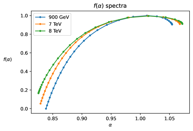
Figure 1: $f(\alpha)$ spectra of $pp$ collisions at $\sqrt{s}=$ 0.9, 7 and 8 TeV.

Mathematically, the data points that constitute the $f(\alpha)$ curves are plotted by evaluating equation 18 for $q\in\mathbb{R}$. However, this is computationally impossible, as equation 1 would produce infinities for $q\rightarrow-\infty$ and infinitesimally small values for $q\rightarrow+\infty$; both scenarios would lead to numerical instabilities. Since the goal is to obtain a relative comparsion of the widths of the $f(\alpha)$ curves, we restricted the computation of data points to $-20\leq q\leq 20$. The distance between these data points at these limiting values of $q$ in the $\alpha$-axis would be our estimate of the $f(\alpha)$ width, $W$.

Figure 1 shows that the $f(\alpha)$ curves clearly broaden with increasing collision energy (which is also detailed in Table 1). This is a reflection of increasing complexity in the multiplicity data.

6 Conclusion

The techniques in multifractal analysis provide a model-independent means of describing the inherent complexity within the structures of the multiplicity distribution. We have used it to analyse $pp$ collisions at $\sqrt{s}=$ 0.9, 7 and 8 TeV and found that the $f(\alpha)$ curves broaden with increasing collision energy. This reflects an increase in complexity of the pseudorapidity distribution of the data. At higher energies, we would expect the $f(\alpha)$ curves to broaden further.

Appendix A Datasets used

Table 2: Summary of CMS collider datasets used from CERN Open Data Portal

$\sqrt{s}$	Dataset	Ref.
(TeV)
0.9	/MinimumBias/Commissioning10-07JunReReco_900GeV/RECO	[13]
7	/MinimumBias/Run2010A-Apr21ReReco-v1/AOD	[14]
8	/MinimumBias/Run2012B-22Jan2013-v1/AOD	[15]

Table 3: Summary of Monte Carlo datasets used from CERN Open Data Portal

$\sqrt{s}$	Dataset	Ref.
(TeV)
0.9	/MinBias_TuneZ2_900GeV_pythia6_cff_py	[16]
	_GEN_SIM_START311_V2_Dec11_v2
7	/MinBias_TuneZ2star_7TeV_pythia6/Summer12-LowPU2010	[17]
	_DR42-PU_S0_START42_V17B-v1/AODSIM
8	/MinBias_TuneZ2star_8TeV-pythia6/Summer12_DR53X-PU	[18]
	_S10_START53_V7A-v1/AODSIM

References

- [1] Luciano Telesca, Gerardo Colangelo, Vincenzo Lapenna and Maria Macchiato “Monofractal and multifractal characterization of geoelectrical signals measured in southern Italy” In Chaos, Solitons & Fractals 18.2, 2003, pp. 385–399 DOI: https://doi.org/10.1016/S0960-0779(02)00655-0
- [2] R. Lopes and N. Betrouni “Fractal and multifractal analysis: A review” In Medical Image Analysis 13.4, 2009, pp. 634–649 DOI: 10.1016/j.media.2009.05.003
- [3] Jaromir Krzyszczak et al. “Multifractal characterization and comparison of meteorological time series from two climatic zones” In Theoretical and Applied Climatology 137, 2019 DOI: 10.1007/s00704-018-2705-0
- [4] Rudolph C. Hwa “Fractal Measures in Multiparticle Production” In Phys. Rev. D 41, 1990, pp. 1456 DOI: 10.1103/PhysRevD.41.1456
- [5] L. K. Chen, A. H. Chan and C. K. Chew “Multifractality and high-energy multiparticle production” In Z. Phys. C 60, 1993, pp. 503–507 DOI: 10.1007/BF01560048
- [6] E. A. De Wolf, I. M. Dremin and W. Kittel “Scaling laws for density correlations and fluctuations in multiparticle dynamics” In Phys. Rept. 270, 1996, pp. 1–141 DOI: 10.1016/0370-1573(95)00069-0
- [7] Rudolph C. Hwa and Ji-cai Pan “Fractal behavior of multiplicity fluctuations in high-energy collisions” In Phys. Rev. D 45, 1992, pp. 1476–1483 DOI: 10.1103/PhysRevD.45.1476
- [8] Thomas C. Halsey et al. “Fractal measures and their singularities: The characterization of strange sets” [Erratum: Phys.Rev.A 34, 1601 (1986)] In Phys. Rev. A 33, 1986, pp. 1141–1151 DOI: 10.1103/PhysRevA.33.1141
- [9] H. G. E. Hentschel and Itamar Procaccia “The infinite number of generalized dimensions of fractals and strange attractors” In Physica 8, 1983, pp. 435–444 DOI: 10.1016/0167-2789(83)90235-X
- [10] Wojciech Florkowski and Rudolph C. Hwa “Universal multifractality in multiparticle production” In Phys. Rev. D 43, 1991, pp. 1548–1554 DOI: 10.1103/PhysRevD.43.1548
- [11] Vardan Khachatryan “Charged Particle Multiplicities in Interactions at , 2.36, and 7 TeV” In JHEP 01, 2011, pp. 079 DOI: 10.1007/JHEP01(2011)079
- [12] G. D’Agostini “A Multidimensional unfolding method based on Bayes’ theorem” In Nucl. Instrum. Meth. A 362, 1995, pp. 487–498 DOI: 10.1016/0168-9002(95)00274-X
-
[13]
CMS collaboration (2019)
“MinimumBias primary dataset in RECO format from the 0.9 TeV
Commissioning run of 2010
(/MinimumBias/Commissioning10-07JunReReco_900GeV/RECO). CERN Open Data
Portal.
DOI:10.7483/OPENDATA.CMS.1R58.OMBD” -
[14]
CMS collaboration (2019)
“MinimumBias primary dataset in AOD format from RunA of 2010
(/MinimumBias/Run2010A-Apr21ReReco-v1/AOD). CERN Open Data Portal.
DOI:10.7483/OPENDATA.CMS.6B3H.TR6Z” -
[15]
CMS collaboration (2017)
“MinimumBias primary dataset in AOD format from RunB of 2012
(/MinimumBias/Run2012B-22Jan2013-v1/AOD). CERN Open Data Portal.
DOI:10.7483/OPENDATA.CMS.HU6U.DRLD” -
[16]
CMS Collaboration (2019)
“Simulated dataset
MinBias_TuneZ2_900GeV_pythia6_cff_py_GEN_SIM_
START311_V2_Dec11_v2 in GEN-SIM-RECO format for 2010 commissioning data. CERN Open Data Portal.
DOI:10.7483/OPENDATA.CMS.JPB5.X7CN” -
[17]
CMS Collaboration (2018)
“Simulated dataset MinBias_TuneZ2star_7TeV_pythia6 in
AODSIM format for 2010 collision data. CERN Open Data Portal.
DOI:10.7483/OPENDATA.CMS.VTJ2.E5JN” -
[18]
CMS Collaboration (2021)
“Simulated dataset MinBias_TuneZ2star_8TeV-pythia6 in
AODSIM format for 2012 collision data. CERN Open Data Portal.
DOI:10.7483/OPENDATA.3GIM.7SPW”