Fine-Grained Trajectory-based Travel Time Estimation for Multi-city Scenarios Based on
Deep Meta-Learning

Abstract

Travel Time Estimation (TTE) is indispensable in intelligent transportation system (ITS). It is significant to achieve the fine-grained Trajectory-based Travel Time Estimation (TTTE) for multi-city scenarios, namely to accurately estimate travel time of the given trajectory for multiple city scenarios. However, it faces great challenges due to complex factors including dynamic temporal dependencies and fine-grained spatial dependencies. To tackle these challenges, we propose a meta learning based framework, MetaTTE, to continuously provide accurate travel time estimation over time by leveraging well-designed deep neural network model called DED, which consists of Data preprocessing module and Encoder-Decoder network module. By introducing meta learning techniques, the generalization ability of MetaTTE is enhanced using small amount of examples, which opens up new opportunities to increase the potential of achieving consistent performance on TTTE when traffic conditions and road networks change over time in the future. The DED model adopts an encoder-decoder network to capture fine-grained spatial and temporal representations. Extensive experiments on two real-world datasets are conducted to confirm that our MetaTTE outperforms six state-of-art baselines, and improve 29.35% and 25.93% accuracy than the best baseline on Chengdu and Porto datasets, respectively.

I Introduction

Travel time estimation (TTE) plays a vital role in mobile navigation [1], route planning [2] and ride-hailing services [3, 4]. It is reported that, Baidu Maps, which is one of the largest mobile map applications, has over 340 million monthly active users worldwide by the end of December 2016  [5]. In order to estimate travel time for users who desires to know the traffic condition in advance and wisely plan their upcoming trips, it is significant to develop a TTE model which is able to provide accurate travel time estimation over time in real applications.

In this paper, we focus on the fine-grained end-to-end Trajectory-based Travel Time Estimation (TTTE) for multi-city scenarios. Given historical trajectory data in multiple cities, our objective is to train single model and provide accurate travel time estimation over time for all city scenarios. Please note that it is different from other end-to-end trajectory-based methods, which either heavily rely on road networks of specific cities  [6, 3, 7, 8, 4, 5, 9] or require careful preprocessing for historical trajectories of specific cities [10, 11, 12].

However, it faces great challenges to provide accurate travel time estimation in real applications over time, as the TTTE is affected by many complex factors:

• Dynamic temporal dependencies. Travel time estimation is influenced by complex temporal factors, including the time varying traffic conditions and evolving road networks. On one hand, traffic conditions which implicitly influence travel time estimation change over time (i.e. peak and off-peak hours in a day, different days in a week etc.). On the other hand, road networks that impacts the travel time are varying when roadworks are undertaken, or streets are temporarily closed due to emergencies or regional restrictions etc., which frequently happens in large cities. Some TTTE studies  [6, 3, 7, 8, 4, 5, 9] utilize road network and traffic condition information in different cities and provide travel time estimations with different models, which performs well on their datasets. However, since the traffic conditions and road networks dynamically change over time, travel time estimation model is required to quickly fit latest traffic data to achieve satisfied performance consistently. The aforementioned methods heavily rely on large amount of historical traffic data which limits these models to continuously provide accurate estimation in a fast learning scheme.

• Fine-grained spatial dependencies. Some TTTE studies  [10, 11, 12] carefully preprocess trajectories when providing travel time estimation using raw trajectory data. DeepTTE  [10], for instance, resamples each trajectory data such that the distance gap between two consecutive points are relatively within the same range (i.e. 200 to 400 meters). However, the fine-grained spatial dependencies in daily scenarios whose distance gap ranges are less than 200 meters or more than 400 meters are ignored. As illustrated in Figure 1, we assume that there are two users using route planning applications to navigate themselves to the destination, with the route $A\rightarrow B$ and route $C\rightarrow D$, respectively. For route $A\rightarrow B$, there are many crossings in the whole trajectory which may contains several key GPS points (at the crossing) with 50 to 100-meter distance gap between neighboring points. The area masked with smaller red circle contains short-term features (i.e. the travel speed of the vehicles is slower and the traffic condition is relatively bad) of the road segments with less than 200-meter distance gaps which cannot be captured by DeepTTE For route $C\rightarrow D$, the whole trajectory may contain some key GPS points (at the crossing) with long distance gaps on express way which may exceeds 2 kilometers. The area masked with larger grey circle contains long-distance features (i.e. the travel speed of the vehicles is faster and the traffic condition is relatively good) corresponding to the road segments with more than 400-meter distance gaps, which cannot also be captured by DeepTTE either.

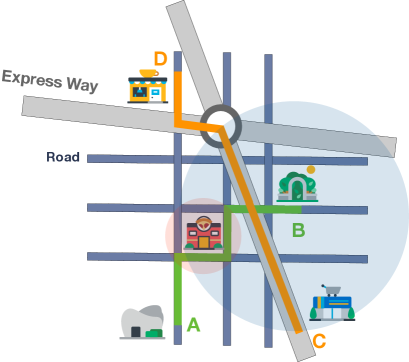
Figure 1: Two types of common scenarios in route planning applications. Route $A\rightarrow B$ contains relatively short distance gaps between adjacent key GPS points, while route $C\rightarrow D$ contains long distance gaps between adjacent key GPS points.

Therefore, it’s necessary to design a novel fine-grained model to simultaneously capture the dynamic temporal dependencies and fine-grained spatial dependencies, which is able to continuously provide accurate travel time estimation over time. Most existing works which utilizing conventional deep learning techniques ignore the fine-grained spatial dependencies and is limited to provide accurate travel time estimation in specific city at current time period as mentioned before.

To the best of our knowledge, this is the first work that investigates the potential of the fine-grained TTTE to continuously provide accurate travel time estimations for multi-city scenarios over time in a fast learning manner based on meta learning. To address the above challenges, we mainly make the following contributions:

• We construct two TTE-Tasks from two real-world datasets for training, corresponding to Chengdu, China and Porto, Portugal and divide the whole dataset into different sub-datasets which contains regional trajectories. Since every trajectory data is restricted to one unique region, MetaTTE is capable of quickly fitting latest trajectory data by simply adding a task using single model instead of training multiple models for multi-city scenarios which limits the ability of fast learning.

• We propose a novel deep neural network model called DED in the meta learning based framework (MetaTTE), which consists of two modules: (i) Data preprocessing module to remove the biases of outliers in real-world datasets and transform data into proper forms; (ii) Encoder-Decoder network module to firstly embed the spatial and temporal attributes into spatial, short-term and long-term embeddings, capture fine-grained spatial dependencies using recurrent neural network (RNN), fuse high level features using attention mechanism and finally estimate the travel time for multi-city scenarios.

• Moreover, to tackle the dynamic temporal dependencies, we introduce meta learning techniques into travel time estimation, which opens up new opportunities to continuously provide accurate travel time estimations over time, especially to increase the potential of achieving consistent performance when traffic conditions and road networks change over time in the future.

• By introducing meta-learning techniques, we enhance the generalization ability of MetaTTE using small amount of data from different TTE-Tasks. This enables our model to learn to learn, which increases the potential of accurate estimation in the future and decreases the time consumption to achieve the goal of fast learning.

• We conduct extensive experiments on two real-world large scale datasets collected in Chengdu, China and Porto, Portugal. The evaluation results show that our MetaTTE outperforms other state-of-art baselines. The source codes of MetaTTE are publicly available at Github.

The remaining of this paper is organized as follows: Section II introduces the preliminary. Section III presents the data description and analysis. Section IV investigates our proposed MetaTTE and technical details of TTTE. Section V presents empirical studies. Then related works are discussed in Section  VI. Finally, Section VII concludes the paper.

II Preliminary

In this section, we firstly introduce meta learning to provide a comprehensive motivations for utilizing meta-learning techniques in TTTE and then present notations and the objective of our proposed MetaTTE.

TABLE I: The overview of three meta-learning categories, i.e., metric-based, model-based and optimization-based techniques and their main pros and cons. In this figure, $k_{\theta}(\textbf{\em x},\textbf{\em x}_{i})$ is a kernel function which returns the similarity between the two inputs x and $\textbf{\em x}_{i}$, $y_{i}$ are ground-truths for known inputs $\textbf{\em x}_{i}$, $\theta$ are base-learner parameters, and $g_{\phi}$ is a learnt optimizer with parameters $\phi$.

	Metric	Model	Optimization
Key idea	Input similarity	Internal task representation	Optimize for fast adaptation
$P_{\theta}(\mathcal{Y}|\textbf{\em x},\mathcal{D}_{\mathcal{T}_{j}}^{train})$	$\Sigma_{(\textbf{\em x}_{i},\textbf{\em y}_{i})\in\mathcal{D}_{\mathcal{T}_{j}^{train}}}k_{\theta}(\textbf{\em x},\textbf{\em x}_{i})\textbf{\em y}_{i}$	$f_{\theta}(\textbf{\em x},\mathcal{D}_{\mathcal{T}_{i}}^{train})$	$f_{g_{\phi}(\theta,\mathcal{D}_{\mathcal{T}_{j}}^{train})}(\textbf{\em x})$
Pros	+Simple and effective	+Flexible	+Generalization ability
Cons	-Limited to supervised learning	-Weak generalization	-Computationally expensive

Input : $p(\mathcal{T})$: distribution over tasks

Input : $\alpha$, $\beta$: step size of the optimizers

Output : A partition of the bitmap

1 randomly initialize $\theta$;

2 while not done do

3       Sample task $\mathcal{T}_{i}$, corresponding to loss $\mathcal{L}_{\mathcal{T}_{i}}$ on parameters $\theta_{\mathcal{T}_{i}}$ ;

4       Compute $\theta_{\mathcal{T}_{i}}=U_{\mathcal{T}_{i}}^{k}(\theta)$, denoting to $k$ steps of SGD or Adam ;

5       Update $\theta\leftarrow\theta+\epsilon(\theta_{\mathcal{T}_{i}}-\theta)$

6 end while

Algorithm 1 Reptile for supervised regression problem.

Meta Learning. Learning quickly is a hallmark of human intelligence, whether it involves recognizing objects from a few examples or quickly learning new skills after just minutes of experience [13]. Naturally, we want our artificial agents to perform like this. However, it is challenging to complete many tasks utilizing deep learning methods, which generally needs far more data to reach the same level of performance as humans do. Under such circumstances, meta-learning has been recently suggested as one strategy to overcome this challenge  [14]. The key idea for meta-learning agents is to improve their learning ability time to time, or equivalently, learn to learn. Existing works can be categorized into: metric-based methods, model-based methods and optimization-based methods [15]. The overview of these methods is shown in Table I. Metric-based methods learn feature space that can be used to compute predictions based on input similarity scores. The concept of this type of methods is simple and they can be fast at test phase when tasks are small. However, when tasks become larger (e.g. amount of trajectory data), the pair-wise comparisons may become computationally expensive. Model-based methods may not perform well when presented with larger datasets [16] and generalize less well than optimization-based methods [17]. Hence, we choose the optimization-based methods because most of them are model-agnostic meta-learning algorithms and their generalization ability and the scalability are reasonable. There are two state-of-art optimization-based methods called MAML  [13] and Reptile [18]. The limitations of the former for travel time estimation lie in two aspects. On one hand, it’s too cumbersome that relies on higher-order gradients. The inner gradient step has to be implemented manually (e.g. TensorFlow 2.x), which is inconvenient for problems which requires a large number of gradient steps. On the other hand, MAML requires a train-test split for each task which is common for few-shot learning tasks, whereas the problem settings in our travel time estimation are more likely to conventional regression or classification problems, which requires either the training data or test data in each task. To tackle these problems, we choose Reptile in this paper, which can better meet our requirements. Reptile works by repeatedly sampling a task, training on it and moving the initialization towards the trained parameters on that task and has achieved fair results on some well-established benchmarks for classification. The optimization algorithm of Reptile is shown in Algorithm 1. In this algorithm, $U_{\mathcal{T}}^{k}(\theta)$ is the function which updates parameters $\theta$ $k$ times using $k$ new batches of data sampled from task $\mathcal{T}$ and $\epsilon$ is the learning rate for parameters’ update. Notice that in the last step,we treat $\theta-\theta_{\mathcal{T}_{i}}$ as the gradient and adopt an adaptive algorithm for the update. Since Reptile can obtain fair results on most of the benchmarks compared with MAML and it simplifies both the implementation and the experimental settings which are key factors in real applications, we utilize Reptile to be our base training algorithm to train MetaTTE and the implementation details of our optimization algorithm is presented in Section IV-C.

MetaTTE Trajectory. We define a MetaTTE Trajectory $G$ from its starting GPS coordinates $(p_{1}^{1},p_{2}^{1})$ to its destination $(p_{1}^{n},p_{2}^{n})$ as a series of $n$ data points described by their GPS coordinate difference attributes $(\Delta p_{1},\Delta p_{2})$, timestamp $t$, temporal attributes in long-term $w$ (the day of week), and those in short-term $h$ (the hour of day). Then MetaTTE trajectory $G$ is formulated as:

$$G=\begin{bmatrix}\Delta p_{1}^{1}&\Delta p_{2}^{1}&w^{1}&h^{1}&t^{1}\\ \Delta p_{1}^{2}&\Delta p_{2}^{2}&w^{2}&h^{2}&t^{2}\\ \cdots&\cdots&\cdots&\cdots&\cdots\\ \Delta p_{1}^{l}&\Delta p_{2}^{l}&w^{l}&h^{l}&t^{l}\end{bmatrix}$$ (1)

where $l=n-1$ represents the number of data points in the MetaTTE trajectory $G$, $\Delta p_{1}^{j}$ and $\Delta p_{2}^{j}$ $(j=1,2,\ldots,n-1)$ represent the difference of latitudes and longitudes between $p_{1}^{j+1}$, $p_{1}^{j}$ and $p_{2}^{j+1}$, $p_{2}^{j}$, respectively. We regard the first point $(\Delta p_{1}^{1},\Delta p_{2}^{1},w^{1},h^{1},t^{1})$ as the origin of this trajectory and the last point $(\Delta p_{1}^{l},\Delta p_{2}^{l},w^{l},h^{l},t^{l})$ as the destination. Hence we calculate the time difference using $|t^{l}-t^{1}|$ as the label in our regression problem.

Travel Time Estimation Task (TTE-Task). We define two tasks corresponding to Chengdu and Porto, which are formulate as: $\mathcal{T}_{i}=(\mathcal{D}_{\mathcal{T}_{i}}^{train},\mathcal{D}^{val},\mathcal{D}^{test})$ where $\mathcal{T}_{i}$ is the $i^{th}$ task, $\mathcal{D}_{\mathcal{T}_{i}}^{train},\mathcal{D}^{val}$ and $\mathcal{D}^{test}$ are the train dataset for task $\mathcal{T}_{i}$, validate dataset and test dataset for all TTE-Tasks, respectively.

Objective. Given $n$ TTE-Tasks, we train single deep learning model using meta-learning techniques to learn the feature representations for each task as well as the implicit dependencies between all TTE-Tasks. Therefore, the objective is to estimate the total travel time for the query path belonging to any task using the MetaTTE.

In real application scenarios, the route planning software or platform may provide the key GPS locations along the query path, and MetaTTE is qualified to estimate the total travel time continuously.

III Data Description and Preliminary Analysis

III-A Description

Following two real-world datasets collected from two different regions in the world are utilized to evaluate the performance of MetaTTE and the descriptions and statistics of two datasets are shown in Table II.

• Chengdu [19]: the Chengdu dataset is collected from real-world taxis in Chengdu, China dated from Aug 3rd, 2014 to Aug 29th, 2014. Over 1.4 billion GPS records are collected and over 14,000 taxis are involved. We do not re-sample the GPS trajectory to a relatively fixed pattern (e.g. 60-second time gap between two GPS points [7]) but to keep the original pattern (long time gap or short time gap) for each trajectory data in the dataset.

• Porto [20]: the Porto dataset describes a complete year (from Jul 1st, 2013 to Jun 30th, 2014) of the trajectories for all the 442 taxis running in Porto, Portugal. All the taxis are operated through a taxi dispatch central using terminals installed in the vehicles. We remove all the incomplete trajectories and calculate the total travel time for each trajectory.

III-B Analysis

III-B1 Data Preprocessing

TABLE II: The description and statistics of datasets.

Dataset	Chengdu	Porto
Travel Time Standard Deviation	731.97sec	347.48sec
Travel Time Mean	877.98sec	691.29sec
The Number of Trajectories	1,540,438	1,674,152

We first sample all the available trajectories in these datasets and convert all timestamps to seconds. We then divide each dataset into three parts, including training data (70%), validation data (10%) and test data (20%). Notice that we choose different date ranges of the historical trajectory data for the training, validation and test part, respectively. More specifically, we select trajectory data from August 3rd, 2014 to August 16th, 2014 to be the training data for Chengdu dataset, from August 21st, 2014 to August 22nd, 2014 to be the validation data, and from August 24th, 2014 to August 29th, 2014 to be the test data for Chengdu dataset. Meanwhile, we select trajectory data from July 1st, 2013 to February 28th, 2014 to be the training data for Porto dataset, from March 1st, 2014 to April 1st, 2014 to be the validation data and from May 1st, 2014 to July 1st, 2014 to be the test data for Porto dataset. The mentioned procedures are reproduced on all the baselines in this paper.

III-B2 Data Analysis

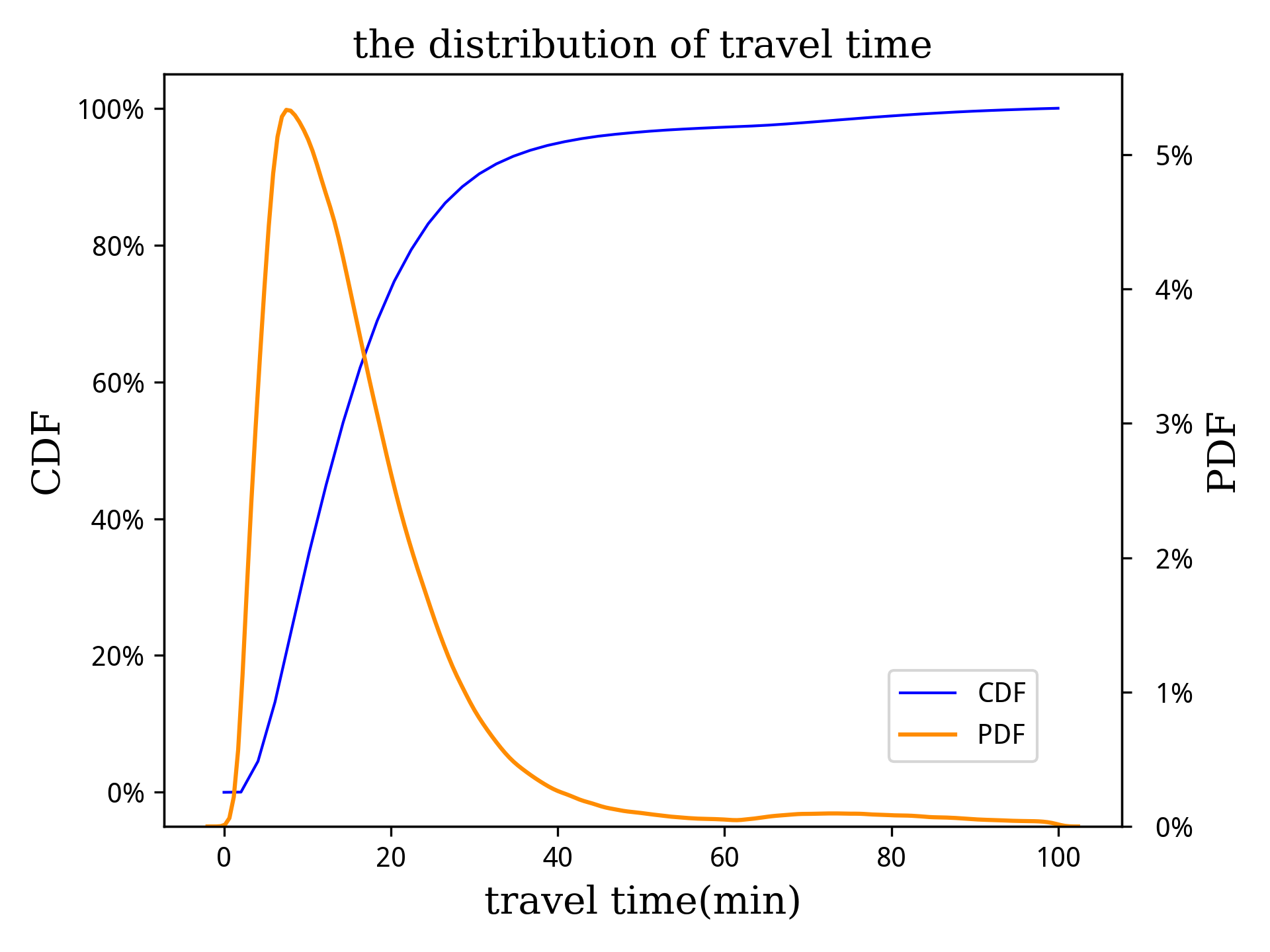
(a) Distribution of travel time of Chengdu dataset.

(b) Distribution of travel time of Porto dataset.

Figure 2: Distribution of travel time.

(a) Distribution of travel distance of Chengdu dataset.

(b) Distribution of travel distance of Porto dataset.

Figure 3: Distribution of travel distance.

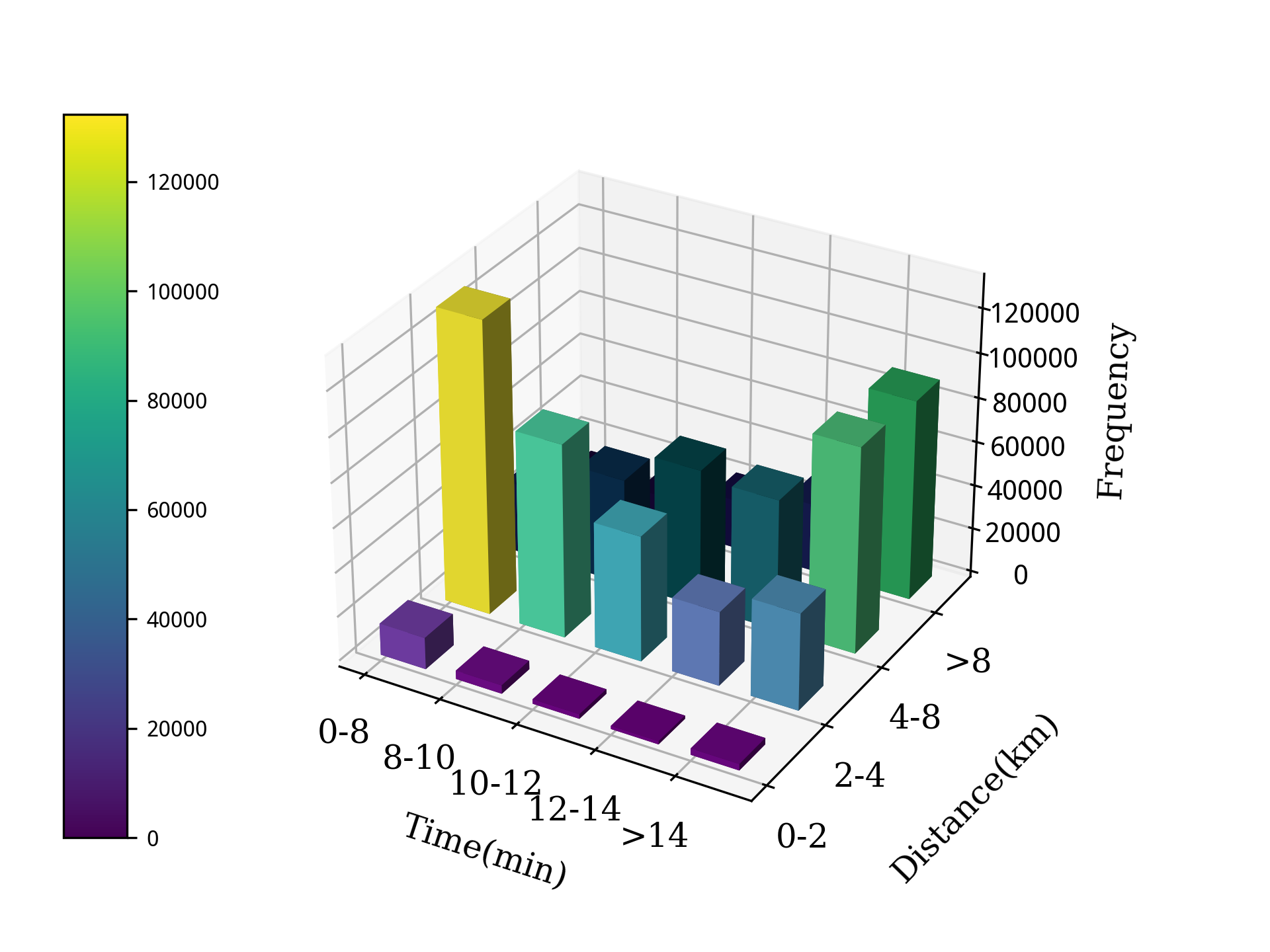
(a) Chengdu dataset.

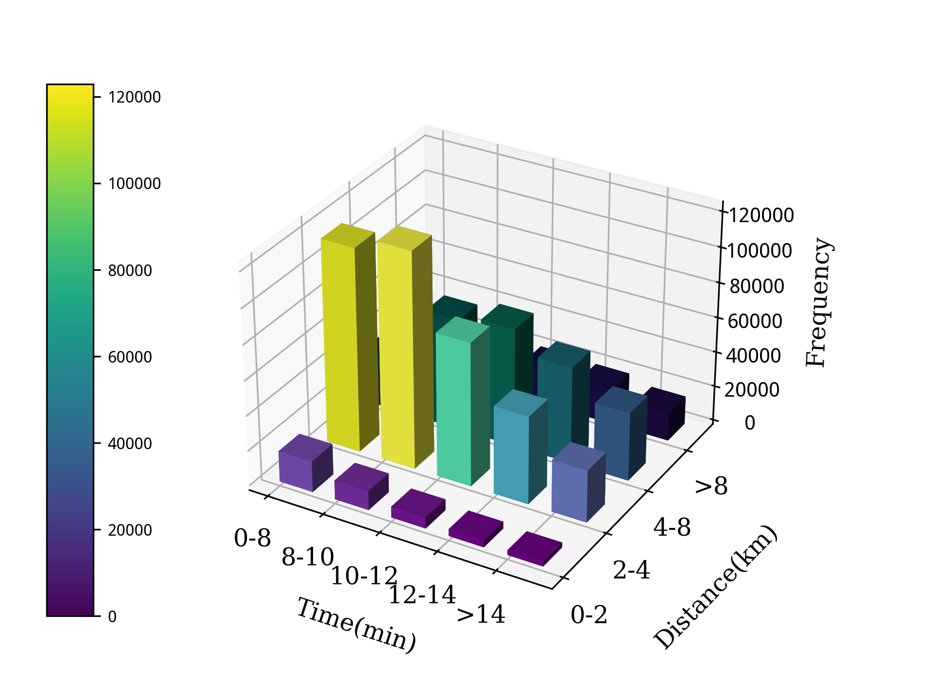
(b) Porto dataset.

Figure 4: Frequency of time and distance on Chengdu and Porto datasets (CDF from 10% to 80%).

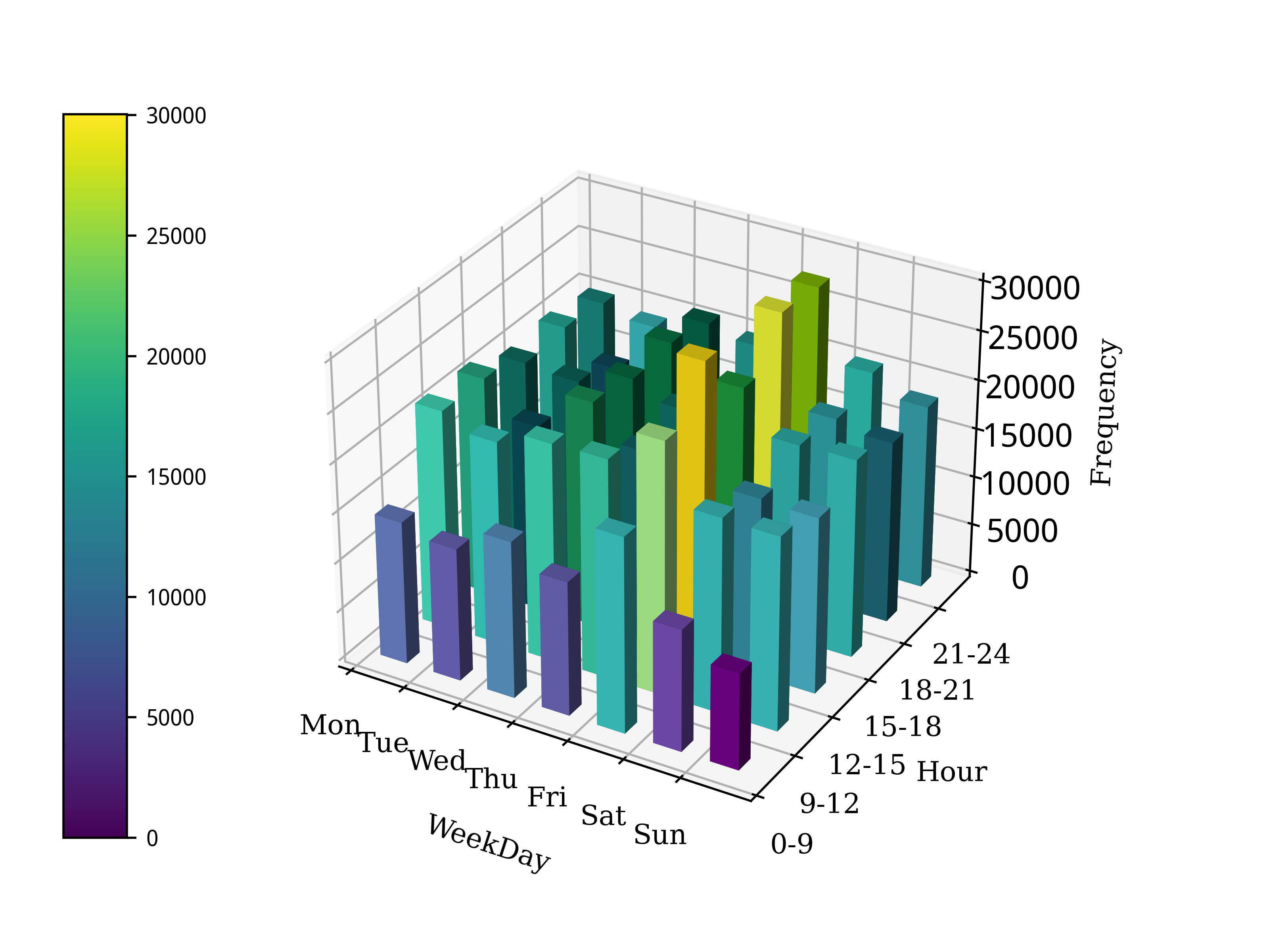
(a) Chengdu dataset.

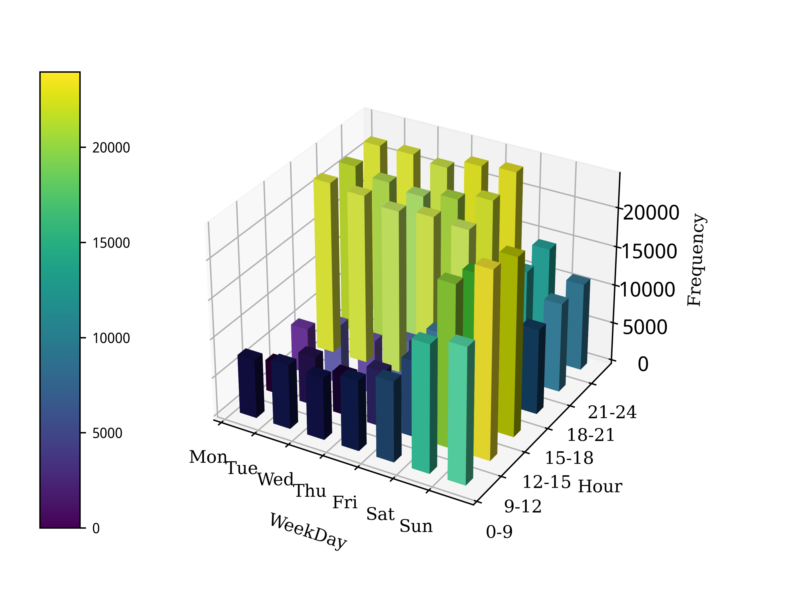
(b) Porto dataset.

Figure 5: Frequency of day of week and hour on Chengdu and Porto datasets (CDF from 10% to 80%).

We show the distribution of travel time of Chengdu and Porto datasets in Figure  2. Travel time on most trajectories (Cumulative Distribution Function (CDF) from 10% to 80%) in Chengdu dataset is between 315 seconds and 1174 seconds and that in Porto is between 315 seconds and 945 seconds. Meanwhile, as illustrated in Figure 3, travel distances on most trajectories (CDF from 10% to 80%) in Chengdu dataset are between 1.84 kilometers and 8.14 kilometers and that in Porto are between 1.76 kilometers and 7.32 kilometers. We thereby obtain available trajectories which fall into this range for our training phase and by this approach the dirty data or the abnormal data are removed. Furthermore, we also make more analysis on the Chengdu and Porto dataset to observe their data frequencies in different temporal and spatial domains. As illustrated in Figure 4, the distributions of data frequency of travel time and distance in Chengdu and Porto have some similarities which indicates that people are more likely to take taxi trips in the combination of travel time from 5 to 10 minutes and travel distance from 2 kilometers to 4 kilometers. However, Figure 5 shows that the distributions of data frequency of the combination of the day of week and hour in Chengdu and Porto are relatively different. People in Chengdu seems to take more taxi trips from the afternoon to evening on Friday, while people in Porto seems to take more taxi trips after 12:00 from Monday to Friday or from morning to nightfall on Sunday. These different patterns of taking taxi trips in multi-city scenarios may add difficulty to providing accurate travel time estimations.

IV Fine-grained Trajectory-based Travel Time Estimation Based on Deep Meta Learning

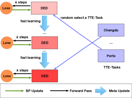
Figure 6: The framework of the proposed MetaTTE. The DED consists of data preprocessing module and encoder-decoder network module, which is marked with color pink, light red and dark red indicating the three continuous states of parameter initialization.

IV-A Overview

Figure 6 shows the framework of our proposed MetaTTE. For each iteration in the meta learning based training phase, a TTE-Task representing a unique region is randomly selected at first and then is fed into the DED for $k$ times steps of regular optimization. At the end of each iteration, an adaptive algorithm is adopted to change the initialization of parameters in DED in a fast learning manner.

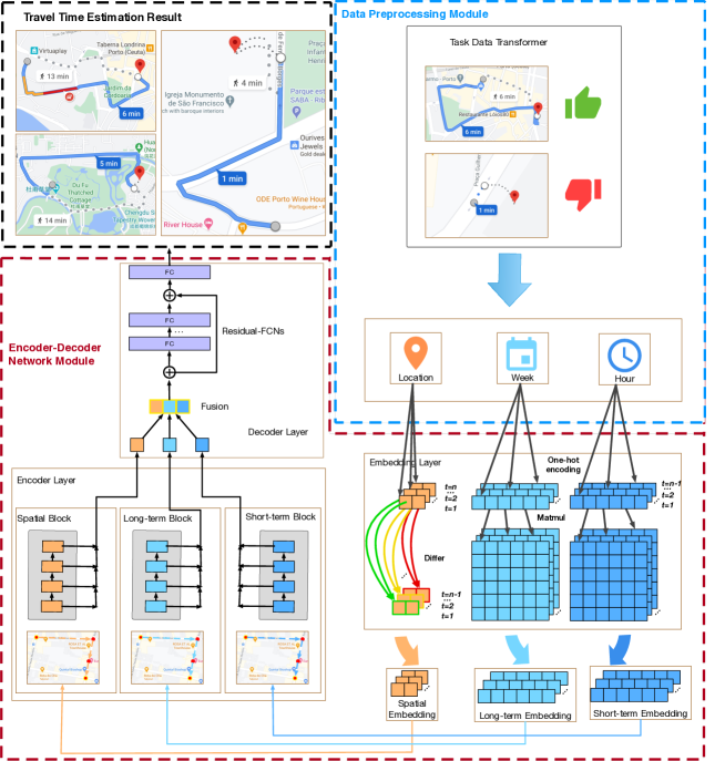
Figure 7: The architecture of DED.

IV-B DED

As illustrated in Figure 7, DED is composed of two components: the Data Preprocessing Module and the Encoder-Decoder Network Module. The Data Preprocessing Module is fed with the MetaTTE trajectory firstly, to remove the biases of outliers in real-world datasets and transform data into proper forms. Then the Encoder-Decoder Network Module is fed with the preprocessed DED trajectory data, to learn, encode the spatial-temporal representations and then decode the travel time estimations.

IV-B1 Data Preprocessing Module

The input pipelines are preprocessed in the Task Data Transformer and the preprocessed data are fed into the Encoder-Decoder Network Module.

Task Data Transformer. Meta learning only uses small amount of examples to train models for each iteration. To remove the biases of outliers in the real-world datasets and quickly adapt to new possible tasks, we set up several rules in the Data Preprocessing Module to dynamically control the input pipelines for DED.

• Rule 1: Keep the most frequent trajectory data only. After the deep insight into the analysis of our datasets, we decide only to keep trajectories which satisfied all the requirements listed in Table  III to ignore the rarely appeared samples to avoid possible biases when we train DED model using small amount of examples.

• Rule 2: Keep the trajectory if and only if it contains at least two different GPS points only. We regard that the isolated GPS point may be caused by occasional positioning errors and it is also nonsense to navigate users for the trajectory containing only one isolated GPS point.

• Rule 3: Keep the trajectory if and only if the total travel time is positive.

TABLE III: Satisfied requirements of Rule 1 for our datasets

Requirements	Chengdu	Porto
Travel Time No Less Than	315 seconds	315 seconds
Travel Time No More Than	1174 seconds	945 seconds
Travel Distance No Less Than	1.84 kilometers	1.74 kilometers
Travel Distance No More Than	8.14 kilometers	7.32 kilometers

IV-B2 Encoder-Decoder Network Module

The encoder-decoder network module mainly consists of three parts: the Embedding Layer, the Encoder Layer and the Decoder Layer. The preprocessed input data are firstly embedded into low dimensional feature vectors in the Embedding layer and then different embeddings are encoded separately in the Encoder layer through RNN. After that, the separate spatial and temporal encoded feature representations are fused using Attention Mechanism and then decoded using residual fully connected layers (Residual FCs) in the Decoder Layer. And finally travel time estimations are made based on the decoded feature representations.

Embedding Layer. In the embedding layer, we embed the the day of week and hour which are represented with categorical values into low dimensional real vectors, which allows neural network to conduct feature learning on our real-world datasets. To better represent the temporal patterns for travel time estimation, we choose a word embedding method mentioned in  [21] which maps each categorical value $c\in[C]$ in one-hot encoding to the embedding space (i.e. a real space) $\mathbb{R}^{E\times 1}$ by multiplying a trainable parameter matrix $W\in\mathbb{R}^{C\times E}$ with the initial values of all zeroes and then the parameter matrix is optimized using the meta-learning based gradient descent algorithm  [22].

In order to enhance the scalability of our model, all factors including the day of week, hour are separately embedded to different channels, and the output for each factor is formulated as:

$$e=\phi(x)\mathcal{W}^{T}$$ (2)

where $\phi(\cdot)$ represents the mapping function for one-hot encoding, $x$ is the factor vector (i.e. the day of week and hour) and $\mathcal{W}$ is the parameter matrix for feature learning. In this paper, the differences of the GPS coordinates (i.e. $(\Delta p_{1},\Delta p_{2})$), the embedding of the the day of week and the embedding of the hour are adopted to represent the spatial embedding ($e_{p}$), the long-term embedding ($e_{w}$) and the short-term embedding ($e_{h}$) respectively and are fed into the encoder layer for fine-grained feature learning.

Encoder Layer. As mentioned in Section I, it is significant to capture fine-grained spatial dependencies in daily scenarios for achieving satisfied travel time estimation. Some studies [10] firstly apply convolutional layers to learn local-path features and then feeds local-path features into recurrent layer to further learn the entire-path features. However, since the size of kernels in the convolutional layer are fixed, the receptive field of local-path features learnt in this layer are also limited to fixed range. This prevents the model to learn fine-grained spatial features smaller than the size of kernels or larger than the size of kernels. To address this issue, we design fully RNN based blocks to encode the spatial embeddings, long-term embeddings, and short-term embeddings. Notice that DED supports user-specific blocks for better scalability. It’s simple to add or remove several blocks when needed since we employ feature learning in separate channels and this will not influence the other parts of DED. Since state-of-the-art RNNs have been widely investigated, we conduct extensive experiments on several common RNNs, including LSTM  [23], GRU [24] and BiLSTM  [25]. The update rule of each RNN is formulated as:

$$(\mathcal{C}^{t},\mathcal{Y}^{t})=RNN(e^{t},\mathcal{C}^{t-1},\mathcal{Y}^{t-1})$$ (3)

where $\mathcal{C}^{t}$ is the updated hidden state and $\mathcal{Y}^{t}$ is the updated output. Notice that there is no memory cell $\mathcal{C}$ in GRU and we regard the $\mathcal{Y}$ as the hidden state instead.

In this paper, we utilize the hidden states $C^{t}_{p},C^{t}_{w},C^{t}_{h}$ when $t=l$ as the learnt spatial-temporal features of spatial embedding, long-term embedding and short-term embedding to transform variable length embeddings into encoded fixed-length representations.

Decoder Layer. In the Decoder Layer, we first fuse the encoded spatial-temporal features using Attention Mechanism and then decode the fused spatial-temporal representations in Residual FCs.

• Attention mechanism. To aggregate the encoded spatial-temporal features containing fine-grained spatial dependencies, a self-attention mechanism [26] is adopted to learn the importance of different dimensions in each type of feature and aggregate them to obtain fused spatial and temporal representations. We first concatenate all the spatial-temporal features (i.e. $\mathcal{C}_{p},\mathcal{C}_{w},\mathcal{C}_{h}$) and then design a score function to automatically assign importance to different dimensions which is formulated as:

  $$\mathcal{S}=\max(0,((\mathcal{C}_{p}||\mathcal{C}_{w}||\mathcal{C}_{h})\mathcal{W}+b))$$ (4)

  where $\mathcal{C}_{p},\mathcal{C}_{w},\mathcal{C}_{h}\in\mathbb{R}^{N\times D}$ ($D$ is a hyper-parameter which indicates the output dimension of the embedding layer), $||$ represents the concatenation operation, $\mathcal{S}$ represents the contribution score for different dimensions in each feature, $\mathcal{W}\in\mathbb{R}^{N\times F\times F}$ ($F=3$) and $b$ are trainable parameters. Once obtaining the scores for different dimensions, we normalize the score $\mathcal{S}^{i}$ for $i^{th}$ feature using the softmax function to obtain the attention values which can be formulated as:

  $$a_{i}=Softmax(\mathcal{S}_{i})=\frac{\exp(\mathcal{S}_{i})}{\Sigma_{i}\exp(\mathcal{S}_{i})}$$ (5)

  where $a_{i}$ is the attention value for the $i^{th}$ feature of each dimension. We calculate the fused spatial and temporal features for travel time estimation formulated as:

  $$\mathcal{C}_{f}=\Sigma_{i=1}^{F}a_{i}\odot{(\mathcal{C}_{p}||\mathcal{C}_{w}||\mathcal{C}_{h})}_{i}$$ (6)

  to obtain the fused spatial-temporal representation $\mathcal{C}_{f}\in\mathbb{R}^{N\times D}$.

• Residual FCs. In practice, FCs are commonly used to decode the spatial-temporal representations in higher level. Since the residual technique can accelerate the training process [27], we build residual blocks with four FCs to decode the spatial-temporal representations and enhance the performance without consuming much time. We formulate this process as:

  $$\mathcal{Y}_{estimation}=FC_{estimation}(FCs(\mathcal{C}_{f})+\mathcal{C}_{f})$$ (7)

  where $FC_{i}(\mathcal{Y})=\mathcal{Y}\mathcal{W}_{i}^{T}+b$, $\mathcal{W}_{i}$ is the trainable parameter matrix for the $i^{th}$ fully connected layer and

  $$FCs(\mathcal{C}_{f})=FC_{1}(FC_{2}(FC_{3}(FC_{4}(\mathcal{C}_{f})))).$$ (8)

IV-C Meta Learning based Optimization Algorithm

Inspired by Reptile [18], which works by repeatedly sampling a task, training on it and moving the initialization towards the trained parameters on that task and has achieved good results on some well-established benchmarks, we introduce the Reptile algorithm to optimize MetaTTE, which is shown schematically in Figure 8 and the pseudocode of the detailed algorithm is shown in Algorithm 2.

The inputs of Algorithm 2 are TTE-tasks $p_{\mathcal{T}}$, model $\mathcal{M}$ which contain the hyperparameters $\lambda$ and the trainable parameters $\theta$ and the loss function for task $\mathcal{T}_{i}$: $\mathcal{L}_{\mathcal{T}_{i}}$. We first set a proper value for the maximum iteration $\eta$ to declare the stopping criteria of the training phase. From experiments, our MetaTTE can converge to the satisfied MAE (Mean Absolute Error) metrics within 7000 iterations (i.e. $\eta=7000$). For each iteration in the training phase, we firstly prepare datasets for training (Line 3). In the training phase, we first save the current model parameters to $\theta_{1}$ (Line 4) and then sample $k$ batches of training data and conduct forward-backward propagation using gradient descent based algorithm, Adam [28], to minimize the loss $\mathcal{L}_{\mathcal{T}_{i}}$ for optimization (Line 5$\sim$9). The model parameters after $k$ times of optimizations are saved in $\theta_{2}$ (Line 10). Then we conduct the meta update on MetaTTE and calculate $\theta_{f}$ (Line 11). Similar to Reptile, we develop the adaptive algorithm as a linear learning rate scheduler [29] formulated as:

$$\theta_{f}=\beta(1-\frac{r}{\eta})(\theta_{2}-\theta_{1})$$ (9)

where $\beta$ is the step size for learning rate scheduling, $\eta$ is the maximum iteration times, $r$ is the current training iteration, $\theta_{1}$ and $\theta_{2}$ are the parameters before and after $k$ times of training steps, respectively. At last, the model parameters are reset to $\theta_{f}$ (Line 12) to accomplish optimization in this iteration.

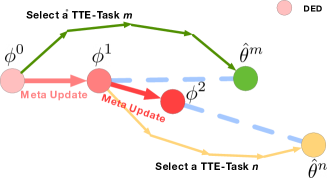
Figure 8: The schematic of the optimization algorithm for MetaTTE. Three circles marked with pink, red and dark red represent the continuous states of the initializations for trainable parameters in DED. Assume we firstly select TTE-Task $m$ and conduct 10 times gradient calculations to derive the parameters $\hat{\theta}^{m}$ (marked with green). Instead of arbitrarily updating the model using $\hat{\theta}^{m}$ at once, we conduct once meta-update which utilizes an adaptive algorithm to update the model parameters $\phi^{0}$ to $\phi^{1}$ based on $\hat{\theta}^{m}$. Then we select TTE-Task $n$ and conduct the same operations (marked with yellow) to update model parameters to $\phi^{2}$. This deferred update pattern helps MetaTTE pay more attention to the potential of providing accurate estimation further in the future.

Input : TTE-Tasks $p_{\mathcal{T}}=\{\mathcal{T}_{1},\mathcal{T}_{2}\}$, model $\mathcal{M}$, loss function for task $\mathcal{T}_{i}$: $\mathcal{L}_{\mathcal{T}_{i}}$.

Output : A partition of the bitmap

1 randomly initialize $\theta$;

2 for $r$ in $[1,\eta)$ do

3       // multi-city task selection ;

4       Randomly select a TTE-Task $\mathcal{T}_{i}$ from $p_{\mathcal{T}}$;

5       Save current model parameters to $\theta_{1}$ ;

6       for j in $[1,k]$ do

7             $\mathcal{X}_{train},\mathcal{Y}_{train}$ $\leftarrow$ Sample data from $\mathcal{D}_{\mathcal{T}_{i}}^{train}$ ;

8             $\hat{\mathcal{Y}}$ $\leftarrow$ $\mathcal{M}(\mathcal{X}_{train})$ ;

9             Update model parameters using Adam on $\mathcal{L}_{\mathcal{T}_{i}}$;

10            

11       end for

12      Save current model parameters to $\theta_{2}$ ;

13       Calculate model final parameters $\theta_{f}$ using $\theta_{1},\theta_{2}$;

14       Reset model parameters to $\theta_{f}$ ;

15      

16 end for

Algorithm 2 Optimization algorithm for MetaTTE.

V Experiments

In this section, we evaluate our proposed MetaTTE and compare it with six baseline approaches based on Chengdu and Porto datasets.

V-A Baselines

AVG. [12] This method calculates the average speed with the travel time and the taxicab geometry in the training phase. During the test phase, the estimation is calculated by averaging the historical speeds of those with the same origin and destination.

LR [12]. This method trains the relation between the taxicab geometry and travel time based on the locations of origin and destination.

GBM [12]. This method utilizes the departure time, the day of week, GPS coordinates and taxicab geometry to provide travel time estimation using gradient boosting decision tree models.

TEMP [30]. This method estimates the travel time based on the average travel time using neighboring trips from large-scale historical data.

WDR [3]. This deep learning based method extracts handcrafted features from raw trajectory data and utilizes information extracted from road segments to provide travel time estimations.

DeepTTE [10]. This method learns spatial and temporal feature representations from raw GPS trajectories and several external factors using 1-D convolutional and LSTM networks.

STNN [31]. This method firstly predicts the travel distance between an origin and a destination GPS coordinate, and then combines this prediction with the time of the day to predict travel time using fully connected neural networks.

MURAT [32]. This method utilizes multi-task representation learning to jointly learn the main task (i.e. travel time estimation) and other auxiliary tasks (i.e. travel distance etc.) and enhances the performance for travel time estimation.

Nei-TTE [11]. This method divides the entire trajectory into multiple segments and captures features from road network topology and speed interact using GRU for travel time estimation.

MetaTTE-WA. The variant of MetaTTE, which utilizes LSTM as the RNN layer without attention based fusion.

MetaTTE-WT. The variant of MetaTTE, which utilizes LSTM as the RNN layer without short-term and long-term embeddings.

MetaTTE-LSTM. The variant of MetaTTE, which utilizes LSTM as the RNN layer.

MetaTTE-BiLSTM. The variant of MetaTTE, which utilizes BiLSTM as the RNN layer.

MetaTTE-GRU. The variant of MetaTTE, which utilizes GRU as the RNN layer.

V-B Experimental Settings

In this part, we first introduce the configurations of our evaluation environment briefly and then describe the hyperparameters in our MetaTTE.

V-B1 Configurations

We utilize the TensorFlow framework to implement, train, validate and test our proposed MetaTTE. We conduct our evaluations on a node of the Dawn supercomputer with the CPU (Intel E5-2680 2.4GHz x 28), RAM (64GB), GPU (Tesla V100S 32GB), Operating System (Centos 7.4) and deep learning framework (TensorFlow 2.3). During the test phase, we train 100 epochs for each baseline using fine-tuned hyperparameters on Chengdu and Porto datasets respectively and compare the results with our MetaTTE. Notice that conventional deep learning methods optimize parameters on all batches of data for each epoch, while our MetaTTE optimize parameters on small amount of data for each iteration, which is much faster than the former.

V-B2 Hyperparameters

The hyperparameters for MetaTTE can be categorized into two parts: (i) training hyperparameters which includes batch size (32), step size $\beta(0.1)$, $k$ (10) batches of training data, maximum iteration $\eta$ (7000); (ii) model hyperparameters which include the dimension of embedding $D$ (64), the number of units in RNN $n_{r}$ (64), and the number of units in residual FCs (1024, 512, 256, 64 respectively). Additionally, all the trainable parameters in the model are initialized using Xavier initialization method.

TABLE IV: Performance comparison of different baselines for travel time estimation on Chengdu and Porto datasets. Notice that all metrics are calculated based on travel time in seconds.

Baselines	Chengdu			Porto
	MAE	MAPE (%)	RMSE	MAE	MAPE (%)	RMSE
AVG	442.20	39.71	8443.60	182.64	26.66	1128.21
LR	516.23	49.09	1204.99	194.40	33.90	279.20
GBM	454.50	41.67	1121.32	148.53	24.59	209.07
TEMP	334.60	39.70	761.05	174.44	28.73	260.81
WDR	433.99	29.74	1024.92	164.04	22.84	244.41
DeepTTE	413.09	24.22	926.04	84.29	14.79	90.29
STNN	427.33	30.08	1011.88	226.30	35.44	331.75
MURAT	396.01	29.29	994.95	165.91	27.10	177.83
Nei-TTE	414.16	30.04	1038.71	106.30	15.23	183.03
MetaTTE-WT	264.55	33.12	792.39	69.87	9.98	203.29
MetaTTE-WA	258.10	27.16	774.87	68.16	9.84	204.64
MetaTTE-LSTM	249.47	24.97	757.87	65.88	9.35	200.15
MetaTTE-BiLSTM	254.47	25.55	766.45	67.20	9.59	202.42
MetaTTE-GRU	236.38	23.69	745.11	62.43	8.83	196.78

V-B3 Experimental Results

In this part, we first compare the results among variants of MetaTTE and all of six baselines. We firstly introduce the evaluation results using all the baselines on overall datasets. Then in order to investigate the impacts of different travel time and travel distances to estimation performance, we conduct extensive experiments of baselines on two datasets. We then show our fine-tuning results when investigating the impact of the hyperparameters. Lastly, we conduct ablation studies on our MetaTTE.

Comparing to all the baselines on Chengdu and Porto dataset. Table IV compares the performance of different baselines on two datasets. We can observe that: (1) deep learning based methods outperform other traditional time series methods in MAPE metric, which indicates the superior of its ability to learn dynamic temporal features and fine-grained spatial features for travel time estimation; (2) MetaTTE-GRU outperforms other baselines in MAE and MAPE metrics on two datasets. The reason for the increase in RMSE metric on Porto dataset compared with DeepTTE may lie in: (i) instead of training two separate models for Chengdu and Porto like DeepTTE does, MetaTTE-GRU trains only single model for both datasets of Chengdu and Porto which may be slightly influenced by the volatile datasets; (ii) some outliers in datasets (rarely appeared samples with CDF below 10% or above 80%) influence the RMSE metric since MetaTTE-GRU is fed with the raw trajectory data, while DeepTTE is fed with the resampled trajectory data which reduces the influence of outliers. Since the MAPE metric is more important in real-applications for the fact that the user tolerance of the estimation gap varies according to total travel time [3] and the objective of the applications is to satisfy users in majority, MetaTTE-GRU still outperforms other baselines; (3) The variants of MetaTTE significantly outperforms other baselines on Porto dataset, which indicates the strong generalization ability of MetaTTE to continuously provide accurate travel time estimation further in the future.

Impact of different travel time. In order to investigate the impact of different travel time on MetaTTE comparing to selected baselines, we conduct extensive experiments on different parts of the test datasets of both Chengdu and Porto. Specially, we utilize MetaTTE-GRU which can outperform other baselines using overall datasets in this study. As illustrated in Figure 9, MetaTTE-GRU achieves the best performance in MAE and RMSE metrics in different travel time except for the MAPE metric of the travel time which is more than 14 minutes. According to the analysis of the data in Section III, it is reasonable to regard these trajectory data as the occasional events or the dirty data having be removed with the constraints of Rule 1 in the data preprocessing module when training our model and this has made this part of trajectory data the unseen dataset to our MetaTTE-GRU model. Therefore, under such circumstances, MetaTTE-GRU can provide relatively better estimation results in MAE and RMSE metrics which demonstrates the good generalization ability for fault tolerance of MetaTTE-GRU to some extent. In a similar way, as shown in Figure 10, the performance of MetaTTE-GRU on Porto dataset is better than other baselines in MAE and MAPE metrics.

Impact of different travel distances. We further investigate the impact of different travel distances on MetaTTE-GRU and selected baselines. Similar with the discussions made when investigating the impact of different travel distances, Figure 11 and Figure 12 show that MetaTTE-GRU achieves best performance in most of the metrics (i.e. MAE and RMSE metrics) except for the MAPE metric on occasional events which is higher than other baselines. Moreover, if we look into the estimation results of TEMP, which is path-based methods, the MAPE metric varies a lot when being tested on the most frequent travel distance data and the rarest travel distance data which may indicate the poor fault tolerance ability TEMP has. In a similar way, MURAT and DeepTTE may face the same pitfalls while MetaTTE-GRU may not vary a lot in MAPE and RMSE metric when being tested on those types of data and, especially, MetaTTE-GRU is trained on two datasets with only single model which may be more likely biased than other baselines which are trained as two individual models for two datasets.

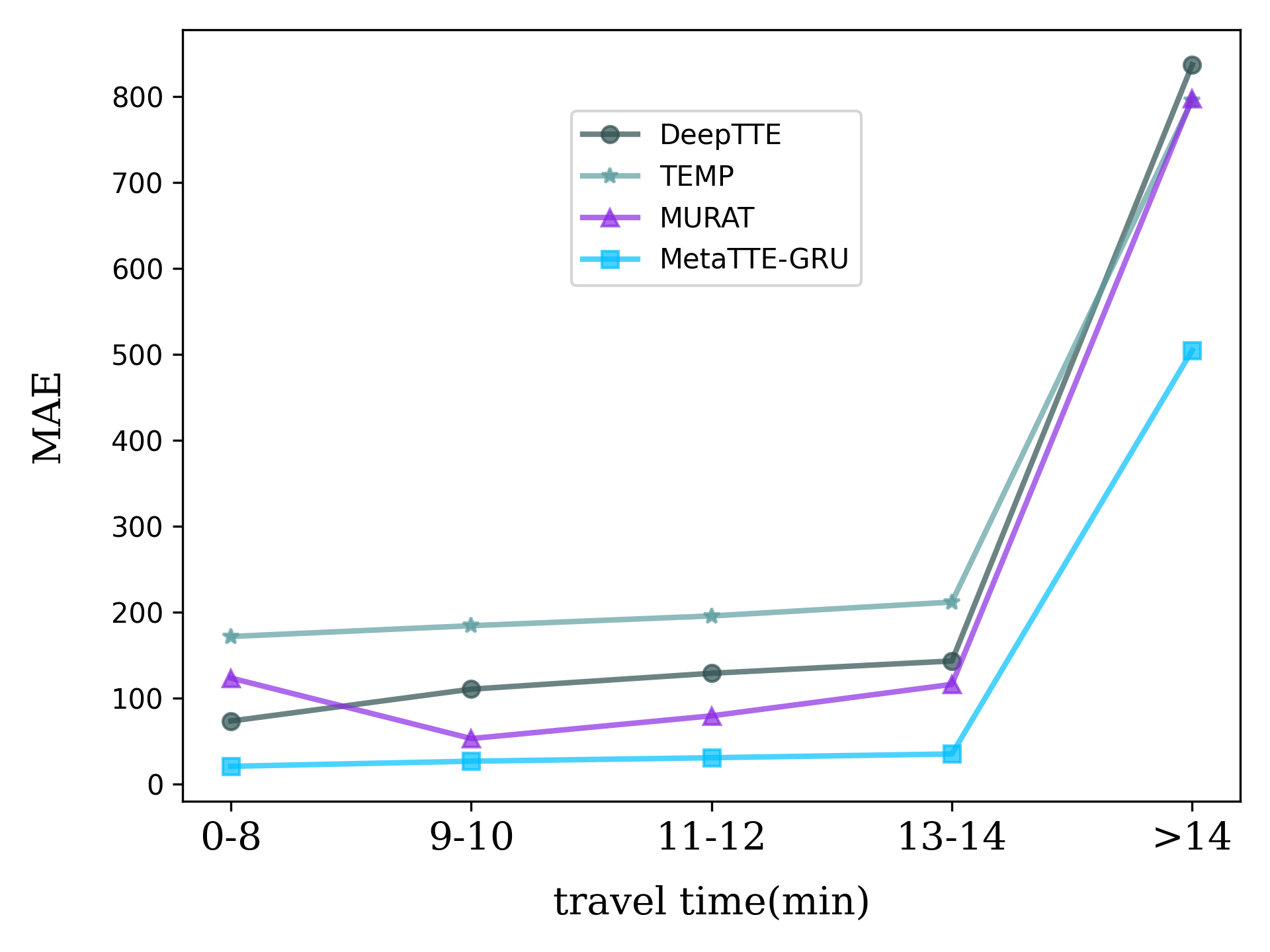
(a) MAE metric.

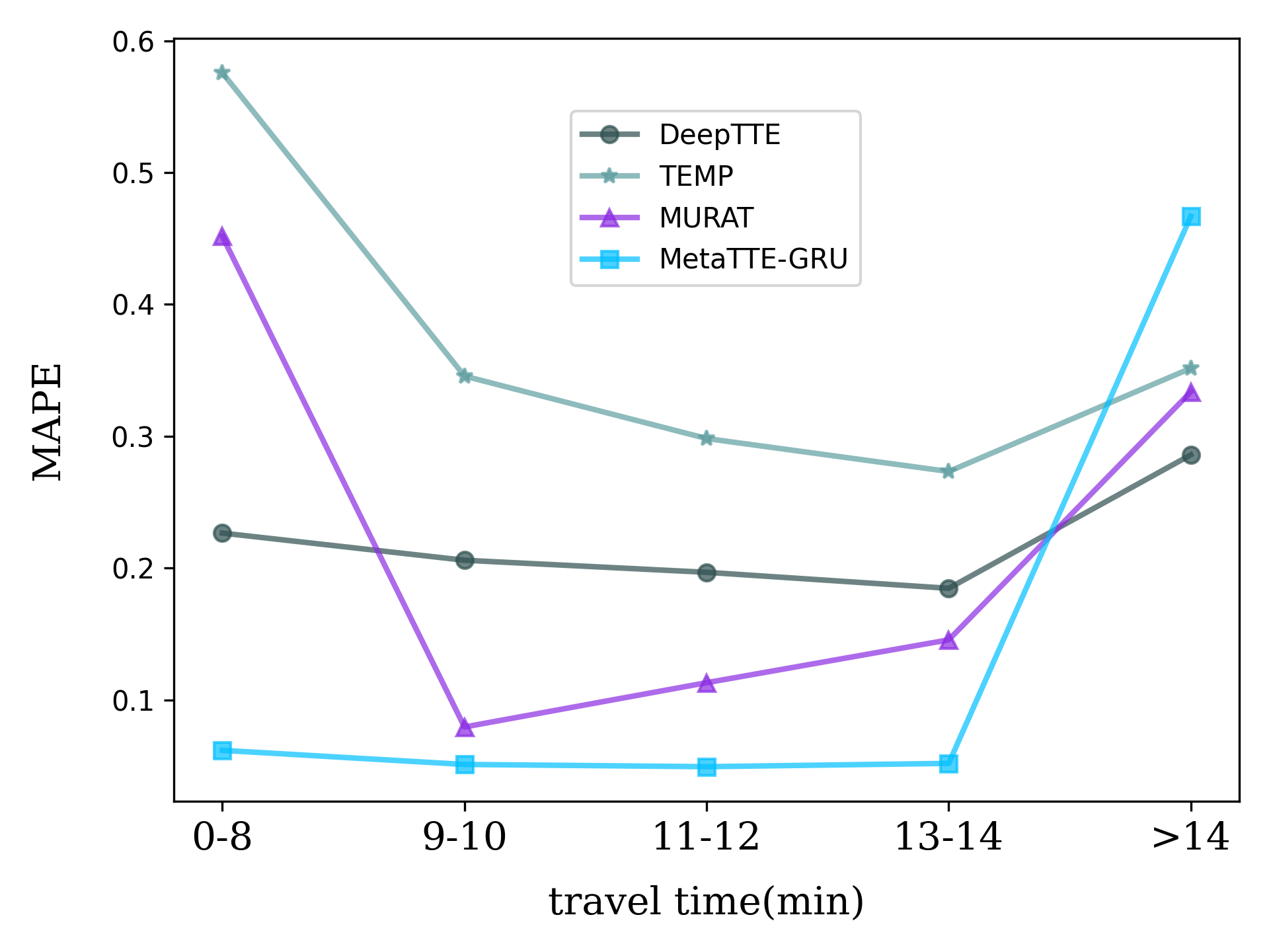
(b) MAPE metric.

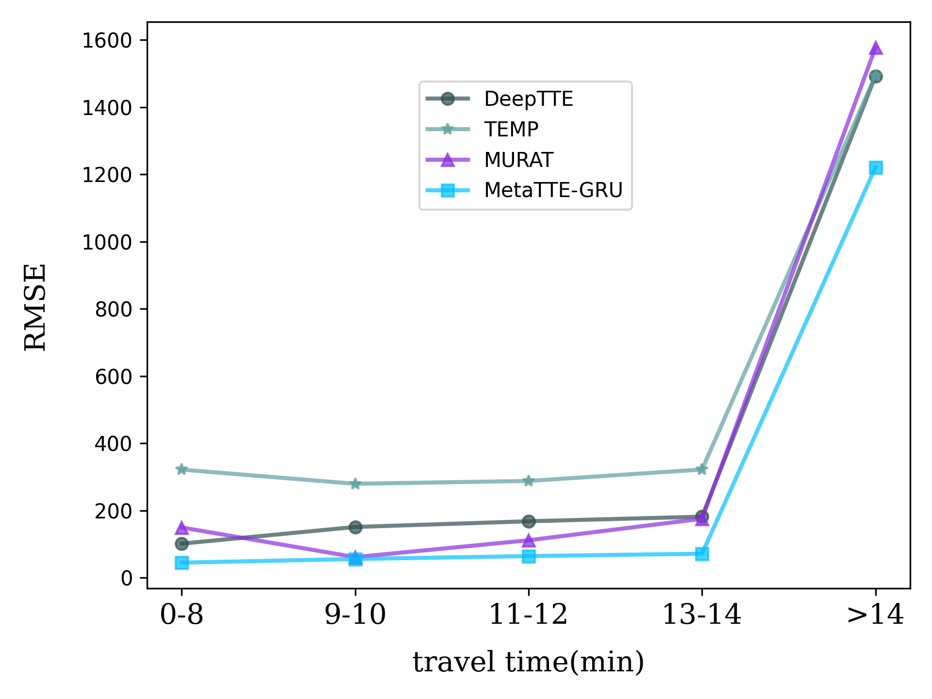
(c) RMSE metric.

Figure 9: MAE, MAPE and RMSE metric results on Chengdu datasets of different travel time.

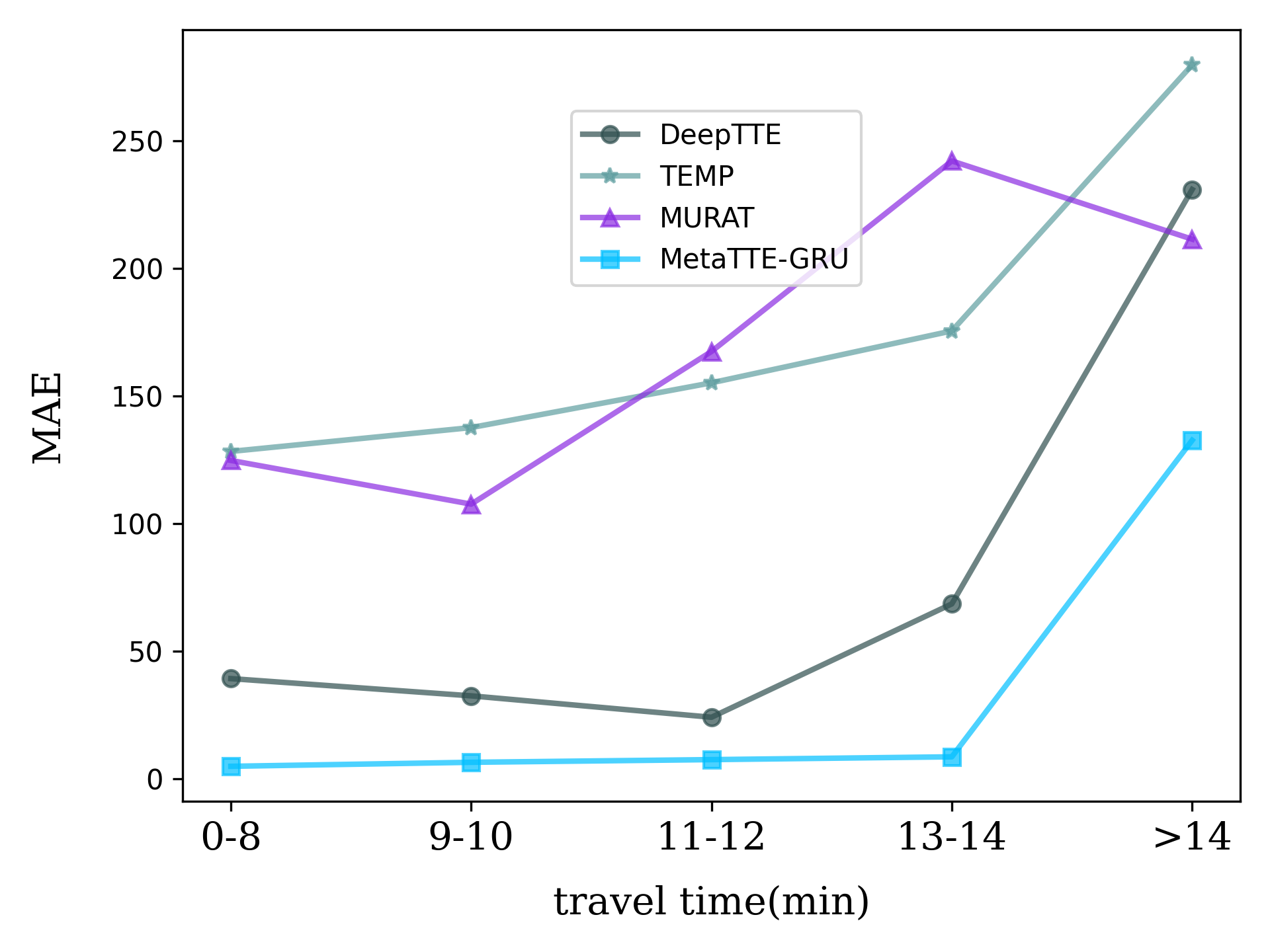
(a) MAE metric.

(b) MAPE metric.

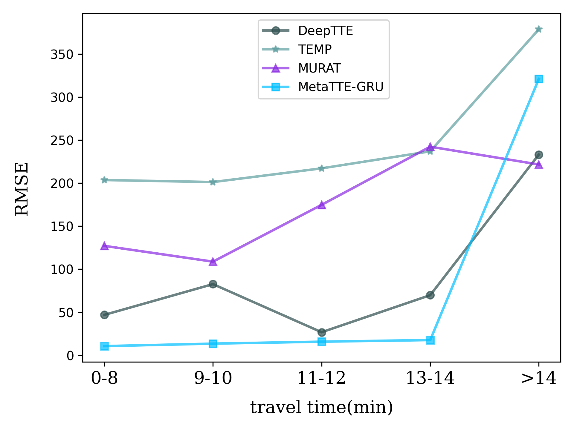
(c) RMSE metric.

Figure 10: MAE, MAPE and RMSE metric results on Porto datasets of different travel time.

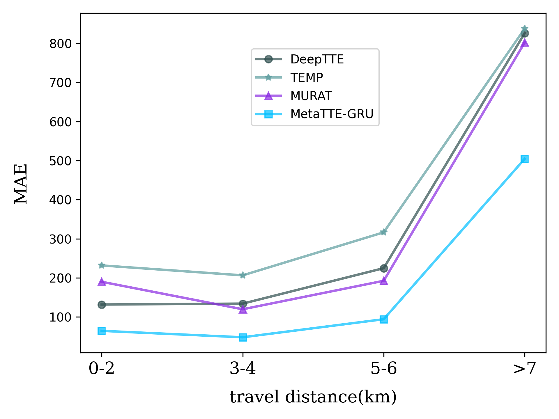
(a) MAE metric.

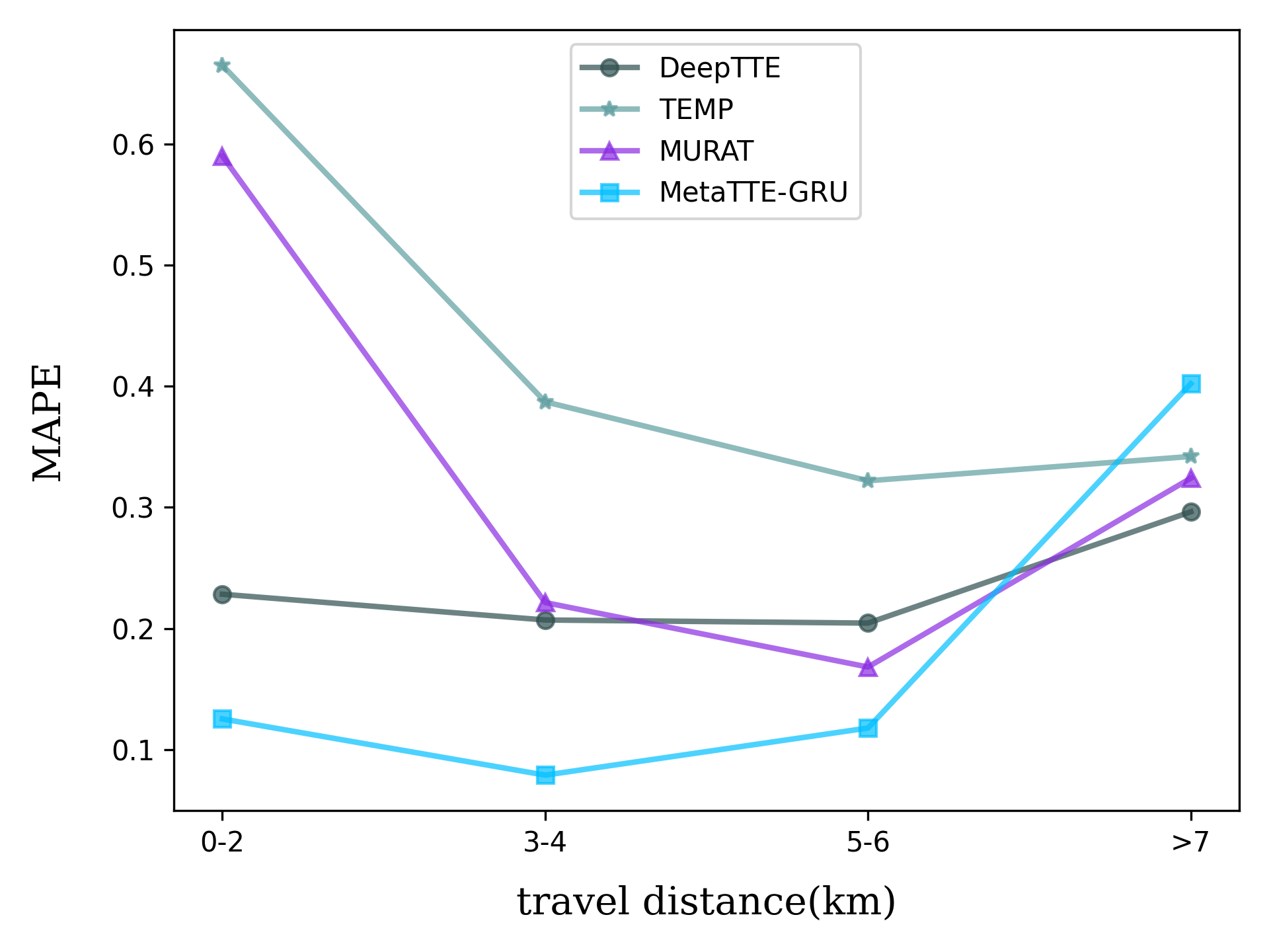
(b) MAPE metric.

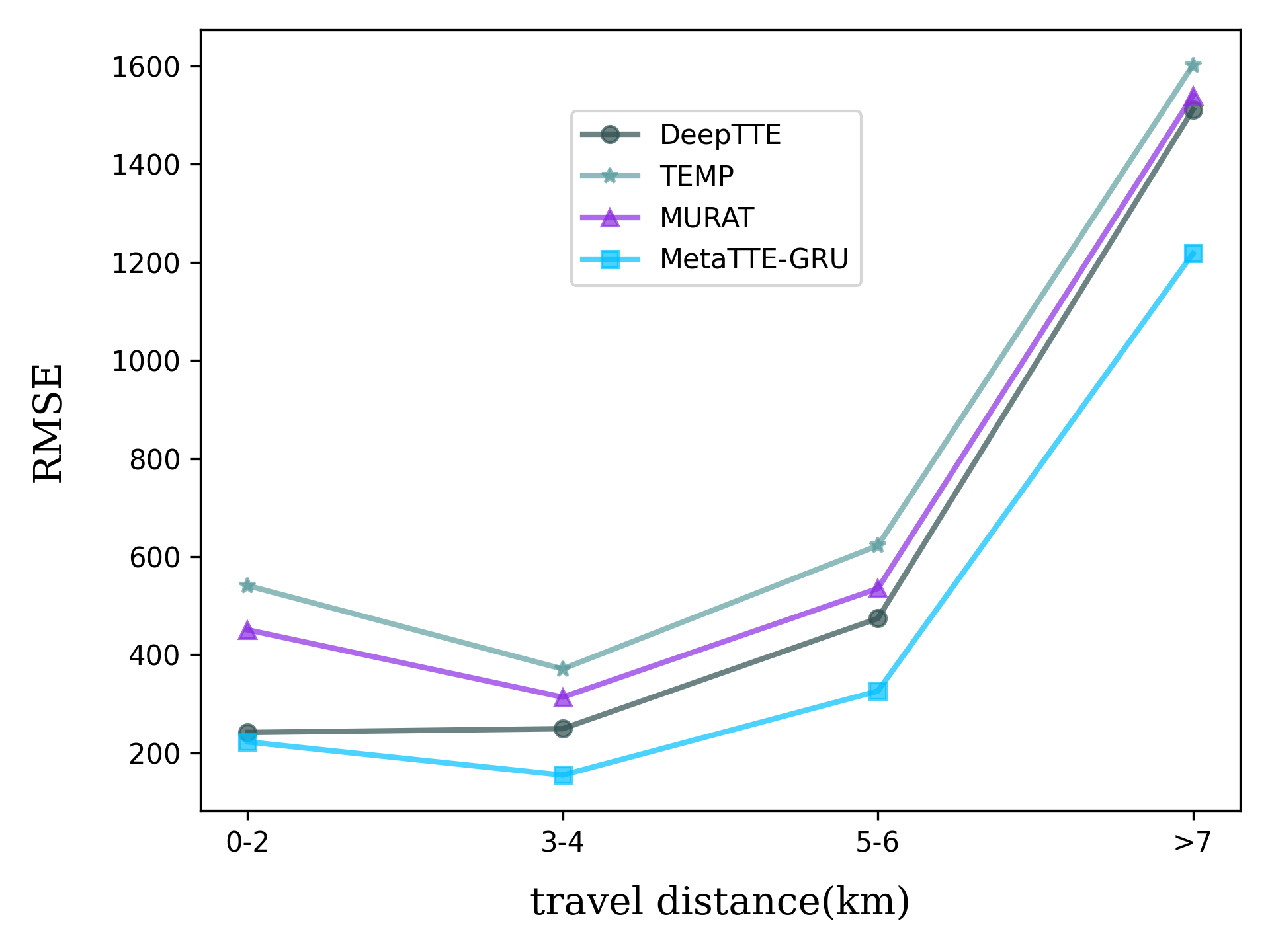
(c) RMSE metric.

Figure 11: MAE, MAPE and RMSE metric results on Chengdu datasets of different travel distances.

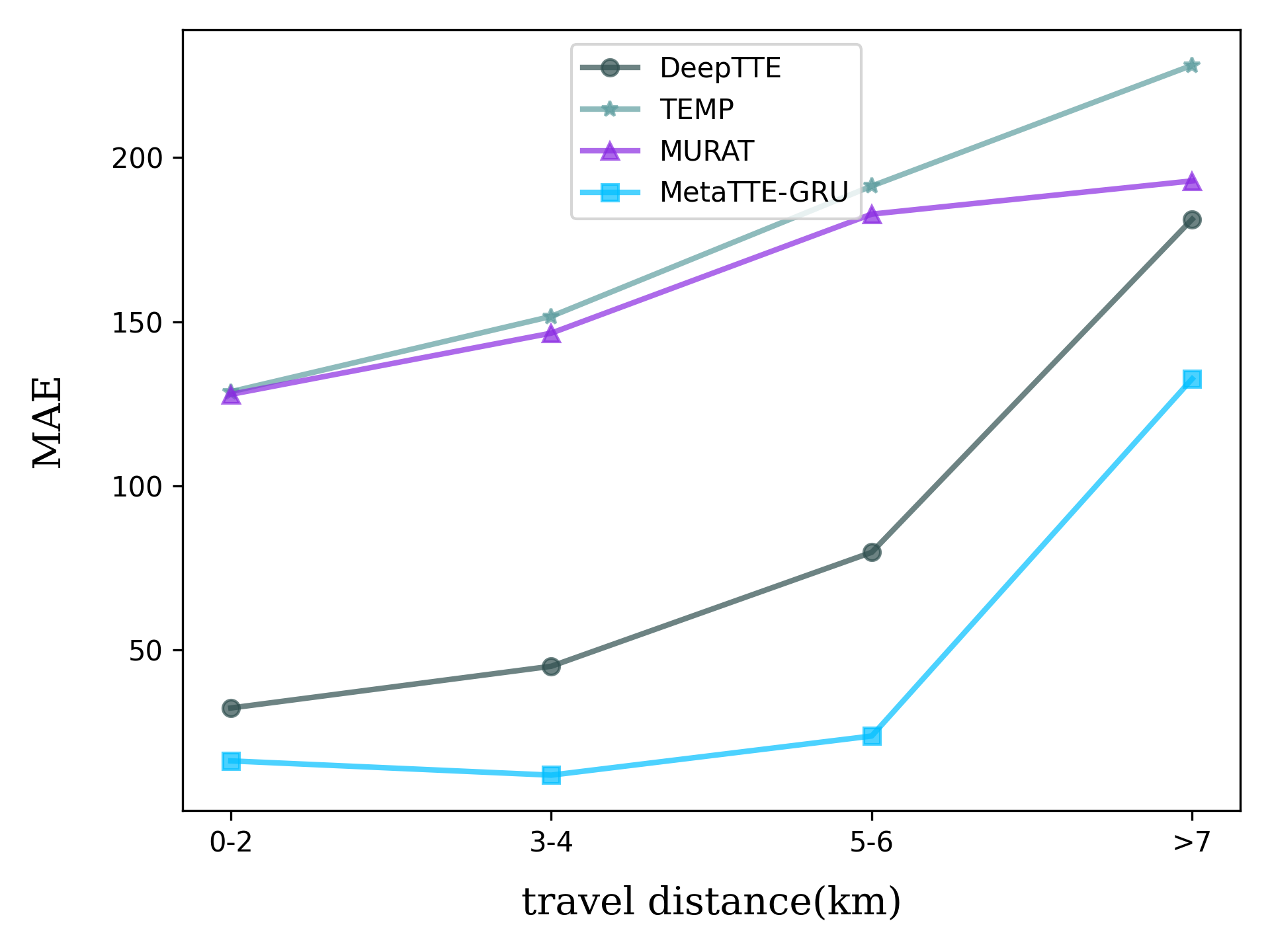
(a) MAE metric.

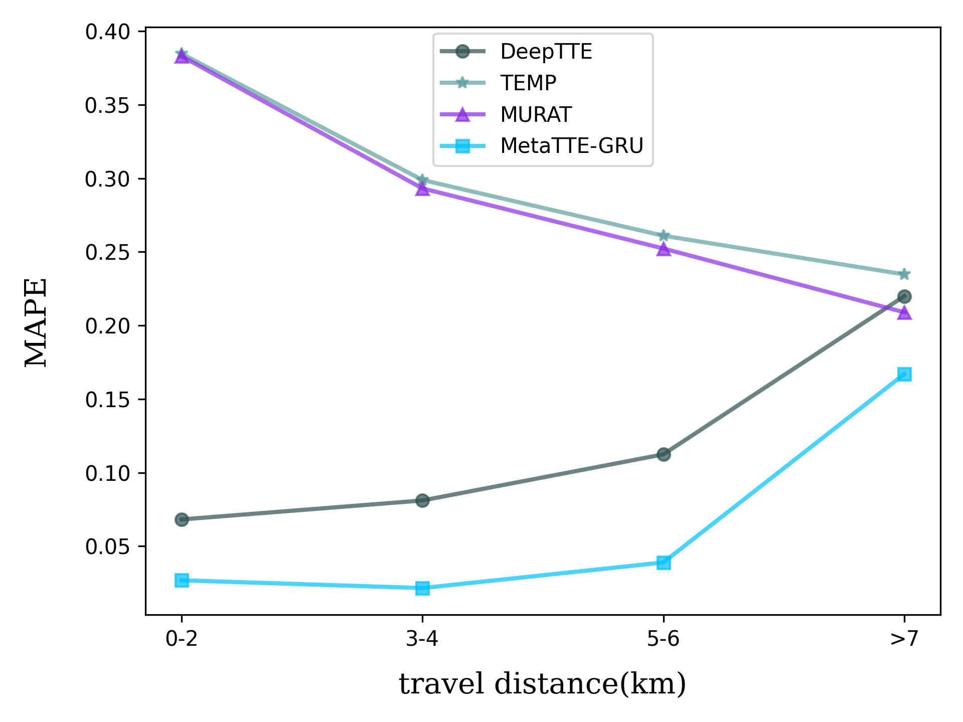
(b) MAPE metric.

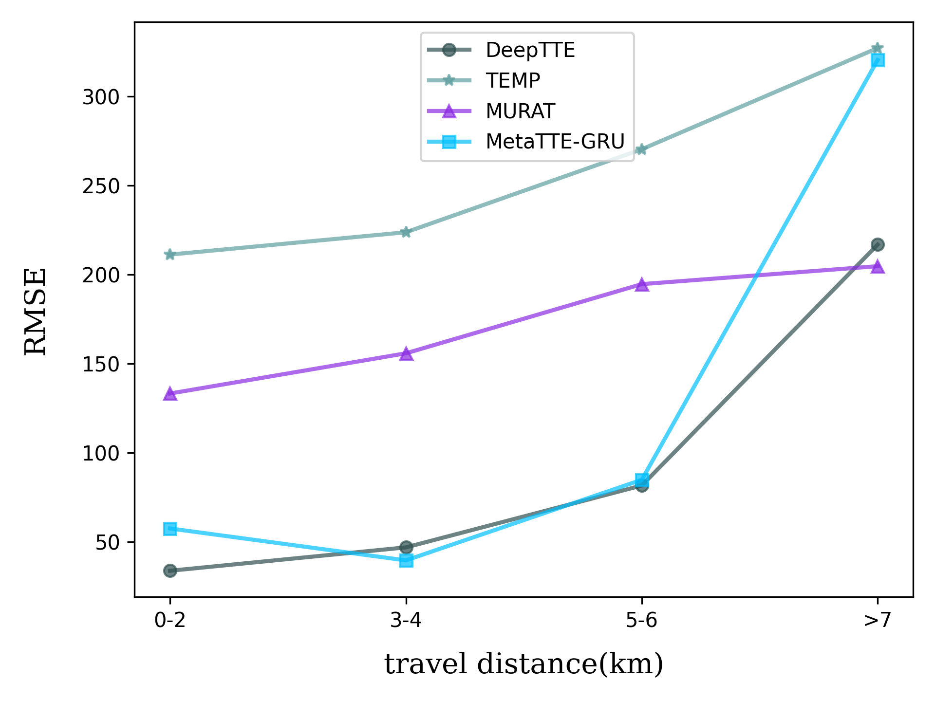
(c) RMSE metric.

Figure 12: MAE, MAPE and RMSE metric results on Porto datasets of different travel distances.

V-B4 Impact of different hyperparameters.

In order to investigate the impact of different hyperparameters and finetune our proposed MetaTTE, we conduct experiments using different training and model hyperparameters. Specially, we conduct experiments based on MetaTTE-LSTM which is also the baseline we adopted in ablation studies. We then describe the results.

• Training hyperparameters. The most important hyperparameter in our settings is the step size $\beta$ which schedules the learning rate for our meta-learning based optimization algorithm and thus we further investigate training hyperparameter and show the results in Table V. We can observe that the MAE, MAPE and RMSE metrics are decreasing from $\beta=0.05$ to $\beta=0.1$ while those are increasing from $\beta=0.1$ to $\beta=0.3$ which demonstrates that the best training hyperparameters are $\beta=0.1$ in general.

  TABLE V: Evaluation results on different training hyperparameters.

  Hyperparameters	Chengdu			Porto
  	MAE	MAPE (%)	RMSE	MAE	MAPE (%)	RMSE
  $\beta=0.05$	326.62	35.88	815.20	86.26	12.76	215.29
  $\beta=0.1$	249.47	24.97	757.87	65.88	9.35	200.15
  $\beta=0.3$	269.37	30.34	797.49	71.14	10.55	210.62

• Model hyperparameters. There are two key hyperparameters in our proposed MetaTTE, i.e., the dimension of embedding ($D$) and the number of units in RNN ($n_{r}$) and thus we finetune these two hyperparameters and present the experiment results in Table VI. We can observe that the MAE, MAPE and RMSE metrics are decreasing from $D=32,n_{r}=32$ to $D=64,n_{r}=64$ while those are increasing from $D=64,n_{r}=64$ to $D=256,n_{r}=256$ which demonstrates that the best model hyperparameters are $D=64,n_{r}=64$ in general.

  TABLE VI: Evaluation results on different model hyperparameters.

  Hyperparameters	Chengdu			Porto
  	MAE	MAPE (%)	RMSE	MAE	MAPE (%)	RMSE
  $D=32,n_{r}=32$	302.07	32.68	785.07	79.78	11.50	207.34
  $D=64,n_{r}=64$	249.47	24.97	757.87	65.88	9.35	200.15
  $D=128,n_{r}=128$	295.84	33.08	790.32	78.13	11.41	208.72
  $D=256,n_{r}=256$	303.72	33.74	795.29	80.21	11.74	210.04

Ablation Studies. In order to investigate the impact of components in our proposed MetaTTE, we design several baselines, including MetaTTE-WT, MetaTTE-WA and MetaTTE-LSTM to conduct ablation studies on Chengdu and Porto datasets.

• Impact of short-term and long-term embeddings. As illustrated in Table IV, comparing MetaTTE-WT with MetaTTE-WA, the MAE, MAPE and RMSE in Chengdu are decreased by approximately 2.44%, 18.00% and 2.21% and those in Porto are decreased by approximately 2.45%, 14.29% and 0.66%. Since the only difference between MetaTTE-WA and MetaTTE-WT is that the former has short-term and long-term embeddings while the latter doesn’t, the short-term and long-term embeddings do have positive impact on decreasing the prediction errors to some extent.

• Impact of attention mechanism based fusion component: comparing MetaTTE-WA with MetaTTE-LSTM, the MAE, MAPE and RMSE in Chengdu are decreased by approximately 3.34%, 8.06% and 2.19%, and those in Porto are decreased by approximately 3.35%, 4.98% and 2.19%. These results show that introducing attention mechanism to the fusion component in MetaTTE can assign more fair weights for spatial features, short-term features and long-term features which can enhance the accuracy of travel time estimations.

TABLE VII: Performance comparison of different baselines for travel time estimation on Didi Gaia dataset. Notice that all metrics are calculated based on travel time in seconds.

Baseline	MAE	MAPE (%)	RMSE
AVG	135.40	21.97	451.31
LR	189.98	36.11	244.41
GBM	194.42	39.85	227.68
TEMP	142.30	25.38	220.41
WDR	136.66	22.14	194.52
DeepTTE	121.64	19.55	128.29
STNN	173.67	30.90	231.08
MURAT	79.93	11.25	138.15
Nei-TTE	130.73	20.05	192.26
MetaTTE-GRU	59.76	9.55	149.80

Comparing to baselines on fine-grained trajectory dataset. To further investigate the ability of baselines and MetaTTE to capture fine-grained spatial dependencies, we introduce the Chengdu dataset in Didi Gaia dataset  [33] and conduct experiments to evaluate the performance for travel time estimation. The Didi Gaia dataset has a more regular and high sampling rate for the trajectory data and contains 2,918,946 trips on the map of Chengdu over Novermber, 2016. From Table VII, we can observe: (1) deep learning based methods outperform other conventional machine learning methods in MAPE metric, which indicates the superior of their abilities to learn dynamic spatial-temporal dependencies and fine-grained spatial features; (2) our proposed MetaTTE-GRU outperforms other deep learning based methods in MAE and MAPE metrics. The reason for the increase in RMSE metric compared with DeepTTE is similar to that on Chengdu and Porto datasets which has been discussed in Section V-B3.

Computation Complexity. We present the training time of WDR, DeepTTE, STNN, MURAT, Nei-TTE and variants for MetaTTE on Chengdu dataset in Table VIII. The training time of WDR, DeepTTE, STNN, MURAT, and NeiTTE are calculated for 100 epochs and that of variants for MetaTTE are calculated for 7000 iterations. We can observe that the training speed of variants of MetaTTE are similar except for BiLSTM, which is much faster than DeepTTE. WDR is the most efficient but shows poor estimation performance. The training time of STNN is similar to MetaTTE-WT but shows worse performance. These results have demonstrated that MetaTTE balances the estimation performance and computation burden, which is capable of achieving satisfied performance over time.

TABLE VIII: Time consumption for different baselines.

Baseline	Training Time (hrs)
WDR	1.3
DeepTTE	160.7
STNN	2.4
MURAT	5.0
Nei-TTE	1.7
MetaTTE-WT	2.5
MetaTTE-WA	9.0
MetaTTE-LSTM	10.0
MetaTTE-BiLSTM	20.0
MetaTTE-GRU	9.5

VI Related work

Existing works on travel time estimation generally fall into two categories: segment based methods and end-to-end methods.

The segment-based methods [34, 35, 36, 37, 38] sum up the estimation results of individual road segments along the whole path to acquire the travel time. Since most of the prior studies do not consider the correlations or interactions among road segments, local errors along the road segments will accumulate and thus lead to large errors.

The end-to-end methods mainly fall into two categories: similar paths based methods [39, 40, 30] and deep learning based methods  [6, 3, 11, 7, 5, 9, 10, 8, 12, 41]. The former tends to find the similar paths or neighbors of the query path to estimate travel time, which cannot obtain good results due to data sparsity and fluctuation issues. The latter utilizes large amount of historical traffic data to build their models. DeepTravel [6] firstly partitions the whole road network into $N\times N$ grids and then extracts dual-term features to establish a BiLSTM networks for travel time estimations. WDR  [3] proposes a generalized model which is composed of multiple fully-connected layers and a recurrent model, to learn the features in spatial, temporal, road network and personalized information for travel time estimation. ConSTGAT [5] firstly extracts features from historical traffic conditions and background information, and then utilizes a graph attention mechanism to capture the spatial-temporal relations of traffic conditions. It provides the travel time of both the links in the route and the whole route using a multi-task mechanism. PathRank [41] is a context-aware multi-task learning framework which estimates the ranking scores for candidate routing paths as the main task, along with auxiliary tasks including travel time estimation. PathInfoMax [42] is an unsupervised path representation learning based framework with curriculum negative sampling, which produces path representations based on historical trajectory data and road network information without task-specific labels. However, the performance of these methods heavily rely on road network data which required extensive map matching computation and is influenced by the time-varying circumstances. To tackle these problems, some studies utilize traffic data without road networks after careful preprocessing (resampling to relatively fixed patterns  [10] or morphological layouts with traffic states  [12] etc.) to learn the spatial and temporal features for travel time estimation. However, these methods rely on careful preprocessing on large amount of traffic data to achieve satisfied performance and are difficult to continuously provide accurate travel time estimations over time.

VII Conclusion

We investigate the fine-grained trajectory-based travel time estimation problem for multi-city scenarios. We construct two TTE-Tasks from two real-world datasets for training. We propose a novel meta learning based framework, MetaTTE, which opens up new opportunities to continously provide accurate travel time estimations over time, especially the potential to achieve consistent performance when traffic conditions and road network change over time in the future. We propose a deep neural network model, DED, in MetaTTE which consists of Data preprocessing module and Encoder-Decoder network module to embed the spatial and temporal attributes into spatial, short-term, and long-term embeddings using RNN, fuse high level features using attention mechanism and capture fine-grained spatial and temporal representations for accurate travel time estimation. Extensive experiments based on two real-world datasets verify the superior performance of MetaTTE over six baselines. We hope our framework could be used for travel time estimation in real ITS applications. It is also significant to utilize meta learning techniques in MetaTTE, to continuously provide accurate travel time estimation over time.

Chenxing Wang is currently pursuing the Ph.D. degree with the School of Computer Science (National Pilot Software Engineering School), Beijing University of Posts and Telecommunications, Beijing, China. His current main interests include spatial-temporal data mining, travel time estimation, traffic flow prediction and transportation mode detection using deep learning techniques.

Fang Zhao received the B.S degree in the School of Computer Science and Technology from Huazhong University of Science and Technology, Wuhan, China in 1990, M.S and Ph.D. degrees in Computer Science and Technology from Beijing University of Posts and Telecommunication Beijing China in 2004 and 2009, respectively. She is currently Professor in School of Software Engineering Beijing University of Posts and Telecommunication. Her research interests include mobile computing, location-based services and computer networks.

Haichao Zhang received the B.E degree in the Department of Software Engineering from Beijing University of Posts and Telecommunications, Beijing, China. He is currently pursuing the M.S with the School of Software Engineering, Beijing University of Posts and Telecommunications, Beijing, China. His current main interests include spatial-temporal data mining, travel time estimation methods using deep learning techniques.

Haiyong Luo received the B.S degree in the Department of Electronics and Information Engineering from Huazhong University of Science and Technology, Wuhan, China in 1989, M.S degree in School of Information and Communication Engineering from the Beijing University of Posts and Telecommunication China in 2002, and Ph.D. degree in Computer Science from the University of Chines Academy of Sciences, Beijing China in 2008. Currently he is Associate Professor at the Institute of Computer Technology, Chinese Academy of Science (ICT-CAS) China. His main research interests are Location-based Services, Pervasive Computing, Mobile Computing, and Internet of Things.

Yanjun Qin is currently pursuing the Ph.D. degree with the School of Computer Science (National Pilot Software Engineering School), Beijing University of Posts and Telecommunications, China. Her current main interests include location-based services, pervasive computing, convolution neural networks and machine learning. And mainly engaged in traffic pattern recognition related project research and implementation.

Yuchen Fang received the B.S degree in the Department of Computer Science and Technology from Beijing Forestry University, Beijing, China. He is currently pursuing the M.S with the School of Computer Science (National Pilot Software Engineering School), Beijing University of Posts and Telecommunications, Beijing, China. His current main interests include traffic Forecasting based on spatial-temporal data and graph neural network.

References

- [1] P. Amirian, A. Basiri, and J. Morley, “Predictive analytics for enhancing travel time estimation in navigation apps of apple, google, and microsoft,” in Proceedings of the 9th ACM SIGSPATIAL International Workshop on Computational Transportation Science, 2016, pp. 31–36.
- [2] H. Bast, D. Delling, A. Goldberg, M. Müller-Hannemann, T. Pajor, P. Sanders, D. Wagner, and R. F. Werneck, “Route planning in transportation networks,” in Algorithm engineering. Springer, 2016, pp. 19–80.
- [3] Z. Wang, K. Fu, and J. Ye, “Learning to estimate the travel time,” in Proceedings of the 24th ACM SIGKDD International Conference on Knowledge Discovery & Data Mining, 2018, pp. 858–866.
- [4] K. Fu, F. Meng, J. Ye, and Z. Wang, “Compacteta: A fast inference system for travel time prediction,” in Proceedings of the 26th ACM SIGKDD International Conference on Knowledge Discovery & Data Mining, 2020, pp. 3337–3345.
- [5] X. Fang, J. Huang, F. Wang, L. Zeng, H. Liang, and H. Wang, “Constgat: Contextual spatial-temporal graph attention network for travel time estimation at baidu maps,” in Proceedings of the 26th ACM SIGKDD International Conference on Knowledge Discovery & Data Mining, 2020, pp. 2697–2705.
- [6] H. Zhang, H. Wu, W. Sun, and B. Zheng, “Deeptravel: a neural network based travel time estimation model with auxiliary supervision,” arXiv preprint arXiv:1802.02147, 2018.
- [7] T.-y. Fu and W.-C. Lee, “Deepist: Deep image-based spatio-temporal network for travel time estimation,” in Proceedings of the 28th ACM International Conference on Information and Knowledge Management, 2019, pp. 69–78.
- [8] X. Li, G. Cong, A. Sun, and Y. Cheng, “Learning travel time distributions with deep generative model,” in The World Wide Web Conference, 2019, pp. 1017–1027.
- [9] W. Zhang, Y. Wang, X. Xie, C. Ge, and H. Liu, “Real-time travel time estimation with sparse reliable surveillance information,” Proceedings of the ACM on Interactive, Mobile, Wearable and Ubiquitous Technologies, vol. 4, no. 1, pp. 1–23, 2020.
- [10] D. Wang, J. Zhang, W. Cao, J. Li, and Y. Zheng, “When will you arrive? estimating travel time based on deep neural networks.” in AAAI, vol. 18, 2018, pp. 1–8.
- [11] J. Qiu, L. Du, D. Zhang, S. Su, and Z. Tian, “Nei-tte: intelligent traffic time estimation based on fine-grained time derivation of road segments for smart city,” IEEE Transactions on Industrial Informatics, vol. 16, no. 4, pp. 2659–2666, 2019.
- [12] W. Lan, X. Yanyan, and B. Zhao, “Travel time estimation without road networks: An urban morphological layout representation approach,” in Proceedings of the Twenty-Eighth International Joint Conference on Artificial Intelligence (IJCAI-2019), 2019.
- [13] C. Finn, P. Abbeel, and S. Levine, “Model-agnostic meta-learning for fast adaptation of deep networks,” arXiv preprint arXiv:1703.03400, 2017.
- [14] D. K. Naik and R. J. Mammone, “Meta-neural networks that learn by learning,” in [Proceedings 1992] IJCNN International Joint Conference on Neural Networks, vol. 1. IEEE, 1992, pp. 437–442.
- [15] M. Huisman, J. N. van Rijn, and A. Plaat, “A survey of deep meta-learning,” arXiv preprint arXiv:2010.03522, 2020.
- [16] T. Hospedales, A. Antoniou, P. Micaelli, and A. Storkey, “Meta-learning in neural networks: A survey,” arXiv preprint arXiv:2004.05439, 2020.
- [17] C. Finn and S. Levine, “Meta-learning and universality: Deep representations and gradient descent can approximate any learning algorithm,” arXiv preprint arXiv:1710.11622, 2017.
- [18] A. Nichol, J. Achiam, and J. Schulman, “On first-order meta-learning algorithms,” arXiv preprint arXiv:1803.02999, 2018.
- [19] (2016) Taxi travel time prediction challenge. [Online]. Available: https://www.dcjingsai.com/v2/cmptDetail.html?id=175
- [20] (2015) Taxi trip time prediction (ii) competition. [Online]. Available: https://www.kaggle.com/crailtap/taxi-trajectory
- [21] Y. Gal and Z. Ghahramani, “A theoretically grounded application of dropout in recurrent neural networks,” in Advances in neural information processing systems, 2016, pp. 1019–1027.
- [22] S. Ruder, “An overview of gradient descent optimization algorithms,” arXiv preprint arXiv:1609.04747, 2016.
- [23] H. Sak, A. Senior, and F. Beaufays, “Long short-term memory based recurrent neural network architectures for large vocabulary speech recognition,” arXiv preprint arXiv:1402.1128, 2014.
- [24] J. Chung, C. Gulcehre, K. Cho, and Y. Bengio, “Empirical evaluation of gated recurrent neural networks on sequence modeling,” arXiv preprint arXiv:1412.3555, 2014.
- [25] J. P. Chiu and E. Nichols, “Named entity recognition with bidirectional lstm-cnns,” Transactions of the Association for Computational Linguistics, vol. 4, pp. 357–370, 2016.
- [26] D. Bahdanau, K. Cho, and Y. Bengio, “Neural machine translation by jointly learning to align and translate,” arXiv preprint arXiv:1409.0473, 2014.
- [27] C. Wang, H. Luo, F. Zhao, and Y. Qin, “Combining residual and lstm recurrent networks for transportation mode detection using multimodal sensors integrated in smartphones,” IEEE Transactions on Intelligent Transportation Systems, pp. 1–13, 2020.
- [28] D. P. Kingma and J. Ba, “Adam: A method for stochastic optimization,” arXiv preprint arXiv:1412.6980, 2014.
- [29] A. Gotmare, N. S. Keskar, C. Xiong, and R. Socher, “A closer look at deep learning heuristics: Learning rate restarts, warmup and distillation,” arXiv preprint arXiv:1810.13243, 2018.
- [30] H. Wang, X. Tang, Y.-H. Kuo, D. Kifer, and Z. Li, “A simple baseline for travel time estimation using large-scale trip data,” ACM Transactions on Intelligent Systems and Technology (TIST), vol. 10, no. 2, pp. 1–22, 2019.
- [31] I. Jindal, X. Chen, M. Nokleby, J. Ye et al., “A unified neural network approach for estimating travel time and distance for a taxi trip,” arXiv preprint arXiv:1710.04350, 2017.
- [32] Y. Li, K. Fu, Z. Wang, C. Shahabi, J. Ye, and Y. Liu, “Multi-task representation learning for travel time estimation,” in Proceedings of the 24th ACM SIGKDD International Conference on Knowledge Discovery & Data Mining, 2018, pp. 1695–1704.
- [33] (2020) Gaia open dataset. [Online]. Available: https://outreach.didichuxing.com/research/opendata/en/
- [34] E. Jenelius and H. N. Koutsopoulos, “Travel time estimation for urban road networks using low frequency probe vehicle data,” Transportation Research Part B: Methodological, vol. 53, pp. 64–81, 2013.
- [35] M. T. Asif, J. Dauwels, C. Y. Goh, A. Oran, E. Fathi, M. Xu, M. M. Dhanya, N. Mitrovic, and P. Jaillet, “Spatiotemporal patterns in large-scale traffic speed prediction,” IEEE Transactions on Intelligent Transportation Systems, vol. 15, no. 2, pp. 794–804, 2013.
- [36] B. Yang, C. Guo, and C. S. Jensen, “Travel cost inference from sparse, spatio temporally correlated time series using markov models,” Proceedings of the VLDB Endowment, vol. 6, no. 9, pp. 769–780, 2013.
- [37] Y. Lv, Y. Duan, W. Kang, Z. Li, and F.-Y. Wang, “Traffic flow prediction with big data: a deep learning approach,” IEEE Transactions on Intelligent Transportation Systems, vol. 16, no. 2, pp. 865–873, 2014.
- [38] X. Ma, Z. Tao, Y. Wang, H. Yu, and Y. Wang, “Long short-term memory neural network for traffic speed prediction using remote microwave sensor data,” Transportation Research Part C: Emerging Technologies, vol. 54, pp. 187–197, 2015.
- [39] W. Luo, H. Tan, L. Chen, and L. M. Ni, “Finding time period-based most frequent path in big trajectory data,” in Proceedings of the 2013 ACM SIGMOD international conference on management of data, 2013, pp. 713–724.
- [40] M. Rahmani, E. Jenelius, and H. N. Koutsopoulos, “Route travel time estimation using low-frequency floating car data,” in 16th International IEEE Conference on Intelligent Transportation Systems (ITSC 2013). IEEE, 2013, pp. 2292–2297.
- [41] S. B. Yang, C. Guo, and B. Yang, “Context-aware path ranking in road networks,” IEEE Transactions on Knowledge and Data Engineering, pp. 1–1, 2020.
- [42] S. B. Yang, C. Guo, J. Hu, J. Tang, and B. Yang, “Unsupervised path representation learning with curriculum negative sampling,” arXiv preprint arXiv:2106.09373, 2021.