Inference in High-dimensional Multivariate Response Regression with Hidden Variables

Abstract

This paper studies the inference of the regression coefficient matrix under multivariate response linear regressions in the presence of hidden variables. A novel procedure for constructing confidence intervals of entries of the coefficient matrix is proposed. Our method first utilizes the multivariate nature of the responses by estimating and adjusting the hidden effect to construct an initial estimator of the coefficient matrix. By further deploying a low-dimensional projection procedure to reduce the bias introduced by the regularization in the previous step, a refined estimator is proposed and shown to be asymptotically normal. The asymptotic variance of the resulting estimator is derived with closed-form expression and can be consistently estimated. In addition, we propose a testing procedure for the existence of hidden effects and provide its theoretical justification. Both our procedures and their analyses are valid even when the feature dimension and the number of responses exceed the sample size. Our results are further backed up via extensive simulations and a real data analysis.

Keywords: High-dimensional regression, multivariate response regression, hidden variables, confounding, confidence intervals, hypothesis testing, surrogate variable analysis.

1 Introduction

Multivariate response linear regression is a widely used approach of discovering the association between a response vector $Y$ and a feature vector $X$ in a variety of applications (Anderson, 1984). Oftentimes, there may exist some unobservable, hidden, variables $Z$ that correlate with both the response $Y$ and the feature $X$. For example, in genomics studies, $Y$ typically represents different gene expressions, $X$ contains a set of exposures (e.g. levels of treatment), and $Z$ corresponds to the unobserved batch effect (Leek and Storey, 2008; Gagnon-Bartsch and Speed, 2012). In causal inference, one can interpret $X$ as the multiple causes of $Y$ and treat $Z$ as confounders, which are unobserved due to cost constraint or ethical issue (Silva et al., 2006; Janzing and Schölkopf, 2018; Wang and Blei, 2019). Since $X$ and $Z$ are often correlated, ignoring the hidden variables $Z$ in the regression model may lead to spurious association between $X$ and $Y$. Therefore, accounting for the existence of such hidden variables is critical to draw valid scientific conclusions.

This paper studies the following multivariate response linear regression with hidden variables,

$$Y=\bm{\Theta}^{T}X+\bm{B}^{T}Z+E,$$ (1)

where $Y\in\mathbb{R}^{m}$ is the multivariate response, $X\in\mathbb{R}^{p}$ is the random vector of $p$ observable features while $Z\in\mathbb{R}^{K}$ is the random vector of $K$ unobservable, hidden, variables, that are possibly correlated with $X$. The number of hidden variables $K$ is unknown and is assumed to be no greater than the number of responses $m$. The random vector $E\in\mathbb{R}^{m}$ is the additive noise independent of $X$ and $Z$. Assume the observed data $(\bm{Y},\bm{X})\in(\mathbb{R}^{n\times m},\mathbb{R}^{n\times p})$ consist of $n$ i.i.d. samples $(\bm{Y}_{i},\bm{X}_{i})$, for $i\in[n]:=\{1,\ldots,n\}$, from model (1). Throughout the paper, we focus on the high-dimensional setting, that is both $m$ and $p$ can grow with the sample size $n$. Without loss of generality, we assume $\mathbb{E}(X)=\bm{\mathrm{0}}$ and $\mathbb{E}(Z)=\bm{\mathrm{0}}$ as we can always center the data $\bm{Y}$ and $\bm{X}$.

In model (1), the coefficient matrix $\bm{\Theta}\in\mathbb{R}^{p\times m}$ encodes the association between $X$ and $Y$ after adjusting the hidden variables $Z$, and is of our primary interest. More precisely, for any given $i\in[p]$ and $j\in[m]$, we are interested in constructing confidence intervals for $\Theta_{ij}$, or equivalently, testing the following hypothesis:

$$H_{0,\Theta_{ij}}:~{}\Theta_{ij}=0,\qquad\textrm{versus}\qquad H_{1,\Theta_{ij}}:~{}\Theta_{ij}\neq 0.$$ (2)

Our secondary interest is to answer the question that whether the $j$th response $Y_{j}$ is affected by any of the hidden variables. Since each column $\bm{B}_{j}\in\mathbb{R}^{K}$ of the matrix $\bm{B}=(\bm{B}_{1},\ldots,\bm{B}_{m})$ corresponds to the coefficient of the hidden effects of $Z$ on $Y_{j}$, we can answer the above question by testing the hypothesis:

$$H_{0,B_{j}}:\bm{B}_{j}=\bm{\mathrm{0}},\qquad\textrm{versus}\qquad H_{1,B_{j}}:\bm{B}_{j}\neq\bm{\mathrm{0}}.$$ (3)

In particular, if the null hypothesis $H_{0,B_{j}}$ is rejected, then the effect of the hidden variables $Z$ on $Y_{j}$ is significant, suggesting the necessity of adjusting the hidden effects for modelling $Y_{j}$.

Since we allow $X$ and $Z$ to be correlated in (1), we can decouple their dependence via the $L_{2}$ projection of $Z$ onto the linear space of $X$:

$$Z=\bm{A}^{T}X+(Z-\bm{A}^{T}X):=\bm{A}^{T}X+W,$$ (4)

where $\bm{A}=(\mathbb{E}[XX^{T}])^{-1}\mathbb{E}[XZ^{T}]\in\mathbb{R}^{p\times K}$ and $W=Z-\bm{A}^{T}X$ satisfies $\mathbb{E}[WX^{T}]=\bm{\mathrm{0}}$. While $W$ and $X$ are uncorrelated, we do not require them to be independent. In other words, (4) does not imply that $X$ and $Z$ follow a linear regression model. Indeed, our framework allows any nonlinear dependence structure between $X$ and $Z$ and is therefore model free for the joint distribution of $(X,Z)$. Under such decomposition, the original model (1) can be rewritten as

$$Y=(\bm{\Theta}+\bm{A}\bm{B})^{T}X+\epsilon$$ (5)

where the new error term $\epsilon\coloneqq\bm{B}^{T}W+E$ has zero mean and is uncorrelated with $X$. Before we elaborate how we make inference on $\Theta_{ij}$ and $\bm{B}_{j}$, we start with a brief review of the related literature.

1.1 Related literature

Surrogate variable analysis (SVA) has been widely used to estimate and make inference on $\bm{\Theta}$ under model (1) for genomics data (Leek and Storey, 2008; Gagnon-Bartsch and Speed, 2012). Recent progress has been made in Lee et al. (2017); Wang et al. (2017); McKennan and Nicolae (2019) towards both developing new methodologies and understanding the theoretical properties of the existing approaches. However, all existing SVA-related approaches rely on the ordinary least squares (OLS) between $\bm{Y}$ and $\bm{X}$ to estimate $\bm{\Theta}+\bm{A}\bm{B}$ in (5), hence are only feasible when the feature dimension, $p$, is small comparing to the sample size $n$. As researchers tend to collect far more features than before due to advances of modern technology, there is a need of developing new method which allows the feature dimension $p$ to grow with, or even exceed, the sample size $n$.

More recently, Bing et al. (2020) studied the estimation of $\bm{\Theta}$ under model (1). Their proposed procedure assumes a row-wise sparsity structure on $\bm{\Theta}$ and is suitable for $p$ that is potentially greater than $n$. Despite the advance on the estimation aspect, conducting inference on $\bm{\Theta}$ remains an open problem when $p$ is larger than $n$. The extra difficulty of making inference comparing to estimation in the high-dimensional regime is already visible in the ideal scenario, the sparse linear regression models, without any hidden variable, see Zhang and Zhang (2014); van de Geer et al. (2014); Belloni et al. (2015); Javanmard and Montanari (2018); Ning and Liu (2017), among many others. Inference of the linear coefficient in the presence of hidden variables, to the best of our knowledge, is only studied in Guo et al. (2020) for the univariate case $\bm{y}=\bm{X}\bm{\theta}+\bm{Z}\bm{\beta}+\bm{\epsilon}$ where $\bm{y}\in\mathbb{R}^{n}$ is the univariate response, $\bm{X}\in\mathbb{R}^{n\times p}$ consists of the high-dimensional feature and $\bm{Z}\in\mathbb{R}^{n\times K}$ represents the hidden confounders. By further assuming $\bm{X}=\bm{Z}\bm{\Gamma}^{T}+\bm{W}^{\prime}$ for some loading matrix $\bm{\Gamma}$ and additive error $\bm{W}^{\prime}$ independent of $\bm{Z}$, Guo et al. (2020) proposed a doubly debiased lasso procedure for making inference on entries of $\bm{\theta}$. Our situation differs from theirs in that we have multiple responses. By borrowing strength across multivariate responses, we are able to remove the hidden effects without assuming any model between $\bm{X}$ and $\bm{Z}$. Moreover, combining multiple responses provides additional information on the coefficient matrix, $\bm{B}$, of the hidden variable, which not only helps to remove the hidden effects in our estimation procedure for $\bm{\Theta}$, but also enables us to test and quantify the hidden effects for each response.

In model (5), when $\bm{\Theta}$ is sparse and the matrix $\bm{L}\coloneqq\bm{A}\bm{B}$ has a small rank $K$, our problem is related to the recovery of an additive decomposition of a sparse matrix and a low-rank matrix, as studied by Chandrasekaran et al. (2012); Candès et al. (2011); Hsu et al. (2011), just to name a few. In order to identify and estimate $\bm{\Theta}$, Chandrasekaran et al. (2012) proposed a penalized $M$-estimator under certain incoherence conditions between $\bm{\Theta}$ and $\bm{L}$. By contrast, our identifiability conditions (see, Section 2) differ significantly from theirs, hence leading to a completely different procedure for estimation. Furthermore, this strand of works only focus on estimation while our interest in this paper is about inference.

1.2 Main contributions

Our first contribution is in establishing an identifiability result of $\bm{\Theta}$ in Theorem 1 of Section 2 under model (1) when the entries of $E$ in (1) are allowed to be correlated, that is, $\Sigma_{E}:=\text{Cov}(E)$ is non-diagonal. To the best of our knowledge, the existing literature only studies the identifiability of $\bm{\Theta}$ when $\Sigma_{E}$ is diagonal, see, for instance, Lee et al. (2017); Wang et al. (2017); McKennan and Nicolae (2019); Bing et al. (2020). In Section 2 we also discuss different sets of conditions under which $\bm{\Theta}$ can be identified asymptotically as $m\to\infty$ when $\Sigma_{E}$ is non-diagonal.

Our second contribution is to propose a new procedure in Section 3 for constructing confidence intervals of $\Theta_{ij}$ that is suitable even when $p$ is larger than $n$. Our procedure consists of four steps: the first step in Section 3.1 estimates the coefficient matrix $(\bm{\Theta}+\bm{A}\bm{B})$ in (5); the second step in Section 3.2 estimates $\bm{B}$, the coefficient matrix of the hidden variables, using the residual matrix from the first step; the third step uses the estimate of $\bm{B}$ to remove the hidden effect and construct an initial estimator $\widehat{\Theta}_{ij}$ of $\Theta_{ij}$, while our final step constructs the refined estimator $\widetilde{\Theta}_{ij}$ of $\Theta_{ij}$ by removing the bias of $\widehat{\Theta}_{ij}$ due to the high-dimensional regularization (see, Section 3.3). The resulting estimate $\widetilde{\Theta}_{ij}$ is further used to construct confidence intervals of $\Theta_{ij}$ and to test the hypothesis (2) in Section 3.3. Finally, in Section 3.4, we further propose a $\chi^{2}$-based statistic for testing the null hypothesis $\bm{B}_{j}=\bm{\mathrm{0}}$ for any given $j$.

Our third contribution is to provide statistical guarantees for the aforementioned procedure. Our main result, stated in Theorem 2 of Section 4.2, shows that our estimator $\widetilde{\Theta}_{ij}$ of $\Theta_{ij}$ satisfies $\sqrt{n}(\widetilde{\Theta}_{ij}-\Theta_{ij})=\xi+\Delta$ where $\xi$ is normally distributed, conditioning on the design matrix, and $\Delta$ is asymptotically negligible as $n\to\infty$. In Section 4.3, we further show that $\widetilde{\Theta}_{ij}$ is asymptotically efficient in the Gauss-Markov sense, and its asymptotic variance can be consistently estimated. Combining these results justifies the usage of our proposed procedure in Section 3.3 for making inference on $\Theta_{ij}$. In the proof of Theorem 2, an important intermediate result we derived is the (column-wise) uniform $\ell_{2}$ convergence rate of our estimator $\widehat{\bm{B}}$, which is stated in Theorem 4. On top of this result, we further establish the asymptotic normality of $\widehat{\bm{B}}_{j}$ for any $j\in[m]$ with explicit expression of the asymptotic variance in Theorem 5. The result provides theoretical guarantees for the $\chi^{2}$-based statistic in Section 3.4 for testing $\bm{B}_{j}=\bm{\mathrm{0}}$.

The remainder of this paper is organized as follows. In Section 2 we establish the identifiability result of $\bm{\Theta}$. Section 3 contains the methodology of making inference on $\Theta_{ij}$ and $\bm{B}_{j}$. Statistical guarantees are provided in Section 4. Simulation studies are presented in Section 5.3 while the real data analysis is shown in Section 6.

Notation.

For any set $S$, we write $|S|$ for its cardinality. For any positive integer $d$, we write $[d]=\{1,2,\ldots,d\}$. For any vector $v\in\mathbb{R}^{d}$ and some real number $q\geq 0$, we define its $\ell_{q}$ norm as $\|v\|_{q}=(\sum_{j=1}^{d}|v_{j}|^{q})^{1/q}$. For any matrix $M\in\mathbb{R}^{d_{1}\times d_{2}}$, $I\subseteq[d_{1}]$ and $J\subseteq[d_{2}]$, we write $M_{IJ}$ as the $|I|\times|J|$ submatrix of $M$ with row and column indices corresponding to $I$ and $J$, respectively. In particular, $M_{I\cdot}$ denotes the $|I|\times d_{2}$ submatrix and $M_{J}$ denotes the $d_{1}\times|J|$ submatrix. Further write $\|M\|_{p,q}=(\sum_{j=1}^{d_{1}}\|M_{j\cdot}\|_{q}^{p})^{1/p}$ and denote by $\|M\|_{{\rm op}}$, $\|M\|_{F}$ and $\|M\|_{\infty}$, respectively, the operator norm, the Frobenius norm and the element-wise sup-norm of $M$. For any matrix $M$, we write $\lambda_{k}(M)$ for its $k$th largest singular value. We use ${\bm{I}}_{d}$ to denote the $d\times d$ identity matrix and $\bm{\mathrm{0}}$ to denote the vectors with entries all equal to zero. We use $\bm{e}_{1},\ldots,\bm{e}_{d}$ to denote the canonical basis in $\mathbb{R}^{d}$. For any two sequences $a_{n}$ and $b_{n}$, we write $a_{n}\lesssim b_{n}$ if there exists some positive constant $C$ such that $a_{n}\leq Cb_{n}$ for any $n$. We let $a_{n}\asymp b_{n}$ stand for $a_{n}\lesssim b_{n}$ and $b_{n}\lesssim a_{n}$. Denote $a\vee b=\max(a,b)$ and $a\wedge b=\min(a,b)$.

2 Identifiability of $\Theta$

In this section, we establish conditions under which $\bm{\Theta}$ in model (1) is identifiable when $Z$ is correlated with $X$ and the entries of $E$ are possibly correlated.

Recall that model (1) can be rewritten as (5). By regressing $Y$ onto $X$, one can identify

$$\bm{F}=\bm{\Theta}+\bm{A}\bm{B}.$$ (6)

The main challenge in identifying $\bm{\Theta}$ is that we need to further separate $\bm{\Theta}$ and $\bm{A}\bm{B}$ in the matrix $\bm{F}$. The existing literature (Wang et al., 2017; Lee et al., 2017; McKennan and Nicolae, 2019; Bing et al., 2020) leverages the following decomposition of the residual covariance matrix of $\epsilon=\bm{B}^{T}W+E$ from (5)

$$\Sigma_{\epsilon}=\bm{B}^{T}\Sigma_{W}\bm{B}+\Sigma_{E},$$ (7)

to recover the row space of $\bm{B}\in\mathbb{R}^{K\times m}$. Here we write $\Sigma_{W}=\text{Cov}(W)$ and $\Sigma_{E}=\text{Cov}(E)$. The decomposition (7) is ensured by the independence assumption between $E$ and $W$. When $\Sigma_{E}$ is diagonal and under suitable conditions on $\bm{B}$ and $\Sigma_{W}$, the row space of $\bm{B}$ can be identified from (7) either via PCA or the heteroscedastic PCA (Bing et al., 2020), or via maximizing the quasi-likelihood under a factor model (Wang et al., 2017). The recovered row space of $\bm{B}$ is further used towards identifying $\bm{\Theta}$.

Our model differs from the existing literature in that we allow $\Sigma_{E}$ to be non-diagonal, in which case the identifiability conditions in Wang et al. (2017) and Bing et al. (2020) are no longer applicable. For non-diagonal $\Sigma_{E}$, we adopt the following conditions,

$$\lambda_{K}\left({1\over m}\bm{B}^{T}\Sigma_{W}\bm{B}\right)\geq c,\qquad\|\Sigma_{E}\|_{{\rm op}}=o(m),\qquad\textrm{as }m\to\infty,$$ (8)

where $c$ is a positive constant and $\lambda_{K}(M)$ denotes the $K$th largest eigenvalue of a symmetric matrix $M$. Under (8), the space spanned by the first $K$ eigenvectors of $\Sigma_{\epsilon}$ recovers the row space of $\bm{B}$ asymptotically as $m\to\infty$. This is an immediate result of the Davis-Kahan Theorem (Davis and Kahan, 1970), and has been widely used in the literature of factor models, see, for instance, Fan et al. (2013).

Given the row space of $\bm{B}$, we can identify the projection matrices $P_{B}=\bm{B}^{T}(\bm{B}\bm{B}^{T})^{-1}\bm{B}$ and $P_{B}^{\perp}={\bm{I}}_{m}-P_{B}$. Multiplying $P_{B}^{\perp}$ on both sides of equation (1), we have

$$P_{B}^{\perp}Y=(\bm{\Theta}P_{B}^{\perp})^{T}X+P_{B}^{\perp}E,$$ (9)

from which we recover $\bm{\Theta}P_{B}^{\perp}$ by

$$\bm{\Theta}P_{B}^{\perp}=[\text{Cov}(X)]^{-1}\text{Cov}(X,P_{B}^{\perp}Y).$$ (10)

From $\bm{\Theta}P_{B}^{\perp}=\bm{\Theta}-\bm{\Theta}P_{B}$, we have that $\bm{\Theta}$ can be recovered if $\bm{\Theta}P_{B}$ becomes negligible as $m\to\infty$. Requiring $\bm{\Theta}P_{B}$ being small is common in the existing literature (Lee et al., 2017; Wang et al., 2017; Bing et al., 2020). We adopt the condition of assuming $\bm{\Theta}P_{B}$ small in terms of row-wise $\ell_{1}$ norm. The following theorem formally establishes the identifiability of $\bm{\Theta}$. As revealed in the proof of Theorem 1, $\|\bm{\Theta}_{i\cdot}\|_{1}=o(m)$ together with the other conditions therein ensures $(\bm{\Theta}P_{B})_{ij}=o(1)$.

Theorem 1.

Under model (1), assume (8) and

$$\max_{1\leq j\leq m}\bm{B}_{j}^{T}\Sigma_{W}\bm{B}_{j}=O(1),\qquad\max_{1\leq i\leq p}\|\bm{\Theta}_{i\cdot}\|_{1}=o(m),\qquad\textrm{as }m\to\infty.$$ (11)

Then $\bm{\Theta}$ can be recovered from the first two moments of $(X,Y)$ asymptotically as $m\to\infty$.

The first requirement of (11) is a regularity condition which holds, for instance, if $\Sigma_{W}\in\mathbb{R}^{K\times K}$ has bounded eigenvalues and each column $\bm{B}_{j}\in\mathbb{R}^{K}$ of $\bm{B}$ is bounded in $\ell_{2}$-norm. The second condition in (11) requires the $\ell_{1}$-norm of each row of $\bm{\Theta}\in\mathbb{R}^{p\times m}$ is of smaller order of $m$. This is the case if $\bm{\Theta}$ has bounded entries and each row of $\bm{\Theta}$ is sufficiently sparse. Such a sparsity assumption is reasonable in many applications, for instance, in genomics (Wang et al., 2017; McKennan and Nicolae, 2019).

Remark 1 (Alternative identifiability conditions of $P_{B}$).

Condition (8) assumes the spiked eigenvalue structure of $\Sigma_{\epsilon}$ in (7) and is a common identifiability condition in the factor model when $m$ is large (see, Fan et al. (2013); Bai (2003)). We refer to Remark 3 for more discussions on (8). Alternatively, another line of work studies the unique decomposition of the low rank and sparse decomposition under the so-called rank-sparsity incoherence conditions, Candès et al. (2011); Chandrasekaran et al. (2011); Hsu et al. (2011), just to name a few. For instance, Hsu et al. (2011, Theorem 1) showed that $\bm{B}^{T}\Sigma_{W}\bm{B}$ and $\Sigma_{E}$ are identifiable from $\Sigma_{\epsilon}$ if

$$\|\Sigma_{E}\|_{\infty,0}\|\bm{U}_{B}\|_{\infty,2}^{2}\leq c$$ (12)

for some small constant $0<c<1$. Here $\bm{U}_{B}$ contains the right $K$ singular vectors of $\bm{B}\in\mathbb{R}^{K\times m}$. Once $\bm{B}^{T}\Sigma_{W}\bm{B}$ is identified, we can recover $P_{B}$ via PCA. Our identifiability results in Theorem 1 still hold if (8) is replaced by (12).

Remark 2 (Other identifiability conditions of $\bm{\Theta}$).

In the SVA literature, provided that $P_{B}$ is known, there are other sufficient conditions under which $\bm{\Theta}$ is identifiable. One type of such condition is called negative controls which assumes that, for a known set $S\subseteq[m]$ with $|S|\geq K$,

$$\bm{\Theta}_{S}=\bm{\mathrm{0}}\quad\text{and}\quad\text{rank}(\bm{B}_{S})=K.$$

In words, there is a known set of responses that are not associated with any of the features in the multivariate response model (1). Another condition considered in Wang et al. (2017) requires the sparsity of $\bm{\Theta}$ in a similar spirit to (11). It is assumed that, for some integer $K\leq r\leq m$,

$$\max_{j\in[p]}\left\|\bm{\Theta}_{j\cdot}\right\|_{0}\leq\lfloor(m-r)/2\rfloor,\qquad\textrm{rank}(\bm{B}_{S})=K,\quad\forall~{}S\subseteq[m]\textrm{ with }|S|=r.$$

Intuitively, the above condition also puts restrictions on the sparsity of $\bm{B}$, as the submatrix of $\bm{B}$ may have rank smaller than $K$ if $\bm{B}$ is too sparse. Our identifiability results in Theorem 1 still hold if condition (11) is replaced by any of these conditions.

3 Methodology

In this section we describe our procedure of making inference on $\Theta_{ij}$ and $\bm{B}_{j}$ for a given $i\in[p]$ and $j\in[m]$. Recall that $(\bm{Y}_{i\cdot},\bm{X}_{i\cdot})$, for $1\leq i\leq n$, are i.i.d. copies of $(Y,X)$ from model (1). Let $(\bm{Y},\bm{X})$ denote the data matrix. For constructing confidence intervals of $\Theta_{ij}$ and testing the hypothesis (2), our procedure consists of three main steps: (1) estimate the best linear predictor $\bm{X}\bm{F}$ in Section 3.1 with $\bm{F}$ defined in (6), (2) estimate the residual $\bm{\epsilon}=\bm{Y}-\bm{X}\bm{F}$ and the matrix $\bm{B}$ in Section 3.2, (3) estimate $\bm{\Theta}_{j}$ and construct the final estimator of $\Theta_{ij}$ in Section 3.3. Finally, we discuss how to make inference on $\bm{B}_{j}$ in Section 3.4.

3.1 Estimation of $XF$

Recall from (6) that $\bm{F}$ has the additive decomposition of $\bm{\Theta}$ and $\bm{A}\bm{B}$. Estimating $\bm{F}$ is challenging when the number of features $p$ exceeds the sample size $n$ without additional structure on $\bm{\Theta}$. We thus consider the following parameter space of $\bm{\Theta}$

$$\mathcal{M}(s_{n},M_{n}):=\left\{\bm{M}\in\mathbb{R}^{p\times m}:\sum_{j=1}^{p}1\{\|\bm{M}_{j\cdot}\|_{2}\neq 0\}\leq s_{n},\max_{1\leq j\leq p}\|\bm{M}_{j\cdot}\|_{1}\leq M_{n}\right\}$$ (13)

for some integer $1\leq s_{n}\leq p$ and some sequence $M_{n}>0$ that both possibly grow with $n$. As a result, any $\bm{\Theta}\in\mathcal{M}(s_{n},M_{n})$ has at most $s_{n}$ non-zero rows and, for each of these non-zero rows, its $\ell_{1}$-norm is controlled by the sequence $M_{n}$. Existence of zero rows is a popular sparsity structure in multivariate response regression (Yuan and Lin, 2006) and is also appealing for feature selection, while the structure of row-wise $\ell_{1}$ norm is needed in view of the identifiability condition (11).

Since the submatrix of $\bm{\Theta}\in\mathcal{M}(s_{n},M_{n})$ corresponding to the non-zero rows may further have different sparsity patterns, we propose to estimate each column of $\bm{F}$ separately. Specifically, we estimate $\bm{F}$ by $\widehat{\bm{F}}=(\widehat{\bm{F}}_{1},\dotso,\widehat{\bm{F}}_{m})\in\mathbb{R}^{p\times m}$ where, for each $j\in[m]$, $\widehat{\bm{F}}_{j}=\widehat{\bm{\theta}}^{(j)}+\widehat{\bm{\delta}}^{(j)}$ is obtained by solving

$$\widehat{\bm{\theta}}^{(j)},~{}\widehat{\bm{\delta}}^{(j)}=\operatorname*{arg\,min}_{\bm{\theta},\bm{\delta}\in\mathbb{R}^{p}}\frac{1}{n}\|\bm{Y}_{j}-\bm{X}(\bm{\theta}+\bm{\delta})\|_{2}^{2}+\lambda_{1}^{(j)}\|\bm{\theta}\|_{1}+\lambda_{2}^{(j)}\|\bm{\delta}\|_{2}^{2}.$$ (14)

for some tuning parameters $\lambda_{1}^{(j)},\lambda_{2}^{(j)}\geq 0$. Computationally, for any given $\lambda_{1}^{(j)}$ and $\lambda_{2}^{(j)}$, solving (14) is as efficient as solving a lasso problem (see, Chernozhukov et al. (2017) or Lemma 2 in Appendix A). We discuss in details practical ways of selecting $\lambda_{1}^{(j)}$ and $\lambda_{2}^{(j)}$ in Section 5.2.

Procedure (14) is known as lava (Chernozhukov et al., 2017) and is designed to capture both the sparse signal $\bm{\Theta}_{j}$ and the dense signal $\bm{A}\bm{B}_{j}$ via respectively the lasso penalty and the ridge penalty. When columns of $\bm{\Theta}$ share the same sparsity pattern, Bing et al. (2020) proposed a variant of (14) to estimate $\bm{F}$ jointly via the group lasso penalty together with the multivariate ridge penalty. To allow different sparsity patterns in columns of $\bm{\Theta}$ and, more importantly, to provide a sharp column-wise control of $\bm{X}\widehat{\bm{F}}_{j}-\bm{X}\bm{F}_{j}$ for our subsequent inference on $\Theta_{ij}$, we opt for estimating $\bm{F}$ column-by-column.

3.2 Estimation of $B$

In this section, we discuss the estimation of $\bm{B}$. Our procedure first estimates the residual matrix $\bm{\epsilon}\coloneqq\bm{Y}-\bm{X}\bm{F}\in\mathbb{R}^{n\times m}$ by

$$\widehat{\bm{\epsilon}}=\bm{Y}-\bm{X}\widehat{\bm{F}}$$ (15)

with $\widehat{\bm{F}}$ obtained from (14). To estimate $\bm{B}$, notice that $\bm{\epsilon}=\bm{W}\bm{B}+\bm{E}$ follows a factor model with $\bm{B}$ being the loading matrix and $\bm{W}$ being the latent factor matrix, should we observe $\bm{\epsilon}$. We therefore propose to estimate $\bm{B}$ by the following approach commonly used in the factor analysis (Stock and Watson, 2002; Bai, 2003; Fan et al., 2013) via the plug-in estimate $\widehat{\bm{\epsilon}}$. Specifically, write the SVD of the normalized $\widehat{\bm{\epsilon}}$ as

$${1\over\sqrt{nm}}\widehat{\bm{\epsilon}}~{}=~{}\sum_{k=1}^{m}d_{k}\bm{u}_{k}\bm{v}_{k}^{T},$$ (16)

where $\bm{U}_{K}=(\bm{u}_{1},\ldots,\bm{u}_{K})\in\mathbb{R}^{n\times K}$ and $\bm{V}_{K}=(\bm{v}_{1},\ldots,\bm{v}_{K})\in\mathbb{R}^{m\times K}$ denote, respectively, the left and right singular vectors corresponding to $d_{1}\geq d_{2}\geq\cdots\geq d_{K}$. Further write $\bm{D}_{K}=\textrm{diag}(d_{1},\ldots,d_{K})$. We propose to estimate $\bm{B}$ and $\bm{W}$ by

$$(\widehat{\bm{B}},\widehat{\bm{W}})=\operatorname*{arg\,min}_{\bm{B},\bm{W}}{1\over nm}\left\|\widehat{\bm{\epsilon}}-\bm{W}\bm{B}\right\|_{F}^{2},$$

$$\textrm{subject to}\quad{1\over n}\bm{W}^{T}\bm{W}={\bm{I}}_{K},\quad{1\over m}\bm{B}\bm{B}^{T}\textrm{ is diagonal}.$$

It is well known (see, for instance, Bai (2003)) that the above problem leads to the following solution

$$\widehat{\bm{B}}^{T}=\sqrt{m}~{}\bm{V}_{K}\bm{D}_{K},\qquad\widehat{\bm{W}}=\sqrt{n}~{}\bm{U}_{K}.$$ (17)

We assume $K$ is known for now and defer its selection to Section 5.1.

3.3 Estimation and inference of $\Theta$

Without loss of generality, we let $\Theta_{11}$ be the parameter of our interest. To make inference of $\Theta_{11}$, we first construct an initial estimator of $\bm{\Theta}_{1}\in\mathbb{R}^{p}$ via $\ell_{1}$ regularization after removing the hidden effects, and then obtain our final estimator of $\Theta_{11}$ by removing the bias due to the $\ell_{1}$-regularization in the first step. For this reason, our final estimator of $\Theta_{11}$ is doubly debiased.

Write $\widetilde{\bm{y}}=\bm{Y}\widehat{P}_{B}^{\perp}\bm{e}_{1}$ with $\widehat{P}_{B}^{\perp}:={\bm{I}}_{m}-\widehat{\bm{B}}^{T}(\widehat{\bm{B}}\widehat{\bm{B}}^{T})^{-1}\widehat{\bm{B}}={\bm{I}}_{m}-\bm{V}_{K}\bm{V}_{K}^{T}$ from (17). In view of (9), we propose to use the solution of the following lasso problem as the initial estimator of $\bm{\Theta}_{1}$,

$$\widehat{\bm{\Theta}}_{1}=\operatorname*{arg\,min}_{\bm{\theta}\in\mathbb{R}^{p}}\frac{1}{n}\big{\|}\widetilde{\bm{y}}-\bm{X}\bm{\theta}\big{\|}_{2}^{2}+\lambda_{3}\|\bm{\theta}\|_{1}.$$ (18)

Here $\lambda_{3}\geq 0$ is some tuning parameter. As seen in (9), using the projected response $\widetilde{\bm{y}}=\bm{Y}\widehat{P}_{B}^{\perp}\bm{e}_{1}$ in the above lasso problem removes the bias due to the hidden variables.

While the $\ell_{1}$-regularization reduces the variance of the resulting estimator, it introduces extra bias that needs to be adjusted in order to further make inference of $\Theta_{11}$. To reduce this bias due to the $\ell_{1}$ regularization, our final estimator of $\Theta_{11}$ is proposed as follows,

$$\widetilde{\Theta}_{11}=\widehat{\Theta}_{11}+\widehat{\bm{\omega}}_{1}^{T}\frac{1}{n}\bm{X}^{T}(\widetilde{\bm{y}}-\bm{X}\widehat{\bm{\Theta}}_{1})$$ (19)

where $\widehat{\bm{\omega}}_{1}\in\mathbb{R}^{p}$ is the estimate of the first column $\bm{\Omega}_{1}$ of $\bm{\Omega}\coloneqq\Sigma^{-1}$ with $\Sigma=\text{Cov}(X)$. There are several ways of estimating $\bm{\Omega}_{1}$, for instance, Zhang and Zhang (2014); Javanmard and Montanari (2014); van de Geer et al. (2014). In this paper, we follow the node-wise lasso procedure in Zhang and Zhang (2014) and van de Geer et al. (2014) to obtain $\widehat{\bm{\omega}}_{1}$. Specifically, let

$$\widehat{\bm{\gamma}}_{1}=\operatorname*{arg\,min}_{\bm{\gamma}\in\mathbb{R}^{p-1}}{1\over n}\left\|\bm{X}_{1}-\bm{X}_{-1}\bm{\gamma}\right\|_{2}^{2}+\widetilde{\lambda}\|\bm{\gamma}\|_{1}$$ (20)

for some tuning parameter $\widetilde{\lambda}\geq 0$, where $\bm{X}_{-1}\in\mathbb{R}^{n\times(p-1)}$ is the submatrix of $\bm{X}$ with the first column removed. We write

$$\widehat{\tau}_{1}^{2}={1\over n}\bm{X}_{1}^{T}(\bm{X}_{1}-\bm{X}_{-1}\widehat{\bm{\gamma}}_{1})$$ (21)

and define

$$\widehat{\bm{\omega}}_{1}^{T}={1\over\widehat{\tau}_{1}^{2}}\begin{bmatrix}1&-\widehat{\bm{\gamma}}_{1}^{T}\end{bmatrix},$$ (22)

as the estimator of $\bm{\Omega}_{1}$. In Theorem 2 of Section 4.2, we show that, conditioning on the design matrix, $\sqrt{n}(\widetilde{\Theta}_{11}-\Theta_{11})$ is asymptotically normal with mean zero and variance $\sigma_{E_{1}}^{2}\widehat{\bm{\omega}}_{1}^{T}\widehat{\Sigma}\widehat{\bm{\omega}}_{1}$, where $\sigma_{E_{1}}^{2}:=[\Sigma_{E}]_{11}$ and $\widehat{\Sigma}=n^{-1}\bm{X}^{T}\bm{X}$.

In light of this result, we can test the hypothesis $H_{0,\Theta_{11}}:\Theta_{11}=0$ versus $H_{1,\Theta_{11}}:\Theta_{11}\neq 0$, via the following test statistic

$$\widehat{U}_{n}^{(11)}=\sqrt{n}~{}\widetilde{\Theta}_{11}/\sqrt{\widehat{\sigma}_{E_{1}}^{2}\widehat{\bm{\omega}}_{1}^{T}\widehat{\Sigma}\widehat{\bm{\omega}}_{1}},$$ (23)

with $\widehat{\sigma}_{E_{1}}^{2}$ being an estimator of $\sigma_{E_{1}}^{2}$, defined as

$$\widehat{\sigma}_{E_{1}}^{2}={1\over n}(\widehat{\bm{\epsilon}}_{1}-\widehat{\bm{W}}\widehat{\bm{B}}_{1})^{T}(\widehat{\bm{\epsilon}}_{1}-\widehat{\bm{W}}\widehat{\bm{B}}_{1})$$ (24)

with $\widehat{\bm{\epsilon}}$, $\widehat{\bm{B}}$ and $\widehat{\bm{W}}$ obtained from (15) and (17). For any given significance level $\alpha\in(0,1)$, we reject the null hypothesis if $|\widehat{U}_{n}^{(11)}|>k_{\alpha/2}$, where $k_{\alpha/2}$ is the $(1-\alpha/2)$ quantile of $N(0,1)$. Equivalently, we can also construct a $(1-\alpha)\times 100\%$ confidence interval for $\Theta_{11}$ as

$$\left(\widetilde{\Theta}_{11}-k_{\alpha/2}\sqrt{\widehat{\sigma}_{E_{1}}^{2}\widehat{\bm{\omega}}_{1}^{T}\widehat{\Sigma}\widehat{\bm{\omega}}_{1}/n},~{}~{}\widetilde{\Theta}_{11}+k_{\alpha/2}\sqrt{\widehat{\sigma}_{E_{1}}^{2}\widehat{\bm{\omega}}_{1}^{T}\widehat{\Sigma}\widehat{\bm{\omega}}_{1}/n}\right).$$ (25)

3.4 Hypothesis testing of the hidden effect

In practice, it is also of interest to test whether or not some response $Y_{j}$, for $1\leq j\leq m$, is affected by any of the hidden variables $Z$. If the effect of the hidden variables $Z$ is indeed significant, ignoring the hidden variables in the regression analysis may yield biased estimators and incorrect conclusion. In this case, the use of our hidden variable model (1) is strongly preferred, as adjusting the hidden effects for modelling $Y_{j}$ is critical.

Without loss of generality, we take $j=1$. The hypothesis testing problem (3) becomes $H_{0,B_{1}}:\bm{B}_{1}=\bm{\mathrm{0}}$ versus $H_{1,B_{1}}:\bm{B}_{1}\neq\bm{\mathrm{0}}$. We propose to use the following test statistic

$$\widehat{R}_{n}^{(1)}=n\widehat{\bm{B}}_{1}^{T}\widehat{\bm{B}}_{1}/\widehat{\sigma}_{E_{1}}^{2}$$ (26)

with $\widehat{\bm{B}}$ and $\widehat{\sigma}_{E_{1}}^{2}$ obtained from (17) and (24), respectively. While $\widehat{\bm{B}}$ depends on the regularized estimator lava in (14) via the estimated residuals, an interesting phenomenon is that there is no need to further debias the estimator $\widehat{\bm{B}}$ for inference. In Theorem 5, we show that the estimator $\widehat{\bm{B}}_{j}$ is asymptotically normal and the test statistic $\widehat{R}_{n}^{(1)}$ converges in distribution to the $\chi^{2}$ distribution with degrees of freedom equal to $K$ under the null. Thus, given any significance level $\alpha\in(0,1)$, we reject the null hypothesis if $\widehat{R}_{n}^{(1)}>c_{\alpha}$, where $c_{\alpha}$ is the $(1-\alpha)$ quantile of the $\chi^{2}$ distribution with degrees of freedom equal to $K$.

4 Theoretical analysis

In this section, we provide theoretical guarantees for our procedure in Section 3. Section 4.1 contains our main assumptions. The asymptotic normality of $\widetilde{\Theta}_{11}$ is established in Section 4.2 while its efficiency and the consistent estimation of its asymptotic variance are discussed in Section 4.3. The statistical guarantees for $\widehat{\bm{B}}$ are shown in Sections 4.4.

4.1 Assumptions

Throughout our analysis, we assume that $m$ and $p$ both grow with $n$ and the number of hidden variables, $K$, is fixed. Our analysis can be extended to the case where $K$ grows with $n$ coupled with more involved conditions. We start with the following blanket distributional assumptions on $W$ and $E$.

Assumption 1.

Let $\gamma_{w}$ and $\gamma_{e}$ denote some finite positive constants. Assume $\Sigma_{W}^{-1/2}W$ is a $\gamma_{w}$ sub-Gaussian random vector with $\Sigma_{W}={\rm Cov}(W)$. Assume $\Sigma_{E}^{-1/2}E$ is a $\gamma_{e}$ sub-Gaussian random vector with $\Sigma_{E}={\rm Cov}(E)$.

Our analysis requires the following regularity conditions on $\bm{B}$, $\Sigma_{W}$ and $\Sigma_{E}$.

Assumption 2.

Assume there exist some positive finite constants $c_{W}\leq C_{W}$, $c_{B}\leq C_{B}$, $C_{E}$ and $c_{\epsilon}$ such that

1. $c_{W}\leq\lambda_{K}(\Sigma_{W})\leq\lambda_{1}(\Sigma_{W})\leq C_{W}$;

2. $\max_{1\leq j\leq m}\|\bm{B}_{j}\|_{2}^{2}\leq C_{B}$, $\lambda_{K}(\bm{B}\bm{B}^{T})\geq c_{B}m$;

3. $\lambda_{1}(\Sigma_{E})\leq C_{E}$;

4. $\min_{1\leq j\leq m}\left(\bm{B}_{j}^{T}\Sigma_{W}\bm{B}_{j}+[\Sigma_{E}]_{jj}\right)\geq c_{\epsilon}$.

Remark 3.

Assumption 2 is slightly stronger than the identifiability condition (8) and the first condition in (11). They are all commonly used regularity conditions in the literature of factor analysis (Bai and Ng, 2002; Bai, 2003; Stock and Watson, 2002; Bai and Ng, 2008; Fan et al., 2013; Ahn and Horenstein, 2013; Fan et al., 2017) as well as in the related SVA literature (Lee et al., 2017; Wang et al., 2017). In particular, condition $\lambda_{K}(\bm{B}\bm{B}^{T})\geq c_{B}m$ is known as the pervasive assumption which holds, for instance, if a (small) proportion of columns of $\bm{B}$ are i.i.d. realizations of a $K$-dimensional sub-Gaussian random vector whose covariance matrix has bounded eigenvalues (Guo et al., 2020).

We also need conditions on the design matrix $\bm{X}$. Recall that $s_{n}$ is defined in (13).

Assumption 3.

Assume the rows of $\bm{X}$ are i.i.d. realizations of the random vector $X\in\mathbb{R}^{p}$ with $\Sigma:={\rm Cov}(X)$ satisfying

$$\max_{1\leq j\leq p}\Sigma_{jj}\leq C,\qquad c\leq\lambda_{\min}(\Sigma)\leq\sup_{S\subseteq[p]:|S|\leq s_{n}}\lambda_{\max}(\Sigma_{SS})\leq C$$

for some absolute constants $0<c<C<\infty$. Further assume $X\sim N_{p}(0,\Sigma)$.

Assumption 3 is borrowed from van de Geer et al. (2014) to analyze the theoretical properties of $\widehat{\bm{\omega}}_{1}$ via the node-wise lasso approach in (22). As commented there, the Gaussianity in Assumption 3 is not essential and can be relaxed to that $X$ is a sub-Gaussian or bounded random vector.

Since our whole inference procedure for $\Theta_{11}$ starts with the estimation of $\bm{X}\bm{F}$ from (14), the estimation error of $\bm{X}\widehat{\bm{F}}$ plays a critical role throughout our analysis. While upper bounds of the rate of convergence of $\|\bm{X}\widehat{\bm{F}}_{j}-\bm{X}\bm{F}_{j}\|_{2}$ have been established in Chernozhukov et al. (2017), we provide a uniform bound in Appendix A by showing that, with probability tending to one, the following holds uniformly over $j\in[m]$,

$${1\over n}\|\bm{X}\widehat{\bm{F}}_{j}-\bm{X}\bm{F}_{j}\|_{2}^{2}~{}\lesssim~{}Rem_{1,j}+Rem_{2,j}(\bm{\delta}_{j})+Rem_{3,j}(\bm{\theta}_{j}).$$ (27)

Here we write $\bm{F}_{j}=\bm{\theta}_{j}+\bm{\delta}_{j}$ with $\bm{\theta}_{j}\coloneqq\bm{\Theta}_{j}$ and $\bm{\delta}_{j}\coloneqq\bm{A}\bm{B}_{j}$. The terms $Rem_{1,j}$, $Rem_{2,j}(\bm{\delta}_{j})$ and $Rem_{3,j}(\bm{\theta}_{j})$ all depend on the design matrix $\bm{X}$ and their exact expressions are stated in Appendix A. For ease of presentation, we resort to a deterministic upper bound of the right hand side of (27).

Assumption 4.

There exists a positive (deterministic) sequence $r_{n}=o(1)$ such that with probability tending to one as $n\to\infty$,

$$\max_{1\leq j\leq m}\Bigl{[}Rem_{1,j}+Rem_{2,j}(\bm{\delta}_{j})+Rem_{3,j}(\bm{\theta}_{j})\Bigr{]}\leq r_{n}.$$

Our subsequent theoretical results naturally depend on $r_{n}$, for which we provide the explicit rate later in Corollary 1 of Section 4.2. Notice that Assumption 4 together with (27) readily implies

$$\lim_{n\to\infty}\mathbb{P}\left\{\max_{1\leq j\leq m}{1\over n}\|\bm{X}\widehat{\bm{F}}_{j}-\bm{X}\bm{F}_{j}\|_{2}^{2}\lesssim r_{n}\right\}=1.$$

4.2 Asymptotic normality of $\widetilde{\Theta}_{11}$

In this section, we establish our main result: the asymptotic normality of our estimator $\widetilde{\Theta}_{11}$ from (19). To this end, we first study the convergence rate of the initial estimator $\widehat{\bm{\Theta}}_{1}$ defined in (18). Recall from (10) that the estimand of $\widehat{\bm{\Theta}}_{1}$ is $\bar{\bm{\Theta}}_{1}:=\bm{\Theta}P_{B}^{\perp}\bm{e}_{1}$ which satisfies

$$\|\bar{\bm{\Theta}}_{1}\|_{0}=\|\bm{\Theta}P_{B}^{\perp}\bm{e}_{1}\|_{0}\leq s_{n},$$

implied by (13). The following lemma states the $\ell_{1}$ convergence rate of $\widehat{\bm{\Theta}}_{1}-\bar{\bm{\Theta}}_{1}$, whose proof can be found in Appendix B.3. Recall that $M_{n}$ is defined in (13) and $r_{n}$ is defined in Assumption 4.

Lemma 1.

Under Assumptions 1 – 4, assume $M_{n}=o(m)$, $\|{\rm Cov}(Z)\|_{\rm op}=\mathcal{O}(1)$, $\log m=o(n)$ and $s_{n}\log p=o(n)$. By choosing

$$\lambda_{3}\gtrsim\sqrt{\max_{1\leq j\leq p}\widehat{\Sigma}_{jj}}\sqrt{\log p\over n}$$

in (18), with probability tending to one as $n\to\infty$,

$$\|\widehat{\bm{\Theta}}_{1}-\bar{\bm{\Theta}}_{1}\|_{1} ~{}\lesssim~{}s_{n}\sqrt{\log p\over n}+\left({s_{n}M_{n}\over m}+\sqrt{s_{n}}\right)\left(\sqrt{\log m\over n\wedge m}+r_{n}\right).$$ (28)

Condition $M_{n}=o(m)$ is needed here to ensure that $\bm{\Theta}$ is identifiable (see, Section 2). It can be replaced by any other identifiability conditions in Remark 2. Recall that $Z\in\mathbb{R}^{K}$ and $K$ is fixed, $\|\text{Cov}(Z)\|_{{\rm op}}=\mathcal{O}(1)$ is a mild regularity condition. The requirement $s_{n}\log p=o(n)$ is also mild as we explained below.

The first term on the right hand side of (28) is known as the optimal rate of estimating a $s_{n}$-sparse coefficient vector in standard linear regression. Therefore, $s_{n}\sqrt{\log p}=o(\sqrt{n})$ is the minimal requirement for consistently estimating $\bar{\bm{\Theta}}_{1}$ in $\ell_{1}$-norm. The second term stems from the error of estimating $P_{B}$, or in fact, of estimating $\bm{B}$ (see, Theorem 4 in Section 4.4). For instance, when $\bm{X}\bm{F}$ can be estimated with a fast rate, that is, $r_{n}$ is sufficiently small, then (28) can be simplified to

$$\|\widehat{\bm{\Theta}}_{1}-\bar{\bm{\Theta}}_{1}\|_{1}\lesssim s_{n}\sqrt{\log p\over n}+{s_{n}M_{n}\over m}\sqrt{\log m\over n\wedge m}+\sqrt{s_{n}\log m\over n\wedge m}.$$

The above rate becomes faster as $m$ increases. In particular, when $n=\mathcal{O}(m)$, we recover the optimal rate (up to a multiplicative logarithmic factor)

$$\|\widehat{\bm{\Theta}}_{1}-\bar{\bm{\Theta}}_{1}\|_{1}=\mathcal{O}_{\mathbb{P}}\left(s_{n}\sqrt{\log(p\vee m)\over n}\right).$$

Armed with the guarantees of the initial estimator $\widehat{\bm{\Theta}}_{1}$, our following main result shows that $\sqrt{n}(\widetilde{\Theta}_{11}-\Theta_{11})$ is asymptotically normal with a closed-form expression of the asymptotic variance. Its proof can be found in Appendix B.4. Recall that $\bm{\Omega}=\Sigma^{-1}$ is the precision matrix of $X$. Since $\widetilde{\Theta}_{11}$ depends on the estimate of $\bm{\Omega}_{1}\in\mathbb{R}^{p}$, our analysis requires $\bm{\Omega}_{1}$ to be sparse. Let $s_{\Omega}=\|\bm{\Omega}_{1}\|_{0}$ denote the sparsity of $\bm{\Omega}_{1}$.

Theorem 2.

Under Assumptions 1 – 4, assume $E_{1}\sim N(0,\sigma_{E_{1}}^{2})$, $\|{\rm Cov}(Z)\|_{\rm op}=\mathcal{O}(1)$, $(s_{n}\vee s_{\Omega})\log(p)\log(m)=o(n)$ and $s_{n}\log p=o(\sqrt{n})$. Further assume

$$M_{n}\sqrt{n}=o(m),$$ (29)

$$\|\bm{A}_{1\cdot}\|_{2}\sqrt{\log m}+\left(\|\bm{A}_{1\cdot}\|_{2}\sqrt{n}+\sqrt{(s_{n}\vee s_{\Omega})\log p}\right)r_{n}=o(1).$$ (30)

By choosing $\widetilde{\lambda}\asymp\sqrt{\log p/n}$ in (22), one has

$$\sqrt{n}(\widetilde{\Theta}_{11}-\Theta_{11})=\zeta+\Delta,$$

where

$$\zeta\mid\bm{X}\sim N(0,\sigma_{E_{1}}^{2}\widehat{\bm{\omega}}_{1}^{T}\widehat{\Sigma}\widehat{\bm{\omega}}_{1}),\qquad|\widehat{\bm{\omega}}_{1}^{T}\widehat{\Sigma}\widehat{\bm{\omega}}_{1}-\Omega_{11}|=o_{\mathbb{P}}(1),\qquad\Delta=o_{\mathbb{P}}(1).$$

Theorem 2 shows that the difference between $\widetilde{\Theta}_{11}$ and $\Theta_{11}$ scaled by $\sqrt{n}$ is decomposed into two terms, $\zeta$ and $\Delta$, where, conditioning on $\bm{X}$, $\zeta$ follows a Gaussian distribution with zero mean and variance $\sigma_{E_{1}}^{2}\widehat{\bm{\omega}}_{1}^{T}\widehat{\Sigma}\widehat{\bm{\omega}}_{1}$, and $\Delta$ is asymptotically negligible. Indeed, $\Delta=o_{\mathbb{P}}(1)$ holds uniformly over $\bm{\Theta}\in\mathcal{M}(s_{n},M_{n})$ in (13), so that we can use Theorem 2 to construct honest confidence intervals for $\Theta_{11}$, as long as $\sigma_{E_{1}}^{2}$ can be consistently estimated.

Remark 4 (Discussions of conditions in Theorem 2).

The Gaussianity assumption of $E_{1}$ is not essential. In fact, our proof states that $\zeta=\widehat{\bm{\omega}}_{1}^{T}\bm{X}^{T}\bm{E}_{1}/\sqrt{n}$. Therefore, when $E_{1}$ is not Gaussian, one can still obtain $\sqrt{n}(\widetilde{\Theta}_{11}-\Theta_{11})\mid\bm{X}\to_{d}N(0,\sigma_{E_{1}}^{2}\widehat{\bm{\omega}}_{1}^{T}\widehat{\Sigma}\widehat{\bm{\omega}}_{1})$ provided that the Lindeberg’s condition for the central limit theorem holds.

The condition $s_{\Omega}\log p=o(n)$ ensures the consistency of the node-wise Lasso estimator $\widehat{\bm{\omega}}_{1}$, see van de Geer et al. (2014). We require an extra logarithmic factor of $m$ here due to the union bounds over $j\in[m]$ for estimating $\bm{X}\bm{F}_{j}$. Condition $s_{n}\log p=o(\sqrt{n})$ puts restriction on the number of non-zero rows in $\bm{\Theta}$. It is a rather standard condition for making inference of the coefficient in high-dimensional regressions (Javanmard and Montanari, 2014; van de Geer et al., 2014; Zhang and Zhang, 2014). As discussed after Lemma 1, it is also the minimum requirement for consistently estimating $\bar{\bm{\Theta}}_{1}$ in $\ell_{1}$-norm.

Condition (29) is concerned with the magnitude of each row of $\bm{\Theta}$ in $\ell_{1}$ norm and is a strengthened version of the identifiability condition (11). Recall that the estimand of the initial estimator $\widehat{\bm{\Theta}}_{1}$ is $\bar{\bm{\Theta}}_{1}:=\bm{\Theta}P_{B}^{\perp}\bm{e}_{1}$ rather than $\bm{\Theta}_{1}$. The condition is used to ensure that the bias term for estimating $\Theta_{11}$, defined as $\Theta_{11}-\bar{\Theta}_{11}=\bm{\Theta}_{1\cdot}^{T}P_{B}\bm{e}_{1}$, is asymptotically negligible. Condition (29) holds, for instance, when the rows of $\bm{\Theta}$ are sufficiently sparse and the order of $m$ is comparable or larger than $n$, see McKennan and Nicolae (2019); Wang et al. (2017).

Finally, condition (30) puts restriction on the $\ell_{2}$ norm of $\bm{A}_{1\cdot}$ as well as on the order of $r_{n}$. To aid intuition of this condition, we provide explicit rates of $r_{n}$ under two common scenarios in the high-dimensional setting. As seen in Corollary 1 below, the requirement of $r_{n}$ again hinges on the magnitude of $\bm{A}$ which quantifies the correlation between the observable feature $X$ and the hidden variable $Z$. We refer to Remark 5 for detailed discussions of conditions on $\bm{A}$.

The following corollary provides explicit rates of $r_{n}$ under two common scenarios in the high-dimensional settings, depending on the magnitude of $\|\Sigma\|_{{\rm op}}$.

Corollary 1.

Assume that Assumptions 1 – 3 hold.

1. Suppose $p>n$ and $\|\Sigma\|_{\rm op}=\mathcal{O}(1)$. Assume $(s_{n}\vee s_{\Omega})\log^{2}(p\vee m)=o(n)$,

   $$\|\bm{A}\|_{\rm op}^{2}=o\left({1\over\sqrt{(s_{n}\vee s_{\Omega})\log p}}\right)$$ (31)

   and $\|\bm{A}_{1\cdot}\|_{2}=o(\sqrt{(s_{n}\vee s_{\Omega})\log p/n})$. Then Assumption 4 holds with

   $$r_{n}=\mathcal{O}\left(\|\bm{A}\|_{{\rm op}}^{2}+{s_{n}\log(p\vee m)\over n}\right),\quad\forall\ 1\leq j\leq m$$ (32)

   and condition (30) holds.

2. Suppose $p>n$, $\|\Sigma\|_{{\rm op}}\asymp p$ and ${\rm tr}(\Sigma)=\mathcal{O}(p)$. Assume $s_{n}(s_{n}\vee s_{\Omega})\log^{2}(p\vee m)=o(n)$ and $\|\bm{A}\|_{{\rm op}}^{2}=\mathcal{O}(1/p).$ Then Assumption 4 holds with

   $$r_{n}=\mathcal{O}\left(\sqrt{s_{n}\log(p\vee m)\over n}\right).$$

   Furthermore, condition (30) holds as well.

Remark 5 (Discussions of conditions on $\bm{A}$).

We first explain why restriction on the magnitude of $\bm{A}$ is necessary in the high-dimensional regime ($p>n$). For any $j\in[m]$, recall that $\|\bm{A}\bm{B}_{j}\|_{2}^{2}=\|\bm{\delta}_{j}\|_{2}^{2}$ and consider the regression $\bm{Y}_{j}=\bm{X}\bm{\delta}_{j}+\bm{\epsilon}_{j}$ with $\bm{\theta}_{j}=\bm{\mathrm{0}}$. Even in this simplified scenario, since $\bm{\delta}_{j}$ is a dense $p$-dimensional vector, its consistent estimation requires $\|\bm{\delta}_{j}\|_{2}=o(1)$ when $p$ is larger than $n$ (Hsu et al., 2014; Chernozhukov et al., 2017; Ćevid et al., 2018). Therefore, one would expect that $\|\bm{\delta}_{j}\|_{2}^{2}=o(1)$ is necessary for consistent estimation of $\bm{X}\bm{F}_{j}$ for each $1\leq j\leq m$. The uniform bound over $1\leq j\leq m$, together with $\lambda_{K}(\bm{B})\gtrsim\sqrt{m}$, in turn implies

$$\|\bm{A}\|_{{\rm op}}^{2}=o(1).$$ (33)

Therefore, consistent estimation of $\bm{X}\bm{F}$ in high-dimensional scenario necessarily requires small $\|\bm{A}\|_{{\rm op}}^{2}$. Recall that $\bm{A}=\Sigma^{-1}\text{Cov}(X,Z)$ with $\Sigma=\text{Cov}(X)$. A small $\|\bm{A}\|_{{\rm op}}^{2}$ means either (a) the observable feature $X$ and the hidden variable $Z$ are weakly correlated, or (b) $\Sigma$ has spiked eigenvalues. We comment on these two cases separately below.

Scenario (1) of Corollary 1 corresponds to (a). When there is a finite number of observable feature $X$ correlated with the hidden variable $Z$, we have $\|\bm{A}\|_{{\rm op}}^{2}=\mathcal{O}(\rho)$ where $\rho=\max_{1\leq j\leq m,1\leq k\leq K}\textrm{Corr}(X_{j},Z_{k})$. Condition (31) holds if $\rho=o(1/\sqrt{(s_{n}\vee s_{\Omega})\log p})$. In addition, $\|\bm{A}_{1\cdot}\|_{2}=o(\sqrt{(s_{n}\vee s_{\Omega})\log p/n})$ holds, for instance, when either the rows of $\bm{A}$ are balanced in the sense that $\|\bm{A}_{1\cdot}\|_{2}=\mathcal{O}(\|\bm{A}\|_{{\rm op}}/\sqrt{p})$ or $\max_{1\leq k\leq K}\textrm{Corr}(X_{1},Z_{k})=o(\sqrt{(s_{n}\vee s_{\Omega})\log p/n})$.

Scenario (2) of Corollary 1 corresponds to (b) where $\Sigma$ has a fixed number of spiked eigenvalues. One instance is when $X$ follows from a factor model $X=\bm{\Gamma}F+W^{\prime}$ where $F\in\mathbb{R}^{r}$ is the factor and the loading matrix $\bm{\Gamma}\in\mathbb{R}^{p\times r}$ satisfies $\lambda_{r}(\bm{\Gamma})\gtrsim\sqrt{p}$ with $r<p$. Bing et al. (2020, Section 3.4) provides examples of this model under which $\|\Sigma\|_{{\rm op}}=\mathcal{O}(p)$, ${\rm tr}(\Sigma)=\mathcal{O}(p)$ and $\|\bm{A}\|_{{\rm op}}^{2}=\mathcal{O}(1/p).$

4.3 Efficiency and consistent estimation of the asymptotic variance

From Theorem 2, our estimator $\widetilde{\Theta}_{11}$ has the asymptotic variance $\sigma_{E_{1}}^{2}\Omega_{11}/n$, which, according to the Gauss-Markov theorem, is the same asymptotic variance of the best linear unbiased estimator (BLUE) of $\Theta_{11}$ in the classical low-dimensional setting without any hidden variables. Therefore, our estimator $\widetilde{\Theta}_{11}$ is efficient in this Gauss-Markov sense. In fact, even when there exist hidden variables $Z$, $\sigma_{E_{1}}^{2}\Omega_{11}/n$ is also the minimal variance of all unbiased estimators in the low-dimensional setting. Indeed, when $Z$ is observable, the Gauss-Markov theorem states that the oracle BLUE of $\Theta_{11}$ has the asymptotic variance

$${\sigma_{E_{1}}^{2}\over n}~{}\bm{e}_{1}^{T}\begin{bmatrix}\Sigma&\text{Cov}(X,Z)\\ \text{Cov}(Z,X)&\text{Cov}(Z)\end{bmatrix}^{-1}\bm{e}_{1}={\sigma_{E_{1}}^{2}\over n}\left(\Omega_{11}+\bm{A}_{1\cdot}^{T}\Sigma_{W}^{-1}\bm{A}_{1\cdot}\right).$$

Here the equality uses the block matrix inversion formula, the definition $\bm{A}=\Sigma^{-1}\text{Cov}(X,Z)$ and $\Sigma_{W}=\text{Cov}(Z)-\text{Cov}(Z,X)\Sigma^{-1}\text{Cov}(X,Z)$. Comparing to $\sigma_{E_{1}}^{2}\Omega_{11}/n$, the term $\bm{A}_{1\cdot}^{T}\Sigma_{W}^{-1}\bm{A}_{1\cdot}$ represents the efficiency loss due to the hidden variables. However, in the high-dimensional setting with $\|\bm{A}_{1\cdot}\|_{2}=o(1)$ (together with $\Omega_{11}\geq c$ and $\lambda_{K}(\Sigma_{W})\geq c_{W}$), this efficiency loss becomes negligible and the asymptotic variance in the above display reduces to $\sigma_{E_{1}}^{2}\Omega_{11}/n$.

In the high-dimensional regime, if one treats model (1) as a semi-parametric model $Y_{1}=\Theta_{11}X_{1}+G(X_{-1},Z)+E_{1}$ for some unknown function $G:\mathbb{R}^{p-1}\times\mathbb{R}^{K}\to\mathbb{R}$ with $Z$ being observable, our estimator $\widetilde{\Theta}_{11}$ of $\Theta_{11}$ is semi-parametric efficient according to Theorem 2.3 and Lemma 2.1 in van de Geer et al. (2014).

Our proposed test statistic in (23) and confidence intervals in (25) require to estimate $\sigma_{E_{1}}^{2}$. The following proposition ensures that the proposed estimator $\widehat{\sigma}_{E_{1}}^{2}$ in (24) is consistent. Consequently, an application of the Slutsky’s theorem coupled with Theorem 2 justifies the validity of our test statistic and confidence intervals in Section 3.3.

Proposition 3.

Under conditions of Theorem 2, $\widehat{\sigma}_{E_{1}}^{2}$ defined in (24) satisfies

$$|\widehat{\sigma}_{E_{1}}^{2}-\sigma_{E_{1}}^{2}|=o_{\mathbb{P}}(1).$$

4.4 Rate of convergence and asymptotic normality of $\widehat{B}$

Towards establishing the theoretical guarantees of $\widetilde{\Theta}_{11}$ in the previous section, one intermediate, but important, step is to sharply characterize the error of estimating $P_{B}$, or equivalently, $\bm{B}$. In this section, we first present the convergence rate of our estimator $\widehat{\bm{B}}$ in (17). Then, we establish the asymptotic normality of $\widehat{\bm{B}}$ to test the hypothesis (3).

First notice that, without further restrictions, $\bm{W}$ and $\bm{B}$ are not identifiable even one has direct access to $\bm{\epsilon}=\bm{W}\bm{B}+\bm{E}$. This can be seen by constructing $\bm{W}^{\prime}=\bm{W}Q$ and $\bm{B}^{\prime}=Q^{-1}\bm{B}$ for any invertible matrix $Q\in\mathbb{R}^{K\times K}$ such that $\bm{W}\bm{B}=\bm{W}^{\prime}\bm{B}^{\prime}$. To quantify the estimation error of $\widehat{\bm{B}}$, we introduce the following rotation matrix (Bai and Ng, 2020),

$$\bm{H}_{0}^{T}={1\over nm}\bm{W}^{T}\bm{W}\bm{B}\widehat{\bm{B}}^{T}\bm{D}_{K}^{-2}\in\mathbb{R}^{K\times K}$$ (34)

with $\bm{D}_{K}$ defined in (16). Further define

$$\widetilde{\bm{B}}=\bm{H}_{0}\bm{B}\in\mathbb{R}^{K\times m}.$$ (35)

Since $\widetilde{\bm{B}}=(nm)^{-1}\bm{D}_{K}^{-2}\widehat{\bm{B}}(\bm{B}^{T}\bm{W}^{T}\bm{W}\bm{B})$ only depends on the data and the identifiable quantity $\bm{B}^{T}\bm{W}^{T}\bm{W}\bm{B}$, $\widetilde{\bm{B}}$ is well-defined.

The following theorem provides the uniform $\ell_{2}$ convergence rate of $\widehat{\bm{B}}_{j}-\widetilde{\bm{B}}_{j}$ over $1\leq j\leq m$. Recall that $M_{n}$ is defined in (13) and $r_{n}$ is defined in Assumption 4.

Theorem 4.

Under Assumptions 1, 2, 4 and $M_{n}=o(m)$, with probability tending to one as $n\to\infty$, one has

$$\max_{1\leq j\leq m}\|\widehat{\bm{B}}_{j}-\widetilde{\bm{B}}_{j}\|_{2}\lesssim\sqrt{\log m\over n\wedge m}+r_{n}.$$ (36)

The first term on the right hand side of (36) is the error rate of estimating $\bm{B}$ when $\bm{\epsilon}=\bm{Y}-\bm{X}\bm{F}$ is known, while the second term corresponds to the error of estimating $\bm{\epsilon}$ by $\widehat{\bm{\epsilon}}=\bm{Y}-\bm{X}\widehat{\bm{F}}$. If $\bm{\epsilon}=\bm{W}\bm{B}+\bm{E}\in\mathbb{R}^{n\times m}$ were observed, theoretical guarantees of $\widehat{\bm{B}}$ and $\widehat{\bm{W}}$ from (17) for diverging $n$ and $m$ have been thoroughly studied in the literature of factor models (Bai, 2003; Bai and Ng, 2008; Fan et al., 2013). Our results reduce to the existing results in this case with $r_{n}=0$. The logarithmic factor of $m$ comes from establishing the union bound over $j\in[m]$. The appearance of $m$ in the denominator of bound (36) also reflects the benefit of having a large $m$, the so-called blessing of dimensionality (Bai, 2003; Fan et al., 2013). When one only has access to $\widehat{\bm{\epsilon}}$ instead of $\bm{\epsilon}$, the analysis becomes more challenging. Specifically, since $\widehat{\bm{\epsilon}}=\bm{W}\bm{B}+\widetilde{\bm{E}}$ with $\widetilde{\bm{E}}:=\bm{E}+\widehat{\bm{\epsilon}}-\bm{\epsilon}$, one can view $\widehat{\bm{\epsilon}}$ as a factor model with the factor component $\bm{W}\bm{B}$ and the error $\widetilde{\bm{E}}$. The difficulty of establishing Theorem 4 lies in characterizing the dependence between $\widetilde{\bm{E}}$ and $\bm{W}\bm{B}$, as $\widehat{\bm{\epsilon}}$ depends on the data hence also depends on $\bm{W}$ in a complicated way.

In addition to the rates of convergence, the following theorem provides the asymptotic normality of $\widehat{\bm{B}}_{j}$ for any $1\leq j\leq m$.

Theorem 5.

Under the same conditions of Theorem 4, assume $s_{n}\log(p\vee m)=o(\sqrt{n})$, $\|\Sigma_{E}\|_{\infty,1}=\mathcal{O}(1)$, $\sqrt{n}=o(m/\log(m))$ and

$$\|\bm{A}\|_{{\rm op}}^{2}\max\left\{n\|\bm{A}\bm{B}_{j}\|_{2}^{2},~{}s_{n}\log(p\vee m),~{}\sqrt{n\log m\over m}\right\}=o(1).$$ (37)

Then for any $1\leq j\leq m$, one has

$$\sqrt{n}(\widehat{\bm{B}}_{j}-\widetilde{\bm{B}}_{j})\overset{d}{\longrightarrow}N_{K}(\bm{\mathrm{0}},\sigma_{E_{1}}^{2}{\bm{I}}_{K}),\qquad\textrm{as }n\to\infty.$$

For the same reason, since we do not impose any identifiability conditions for $\bm{B}$, our estimator $\widehat{\bm{B}}_{j}$ is not centered around $\bm{B}_{j}$ but rather its rotated version $\widetilde{\bm{B}}_{j}=\bm{H}_{0}\bm{B}_{j}$ (Bai, 2003; Bai and Ng, 2020). We emphasize that this rotation does not impede us from testing $\bm{B}_{j}=\bm{\mathrm{0}}$. Specifically, Theorem 5 implies that for any $1\leq j\leq m$, under the null hypothesis $\bm{B}_{j}=\bm{\mathrm{0}}$,

$$n\widehat{\bm{B}}_{j}^{T}\widehat{\bm{B}}_{j}/\sigma_{E_{j}}^{2}\overset{d}{\longrightarrow}\chi^{2}_{K},\qquad\textrm{as }n\to\infty.$$

provided that

$$\|\bm{A}\|_{{\rm op}}^{2}\max\left\{s_{n}\log(p\vee m),~{}\sqrt{n\log(m)/m}\right\}=o(1).$$ (38)

Since $\sigma_{E_{1}}^{2}$ can be consistently estimated as shown in Proposition 3 of Section 4.3, this justifies the validity of our testing statistic $\widehat{R}_{n}^{(1)}$ in (26) of Section 3.4. In case one is willing to assume additional identifiability conditions on $\bm{B}$, such as those in Bai and Ng (2008), the rotation matrix $\bm{H}_{0}$ becomes the identity matrix asymptotically (Bai and Ng, 2020).

In the following, we comment on the conditions in Theorem 5. To allow a non-diagonal $\Sigma_{E}$, the inferential result on $\bm{B}$ requires $\|\Sigma_{E}\|_{\infty,1}=\mathcal{O}(1)$, a stronger condition than Assumption 2 (c), as well as $\log(m)\sqrt{n}=o(m)$. These conditions are commonly assumed in the analysis of factor models (Bai, 2003; Bai and Ng, 2008, 2020), and can be dropped if $\Sigma_{E}$ is proportional to the identity matrix, as remarked in Bai (2003, Theorem 6). Condition (37) is needed to ensure that the error of estimating $\bm{\epsilon}$ by $\widehat{\bm{\epsilon}}$ is negligible. For the similar reason, if $\Sigma_{E}$ is proportional to the identity matrix, the requirement $\|\bm{A}\|_{{\rm op}}^{2}\sqrt{n\log(m)/m}=o(1)$ can be removed. In general, condition (37) holds, for instance, if $\sqrt{n/m}=\mathcal{O}(s_{n}\log(p\vee m))$,

$$\|\bm{A}\|_{{\rm op}}^{2}=o\left({1\over s_{n}\log(p\vee m)}\right),\qquad\|\bm{A}\|_{{\rm op}}^{2}\|\bm{A}\bm{B}_{j}\|_{2}^{2}=o\left({1\over n}\right).$$ (39)

We reiterate that for testing the hypothesis $\bm{B}_{j}=\bm{\mathrm{0}}$, the condition $\|\bm{A}\|_{{\rm op}}^{2}\|\bm{A}\bm{B}_{j}\|_{2}^{2}=o(1/n)$ holds automatically. We refer to Corollary 1 for the discussion on the first condition in (39).

Remark 6 (Comparison with Guo et al. (2020)).

As briefly mentioned in the Introduction, Guo et al. (2020) consider the univariate model $y=X^{T}\bm{\theta}+Z^{T}\bm{\beta}+\epsilon$ and propose a doubly debiased lasso procedure for making inference on entries of $\bm{\theta}$, say $\theta_{1}$, in the presence of hidden confounders $Z\in\mathbb{R}^{K}$. Although both their estimator of $\theta_{1}$ and our estimator of $\Theta_{11}$ are shown to be efficient in the Gauss-Markov sense (i.e. the same asymptotic variance), the analyses are carried under different modelling assumptions. For instance, different from our model, Guo et al. (2020) additionally assume $X=\bm{\Gamma}Z+W^{\prime}$ with some additive error $W^{\prime}$ that is independent of $Z$. They also assume all $K$ singular values of the loading matrix $\bm{\Gamma}$ to be of order $\sqrt{p}$. Consequently, the $L_{2}$-projection matrix $\bm{A}=(\mathbb{E}[XX^{T}])^{-1}\mathbb{E}[XZ^{T}]$ satisfies $\|\bm{A}\|_{{\rm op}}^{2}=\mathcal{O}(1/p)$ and the residual vector $W=Z-\bm{A}^{T}X$ satisfies $\|\Sigma_{W}\|_{{\rm op}}=\mathcal{O}(1/p)$. By contrast, from Corollary 1 and its subsequent remark, our analysis does not necessarily require $\|\bm{A}\|_{{\rm op}}^{2}=\mathcal{O}(1/p)$. This could be understood as the benefits of having multivariate responses. On the other hand, we require parts (a) and (b) in Assumption 2 and the latter does not hold under the conditions on $X$ and $\bm{\Gamma}$ in Guo et al. (2020). Finally, due to the multivariate nature of the responses, we are able to conduct inference on $\bm{B}$ to test the existence of hidden confounders, whereas, in the univariate case, Guo et al. (2020) does not study such inference problems on $\bm{\beta}$.

5 Practical considerations and simulation study

In this section we first discuss two practical considerations of our procedure: selection of the number of hidden variables $K$ in Section 5.1 and selection of tuning parameters in Section 5.2. We then evaluate the finite sample performance of the proposed inferential method via synthetic datasets in Section 5.3.

5.1 Selection of the number of hidden variables

Recall that $\bm{\epsilon}=\bm{W}\bm{B}+\bm{E}$ follows a factor model with $K$ latent factors (corresponding to $\bm{W}$) if $\bm{\epsilon}$ were observed. We propose to select $K$ based on the estimate $\widehat{\bm{\epsilon}}$ in (15) of $\bm{\epsilon}$. Specifically, we adopt the criterion in Bing et al. (2020) that selects $K$ by

$$\widehat{K}=\operatorname*{arg\,max}_{j\in\{1,2,\ldots,\bar{K}\}}d_{j}/d_{j+1},$$ (40)

where $d_{1}\geq d_{2}\geq\cdots$ are the singular values of $\widehat{\bm{\epsilon}}/\sqrt{nm}$ in (16) and $\bar{K}$ is a pre-specified number, for example, $\bar{K}=\lfloor(n\wedge m)/2\rfloor$ (Lam and Yao, 2012) with $\lfloor x\rfloor$ standing for the largest integer that is no greater than $x$. Criterion (40) is first proposed by Lam and Yao (2012) for selecting the number of latent factors in factor models. It is related with the “elbow” approach of selecting the number of components in PCA. In our current context, both theoretical and empirical justifications of the criterion (40) have been provided in Bing et al. (2020). On the other hand, there exist other methods of selecting $K$ for which we refer to Lee et al. (2017); Wang et al. (2017); Bing et al. (2020).

5.2 Selection of tuning parameters

We describe how to practically select the tuning parameters in our procedure of making inference of $\Theta_{11}$.

The estimation of $\bm{X}\bm{F}$ in (14) requires the selection of $\lambda_{1}^{(j)}$ and $\lambda_{2}^{(j)}$ for $j\in[m]$. Their theoretical orders are stated in Theorem 6 of Appendix A. In practice, one could choose them over a two-way grid of $\lambda_{1}^{(j)}$ and $\lambda_{2}^{(j)}$ via cross-validation (CV) by minimizing the mean squared prediction error on a validation set (for instance, by using the $k$-fold CV). When the dimensions $p$ and $m$ are large, such two-way grid search might be computationally burdensome. Bing et al. (2020, Appendix E.3) proposed a faster way of selecting $\lambda_{1}^{(j)}$ and $\lambda_{2}^{(j)}$. For the reader’s convenience, we restate it here. Pick any $j\in[m]$. We start with a grid $\mathcal{G}$ of $\lambda_{2}^{(j)}$ and for each $\lambda_{2}^{(j)}\in\mathcal{G}$, we set

$$\lambda_{1}^{(j)}(\lambda_{2}^{(j)})=c_{0}\sqrt{\max_{1\leq j\leq p}M_{jj}(\lambda_{2}^{(j)})}\left(\sqrt{m\over n}+\sqrt{2\log p\over n}\right)$$

where $\bm{M}(\lambda_{2}^{(j)})=n^{-1}\bm{X}^{T}Q^{2}_{\lambda_{2}^{(j)}}\bm{X}$ with $Q_{\lambda_{2}^{(j)}}={\bm{I}}_{n}-\bm{X}(\bm{X}^{T}\bm{X}+n\lambda_{2}^{(j)}{\bm{I}}_{p})^{-1}\bm{X}^{T}$ and $c_{0}>0$ is some universal constant (our simulation reveals good performance for $c_{0}=1$). This choice of $\lambda_{1}^{(j)}(\lambda_{2}^{(j)})$ is based on its theoretical order in Theorem 6 of Appendix A. We then use $5$-fold cross validation to select $\lambda_{2}^{(j)*}$ which gives the smallest mean squared error of the predicted values. Fixing $\lambda_{2}^{(j)*}$, the optimization problem in (43) becomes a group-lasso problem and we propose to select $\lambda_{1}^{(j)}$ via $5$-fold cross validation (for instance, the cv.glmnet package in R).

The initial estimator $\widehat{\bm{\Theta}}_{1}$ of $\bm{\Theta}_{1}$ in (18) requires another tuning parameter $\lambda_{3}$. As (18) solves a standard lasso problem, we propose to select $\lambda_{3}$ via $5$-fold cross validation implemented in the cv.glmnet package in R.

Finally, recall that we use the node-wise lasso procedure in (22) for estimating the first column of the precision matrix $\bm{\Omega}$. We propose to select $\widetilde{\lambda}$ in (22) by 5-fold CV as well.

5.3 Simulations

In this section we conduct extensive simulations to verify the performance of our developed inferential tools for testing $\Theta_{ij}=0$ and $\bm{B}_{j}=\bm{\mathrm{0}}$.

Data generating mechanism:

The data generating process is as follows. For generating the design matrix, we simulate $\bm{X}_{i}$ i.i.d. from $N_{p}(\bm{\mathrm{0}},\Sigma)$ where $\Sigma_{jk}=(-1)^{j+k}\cdot(0.5)^{|j-k|}$ for all $j,k\in[p]$. We simulate $A_{jk}\sim\eta\cdot N(0.5,0.1)$ and $B_{kl}\sim N(0.1,1)$ for $j\in[p]$, $k\in[K]$, $l\in[m]$ where the parameter $\eta$ controls the magnitude of entries of $\bm{A}$. To generate $\bm{\Theta}$, for given integers $s$ and $s_{m}$, we sample entries of the top left $s\times s_{m}$ submatrix of $\bm{\Theta}$ i.i.d. from $N(2,0.1)$ and set all other entries of $\bm{\Theta}$ to zero. The number of non-zero rows of $\bm{\Theta}$ is set to $s=3$ while the sparsity of each non-zero row is fixed as $s_{m}=10$. Next, we generate i.i.d. $\bm{Z}_{i}=\bm{A}^{T}\bm{X}_{i}+\bm{W}_{i}$ with $\bm{W}_{i}\sim N_{K}(\bm{\mathrm{0}},3^{2}{\bm{I}}_{K})$. Finally, we generate i.i.d. $\bm{Y}_{i}=\bm{\Theta}^{T}\bm{X}_{i}+\bm{B}^{T}\bm{Z}_{i}+\bm{E}_{i}$ with $\bm{E}_{i}\sim N_{p}(\bm{\mathrm{0}},{\bm{I}}_{m})$.

Throughout the simulation, we fix $n=200$, $K=3$ and consider $p\in\{50,250\}$, $m\in\{20,50,100\}$ and $\eta\in\{0.2,1\}$. Each setting is repeated 25 times without further specification.

Procedures under comparison:

For our proposed procedure, we select tuning parameters in the way we described in Section 5.2. To concentrate on the comparison of inference, we use the true $K$ as input (our simulation reveals that $K$ can be consistently estimated by (40) in almost all settings). For comparison, we also consider the following approaches.

• Desparsified method (DSpar) implemented in the “hdi” package in R,

• Decorrelated Score (DScore) test implemented in the “ScoreTest” package in R,

• Doubly Debiased Lasso (DDL) method proposed by Guo et al. (2020).

Testing on $\bm{\Theta}$:

We evaluate the performance of conducting hypothesis testing on $\bm{\Theta}$ by using all four methods in each combination setting of $p\in\{50,250\}$, $m\in\{20,50,100\}$ and $\eta\in\{0.2,1\}$. To introduce the metrics we use, for each generated $\bm{\Theta}$, we let ${\mathcal{S}}=\{(i,j):\Theta_{ij}\neq 0\}$ denote the support of $\bm{\Theta}$ and ${\mathcal{S}}^{c}$ denote its complement. By fixing the significance level at $\alpha=0.05$, we compute the the empirical Type I error and the empirical Power for each method, defined as

$$\text{Type I error}=\frac{1}{|{\mathcal{S}}^{c}|}\sum_{(i,j)\in{\mathcal{S}}^{c}}1\left\{\textrm{Reject the null $H_{0,\Theta_{ij}}$}\right\}$$

$$\text{Power}=\frac{1}{|{\mathcal{S}}|}\sum_{(i,j)\in{\mathcal{S}}}1\left\{\textrm{Reject the null $H_{0,\Theta_{ij}}$}\right\}$$

Table 1 reports the averaged Type I errors and Powers for all four methods in each setting. As we can see, when $\eta=0.2$ so that the magnitude of hidden effects is relatively small, in both low ($p=50$) and high ($p=250$) dimensional settings, the averaged Type I errors of all methods are generally close to the nominal level 0.05, while the proposed method achieves higher Powers. When $\eta=1.0$ so that the magnitude of hidden effects is relatively large, in the low dimensional setting $p=50$, the averaged Type I errors of the proposed approach are much lower and closer to the nominal level than all other methods. On the other hand, in the high dimensional setting $p=250$, despite all methods have similar Type I errors, our proposed approach yields much higher Powers.

Table 1: The averaged Type I errors and Powers at significance level 0.05 for the proposed method, DSpar, DScore and DDL

$p$	Metric	Method	$\eta=0.2$			$\eta=1.0$
			$m=20$	$m=50$	$m=100$	$m=20$	$m=50$	$m=100$
50	Type I error	Proposed	0.057	0.072	0.085	0.117	0.102	0.104
		DSpar	0.060	0.059	0.064	0.338	0.313	0.282
		DScore	0.054	0.060	0.051	0.367	0.361	0.348
		DDL	-	-	-	-	-	-
	Power	Proposed	1.000	1.000	1.000	0.929	1.000	1.000
		DSpar	0.970	0.866	0.941	0.924	0.957	0.757
		DScore	0.982	0.916	0.934	0.908	0.857	0.942
		DDL	-	-	-	-	-	-
250	Type I error	Proposed	0.051	0.076	0.063	0.089	0.097	0.116
		DSpar	0.058	0.059	0.054	0.110	0.114	0.111
		DScore	0.045	0.046	0.052	0.105	0.104	0.109
		DDL	0.098	-	-	0.114	-	-
	Power	Proposed	1.000	1.000	1.000	0.998	1.000	0.998
		DSpar	0.934	0.88	0.954	0.580	0.602	0.729
		DScore	0.913	0.856	0.883	0.663	0.683	0.702
		DDL	0.893	-	-	0.691	-	-

We further demonstrate how the empirical Type I error and Power of different methods change as the signal strength varies. To this end, we generate $\bm{\Theta}$ by setting its non-zero entries to $r$ with $r$ varying within $\{0.05,0.07,0.1,0.2,0.3,0.5,1,1.5,2.0\}$. We consider $p=50$, $m=20$ and $\eta\in\{0.2,1\}$. For each choice of $r$ and $\eta$, we repeat generating the data and computing Type I errors and Powers 25 times. Figure 1 depicts how the averaged Type I errors and Powers change as $r$ increases for different methods. When $\eta=0.2$, the averaged Type I errors of all methods are similar and close to 0.05 but our proposed approach has much higher Powers than the other two methods over the whole range of the signal strength. When $\eta=1.0$, it is clear that both DSpar and DScore fail to control the Type I errors whereas our proposed method not only controls the Type I error but also has much higher Powers as the signal strength increases. Figure 1 together with the results from Table 1 suggests the superiority of our proposed approach over the compared methods.

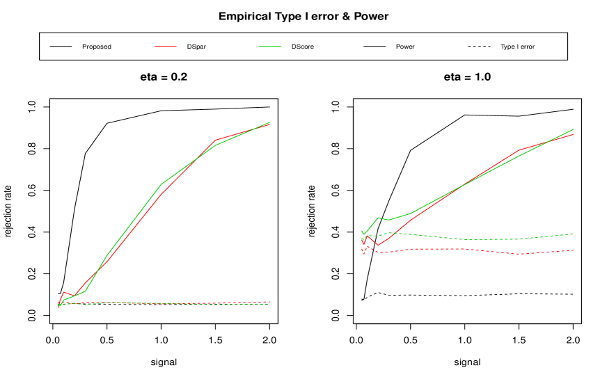
Figure 1: The average Type I errors and Powers with varying magnitude of the nonzero coefficients of $\bm{\Theta}$. The black, red and green lines represent the proposed approach, DSpar and DScore, respectively. The solid lines depict the averaged Powers while the dashed lines represent the averaged Type I errors.

Testing on $\bm{B}$:

We proceed to evaluate the empirical performance of our proposed method for testing the hypothesis $H_{0,B_{j}}:\bm{B}_{j}=\bm{\mathrm{0}}$ versus $H_{1,B_{j}}:\bm{B}_{j}\neq\bm{\mathrm{0}}$. We adopt the same data generating process as described in the beginning except that we set $\bm{B}_{j}=\bm{\mathrm{0}}$ for each $j\in\{1,\dotso,b_{m}\}$. Here $b_{m}$ controls the number of zero columns of $\bm{B}$ and is chosen from $\{5,10\}$. We also consider $p=50$, $\eta=0.1$ and vary $m$ within $\{20,50,100\}$. Similarly, we calculate the empirical Type I error and the empirical Power as

$$\text{Type I error}=\frac{1}{b_{m}}\sum_{j=1}^{b_{m}}1\left\{\textrm{Reject the null $H_{0,B_{j}}$}\right\},$$ (41)

$$\text{Power}=\frac{1}{(m-b_{m})}\sum_{j=b_{m}+1}^{m}1\left\{\textrm{Reject the null $H_{0,B_{j}}$}\right\}.$$

We repeat 100 times for each scenario. Table 2 contains the averaged Type I errors and Powers of our procedure in all settings. The Type I errors are not far from the nominal level 0.05 and get closer to it as $m$ increases while the Powers are close to one in all settings. These findings are in line of our Theorem 5.

Table 2: The averaged Type I errors and Powers at significance level 0.05 for the proposed method of testing $H_{0,B_{j}}:\bm{B}_{j}=\bm{\mathrm{0}}$ versus $H_{1,B_{j}}:\bm{B}_{j}\neq\bm{\mathrm{0}}$.

Metric	$b_{m}=5$			$b_{m}=10$
	$m=20$	$m=50$	$m=100$	$m=20$	$m=50$	$m=100$
Type I error	0.072	0.064	0.062	0.063	0.041	0.058
Power	0.989	1.000	0.998	1.000	0.988	0.999

6 Analysis on the stock mouse dataset

In this section, we validate our method on the heterogenous stock mouse dataset (Valdar et al., 2006) from Wellcome Trust Centre for Human Genetics. This dataset contains $129$ continuous phenotypes that can be categorized into six categories: Behavior, Diabetes, Ashma, Immunology, Haemotology and Biochemistry. The dataset also contains around $10,000$ Single Nucleotide Polymorphisms (SNPs) for each mouse. One primary interest is to discover significant associations between the SNPs and the phenotypes. Since both phenotypes and genotypes are measured by different experimenters at different time points and the mice are from different generations and families (Valdar et al., 2006), we expect the existence of unknown hidden effects, such as batch effects. We thus deploy our proposed method for finding significant entries of $\bm{\Theta}$ by adjusting the potential hidden effects.

To preprocess the data, since the measured phenotypes and SNPs vary for different groups of mice, we only consider the mice that should have all phenotypes measured. Meanwhile, we only keep the SNPs that have been measured by these retained mice. Finally, since there exists different levels of missingness among the phenotypes, we remove those phenotypes with percentage of missing values greater than $5\%$ and impute the missing values of the remaining phenotypes by using the average of their $20$-nearest neighbors. After the data preprocessing, we obtain a data set that has $n=810$ mice, $p=10,346$ measured SNPs and $m=104$ recorded phenotypes.

To deploy our method, we first use the procedure in Section 5.1 to find $\widehat{K}=28$ for this dataset and then apply our procedure in (3.3) to test the significance of each entry of $\bm{\Theta}$. The tuning parameters are chosen in the way as described in Section 5.2. To account for multiple testing problem, we apply the Bonferroni correction at 0.05 significant level. For comparison, we also run both DSpar and DScore (see, Section 5.3) with the same correction. To interpret and validate the discovered significant associations, we map the SNPs to either annotated genes or intergenic regions.

On the one hand, our approach and the other two methods detect some common meaningful signals. For example, in Diabetes related phenotypes, such as Insulin, both our method and DSpar find the SNP rs4213255 to be significant. This SNP is mapped to gene repro33 which has been shown to be associated with endocrine and exocrine glands (Goldfine et al., 1997) that directly mediates insulin level. Another SNP that is found by both our method and DSpar to be significant for an immunology phenotype is rs13476136 whose corresponding gene Tli1 (T lymphoma induced 1) has been demonstrated to directly affect immunology (Wielowieyski et al., 1999; Blake et al., 2003; Smith et al., 2019; Krupke et al., 2017). Furthermore, significance of the SNP rs3713052 is discovered for a Haemotology related phenotype (Haem.LICabs) by all three methods, and this SNP is mapped into the intergenic region between the gene Gm39049 and the gene Tenm4. Although the function of this intergenic region is unclear to us, the Tenm4 gene has been found to associate with the hematopoietic system (Blake et al., 2003; Smith et al., 2019; Krupke et al., 2017).

On the other hand, there exist many meaningful associations that are only identified to be significant by our method. For instance, the SNP rs6290322 is only found to be significant by our method for a Diabetes related phenotype (Glucose). It has been shown that the mapped gene gro57 of this SNP is associated with several Diabetic phenotypes (Blake et al., 2003; Smith et al., 2019; Krupke et al., 2017). Our method also finds the SNP rs3141314 to be significant for a Haemotology phenotype (Haem.PLT, platelet count). This SNP is mapped to gene hlb258 which is known to be functional related with the blood phenotypes (Blake et al., 2003; Smith et al., 2019; Krupke et al., 2017). In addition, several SNPs such as $rs3711203$ and $rs3725230$ are only found by our method to be significant for multiple immunological phenotypes. These SNPs are all mapped to gene slck (slick hair gene) which directly effects the integumentary system (Blake et al., 2003; Smith et al., 2019; Krupke et al., 2017). The integumentary system including the skin and corresponding appendages acts as a physical barrier between outside environment and internal environment hence plays an important role in the immune system.

Overall, our method finds more meaningful and significant SNPs than the other two methods. Specifically, for each method, we record the numbers of significant SNPs for each phenotype and report the summary statistics of these numbers in Table 3. We also run our testing procedure in Section 3.4 for $\bm{B}$ and all the test statistics are very large ($>427$ for all phenotypes), suggesting the existence of strong hidden effects. Although DSpar and Dscore are able to detect a few signals that are sufficiently large without adjusting the hidden effects, to find more weak/moderate yet meaningful signals, our proposed approach appears to be more effective.

Table 3: Summary statistics of the numbers of significant SNPs over all phenotypes by using different methods.

Method	Min	Mean	Median	Max
Ours	7	21.77	21	43
DSpar	0	1.77	0	39
DScore	0	0.09	0	5

Appendix A Column-wise $\ell_{2}$ convergence rates of $X\widehat{F}-XF$

We first provide theoretical guarantees of $\bm{X}\widehat{\bm{F}}-\bm{X}\bm{F}$ under the fixed design matrix $\bm{X}$ as the analysis is still valid for random design by first conditioning on $\bm{X}$. Recall from model (1) that $W$ is uncorrelated with $X$. To simplify the analysis under the fixed design scenario, we assume the independence between $X$ and $W$ in order to derive the deviation bounds of their cross product. We expect that the same theoretical guarantees hold under $\text{Cov}(X,W)=0$ by using more complicated arguments.

Recall that $\widehat{\bm{F}}=(\widehat{\bm{F}}_{1},\ldots,\widehat{\bm{F}}_{m})$ with $\widehat{\bm{F}}_{j}$ obtained from solving (14) for $1\leq j\leq m$. The following lemma characterizes the solution $\widehat{\bm{F}}_{j}=\widehat{\bm{\theta}}^{(j)}+\widehat{\bm{\delta}}^{(j)}$. It is proved in Chernozhukov et al. (2017).

Lemma 2.

For any $1\leq j\leq m$, let $(\widehat{\bm{\theta}}^{(j)},\widehat{\bm{\delta}}^{(j)})$ be any solution of (14), and denote

$$P_{\lambda_{2}^{(j)}}=\bm{X}\left(\bm{X}^{T}\bm{X}+n\lambda_{2}^{(j)}{\bm{I}}_{p}\right)^{-1}\bm{X}^{T},\qquad Q_{\lambda_{2}^{(j)}}={\bm{I}}_{n}-P_{\lambda_{2}^{(j)}}.$$ (42)

for any $\lambda_{2}^{(j)}\geq 0$ such that $P_{\lambda_{2}^{(j)}}$ exists. Then $\widehat{\bm{\theta}}^{(j)}$ is the solution of the following problem

$$\widehat{\bm{\theta}}^{(j)}=\arg\min_{\bm{\theta}\in\mathbb{R}^{p}}{1\over n}\left\|Q_{\lambda_{2}^{(j)}}^{1/2}(\bm{Y}_{j}-\bm{X}\bm{\theta})\right\|_{2}^{2}+\lambda_{1}^{(j)}\|\bm{\theta}\|_{1},$$ (43)

and $\widehat{\bm{\delta}}^{(j)}=(\bm{X}^{T}\bm{X}+n\lambda_{2}^{(j)}{\bm{I}}_{p})^{-1}\bm{X}^{T}(\bm{Y}_{j}-\bm{X}\widehat{\bm{\theta}}^{(j)})$, where $Q_{\lambda_{2}^{(j)}}^{1/2}$ is the principal matrix square root of $Q_{\lambda_{2}}$. Moreover, we have

$$\bm{X}\widehat{\bm{F}}_{j}=\bm{X}\left(\widehat{\bm{\theta}}^{(j)}+\widehat{\bm{\delta}}^{(j)}\right)=P_{\lambda_{2}^{(j)}}\bm{Y}_{j}+Q_{\lambda_{2}^{(j)}}\bm{X}\widehat{\bm{\theta}}^{(j)}.$$ (44)

To analyze $\widehat{\bm{F}}_{j}$, we first introduce the Restricted Eigenvalue (RE) (Bickel et al., 2009). For some given constant $\alpha\geq 1$ and integer $1\leq s\leq p$, define

$$\kappa(s,\alpha)=\min_{S\subseteq[p],|S|\leq s}~{}\min_{\Delta\in\mathcal{C}(S,\alpha)}{\|\bm{X}\Delta\|_{2}\over\sqrt{n}\|\Delta_{S\cdot}\|_{2}},$$ (45)

where $\mathcal{C}(S,\alpha):=\{\Delta\in\mathbb{R}^{p}\setminus\{\bm{\mathrm{0}}\}:\alpha\|\Delta_{S}\|_{1}\geq\|\Delta_{S^{c}}\|_{1}\}$. For $1\leq j\leq m$ and the $j$th response regression, define

$$\sigma_{j}^{2}=\gamma_{w}^{2}\bm{B}_{j}^{T}\Sigma_{W}\bm{B}_{j}+\gamma_{e}^{2}\sigma_{E_{j}}^{2}$$ (46)

where $\gamma_{w}$ and $\gamma_{e}$ are the sub-Gaussian constants defined in Assumption 1 and $\sigma_{E_{j}}^{2}=[\Sigma_{E}]_{jj}$. Write $M^{(j)}=n^{-1}\bm{X}^{T}Q_{\lambda_{2}^{(j)}}^{2}\bm{X}$ with $Q_{\lambda_{2}^{(j)}}$ defined in (42). Recall that $\widehat{\Sigma}=n^{-1}\bm{X}^{T}\bm{X}$ and its eigenvalue are $\Lambda_{1}\geq\Lambda_{2}\geq\cdots\geq\Lambda_{q}>0$ with $q=\textrm{rank}(\bm{X})$. Further recall $s_{n}$ is defined in (13). The following theorem provides the $\ell_{2}$ convergence rate of $\bm{X}\widehat{\bm{F}}_{j}-\bm{X}\bm{F}_{j}$ uniformly over $1\leq j\leq m$.

Theorem 6.

Under Assumptions 1, assume $\kappa(s_{n},4)>0$ and choose

$$\lambda_{1}^{(j)}=4\sigma_{j}\sqrt{6\max_{1\leq i\leq p}M_{ii}^{(j)}}\sqrt{\log(p\vee m)\over n}$$ (47)

and any $\lambda_{2}^{(j)}\geq 0$ in (14) such that $P_{\lambda_{2}^{(j)}}$ exists. With probability $1-2(p\vee m)^{-1}-m^{-1}$,

$${1\over n}\left\|\bm{X}\widehat{\bm{F}}_{j}-\bm{X}\bm{F}_{j}\right\|_{2}^{2} \lesssim\inf_{\begin{subarray}{c}(\bm{\theta}_{0},\bm{\delta}_{0}):\\ \bm{\theta}_{0}+\bm{\delta}_{0}=\bm{F}_{j}\end{subarray}}\Bigl{[}Rem_{1,j}+Rem_{2,j}(\bm{\delta}_{0})+Rem_{3,j}(\bm{\theta}_{0})\Bigr{]}$$

holds uniformly over $1\leq j\leq m$, where

$$Rem_{1,j}=\left({\rm tr}\left(P_{\lambda_{2}^{(j)}}^{2}\right)+\left\|P_{\lambda_{2}^{(j)}}^{2}\right\|_{{\rm op}}\log m\right){\sigma_{j}^{2}\over n}$$

$$Rem_{2,j}(\bm{\delta}_{0})=\lambda_{2}^{(j)}~{}\bm{\delta}_{0}^{T}\widehat{\Sigma}(\widehat{\Sigma}+\lambda_{2}^{(j)}{\bm{I}}_{p})^{-1}\bm{\delta}_{0}$$

$$Rem_{3,j}(\bm{\theta}_{0})={\lambda_{2}^{(j)}(\Lambda_{1}+\lambda_{2}^{(j)})\over(\Lambda_{q}+\lambda_{2}^{(j)})^{2}}\left(\max_{1\leq i\leq p}\widehat{\Sigma}_{ii}\right){s_{0}\log(p\vee m)\over\kappa^{2}(s_{n},4)}{\sigma_{j}^{2}\over n}.$$

Proof.

Theorem 6 can be proved by using the line of arguments in the proof of Theorem 4 in Bing et al. (2020) except for working on the following event

$$\mathcal{E}:=\bigcap_{i=1}^{p}\bigcap_{j=1}^{m}\left\{\left|\bm{X}_{i}^{T}Q_{\lambda_{2}^{(j)}}\bm{\epsilon}_{j}\right|\leq{n\over 4}\lambda_{1}^{(j)}\right\}$$ (48)

with $\lambda_{1}^{(j)}$ defined in (47). To establish $\mathbb{P}(\mathcal{E})$, pick any $1\leq i\leq p$ and $1\leq j\leq m$. We first note that, by the independence of $\bm{\epsilon}_{tj}$ for $1\leq t\leq n$, $\bm{\epsilon}_{j}^{T}Q_{\lambda_{2}^{(j)}}\bm{X}_{i}$ is sub-Gaussian with sub-Gaussian parameter

$$\sigma_{j}\sqrt{\bm{X}_{i}^{T}Q_{\lambda_{2}^{(j)}}^{2}\bm{X}_{i}}=\sigma_{j}\sqrt{nM_{ii}^{(j)}}.$$

Thus, the basic tail inequality of sub-Gaussian random variable yields

$$\mathbb{P}\left\{\left|\bm{X}_{i}^{T}Q_{\lambda_{2}^{(j)}}\bm{\epsilon}_{j}\right|>t\sigma_{j}\sqrt{nM_{ii}^{(j)}}\right\}\leq 2e^{-t^{2}/2},\quad\text{for all }t\geq 0.$$

Choose $t=\sqrt{6\log(p\vee m)}$ and take the union bounds over $1\leq i\leq p$ and $1\leq j\leq m$ to obtain $\mathbb{P}(\mathcal{E})\geq 1-2(p\wedge m)^{-1}.$ ∎

We remark that Theorem 6 in particular holds for the true $\bm{\theta}_{j}=\bm{\Theta}_{j}$ and $\bm{\delta}_{j}=\bm{A}\bm{B}_{j}$, for $1\leq j\leq m$, whenever they are identifiable.

Appendix B Main proofs

B.1 Proof of Theorem 1: identifiability

From model (5) and noting that $\text{Cov}(X,\epsilon)=\bm{\mathrm{0}}$, $\bm{\Theta}+\bm{A}\bm{B}$ can be identified from $[\text{Cov}(X)]^{-1}\text{Cov}(X,Y)$, and so is $\Sigma_{\epsilon}$. Let $\bm{U}_{K}\in\mathbb{R}^{m\times K}$ denote the first $K$ eigenvectors of $\Sigma_{\epsilon}$. An application of the Davis Kahan Theorem yields

$$\|\bm{U}_{K}\bm{U}_{K}^{T}-P_{B}\|_{{\rm op}}\leq{\sqrt{2}\|\Sigma_{E}\|_{{\rm op}}\over\lambda_{K}(\bm{B}^{T}\Sigma_{W}\bm{B})}=o(1)$$

under condition (8). Thus, $P_{B}^{\perp}$ is recovered asymptotically and so is $\bm{\Theta}P_{B}^{\perp}=(\bm{\Theta}+\bm{A}\bm{B})P_{B}^{\perp}$. Finally, for each $1\leq i\leq p$ and $1\leq j\leq m$, since under condition (11),

$$|\bm{\Theta}_{i\cdot}^{T}P_{B}\bm{e}_{j}|={} \left|\bm{\Theta}_{i\cdot}^{T}\bm{B}^{T}\Sigma_{W}^{1/2}\left(\Sigma_{W}^{1/2}\bm{B}\bm{B}^{T}\Sigma_{W}^{1/2}\right)^{-1}\Sigma_{W}^{1/2}\bm{B}\bm{e}_{j}\right|$$ (49)

$$\leq{} \|\bm{\Theta}_{i\cdot}\|_{1}\left\|\bm{B}^{T}\Sigma_{W}^{1/2}\left(\Sigma_{W}^{1/2}\bm{B}\bm{B}^{T}\Sigma_{W}^{1/2}\right)^{-1}\right\|_{\infty,2}\left\|\Sigma_{W}^{1/2}\bm{B}\bm{e}_{j}\right\|_{2}$$

$$\leq{} \|\bm{\Theta}_{i\cdot}\|_{1}\max_{1\leq\ell\leq m}\|\Sigma_{W}^{1/2}\bm{B}_{\ell}\|_{2}[\lambda_{K}(\bm{B}^{T}\Sigma_{W}\bm{B})]^{-1}\|\Sigma_{W}^{1/2}\bm{B}_{j}\|_{2}$$

$$={} \mathcal{O}\left({\|\bm{\Theta}_{i\cdot}\|_{1}\over m}\right),$$

we conclude that

$$\bm{\Theta}_{ij}=[\bm{\Theta}P_{B}^{\perp}]_{ij}+[\bm{\Theta}P_{B}]_{ij}=[\bm{\Theta}P_{B}^{\perp}]_{ij}+o(1).$$

This completes the proof. ∎

B.2 Proof of Theorem 4: The uniform convergence rate of $\widehat{B}_{j}$

Recall from (16) that

$${1\over nm}\widehat{\bm{\epsilon}}^{T}\widehat{\bm{\epsilon}}=\bm{V}\bm{D}^{2}\bm{V}^{T}.$$

We work on the intersection of the events

$$\mathcal{E}_{F} :=\left\{\max_{1\leq j\leq m}{1\over n}\|\bm{X}\widehat{\bm{F}}_{j}-\bm{X}\bm{F}_{j}\|_{2}^{2}\lesssim r_{n}\right\},$$ (50)

$$\mathcal{E}_{D} :=\left\{\sqrt{c_{W}c_{B}}\lesssim\lambda_{K}(\bm{D}_{K})\leq\lambda_{1}(\bm{D}_{K})\lesssim\sqrt{C_{W}C_{B}}\right\},$$ (51)

with $r_{n}$ defined in Assumption 4 and $c_{B},C_{B},c_{W},C_{W}$ defined in Assumption 2. Lemma 5 and Assumption 4 guarantee that $\lim_{n\to\infty}\mathbb{P}(\mathcal{E}_{F}\cap\mathcal{E}_{D})=1$.

By (17), observe that

$${1\over nm}\widehat{\bm{\epsilon}}^{T}\widehat{\bm{\epsilon}}\widehat{\bm{B}}^{T}=\bm{V}\bm{D}^{2}\bm{V}^{T}\sqrt{m}\bm{V}_{K}\bm{D}_{K}=\widehat{\bm{B}}^{T}\bm{D}_{K}^{2}.$$

Plugging

$$\widehat{\bm{\epsilon}}=\bm{Y}-\bm{X}\widehat{\bm{F}}=\bm{\epsilon}+\underbrace{\bm{X}\bm{F}-\bm{X}\widehat{\bm{F}}}_{\bm{\Delta}}$$ (52)

into the above display yields

$${1\over nm}\left(\bm{\epsilon}^{T}\bm{\epsilon}+\bm{\epsilon}^{T}\bm{\Delta}+\bm{\Delta}^{T}\bm{\epsilon}+\bm{\Delta}^{T}\bm{\Delta}\right)\widehat{\bm{B}}^{T}\bm{D}_{K}^{-2}=\widehat{\bm{B}}^{T}.$$

Since

$${1\over nm}\bm{\epsilon}^{T}\bm{\epsilon}={1\over nm}\left(\bm{B}^{T}\bm{W}^{T}\bm{W}\bm{B}+\bm{B}^{T}\bm{W}^{T}\bm{E}+\bm{E}^{T}\bm{W}\bm{B}+\bm{E}^{T}\bm{E}\right),$$

using the definition in (34) gives

$$\widehat{\bm{B}}^{T}-\bm{B}^{T}\bm{H}_{0}^{T}$$

$$={1\over nm}\left(\bm{B}^{T}\bm{W}^{T}\bm{E}+\bm{E}^{T}\bm{W}\bm{B}+\bm{E}^{T}\bm{E}+\bm{\epsilon}^{T}\bm{\Delta}+\bm{\Delta}^{T}\bm{\epsilon}+\bm{\Delta}^{T}\bm{\Delta}\right)\widehat{\bm{B}}^{T}\bm{D}_{K}^{-2}$$ (53)

$$={1\over n\sqrt{m}}\left(\bm{B}^{T}\bm{W}^{T}\bm{E}+\bm{E}^{T}\bm{W}\bm{B}+\bm{E}^{T}\bm{E}+\bm{\epsilon}^{T}\bm{\Delta}+\bm{\Delta}^{T}\bm{\epsilon}+\bm{\Delta}^{T}\bm{\Delta}\right)\bm{V}_{K}\bm{D}_{K}^{-1},$$

where we used (17) in the last step. Pick any $1\leq j\leq m$ and multiply both sides of the above display by $\bm{e}_{j}$. We proceed to bound each corresponding terms on the right hand side.

First, invoking Lemma 6 and $\mathcal{E}_{D}$ gives

$$\left\|\bm{e}_{j}^{T}\bm{B}^{T}\bm{W}^{T}\bm{E}\bm{V}_{K}\bm{D}_{K}^{-1}\right\|_{2}\lesssim\|\bm{B}_{j}^{T}\bm{W}^{T}\bm{E}\|_{2}\lesssim\sqrt{nm\log m}$$

with probability at least $1-8m^{-1}$. Similarly, we obtain

$${1\over n\sqrt{m}}\left\|\bm{e}_{j}^{T}\left(\bm{B}^{T}\bm{W}^{T}\bm{E}+\bm{E}^{T}\bm{W}\bm{B}+\bm{E}^{T}\bm{E}\right)\bm{V}_{K}\bm{D}_{K}^{-1}\right\|_{2}\lesssim\sqrt{\log m\over n\wedge m}.$$

On the other hand, Lemma 7 together with Assumption 4 ensures that, with probability $1-8m^{-1}$,

$${1\over n\sqrt{m}}\left\|\bm{e}_{j}^{T}\left(\bm{\epsilon}^{T}\bm{\Delta}+\bm{\Delta}^{T}\bm{\epsilon}+\bm{\Delta}^{T}\bm{\Delta}\right)\bm{V}_{K}\bm{D}_{K}^{-1}\right\|_{2}$$ (54)

$$\lesssim~{}\sqrt{r_{n}}\sqrt{Rem_{1,j}+Rem_{2,j}(\bm{\delta}_{j})+Rem_{3,j}(\bm{\theta}_{j})}+r_{n,1}+\sqrt{r_{n,2}\log(m)\over n}+r_{n,3}\sqrt{1\over n}$$

$$\lesssim~{}r_{n}$$

uniformly over $1\leq j\leq m$. Here, for convenience, we write

$$r_{n,1}=\max_{1\leq j\leq m}Rem_{1,j},\quad r_{n,2}=\max_{1\leq j\leq m}Rem_{2,j}(\bm{\delta}_{j}),\quad r_{n,3}=\max_{1\leq j\leq m}Rem_{3,j}(\bm{\theta}_{j}).$$ (55)

Collecting the previous three displays concludes the desired rate. The proof is completed by noting that $m=m(n)\to\infty$ whence the probabilities tend to one as $n\to\infty$. ∎

B.3 Proof of Lemma 1: $\ell_{1}$ convergence rate of the initial estimator $\widehat{\Theta}_{1}$

Recall $\widehat{\Sigma}=n^{-1}\bm{X}^{T}\bm{X}$ and $\kappa(s_{n},4)$ is defined in (45). Define the following event

$$\mathcal{E}_{\bm{X}}:=\left\{\kappa(s_{n},4)\geq c,~{}\max_{1\leq j\leq p}\widehat{\Sigma}_{jj}\leq C,~{}{1\over\sqrt{n}}\|\bm{X}\bm{\Theta}\|_{2,1}\leq C^{\prime}M_{n}\sqrt{s_{n}},~{}{1\over\sqrt{n}}\|\bm{X}\bm{A}\|_{{\rm op}}\leq C^{\prime}\right\}$$ (56)

for some finite constants $C\geq c>0$ and $C^{\prime}>0$. Lemma 10 in Appendix C.2 proves that $\lim_{n\to\infty}\mathbb{P}(\mathcal{E}_{\bm{X}})=1$ under the conditions of Theorem 1. Recall $r_{n}$ from Assumption 4. Define

$$\eta_{n}=\sqrt{\log m\over n\wedge m}+r_{n}.$$ (57)

Further recall $\widetilde{\bm{B}}$ and $\bm{H}_{0}$ are defined in (35) and (34). We work on the event

$$\mathcal{E}_{\bm{X}}\cap\left\{\|(\widetilde{\bm{B}}-\widehat{\bm{B}})\widehat{P}_{B}^{\perp}\bm{e}_{1}\|_{2}\lesssim\eta_{n}\right\}\cap\left\{\|(\widehat{P}_{B}-P_{B})\bm{e}_{1}\|_{\infty}\lesssim{\eta_{n}\over m}\right\}\cap\left\{\lambda_{K}(\bm{H}_{0})\gtrsim c_{H}\right\}$$ (58)

which, according to Lemmas 10, 8 and 9, holds with probability tending to one.

Recall that $\bar{\bm{\Theta}}_{1}=\bm{\Theta}P_{B}^{\perp}\bm{e}_{1}$. Starting with

$$\frac{1}{n}\big{\|}\widetilde{\bm{y}}-\bm{X}\widehat{\bm{\Theta}}_{1}\big{\|}_{2}^{2}+\lambda_{3}\|\widehat{\bm{\Theta}}_{1}\|_{1}\leq\frac{1}{n}\big{\|}\widetilde{\bm{y}}-\bm{X}\bar{\bm{\Theta}}_{1}\big{\|}_{2}^{2}+\lambda_{3}\|\bar{\bm{\Theta}}_{1}\|_{1},$$

work out the squares to obtain

$${1\over n}\left\|\bm{X}(\widehat{\bm{\Theta}}_{1}-\bar{\bm{\Theta}}_{1})\right\|_{2}^{2}\leq{2\over n}\left|\langle\bm{X}(\widehat{\bm{\Theta}}_{1}-\bar{\bm{\Theta}}_{1}),\widetilde{\bm{y}}-\bm{X}\bar{\bm{\Theta}}_{1}\right|+\lambda_{3}\|\bar{\bm{\Theta}}_{1}\|_{1}-\lambda_{3}\|\widehat{\bm{\Theta}}_{1}\|_{1}.$$

By noting that

$$\widetilde{\bm{y}}-\bm{X}\bar{\bm{\Theta}}_{1} =\left[\bm{X}(\bm{\Theta}+\bm{A}\bm{B})+\bm{W}\bm{B}+\bm{E}\right]\widehat{P}_{B}^{\perp}\bm{e}_{1}-\bm{X}\bm{\Theta}P_{B}^{\perp}\bm{e}_{1}$$

$$=\bm{X}\bm{A}\bm{B}\widehat{P}_{B}^{\perp}\bm{e}_{1}+\bm{W}\bm{B}\widehat{P}_{B}^{\perp}\bm{e}_{1}+\bm{E}\widehat{P}_{B}^{\perp}\bm{e}_{1}+\bm{X}\bm{\Theta}(\widehat{P}_{B}^{\perp}-P_{B}^{\perp})\bm{e}_{1}$$

and by writing $\bm{\Delta}=\widehat{\bm{\Theta}}_{1}-\bar{\bm{\Theta}}_{1}$, we have

$${2\over n}\left|\langle\bm{X}\bm{\Delta},\widetilde{\bm{y}}-\bm{X}\bar{\bm{\Theta}}_{1}\right| \leq{2\over n}\left|\bm{e}_{1}^{T}\widehat{P}_{B}^{\perp}\bm{E}^{T}\bm{X}\bm{\Delta}\right|+{2\over n}\left\|\bm{X}\bm{\Delta}\right\|_{2}Rem$$

$$\leq{2\over n}\left\|\bm{e}_{1}^{T}\widehat{P}_{B}^{\perp}\bm{E}^{T}\bm{X}\right\|_{\infty}\|\bm{\Delta}\|_{1}+{2\over n}\left\|\bm{X}\bm{\Delta}\right\|_{2}Rem.$$

where

$$Rem={1\over\sqrt{n}}\left\|\bm{X}\bm{A}\bm{B}\widehat{P}_{B}^{\perp}\bm{e}_{1}+\bm{W}\bm{B}\widehat{P}_{B}^{\perp}\bm{e}_{1}+\bm{X}\bm{\Theta}(P_{B}-\widehat{P}_{B})\bm{e}_{1}\right\|_{2}.$$

Provided that

$$\left\|\bm{e}_{1}^{T}\widehat{P}_{B}^{\perp}\bm{E}^{T}\bm{X}\right\|_{\infty}\leq{n\over 4}\lambda_{3},$$ (59)

from the fact that $\|\bar{\bm{\Theta}}_{1}\|_{0}\leq s_{n}$, using $\|\bar{\bm{\Theta}}_{1}\|_{1}-\|\widehat{\bm{\Theta}}_{1}\|_{1}\leq\|\bm{\Delta}_{S}\|_{1}+\|\bm{\Delta}_{S^{c}}\|_{1}$ with $S:=\mathrm{supp}(\bar{\bm{\Theta}}_{1})$ and $|S|\leq s_{n}$ gives

$${1\over n}\left\|\bm{X}\bm{\Delta}\right\|_{2}^{2}\leq{2\over n}\left\|\bm{X}\bm{\Delta}\right\|_{2}Rem+{3\over 2}\lambda_{3}\|\bm{\Delta}_{S}\|_{1}-{1\over 2}\lambda_{3}\|\bm{\Delta}_{S^{c}}\|_{1}.$$

We now bound from above $Rem$. By recalling that $\widetilde{\bm{B}}=\bm{H}_{0}\bm{B}$,

$${1\over\sqrt{n}}\left\|\bm{X}\bm{A}\bm{B}\widehat{P}_{B}^{\perp}\bm{e}_{1}\right\|_{2} ={1\over\sqrt{n}}\left\|\bm{X}\bm{A}\bm{H}_{0}^{-1}(\widetilde{\bm{B}}-\widehat{\bm{B}})\widehat{P}_{B}^{\perp}\bm{e}_{1}\right\|_{2}$$

$$\leq{1\over\sqrt{n}}\left\|\bm{X}\bm{A}\bm{H}_{0}^{-1}\right\|_{{\rm op}}\left\|(\widetilde{\bm{B}}-\widehat{\bm{B}})\widehat{P}_{B}^{\perp}\bm{e}_{1}\right\|_{2}$$

$$\lesssim{1\over\sqrt{n}}\left\|\bm{X}\bm{A}\right\|_{{\rm op}}\eta_{n} \textrm{by }(\ref{def_event_misc})$$

$$\lesssim\eta_{n} \textrm{by }(\ref{def_event_X}).$$

By (58), we also have

$${1\over\sqrt{n}}\left\|\bm{X}\bm{\Theta}(\widehat{P}_{B}-P_{B})\bm{e}_{1}\right\|_{2} \leq{1\over\sqrt{n}}\left\|\bm{X}\bm{\Theta}\right\|_{2,1}\left\|(\widehat{P}_{B}-P_{B})\bm{e}_{1}\right\|_{\infty}\lesssim{M_{n}\sqrt{s_{n}}\over m}\eta_{n}.$$

Together with Lemma 4, we also have

$${1\over\sqrt{n}}\left\|\bm{W}\bm{B}\widehat{P}_{B}^{\perp}\bm{e}_{1}\right\|_{2} \lesssim{1\over\sqrt{n}}\left\|\bm{W}\right\|_{{\rm op}}\left\|(\widetilde{\bm{B}}-\widehat{\bm{B}})\widehat{P}_{B}^{\perp}\bm{e}_{1}\right\|_{2}\lesssim\eta_{n}$$

with probability $1-2e^{-n}$. We thus conclude that with the same probability, on the event (58),

$$Rem\lesssim\eta_{n}\left(1+{M_{n}\sqrt{s_{n}}\over m}\right).$$

Following the same line of arguments as the proof of Theorem 6 in Bing et al. (2020), it is straightforward to show that, on the event (58) and for any $\lambda_{3}$ such that (59) holds,

$$\|\widehat{\bm{\Theta}}_{1}-\bar{\bm{\Theta}}_{1}\|_{1}\lesssim\max\left\{{\lambda_{3}},~{}{(\widetilde{\lambda}_{3})^{2}\over\lambda_{3}}\right\}{s_{n}\over\kappa^{2}(s_{n},4)},$$ (60)

holds with probability $1-2e^{-n}$, where

$$\widetilde{\lambda}_{3}=\eta_{n}\left(1+{M_{n}\sqrt{s_{n}}\over m}\right){\kappa(s_{n},4)\over\sqrt{s_{n}}}.$$ (61)

It remains to show (59) holds with probability tending to one for any

$$\lambda_{3}\geq\bar{\lambda}_{3}\asymp\sigma_{E_{1}}\sqrt{\max_{1\leq j\leq p}\widehat{\Sigma}_{jj}}\sqrt{\log p\over n}.$$ (62)

If this holds, then observe that (62), (60) and (61) readily imply

$$\|\widehat{\bm{\Theta}}_{1}-\bar{\bm{\Theta}}_{1}\|_{1} \lesssim(\bar{\lambda}_{3}\vee\widetilde{\lambda}_{3}){s_{n}\over\kappa^{2}(s_{n},4)}$$ (63)

$$\lesssim s_{n}\sqrt{\log p\over n}+\left(\sqrt{s_{n}}+{M_{n}s_{n}\over m}\right)\eta_{n}$$

by choosing $\lambda_{3}$ appropriately. The result immediately follows from (57).

To prove (59) holds for any $\lambda_{3}\geq\bar{\lambda}_{3}$, note that

$$\left\|\bm{e}_{1}^{T}\widehat{P}_{B}^{\perp}\bm{E}^{T}\bm{X}\right\|_{\infty} \leq\left\|\bm{e}_{1}^{T}\bm{E}^{T}\bm{X}\right\|_{\infty}+\left\|\bm{e}_{1}^{T}\widehat{P}_{B}\bm{E}^{T}\bm{X}\right\|_{\infty}$$

$$\leq\left\|\bm{e}_{1}^{T}\bm{E}^{T}\bm{X}\right\|_{\infty}+\left\|\bm{e}_{1}^{T}\widehat{P}_{B}\right\|_{2}\left\|\bm{E}^{T}\bm{X}\right\|_{2,\infty}.$$

Since $\bm{E}_{1}^{T}\bm{X}_{j}$ is $\gamma_{e}\sqrt{n\widehat{\Sigma}_{jj}[\Sigma_{E}]_{11}}$ sub-Gaussian, the sub-Gaussian tail probability together with union bounds over $1\leq j\leq p$ yields

$$\mathbb{P}\left\{\left\|\bm{e}_{1}^{T}\bm{E}^{T}\bm{X}\right\|_{\infty}\leq 2\gamma_{e}\sqrt{n\log p}\sqrt{[\Sigma_{E}]_{11}\max_{1\leq j\leq p}\widehat{\Sigma}_{jj}}\right\}\geq 1-2p^{-1}.$$

Furthermore, noting that

$$\left\|\bm{E}^{T}\bm{X}\right\|_{2,\infty}^{2}=\max_{1\leq j\leq p}\bm{X}_{j}^{T}\bm{E}\Sigma_{E}^{-1/2}\Sigma_{E}\Sigma_{E}^{-1/2}\bm{E}\bm{X}_{j}$$

and $\bm{X}_{j}\bm{E}\Sigma_{E}^{-1/2}$ is $\gamma_{e}\sqrt{n\widehat{\Sigma}_{jj}}$ sub-Gaussian, an application of Lemma 14 with union bounds over $1\leq j\leq p$ gives

$$\mathbb{P}\left\{\left\|\bm{E}^{T}\bm{X}\right\|_{2,\infty}^{2}\leq\gamma_{e}^{2}n\max_{1\leq j\leq p}\widehat{\Sigma}_{jj}\left(\sqrt{{\rm tr}(\Sigma_{E})}+\sqrt{4\|\Sigma_{E}\|_{{\rm op}}\log p}\right)^{2}\right\}\geq 1-p^{-1}.$$

By part (E) of Lemma 8, we conclude that

$$\mathbb{P}\left\{{1\over n}\left\|\bm{e}_{1}^{T}\widehat{P}_{B}^{\perp}\bm{E}^{T}\bm{X}\right\|_{\infty}\lesssim\gamma_{e}C_{E}\sqrt{\max_{1\leq j\leq p}\widehat{\Sigma}_{jj}}\sqrt{\log p\over n}\right\}\geq 1-3p^{-1}$$

where

$$C_{E}=\sqrt{[\Sigma_{E}]_{11}}+\sqrt{{\rm tr}(\Sigma_{E})\over m\log p}+\sqrt{\|\Sigma_{E}\|_{{\rm op}}\over m}\lesssim 1.$$

This completes the proof. ∎

B.4 Proof of Theorem 2: asymptotic normality of $\widetilde{\Theta}_{11}$

Recall that $\bar{\bm{\Theta}}_{1}=\bm{\Theta}P_{B}^{\perp}\bm{e}_{1}$ so that $\bar{\Theta}_{11}=\bm{e}_{1}^{T}\bm{\Theta}P_{B}^{\perp}\bm{e}_{1}$. By the definition of $\widetilde{\Theta}_{11}$ and $\bar{\Theta}_{11}$, we have

$$\widetilde{\Theta}_{11}-\bar{\Theta}_{11} =\widehat{\Theta}_{11}-\bar{\Theta}_{11}+\widehat{\bm{\omega}}_{1}^{T}\frac{1}{n}\bm{X}^{T}(\widetilde{\bm{y}}-\bm{X}\widehat{\bm{\Theta}}_{1})$$ (64)

$$=\underbrace{(\bm{e}_{1}-\frac{1}{n}\bm{X}^{T}\bm{X}\widehat{\bm{\omega}}_{1})^{T}(\widehat{\bm{\Theta}}_{1}-\bar{\bm{\Theta}}_{1})}_{I_{1}}+\widehat{\bm{\omega}}_{1}^{T}\frac{1}{n}\bm{X}^{T}(\widetilde{\bm{y}}_{1}-\bm{X}\bar{\bm{\Theta}}_{1})$$

$$=I_{1}+\widehat{\bm{\omega}}_{1}^{T}\frac{1}{n}\bm{X}^{T}\left[(\bm{X}(\bm{\Theta}+\bm{A}\bm{B})+\bm{W}\bm{B}+\bm{E})\widehat{P}_{B}^{\perp}\bm{e}_{1}-\bm{X}\bm{\Theta}P_{B}^{\perp}\bm{e}_{1}\right]$$

$$=I_{1}+\underbrace{\widehat{\bm{\omega}}_{1}^{T}\frac{1}{n}\bm{X}^{T}\bm{X}\bm{\Theta}(\widehat{P}_{B}^{\perp}-P_{B}^{\perp})\bm{e}_{1}}_{I_{2}}+\underbrace{\widehat{\bm{\omega}}_{1}^{T}\frac{1}{n}\bm{X}^{T}\bm{X}\bm{A}\bm{B}\widehat{P}_{B}^{\perp}\bm{e}_{1}}_{I_{3}}$$

$$~{}~{}~{}~{}~{}~{}~{}~{}~{}~{}~{}~{}~{}~{}~{}~{}~{}~{}+\underbrace{\widehat{\bm{\omega}}_{1}^{T}\frac{1}{n}\bm{X}^{T}\bm{W}\bm{B}\widehat{P}_{B}^{\perp}\bm{e}_{1}}_{I_{4}}+\underbrace{\widehat{\bm{\omega}}_{1}^{T}\frac{1}{n}\bm{X}^{T}\bm{E}\widehat{P}_{B}^{\perp}\bm{e}_{1}}_{I_{5}}$$

$$= I_{1}+I_{2}+I_{3}+I_{4}+I_{5}.$$

In what follows, we will characterize $I_{1}$ through $I_{5}$, respectively. For simplicity, define

$$\xi_{n}=s_{n}\sqrt{\log p\over n}+\left({s_{n}M_{n}\over m}+\sqrt{s_{n}}\right)\left(\sqrt{\log m\over n}+r_{n}\right)$$ (65)

such that $\|\widehat{\bm{\Theta}}_{1}-\bar{\bm{\Theta}}_{1}\|_{1}=\mathcal{O}_{\mathbb{P}}(\xi_{n})$ from Theorem 1.

• For $I_{1}$, the KKT condition of (20) implies that (van de Geer et al., 2014)

  $$\left\|\frac{1}{n}\bm{X}^{T}\bm{X}\widehat{\bm{\omega}}_{1}-\bm{e}_{1}\right\|_{\infty}\leq\frac{\widetilde{\lambda}}{2\widehat{\tau}_{1}^{2}},$$

  which, together with Lemma 11 and Theorem 1, yields

  $$|I_{1}|\leq\|\widehat{\bm{\Theta}}_{1}-\bar{\bm{\Theta}}_{1}\|_{1}\|\bm{e}_{1}-\frac{1}{n}\bm{X}^{T}\bm{X}\widehat{\bm{\omega}}\|_{\infty}=\mathcal{O}_{\mathbb{P}}\left(\xi_{n}\sqrt{\log p\over n}\right).$$ (66)

• For $I_{2}$, direct calculation gives us

  $$I_{2} =(\bm{e}_{1}-\frac{1}{n}\bm{X}^{T}\bm{X}\widehat{\bm{\omega}}_{1})^{T}\bm{\Theta}(P_{B}-\widehat{P}_{B})\bm{e}_{1}+\bm{\Theta}_{1\cdot}^{T}(P_{B}-\widehat{P}_{B})\bm{e}_{1}$$

  $$=I_{21}+I_{22}.$$

  Recall that $\eta_{n}$ is defined in (57). We have

  $$I_{21}\leq\|\bm{e}_{1}-\frac{1}{n}\bm{X}^{T}\bm{X}\widehat{\bm{\omega}}_{1}\|_{\infty}\|\bm{\Theta}\|_{1,1}\|(P_{B}-\widehat{P}_{B})\bm{e}_{1}\|_{\infty}=\mathcal{O}_{\mathbb{P}}\left(\frac{s_{n}M_{n}\eta_{n}}{m}\sqrt{\log p\over n}\right),$$

  where the last step follows from Lemma 9, Lemma 11 and $\|\bm{\Theta}\|_{1,1}\leq s_{n}\|\bm{\Theta}\|_{\infty,1}\leq s_{n}M_{n}$ from (13). Similarly, we can show that

  $$|I_{22}|\leq\|\bm{\Theta}_{1\cdot}\|_{1}\|(P_{B}-\widehat{P}_{B})\bm{e}_{1}\|_{\infty}=\mathcal{O}_{\mathbb{P}}\left(\frac{M_{n}\eta_{n}}{m}\right),$$

  and therefore

  $$|I_{2}|=\mathcal{O}_{\mathbb{P}}\left(\left(1+s_{n}\sqrt{\log p\over n}\right)\frac{M_{n}\eta_{n}}{m}\right)=\mathcal{O}_{\mathbb{P}}\left(\frac{M_{n}\eta_{n}}{m}\right).$$ (67)

• For $I_{3}$, recall from (34) and (35) that $\bm{A}\bm{B}=\widetilde{\bm{A}}\widetilde{\bm{B}}:=(\bm{A}\bm{H}_{0}^{-1})(\bm{H}_{0}\bm{B})$ on the event

  $$\mathcal{E}_{H}=\left\{c_{H}\lesssim\lambda_{K}(\bm{H}_{0})\leq\lambda_{1}(\bm{H}_{0})\lesssim C_{H}\right\}$$

  with $c_{H}$ and $C_{H}$ defined in Lemma 8. On the event $\mathcal{E}_{H}$, we obtain

  $$|I_{3}| =|\widehat{\bm{\omega}}_{1}^{T}\frac{1}{n}\bm{X}^{T}\bm{X}\widetilde{\bm{A}}\widetilde{\bm{B}}\widehat{P}_{B}^{\perp}\bm{e}_{1}|$$

  $$\leq\|\widehat{\bm{\omega}}_{1}^{T}\frac{1}{n}\bm{X}^{T}\bm{X}\widetilde{\bm{A}}\|_{2}\|(\widetilde{\bm{B}}-\widehat{\bm{B}})\widehat{P}_{B}^{\perp}\bm{e}_{1}\|_{2} \textrm{by }\widehat{\bm{B}}\widehat{P}_{B}^{\perp}=\bm{\mathrm{0}}$$

  $$\lesssim c_{H}^{-1}\|\widehat{\bm{\omega}}_{1}^{T}\frac{1}{n}\bm{X}^{T}\bm{X}\bm{A}\|_{2}\|(\widetilde{\bm{B}}-\widehat{\bm{B}})\widehat{P}_{B}^{\perp}\bm{e}_{1}\|_{2}.$$

  Notice that $\lim_{n\to\infty}\mathbb{P}(\mathcal{E}_{H})=1$ and $\|(\widetilde{\bm{B}}-\widehat{\bm{B}})\widehat{P}_{B}^{\perp}\bm{e}_{1}\|_{2}=\mathcal{O}_{\mathbb{P}}(\bar{\eta})$ from parts (A) and (D) of Lemma 8, respectively. We bound from above $\|\widehat{\bm{\omega}}_{1}^{T}\frac{1}{n}\bm{X}^{T}\bm{X}\bm{A}\|_{2}$ as

  $$\|\widehat{\bm{\omega}}_{1}^{T}\frac{1}{n}\bm{X}^{T}\bm{X}\bm{A}\|_{2} \leq\|(\bm{e}_{1}-\frac{1}{n}\bm{X}^{T}\bm{X}\widehat{\bm{\omega}}_{1})^{T}\bm{A}\|_{2}+\|\bm{A}_{1\cdot}\|_{2}$$

  $$=\mathcal{O}_{\mathbb{P}}\left(\sqrt{s_{\Omega}\log p\over n}\right)+\|\bm{A}_{1\cdot}\|_{2}$$

  where the last step uses Lemma 12. We thus conclude

  $$|I_{3}|=\mathcal{O}_{\mathbb{P}}\left(\eta_{n}\sqrt{s_{\Omega}\log p\over n}+\eta_{n}\|\bm{A}_{1\cdot}\|_{2}\right).$$ (68)

• For $I_{4}$, on the event $\mathcal{E}_{H}$ and by writing $\widetilde{\bm{W}}=\bm{W}\bm{H}_{0}^{-1}$,

  $$|I_{4}|\leq\|\widehat{\bm{\omega}}_{1}^{T}\frac{1}{n}\bm{X}^{T}\widetilde{\bm{W}}\|_{2}\|(\widetilde{\bm{B}}-\widehat{\bm{B}})\widehat{P}_{B}^{\perp}\bm{e}_{1}\|_{2}\lesssim c_{H}^{-1}\|\widehat{\bm{\omega}}_{1}^{T}\frac{1}{n}\bm{X}^{T}\bm{W}\|_{2}\mathcal{O}_{\mathbb{P}}(\eta_{n}).$$

  Note that, conditioning on $\bm{X}$, $\widehat{\bm{\omega}}_{1}^{T}\bm{X}^{T}\bm{W}\Sigma_{W}^{-1/2}\in\mathbb{R}^{K}$ is $\gamma_{w}\sqrt{\widehat{\bm{\omega}}_{1}^{T}\bm{X}^{T}\bm{X}\widehat{\bm{\omega}}_{1}}$ sub-Gaussian random vector. An application of Lemma 14 yields, for all $t>0$,

  $$\mathbb{P}\left\{\|\widehat{\bm{\omega}}_{1}^{T}\bm{X}^{T}\bm{W}\|_{2}^{2}>\gamma_{w}^{2}(\widehat{\bm{\omega}}_{1}^{T}\bm{X}^{T}\bm{X}\widehat{\bm{\omega}}_{1})\left(\sqrt{{\rm tr}(\Sigma_{W})}+\sqrt{2\|\Sigma_{W}\|_{{\rm op}}t}\right)^{2}\right\}\leq e^{-t}.$$

  Note that

  $${1\over n}\widehat{\bm{\omega}}_{1}^{T}\bm{X}^{T}\bm{X}\widehat{\bm{\omega}}_{1} \leq\Omega_{11}+\left|\widehat{\bm{\omega}}_{1}^{T}{1\over n}\bm{X}^{T}\bm{X}\widehat{\bm{\omega}}_{1}-\Omega_{11}\right|$$ (69)

  $$=\mathcal{O}_{\mathbb{P}}\left(\Omega_{11}+\sqrt{s_{\Omega}\log p\over n}\right)$$ by Lemma 11

  $$=\mathcal{O}_{\mathbb{P}}(\Omega_{11})$$

  by using $s_{\Omega}\log p=o(n)$ and $\Omega_{11}\geq\Sigma_{11}^{-1}\geq C^{-1}$ from Assumption 3. By also noting that

  $$\Omega_{11}\leq{1\over\lambda_{\min}(\Sigma)}=\mathcal{O}(1)$$ (70)

  from Assumption 3, from ${\rm tr}(\Sigma_{W})\leq K\|\Sigma_{W}\|_{{\rm op}}=\mathcal{O}(1)$ and (69), we conclude

  $$\left\|\widehat{\bm{\omega}}_{1}^{T}\frac{1}{n}\bm{X}^{T}\bm{W}\right\|_{2}=\mathcal{O}_{\mathbb{P}}\left(1/\sqrt{n}\right).$$

  Hence

  $$I_{4}=\mathcal{O}_{\mathbb{P}}\left(\eta_{n}\over\sqrt{n}\right).$$ (71)

• For $I_{5}$, by definition

  $$\widehat{\bm{\omega}}_{1}^{T}\frac{1}{n}\bm{X}^{T}\bm{E}\widehat{P}_{B}^{\perp}\bm{e}_{1}= \widehat{\bm{\omega}}_{1}^{T}\frac{1}{n}\bm{X}^{T}\bm{E}P_{B}^{\perp}\bm{e}_{1}+\widehat{\bm{\omega}}_{1}^{T}\frac{1}{n}\bm{X}^{T}\bm{E}(P_{B}-\widehat{P}_{B})\bm{e}_{1}$$

  $$:= I_{51}+I_{52}.$$

  It’s easy to see that $\bm{E}\widehat{P}_{B}^{\perp}\bm{e}_{1}\in\mathbb{R}^{n}$ is an i.i.d Gaussian vector with covariance matrix $V_{11}{\bm{I}}_{n}$ and independent of $\bm{X}$, where

  $$V_{11}:=\bm{e}_{1}^{T}P_{B}^{\perp}\Sigma_{E}P_{B}^{\perp}\bm{e}_{1}.$$

  This implies that

  $$\sqrt{n}I_{51}~{}\big{|}~{}\bm{X}\sim N\left(0,\widehat{\bm{\omega}}_{1}^{T}\frac{1}{n}\bm{X}^{T}\bm{X}\widehat{\bm{\omega}}_{1}~{}V_{11}\right).$$

  We further note that

  $$V_{11}=[\Sigma_{E}]_{11}-\bm{e}_{1}^{T}P_{B}\Sigma_{E}\bm{e}_{1}-\bm{e}_{1}^{T}P_{B}\Sigma_{E}P_{B}^{\perp}\bm{e}_{1}=[\Sigma_{E}]_{11}+\mathcal{O}(1/\sqrt{m})$$ (72)

  by using $\|P_{B}\bm{e}_{1}\|_{2}=\mathcal{O}(1/\sqrt{m})$ deduced from (49). Hence, also by (69) and (70),

  $$\sqrt{n}I_{51}=\zeta+o_{\mathbb{P}}(1)$$ (73)

  where

  $$\zeta|\bm{X}\sim N\left(0,\widehat{\bm{\omega}}_{1}^{T}\frac{1}{n}\bm{X}^{T}\bm{X}\widehat{\bm{\omega}}_{1}~{}[\Sigma_{E}]_{11}\right).$$ (74)

  For the second term, we know

  $$|I_{52}|\leq|\widehat{\bm{\omega}}_{1}^{T}\frac{1}{n}\bm{X}^{T}\bm{E}(P_{B}-\widehat{P}_{B})\bm{e}_{1}| \leq\frac{1}{n}\|\bm{E}^{T}\bm{X}\widehat{\bm{\omega}}_{1}\|_{2}\|(\widehat{P}_{B}-P_{B})\bm{e}_{1}\|_{2}.$$

  Using the same arguments of bounding $\|\widehat{\bm{\omega}}_{1}^{T}\bm{X}^{T}\bm{W}\|_{2}$ as above, one can establish that

  $$\mathbb{P}\left\{\|\widehat{\bm{\omega}}_{1}^{T}\bm{X}^{T}\bm{E}\|_{2}^{2}>\gamma_{e}^{2}(\widehat{\bm{\omega}}_{1}^{T}\bm{X}^{T}\bm{X}\widehat{\bm{\omega}}_{1})\left(\sqrt{{\rm tr}(\Sigma_{E})}+\sqrt{2\|\Sigma_{E}\|_{{\rm op}}t}\right)^{2}\right\}\leq e^{-t},\quad\forall t>0.$$

  Hence, by $\|\Sigma_{E}\|_{{\rm op}}=\mathcal{O}(1)$, (69) and (70),

  $$\|\widehat{\bm{\omega}}_{1}^{T}\frac{1}{n}\bm{X}^{T}\bm{E}\|_{2}=\mathcal{O}_{\mathbb{P}}\left(\sqrt{m\over n}\right).$$

  Finally, invoke Lemma 9 to obtain

  $$|I_{52}|=\mathcal{O}_{\mathbb{P}}\left(\eta_{n}\over\sqrt{n}\right).$$ (75)

Collecting (66), (67), (68), (71), (73) and (75) and using

$$\bar{\Theta}_{11}=\Theta_{11}-\bm{\Theta}_{1\cdot}^{T}P_{B}\bm{e}_{1}\overset{(\ref{bd_bias})}{=}\Theta_{11}+\mathcal{O}(M_{n}/m)$$

conclude

$$\sqrt{n}\left(\widetilde{\Theta}_{11}-\Theta_{11}\right) =\zeta+\Delta$$

where $\zeta$ satisfies (74) and

$$\Delta =\mathcal{O}_{\mathbb{P}}\left(\xi_{n}\sqrt{\log p}+\left({M_{n}\sqrt{n}\over m}+\sqrt{s_{\Omega}\log p}+\sqrt{n}\|\bm{A}_{1\cdot}\|_{2}+1\right)\eta_{n}\right)+\mathcal{O}\left({M_{n}\sqrt{n}\over m}\right)+o_{\mathbb{P}}(1).$$

By $M_{n}\sqrt{n}=o(m)$, (65) and (57), after a bit algebra, we conclude

$$\Delta =\mathcal{O}_{\mathbb{P}}\left({s_{n}\log p\over\sqrt{n}}+\left({s_{n}M_{n}\sqrt{\log p}\over m}+\sqrt{(s_{n}\vee s_{\Omega})\log p}+\sqrt{n}\|\bm{A}_{1\cdot}\|_{2}+1\right)\eta_{n}\right)+o_{\mathbb{P}}(1)$$

$$=\mathcal{O}_{\mathbb{P}}\left(\left(\sqrt{(s_{n}\vee s_{\Omega})\log p}+\sqrt{n}\|\bm{A}_{1\cdot}\|_{2}+1\right)\left(\sqrt{\log m\over n}+r_{n}\right)\right)+o_{\mathbb{P}}(1)$$

$$=\mathcal{O}_{\mathbb{P}}\left(\sqrt{(s_{n}\vee s_{\Omega})\log(p)\log(m)\over n}\right)$$

$$\quad+\mathcal{O}_{\mathbb{P}}\left(\|\bm{A}_{1\cdot}\|_{2}\sqrt{\log m}+\left(\sqrt{(s_{n}\vee s_{\Omega})\log p}+\sqrt{n}\|\bm{A}_{1\cdot}\|_{2}\right)r_{n}\right)+o_{\mathbb{P}}(1)$$

$$=o_{\mathbb{P}}(1)$$

where we use $s_{n}\log p=o(\sqrt{n})$ in the second line, use $\log m=o(n)$ and $r_{n}=o(1)$ in the third equality and use $(s_{n}\vee s_{\Omega})\log(p)\log(m)=o(n)$ together with (30) in the last step.

Finally, $|\widehat{\bm{\omega}}_{1}^{T}\widehat{\Sigma}\widehat{\bm{\omega}}_{1}-\Omega_{11}|=o_{\mathbb{P}}(1)$ is proved in Lemma 11. The proof is complete.∎

B.5 Proof of Corollary 1

We first prove case (1). From Theorem 6, we start by simplifying the expressions of $Rem_{1,j}$, $Rem_{2,j}(\bm{\delta}_{j})$ and $Rem_{3,j}(\bm{\theta}_{j})$. Recall the SVD of $\widehat{\Sigma}=\sum_{k=1}^{q}\Lambda_{q}\bm{u}_{k}\bm{u}_{k}^{T}$ with $q=\textrm{rank}(\bm{X})$. Pick any $1\leq j\leq m$ and note $\|\bm{\theta}_{j}\|_{0}\leq s_{n}$ We have

$$Rem_{1,j}={\sigma_{j}^{2}\over n}\left(\sum_{k=1}^{q}\left(\Lambda_{k}\over\Lambda_{k}+\lambda_{2}^{(j)}\right)^{2}+\left(\Lambda_{1}\over\Lambda_{1}+\lambda_{2}^{(j)}\right)^{2}\log m\right),$$

$$Rem_{2,j}(\bm{\delta}_{j})=\sum_{k=1}^{q}{\lambda_{2}^{(j)}\Lambda_{k}\over\Lambda_{k}+\lambda_{2}^{(j)}}\left(\bm{u}_{k}^{T}\bm{\delta}_{j}\right)^{2},$$

$$Rem_{3,j}(\bm{\theta}_{j})={\lambda_{2}^{(j)}(\Lambda_{1}+\lambda_{2}^{(j)})\over(\Lambda_{q}+\lambda_{2}^{(j)})^{2}}\left(\max_{1\leq i\leq p}\widehat{\Sigma}_{ii}\right){s_{n}\log(p\vee m)\over\kappa^{2}(s_{n},4)}{\sigma_{j}^{2}\over n}.$$

Taking $\lambda_{2}\to\infty$ yields

$$Rem_{1,j}=0,$$

$$Rem_{2,j}(\bm{\delta}_{j})=\sum_{k=1}^{q}\Lambda_{k}\left(\bm{u}_{k}^{T}\bm{\delta}_{j}\right)^{2}=\bm{\delta}_{j}^{T}\widehat{\Sigma}\bm{\delta}_{j},$$

$$Rem_{3,j}(\bm{\theta}_{j})=\left(\max_{1\leq i\leq p}\widehat{\Sigma}_{ii}\right){s_{n}\log(p\vee m)\over\kappa^{2}(s_{n},4)}{\sigma_{j}^{2}\over n}.$$

An application of Lemma 17 together with

$$\bm{\delta}_{j}^{T}\Sigma\bm{\delta}_{j}\leq\|\bm{\delta}_{j}\|_{2}^{2}\|\Sigma\|_{{\rm op}}\leq\|\bm{A}\|_{{\rm op}}^{2}\|\bm{B}_{j}\|_{2}^{2}\|\Sigma\|_{{\rm op}}\lesssim\|\bm{A}\|_{{\rm op}}^{2}\|\Sigma\|_{{\rm op}}$$

yields

$$\mathbb{P}\left\{\bm{\delta}_{j}^{T}\widehat{\Sigma}\bm{\delta}_{j}\leq\|\bm{A}\|_{{\rm op}}^{2}\|\Sigma\|_{{\rm op}}\left(1+\sqrt{\log m\over n}\right)\right\}\geq 1-2p^{-2}.$$

Taking the union bounds over $1\leq j\leq m$ and invoking Assumptions 2 and $\mathcal{E}_{\bm{X}}$ in (56) conclude

$$r_{n}=\mathcal{O}\left(\|\bm{A}\|_{{\rm op}}^{2}+{s_{n}\log(p\vee m)\over n}\right)$$

with probability tending to one. This proves the rate in (32). In this case, condition (30) reduces to

$$\|\bm{A}_{1\cdot}\|_{2}\sqrt{\log m}+\left(\|\bm{A}_{1\cdot}\|_{2}\sqrt{n}+\sqrt{(s_{n}\vee s_{\Omega})\log p}\right)\left(\|\bm{A}\|_{{\rm op}}^{2}+{s_{n}\log(p\vee m)\over n}\right)=o(1).$$

Provided that $\|\bm{A}_{1\cdot}\|_{2}=o(\sqrt{(s_{n}\vee s_{\Omega})\log p/n})$,

$$\|\bm{A}_{1\cdot}\|_{2}\sqrt{\log m}=o\left((s_{n}\vee s_{\Omega})\log p\log m\over n\right)=o(1).$$

and

$$\sqrt{(s_{n}\vee s_{\Omega})\log p}\left(\|\bm{A}\|_{{\rm op}}^{2}+{s_{n}\log(p\vee m)\over n}\right)=o(1)$$

is ensured by (31) and $(s_{n}\vee s_{\Omega})\log^{2}(p\vee m)=o(n)$.

To prove case (2), by repeating the proof of Corollary 8 in Bing et al. (2020), one can deduce that

$$Rem_{1,j}+Rem_{2,j}(\bm{\delta}_{j})+Rem_{3,j}(\bm{\theta}_{j})\lesssim\sqrt{({\rm tr}(\widehat{\Sigma})+\Lambda_{1}s_{n})\|\bm{\delta}_{j}\|_{2}^{2}\log(p\vee m)\over n}+{s_{n}\over n}.$$

Since ${\rm tr}(\widehat{\Sigma})=\mathcal{O}_{\mathbb{P}}(p)$, $\|\bm{\delta}_{j}\|_{2}^{2}\lesssim\|\bm{A}\|_{{\rm op}}^{2}=\mathcal{O}(1/p)$ and $\Lambda_{1}=\mathcal{O}_{\mathbb{P}}(p)$ by using Lemma 15, $\max_{1\leq j\leq p}\Sigma_{jj}=\mathcal{O}(1)$ and $\|\Sigma\|_{{\rm op}}=\mathcal{O}(p)$, we conclude

$$r_{n}=\mathcal{O}\left(\sqrt{s_{n}\log(p\vee m)\over n}+{s_{n}\log(p\vee m)\over n}\right).$$

Immediately, $\|\bm{A}_{1\cdot}\|_{2}\leq\|\bm{A}\|_{{\rm op}}$ and condition (30) holds under $\|\bm{A}\|_{{\rm op}}^{2}=\mathcal{O}(1/p)$ and $s_{n}(s_{n}\vee s_{\Omega})\log^{2}(p\vee m)=o(n)$. ∎

B.6 Proof of Proposition 3: consistency of the estimation of $\sigma_{E_{1}}^{2}$

We work on the event that

$$\left\{\lambda_{K}(\bm{H}_{0})\gtrsim c_{H}\right\}\bigcap\left\{{1\over n}\|\bm{X}\widehat{\bm{F}}_{1}-\bm{X}\bm{F}_{1}\|_{2}^{2}\lesssim r_{n,1}\right\}$$

which, according to Lemma 8 and Theorem 6, holds with probability tending to one. Recall from (15) that

$$\widehat{\bm{\epsilon}}_{1}=\bm{\epsilon}_{1}+\bm{\Delta}_{1}=\bm{W}\bm{B}_{1}+\bm{E}_{1}+\bm{\Delta}_{1}=\widetilde{\bm{W}}\widetilde{\bm{B}}_{1}+\bm{E}_{1}+\bm{\Delta}_{1}$$

with $\bm{\Delta}_{1}=\bm{X}\widehat{\bm{F}}_{1}-\bm{X}\bm{F}_{1}$, $\widetilde{\bm{W}}=\bm{W}\bm{H}_{0}^{-1}$ and $\widetilde{\bm{B}}=\bm{H}_{0}\bm{B}$ defined in (35). By definition (24), after a bit algebra,

$$\widehat{\sigma}_{E_{1}}^{2}-\sigma_{E_{1}}^{2} ={1\over n}\bm{E}_{1}^{T}\bm{E}_{1}-\sigma_{E_{1}}^{2}+{1\over n}\bm{\Delta}_{1}^{T}\bm{\Delta}_{1}+{2\over n}\bm{\Delta}_{1}^{T}(\widetilde{\bm{W}}\widetilde{\bm{B}}_{1}-\widehat{\bm{W}}\widehat{\bm{B}}_{1})+{2\over n}\bm{\Delta}_{1}^{T}\bm{E}_{1}$$

$$\quad+{1\over n}(\widetilde{\bm{W}}\widetilde{\bm{B}}_{1}-\widehat{\bm{W}}\widehat{\bm{B}}_{1})^{T}(\widetilde{\bm{W}}\widetilde{\bm{B}}_{1}-\widehat{\bm{W}}\widehat{\bm{B}}_{1})+{2\over n}(\widetilde{\bm{W}}\widetilde{\bm{B}}_{1}-\widehat{\bm{W}}\widehat{\bm{B}}_{1})^{T}\bm{E}_{1}.$$

We study each terms on the right hand side separately. First, an application of Lemma 17 together with $\sigma_{E_{1}}^{2}\leq C_{E}$ gives

$$\left|{1\over n}\bm{E}_{1}^{T}\bm{E}_{1}-\sigma_{E_{1}}^{2}\right|=\mathcal{O}_{\mathbb{P}}\left(\sqrt{1/n}\right),$$

which further implies

$${1\over\sqrt{n}}\|\bm{E}_{1}\|_{2}=\mathcal{O}_{\mathbb{P}}(1).$$

We thus have

$$\left|{1\over n}\bm{E}_{1}^{T}\bm{E}_{1}-\sigma_{E_{1}}^{2}+{1\over n}\bm{\Delta}_{1}^{T}\bm{\Delta}_{1}+{2\over n}\bm{\Delta}_{1}^{T}\bm{E}_{1}\right|$$ (76)

$$\leq\left|{1\over n}\bm{E}_{1}^{T}\bm{E}_{1}-\sigma_{E_{1}}^{2}\right|+{1\over n}\|\bm{\Delta}_{1}\|_{2}^{2}+{2\over n}\|\bm{\Delta}_{1}\|_{2}\|\bm{E}_{1}\|_{2}=\mathcal{O}_{\mathbb{P}}(n^{-1/2}+r_{n}).$$

To bound the other terms, notice that

$$\|\widetilde{\bm{W}}\widetilde{\bm{B}}_{1}-\widehat{\bm{W}}\widehat{\bm{B}}_{1}\|_{2}\leq\|\widetilde{\bm{W}}-\widehat{\bm{W}}\|_{\rm op}\|\widehat{\bm{B}}_{1}\|_{2}+\|\widetilde{\bm{W}}\|_{\rm op}\|\widehat{\bm{B}}_{1}-\widetilde{\bm{B}}_{1}\|_{2}.$$

By Lemma 4, part (B) of Lemma 8, Theorem 4 and Lemma 3, we have

$${1\over n}\|\widetilde{\bm{W}}\widetilde{\bm{B}}_{1}-\widehat{\bm{W}}\widehat{\bm{B}}_{1}\|_{2}=\mathcal{O}_{\mathbb{P}}\left(\sqrt{\log m\over n}+r_{n}\right).$$

This leads to

$$\left|{2\over n}\bm{\Delta}_{1}^{T}(\widetilde{\bm{W}}\widetilde{\bm{B}}_{1}-\widehat{\bm{W}}\widehat{\bm{B}}_{1})+{1\over n}(\widetilde{\bm{W}}\widetilde{\bm{B}}_{1}-\widehat{\bm{W}}\widehat{\bm{B}}_{1})^{T}(\widetilde{\bm{W}}\widetilde{\bm{B}}_{1}-\widehat{\bm{W}}\widehat{\bm{B}}_{1})\right.$$ (77)

$$\quad\left.+{2\over n}(\widetilde{\bm{W}}\widetilde{\bm{B}}_{1}-\widehat{\bm{W}}\widehat{\bm{B}}_{1})^{T}\bm{E}_{1}\right|=\mathcal{O}_{\mathbb{P}}\left(\sqrt{\log m\over n}+r_{n}\right).$$

Collecting (LABEL:bd_term_1) and (LABEL:bd_term_2) completes the proof. ∎

The following lemma provides overall control of $\widehat{\bm{W}}-\widetilde{\bm{W}}$ in the operator norm.

Lemma 3.

Under conditions of Theorem 4, with probability tending to one,

$${1\over\sqrt{n}}\|\widetilde{\bm{W}}-\widehat{\bm{W}}\|_{\rm op}\lesssim\sqrt{r_{n}}+\sqrt{\log m\over n\wedge m}.$$

Proof.

We work on the event that parts (A) – (C) of Lemma 8 hold intersecting with $\mathcal{E}_{B}$ in (93) and $\mathcal{E}_{F}$ in (50). Recalling that $\widetilde{\bm{B}}$ is defined in (35) and $\widetilde{\bm{W}}=\bm{W}\bm{H}_{0}^{-1}$. Observe that

$$\widehat{\bm{W}}=\widehat{\bm{\epsilon}}\widehat{\bm{B}}^{T}(\widehat{\bm{B}}\widehat{\bm{B}}^{T})^{-1}=\widetilde{\bm{W}}\widetilde{\bm{B}}\widehat{\bm{B}}^{T}(\widehat{\bm{B}}\widehat{\bm{B}}^{T})^{-1}+(\widehat{\bm{\epsilon}}-\bm{\epsilon})\widehat{\bm{B}}^{T}(\widehat{\bm{B}}\widehat{\bm{B}}^{T})^{-1}$$

with $\bm{\epsilon}=\bm{W}\bm{B}=\widetilde{\bm{W}}\widetilde{\bm{B}}$. This gives

$$\widehat{\bm{W}}-\widetilde{\bm{W}} =\widetilde{\bm{W}}(\widetilde{\bm{B}}-\widehat{\bm{B}})\widehat{\bm{B}}^{T}(\widehat{\bm{B}}\widehat{\bm{B}}^{T})^{-1}+(\widehat{\bm{\epsilon}}-\bm{\epsilon})\widehat{\bm{B}}^{T}(\widehat{\bm{B}}\widehat{\bm{B}}^{T})^{-1}.$$

For the first term,

$${1\over\sqrt{n}}\|\widetilde{\bm{W}}(\widetilde{\bm{B}}-\widehat{\bm{B}})\widehat{\bm{B}}^{T}(\widehat{\bm{B}}\widehat{\bm{B}}^{T})^{-1}\|_{\rm op}\leq c_{H}^{-1}{1\over\sqrt{n}}\|\bm{W}\|_{\rm op}{\|\widetilde{\bm{B}}-\widehat{\bm{B}}\|_{{\rm op}}\over\lambda_{K}(\widehat{\bm{B}})}.$$

Invoking Lemma 4 and (94) yields

$${1\over\sqrt{n}}\|\widetilde{\bm{W}}(\widetilde{\bm{B}}-\widehat{\bm{B}})\widehat{\bm{B}}^{T}(\widehat{\bm{B}}\widehat{\bm{B}}^{T})^{-1}\|_{\rm op}=\mathcal{O}_{\mathbb{P}}\left(\eta_{n}\right)$$

with $\eta_{n}$ defined in (57). Similarly, the second term can be bounded by

$${1\over\sqrt{n}}\|(\widehat{\bm{\epsilon}}-\bm{\epsilon})\widehat{\bm{B}}^{T}(\widehat{\bm{B}}\widehat{\bm{B}}^{T})^{-1}\|_{\rm op}\lesssim{1\over\sqrt{n}}\|\bm{X}\widehat{\bm{F}}-\bm{X}\bm{F}\|_{F}{1\over\lambda_{K}(\widehat{\bm{B}})}=\mathcal{O}_{\mathbb{P}}(\sqrt{r_{n}}).$$

Combining these two bounds completes the proof. ∎

B.7 Proof of Theorem 5: The asymptotic normality of $\widehat{B}_{j}$

We work on the event $\mathcal{E}_{F}\cap\mathcal{E}_{D}$ in (50) – (51) intersecting with $\{\lambda_{K}(\bm{H}_{0})\gtrsim 1\}$ which holds with probability tending to one. From (B.2), for any $j\in[m]$, one has

$$\sqrt{n}\left(\widehat{\bm{B}}_{j}-\bm{H}_{0}\bm{B}_{j}\right) ={1\over m\sqrt{n}}\bm{D}_{K}^{-2}\widehat{\bm{B}}\bm{B}^{T}\bm{W}^{T}\bm{E}_{j}$$

$$\quad+\underbrace{{1\over m\sqrt{n}}\bm{D}_{K}^{-2}\widehat{\bm{B}}\left(\bm{E}^{T}\bm{W}\bm{B}_{j}+\bm{E}^{T}\bm{E}_{j}+\bm{\epsilon}^{T}\bm{\Delta}_{j}+\bm{\Delta}^{T}\bm{\epsilon}_{j}+\bm{\Delta}^{T}\bm{\Delta}_{j}\right)}_{R}.$$ (78)

Let

$$\bm{H}_{2}=\bm{B}\widehat{\bm{B}}^{T}(\widehat{\bm{B}}\widehat{\bm{B}}^{T})^{-1}={1\over m}\bm{B}\widehat{\bm{B}}^{T}\bm{D}_{K}^{-2},$$ (79)

such that

$${1\over m\sqrt{n}}\bm{D}_{K}^{-2}\widehat{\bm{B}}\bm{B}^{T}\bm{W}^{T}\bm{E}_{j}={1\over\sqrt{n}}\bm{H}_{2}^{T}\bm{W}^{T}\bm{E}_{j}.$$

First notice that, since $\bm{W}$ and $\bm{E}$ are independent, the classical central limit theorem yields

$${1\over\sqrt{n}}\bm{W}^{T}\bm{E}_{j}\overset{d}{\longrightarrow}N_{K}\left(\bm{\mathrm{0}},\sigma_{E_{j}}^{2}\Sigma_{W}\right),\qquad\textrm{as }n\to\infty.$$

Following Bai and Ng (2020), define

$$\bm{Q}=\Lambda_{0}R_{0}\Sigma_{B}^{-1/2}$$ (80)

where $\Sigma_{B}=m^{-1}\bm{B}\bm{B}^{T}$ and $\Sigma_{B}^{1/2}\Sigma_{W}\Sigma_{B}^{1/2}$ has the eigen-decomposition $R_{0}\Lambda_{0}R_{0}^{T}$. Since Lemma 13 proves $\bm{H}_{2}\to\bm{Q}^{-1}$ in probability, together with the fact $(\bm{Q}^{T})^{-1}\Sigma_{W}\bm{Q}^{-1}={\bm{I}}_{K}$, Slutsky’s theorem ensures

$${1\over\sqrt{n}}\bm{H}_{2}^{T}\bm{W}^{T}\bm{E}_{j}\overset{d}{\longrightarrow}N_{K}\left(\bm{\mathrm{0}},\sigma_{E_{j}}^{2}{\bm{I}}_{K}\right),\qquad\textrm{as }n\to\infty.$$

It remains to show $R$ in (B.7) is of order $o_{\mathbb{P}}(1)$. By (54), one has

$${1\over m\sqrt{n}}\|\bm{D}_{K}^{-2}\widehat{\bm{B}}\left(\bm{\epsilon}^{T}\bm{\Delta}_{j}+\bm{\Delta}^{T}\bm{\epsilon}_{j}+\bm{\Delta}^{T}\bm{\Delta}_{j}\right)\|_{2}$$

$$={1\over\sqrt{nm}}\|\bm{D}_{K}^{-1}\bm{V}_{K}^{T}\left(\bm{\epsilon}^{T}\bm{\Delta}_{j}+\bm{\Delta}^{T}\bm{\epsilon}_{j}+\bm{\Delta}^{T}\bm{\Delta}_{j}\right)\|_{2}$$

$$\lesssim\sqrt{nr_{n}}\sqrt{Rem_{1,j}+Rem_{2,j}(\bm{\delta}_{j})+Rem_{3,j}(\bm{\theta}_{j})}+r_{n,1}\sqrt{n}+\sqrt{r_{n,2}\log(m)}+r_{n,3}$$

$$=\sqrt{nr_{n}}\sqrt{Rem_{1,j}+Rem_{2,j}(\bm{\delta}_{j})+Rem_{3,j}(\bm{\theta}_{j})}+r_{n,1}\sqrt{n}+o(1)$$ (81)

with probability $1-8m^{-1}$, provided that $r_{n}\sqrt{\log m}=o(1)$. In addition, recalling that $\widetilde{\bm{B}}=\bm{H}_{0}\bm{B}$ and $\mathcal{E}_{D}$, one has

$${1\over m\sqrt{n}}\|\bm{D}_{K}^{-2}\widehat{\bm{B}}\bm{E}^{T}\bm{W}\bm{B}_{j}\|_{2} \lesssim{1\over m\sqrt{n}}\left(\|\widetilde{\bm{B}}\bm{E}^{T}\bm{W}\bm{B}_{j}\|_{2}+\|\widehat{\bm{B}}-\widetilde{\bm{B}}\|_{{\rm op}}\|\bm{E}^{T}\bm{W}\bm{B}_{j}\|_{2}\right)$$

$$\lesssim{1\over m\sqrt{n}}\left(\|\bm{B}\bm{E}^{T}\bm{W}\bm{B}_{j}\|_{2}+\|\widehat{\bm{B}}-\widetilde{\bm{B}}\|_{{\rm op}}\|\bm{E}^{T}\bm{W}\bm{B}_{j}\|_{2}\right).$$

Since an application of Lemma 17 with an union bound over $1\leq k\leq K$ yields

$${1\over m\sqrt{n}}\|\bm{B}\bm{E}^{T}\bm{W}\bm{B}_{j}\|_{2}\leq{1\over m\sqrt{n}}\left(n\log(m)\bm{B}_{j}^{T}\Sigma_{W}\bm{B}_{j}\sum_{k=1}^{K}\bm{B}_{k\cdot}^{T}\Sigma_{E}\bm{B}_{k\cdot}\right)^{1/2}\lesssim\sqrt{\log m\over m}$$

with probability $1-2m^{-1}$, and similar arguments yield

$${1\over\sqrt{nm}}\|\bm{E}^{T}\bm{W}\bm{B}_{j}\|_{2}\lesssim\max_{\ell\in[m]}{1\over\sqrt{n}}|\bm{E}_{\ell}^{T}\bm{W}\bm{B}_{j}|\lesssim\sqrt{\log m}$$

with probability $1-2m^{-1}$, invoke (94) to conclude

$${1\over m\sqrt{n}}\|\bm{D}_{K}^{-2}\widehat{\bm{B}}\bm{E}^{T}\bm{W}\bm{B}_{j}\|_{2}=o_{\mathbb{P}}(1)$$ (82)

provided that $r_{n}\sqrt{\log m}=o(1)$, $\log m=o(\sqrt{m})$ and $\log^{2}(m)=o(\sqrt{n})$. Finally, by Lemma 6, we have

$${1\over m\sqrt{n}}\|\bm{D}_{K}^{-2}\widehat{\bm{B}}\bm{E}^{T}\bm{E}_{j}\|_{2} \lesssim{1\over m\sqrt{n}}\left(\|\bm{B}\bm{E}^{T}\bm{E}_{j}\|_{2}+\|\widehat{\bm{B}}-\widetilde{\bm{B}}\|_{{\rm op}}\|\bm{E}^{T}\bm{E}_{j}\|_{2}\right)$$ (83)

$$\lesssim\sqrt{(n+m)\log m\over m^{2}}+\left(\sqrt{\log m\over n\wedge m}+r_{n}\right)\sqrt{(n+m)\log m\over m}$$

$$=o(1)+r_{n}\sqrt{n\log m\over m}$$

with probability tending to one. The last step uses

$$\sqrt{n\log m}=o(m)$$

and $r_{n}\sqrt{\log m}=o(1)$. To combine the bounds, by taking $\lambda_{2}^{(j)}\to\infty$ for all $1\leq j\leq m$ and invoking $\mathcal{E}_{X}$ in (56), one has

$$nRem_{1,j}\leq nr_{1}=o_{\mathbb{P}}(1),\quad Rem_{2,j}(\bm{\delta}_{j})=\mathcal{O}_{\mathbb{P}}\left(\|\bm{\delta}_{j}\|_{2}^{2}\right),\qquad r_{n,2}=\mathcal{O}_{\mathbb{P}}(\|\bm{A}\|_{{\rm op}}^{2})$$

and

$$Rem_{3,j}(\bm{\theta}_{j})\leq r_{n,3}=\mathcal{O}_{\mathbb{P}}\left({s_{n}\log(p\vee m)\over n}\right),$$

such that

$$r_{n}=\mathcal{O}_{\mathbb{P}}\left(\|\bm{A}\|_{{\rm op}}^{2}+{s_{n}\log(p\vee m)\over n}\right)+o_{\mathbb{P}}(n^{-1}).$$

Therefore, $r_{n}\sqrt{\log m}=o(1)$. Also by $s_{n}\log(p\vee m)=o(\sqrt{n})$, collecting (B.7), (82) and (83) yields

$$\left\|R\right\|_{2} =\mathcal{O}_{\mathbb{P}}\left(\|\bm{\delta}_{j}\|_{2}\sqrt{nr_{n}}+\sqrt{r_{n}s_{n}\log(p\vee m)}+r_{n}\sqrt{n\log m\over m}\right)+o_{\mathbb{P}}(1)$$

$$=\mathcal{O}_{\mathbb{P}}\left(\|\bm{\delta}_{j}\|_{2}\sqrt{n\|\bm{A}\|_{{\rm op}}^{2}+s_{n}\log(p\vee m)}+\|\bm{A}\|_{{\rm op}}\sqrt{s_{n}\log(p\vee m)}\right.$$

$$\quad\qquad\left.+\|\bm{A}\|_{{\rm op}}^{2}\sqrt{n\log m\over m}\right)+o_{\mathbb{P}}(1)$$

$$=\mathcal{O}_{\mathbb{P}}\left(\|\bm{A}\|_{{\rm op}}\left[\|\bm{\delta}_{j}\|_{2}\sqrt{n}+\sqrt{s_{n}\log(p\vee m)}\right]+\|\bm{A}\|_{{\rm op}}^{2}\sqrt{n\log m\over m}\right)+o_{\mathbb{P}}(1)$$

Invoke condition (37) to complete the proof.

Appendix C Technical lemmas

C.1 Lemmas used in the proof of Theorem 4

The following lemma provides upper and lower bounds of the eigenvalues of $n^{-1}\bm{W}^{T}\bm{W}$.

Lemma 4.

Under Assumptions 1 and 2, assume $K\log n\leq Cn$ for some large constant $C>0$. Then

$$\mathbb{P}\left\{c_{W}\lesssim\lambda_{K}\left({1\over n}\bm{W}^{T}\bm{W}\right)\leq\lambda_{1}\left({1\over n}\bm{W}^{T}\bm{W}\right)\lesssim C_{W}\right\}\geq 1-2e^{-n}.$$

Proof.

First, an application of Lemma 16 yields

$$\mathbb{P}\left\{\left\|{1\over n}\bm{W}^{T}\bm{W}-\Sigma_{W}\right\|_{{\rm op}}\lesssim\|\Sigma_{W}\|_{{\rm op}}\left(\sqrt{K\log n\over n}+{K\log n\over n}\right)\right\}\geq 1-2e^{-n}.$$

As Weyl’s inequality leads to

$$\left|\lambda_{k}\left({1\over n}\bm{W}^{T}\bm{W}\right)-\lambda_{k}(\Sigma_{W})\right|\leq\left\|{1\over n}\bm{W}^{T}\bm{W}-\Sigma_{W}\right\|_{{\rm op}},\quad\forall 1\leq k\leq K,$$

use $c_{W}\leq\lambda_{K}(\Sigma_{W})\leq\lambda_{1}(\Sigma_{W})\leq C_{W}$ and $K\log n\leq Cn$ to complete the proof. ∎

The following lemma shows that the event $\mathcal{E}_{D}$ in (51) holds with probability tending to one, thereby providing upper and lower bounds for the singular values of $\widehat{\bm{\epsilon}}/\sqrt{nm}$.

Lemma 5.

Under conditions of Theorem 4, one has

$$\lim_{n\to\infty}\mathbb{P}(\mathcal{E}_{D})=1.$$

Proof.

Recall that $\bm{D}_{K}$ contains the $K$ largest singular value of $\widehat{\bm{\epsilon}}/\sqrt{nm}$. From

$$\widehat{\bm{\epsilon}}=\bm{W}\bm{B}+\bm{E}+\bm{\Delta}$$

with $\bm{\Delta}=\bm{X}\bm{F}-\bm{X}\widehat{\bm{F}}$, using Weyl’s inequality gives

$$\left|\lambda_{k}(\bm{D}_{K})-{1\over\sqrt{nm}}\lambda_{k}(\bm{W}\bm{B})\right| ~{}=~{}\left|{1\over\sqrt{nm}}\lambda_{k}(\widehat{\bm{\epsilon}})-{1\over\sqrt{nm}}\lambda_{k}(\bm{W}\bm{B})\right|$$

$$~{}\leq~{}{1\over\sqrt{nm}}\|\bm{E}\|_{{\rm op}}+{1\over\sqrt{nm}}\|\bm{X}\widehat{\bm{F}}-\bm{X}\bm{F}\|_{{\rm op}},$$

for all $1\leq k\leq K$. On the one hand, by Assumption 2 and Lemma 4,

$$\sqrt{c_{W}c_{B}}\lesssim{1\over\sqrt{nm}}\lambda_{K}(\bm{W}\bm{B})\leq{1\over\sqrt{nm}}\lambda_{1}(\bm{W}\bm{B})\lesssim\sqrt{C_{W}C_{B}}$$

with probability at least $1-2n^{-c^{\prime}n}$. On the other hand, invoke Lemma 15 to obtain

$$\mathbb{P}\left\{{1\over nm}\|\bm{E}^{T}\bm{E}\|_{{\rm op}}\leq{\gamma_{e}^{2}\over m}\left(\sqrt{{\rm tr}(\Sigma_{E})\over n}+\sqrt{6\|\Sigma_{E}\|_{{\rm op}}}\right)^{2}\right\}\geq 1-e^{-n}.$$

Using ${\rm tr}(\Sigma_{E})\leq m\|\Sigma_{E}\|_{{\rm op}}\leq C_{E}m$ and $\|\Sigma_{E}\|_{{\rm op}}\leq C_{E}$ implies

$${1\over nm}\|\bm{E}^{T}\bm{E}\|_{{\rm op}}=o_{\mathbb{P}}(1).$$

Since Assumption 4 ensures

$${1\over nm}\|\bm{X}\widehat{\bm{F}}-\bm{X}\bm{F}\|_{{\rm op}}^{2}=\mathcal{O}_{\mathbb{P}}\left(r_{n}\right)=o_{\mathbb{P}}(1),$$

we conclude that, with probability tending to one,

$$\sqrt{c_{W}c_{B}}\lesssim\lambda_{k}(\bm{D}_{K})\lesssim\sqrt{C_{W}c_{B}},\quad\forall 1\leq k\leq K.$$

The proof is complete. ∎

Lemma 6.

Under Assumptions 1 and 2, with probability greater than $1-8m^{-1}$, the following holds, uniformly over $1\leq j\leq m$,

$$\|\bm{E}^{T}\bm{W}\bm{B}_{j}\|_{2}\lesssim\sqrt{nm\log m},$$

$$\|\bm{E}_{j}^{T}\bm{W}\bm{B}\|_{2}\lesssim\sqrt{nm\log m},$$

$$\|\bm{E}_{j}^{T}\bm{E}\|_{2}\lesssim\sqrt{n(n+m)\log m}.$$

Furthermore, if $\|\Sigma_{E}\|_{\infty,1}\leq C$ for some constant $C>0$, then with probability $1-2m^{-1}$, uniformly over $1\leq j\leq m$,

$$\|\bm{B}\bm{E}^{T}\bm{E}_{j}\|_{2}\lesssim\sqrt{n(n+m)\log m}.$$

Proof.

Write $\bar{\bm{E}}=\bm{E}\Sigma_{E}^{-1/2}$ and $\bar{\bm{W}}=\bm{W}\Sigma_{W}^{-1/2}$. We have

$$\|\bm{E}^{T}\bm{W}\bm{B}_{j}\|_{2}^{2}\leq\|\Sigma_{E}\|_{{\rm op}}\sum_{\ell=1}^{m}\left(\bar{\bm{E}}_{\ell}^{T}\bm{W}\bm{B}_{j}\right)^{2}.$$

Notice that $\bar{E}_{i\ell}$ is $\gamma_{e}$ sub-Gaussian and $\bm{W}_{i\cdot}^{T}\bm{B}_{j}$ is $\gamma_{w}\sqrt{\bm{B}_{j}^{T}\Sigma_{W}\bm{B}_{j}}$ sub-Gaussian, for all $1\leq i\leq n$. An application of Lemma 17 together with union bounds over $1\leq\ell\leq m$ gives

$$\mathbb{P}\left\{\|\bm{E}^{T}\bm{W}\bm{B}_{j}\|_{2}\lesssim\sqrt{\|\Sigma_{E}\|_{{\rm op}}\bm{B}_{j}^{T}\Sigma_{W}\bm{B}_{j}}\sqrt{nm\log m}\right\}\geq 1-2m^{-1}.$$

By similar arguments,

$$\|\bm{E}_{j}^{T}\bm{W}\bm{B}\|_{2}^{2}\leq\|\bm{E}_{j}^{T}\bar{\bm{W}}\|_{2}^{2}\|\bm{B}^{T}\Sigma_{W}\bm{B}\|_{{\rm op}}\leq K\|\bm{E}_{j}^{T}\bar{\bm{W}}\|_{\infty}^{2}\|\bm{B}^{T}\Sigma_{W}\bm{B}\|_{{\rm op}}.$$

Since $E_{ij}$ is $\gamma_{e}\sqrt{[\Sigma_{E}]_{jj}}$ sub-Gaussian for $1\leq i\leq n$, apply Lemma 17 to bound $|\bm{E}_{j}^{T}\bar{\bm{W}}_{k}|$ and take union bounds over $1\leq k\leq K$ to obtain

$$\mathbb{P}\left\{\|\bm{E}_{j}^{T}\bm{W}\bm{B}\|_{2}\lesssim\sqrt{\|\bm{B}^{T}\Sigma_{W}\bm{B}\|_{{\rm op}}[\Sigma_{E}]_{jj}}\sqrt{nK\log m}\right\}\geq 1-2m^{-1}.$$

The result follows by $\|\bm{B}^{T}\Sigma_{W}\bm{B}\|_{{\rm op}}\lesssim m$ from Assumption 2. Finally,

$$\|\bm{E}_{j}^{T}\bm{E}\|_{2}^{2}\leq\|\Sigma_{E}\|_{{\rm op}}\left((\bm{E}_{j}^{T}\bar{\bm{E}}_{j})^{2}+\sum_{\ell\neq j}(\bm{E}_{j}^{T}\bar{\bm{E}}_{\ell})^{2}\right).$$ (84)

For the first term, for any $1\leq i\leq n$, notice that

$$\mathbb{E}\left[\bm{E}_{ij}\bar{\bm{E}}_{ij}\right]=\mathbb{E}\left[\bm{E}_{ij}\bm{E}_{i\cdot}^{T}\right]\Sigma_{E}^{-1/2}\bm{e}_{j}=\bm{e}_{j}^{T}\Sigma_{E}^{1/2}\bm{e}_{j}.$$

An application of Lemma 17 gives

$$\mathbb{P}\left\{|\bm{E}_{j}^{T}\bar{\bm{E}}_{j}-n\bm{e}_{j}^{T}\Sigma_{E}^{1/2}\bm{e}_{j}|\lesssim\sqrt{[\Sigma_{E}]_{jj}}\sqrt{n\log m}\right\}\geq 1-2m^{-1},$$

which implies

$$|\bm{E}_{j}^{T}\bar{\bm{E}}_{j}|\lesssim n\bm{e}_{j}^{T}\Sigma_{E}^{1/2}\bm{e}_{j}+\sqrt{[\Sigma_{E}]_{jj}}\sqrt{n\log m}\lesssim n\sqrt{\log m}$$ (85)

with the same probability. Similarly, applying Lemma 17 again to $\bm{E}_{j}^{T}\bar{\bm{E}}_{\ell}$ with union bounds over $j\neq\ell\in[m]$ yields

$$\mathbb{P}\left\{|\bm{E}_{j}^{T}\bar{\bm{E}}_{\ell}|\lesssim\sqrt{[\Sigma_{E}]_{jj}}\sqrt{n\log m}\right\}\geq 1-2m^{-1}.$$

Combining this with (84) and (85) concludes

$$\|\bm{E}_{j}^{T}\bm{E}\|_{2}^{2}\lesssim n^{2}\log m+nm\log m$$

with probability at least $1-4m^{-1}$.

Finally, by similar arguments, one can show that, with probability $1-2m^{-1}$

$$|\bm{B}_{k\cdot}^{T}\bm{E}^{T}\bm{E}_{j}|\lesssim n\bm{B}_{k\cdot}^{T}\Sigma_{E}\bm{e}_{j}+\sqrt{n\log(m)[\Sigma_{E}]_{jj}\bm{B}_{k\cdot}^{T}\Sigma_{E}\bm{B}_{k\cdot}}$$

uniformly over $1\leq k\leq K$ and $1\leq j\leq m$, and therefore, with the same probability,

$$\|\bm{B}\bm{E}^{T}\bm{E}_{j}\|_{2}^{2} \lesssim\sum_{k=1}^{K}\left[n^{2}(\bm{B}_{k\cdot}^{T}\Sigma_{E}\bm{e}_{j})^{2}+n\log(m)[\Sigma_{E}]_{jj}\bm{B}_{k\cdot}^{T}\Sigma_{E}\bm{B}_{k\cdot}\right]$$

$$=n^{2}\bm{e}_{j}^{T}\Sigma_{E}\bm{B}^{T}\bm{B}\Sigma_{E}\bm{e}_{j}+n\log(m)[\Sigma_{E}]_{jj}{\rm tr}(\bm{B}\Sigma_{E}\bm{B})$$

$$\leq n^{2}\|\Sigma_{E}\|_{\infty,1}^{2}\|\bm{B}\|_{2,\infty}^{2}+n\log(m)[\Sigma_{E}]_{jj}\|\bm{B}\|_{F}^{2}\|\Sigma_{E}\|_{{\rm op}}$$

$$\lesssim n^{2}+nm\log(m)$$

by invoking Assumption 2 and using $\|\Sigma_{E}\|_{\infty,1}\leq C$ in the last step. This completes the proof. ∎

Recalling from (55), Assumption 4 implies $r_{n,k}\leq r_{n}=o_{\mathbb{P}}(1)$, for $k\in\{1,2,3\}$.

Lemma 7.

Under conditions of Theorem 4, on the event $\mathcal{E}_{F}$ defined in (50), the following holds with probability greater than $1-8m^{-1}$, uniformly over $1\leq j\leq m$.

$${1\over n\sqrt{m}}\|\bm{\epsilon}_{j}^{T}\bm{\Delta}\|_{2}~{}~{} \lesssim~{}r_{n,1}+\sqrt{r_{n,2}\log(m)\over n}+r_{n,3}\sqrt{1\over n},$$

$${1\over n\sqrt{m}}\|\bm{\Delta}_{j}^{T}\bm{\epsilon}\|_{2}~{}~{} \lesssim Rem_{1,j}+\sqrt{\log(m)Rem_{2,j}(\bm{\delta}_{j})\over n}+{Rem_{3,j}(\bm{\theta}_{j})\over\sqrt{n}}$$

$$\lesssim~{}r_{n,1}+\sqrt{r_{n,2}\log(m)\over n}+r_{n,3}\sqrt{1\over n},$$

$${1\over n\sqrt{m}}\|\bm{\Delta}_{j}^{T}\bm{\Delta}\|_{2}~{} \lesssim\sqrt{r_{n}}\sqrt{Rem_{1,j}+Rem_{2,j}(\bm{\delta}_{j})+Rem_{3,j}(\bm{\theta}_{j})},$$

with $r_{n}$ defined in Assumption 4.

Proof.

Since $\bm{\Delta}=\widehat{\bm{\epsilon}}-\bm{\epsilon}=\bm{X}\bm{F}-\bm{X}\widehat{\bm{F}}$, on the event $\mathcal{E}_{F}$, we immediately have

$$\|\bm{\Delta}_{j}^{T}\bm{\Delta}\|_{2}^{2}\leq\sum_{\ell=1}^{m}\|\bm{\Delta}_{j}\|_{2}^{2}\|\bm{\Delta}_{\ell}\|_{2}^{2}\lesssim nm~{}r_{n}\|\bm{\Delta}_{j}\|_{2}^{2}.$$ (86)

To study the other two terms, first note that $\bm{\theta}_{j}$ and $\bm{\delta}_{j}$ are identifiable under conditions of Theorem 4. From Lemma 2 and $\bm{\theta}_{j}+\bm{\delta}_{j}=\bm{F}_{j}$, for any $1\leq j\leq m$, we have

$$\bm{\Delta}_{j}=\bm{X}\widehat{\bm{F}}_{j}-\bm{X}\bm{F}_{j}=P_{\lambda_{2}^{(j)}}\bm{\epsilon}_{j}-Q_{\lambda_{2}^{(j)}}\bm{X}\bm{\delta}_{j}+Q_{\lambda_{2}^{(j)}}\bm{X}(\widehat{\bm{\theta}}^{(j)}-\bm{\theta}_{j}).$$

Then

$$\|\bm{\epsilon}^{T}\bm{\Delta}_{j}\|_{2}\leq\left\|\bm{\epsilon}^{T}P_{\lambda_{2}^{(j)}}\bm{\epsilon}_{j}\right\|_{2}+\left\|\bm{\epsilon}^{T}Q_{\lambda_{2}^{(j)}}\bm{X}\bm{\delta}_{j}\right\|_{2}+\left\|\bm{\epsilon}^{T}Q_{\lambda_{2}^{(j)}}\bm{X}(\widehat{\bm{\theta}}^{(j)}-\bm{\theta}_{j})\right\|_{2}.$$

By Cauchy-Schwarz inequality, we have

$$\left\|\bm{\epsilon}^{T}P_{\lambda_{2}^{(j)}}\bm{\epsilon}_{j}\right\|_{2}^{2}\leq\sum_{\ell=1}^{m}\left(\bm{\epsilon}_{\ell}P_{\lambda_{2}^{(j)}}\bm{\epsilon}_{\ell}\right)\left(\bm{\epsilon}_{j}P_{\lambda_{2}^{(j)}}\bm{\epsilon}_{j}\right).$$

Invoking Lemma 14 gives, with probability at least $1-m^{-1}$,

$$\bm{\epsilon}_{\ell}P_{\lambda_{2}^{(j)}}\bm{\epsilon}_{\ell} \lesssim\sigma_{\ell}^{2}\left(\sqrt{{\rm tr}\left(P_{\lambda_{2}^{(j)}}\right)}+\sqrt{\left\|P_{\lambda_{2}^{(j)}}\right\|_{{\rm op}}\log m}\right)^{2}$$

$$\leq 2\sigma_{\ell}^{2}\left({\rm tr}\left(P_{\lambda_{2}^{(j)}}\right)+\left\|P_{\lambda_{2}^{(j)}}\right\|_{{\rm op}}\log m\right)$$

$$\asymp nRem_{1,j},$$

uniformly over $1\leq\ell\leq m$ and $1\leq j\leq m$. Here $\sigma_{j}^{2}$ is defined in (46) and in the last step we used

$$\sigma_{j}^{2}\asymp 1,\qquad\forall 1\leq j\leq m$$ (87)

under Assumption 2. The above display implies, with the same probability,

$$\left\|\bm{\epsilon}^{T}P_{\lambda_{2}^{(j)}}\bm{\epsilon}_{j}\right\|_{2}^{2}\lesssim n^{2}m[Rem_{1,j}]^{2}.$$ (88)

By similar lines of arguments in the proof of Lemma 14 in Bing et al. (2020), one can show that, with probability $1-m^{-1}$,

$$\left\|\bm{\epsilon}^{T}Q_{\lambda_{2}^{(j)}}\bm{X}\bm{\delta}_{j}\right\|_{2}^{2}\lesssim nRem_{2,j}(\bm{\delta}_{j})\log(m)\sum_{\ell=1}^{m}\sigma_{\ell}^{2}$$ (89)

holds uniformly over $1\leq j\leq m$. Finally,

$$\left\|\bm{\epsilon}^{T}Q_{\lambda_{2}^{(j)}}\bm{X}(\widehat{\bm{\theta}}^{(j)}-\bm{\theta}_{j})\right\|_{2}\leq\max_{1\leq i\leq p}\left\|\bm{\epsilon}^{T}Q_{\lambda_{2}^{(j)}}\bm{X}_{i}\right\|_{2}\left\|\widehat{\bm{\theta}}^{(j)}-\bm{\theta}_{j}\right\|_{1}.$$

By arguments of Lemma 15 in Bing et al. (2020), with probability at least $1-(pm)^{-1}$

$$\max_{1\leq i\leq n}\left\|\bm{\epsilon}^{T}Q_{\lambda_{2}^{(j)}}\bm{X}_{i}\right\|_{2}^{2}\lesssim\left(\sqrt{{\rm tr}(\Gamma)}+\sqrt{4\log(pm)\|\Gamma\|_{{\rm op}}}\right)^{2}n\max_{1\leq i\leq p}M^{(j)}_{ii}$$

uniformly over $1\leq j\leq m$, with $\Gamma:=\gamma_{w}^{2}\bm{B}^{T}\Sigma_{W}\bm{B}+\gamma_{e}^{2}\Sigma_{E}$ and $M^{(j)}=n^{-1}\bm{X}^{T}Q_{\lambda_{2}^{(j)}}^{2}\bm{X}$. Furthermore, the proof of Lemma 9 in Bing et al. (2020) ensures that, with probability $1-(p\wedge m)^{-1}$,

$$\|\widehat{\bm{\theta}}^{(j)}-\bm{\theta}_{j}\|_{1}\lesssim{Rem_{3,j}(\bm{\theta}_{j})+Rem_{2,j}(\bm{\delta}_{j})\over\lambda_{1,j}}$$

uniformly over $1\leq j\leq m$. By (47), we conclude

$$\left\|\bm{\epsilon}^{T}Q_{\lambda_{2}^{(j)}}\bm{X}(\widehat{\bm{\theta}}^{(j)}-\bm{\theta}_{j})\right\|_{2} \lesssim\sqrt{n}\left[Rem_{3,j}(\bm{\theta}_{j})+Rem_{2,j}(\bm{\delta}_{j})\right]{\sqrt{{\rm tr}(\Gamma)}+\sqrt{\|\Gamma\|_{{\rm op}}\log(pm)}\over\sigma_{j}\sqrt{\log(p\vee m)}}$$

$$\lesssim\sqrt{nm}\left[Rem_{3,j}(\bm{\theta}_{j})+Rem_{2,j}(\bm{\delta}_{j})\right]$$ (90)

where the last line follows from ${\rm tr}(\Gamma)\lesssim m$ and $\sigma_{j}^{2}\asymp 1$ under Assumption 2. Collecting (88), (89) and (C.1) concludes

$${1\over\sqrt{nm}}\|\bm{\Delta}_{j}^{T}\bm{\epsilon}\|_{2} \lesssim\sqrt{n}Rem_{1,j}+\sqrt{\log(m)Rem_{2,j}(\bm{\delta}_{j})}+Rem_{3,j}(\bm{\theta}_{j})+Rem_{2,j}(\bm{\delta}_{j}).$$ (91)

We proceed to use the same arguments to bound from above

$$\|\bm{\Delta}^{T}\bm{\epsilon}_{j}\|_{2}^{2}=\sum_{\ell=1}^{m}|\bm{\Delta}_{\ell}^{T}\bm{\epsilon}_{j}|^{2}.$$

Since

$$|\bm{\Delta}_{\ell}^{T}\bm{\epsilon}_{j}|\leq\left|\bm{\epsilon}_{\ell}^{T}P_{\lambda_{2}^{(\ell)}}\bm{\epsilon}_{j}\right|+\left|\bm{\delta}_{j}^{T}\bm{X}^{T}Q_{\lambda_{2}^{(\ell)}}\bm{\epsilon}_{j}\right|+\left|\bm{\epsilon}_{j}^{T}Q_{\lambda_{2}^{(\ell)}}\bm{X}(\widehat{\bm{\theta}}^{(\ell)}-\bm{\theta}_{j})\right|,$$

it is straightforward to establish that

$${1\over nm}\|\bm{\Delta}^{T}\bm{\epsilon}_{j}\|_{2}^{2} \lesssim{1\over m}\sum_{\ell=1}^{m}\left\{n[Rem_{1,\ell}]^{2}+Rem_{2,\ell}(\bm{\delta}_{j})\log(m)+\left[Rem_{3,\ell}(\bm{\theta}_{j})+Rem_{2,\ell}(\bm{\delta}_{j})\right]^{2}\right\}$$

$$\lesssim nr_{n,1}^{2}+r_{n,2}\log m+(r_{n,2}+r_{n,3})^{2}$$ (92)

with probability at least $1-m^{-1}$. By collecting (86), (91), (C.1) and using $r_{n,2}\leq r_{n}=o_{\mathbb{P}}(1)$ under Assumption 4 to simplify the results, the proof is complete. ∎

C.2 Lemmas used in the proof of Lemma 1 and Theorem 2

The following two lemmas establish useful bounds on quantities related with $\bm{H}_{0}$ and $\widehat{\bm{B}}$ that are used frequently in our proof. Recall that $r_{n}$ is defined in Assumption 4 and $\eta_{n}$ is defined in (57).

Lemma 8.

Under Assumptions 1, 2 and 4, assume $M_{n}=o(m)$ and $\log m=o(n)$. The following holds with probability tending to one.

1. $c_{H}\lesssim\lambda_{K}(\bm{H}_{0})\leq\lambda_{1}(\bm{H}_{0})\lesssim C_{H}$;

2. $\max_{1\leq j\leq m}\|\widehat{\bm{B}}_{j}\|_{2}\lesssim C_{H}\sqrt{C_{B}}$;

3. $\lambda_{K}(\widehat{\bm{B}})\gtrsim c_{H}\sqrt{c_{B}}\sqrt{m}$;

4. $\max_{1\leq j\leq m}\|(\widetilde{\bm{B}}-\widehat{\bm{B}})\widehat{P}_{B}^{\perp}\bm{e}_{j}\|_{2}\lesssim\eta_{n}(C_{H}/c_{H})\sqrt{C_{B}/c_{B}}$;

5. $\max_{1\leq j\leq m}\|\widehat{P}_{B}\bm{e}_{j}\|_{2}\lesssim m^{-1/2}(C_{H}/c_{H})\sqrt{C_{B}/c_{B}}$;

6. $\|\bm{\Theta}\widehat{P}_{B}\bm{e}_{j}\|_{1}\lesssim m^{-1}\|\bm{\Theta}\|_{1,1}(C_{H}^{2}C_{B})/(c_{H}c_{B})$.

Here $c_{H}=c_{W}\sqrt{c_{B}/(C_{W}C_{B})}$ and $C_{H}=C_{W}\sqrt{C_{B}/(c_{W}c_{B})}$ with $c_{B},C_{B},c_{W},C_{W}$ defined in Assumption 2.

Proof.

Notice that $\eta_{n}=o(1)$ is implied by $r_{n}=o(1)$ and $\log m=o(n)$. We work on the event

$$\mathcal{E}_{B}:=\left\{\max_{1\leq j\leq m}\|\widehat{\bm{B}}_{j}-\widetilde{\bm{B}}_{j}\|_{2}\lesssim\eta_{n}\right\}$$ (93)

intersecting with $\mathcal{E}_{D}$ defined in (51) and

$$\mathcal{E}_{W}:=\left\{c_{W}\lesssim\lambda_{K}\left({1\over n}\bm{W}^{T}\bm{W}\right)\leq\lambda_{1}\left({1\over n}\bm{W}^{T}\bm{W}\right)\lesssim C_{W}\right\}.$$

From Theorem 4, Lemma 5 and Lemma 4, $\lim_{n\to\infty}\mathbb{P}(\mathcal{E}_{B}\cap\mathcal{E}_{D}\cap\mathcal{E}_{W})=1$.

To show (A), recall from (17) and (34) that

$$\bm{H}_{0}^{T}={1\over nm}\bm{W}^{T}\bm{W}\bm{B}\widehat{\bm{B}}^{T}\bm{D}_{K}^{-2}={1\over n\sqrt{m}}\bm{W}^{T}\bm{W}\bm{B}\bm{V}_{K}\bm{D}_{K}^{-1}.$$

It implies

$$\bm{H}_{0}^{T}\bm{H}_{0}={1\over n}\bm{W}^{T}\bm{W}\left({1\over m}\bm{B}\bm{V}_{K}\bm{D}_{K}^{-2}\bm{V}_{K}^{T}\bm{B}^{T}\right){1\over n}\bm{W}^{T}\bm{W}.$$

By invoking $\mathcal{E}_{W}$, $\mathcal{E}_{D}$ and Assumption 2, we then have

$$\lambda_{K}(\bm{H}_{0}^{T}\bm{H}_{0})\gtrsim c_{W}^{2}c_{B}/(C_{W}C_{B}).$$

Similarly,

$$\lambda_{1}(\bm{H}_{0}^{T}\bm{H}_{0})\lesssim C_{W}^{2}C_{B}/(c_{W}c_{B}).$$

This proves (A).

Part (B) then follows immediately by

$$\|\widehat{\bm{B}}_{j}\|_{2} \leq\|\widetilde{\bm{B}}_{j}\|_{2}+\|\widehat{\bm{B}}_{j}-\widetilde{\bm{B}}_{j}\|_{2}$$

$$\leq\lambda_{1}(\bm{H}_{0})\|\bm{B}_{j}\|_{2}+\eta_{n}$$

$$\lesssim C_{H}\sqrt{C_{B}}$$

where we used Assumption 2 in the penultimate step and $\eta_{n}=o(1)$ in the last step. Similarly, using Weyl’s inequality again yields

$$\lambda_{K}(\widehat{\bm{B}})\geq\lambda_{K}(\widetilde{\bm{B}})-\|\widehat{\bm{B}}-\widetilde{\bm{B}}\|_{{\rm op}}\gtrsim{c_{W}\sqrt{c_{B}}\over\sqrt{C_{W}C_{B}}}\lambda_{K}(\bm{B})-\eta_{n}\sqrt{m}\gtrsim\sqrt{m}$$

where the second inequality uses $\widetilde{\bm{B}}^{T}=\bm{H}_{0}\bm{B}^{T}$, part (A) and

$$\|\widehat{\bm{B}}-\widetilde{\bm{B}}\|_{{\rm op}}^{2}\leq\|\widehat{\bm{B}}-\widetilde{\bm{B}}\|_{F}^{2}\leq m\eta_{n}^{2}$$ (94)

on the event $\mathcal{E}_{B}$. This proves part (C). Part (D) is proved by observing that

$$\left\|(\widetilde{\bm{B}}-\widehat{\bm{B}})\widehat{P}_{B}^{\perp}\bm{e}_{j}\right\|_{2} \leq\left\|\widetilde{\bm{B}}_{j}-\widehat{\bm{B}}_{j}\right\|_{2}+\left\|(\widetilde{\bm{B}}-\widehat{\bm{B}})\widehat{P}_{B}\bm{e}_{j}\right\|_{2}$$

and

$$\left\|(\widetilde{\bm{B}}-\widehat{\bm{B}})\widehat{P}_{B}\bm{e}_{j}\right\|_{2}= ~{}\|(\widetilde{\bm{B}}-\widehat{\bm{B}})\widehat{\bm{B}}^{T}(\widehat{\bm{B}}\widehat{\bm{B}}^{T})^{-1}\widehat{\bm{B}}\bm{e}_{j}\|_{2}$$

$$\leq ~{}\|\widetilde{\bm{B}}-\widehat{\bm{B}}\|_{{\rm op}}\|\widehat{\bm{B}}^{T}(\widehat{\bm{B}}\widehat{\bm{B}}^{T})^{-1}\widehat{\bm{B}}\bm{e}_{j}\|_{2}$$

$$\leq ~{}\eta_{n}\sqrt{m}~{}[\lambda_{K}(\widehat{\bm{B}})]^{-1}\|\widehat{\bm{B}}_{j}\|_{2}$$

together with results in (B) and (C). Similarly,

$$\|\widehat{P}_{B}\bm{e}_{j}\|_{2}=\|\widehat{\bm{B}}^{T}(\widehat{\bm{B}}\widehat{\bm{B}}^{T})^{-1}\widehat{\bm{B}}\bm{e}_{j}\|_{2}\leq[\lambda_{K}(\widehat{\bm{B}})]^{-1}\|\widehat{\bm{B}}_{j}\|_{2}\lesssim m^{-1/2}(C_{H}/c_{H})\sqrt{C_{B}/c_{B}}.$$

Finally,

$$\|\bm{\Theta}\widehat{P}_{B}\bm{e}_{j}\|_{1}\leq\|\bm{\Theta}\|_{1,1}\max_{1\leq\ell\leq m}\left|\bm{e}_{\ell}^{T}\widehat{\bm{B}}^{T}(\widehat{\bm{B}}\widehat{\bm{B}}^{T})^{-1}\widehat{\bm{B}}\bm{e}_{j}\right|\leq\|\bm{\Theta}\|_{1,1}{\|\widehat{\bm{B}}\|_{\infty,2}^{2}\over\lambda_{K}(\widehat{\bm{B}}\widehat{\bm{B}}^{T})}.$$

Invoke (B) and (C) to complete the proof. ∎

Lemma 9.

Under conditions of Lemma 8, one has

$$\max_{1\leq j\leq m}\|(P_{B}-\widehat{P}_{B})\bm{e}_{j}\|_{2}=\mathcal{O}_{\mathbb{P}}\left(\eta_{n}\over\sqrt{m}\right),\quad\max_{1\leq j\leq m}\|(P_{B}-\widehat{P}_{B})\bm{e}_{j}\|_{\infty}=\mathcal{O}_{\mathbb{P}}\left(\eta_{n}\over m\right).$$

Proof.

We prove the results by using Lemma 8. We firstly bound the $\ell_{2}$ norm of $(P_{B}-\widehat{P}_{B})\bm{e}_{j}$ and will provide a sketch for bound in $\ell_{\infty}$ norm as the proof is very similar. Recall that $\widetilde{\bm{B}}=\bm{H}_{0}\bm{B}$. By triangle inequality

$$\|(P_{B}-\widehat{P}_{B})\bm{e}_{j}\|_{2}= \|(\widetilde{\bm{B}}^{T}(\widetilde{\bm{B}}\widetilde{\bm{B}}^{T})^{-1}\widetilde{\bm{B}}-\widehat{\bm{B}}^{T}(\widehat{\bm{B}}\widehat{\bm{B}}^{T})^{-1}\widehat{\bm{B}})\bm{e}_{j}\|_{2}$$ (95)

$$\leq \|(\widetilde{\bm{B}}-\widehat{\bm{B}})^{T}(\widetilde{\bm{B}}\widetilde{\bm{B}}^{T})^{-1}\widetilde{\bm{B}}\bm{e}_{j}\|_{2}+\|\widehat{\bm{B}}^{T}[(\widetilde{\bm{B}}\widetilde{\bm{B}}^{T})^{-1}-(\widehat{\bm{B}}\widehat{\bm{B}}^{T})^{-1}]\widetilde{\bm{B}}\bm{e}_{j}\|_{2}$$

$$\quad+\|\widehat{\bm{B}}^{T}(\widehat{\bm{B}}\widehat{\bm{B}}^{T})^{-1}(\widetilde{\bm{B}}-\widehat{\bm{B}})\bm{e}_{j}\|_{2}$$

$$:= I_{1}+I_{2}+I_{3}.$$

Now we bound each term. For $I_{1}$

$$\|(\widetilde{\bm{B}}-\widehat{\bm{B}})^{T}(\widetilde{\bm{B}}\widetilde{\bm{B}}^{T})^{-1}\widetilde{\bm{B}}\bm{e}_{j}\|_{2}\leq \|\widetilde{\bm{B}}-\widehat{\bm{B}}\|_{{\rm op}}\|(\widetilde{\bm{B}}\widetilde{\bm{B}}^{T})^{-1}\|_{{\rm op}}\|\widetilde{\bm{B}}\bm{e}_{j}\|_{2}$$ (96)

$$\lesssim \|\widetilde{\bm{B}}-\widehat{\bm{B}}\|_{{\rm op}}\|(\bm{B}\bm{B}^{T})^{-1}\|_{{\rm op}}\|\bm{B}_{j}\|_{2}$$

$$= \mathcal{O}_{\mathbb{P}}\left(\frac{\eta_{n}}{\sqrt{m}}\right),$$

where the last two steps follow from Lemma 8. Similarly we can show that $I_{3}=\mathcal{O}_{\mathbb{P}}(\eta_{n}/\sqrt{m})$. It remains to bound $I_{2}$. Direct calculation gives

$$\|\widehat{\bm{B}}^{T}[(\widetilde{\bm{B}}\widetilde{\bm{B}}^{T})^{-1}-(\widehat{\bm{B}}\widehat{\bm{B}}^{T})^{-1}]\widetilde{\bm{B}}\bm{e}_{j}\|_{2}$$ (97)

$$=~{}\|\widehat{\bm{B}}^{T}(\widehat{\bm{B}}\widehat{\bm{B}}^{T})^{-1}[\widetilde{\bm{B}}\widetilde{\bm{B}}^{T}-\widehat{\bm{B}}\widehat{\bm{B}}^{T}](\widetilde{\bm{B}}\widetilde{\bm{B}}^{T})^{-1}\widetilde{\bm{B}}\bm{e}_{j}\|_{2}$$

$$\leq~{}[\lambda_{K}(\widehat{\bm{B}})]^{-1}\left[\|(\widetilde{\bm{B}}-\widehat{\bm{B}})^{T}P_{B}\bm{e}_{j}\|_{2}+\|\widehat{\bm{B}}(\widetilde{\bm{B}}-\widehat{\bm{B}})^{T}(\widetilde{\bm{B}}\widetilde{\bm{B}}^{T})^{-1}\widetilde{\bm{B}}\bm{e}_{j}\|_{2}\right]$$

$$\leq~{}[\lambda_{K}(\widehat{\bm{B}})]^{-1}\left[\|\widetilde{\bm{B}}-\widehat{\bm{B}}\|_{{\rm op}}\|P_{B}\bm{e}_{j}\|_{2}+\|\widehat{\bm{B}}\|_{{\rm op}}I_{1}\right]$$

$$=~{}\mathcal{O}_{\mathbb{P}}\left(\frac{\eta_{n}}{\sqrt{m}}\right),$$

where the last step follows from Lemma 8 together with the bound for $I_{1}$. The proof for the $\ell_{2}$ bound is completed by combining the above results.

To show the result in $\ell_{\infty}$ norm, notice that we can similarly upper bound it by three terms $I_{1}^{\prime}$ – $I_{3}^{\prime}$ in $\ell_{\infty}$ norm instead of $\ell_{2}$ norm by substituting $\max_{j}\|\widetilde{\bm{B}}_{j}-\widehat{\bm{B}}_{j}\|_{2}$ for $\|\widetilde{\bm{B}}-\widehat{\bm{B}}\|_{{\rm op}}$. For instance, $I_{1}^{\prime}\leq\max_{j}\|\widetilde{\bm{B}}_{j}-\widehat{\bm{B}}_{j}\|_{2}\|(\widetilde{\bm{B}}\widetilde{\bm{B}}^{T})^{-1}\|_{{\rm op}}\|\widetilde{\bm{B}}\bm{e}_{j}\|_{2}=\mathcal{O}_{\mathbb{P}}(\eta_{n}/m)$. The other two terms should follow similarly. This completes the proof. ∎

The following lemma proves that $\mathcal{E}_{\bm{X}}$ defined in (56) holds with probability tending to one under conditions of Theorem 1.

Lemma 10.

Under Assumption 3, assume $s_{n}\leq Cn/\log p$ for some large constant $C>0$ and $\|\text{Cov}(Z)\|_{{\rm op}}=\mathcal{O}(1)$. Then

$$\lim_{n\to\infty}\mathbb{P}(\mathcal{E}_{\bm{X}})=1.$$

Proof.

When the rows of $\bm{X}\Sigma^{-1/2}$ are i.i.d. sub-Gaussian random vector with bounded sub-Gaussian constant, provided that $\lambda_{\min}(\Sigma)\geq c_{0}$ for some constant $c_{0}>0$ and $s_{n}\log p\leq Cn$ for some large constant $C>0$, Rudelson and Zhou (2013) shows that $\kappa(s_{n},4)\geq c$ holds with probability $1-2n^{-c^{\prime}n}$. Rudelson and Zhou (2013) also shows that

$$\sup_{S\subseteq[p]:|S|\leq s_{n}}{1\over n}\lambda_{1}(\bm{X}_{S}^{T}\bm{X}_{S})=\mathcal{O}_{\mathbb{P}}(1)$$ (98)

provided that $\sup_{S\subseteq[p]:|S|\leq s_{n}}\Sigma_{SS}=\mathcal{O}(1)$. By applying Lemma 17 with an union bound over $1\leq j\leq m$ and invoking $\max_{1\leq j\leq m}\Sigma_{jj}\leq C$ from Assumption 3, we have

$$\max_{1\leq j\leq m}\widehat{\Sigma}_{jj}\leq\max_{1\leq j\leq m}\left(\Sigma_{jj}+|\widehat{\Sigma}_{jj}-\Sigma_{jj}|\right)\leq C^{\prime}$$

with probability $1-2(p\vee n)^{-1}$. For $\|\bm{X}\bm{\Theta}\|_{2,1}$, since $\bm{\Theta}_{S^{c}\cdot}=\bm{\mathrm{0}}$, we have

$${1\over\sqrt{n}}\|\bm{X}\bm{\Theta}\|_{2,1}={1\over\sqrt{n}}\|\bm{X}_{S}\bm{\Theta}_{S\cdot}\|_{2,1} \leq{1\over\sqrt{n}}\|\bm{X}_{S}\|_{{\rm op}}\|\bm{\Theta}_{S\cdot}\|_{2,1}$$

$$\overset{(\ref{bd_op_XsXs})}{=}\mathcal{O}_{\mathbb{P}}\left(\sqrt{s_{n}}\|\bm{\Theta}\|_{\infty,1}\right)\overset{(\ref{def_space_Theta})}{=}\mathcal{O}_{\mathbb{P}}\left(M_{n}\sqrt{s_{n}}\right).$$

Finally,

$${1\over\sqrt{n}}\|\bm{X}\bm{A}\|_{{\rm op}}=\mathcal{O}_{\mathbb{P}}(1)$$ (99)

has been proved in Bing et al. (2020, Lemma 12). ∎

Under Assumption 3, the following Lemma characterizes the estimation error of $\widehat{\bm{\omega}}_{1}$ defined in (22) using (20), as well as the order of $\widehat{\tau}_{1}^{2}$ in (21). It is proved in van de Geer et al. (2014). Recall that $s_{\Omega}=\|\bm{\Omega}_{1}\|_{0}$.

Lemma 11.

Under Assumption 3, assume $s_{\Omega}\log p=o(n)$. By choosing $\widetilde{\lambda}\asymp\sqrt{\log p/n}$ in (20), we have $1/\widehat{\tau}_{1}^{2}=\mathcal{O}_{\mathbb{P}}(1)$,

$$|\widehat{\bm{\omega}}_{1}^{T}\widehat{\Sigma}\widehat{\bm{\omega}}_{1}-\Omega_{11}|=\mathcal{O}_{\mathbb{P}}\left(\sqrt{\frac{s_{\Omega}\log p}{n}}\right),\qquad\|\bm{e}_{1}-\widehat{\Sigma}\widehat{\bm{\omega}}_{1}\|_{\infty}=\mathcal{O}_{\mathbb{P}}\left(\sqrt{\frac{\log p}{n}}\right).$$

The following lemma provides upper bounds for $\|\bm{e}_{1}-\widehat{\Sigma}\widehat{\bm{\omega}}_{1})^{T}\bm{A}\|_{2}$.

Lemma 12.

Under conditions of Lemma 11 and $\|\text{Cov}(Z)\|_{{\rm op}}=\mathcal{O}(1)$, one has

$$\|(\bm{e}_{1}-\widehat{\Sigma}\widehat{\bm{\omega}}_{1})^{T}\bm{A}\|_{2}=\mathcal{O}_{\mathbb{P}}\left(\sqrt{s_{\Omega}\log p\over n}\right)$$

Proof.

Use $\bm{e}_{1}=\Sigma\bm{\omega}_{1}$ to obtain

$$(\bm{e}_{1}-\widehat{\Sigma}\widehat{\bm{\omega}}_{1})^{T}\bm{A}=\bm{\omega}_{1}^{T}(\Sigma-\widehat{\Sigma})\bm{A}+(\bm{\omega}_{1}-\widehat{\bm{\omega}}_{1})^{T}\widehat{\Sigma}\bm{A}.$$ (100)

For the first term, plugging $\bm{A}=\Sigma^{-1}\text{Cov}(X,Z)$ into the expression yields

$$\|\bm{\omega}_{1}^{T}(\Sigma-\widehat{\Sigma})\bm{A}\|_{2}^{2}=\sum_{k=1}^{K}\left(\bm{\omega}_{1}^{T}\Sigma^{1/2}\left({\bm{I}}_{p}-{1\over n}\bar{\bm{X}}^{T}\bar{\bm{X}}\right)\Sigma^{-1/2}\text{Cov}(X,Z)\bm{e}_{k}\right)^{2}$$

where $\bar{\bm{X}}=\bm{X}\Sigma^{-1/2}$. Notice that

$$\bm{\omega}_{1}^{T}\Sigma^{1/2}\left({\bm{I}}_{p}-{1\over n}\bar{\bm{X}}^{T}\bar{\bm{X}}\right)\Sigma^{-1/2}\text{Cov}(X,Z)\bm{e}_{k}={1\over n}\sum_{i=1}^{n}\left(\mathbb{E}[U_{i}^{T}V_{i}]-U_{i}V_{i}\right)$$

where $U_{i}=\bar{\bm{X}}_{i\cdot}^{T}\Sigma^{1/2}\bm{\omega}_{1}$ is $\sqrt{\Omega_{11}}$ sub-Gaussian and $V_{i}=\bar{\bm{X}}_{i\cdot}^{T}\Sigma^{-1/2}\text{Cov}(X,Z)\bm{e}_{k}$ is

$$\sqrt{\bm{e}_{k}^{T}\text{Cov}(Z,X)\Sigma^{-1}\text{Cov}(X,Z)\bm{e}_{k}}\leq\sqrt{\text{Cov}(Z_{k})}$$

sub-Gaussian. An application of Lemma 17 with an union bound over $1\leq k\leq K$ gives

$$\left|\bm{\omega}_{1}^{T}\Sigma^{1/2}\left({\bm{I}}_{p}-{1\over n}\bar{\bm{X}}^{T}\bar{\bm{X}}\right)\Sigma^{-1/2}\text{Cov}(X,Z)\bm{e}_{k}\right|=\mathcal{O}\left(\sqrt{\Omega_{11}\text{Cov}(Z_{k})\over n}\right)$$

uniformly over $1\leq k\leq K$, with probability $1-O(n^{-1})$. Using (70) and $\|\text{Cov}(Z)\|_{{\rm op}}=\mathcal{O}(1)$ further yields

$$\|\bm{\omega}_{1}^{T}(\Sigma-\widehat{\Sigma})\bm{A}\|_{2}=\mathcal{O}_{\mathbb{P}}\left(1/\sqrt{n}\right).$$ (101)

Regarding the second term in (100), one has

$$\|(\bm{\omega}_{1}-\widehat{\bm{\omega}}_{1})^{T}\widehat{\Sigma}\bm{A}\|_{2}\leq{1\over\sqrt{n}}\|\bm{X}\bm{A}\|_{{\rm op}}{1\over\sqrt{n}}\|\bm{X}(\widehat{\bm{\omega}}_{1}-\bm{\omega}_{1})\|_{2}\overset{(\ref{bd_XA_op})}{=}\mathcal{O}_{\mathbb{P}}(1)\cdot{1\over\sqrt{n}}\|\bm{X}(\widehat{\bm{\omega}}_{1}-\bm{\omega}_{1})\|_{2}.$$

Recall from (22) that

$$\widehat{\bm{\omega}}_{1}^{T}=\widehat{\tau}_{1}^{-2}\begin{bmatrix}1&-\widehat{\bm{\gamma}}_{1}^{T}\end{bmatrix}.$$ (102)

Following van de Geer et al. (2014), we define $\bm{\gamma}_{1}=\operatorname*{arg\,min}_{\bm{\gamma}\in\mathbb{R}^{p-1}}\mathbb{E}[\|\bm{X}_{1}-\bm{X}_{-1}\bm{\gamma}\|_{2}^{2}]$ and $\tau_{1}^{2}=\mathbb{E}[\|\bm{X}_{1}-\bm{X}_{-1}\bm{\gamma}_{1}\|_{2}^{2}]/n=\Omega_{11}^{-1}$ such that

$$\bm{\omega}_{1}^{T}=\tau_{1}^{-2}\begin{bmatrix}1&-\bm{\gamma}_{1}^{T}\end{bmatrix}.$$

Triangle inequality yields

$${1\over\sqrt{n}}\|\bm{X}(\widehat{\bm{\omega}}_{1}-\bm{\omega}_{1})\|_{2} \leq{1\over\sqrt{n}}{\|\bm{X}_{-1}(\widehat{\bm{\gamma}}_{1}-\bm{\gamma}_{1})\|_{2}\over\widehat{\tau}_{1}^{2}}+{1\over\sqrt{n}}\|\bm{X}_{1}-\bm{X}_{-1}\bm{\gamma}_{1}\|_{2}\left|{1\over\widehat{\tau}_{1}^{2}}-{1\over\tau_{1}^{2}}\right|.$$

Using the results in van de Geer et al. (2014) yields

$${1\over\sqrt{n}}\|\bm{X}_{-1}(\widehat{\bm{\gamma}}_{1}-\bm{\gamma}_{1})\|_{2}=\mathcal{O}_{\mathbb{P}}\left(\sqrt{s_{\Omega}\log p\over n}\right),\quad\left|{1\over\widehat{\tau}_{1}^{2}}-{1\over\tau_{1}^{2}}\right|=\mathcal{O}_{\mathbb{P}}\left(\sqrt{s_{\Omega}\log p\over n}\right).$$

Together with

$${1\over\sqrt{n}}\|\bm{X}_{1}-\bm{X}_{-1}\bm{\gamma}_{1}\|_{2}=\tau_{1}^{2}{1\over\sqrt{n}}\|\bm{X}\bm{\omega}_{1}\|_{2}=\mathcal{O}_{\mathbb{P}}\left(\tau_{1}^{2}\sqrt{\bm{\omega}_{1}^{T}\Sigma\bm{\omega}_{1}}\right)=\mathcal{O}_{\mathbb{P}}(1)$$

from (70), we conclude

$${1\over\sqrt{n}}\|\bm{X}(\widehat{\bm{\omega}}_{1}-\bm{\omega}_{1})\|_{2}=\mathcal{O}_{\mathbb{P}}\left(\sqrt{s_{\Omega}\log p\over n}\right).$$

The proof is completed by combining the above display with (101) and (102). ∎

C.3 Lemmas used in the proof of Theorem 5

Recall that $\bm{H}_{2}=\bm{B}\widehat{\bm{B}}^{T}(\widehat{\bm{B}}\widehat{\bm{B}}^{T})^{-1}$ and $\bm{Q}$ is defined in (80). The following lemma shows that $\bm{H}_{2}$ converges to $\bm{Q}^{-1}$ in probability.

Lemma 13.

Under conditions of Theorem 5, $\bm{H}_{2}$ converges to $\bm{Q}^{-1}$ in probability.

Proof.

We prove the result by the same reasoning as Bai and Ng (2020, Lemmas 1 & 3). We first prove

$$\bm{H}_{1}={1\over n}\widehat{\bm{W}}^{T}\bm{W}\to\bm{Q},\quad\textrm{in probability,}$$ (103)

and then show $\bm{H}_{2}=\bm{H}_{1}^{-1}+o_{\mathbb{P}}(1)$. Following the argument in Bai and Ng (2020, Lemma 1) and by expanding $\widehat{\bm{\epsilon}}=\bm{W}\bm{B}+\bm{E}+\bm{\Delta}$ with $\bm{\Delta}=\widehat{\bm{\epsilon}}-\bm{\epsilon}$, we arrive at

$${1\over n}\bm{W}^{T}\widehat{\bm{W}}\bm{D}_{K}^{2}$$

$$={\bm{W}^{T}\bm{W}\over n}{\bm{B}\bm{B}^{T}\over m}{\bm{W}^{T}\widehat{\bm{W}}\over n}+{\bm{W}^{T}\bm{E}\bm{E}^{T}\widehat{\bm{W}}\over n^{2}m}+{\bm{W}^{T}\bm{E}\bm{B}^{T}\over nm}{\bm{W}^{T}\widehat{\bm{W}}\over n}+{\bm{W}^{T}\bm{W}\over n}{\bm{B}\bm{E}^{T}\widehat{\bm{W}}\over nm}$$

$$\quad+{1\over n^{2}m}\left(\bm{W}^{T}\bm{\Delta}\bm{\epsilon}^{T}\widehat{\bm{W}}+\bm{W}^{T}\bm{\Delta}\bm{\Delta}^{T}\widehat{\bm{W}}+\bm{W}^{T}\bm{\epsilon}\bm{\Delta}^{T}\widehat{\bm{W}}\right).$$

With $\widetilde{\bm{W}}=\bm{W}\bm{H}_{0}^{-1}$, notice

$${\bm{B}\bm{E}^{T}\widehat{\bm{W}}\over nm}={\bm{B}\bm{E}^{T}\widetilde{\bm{W}}\over nm}+{\bm{B}\bm{E}^{T}(\widehat{\bm{W}}-\widetilde{\bm{W}})\over nm}$$

and

$${\bm{W}^{T}\bm{E}\bm{E}^{T}\widehat{\bm{W}}\over n^{2}m}={\bm{W}^{T}\bm{E}\bm{E}^{T}\widetilde{\bm{W}}\over n^{2}m}+{\bm{W}^{T}\bm{E}\bm{E}^{T}(\widehat{\bm{W}}-\widetilde{\bm{W}})\over n^{2}m}.$$

By arguments in Bai and Ng (2020, Lemma 1) and Lemma 3, one has

$${\bm{W}^{T}\bm{E}\bm{E}^{T}\widehat{\bm{W}}\over n^{2}m}+{\bm{W}^{T}\bm{E}\bm{B}^{T}\over nm}{\bm{W}^{T}\widehat{\bm{W}}\over n}+{\bm{W}^{T}\bm{W}\over n}{\bm{B}\bm{E}^{T}\widehat{\bm{W}}\over nm}=o_{\mathbb{P}}(1).$$

Furthermore, by Lemma 7 and Lemma 4,

$${1\over n^{2}m}\|\bm{W}^{T}\bm{\Delta}\bm{\epsilon}^{T}\widehat{\bm{W}}\|_{F}\leq{1\over\sqrt{n}}\|\bm{W}\|_{{\rm op}}{1\over nm}\|\bm{\Delta}\bm{\epsilon}^{T}\|_{F}=\mathcal{O}_{\mathbb{P}}\left({1\over n\sqrt{m}}\max_{j\in[m]}\|\bm{\Delta}\bm{\epsilon}_{j}\|_{2}\right)=o_{\mathbb{P}}(1).$$

Using similar arguments yields

$${1\over n^{2}m}\left(\bm{W}^{T}\bm{\Delta}\bm{\epsilon}^{T}\widehat{\bm{W}}+\bm{W}^{T}\bm{\Delta}\bm{\Delta}^{T}\widehat{\bm{W}}+\bm{W}^{T}\bm{\epsilon}\bm{\Delta}^{T}\widehat{\bm{W}}\right)=o_{\mathbb{P}}(1),$$

and, therefore,

$${\bm{W}^{T}\widehat{\bm{W}}\over n}\bm{D}_{K}^{2}={\bm{W}^{T}\bm{W}\over n}{\bm{B}\bm{B}^{T}\over m}{\bm{W}^{T}\widehat{\bm{W}}\over n}+o_{\mathbb{P}}(1).$$

Finally, recalling $\Lambda_{0}$ from (80), note that $\bm{D}_{K}^{2}\to\Lambda_{0}$ in probability. To see this, since

$$\lambda_{j}(\Lambda_{0})={1\over m}\lambda_{j}(\bm{B}\Sigma_{E}\bm{B}^{T}),$$

for any $1\leq j\leq K$, Weyl’s inequality yields

$$\left|\lambda_{j}(\bm{D}_{K}^{2})-\lambda_{j}(\Lambda_{0})\right|\leq{1\over m}\left\|{1\over n}\widehat{\bm{\epsilon}}^{T}\widehat{\bm{\epsilon}}-\bm{B}\Sigma_{W}\bm{B}^{T}\right\|_{{\rm op}}.$$

By the proof of Theorem 4 together with Lemma 4, it is easy to derive

$$\left|\lambda_{j}(\bm{D}_{K}^{2})-\lambda_{j}(\Lambda_{0})\right|=o_{\mathbb{P}}(1),\qquad\forall j\in[K],$$

such that $\bm{D}_{K}\to\Lambda_{0}$ in probability. Then the arguments in Bai and Ng (2020, Lemma 1) yield (103). It remains to prove

$$\bm{H}_{2}^{-1}=\bm{H}_{1}+o_{\mathbb{P}}(1).$$

We prove this by using the same arguments in Bai and Ng (2020, Lemma 3) of showing that $\bm{H}_{0}=\bm{H}_{1}+o_{\mathbb{P}}(1)$ and $\bm{H}_{0}=\bm{H}_{2}^{-1}+o_{\mathbb{P}}(1)$, where we recall that

$$\bm{H}_{0}^{T}={1\over n}\bm{W}^{T}\bm{W}{1\over m}\bm{B}\widehat{\bm{B}}^{T}\bm{D}_{K}^{-2}.$$

To prove $\bm{H}_{0}=\bm{H}_{2}^{-1}+o_{\mathbb{P}}(1)$, notice that

$$\bm{D}_{K}^{-1}\widehat{\bm{B}}\left({1\over nm}\widehat{\bm{\epsilon}}^{T}\widehat{\bm{\epsilon}}\right)\widehat{\bm{B}}^{T}\bm{D}_{K}^{-1}=m\bm{D}_{K}^{2}.$$

Further expanding the left hand side by $\widehat{\bm{\epsilon}}=\bm{W}\bm{B}+\bm{E}+\bm{\Delta}$ with $\bm{\Delta}=\widehat{\bm{\epsilon}}-\bm{\epsilon}$ yields

$$m\bm{D}_{K}^{2} =\bm{D}_{K}^{-1}{1\over m}\widehat{\bm{B}}\bm{B}^{T}{1\over n}\bm{W}^{T}\bm{W}\bm{B}\widehat{\bm{B}}^{T}\bm{D}_{K}^{-1}+2\bm{D}_{K}^{-1}\left({1\over m}\widehat{\bm{B}}\bm{B}^{T}\right)\left({1\over n}\bm{W}^{T}\bm{E}\widehat{\bm{B}}^{T}\right)\bm{D}_{K}^{-1}$$

$$\quad+\bm{D}_{K}^{-1}\left({1\over nm}\widehat{\bm{B}}\bm{E}^{T}\bm{E}\widehat{\bm{B}}^{T}\right)\bm{D}_{K}^{-1}+2\bm{D}_{K}^{-1}\left({1\over nm}\widehat{\bm{B}}\bm{\Delta}^{T}\bm{\epsilon}\widehat{\bm{B}}^{T}\right)\bm{D}_{K}^{-1}$$

$$\quad+\bm{D}_{K}^{-1}\left({1\over nm}\widehat{\bm{B}}\bm{\Delta}^{T}\bm{\Delta}\widehat{\bm{B}}^{T}\right)\bm{D}_{K}^{-1}.$$

Since $\bm{H}_{2}=\bm{B}\widehat{\bm{B}}^{T}(\widehat{\bm{B}}\widehat{\bm{B}}^{T})^{-1}=\bm{B}\widehat{\bm{B}}^{T}/m$, we conclude

$$\bm{H}_{0}^{-1} =\bm{H}_{2}+2\bm{H}_{0}^{-1}\bm{D}_{K}^{-1}\left({1\over m}\widehat{\bm{B}}\bm{B}^{T}\right)\left({1\over nm}\bm{W}^{T}\bm{E}\widehat{\bm{B}}^{T}\right)\bm{D}_{K}^{-1}$$

$$\quad+\bm{H}_{0}^{-1}\bm{D}_{K}^{-1}\left({1\over nm^{2}}\widehat{\bm{B}}\bm{E}^{T}\bm{E}\widehat{\bm{B}}^{T}\right)\bm{D}_{K}^{-1}+2\bm{H}_{0}^{-1}\bm{D}_{K}^{-1}\left({1\over nm^{2}}\widehat{\bm{B}}\bm{\Delta}^{T}\bm{\epsilon}\bm{B}^{T}\right)\bm{D}_{K}^{-1}$$

$$\quad+\bm{H}_{0}^{-1}\bm{D}_{K}^{-1}\left({1\over nm^{2}}\widehat{\bm{B}}\bm{\Delta}^{T}\bm{\Delta}\bm{B}^{T}\right)\bm{D}_{K}^{-1}.$$

To show the last four terms on the right hand side are negligible, by Lemma 5 and 8, one has

$$\left\|\bm{H}_{0}^{-1}\bm{D}_{K}^{-1}\left({1\over m}\widehat{\bm{B}}\bm{B}^{T}\right)\left({1\over nm}\bm{W}^{T}\bm{E}\widehat{\bm{B}}^{T}\right)\bm{D}_{K}^{-1}\right\|_{F}$$

$$\lesssim\left\|{1\over m}\widehat{\bm{B}}\bm{B}^{T}\right\|_{{\rm op}}\left\|{1\over nm}\bm{W}^{T}\bm{E}\right\|_{F}\|\widehat{\bm{B}}\|_{{\rm op}}^{2}$$

$$\lesssim{1\over n\sqrt{m}}\left\|\bm{W}^{T}\bm{E}\right\|_{F}$$

with probability tending to one. Since

$${1\over n\sqrt{m}}\left\|\bm{W}^{T}\bm{E}\right\|_{F}\leq{\sqrt{K}\over n}\max_{k\in[K],j\in[m]}\|\bm{W}_{k}^{T}\bm{E}_{j}\|_{2}=\mathcal{O}_{\mathbb{P}}\left(\sqrt{\log m\over n}\right)=o_{\mathbb{P}}(1)$$

from Lemma 17 with an union bound over $k\in[K]$ and $j\in[m]$ and $\log m=o(n)$, we have

$${1\over n\sqrt{m}}\left\|\bm{W}^{T}\bm{E}\right\|_{F}=o_{\mathbb{P}}(1).$$ (104)

By similar arguments, we have

$$\left\|\bm{H}_{0}^{-1}\bm{D}_{K}^{-1}\left({1\over nm^{2}}\widehat{\bm{B}}\bm{E}^{T}\bm{E}\widehat{\bm{B}}^{T}\right)\bm{D}_{K}^{-1}\right\|_{F}=\mathcal{O}_{\mathbb{P}}\left({1\over nm}\|\bm{E}\|_{{\rm op}}^{2}\right)=\mathcal{O}_{\mathbb{P}}\left({n+m\over nm}\right)=o_{\mathbb{P}}(1)$$

by also using Lemma 15 and ${\rm tr}(\Sigma_{E})=\mathcal{O}(m)$. Furthermore, invoke Lemma 7 to obtain

$$\|\bm{H}_{0}^{-1}\bm{D}_{K}^{-1}\left({1\over nm^{2}}\widehat{\bm{B}}\bm{\Delta}^{T}\bm{\epsilon}\widehat{\bm{B}}^{T}\right)\bm{D}_{K}^{-1}\|_{F} \lesssim{1\over nm}\|\bm{\Delta}^{T}\bm{\epsilon}\|_{F}\leq{1\over n\sqrt{m}}\max_{j\in[m]}\|\bm{\Delta}^{T}\bm{\epsilon}_{j}\|_{2}=o(1)$$

and

$$\|\bm{H}_{0}^{-1}\bm{D}_{K}^{-1}\left({1\over nm^{2}}\widehat{\bm{B}}\bm{\Delta}^{T}\bm{\Delta}\widehat{\bm{B}}^{T}\right)\bm{D}_{K}^{-1}\|_{F}\lesssim{1\over n\sqrt{m}}\max_{j\in[m]}\|\bm{\Delta}^{T}\bm{\Delta}_{j}\|_{2}=o(1)$$

with probability tending to one. Collecting terms concludes $\bm{H}_{0}^{-1}=\bm{H}_{2}+o_{\mathbb{P}}(1),$ or equivalently, $\bm{H}_{0}=\bm{H}_{2}^{-1}+o_{\mathbb{P}}(1).$

We proceed to show $\bm{H}_{0}=\bm{H}_{1}+o_{\mathbb{P}}(1)$. From the basic equality $\widehat{\bm{\epsilon}}=\bm{W}\bm{B}+\bm{E}+\bm{\Delta}$ and $\widehat{\bm{\epsilon}}\widehat{\bm{B}}^{T}\bm{D}_{K}^{-2}=m\sqrt{n}\bm{U}_{K}=m\widehat{\bm{W}}$, we have

$${1\over n}\bm{W}^{T}\widehat{\bm{W}} ={1\over nm}\bm{W}^{T}\widehat{\bm{\epsilon}}\widehat{\bm{B}}^{T}\bm{D}_{K}^{-2}$$

$$={1\over n}\bm{W}^{T}\bm{W}{1\over m}\bm{B}\widehat{\bm{B}}^{T}\bm{D}_{K}^{-2}+{1\over nm}\bm{W}^{T}\bm{E}\widehat{\bm{B}}^{T}\bm{D}_{K}^{-2}+{1\over nm}\bm{W}^{T}\bm{\Delta}\widehat{\bm{B}}^{T}\bm{D}_{K}^{-2},$$

which leads to

$$\bm{H}_{1} =\bm{H}_{0}+{1\over nm}\bm{D}_{K}^{-2}\widehat{\bm{B}}\bm{E}^{T}\bm{W}+{1\over nm}\bm{D}_{K}^{-2}\widehat{\bm{B}}\bm{\Delta}^{T}\bm{W}.$$

Previous arguments and (104) give

$${1\over nm}\|\bm{D}_{K}^{-2}\widehat{\bm{B}}\bm{E}^{T}\bm{W}\|_{F}=\mathcal{O}_{\mathbb{P}}\left({1\over n\sqrt{m}}\|\bm{E}^{T}\bm{W}\|_{F}\right)=o_{\mathbb{P}}(1)$$

and

$${1\over nm}\|\bm{D}_{K}^{-2}\widehat{\bm{B}}\bm{\Delta}^{T}\bm{W}\|_{F}=\mathcal{O}_{\mathbb{P}}\left({1\over n\sqrt{m}}\|\bm{\Delta}^{T}\bm{W}\|_{F}\right).$$

Invoke Lemma 4 and Assumption 4 to conclude

$${1\over n\sqrt{m}}\|\bm{\Delta}^{T}\bm{W}\|_{F}\leq{1\over\sqrt{n}}\|\bm{W}\|_{{\rm op}}{1\over\sqrt{nm}}\|\bm{\Delta}\|_{F}=o_{\mathbb{P}}(1).$$

We have finished the proof of $\bm{H}_{1}=\bm{H}_{0}+o_{\mathbb{P}}(1)=\bm{H}_{2}^{-1}+o_{\mathbb{P}}(1)$, completing the proof. ∎

Appendix D Auxiliary lemmas

The following lemma is used in our analysis. The tail inequality is for a quadratic form of sub-Gaussian random vectors. It is a slightly simplified version of Lemma 30 in Hsu et al. (2014) and is proved in Bing et al. (2020).

Lemma 14.

Let $\xi\in\mathbb{R}^{d}$ be a $\gamma_{\xi}$ sub-Gaussian random vector. For all symmetric positive semi-definite matrices $H$, and all $t\geq 0$,

$$\mathbb{P}\left\{\xi^{T}H\xi>\gamma_{\xi}^{2}\left(\sqrt{{\rm tr}(H)}+\sqrt{2\|H\|_{{\rm op}}t}\right)^{2}\right\}\leq e^{-t}.$$

The following lemma provides an upper bound on the operator norm of $\bm{G}H\bm{G}^{T}$ where $\bm{G}\in\mathcal{R}^{n\times d}$ is a random matrix and its rows are independent sub-Gaussian random vectors. It is proved in Bing et al. (2021).

Lemma 15.

Let $\bm{G}$ be $n$ by $d$ matrix whose rows are independent $\gamma$ sub-Gaussian random vectors with identity covariance matrix. Then for all symmetric positive semi-definite matrices $H$,

$$\mathbb{P}\left\{{1\over n}\|\bm{G}H\bm{G}^{T}\|_{{\rm op}}\leq\gamma^{2}\left(\sqrt{{\rm tr}(H)\over n}+\sqrt{6\|H\|_{{\rm op}}}\right)^{2}\right\}\geq 1-e^{-n}$$

Another useful concentration inequality of the operator norm of the random matrices with i.i.d. sub-Gaussian rows is stated in the following lemma. This is an immediate result of Vershynin (2012, Remark 5.40).

Lemma 16.

Let $\bm{G}$ be $n$ by $d$ matrix whose rows are i.i.d. $\gamma$ sub-Gaussian random vectors with covariance matrix $\Sigma_{Y}$. Then for every $t\geq 0$, with probability at least $1-2e^{-ct^{2}}$,

$$\left\|{1\over n}\bm{G}^{T}\bm{G}-\Sigma_{Y}\right\|_{{\rm op}}\leq\max\left\{\delta,\delta^{2}\right\}\left\|\Sigma_{Y}\right\|_{{\rm op}},$$

with $\delta=C\sqrt{d/n}+t/\sqrt{n}$ where $c=c(\gamma)$ and $C=C(\gamma)$ are positive constants depending on $\gamma$.

The deviation inequalities of the inner product of two random vectors with independent sub-Gaussian elements are well-known; we state the one in Bing et al. (2019) for completeness.

Lemma 17.

(Bing et al., 2019, Lemma 10) Let $\{X_{t}\}_{t=1}^{n}$ and $\{Y_{t}\}_{t=1}^{n}$ be any two sequences, each with zero mean independent $\gamma_{x}$ sub-Gaussian and $\gamma_{y}$ sub-Gaussian elements. Then, for some absolute constant $c>0$, we have

$$\mathbb{P}\left\{{1\over n}\left|\sum_{t=1}^{n}\left(X_{t}Y_{t}-\mathbb{E}[X_{t}Y_{t}]\right)\right|\leq\gamma_{x}\gamma_{y}t\right\}\geq 1-2\exp\left\{-c\min\left(t^{2},t\right)n\right\}.$$

In particular, when $\log N\leq n$, one has

$$\mathbb{P}\left\{{1\over n}\left|\sum_{t=1}^{n}\left(X_{t}Y_{t}-\mathbb{E}[X_{t}Y_{t}]\right)\right|\leq C\sqrt{\log N\over n}\right\}\geq 1-2N^{-c}$$

where $c\geq 2$ and $C=C(\gamma_{x},\gamma_{y},c)$ are some positive constants.

References

• Ahn and Horenstein (2013) Seung C. Ahn and Alex R. Horenstein. Eigenvalue ratio test for the number of factors. Econometrica, 81(3):1203–1227, 2013.
• Anderson (1984) T. W. Anderson. An introduction to multivariate statistical analysis. Wiley Series in Probability and Statistics. Wiley, 1984.
• Bai (2003) Jushan Bai. Inferential theory for factor models of large dimensions. Econometrica, 71(1):135–171, 2003.
• Bai and Ng (2002) Jushan Bai and Serena Ng. Determining the number of factors in approximate factor models. Econometrica, 70(1):191–221, 2002.
• Bai and Ng (2008) Jushan Bai and Serena Ng. Forecasting economic time series using targeted predictors. Journal of Econometrics, 146(2):304 – 317, 2008. Honoring the research contributions of Charles R. Nelson.
• Bai and Ng (2020) Jushan Bai and Serena Ng. Simpler proofs for approximate factor models of large dimensions. arXiv preprint arXiv:2008.00254, 2020.
• Belloni et al. (2015) Alexandre Belloni, Victor Chernozhukov, and Kengo Kato. Uniform post-selection inference for least absolute deviation regression and other z-estimation problems. Biometrika, 102(1):77–94, 2015.
• Bickel et al. (2009) Peter J. Bickel, Ya’acov Ritov, and Alexandre B. Tsybakov. Simultaneous analysis of lasso and dantzig selector. Ann. Statist., 37(4):1705–1732, 08 2009. doi: 10.1214/08-AOS620.
• Bing et al. (2019) Xin Bing, Florentina Bunea, and Marten Wegkamp. Inference in interpretable latent factor regression models. arXiv e-prints, pages arXiv–1905, 2019.
• Bing et al. (2020) Xin Bing, Yang Ning, and Yaosheng Xu. Adaptive estimation of multivariate regression with hidden variables. arXiv preprint arXiv:2003.13844, 2020.
• Bing et al. (2021) Xin Bing, Florentina Bunea, Seth Strimas-Mackey, and Marten Wegkamp. Prediction under latent factor regression: Adaptive pcr, interpolating predictors and beyond. Journal of Machine Learning Research, 22(177):1–50, 2021.
• Blake et al. (2003) Judith A Blake, Joel E Richardson, Carol J Bult, Jim A Kadin, and Janan T Eppig. Mgd: the mouse genome database. Nucleic acids research, 31(1):193–195, 2003.
• Candès et al. (2011) Emmanuel J. Candès, Xiaodong Li, Yi Ma, and John Wright. Robust principal component analysis? J. ACM, 58(3):11:1–11:37, June 2011. ISSN 0004-5411. doi: 10.1145/1970392.1970395.
• Ćevid et al. (2018) Domagoj Ćevid, Peter Bühlmann, and Nicolai Meinshausen. Spectral deconfounding via perturbed sparse linear models. arXiv preprint arXiv:1811.05352, 2018.
• Chandrasekaran et al. (2011) Venkat. Chandrasekaran, Sujay. Sanghavi, Pablo A. Parrilo, and Alan S. Willsky. Rank-sparsity incoherence for matrix decomposition. SIAM Journal on Optimization, 21(2):572–596, 2011. doi: 10.1137/090761793.
• Chandrasekaran et al. (2012) Venkat Chandrasekaran, Pablo A Parrilo, and Alan S Willsky. Latent variable graphical model selection via convex optimization. The Annals of Statistics, pages 1935–1967, 2012.
• Chernozhukov et al. (2017) Victor Chernozhukov, Christian Hansen, and Yuan Liao. A lava attack on the recovery of sums of dense and sparse signals. Ann. Statist., 45(1):39–76, 02 2017. doi: 10.1214/16-AOS1434.
• Davis and Kahan (1970) Chandler Davis and W. M. Kahan. The rotation of eigenvectors by a perturbation. iii. SIAM Journal on Numerical Analysis, 7(1):1–46, 1970. doi: 10.1137/0707001.
• Fan et al. (2013) Jianqing Fan, Yuan Liao, and Martina Mincheva. Large covariance estimation by thresholding principal orthogonal complements. Journal of the Royal Statistical Society: Series B (Statistical Methodology), 75(4):603–680, 2013.
• Fan et al. (2017) Jianqing Fan, Lingzhou Xue, and Jiawei Yao. Sufficient forecasting using factor models. Journal of Econometrics, 201(2):292 – 306, 2017.
• Gagnon-Bartsch and Speed (2012) Johann A. Gagnon-Bartsch and Terence P. Speed. Using control genes to correct for unwanted variation in microarray data. Biostatistics, 13(3):539–552, 11 2012.
• Goldfine et al. (1997) Ira D Goldfine, Michael S German, Hsien-Chen Tseng, Juemin Wang, Janice L Bolaffi, Je-Wei Chen, David C Olson, and Stephen S Rothman. The endocrine secretion of human insulin and growth hormone by exocrine glands of the gastrointestinal tract. Nature biotechnology, 15(13):1378–1382, 1997.
• Guo et al. (2020) Zijian Guo, Domagoj Ćevid, and Peter Bühlmann. Doubly debiased lasso: High-dimensional inference under hidden confounding and measurement errors. arXiv e-prints, pages arXiv–2004, 2020.
• Hsu et al. (2011) D. Hsu, S. M. Kakade, and T. Zhang. Robust matrix decomposition with sparse corruptions. IEEE Transactions on Information Theory, 57(11):7221–7234, Nov 2011. ISSN 1557-9654. doi: 10.1109/TIT.2011.2158250.
• Hsu et al. (2014) Daniel Hsu, Sham M. Kakade, and Tong Zhang. Random design analysis of ridge regression. Found. Comput. Math., 14(3):569–600, June 2014. ISSN 1615-3375. doi: 10.1007/s10208-014-9192-1.
• Janzing and Schölkopf (2018) Dominik Janzing and Bernhard Schölkopf. Detecting confounding in multivariate linear models via spectral analysis. Journal of Causal Inference, 6(1), 2018.
• Javanmard and Montanari (2014) Adel Javanmard and Andrea Montanari. Confidence intervals and hypothesis testing for high-dimensional regression. J. Mach. Learn. Res., 15:2869–2909, 2014. ISSN 1532-4435; 1533-7928/e.
• Javanmard and Montanari (2018) Adel Javanmard and Andrea Montanari. Debiasing the lasso: Optimal sample size for Gaussian designs. The Annals of Statistics, 46(6A):2593 – 2622, 2018. doi: 10.1214/17-AOS1630.
• Krupke et al. (2017) Debra M Krupke, Dale A Begley, John P Sundberg, Joel E Richardson, Steven B Neuhauser, and Carol J Bult. The mouse tumor biology database: a comprehensive resource for mouse models of human cancer. Cancer research, 77(21):e67–e70, 2017.
• Lam and Yao (2012) Clifford Lam and Qiwei Yao. Factor modeling for high-dimensional time series: Inference for the number of factors. Ann. Statist., 40(2):694–726, 04 2012.
• Lee et al. (2017) Seunggeun Lee, Wei Sun, Fred A. Wright, and Fei Zou. An improved and explicit surrogate variable analysis procedure by coefficient adjustment. Biometrika, 104(2):303–316, 04 2017. ISSN 0006-3444. doi: 10.1093/biomet/asx018.
• Leek and Storey (2008) Jeffrey T. Leek and John D. Storey. A general framework for multiple testing dependence. Proceedings of the National Academy of Sciences, 105(48):18718–18723, 2008. ISSN 0027-8424. doi: 10.1073/pnas.0808709105.
• McKennan and Nicolae (2019) Chris McKennan and Dan Nicolae. Accounting for unobserved covariates with varying degrees of estimability in high-dimensional biological data. Biometrika, 106(4):823–840, 09 2019. ISSN 0006-3444. doi: 10.1093/biomet/asz037.
• Ning and Liu (2017) Yang Ning and Han Liu. A general theory of hypothesis tests and confidence regions for sparse high dimensional models. The Annals of Statistics, 45(1):158–195, 2017.
• Rudelson and Zhou (2013) M. Rudelson and S. Zhou. Reconstruction from anisotropic random measurements. IEEE Transactions on Information Theory, 59(6):3434–3447, June 2013. ISSN 1557-9654. doi: 10.1109/TIT.2013.2243201.
• Silva et al. (2006) Ricardo Silva, Richard Scheines, Clark Glymour, Peter Spirtes, and David Maxwell Chickering. Learning the structure of linear latent variable models. Journal of Machine Learning Research, 7(2), 2006.
• Smith et al. (2019) Constance M Smith, Terry F Hayamizu, Jacqueline H Finger, Susan M Bello, Ingeborg J McCright, Jingxia Xu, Richard M Baldarelli, Jonathan S Beal, Jeffrey Campbell, Lori E Corbani, et al. The mouse gene expression database (gxd): 2019 update. Nucleic acids research, 47(D1):D774–D779, 2019.
• Stock and Watson (2002) James H Stock and Mark W Watson. Forecasting using principal components from a large number of predictors. Journal of the American Statistical Association, 97(460):1167–1179, 2002. doi: 10.1198/016214502388618960.
• Valdar et al. (2006) William Valdar, Leah C Solberg, Dominique Gauguier, Stephanie Burnett, Paul Klenerman, William O Cookson, Martin S Taylor, J Nicholas P Rawlins, Richard Mott, and Jonathan Flint. Genome-wide genetic association of complex traits in heterogeneous stock mice. Nature genetics, 38(8):879–887, 2006.
• van de Geer et al. (2014) Sara van de Geer, Peter Bühlmann, Ya’acov Ritov, and Ruben Dezeure. On asymptotically optimal confidence regions and tests for high-dimensional models. Ann. Statist., 42(3):1166–1202, 06 2014. doi: 10.1214/14-AOS1221.
• Vershynin (2012) Roman Vershynin. Introduction to the non-asymptotic analysis of random matrices, page 210–268. Cambridge University Press, 2012. doi: 10.1017/CBO9780511794308.006.
• Wang et al. (2017) Jingshu Wang, Qingyuan Zhao, Trevor Hastie, and Art B. Owen. Confounder adjustment in multiple hypothesis testing. Ann. Statist., 45(5):1863–1894, 10 2017. doi: 10.1214/16-AOS1511.
• Wang and Blei (2019) Yixin Wang and David M Blei. The blessings of multiple causes. Journal of the American Statistical Association, 114(528):1574–1596, 2019.
• Wielowieyski et al. (1999) Andrzej Wielowieyski, Laurie A Brennan, and Jan Jongstra. Tli1, a resistance locus for carcinogen-induced t-lymphoma. Mammalian genome, 10(6):623–627, 1999.
• Yuan and Lin (2006) M. Yuan and Y. Lin. Model selection and estimation in regression with grouped variables. J. Roy. Statist. Soc. Ser. B, 68:49–67, 2006.
• Zhang and Zhang (2014) Cun-Hui Zhang and Stephanie S. Zhang. Confidence intervals for low dimensional parameters in high dimensional linear models. Journal of the Royal Statistical Society: Series B (Statistical Methodology), 76(1):217–242, 2014. doi: https://doi.org/10.1111/rssb.12026.