High-power laser experiment forming a supercritical collisionless shock in a magnetized uniform plasma at rest
Abstract
We present a new experimental method to generate quasi-perpendicular supercritical magnetized collisionless shocks. In our experiment, ambient nitrogen (N) plasma is at rest and well-magnetized, and it has uniform mass density. The plasma is pushed by laser-driven ablation aluminum (Al) plasma. Streaked optical pyrometry and spatially resolved laser collective Thomson scattering clarify structures of plasma density and temperatures, which are compared with one-dimensional particle-in-cell simulations. It is indicated that just after the laser irradiation, the Al plasma is magnetized by a self-generated Biermann battery field, and the plasma slaps the incident N plasma. The compressed external field in the N plasma reflects N ions, leading to counter-streaming magnetized N flows. Namely we identify the edge of the reflected N ions. Such interacting plasmas form a magnetized collisionless shock.
pacs:
Valid PACS appear hereI INTRODUCTION
Collisionless shocks are ubiquitous in astrophysical objects like supernova remnants and solar-terrestrial and laboratory plasmas Balogh and Treumann (2013); Burgess and Scholer (2015). When the upstream low-entropy flow comes into the shock, the kinetic energy is converted into various forms like high-temperature ions and electrons, magnetic turbulence, and nonthermal particles. However, despite state-of-the-art observations Bamba et al. (2003); Johlander et al. (2016), particle-in-cell (PIC) simulations Scholer et al. (2003); Lembège et al. (2009); Matsukiyo et al. (2011); Matsumoto et al. (2013); Sironi et al. (2013); Umeda et al. (2014); Yamazaki et al. (2019), and analytical arguments Vink and Yamazaki (2014), the detailed mechanism of the energy dissipation is not fully understood. In many cases, the upstream plasma is magnetized, and the pre-existing and/or self-generated magnetic fields around the shock work as a “catalyst” in the process of kinetic energy dissipation.
The laboratory experiment using high-power lasers is another method to study collisionless shocks. Laser-produced plasma is fast-moving and long-lived. Therefore, it has been expected that large-scale, long-time evolution of the plasma interaction can be seen, which is unachievable by current PIC simulations. There have been experiments to excite several kinds of collisionless shocks: electrostatic shocks Kuramitsu et al. (2011); Morita et al. (2010); Sakawa et al. (2016); Yuan et al. (2017), and Weibel-mediated shocks Ross et al. (2017); Li et al. (2019); Fiuza et al. (2020), as well as subcritical Morita et al. (2013); Niemann et al. (2014); Schaeffer et al. (2015) and supercritical Kuramitsu et al. (2016); Schaeffer et al. (2017, 2019) magnetized shocks. Previous experiments have revealed that even in the unmagnetized case, a self-generated magnetic field (i.e., Biermann field) is crucial in the ion reflection Huntington et al. (2015), which plays an important role in the formation of perpendicular shocks. This is also indicated by one-dimensional (1D) PIC simulation Umeda et al. (2019).
In many astrophysical magnetized collisionless shocks producing cosmic rays, they are supercritical (Alfvén Mach number ) at which a part of incoming ions are reflected upstream and gyrate back into the shock front Sckopke et al. (1990), causing two-stream instabilities to generate plasma waves which lead to the particle scattering and acceleration. So far, due to limited space and time, no experimental results of clear formation of such a supercritical shock have been reported, although some authors claimed the observation of a precursor which was expected to evolve into the shock if the plasma interaction proceeds Li et al. (2019); Schaeffer et al. (2017, 2019). In this paper, we report our experiments to generate supercritical magnetized collisionless shocks, which is compared with 1D PIC simulations. Unlike previous experiments Schaeffer et al. (2017, 2019), our method can make a fully magnetized plasma at rest with uniform mass density Shoji et al. (2016), so that upstream plasma parameters are well determined.
II Experimental Setup
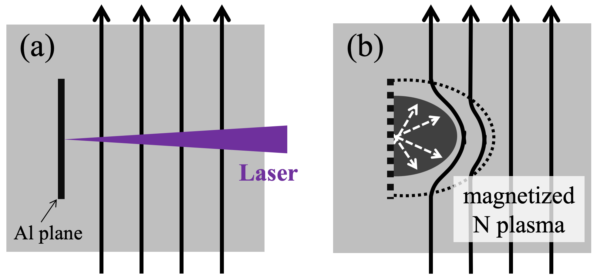
We used Gekko-XII HIPER Laser system (wavelength 1053 nm, pulse duration 1.3 ns, energy 690 J per beam, focal spot size 2.8 mm). An aluminum (Al) plane target with thickness 2 mm was irradiated by four beams simultaneously, resulting laser intensity of W cm-2 on the target. A schematic side view of the target and laser configuration is shown in Fig. 1. Before the laser shot, the chamber was filled with ambient nitrogen (N) gas with pressure Torr. Just before the shot, the external magnetic field ( T) was applied. The ambient gas was ionized by ionizing photons from Al plasma, becoming magnetized plasma with N ion density cm-3. Subsequently, Al plasma (dark gray region in Fig. 1(b)) pushed the magnetized N plasma to generate a magnetized collisionless shock (dotted curve in Fig. 1(b)).
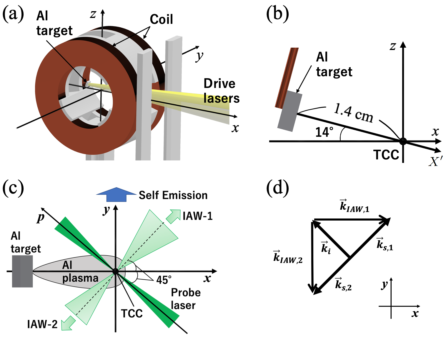
As shown in Fig. 2, the -axis is the vertical, and the central axis of coils is along the -axis. The target chamber center (TCC) is located at . Separation between the target surface and TCC was 1.4 cm, and target normal was . The external magnetic field was applied using an electromagnetic coil consisting of four 50-turn coils connected in parallel. The inner and outer diameters of the coils were 60 and 110 mm, respectively, and two of them were placed at mm, to generate almost uniform magnetic field perpendicular to the plasma expansion direction as shown in Figs. 2(a) and 2(c). This electromagnetic coil was driven by a small pulse-powered circuit Edamoto et al. (2018) consisting of four capacitors ( mF), each charged with a voltage of 1.4 kV, resulting in a quasi-static current of 5.3 kA in each coil and a uniform magnetic field of 3.6 T inside the coils. The time duration of the field of approximately 100 s is sufficiently larger than the typical timescale of the plasma propagation, and this field is quasistatic during the plasma expansion.
Using streaked optical pyrometry (SOP), the time evolution of the plasma self-emission (at a wavelength of 450 nm) along the target normal (-axis) was observed from the direction. The plasmas were also diagnosed with collective laser Thomson scattering (TS) method Sheffield et al. (2010). A probe laser (Nd:YAG, wavelength 532 nm, energy 370 mJ in ns) with wave number went through the plasma in the horizontal plane, , at an angle from the and -axis (-axis: see Fig. 2(c)). The scattered light with wave number was detected from two directions both of which are from the incident direction. As a result, one of the measurement wave number, , is toward the -axis, and the other toward the direction (Fig. 2(d)). Triple grating spectrometers were used to achieve a good spectral resolution of and pm for IAW-1 and IAW-2, respectively Tomita et al. (2017); Morita et al. (2019). We recorded the scattered light of ion feature with an intensified charge-couple device (ICCD) with 3 ns exposure time. In this paper, we discuss the role of self-generated field (via Biermann battery effect) in Al plasma Umeda et al. (2019). Unfortunately, there was no direct measurement of magnetic fields in this experiment to conclusively indicate that the Biermann field is playing an important role.
Before this experiment with N gas, we had performed similar experiments but with different ambient gas, hydrogen and helium. This was because it had been expected that the ion gyro radius and period could be small if the gas were fully ionized, which would help us make the field of view of our plasma measurement smaller. The use of a simple gas would make physical interpretation clear. Using Gekko-XII HIPER Laser system, we had various shots with different total laser energy and intensity, changing the number of beams and/or focal spot size. However, our TS measurements could not identify hydrogen or helium plasma at rest in the upstream region sufficiently before the Al piston plasma arrived. Hence, we concluded that photoionization of hydrogen or helium gas was difficult for our experimental setup, at least for lasers like Gekko-XII HIPER lasers. The reason is that the number of ionizing photons for hydrogen or helium gas is too small. For example, photoionization cross section for hydrogen atom takes maximum at the photon absorption edge ( eV), and above this photon energy, the cross section approximately scales as , where is the photon energy. Typical photon energy from target plasma just after the shot is keV in our laser intensity range, hence the photoionization cross section becomes very small, cm2. Then, the mean-free path of photons with energy keV is cm, where is the hydrogen gas density. Our system size is 1–10 cm, so that only a small fraction of keV photons ionize the hydrogen atoms, resulting in a very small ionization fraction. On the other hand, since the absorption edge is much higher for nitrogen ( eV, depending on charge states of N ions), the photoionization cross section for the nitrogen atom is much larger (cm2 for keV), which makes the upstream plasma generation much easier.
III Analysis of experimental data
III.1 Analysis of plasma self-emission
III.1.1 Case of
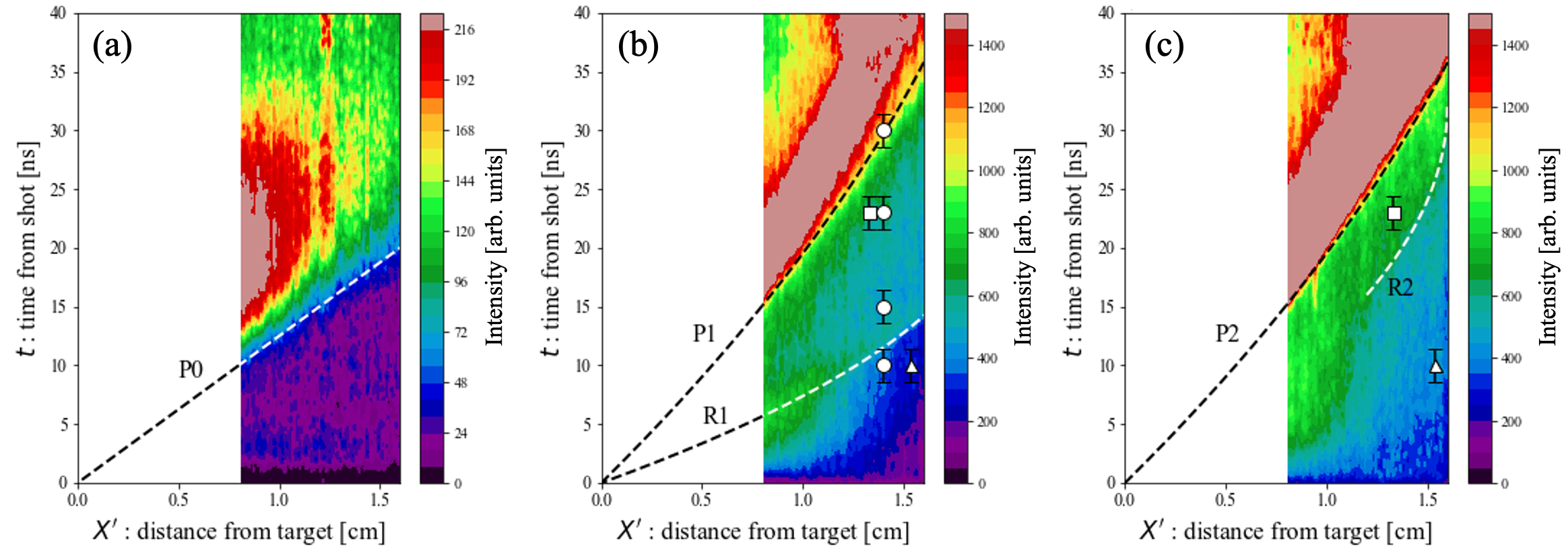
First, we show the SOP result (Fig. 3(a)) of a shot without ambient gas and external magnetic field () to clarify the properties of piston (Al) plasma. The Al plasma weakly emits light and freely expands with density decreasing with time.
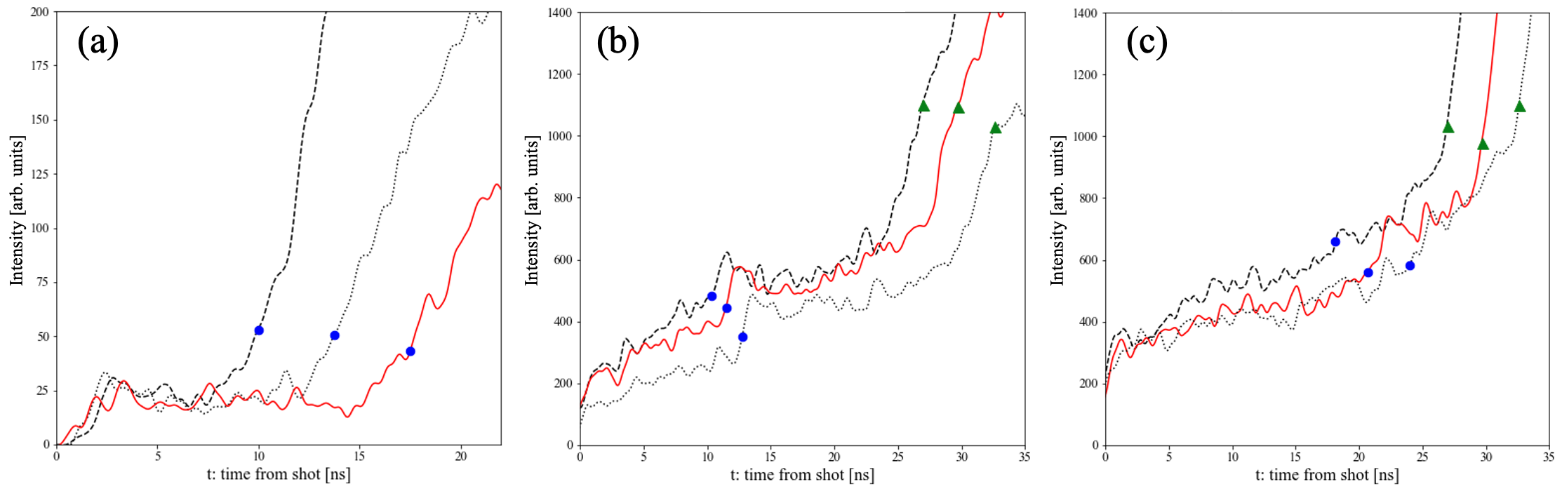
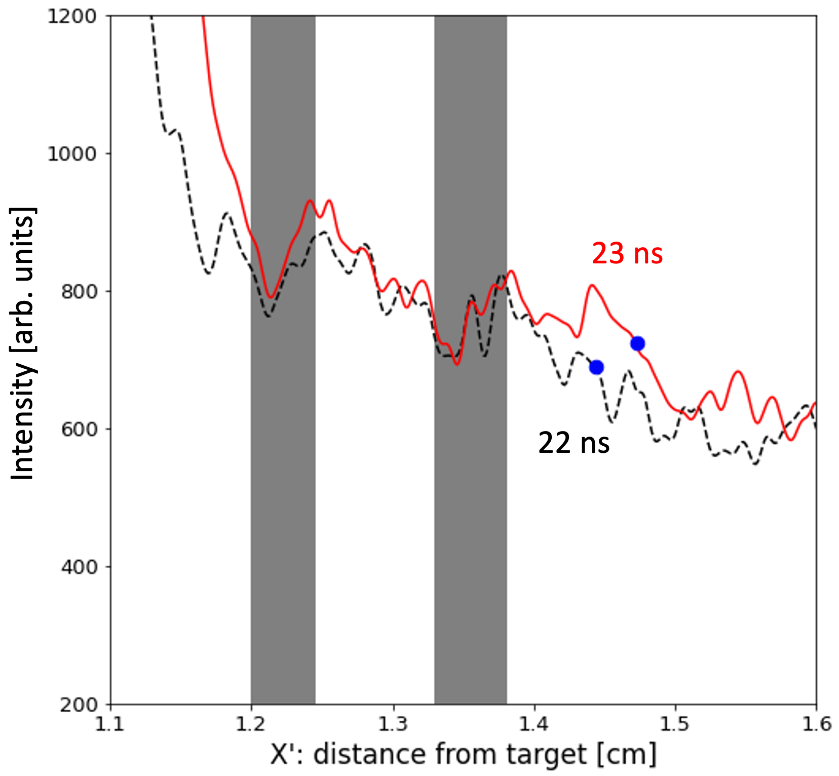
We show in Fig. 4(a) the time evolution of SOP counts at fixed positions , 1.1, and 1.4 cm (TCC). After the shot, the background intensity is on average in our unit, and it is variable because of statistical fluctuation. This may come from stray light of HIPER lasers, probe laser for TS measurement, and streak detector noise. After a while, the intensity starts to increase when Al plasma arrives; for example, at cm (black-dashed line in Fig. 4(a)), the intensity becomes twice the background level () at ns. Assuming that the Al plasma is freely expanding, we estimate the head speed of the Al plasma cm ns km s-1 (see blue circles in Fig. 4(a)). The line “P0” in Fig. 3(a) represents with a constant velocity km s-1.
III.1.2 Case of Torr and
Second, we had a shot with ambient N pressure Torr but without external magnetic field (). The result of SOP is shown in Fig. 3(b). The interaction between Al and N plasmas made much brighter emission than in the case of . The edge of the brightest part (denoted by “P1” in Fig. 3(b)) propagates with a speed km s-1 at ns. The more rapid structure “R1” goes ahead of P1 with a velocity of km s-1 at ns. If P1 and R1 arise at the target () at , they cannot be explained by constant-velocity motions. Instead, assuming a quadratic function of time, we determined their trajectories as described below.
We obtained the functional form, , of P1 as in the following. First, we made spatial profiles of the self-emission intensity (for fixed time) every 1 ns from 15 to 35 ns. Second, we found that the regions with SOP count of (yellow region in Fig. 3(b)) have large intensity gradient, whose scale length is mm. Hence for each time, we found the value of coordinate at which SOP count equals 1000, and we regard the points as the position of P1 at each epoch. Third, we adopt a quadratic function of time,
| (1) |
where constants and are initial velocity and a break time, respectively. Using this functional form, the points are fitted with least-squares method to get km s-1 and ns. Here, error means statistical in the fitting. Soon we will apply the same method to similar edge structure “P2” in the case of Torr and T (Fig. 3(c)), and derive similar values of and . They coincide with each other within errors, so that we adopt common values km s-1 and ns in dashed lines for P1 and P2 in Figs. 3(b) and 3(c), respectively.
For the structure R1, we could not apply the same method as for P1, because the SOP count variation (that is, the density gradient) around R1 is much less than P1. Scale length of the gradient of R1 is mm, so that it is difficult to define the positions of R1. Hence fitting by eye, we determined parameter values of and . Fortunately, one can see from Fig. 3(b) a clear boundary around –1.5 cm for –12 ns. In Fig. 3(b), we draw the dashed line as R1 along with this boundary, assuming the functional form given by Eq. (1) with km s-1 and ns. It can be confirmed from Fig. 4(b), showing the time evolution of the intensity at fixed positions , 1.4, and 1.5 cm, that R1 is in the period of abrupt intensity increase.
III.1.3 Case of Torr and T
Third, we performed a shot with Torr and T. Clear difference of SOP results between with and without external field cases can be seen (Figs. 3(b) and 3(c)). A small jump (denoted by “R2” ) is identified at cm at ns at which we had a TS measurement (see also Fig. 5). The location of the edge of the brightest region, P2, is almost the same as P1 at any time. Separation between R2 and P2 is smaller than that between R1 and P1 in the case of , suggesting that ion dynamics is changed by the external field.
As already described previously, we determined the trajectory of the structure P2 as in the same manner for P1. It is found that P2 is explained by the functional form given by Eq. (1) with fitted values km s-1 and ns, which coincide with the values for P1 within errors. This result is naturally understood if we assume that P1 and P2 are interface between Al and N plasmas (see § IV). Then, the ram pressure of Al plasma is so large that the presence or absence of the magnetic pressure in the N plasma is negligible at least in early epoch. The intensity change is sharper for T case than case; however, the physical interpretation of the observed width of the intensity gradients is difficult because there are many possible explanations (see § A.2 for details).
For the structure R2, when we determine the values of and , the situation is similar to the case of R1 in the case of T case than . SOP count variation is small and scale lengths of the intensity gradient of R2 is mm, making it difficult to define the position of R2. Nevertheless, one can identify the boundary of green region in Fig. 3(c) for –25 ns. Assuming again the functional form given by Eq. (1) with km s-1 and ns, we draw the dashed line R2 in Fig. 3(c). As in the case of R1, one can see from Fig. 4(c) that around R2, the rate of intensity increase becomes higher than before. Figure 5 shows the spatial profiles of the self-emission at and 23 ns, that is, one-dimensional slices of Fig. 3(c). Despite fluctuation via instrumental pixel damage and statistical noise, we identify an intensity decrease from to 1.5 cm at ns at which we performed TS measurement. Comparing with the profile at ns (black-dashed line), one can see that R2 propagates outward.
Again as seen in Fig. 3(c), self-emission intensity is inhomogeneous upstream of R2. This fact is similar to the case of Torr and . (see § A.1 for detailed discussion).
III.2 Analysis of Ion term of Collective Thomson scattering (TS) spectra
We fit TS spectra assuming the resonance with ion-acoustic waves (IAWs) in plasmas, which have a single ion-component in Maxwelian distribution. The IAW spectrum is fitted with a convoluted spectral density function
| (2) | |||||
| (3) |
where is the resolution of the spectrometer evaluated from the Rayleigh scattering and expressed as a Gaussian, and are electron susceptibility and longitudinal dielectric function, respectively, , , is the ion distribution function, and the charge state is self-consistently derived from a collisional radiative model with the FLYCHK code Chung et al. (2005). The TS scattered light intensity is proportional to the electron density , and it is determined by an absolute calibration of the collective TS system using the following formula:
| (4) |
where , , and are the light intensity, cross section, and incident laser energy, respectively, the subscripts “T” and “R” represent the Thomson and Rayleigh scattering, respectively, is the nitrogen density for Rayleigh scattering measurement, and is the total intensity of the ion component expressed as . Errors for plasma parameters by TS measurements are evaluated from best-fitted values and covariance that we get from the least-squares fitting of the observed IAW spectra.
Results are summarized in Table 1, where we assume N plasma except for the case of rapidly moving ( km s-1) component that is seen by IAW-1 at around nm at ns, (TCC), and (Fig. 6(b)) and the case of ns, (TCC), and (Fig. 6(d)). For these cases, we show in the table both results on the assumption of N and Al plasmas.
As stated above, we analyzed IAW spectra on the assumption of a single component plasma with Maxwell distribution. In our case, the distribution function deviates from Maxwellian around the shock transition layer. However, at present, analysis method in such a case has not been established, because we have no matured theory of TS spectrum in that case. This issue may be a future problem to be resolved in the community of shock experiments. Hence, we cannot help but say that derived parameters, listed in Table 1, are just approximate values guiding our theoretical interpretation.
III.2.1 Case of Torr and
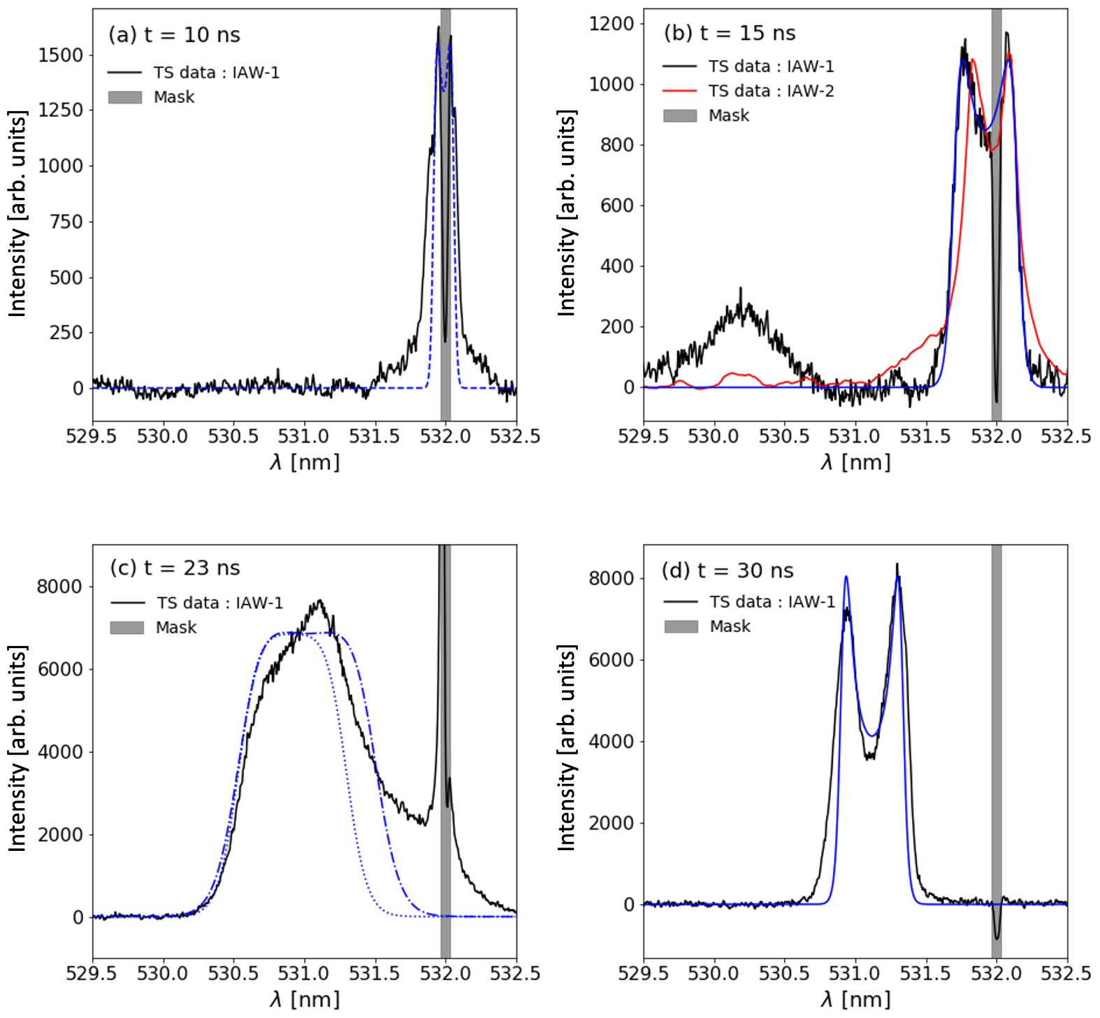
In Figs. 6(a) and 6(b), two peaks corresponding to the resonance with IAWs are seen at around 532 nm. These are from upstream N plasma almost at rest. Just before the arrival of R1 at TCC ( ns), we identify almost at rest, cold (, eV) N plasma (Fig. 6(a): see § B.1 for further discussion). A few ns after the passage of R1 ( ns), the static N plasma was heated ( eV and eV). We also identify the moving plasma at nm from IAW-1 but not from IAW-2, showing the ion dynamics is collisionless (see also § E.2). Assuming this component is moving along the -axis, we derive the bulk velocity km s-1 (see § B.2), which is roughly consistent with the velocity of R1 at ns.
The TS spectrum taken at ns () does not show a clear double peak (Fig. 6(c)). If we fit the spectrum in the same way as the other epochs, so that assuming that the observed spectrum is made by IAW in plasma with Maxwell distribution, then we derive unnatural parameters: namely, electrons would move toward target with bulk velocity of km s-1. This indicates that the plasma in this epoch and space is nonstationary and/or in highly nonlinear regime. In any case, the spectrum seems to show high ( keV: see blue dotted and dot-dashed lines in Fig. 6(c)). The TS spectrum at ns reveals plasma with a clear double peak with km s-1 (Fig. 6(d): see § B.3).
III.2.2 Case of Torr and T
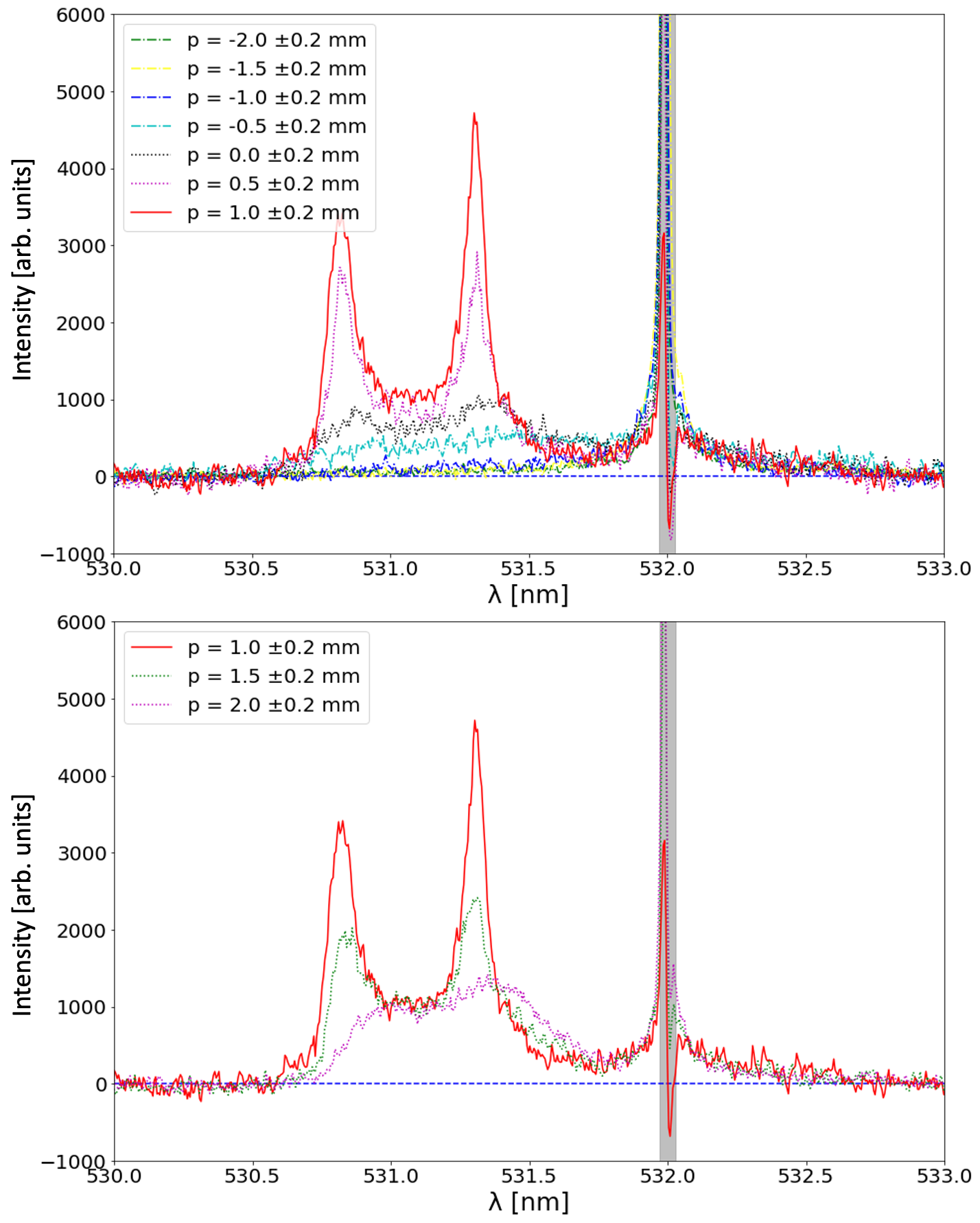
Next, we analyzed the data of a shot with Torr and T. Figure 7(a) shows the TS spectrum at ns, where the vertical -axis represents the position along the probe laser (see Fig. 2(c)), so that . A clear double peak of the ion-acoustic resonance is identified when . Assuming N plasma, we fit the spectrum at mm (Fig. 7(b)) and obtain km s-1 and the ion density cm-3 which is about 3.6 times as large as the initial upstream one, indicating the ion compression. Note that the double-peak feature in the TS spectrum still can be seen for mm, where sensitivity becomes weaker; however, the feature vanishes for mm (Figs. 7(a) and 9). Such an edge feature corresponds to R2 in Fig. 3(c), and it is first observed by spatially resolved TS measurement. In addition, as shown in Table 1, the density has a maximum at mm (see § B.4 for further discussion).
| T | |||||||||||
| 111Time from laser irradiation. | 222 corresponds to TCC (see Fig. 2(c)). | ||||||||||
| [ns] | [mm] | [eV] | [eV] | [cm-3] | [km s-1] | [eV] | [eV] | [cm-3] | [km s-1] | ||
| 333Assuming . | 2.8 | ||||||||||
| 0444Cold component. | d | d | d,f | 3.2d,f | d | ||||||
| 0555Warm component. | e | e | e,666Fixing N ion density, cm-3. | 5.0e,f | e | ||||||
| 0 | 5.5 | ||||||||||
| 0 | — 777Unconstrained. | 4.0 | |||||||||
| 0888Assuming Al plasma instead of N plasma. | h | — g,h | h | 4.9h | h | ||||||
| 0 | N/A (see text) | 6.7 | |||||||||
| 0.5 | N/A (see text) | 6.5 | |||||||||
| 1 | N/A (see text) | 6.4 | |||||||||
| 1.5 | N/A (see text) | 6.1 | |||||||||
| 0 | 5.1 | ||||||||||
| 0h | h | h | h | 10.3h | h | ||||||
IV Discussion
We performed 1D PIC simulations with similar conditions to our experiment. For details of the simulation set up, see Umeda et al. Umeda et al. (2019). We adopt the same parameters as those of Run 1 (and Run 2) of Umeda et al. Umeda et al. (2019), but we consider two cases with different external magnetic field strength in the N plasma, and T. In the Al plasma, the magnetic field with the strength of 10 T is externally imposed. This is a simple artifact of a self-generated Biermann field, although our 1D simulation cannot capture the developement of the field. Note that we use real electron-to-ion mass ratios and 25704 for Al and N plasmas, respectively. Our PIC simulation scheme does not incorporate the effects of Coulomb collisions.
Below we interpret our experimental results comparing with 1D PIC simulations. Such an argument is similar to previous experimental studies on supercritical magnetized shocks. Note, however, that as already stated in § I, laser experiments are possibly capable of seeing larger-scale, longer-time evolution of plasma interaction, which is currently unachievable with 3D PIC simulations with real mass ratio. This causes a dilemma when comparing experimental and simulation results since we cannot accurately evaluate multi-dimensional effects (e.g., non-plane-parallel plasma expansion resulting in adiabatic cooling and dilution of the Biermann magnetic field, excitation of obliquely propagating waves in highly inhomogeneous plasmas, and so on). Hence, we should not fully rely on the numerical simulation results, and it is not necessary that experimental results perfectly (quantitatively) match the simulation results. Nevertheless, as described below, our 1D PIC simulation results in both and 3.5 T cases are broadly consistent with experimental data, so that we believe that our simulations already catch essential features related on the magnetized shock formation.
According to our 1D PIC simulation for Umeda et al. (2019), the sharp rise of the electron density occurs at an interface between N and Al plasmas in the electron scale, so that we interpret P1 seen in SOP (Fig. 3(b)) as this electron-scale discontinuity. This is supported by the fact that high electron and ion temperatures are observed at and 23 ns, upstream of this interface. Our radiation hydrodynamics simulation (see § C) shows that the Biermann magnetic field in Al plasma has initial strength T, and as the plasma expands the field becomes weaker ( T at ns around the head of the Al plasma). It is at least partially responsible for the N ion reflection Umeda et al. (2019). Collisional coupling is also non-negligible (see § E.1 for details). Later the interface P1 decelerates due to the interaction between Al and N plasmas, so that its velocity decreases to km s-1 after propagating cm from target (at ns).
Our 1D PIC simulation for also showed that some Al ions penetrate beyond the interface, being accelerated by the ponderomotive force Umeda et al. (2019). These fast Al ions might correspond to R1 seen in Fig. 3(b) (see § D.1 for more discussion). The fact that the initial velocity of P1 ( km s-1) is smaller than implies that at least some Al ions penetrate upstream beyond P1. Another possible explanation of R1 is N ions reflected around the head of Al plasma. This might be indicated by our experimental result that the initial velocity of R1 ( km s-1) is just as twice as the initial Al velocity ( km s-1). During the propagation, such fast ions decelerate due to the interaction with upstream N plasma at rest, leading to the heating of incident N plasma between P1 and R1.
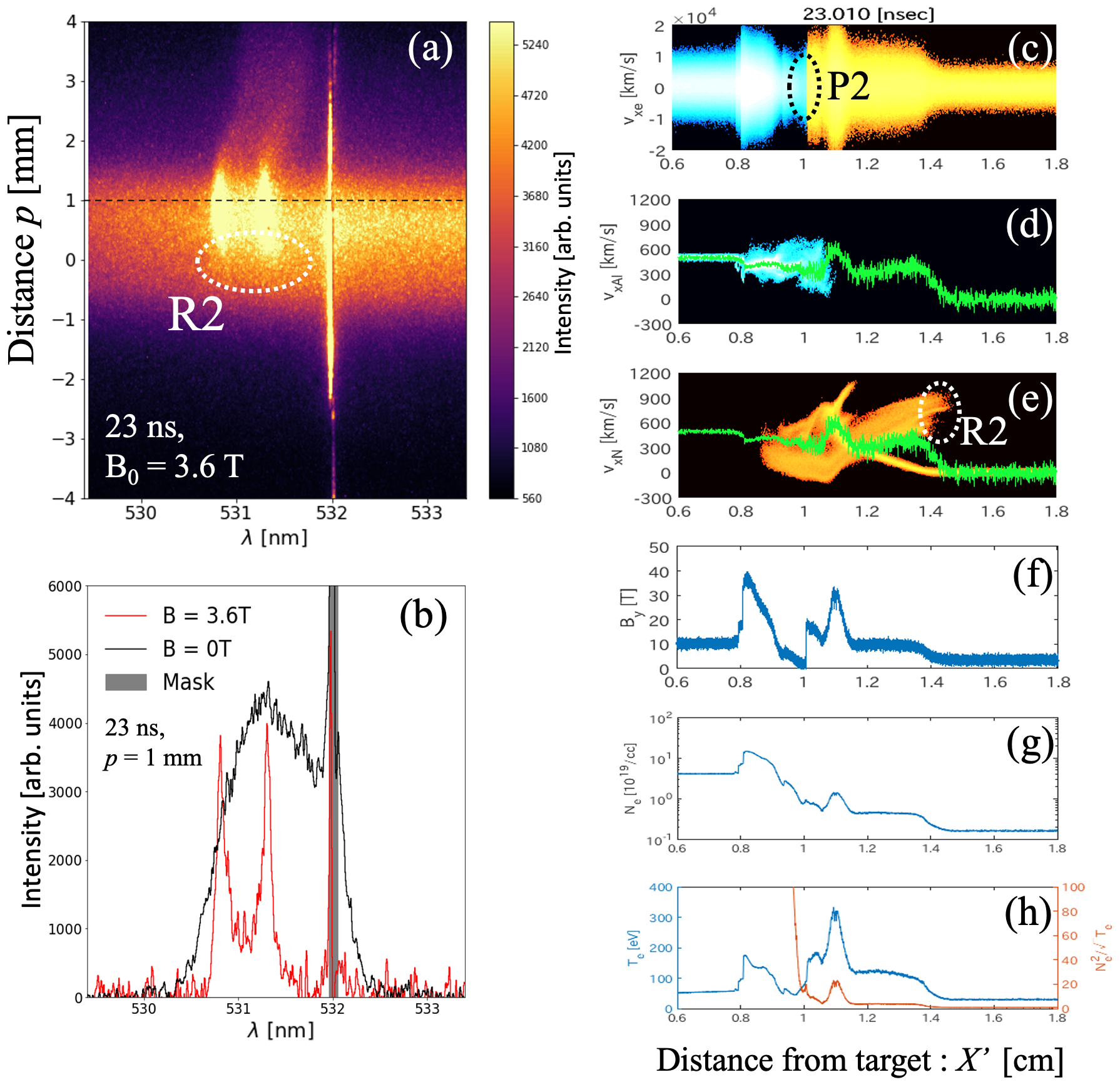
Our analysis results of SOP and TS measurements for T case are again broadly consistent with results of 1D PIC simulation with T (Figs. 7(c)-(h) and Fig. 12). Observed steep emission gradient P2 in Fig. 3(c) is associated with an interface between Al and N plasmas (see Fig. 7(c) and red line in Fig. 7(h)). Incident N ions do not penetrate deeply into the Al plasma because of compressed Biermann magnetic field (Fig. 7(f)) and/or collisional coupling. On the other hand, Al ions are trapped by compressed external magnetic field, and do not enter the N plasma (Fig. 7(d)). Incident N ions are initially reflected at the interface between Al and N plasmas (which is observed as P2 in Fig. 3(c)) and later reflected by the compressed external field in the N plasma (Fig. 12). They are gyrating back due to the external magnetic field (Fig. 7(e)), forming a shock foot. Hence, it is natural to interpret that R2 in Fig. 3(c) corresponds to the edge of the reflected N ions (Fig. 7(e)), which has also been confirmed by TS measurement (Fig. 7(a)). The density takes maximum at mm (Table 1), which is about to be a shock overshoot. Observed keV at mm of the reflected component is larger than incident N ions, but is smaller than that for (Fig. 7(b)). This is also consistent with PIC results. Therefore, we claim that the spatially resolved edge of the foot of a developing magnetized collisionless shock is measured (see § B.4, § D.2, and § E.3 for further discussion).
We estimate upstream physical quantities. We had only one shot with T, and TS spectrum at ns. Hence, we simply assume the upstream plasma parameters except for are the same as those for the unmagnetized case. We analyze the data of IAW-1 for the case of Torr and at ns and mm, at which the discontinuity R1 had not arrived yet (white triangle in Fig. 3(b)). We fit the TS spectrum to get the N ion density cm-3 (see § B.1), suggesting the upstream medium is fully ionized. Using the best-fitted values, we get upstream quantities such as the sound speed km s-1, Alfvén velocity km s-1, and ion (electron) plasma beta () for T. Simply assuming magnetohydrodynamics, we expect that the velocity of a forming shock may be higher than that of interface between Al and N plasmas (P2: see Figs. 3(c) and 7(c)), whose typical value is km s-1. Then, we expect the magnetosonic Mach number and Alfvén Mach number , so that the shock will be supercritical with ion-ion mean-free path cm.
V Summary
We have conducted experiments of generating collisionless shocks propagating into magnetized plasma at rest with uniform mass density. It is quite difficult to identify a shock formation only from SOP due to the bright emission enhancement at P2. However, our PIC simulations show that R2 is composed only of N plasma, and if we analyze the TS data assuming the N plasma, all the experimental data self-consistently show that R2 is an edge of the foot of a forming supercritical shock in the magnetized N plasma. We are also sure that a shock ramp and overshoot are arising between P2 and R2 as seen in the PIC result.
Appendix A Notes on SOP Analysis
A.1 On the inhomogeneity upstream of R1 and R2
As shown in Figs. 3(b) and 3(c), self-emission intensity is not uniform both upstream of R1 in case and of R2 in T case. This indicates the ionization of upstream N plasma is not uniform. Ahead of R1 and R2, neither Al nor reflected N plasma co-exist, so that the cause of the non-uniformity is likely time-dependent photoionization. Around the interface between Al and N plasmas (P1 and P2), the electron temperature is high and it can be more than 100 eV as shown by our 1D PIC simulations (Figs. 11 and 12). Such high-density, hot plasma emits ionizing photons, and they change the ionization state of the upstream N plasma. When photoionized, N ions eject hot electrons, resulting in the plasma heating. This causes further change of the upstream ionization state. Both collisionless and collisional processes depend on the ion charge state. However, the upstream number density of N ions (i.e., the upstream mass density, which determine the whole shock dynamics from ion scale to hydrodynamical scale) is still uniform.
A.2 Observed width of the density gradients
In ideal plane-parallel case, width of the transition layers P1 and P2, which are the interfaces between the Al and N plasmas in electron scale, is given by the gyro radius of thermal electrons around the layers if Al and N interaction is collisionless. It is estimated as . The mean-free path of electrons via electron-electron Coulomb collision is on the same order or less. These lengths are much smaller than the observed apparent width mm or slightly less. This discrepancy is explained by the three-dimensional (3D) effect: geometry of the plasma self-emission in 3D space is not plane parallel, and even the interface fluctuates during the propagation. In such an actual case, the emission is projected onto the detector plane whose normal vector is in the direction. As an extreme toy case, let us consider spherically symmetric uniformly emitting sphere with radius whose emissivity is given by step function, for and for ( is the radial coordinate in the spherical coordinate system). When such emission is projected onto the detector plane, the apparent spatial profile does not remain step-function-like, but has gradual transition whose width is on the order of the curvature radius . More generally, in cylindrically symmetric case, the projected emission profile is related to the emissivity in the three-dimensional space by Abel transform. In the present case, the exact plane parallel assumption is clearly not a good approximation, although the local curvature radius of the interface is highly uncertain. However, the length on the order of 0.1 mm is not unnatural. These projection effect may become important for not only P1 and P2 but also the other emission gradients R1, R2 and P0.
There are several other possibilities to explain the observed width of P1 and P2, such as Rayleigh-Taylor instability and the inhomogeneous expansion of the Al plasma (that is, anisotropic velocity distribution of kinetic energy of Al plasma). As another case, when the Biermann field in Al plasma is weak ( T), the diffusion length of electrons in the direction perpendicular to the Biermann field is potentially comparable to the observed scale width . At present, precise description of the observed width is difficult since there are several physical possibilities.
Appendix B Notes on Analysis of TS spectra
B.1 TS spectra at ns for
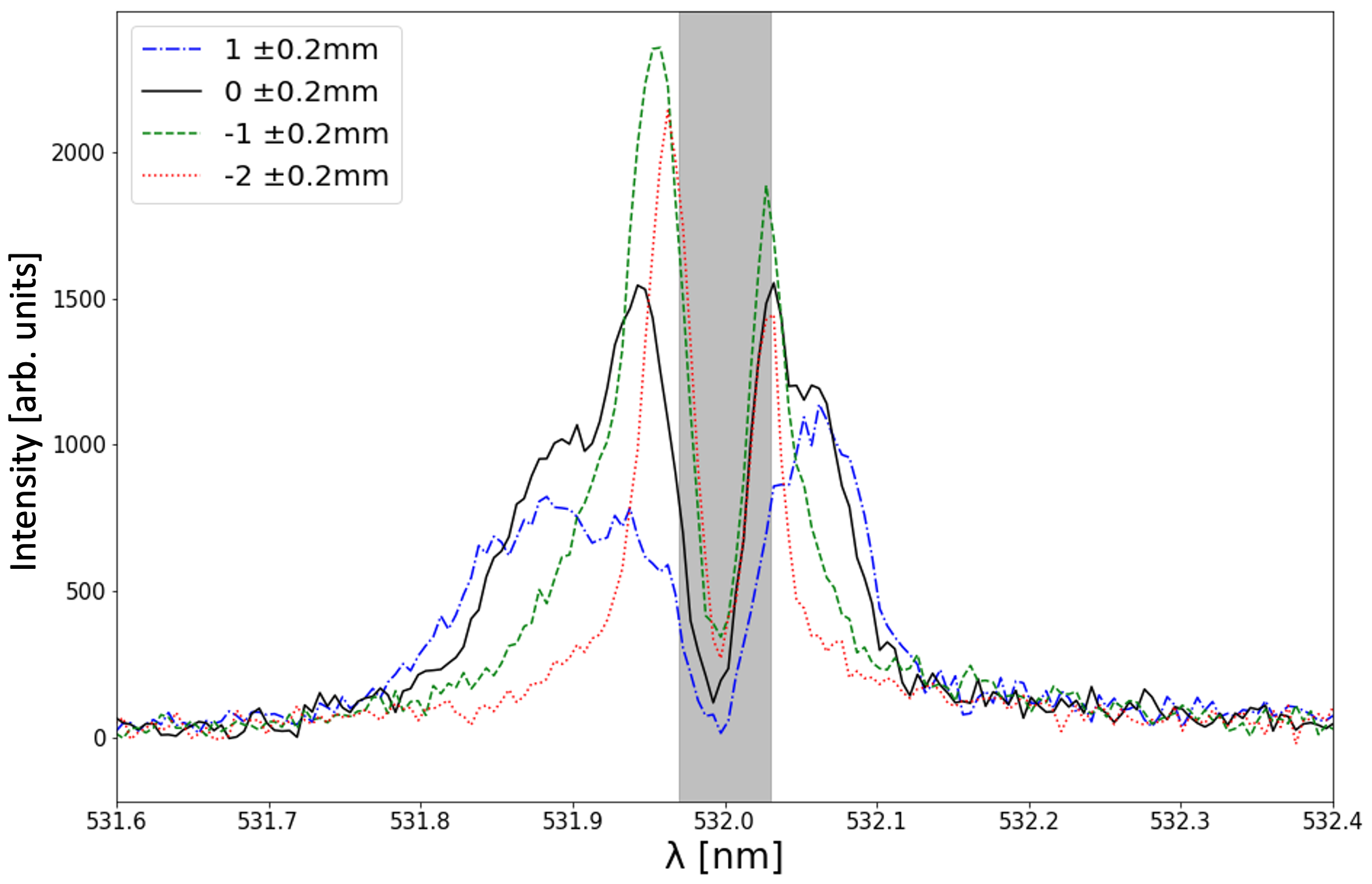
We show in Fig. 8 the IAW-1 (see Fig. 2(c)) spectra at ns around nm with different positions , , 0, and 1 mm. The black solid line in Fig. 8 (, TCC) is identical to the black solid line in Fig. 3(a).
We see TS spectra from N plasma at rest. During the instrumental gate width of 3 ns, the rapid plasma component R1 (shown in Fig. 3(b)) passed around TCC. Such rapidly moving plasma has a large Doppler shift, so that its scattered light does not exist around nm, and may be even outside of the whole range of wavelength coverage of our spectrometer system. (If we assume the plasma velocity corresponding to R1 as km s-1 with km s-1 and ns, then the Doppler shift nm is predicted.) The component R1 electrostatically interacts with the incident N plasma, resulting in rapid heating of the N plasma. This is also suggested by the rapid increase of self-emission at TCC (see Fig. 4(b)).
The position mm was in the region at which the rapid component R1 had not arrived yet, so we interpret that the TS spectrum at mm comes from the upstream N plasma that was unaffected by Al ejection. This is also justified by our 1D PIC simulation (see § D.1). Then we fitted the spectrum assuming , and best fitted parameters are shown in Table 1. At mm, we also see such a cold component, but slightly heated compared with the case of mm. At mm, which becomes the downstream region of R1 near the end of exposure of TS measurement, one can see warmer plasma with broader separation between double peaks of IAW resonance.
The TS spectrum at (TCC) looks complicated. It seems to consist of the two superimposed components (cold and warm N plasmas). First, we fit the spectrum in the wavelength range nm (excluding the gray-shaded region shown in Fig. 8 that is affected by a filter to cut the stray light) in order to explain only the cold component with narrower separation of the double peak. Assuming and , we derived eV, cm-3, and , which was represented by the blue dashed line in Fig. 6(a). Then one can clearly see that the fit outside of the fitting wavelength range is inadequate, which indicates the existence of another warm component. Hence, we next fit the TS spectrum with two components that are simply superimposed, where we assume the two components are recorded in the instrumental gate width of 3 ns. In fitting the data, we fix the N ion density cm-3. The best-fitted parameters are shown in Table 1. Note that both cold and warm components are almost at rest, so that both are highly likely N plasmas.
B.2 TS spectrum at ns for
B.3 TS spectrum at ns for
Figure 3(b) shows that at ns, the interface P1 passes through TCC ( cm, ). Hence, the observed TS spectrum may either come from Al or N plasma, so that we fit the spectrum for both cases. Indeed, it is hard from the best-fitted values shown in Table 1 to judge which plasma is responsible for the observed spectrum. In the case of N plasma, both the electron density cm-3 and the ion density cm-3 are several times as large as initial N plasma densities. This fact is naturally explained by 1D PIC simulation. However, we cannot exclude the cases of Al plasma.
B.4 TS spectrum at ns for T
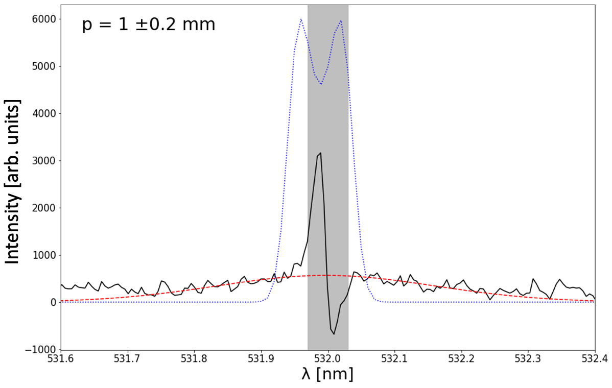
If R2 is the edge of reflected N ions, there should be another N ion population at rest as seen in 1D PIC simulation at around nm in the TS spectrum (e.g., Schaeffer et al. (2019)). Since the observed data contains bright self-emission as a background and there is intense stray light around the probe laser wavelength ( nm), it is difficult to perform the spectral analysis to find such a component. Using data in the wavelength ranges –530 nm and 533–534 nm, we determined the background by fitting with a cubic function. The background-subtracted spectra are shown in Fig. 9. One can find small excess around 532 nm. Assuming the TS ion feature from N plasma, we fitted the excess component. For mm, we obtained cm-3 and eV, though the electron temperature is unconstrained since the observed intensity is weak (red-dashed line in Fig. 10). Then, we calculate a parameter , where is the electron Debye length, and hence the ion-term scattered light becomes dim. We also estimate a parameter that determines the shape of the ion term Sheffield et al. (2010), and we have for small , so that it is less than unity as long as eV. In such cases, the TS ion term has a single peak as shown by the red-dashed line in Fig. 10.
In the case of the fitting result shown above (red-dashed line in Fig. 10), the derived value of is about one order of magnitude smaller than expected. If there were the same N plasma with cm-3 as seen for the case of , ns, and mm (see Table 1), which we refer to as upstream N plasma in this paper, then the TS spectra would have seen by the blue-dotted curve in Fig. 10. If we rely on 1D PIC simulation results, the electron temperature alone increases to more than 100 eV around mm. In this case, the ion acoustic peaks in the TS spectrum would be more separated from 532 nm, so that we would more clearly see the component although the ion-term scattered light would be dim because the scattering is in the noncollective regime (). Hence, we could not experimentally identify the coexistence of incident N plasma almost at rest with low ion temperature and electron density of cm-3. From the experimental view point, a probable explanation of the observed excess around 532 nm is the stray light of the probe laser.
As discussed above, in our present experiment we could not identify another N ion population almost at rest, coexisting with the R2 component, which is indicated in 1D PIC simulation. However, we should not directly believe the result of 1D PIC simulations in this case. In the 2D or 3D case, plasma interaction proceeds more rapidly, and incident N plasma becomes dilute in velocity space. As a result, the two components are mixed with each other and merge into a single population in the velocity space. Another possibility to disentangle this issue is that the plasma temperatures, and , of the expected component are smaller than eV. Then, TS spectrum from such a cold plasma has narrow peak, and in our present spectrometer system, it is masked by a filter to cut stray light. Such a case potentially occurs because the upstream state is inhomogeneous (see § A.1) — the less ionized are N ions, the less hot electrons, resulting in the lower temperatures and less electron density. There may also be the collisional effects. Finally, we emphasize again that in our analysis of TS ion term, we have assumed Maxwell distributions of ion and electrons and radiative-collisional equilibrium, which are clearly violated in the shock transition layer. The derived plasma parameters by our present analysis might be different from actual values.
Appendix C Estimate of the Biermann Battery Magnetic field
We performed 2D radiation hydrodynamics simulation Ohnishi (2012) to have electron pressure and density of Al plasma ejected by laser irradiation. Then, in order to estimate the strength of the Biermann magnetic field in the Al plasma, we solve, as a post process, the induction equation with Biermann term
| (5) |
to get the evolution of the field. It is found that until 4 ns from the shot, the magnetic field strength in the Al plasma is more than 100 T at the point where the electron density is equal to the critical density of cm-3. Note that even in this case, the plasma beta is not less than unity, so that the generated magnetic field does not alter the overall dynamics of Al plasma. After that, the plasma expands and the field strength becomes small (e.g., T at ns around the head of Al plasma); however, it is still strong enough to reflect N ions into Al plasma. Our simulation result on the field generation is quantitatively consistent with previous numerical studies Schoeffler et al. (2014, 2016); Fox et al. (2018).
Appendix D Details of 1D PIC simulation results
D.1 Result for T
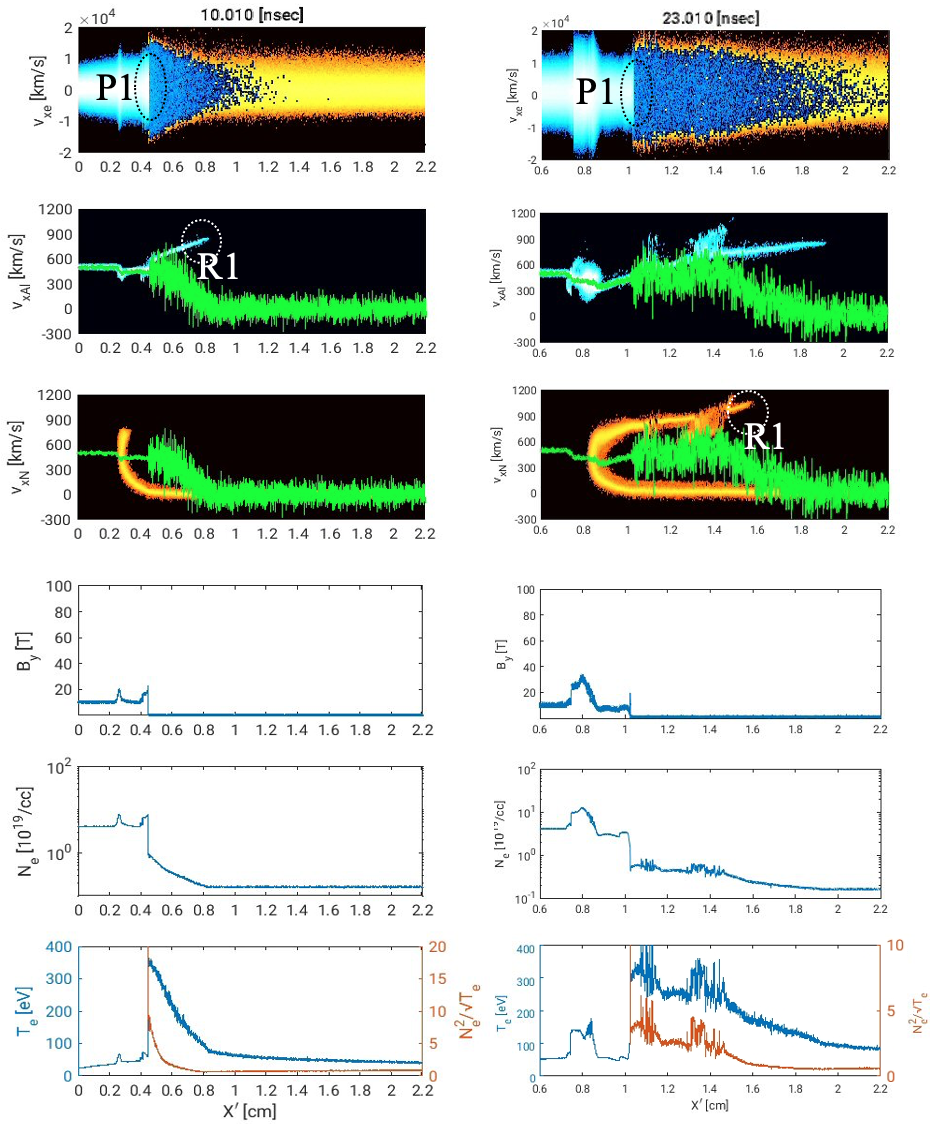
This case is identical to Run 2 of Umeda et al. Umeda et al. (2019). Results for ns was presented in Fig. 4 of Umeda et al. Umeda et al. (2019), which shows the electron-scale tangential discontinuity at cm. The electron density rapidly increases there. We interpret this discontinuity as corresponding to the structure “P1” found in SOP.
In Fig. 11 we show the results for ns and ns, the latter of which can be directly compared with Figs. 7(c)–7(h). A part of Al ions penetrates into incident N plasma after accelerated by ponderomotive force at the interface (P1) between Al and N plasma. At ns, it reaches the position cm. As shown in the electron phase space plots (top panels of Fig. 11), a small fraction (%) of electrons originally associated with Al ions, shown by blue dots in the right-side region of P1, that is, electrons injected at the left boundary , go across the interface P1. (In the phase space plots, deeper blue means less number of particles, while light blue or nearly white regions indicate high particle density.) Nitrogen ions are being reflected by the Biermann magnetic field in Al plasma; however, its edge is still in the Al plasma (that is, in the left region of the interface P1 at cm). Interaction between the penetrating Al plasma and incident N plasma is responsible for plasma heating and enhancement of the plasma self-emission upstream of P1 (–0.8 cm). Hence, we interpret the tip of penetrating Al plasma corresponds to the structure “R1” found in SOP in the early epoch. In our 1D PIC simulation, the region around TCC ( cm) is unaffected by the penetrating Al plasma. Namely, the position mm (definition of -axis is shown in Fig. 2(c)) corresponds to cm, hence it is expected that the observed IAW-1 TS data at ns and mm is appropriate to estimate the parameters of initial upstream N plasma.
At ns, penetrating Al plasma reaches the position cm. Nitrogen ions are reflected by Biermann magnetic field in Al plasma, and the edge of the reflected component arrives at cm. Before reflected N ions come back, incident N plasma is heated just after the passage of Al ions by electrostatic interaction (–1.9 cm), and electron temperature becomes larger. When we calculate the spatial profile of the intensity of the plasma self-emission (assuming the bremsstrahlung emission, ), we find that it starts to increase at the edge of the reflected N ions at cm. Hence, we interpret this edge corresponds to the structure “R1” found in SOP in later epoch.
Our 1D PIC simulation used typical parameters of Al and N plasmas around TCC ( cm) at late epoch (e.g., –30 ns) Umeda et al. (2019). The high-speed flow at 1600 km s-1, labeled as “R1”, is not seen in the 1D PIC simulation. On the other hand, parameters of Al plasma and N plasma around the target in the experiment are quite different from those of the 1D PIC simulation. For example, Biermann magnetic field in Al plasma is estimated as T at the initial state of the experiment by radiation hydrodynamics simulation. Such a strong magnetic field may generate a high-speed flow at 1600 km s-1 in 2D/3D system. Then, the position of the emission edge “R1” found in SOP may be much farther from the target. Nevertheless, it can be said that our PIC simulation qualitatively well explains our experimental results.
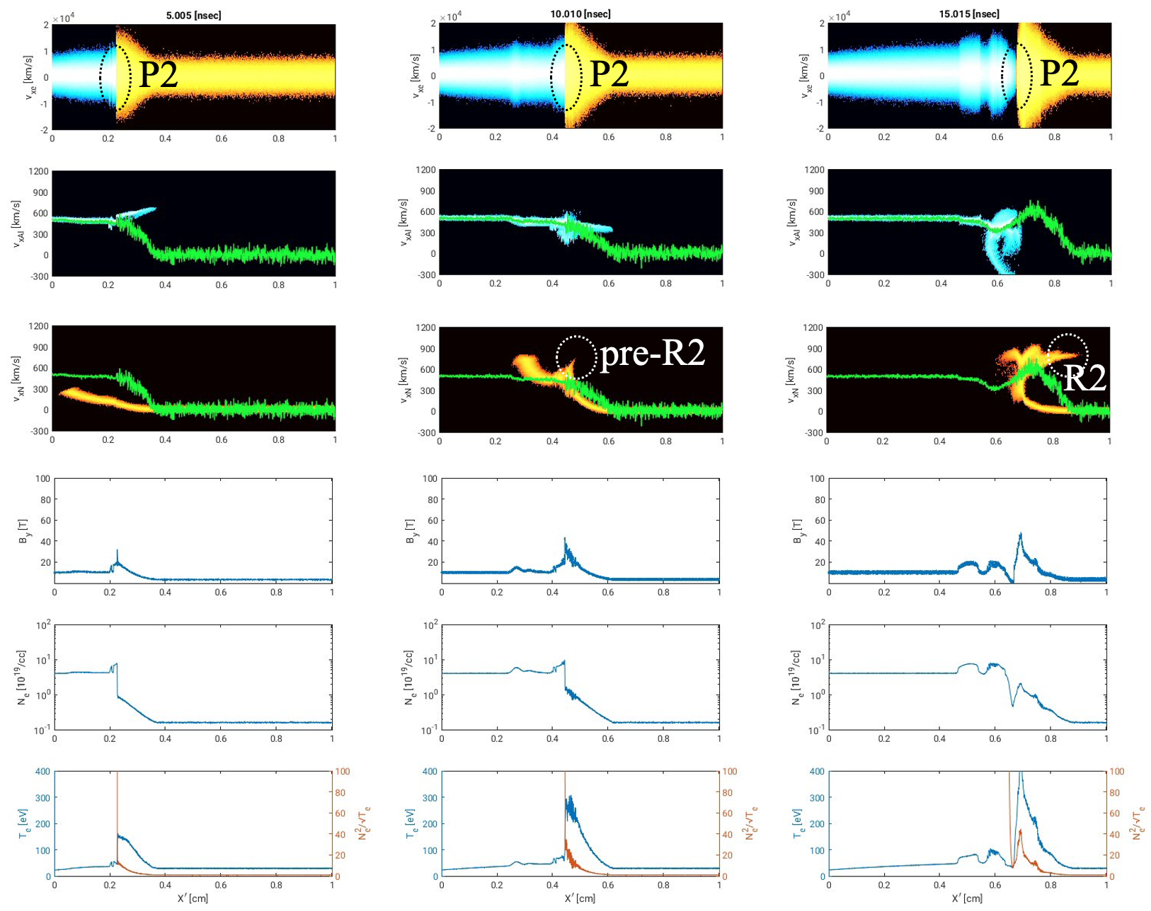
D.2 Result for T
The results at , 10, and 15 ns are shown in Fig. 12. After ns, incoming N ions are reflected at the region of strong magnetic field that is the compressed external field (center and right panels of Fig. 12). The reflection point is then the upstream side of the interface between Al and N plasmas (structure “P2” shown in Fig. 12, and in Figs. 3(c) and 7(c)). Hence, after ns, incoming N ions are reflected in the N plasma. These reflected N ions form the structure “R2” (see Figs. 3(c), 7(a), and 7(c)). The N ions reflected at ns are responsible for “R2” at ns. In earlier epoch ( ns: left panels of Fig. 12), incoming N ions penetrates into Al plasma and they are reflected by the Biermann field in the Al plasma (left panels of Fig. 12). However, such ions have already come back to N plasma before ns, and have turned again by the external field, going back toward the downstream region (it has been passed 0.7 times the ion gyro period). Hence, they are not at the edge R2 when ns, but at around –1.0 cm.
Appendix E Effects of Coulomb collisions
In this paper, we have mainly considered collisionless processes. However, collisional effects are not negligible in some cases. Our current 1D PIC simulations do not capture the role of Coulomb collisions. The mean-free path of electron-electron Coulomb collision is smaller than any other scales in most cases with typical parameters, so that electrons are hydrodynamically coupled. Below, we discuss effects of ion-ion collisions for structures P1, P2, R1, and R2. In the following, we adopt an approximate formula of the mean-free path of ions with mass , charge , and initial velocity , running into the plasma with ion mass , charge , electron density , ion density , electron temperature , and ion temperature , which is given by , where and the mean relative velocity . The Coulomb logarithm is calculated with , where , and and are electron and ion Debye lengths, respectively Spitzer (1965); Pauls et al. (1995).
E.1 Structure P1 and P2
Our claim is that N ions penetrating into Al plasma is reflected by Biermann magnetic field in the Al plasma. Although the Al plasma parameters are uncertain at times and positions of our interest, we set eV, , the ion density cm-3, and the magnetic field strength T as typical values. A trajectory of P1 and P2, , gives the velocity, , of 510 km s-1 at ns, and of 406 km s-1 at ns, so we set the relative velocity km s-1 as a fiducial value. The mean-free path of N ions with in the Al plasma is then , and gyro radius of the N ions is given by , where and , so that their ratio is . When we only change temperatures to eV, then we get . If with the other parameters being fiducial, the ratio becomes . In these cases, although Coulomb collision is marginally subdominant, it is non-negligible. However, at least, it can be said that the Biermann field plays a crucial role in N ion reflection in the Al plasma. Note that while the electron-electron Coulomb collision mean-free path is much smaller than and , electrons around P1 and P2 cannot generate an electric field that is able to reflect incoming N ions.
E.2 Structure R1
An explanation of structure R1 is fast Al ions penetrating into initial upstream N plasma as shown in our 1D PIC simulation. The mean-free path of the Al ions with in the N plasma ( eV, , and the N ion density cm-3 corresponding to Torr) is estimated as , where . If R1 is the head of N ions reflected by interface P1, their mean-free path is also large ( cm for reflected ion charge number –6). Hence, the collisional effect is negligible for the propagation of R1.
E.3 Structure R2
Our claim is that R2 at ns is the edge of N ions that are reflected by compressed external magnetic field in the N plasma just upstream of P2 at ns. Although the parameters of the N plasma at the reflection region are again uncertain, we set eV, eV, the electron density cm-3, and the strength of the compressed external field T, considering the result of our 1D PIC simulation at ns. The value of is also uncertain but for the worst case, we assume that both incoming N ions and the N plasma have . Then we obtain the ion-ion mean-free path of incoming N ions and their gyro radius , where and . Hence, the ratio of these scale length is . According to our PIC simulation results, the electron density cm-1 and the field strength of the compressed external magnetic field T at the reflection region. Furthermore, the incoming N ions have . Hence, we expect that the ratio should be larger, and ion-ion collision is subdominant for the N ion reflection for the origin of R2 at ns.
After the reflection at ns, the reflected N ions return to the upstream N plasma ( eV, , and the N ion density cm-3) and gyrate due to the external magnetic field. Assuming that the reflected ions have with velocity km s-1, which are values inferred from the TS analysis results at ns, we get the ion-ion mean-free path of reflected N ions . Just after the reflection ( ns), the velocity of the reflected ions should be larger than km s-1 as shown in 1D PIC simulation, so that the Coulomb collision is negligible when reflected ions move in the upstream N plasma.
Coulomb collision also changes ionization state of N ions, that is the value of . If the N plasma with eV is in collision-ionization equilibrium (as assumed in analyzing TS IAW data), then becomes large, e.g., –7. However, the equilibrium state is achieved when s cm-3, where is the plasma age, that is, the elapsed time from the plasma generation Spitzer (1965). The value of to reach the equilibrium depends on the initial values of , , , and . In our case, is roughly given by the crossing time of the high-temperature reflection region, which has typical width of cm, so that ns and s cm-3. The time evolution of should be calculated, but it is complicated. Such detailed calculation is beyond the scope of this paper. However, for our values of , the value of may be smaller than the value for the equilibrium state (–7).
Acknowledgements.
The authors would like to acknowledge the dedicated technical support of the staff at the Gekko-XII facility for the laser operation, target fabrication, and plasma diagnostics. We thank A. Takamine and H. Maeda for useful discussions. We would also like to thank anonymous referees for their careful reading and helpful comments to improve the paper. This research was partially supported by the joint research project of Institute of Laser Engineering, Osaka University, JSPS KAKENHI Grants No. 18H01232, 19H01868, 17K18270, 18H01245, 18H01246, 19K14712, 17J03893, and 15H02154, the Sumitomo Foundation for environmental research projects (203099) (S.M.), and JSPS Core-to-Core Program B: Asia-Africa Science Plat-forms Grant No. JPJSCCB20190003 (Y. Sakawa). Computer simulations were performed on the CIDAS supercomputer system at the Institute for Space-Earth Environmental Research in Nagoya University under the joint research program. R.Y. and S.J.T. deeply appreciate Aoyama Gakuin University Research Institute for partially funding our research.References
- Balogh and Treumann (2013) A. Balogh and R. A. Treumann, Physics of Collisionless Shocks, Vol. 12 (2013).
- Burgess and Scholer (2015) D. Burgess and M. Scholer, Collisionless Shocks in Space Plasmas (2015).
- Bamba et al. (2003) A. Bamba, R. Yamazaki, M. Ueno, and K. Koyama, Astrophys. J. 589, 827 (2003), arXiv:astro-ph/0302174 [astro-ph] .
- Johlander et al. (2016) A. Johlander, S. J. Schwartz, A. Vaivads, Y. V. Khotyaintsev, I. Gingell, I. B. Peng, S. Markidis, P. A. Lindqvist, R. E. Ergun, G. T. Marklund, F. Plaschke, W. Magnes, R. J. Strangeway, C. T. Russell, H. Wei, R. B. Torbert, W. R. Paterson, D. J. Gershman, J. C. Dorelli, L. A. Avanov, B. Lavraud, Y. Saito, B. L. Giles, C. J. Pollock, and J. L. Burch, Phys. Rev. Lett. 117, 165101 (2016).
- Scholer et al. (2003) M. Scholer, I. Shinohara, and S. Matsukiyo, Journal of Geophysical Research (Space Physics) 108, 1014 (2003).
- Lembège et al. (2009) B. Lembège, P. Savoini, P. Hellinger, and P. M. Trávníček, Journal of Geophysical Research (Space Physics) 114, A03217 (2009).
- Matsukiyo et al. (2011) S. Matsukiyo, Y. Ohira, R. Yamazaki, and T. Umeda, Astrophys. J. 742, 47 (2011), arXiv:1109.0070 [astro-ph.HE] .
- Matsumoto et al. (2013) Y. Matsumoto, T. Amano, and M. Hoshino, Phys. Rev. Lett. 111, 215003 (2013), arXiv:1310.8367 [astro-ph.HE] .
- Sironi et al. (2013) L. Sironi, A. Spitkovsky, and J. Arons, Astrophys. J. 771, 54 (2013), arXiv:1301.5333 [astro-ph.HE] .
- Umeda et al. (2014) T. Umeda, Y. Kidani, S. Matsukiyo, and R. Yamazaki, Physics of Plasmas 21, 022102 (2014), arXiv:1401.5903 [physics.plasm-ph] .
- Yamazaki et al. (2019) R. Yamazaki, A. Shinoda, T. Umeda, and S. Matsukiyo, AIP Advances 9, 125010 (2019), arXiv:1911.08263 [physics.plasm-ph] .
- Vink and Yamazaki (2014) J. Vink and R. Yamazaki, Astrophys. J. 780, 125 (2014), arXiv:1307.4754 [astro-ph.HE] .
- Kuramitsu et al. (2011) Y. Kuramitsu, Y. Sakawa, T. Morita, C. D. Gregory, J. N. Waugh, S. Dono, H. Aoki, H. Tanji, M. Koenig, N. Woolsey, and H. Takabe, Phys. Rev. Lett. 106, 175002 (2011).
- Morita et al. (2010) T. Morita, Y. Sakawa, Y. Kuramitsu, S. Dono, H. Aoki, H. Tanji, T. N. Kato, Y. T. Li, Y. Zhang, X. Liu, J. Y. Zhong, H. Takabe, and J. Zhang, Physics of Plasmas 17, 122702 (2010).
- Sakawa et al. (2016) Y. Sakawa, T. Morita, Y. Kuramitsu, and H. Takabe, Advances in Physics: X 1, 425 (2016).
- Yuan et al. (2017) D. Yuan, Y. Li, M. Liu, J. Zhong, B. Zhu, Y. Li, H. Wei, B. Han, X. Pei, J. Zhao, F. Li, Z. Zhang, G. Liang, F. Wang, S. Weng, Y. Li, S. Jiang, K. Du, Y. Ding, B. Zhu, J. Zhu, G. Zhao, and J. Zhang, Scientific Reports 7, 42915 (2017).
- Ross et al. (2017) J. S. Ross, D. P. Higginson, D. Ryutov, F. Fiuza, R. Hatarik, C. M. Huntington, D. H. Kalantar, A. Link, B. B. Pollock, B. A. Remington, H. G. Rinderknecht, G. F. Swadling, D. P. Turnbull, S. Weber, S. Wilks, D. H. Froula, M. J. Rosenberg, T. Morita, Y. Sakawa, H. Takabe, R. P. Drake, C. Kuranz, G. Gregori, J. Meinecke, M. C. Levy, M. Koenig, A. Spitkovsky, R. D. Petrasso, C. K. Li, H. Sio, B. Lahmann, A. B. Zylstra, and H. S. Park, Phys. Rev. Lett. 118, 185003 (2017).
- Li et al. (2019) C. K. Li, V. T. Tikhonchuk, Q. Moreno, H. Sio, E. D’Humières, X. Ribeyre, P. Korneev, S. Atzeni, R. Betti, A. Birkel, E. M. Campbell, R. K. Follett, J. A. Frenje, S. X. Hu, M. Koenig, Y. Sakawa, T. C. Sangster, F. H. Seguin, H. Takabe, S. Zhang, and R. D. Petrasso, Phys. Rev. Lett. 123, 055002 (2019).
- Fiuza et al. (2020) F. Fiuza, G. F. Swadling, A. Grassi, H. G. Rinderknecht, D. P. Higginson, D. D. Ryutov, C. Bruulsema, R. P. Drake, S. Funk, S. Glenzer, G. Gregori, C. K. Li, B. B. Pollock, B. A. Remington, J. S. Ross, W. Rozmus, Y. Sakawa, A. Spitkovsky, S. Wilks, and H. S. Park, Nature Physics 16, 916 (2020).
- Morita et al. (2013) T. Morita, Y. Sakawa, Y. Kuramitsu, T. Ide, K. Nishio, M. Kuwada, H. Ide, K. Tsubouchi, H. Yoneda, A. Nishida, T. Namiki, T. Norimatsu, K. Tomita, K. Nakayama, K. Inoue, K. Uchino, M. Nakatsutsumi, A. Pelka, M. Koenig, Q. Dong, D. Yuan, G. Gregori, and H. Takabe, in European Physical Journal Web of Conferences, European Physical Journal Web of Conferences, Vol. 59 (2013) p. 15004.
- Niemann et al. (2014) C. Niemann, W. Gekelman, C. G. Constantin, E. T. Everson, D. B. Schaeffer, A. S. Bondarenko, S. E. Clark, D. Winske, S. Vincena, B. Van Compernolle, and P. Pribyl, Geophys. Res. Lett. 41, 7413 (2014).
- Schaeffer et al. (2015) D. B. Schaeffer, E. T. Everson, A. S. Bondarenko, S. E. Clark, C. G. Constantin, D. Winske, W. Gekelman, and C. Niemann, Physics of Plasmas 22, 113101 (2015).
- Kuramitsu et al. (2016) Y. Kuramitsu, N. Ohnishi, Y. Sakawa, T. Morita, H. Tanji, T. Ide, K. Nishio, C. D. Gregory, J. N. Waugh, N. Booth, R. Heathcote, C. Murphy, G. Gregori, J. Smallcombe, C. Barton, A. Dizière, M. Koenig, N. Woolsey, Y. Matsumoto, A. Mizuta, T. Sugiyama, S. Matsukiyo, T. Moritaka, T. Sano, and H. Takabe, Physics of Plasmas 23, 032126 (2016).
- Schaeffer et al. (2017) D. B. Schaeffer, W. Fox, D. Haberberger, G. Fiksel, A. Bhattacharjee, D. H. Barnak, S. X. Hu, and K. Germaschewski, Phys. Rev. Lett. 119, 025001 (2017), arXiv:1610.06533 [physics.plasm-ph] .
- Schaeffer et al. (2019) D. B. Schaeffer, W. Fox, R. K. Follett, G. Fiksel, C. K. Li, J. Matteucci, A. Bhattacharjee, and K. Germaschewski, Phys. Rev. Lett. 122, 245001 (2019).
- Huntington et al. (2015) C. M. Huntington, F. Fiuza, J. S. Ross, A. B. Zylstra, R. P. Drake, D. H. Froula, G. Gregori, N. L. Kugland, C. C. Kuranz, M. C. Levy, C. K. Li, J. Meinecke, T. Morita, R. Petrasso, C. Plechaty, B. A. Remington, D. D. Ryutov, Y. Sakawa, A. Spitkovsky, H. Takabe, and H. S. Park, Nature Physics 11, 173 (2015), arXiv:1310.3337 [astro-ph.HE] .
- Umeda et al. (2019) T. Umeda, R. Yamazaki, Y. Ohira, N. Ishizaka, S. Kakuchi, Y. Kuramitsu, S. Matsukiyo, I. Miyata, T. Morita, Y. Sakawa, T. Sano, S. Sei, S. J. Tanaka, H. Toda, and S. Tomita, Physics of Plasmas 26, 032303 (2019), arXiv:1902.03345 [physics.plasm-ph] .
- Sckopke et al. (1990) N. Sckopke, G. Paschmann, A. L. Brinca, C. W. Carlson, and H. Luehr, Journal of Geophysical Research 95, 6337 (1990).
- Shoji et al. (2016) Y. Shoji, R. Yamazaki, S. Tomita, Y. Kawamura, Y. Ohira, S. Tomiya, Y. Sakawa, T. Sano, Y. Hara, S. Kondo, H. Shimogawara, S. Matsukiyo, T. Morita, K. Tomita, H. Yoneda, K. Nagamine, Y. Kuramitsu, T. Moritaka, N. Ohnishi, T. Umeda, and H. Takabe, Plasma and Fusion Research 11, 3401031 (2016).
- Sheffield et al. (2010) J. Sheffield, D. Froula, S. Glenzer, and N. Luhmann, Plasma Scattering of Electromagnetic Radiation: Theory and Measurement Techniques (Elsevier Science, 2010).
- Tomita et al. (2017) K. Tomita, Y. Sato, S. Tsukiyama, T. Eguchi, K. Uchino, K. Kouge, H. Tomuro, T. Yanagida, Y. Wada, M. Kunishima, G. Soumagne, T. Kodama, H. Mizoguchi, A. Sunahara, and K. Nishihara, Scientific Reports 7, 12328 (2017).
- Morita et al. (2019) T. Morita, K. Nagashima, M. Edamoto, K. Tomita, T. Sano, Y. Itadani, R. Kumar, M. Ota, S. Egashira, R. Yamazaki, S. J. Tanaka, S. Tomita, S. Tomiya, H. Toda, I. Miyata, S. Kakuchi, S. Sei, N. Ishizaka, S. Matsukiyo, Y. Kuramitsu, Y. Ohira, M. Hoshino, and Y. Sakawa, Physics of Plasmas 26, 090702 (2019), arXiv:1909.02880 [physics.plasm-ph] .
- Edamoto et al. (2018) M. Edamoto, T. Morita, N. Saito, Y. Itadani, S. Miura, S. Fujioka, H. Nakashima, and N. Yamamoto, Review of Scientific Instruments 89, 094706 (2018).
- Chung et al. (2005) H. K. Chung, M. H. Chen, W. L. Morgan, Y. Ralchenko, and R. W. Lee, High Energy Density Physics 1, 3 (2005).
- Ohnishi (2012) N. Ohnishi, High Energy Density Physics 8, 341 (2012).
- Schoeffler et al. (2014) K. M. Schoeffler, N. F. Loureiro, R. A. Fonseca, and L. O. Silva, Phys. Rev. Lett. 112, 175001 (2014), arXiv:1308.3421 [physics.plasm-ph] .
- Schoeffler et al. (2016) K. M. Schoeffler, N. F. Loureiro, R. A. Fonseca, and L. O. Silva, Physics of Plasmas 23, 056304 (2016), arXiv:1512.05158 [physics.plasm-ph] .
- Fox et al. (2018) W. Fox, J. Matteucci, C. Moissard, D. B. Schaeffer, A. Bhattacharjee, K. Germaschewski, and S. X. Hu, Physics of Plasmas 25, 102106 (2018), arXiv:1712.00152 [physics.plasm-ph] .
- Spitzer (1965) L. Spitzer, Physics of fully ionized gases (1965).
- Pauls et al. (1995) H. L. Pauls, G. P. Zank, and L. L. Williams, Journal of Geophysical Research 100, 21595 (1995).