Numerical simulation of singularity propagation modeled by linear convection equations with spatially heterogeneous nonlocal interactions

Abstract

We study the propagation of singularities in solutions of linear convection equations with spatially heterogeneous nonlocal interactions. A spatially varying nonlocal horizon parameter is adopted in the model, which measures the range of nonlocal interactions. Via heterogeneous localization, this can lead to the seamless coupling of the local and nonlocal models. We are interested in understanding the impact on singularity propagation due to the heterogeneities of nonlocal horizon and the local and nonlocal transition. We first analytically derive equations to characterize the propagation of different types of singularities for various forms of nonlocal horizon parameters in the nonlocal regime. We then use asymptotically compatible schemes to discretize the equations and carry out numerical simulations to illustrate the propagation patterns in different scenarios.

Key words. asymptotically compatible scheme, nonlocal conservation law, variable horizon, propagation of discontinuities, jump of derivatives

1 Introduction

Nonlocal models have been increasingly used in the simulation of physical processes involving some long-range interactions and singular or anomalous behaviors and they have also become useful analysis tools in various applications. Examples include fracture mechanics, traffic flows, phase transitions, and image processing [25, 1, 3, 5, 18, 19, 2, 4]. A special class of nonlocal models are ones with a finite range of nonlocal interactions parameterized by what is called the nonlocal horizon [25, 7]. As the horizon parameter diminishes to zero, the models could be localized to classical PDEs in some appropriate sense, particularly in regimes that the solutions are smooth. Such features also imply the possibility of coupling local PDEs with nonlocal models with a finite horizon parameter [16, 17, 15, 10, 8, 29, 23, 21], we refer to a recent review [6] for more references. The motivation is easy to make: while nonlocal models are better than the local models in simulating singular phenomena or long-range interaction, at the same time, they often incur higher computational cost. Therefore, it is natural to consider the coupling so that the nonlocal model is used only in regions that are necessary, such as the area near a fracture, while the local model can still be used in other regions. Among many established coupling strategy, one approach is to use a horizon parameter that vary in space. The latter is also a possible feature of complex multiscale systems involving highly heterogeneous materials properties. An early study on nonlocal peridynamics models with a variable horizon parameter has been made in [24], though the models adopted are assumed to have a variable horizon parameter with a positive lower bound over the domain. Later studies have also been made to consider a variable horizon parameter with a transition from some region with positive parameter values to a region with parameter taking value zero, which led to the heterogeneous localization of nonlocal models [28, 11]. This also enables a seamless coupling of a nonlocal model (with nonzero horizon parameter) and its local limit, which are obtained from the nonlocal models as the horizon parameter approaches zero [26, 28]. For a nonlocal wave equation defined in the whole space involving a variable horizon parameter, numerical studies based on asymptotically compatible discretization schemes have been carried with the help of nonlocal artificial boundary conditions [13]. One can also find other studies related to variable horizon parameter in [22, 20].

In order to gain further insight into the models with heterogeneous nonlocal interactions and seamless coupled local and nonlocal models, a nonlocal analog of linear first order convection equation can be used as a prototype example. In a previous work [31], asymptotically compatible discretizations have been developed for such a seamlessly coupled local and nonlocal model with a heterogeneously defined horizon parameter function. Numerical simulations were also presented with the focus on the propagation of waves between nonlocal and local regions when the initial conditions and horizon parameter functions are reasonably smooth. This work serves as a follow-up, but with a new focus on the properties of solutions corresponding to initial conditions and horizon parameter functions that lack sufficient smoothness. The latter is an important subject as the flexibility of nonlocal models in allowing singular solutions has been a widely recognized feature of nonlocal modeling [25, 7]. Thus, it is paramount to have a good understanding on how the propagation of solution singularities is affected by the various modeling characteristics. In this work, we pay particular attention to the impact on the solution behavior due to the different forms and the spatial variations of the nonlocal horizon parameter. We conduct studies in both theoretical and numerical fronts, and examine cases involving either non-smooth initial data or with horizon parameter functions that are not smoothly varying, particularly around the local and nonlocal transition region. Studies and the findings in these directions have not been systematically presented in the literature before. They provide us a more clear picture on the similarities and differences of the propagation of singularities modeled through local and nonlocal equations and lead to better understanding of nonlocal modeling.

The paper is organized as follows. In Section 2, we introduce the models and problems studied in this paper. In Section 3, we carry out some theoretical analysis to derive analytically equations satisfied by the jump of the derivative of the solutions in the nonlocal setting. In Section 4, we first present different numerical schemes to simulate the solutions and their possible singular features. We then discuss the numerical results and make comparisons. Section 5 summarizes the work.

2 The nonlocal convection model

We begin with a simple example of scalar one-dimensional linear convection PDEs given by

$$\left\{\begin{array}[]{l}{u_{t}(x,t)+u_{x}(x,t)=0},\quad x\in\mathbb{R},\;t\in\mathbb{R}_{+}\\ {u(x,0)=\psi_{0}(x),\quad x\in\mathbb{R}.}\end{array}\right.$$ (2.1)

In this paper, we consider the linear nonlocal conservation law below as a nonlocal analog of (2.1):

$$\left\{\begin{array}[]{l}{u_{t}(x,t)+\mathcal{D}u(x,t)=0},\quad x\in\mathbb{R},\;t\in\mathbb{R}_{+}\\ {u(x,0)=\psi_{0}(x),\quad x\in\mathbb{R},}\end{array}\right.$$ (2.2)

where for a scalar valued function $u=u(x):\mathbb{R}\rightarrow\mathbb{R}$, the nonlocal derivative operator $\mathcal{D}$ acting on $u$ is defined as

$$\mathcal{D}u(x)=\int_{\mathbb{R}^{+}}[u(x)-u(x-s)]\gamma(s,x)ds,\quad x\in\mathbb{R}.$$ (2.3)

Here, $\gamma(s,x):\mathbb{R}\times\mathbb{R}\rightarrow\mathbb{R}$ is called a nonlocal kernel function. More discussions of nonlocal derivative operators can be found in [12, 7] and the references cited therein. Since $\mathcal{D}u(x)$ involves only the function value of $u=u(y)$ for $y\geq x$, it is also called an upwind nonlocal derivative. We refer to [27, 9, 14] for other related studies on similar nonlocal models.

2.1 The nonlocal kernel and nonlocal horizon parameter

In general, we assume that the nonlocal kernel $\gamma=\gamma(s,x)$ is nonnegative with either a compact support or a sufficiently fast decay in $s$. The kernel is also assumed to satisfy suitable normalization conditions so that $\mathcal{D}$ approaches the classical local derivative operator in the local limit when acting on smooth functions.

More specifically, $\gamma=\gamma(s,x)$ is defined via a reference kernel function $H=H(s)$ that satisfies.

$$H(-s)=H(s)\geq 0,\;\forall s\in\mathbb{R}\quad\text{and}\quad\int_{0}^{+\infty}sH(s)ds=1.$$ (2.4)

In this work, $H=H(s)$ is assumed to be smooth and bounded on $\mathbb{R}^{+}$. Moreover, it either has a compact support or is a function that itself and its derivatives all decay sufficiently fast as $|s|\to\infty$.

Further, in order to better represent the spatial variations of horizon parameter, we introduce separately a nonnegative, spatially variable horizon parameter $\zeta=\zeta(x)$ which controls the range of nonlocal interactions and how horizon changes in space [11]. And we denote that $\delta=\|\zeta\|_{\infty}<\infty$ and $\Omega_{nl}=\{x\in\mathbb{R},\zeta(x)>0\}$. The latter may be referred to as the nonlocal region.

We now present a more concrete form of $\gamma(s,x)$ as

$$\gamma(s,x)=\frac{1}{\zeta^{2}(x)}H\left(\frac{s}{\zeta(x)}\right),\quad\forall x\in\Omega_{nl}.$$ (2.5)

By the assumption (2.4) on $H=H(s)$, we have

$$\int_{\mathbb{R}^{+}}s\gamma(s,x)ds=1.$$ (2.6)

Associated with $\gamma=\gamma(s,x)$, we define $k=k(x)>0$ by

$$k(x)=\int_{0}^{+\infty}\gamma(s,x)ds.$$ (2.7)

It is easy to see that $k(x)$ is bounded for $x\in\Omega_{nl}$. Moreover, we have by (2.5) and the decay properties of $H=H(s)$ that

$$k(x)=\int_{\mathbb{R}^{+}}\frac{1}{\zeta(x)}H\left(\frac{s}{\zeta(x)}\right)d\frac{s}{\zeta(x)}=\frac{1}{\zeta(x)}\int_{\mathbb{R}^{+}}yH(y)dy<\infty.$$ (2.8)

Similarly, by the decay properties of $H=H(s)$, we have

$$\int_{\mathbb{R}^{+}}s^{2}\gamma(s,x)ds={\zeta(x)}\int_{\mathbb{R}^{+}}y^{2}H(y)dy\leq\delta\int_{\mathbb{R}^{+}}y^{2}H(y)dy<\infty.$$ (2.9)

In addition, if $\zeta^{\prime}(x)$ is well-defined at some point $x\in\Omega_{nl}$, then by differentiating (2.5), we get that

$$\frac{\partial\gamma}{\partial x}(s,x)=-\zeta^{\prime}(x)\left(\frac{2}{\zeta^{3}(x)}H\left(\frac{s}{\zeta(x)}\right)+\frac{s}{\zeta^{4}(x)}H^{\prime}\left(\frac{s}{\zeta(x)}\right)\right).$$ (2.10)

We can see that at such a point $x$,

$$\int_{\mathbb{R}^{+}}\left|\frac{\partial\gamma}{\partial x}(s,x)\right|ds\leq\frac{|\zeta^{\prime}(x)|}{|\zeta(x)|^{2}}\int_{\mathbb{R}^{+}}(2H(y)+y|H^{\prime}(y)|)dy<\infty.$$ (2.11)

2.2 The local limit

For any $x\in\Omega_{nl}$, as shown in [31], by Taylor expansion and (2.9), we formally have that

$$\left|\mathcal{D}u(x,t)-u_{x}(x,t)\right|=\left|\int_{\mathbb{R}^{+}}[u_{x}(x,t)s-\frac{1}{2}u_{xx}(\theta,t)s^{2}]\gamma(s,x)ds-u_{x}(x,t)\right|$$

$$\qquad\leq\frac{1}{2}\|u_{xx}(\cdot,t)\|_{\infty}\int_{\mathbb{R}^{+}}s^{2}\gamma(s,x)ds$$

$$\qquad=\frac{1}{2}\|u_{xx}(\cdot,t)\|_{\infty}\,{\zeta(x)}\int_{\mathbb{R}^{+}}y^{2}H(y)dy\to 0,\quad\text{as}\quad\zeta(x)\to 0$$

for smooth solutions $u=u(x,t)$.

Consequently, we formally recover the local limit (2.1) from (2.2) by taking $\delta\to 0$. Due to this relationship, the equation (2.2) is often called a linear nonlocal convection equation (with an upwinding nonlocal space derivative).

Note that if we are at a point where $\zeta(x)=0$ at some $x\in\mathbb{R}$, then we may interpret $s\gamma(s,x)$ via the $\zeta(x)\to 0$ limit as the Dirac delta measure at $s=0$ so that $\mathcal{D}u(x,t)=u_{x}(x,t)$. We can also set $k(x)=+\infty$ at such a point if one wishes to have $k=k(x)$ defined for all cases.

In this work, we focus on the case that $\zeta(x)$ is a spatially varying continuous function, including the cases of smooth and piecewise smooth functions. Given that $H=H(s)$ is assumed to be smooth, the regularity of $\gamma(s,x)$ is essentially determined by the horizon parameter function $\zeta=\zeta(x)$.

3 Propagation of singularities

The main questions studied in this work are related with the impact of the nonlocal interactions on the propagation of singularities. For linear model problems, there have been earlier studies on the subject. For example, one can show the stationarity of the initial jump discontinuities in the linear peridynamics equation of motion when a constant horizon is taken [30]. For the nonlocal models studied here, in the case of a smooth kernel and a smoothly defined variable horizon, similar studies has been made in [31].

Concerning equation (2.2), it is clear that in the local region, any discontinuity or other singularity in the local region would travel along characteristic lines. Thus, we focus on potential singularities in the nonlocal region. For this reason, we assume that in the rest of this section, $\zeta(x)>0$ for all $x\in\mathbb{R}$, that is, $\Omega_{nl}=\{x\in\mathbb{R},\zeta(x)>0\}=\mathbb{R}$. To allow more precise statements of the findings, we further assume that

$$\delta_{m}=\min_{x\in\mathbb{R}}\zeta(x)>0,$$

so that the solutions discussion in this section always refer to the nonlocal ones.

3.1 Propagation of initial discontinuities

We first recall a result discussed in [31], which is presented below in a more precise form, concerning the propagation of discontinuities generated from the initial data

Theorem 3.1.

Let $u=u(x,t)$ denote the solutions of (2.2). Assume that $\zeta=\zeta(x)$ is continuous and bounded on $\mathbb{R}$ and $\psi_{0}$ is piecewise continuous and uniformly bounded with a finite number of discontinuities on $\mathbb{R}$. Then,

$$[u(x,t)]=e^{-k(x)t}[u(x,0)]=e^{-k(x)t}[\psi_{0}(x)],\quad\forall t\in\mathbb{R}^{+}\,,x\in\mathbb{R}.$$ (3.1)

Proof.

We first observe that for the given initial condition, the solution of (2.2) remains uniform bounded due to the maximum principle. Moreover, by (2.9), the smoothness assumption on $H=H(s)$ and $\zeta=\zeta(x)$, and the assumption that $\delta_{m}=\min_{x\in\mathbb{R}}\zeta(x)>0$, we see that $k=k(x)$ is smooth and uniformly bounded for any $x\in\mathbb{R}$.

At a point $x_{0}\in\mathbb{R}$, we take a sufficiently small $\epsilon>0$ and calculate, as in [31], the time derivative of a weighted difference of the solution $u$:

$$\frac{d}{dt}\left[e^{k(x_{0}+\epsilon)t}u(x_{0}+\epsilon,t)-e^{k(x_{0}-\epsilon)t}u(x_{0}-\epsilon,t)\right]$$

$$\;\;=k(x_{0}+\epsilon)e^{k(x_{0}+\epsilon)t}u(x_{0}+\epsilon,t)-k(x_{0}-\epsilon)e^{k(x_{0}-\epsilon)t}u(x_{0}-\epsilon,t)$$

$$\qquad+e^{k(x_{0}+\epsilon)t}\left(-\int_{0}^{+\infty}(u(x_{0}+\epsilon,t)-u(x_{0}+\epsilon-s,t))\gamma(s,x_{0}+\epsilon)ds\right)$$

$$\qquad+e^{k(x_{0}-\epsilon)t}\left(\int_{0}^{+\infty}(u(x_{0}-\epsilon,t)-u(x_{0}-\epsilon-s,t))\gamma(s,x_{0}-\epsilon)ds\right)$$

$$\;\;=e^{k(x_{0}+\epsilon)t}\!\int_{0}^{+\infty}\!\!u(x_{0}\!+\!\epsilon\!-\!s,t)\gamma(s,x_{0}\!+\!\epsilon)ds\!$$

$$\qquad-\!e^{k(x_{0}-\epsilon)t}\!\int_{0}^{+\infty}\!\!u(x_{0}\!-\!\epsilon\!-\!s,t)\gamma(s,x_{0}\!-\!\epsilon)ds.$$

Now, we take $\epsilon\to 0$. With the assumptions on $\gamma$ and the boundedness of $u$, we can pass the limit inside the integrals to get

$$\frac{d}{dt}\left[e^{k(x_{0}+\epsilon)t}u(x_{0}+\epsilon,t)-e^{k(x_{0}-\epsilon)t}u(x-\epsilon,t)\right]$$

$$\quad\to e^{k(x_{0})t}\!\int_{0}^{+\infty}\!\!u(x_{0}\!-\!s,t)\gamma(s,x_{0})ds\!-\!e^{k(x_{0})t}\!\int_{0}^{+\infty}\!\!u(x_{0}\!-\!s,t)\gamma(s,x_{0})ds$$

$$\quad=0,\quad\text{as}\quad\epsilon\to 0.$$

$$\frac{\partial}{\partial t}\left\{e^{k(x_{0})t}\bm{[}u(x_{0},t)\bm{]}\right\}=0.$$ (3.2)

This means that $e^{k(x_{0})t}[u(x_{0},t)]$ is constant in time, which implies (3.1). ∎

From the above theorem, we also get the following corollary.

Corollary 3.1.

Under the assumption of theorem 3.1, the solution remains piecewise continuous with only points of discontinuities inherited from the initial data.

The results presented above might seem to be inconsistent with those corresponding to a pure local convection equation at first sight since, for the local limit (2.1), piecewise smooth solutions can still be defined with the discontinuities travel with a constant speed along the local characteristic lines instead of being stationary in space. However, by (2.8), we see that

$$k(x)=\frac{1}{\zeta(x)}\int_{\mathbb{R}^{+}}yH(y)dy.$$

Thus, as $\zeta(x)\to 0$, the factor $e^{-k(x)t}$ decays exponentially fast at the given $x$ for any given $t>0$. The factor vanishes in the local limit as it should so that these stationary discontinuities die down fast and thus consistency with the local model can still be preserved in the local limit. Even for a finite $\zeta(x)>0$, this apparent discontinuity is expected to be short lived as it also decays exponentially fast in $t$ for $t>0$.

At the same time, we note that the above result also implies that in the nonlocal region, an initial discontinuity does not travel along the characteristic line $x=x_{0}+t$ of the local convection equation. This can be seen as a result of viscosity implicitly encoded in the nonlocal unwind derivative. The viscous effect again diminishes as $\delta\to 0$ so that we still expect the propagation of the smoothed transition layer, rather than a sharp discontinuity, traveling along the local characteristics, and the transition layer gets steeper as $\delta$ gets smaller.

The above type of studies on $[u]$ can also be applied to study behavior of $[u_{x}]$ as we discuss next, which can help with the understanding of the numerical experiments.

3.2 The propagation of $[u_{x}]$

Similar to theorem 3.1, we can derive analogous results on $[u_{x}]$.

Theorem 3.2.

Let $u=u(x,t)$ denote the solutions of (2.2). Assume that $\zeta=\zeta(x)$ is uniformly bounded and smooth with a bounded derivative on $\mathbb{R}$ and $\psi_{0}$ is continuous and uniformly bounded on $\mathbb{R}$. In addition, assume that $\psi_{0}$ is piecewise smooth with a piecewise bounded local derivative $\psi_{0x}$ that only has a finite number of jump discontinuities. Then,

$$\bm{[}u_{x}\bm{]}(x,t)=e^{-k(x)t}\bm{[}u_{x}\bm{]}(x,0)=e^{-k(x)t}\bm{[}\psi_{0x}\bm{]}(x),\quad\forall t\in\mathbb{R}^{+}\,,x\in\mathbb{R}.$$ (3.3)

Proof.

First, from the theorem 3.1 and the assumption on the continuity of $\psi_{0}$, we see that $u=u(x,t)$ is continuous and uniform bounded in $x$ for all $t\in\mathbb{R}^{+}$.

By taking the classical derivative of $x$ on both sides of the equation (2.2), we have

$$\left\{\begin{array}[]{l}\displaystyle\frac{\partial u_{x}(x,t)}{\partial t}+\int_{\mathbb{R}^{+}}\left(u_{x}(x,t)-u_{x}(x-s,t)\right)\gamma(s,x)ds\\ \quad\displaystyle+\int_{\mathbb{R}^{+}}\left(u(x,t)-u(x-s,t)\right)\frac{\partial\gamma(s,x)}{\partial x}ds=0,\;\;\forall x\in\mathbb{R}\,a.e.,\\[2.84544pt] u_{x}(x,0)=\psi_{0x}(x),\end{array}\right.$$ (3.4)

Thus, we may view $u_{x}$ as a solution to an equation of the same form as (2.2) but with a nonzero right hand side that is uniformly bounded by the assumptions on the kernel and horizon parameter functions. Hence, if $\psi_{0x}$ is uniformly bounded, we also see that $u_{x}$ stays uniformly bounded.

Similar to the proof of theorem 3.1, at a point $x_{0}\in\mathbb{R}$, we take a sufficiently small $\epsilon>0$ such that the equation (3.4) holds at $x_{0}\pm\epsilon$. Then we use the integration factor and subtract the first equations of (3.4) evaluated at $x_{0}\pm\epsilon$ respectively to get

$$\frac{\partial}{\partial t}[e^{k(x_{0}+\epsilon)t}u_{x}(x_{0}+\epsilon,t)-e^{k(x_{0}-\epsilon)t}u_{x}(x_{0}-\epsilon,t)]$$ (3.5)

$$\;\;=e^{k(x_{0}-\epsilon)t}\int_{\mathbb{R}^{+}}\left(u(x_{0}-\epsilon,t)-u(x_{0}-\epsilon-s,t)\right)\frac{\partial\gamma}{\partial x}(s,x_{0}-\epsilon)ds$$

$$\quad-e^{k(x_{0}+\epsilon)t}\int_{\mathbb{R}^{+}}\left(u(x_{0}+\epsilon,t)-u(x_{0}+\epsilon-s,t)\right)\frac{\partial\gamma}{\partial x}(s,x_{0}+\epsilon)ds$$

$$\quad-e^{k(x_{0}-\epsilon)t}\int_{\mathbb{R}^{+}}u_{x}(x_{0}-\epsilon-s,t)\gamma(s,x_{0}-\epsilon)ds$$

$$\quad+e^{k(x_{0}+\epsilon)t}\int_{\mathbb{R}^{+}}u_{x}(x_{0}+\epsilon-s,t)\gamma(s,x_{0}+\epsilon)ds.$$

Then, by the continuity of $u(x,t)$ and $k(x)$ in $x$, the uniform bound on $u_{x}(x,t)$ and the regularity and decay properties of $\gamma(s,x)$ and its derivative, we let $\epsilon\to 0$ and pass limit inside the integrals to get

$$\frac{\partial}{\partial t}\left\{e^{k(x_{0})t}\bm{[}u_{x}\bm{]}(x_{0},t)\right\}=0.$$ (3.6)

This leads to equation (3.3). ∎

Remark 3.1.

From (2.2) and (3.4), we see that there is some difference between the equations of $u$ and $u_{x}$ but $\bm{[}u\bm{]}$ and $\bm{[}u_{x}\bm{]}$ satisfy the same equation for different initial value.

Remark 3.2.

Similar to the possible jump discontinuity in a solution $u$ with a discontinuous initial data, we see that for continuous initial data with a discontinuous derivative, the spatial position of the jump discontinuity of $u_{x}$ also does not change with time and no new discontinuity is generated. Further, the jump of $u_{x}$ also decreases in time and also in the local limit.

We now consider the case with a horizon parameter function that may have a discontinuous derivative.

Theorem 3.3.

Let $u=u(x,t)$ denote the solutions of (2.2). Assume that $\zeta=\zeta(x)$ and $\psi_{0}$ are continuous and uniformly bounded on $\mathbb{R}$. In addition, assume that $\psi_{0}$ and $\zeta$ are piecewise smooth with piecewise bounded local derivatives $\psi_{0x}$ and $\zeta^{\prime}$ having only a finite number of jump discontinuities. Then, for $t>0$ and $x\in\mathbb{R}$, we have

$$\bm{[}u_{x}\bm{]}(x,t)=e^{-k(x)t}\left[\psi_{0x}\right](x)-\frac{\left[\zeta^{\prime}(x)\right]}{\zeta^{4}(x)}\!\int_{0}^{t}e^{-k(x)(t-\tau)}\int_{\mathbb{R}^{+}}\!$$

$$\;\;\left(u(x,\tau)\!-\!u(x-s,\tau)\right)\left(2\zeta(x)H(\frac{s}{\zeta(x)})+sH^{\prime}(\frac{s}{\zeta(x)})\right)dsd\tau.$$ (3.7)

Proof.

The proof process of the first half is similar to Theorem 3.2. at a point $x_{0}\in\mathbb{R}$, we take a sufficiently small $\epsilon>0$ so that (3.5) holds.

Then, by the continuity of $u(x,t)$ and $k(x)$ in $x$, the uniform bound on $u_{x}(x,t)$ and the regularity and decay properties of $\gamma(s,x)$ and its derivative, we let $\epsilon\to 0$ and pass limit inside the integrals to get

$$\frac{\partial}{\partial t}\left\{e^{k(x_{0})t}\bm{[}u_{x}\bm{]}(x_{0},t)\right\}$$

$$\qquad=e^{k(x_{0})t}\int_{\mathbb{R}^{+}}\bm{[}\frac{\partial\gamma}{\partial x}\bm{]}(s,x_{0})\left(u(x_{0},t)-u(x_{0}-s,t)\right)ds.$$ (3.8)

By integrating the two sides of the equation with respect to $t$ and using (2.10), we can get equation (3.3). ∎

Remark 3.3.

From the theorem 3.3, we see that, the discontinuity of $u_{x}$ not only results from the discontinuity of the derivative of the initial data, but also from the horizon parameter function $\zeta$ if the latter is continuous and has a derivative that is only piecewise continuous and bounded with jump discontinuities. The locations of the discontinuity of $u_{x}$ do not change with time. Moreover, while the jump of $u_{x}$ due to the initial data decays exponentially in time, the jump due to the kernel function evolves in time in a more involved fashion given by the accumulated integral.

4 Numerical schemes and simulations

Here we use an asymptotically compatible scheme developed in [31] to numerically simulate the solution and its spatial derivative (when appropriate. We report the experimental findings to complement our analytical investigations given in the earlier section.

4.1 Numerical schemes

We first describe the numerical schemes used in the simulations.

4.1.1 Discretization of the nonlocal model (2.2)

Here, we directly use the numerical scheme used in [31] without much elaboration, and directly introduce the specific formulae of the numerical scheme. Let us use ${h}$ and $\tau$ to denote the spatial and time step size, $x_{j}=j{h},\,t_{n}=n\tau$ as the spatial and time grid points. Denote $U_{j}^{n}$ as the numerical solution of $u$ at the grid point $(x_{j},t_{n})$. We denote $\mathcal{D}_{h}$ as the spatial discretization of the nonlocal operator $\mathcal{D}$.

$$\mathcal{D}_{h}u(x_{j},t) =\sum_{k\in\mathbb{Z}}a_{j,j-k}u(x_{j-k},t),$$ (4.1)

where

$$a_{j,j-k}=\left\{\begin{array}[]{rc}\displaystyle-\int_{\mathbb{R}^{+}}\phi_{x_{k}}(s)\gamma(s,x_{j})ds,&{\quad k>0,}\\ \displaystyle-{\sum_{k\neq 0}\int_{\mathbb{R}^{+}}\phi_{x_{k}}(s)\gamma(s,x_{j})ds},&{\quad k=0,}\\ 0,&{\quad k<0,}\end{array}\right.$$ (4.2)

for $\zeta(x_{j})>0$. $\phi_{x_{k}}$ is the standard hat function on the mesh $\{x_{j}\}$ and centered at point $x_{k}$. If $\zeta(x_{j})=0$, the the values of $a_{j,l}$ need be refined by

$$a_{j,l}=\left\{\begin{array}[]{ccl}{-\frac{1}{h}},&{}\hfil&{l=j-1,}\\ {\frac{1}{h}},&{}\hfil&{l=j,}\\ {0},&{}\hfil&{\mbox{else,}}\end{array}\right.$$ (4.6)

which gives exactly the coefficients of the first order local forward difference quotient operator.

For the discretization of time derivatives, we still use the forward Euler scheme. Then, combined with the previous spatial discretization scheme (4.1), we can obtain the complete discretization scheme for the nonlocal equation (2.2)

$$U_{j}^{n+1}=U_{j}^{n}-\tau\sum_{k\in\mathbb{Z}}a_{j,j-k}U_{j-k}^{n}\;.$$ (4.7)

The numerical scheme (4.7) is known to be asymptotically compatible and provides a monolithic discretization to the nonlocal model (2.2) encompassing both the local (where $\zeta(x)=0$) and nonlocal regimes (where $\zeta(x)>0$).

In order to show the possible discontinuity of $u_{x}$ numerically, we also use the numerical solutions $U_{j+1}^{n},U_{j-1}^{n}$ and $U_{j}^{n}$ to calculate the jump of the difference quotient of $u_{x}$ where $x_{j}$ lies in the discontinuous point of $\psi_{0x}(x)$ and $\zeta^{\prime}=\zeta^{\prime}(r)$. Note that we need to choose an appropriate grid points in the numerical simulations so that the possible discontinuities just fall on some of the spatial nodes, say $x_{j}$, so as to ensure the calculation accuracy of $\bm{[}u_{x}\bm{]}$. Then we take

$$\bm{[}u_{x}\bm{]}(x_{j},t_{n})\approx\frac{U_{j+1}^{n}-U_{j}^{n}}{h}-\frac{U_{j}^{n}-U_{j-1}^{n}}{h},$$ (4.8)

as the numerical approximation. For the jump in $u$ itself at $x_{j}$, we use

$$\bm{[}u\bm{]}(x_{j},t_{n})\approx U_{j+1}^{n}-U_{j-1}^{n}.$$ (4.9)

4.1.2 Evaluation jumps by equations (3.2), (3.6) and (3.2)

As an independent check of the numerical results, particular concerning the discontinuity of $u$ and/or $u_{x}$, instead of direct numerical differentiation for the latter, we also numerically evaluate the equation (3.2), (3.6) and (3.2). The solutions of (3.2) and (3.6) are given by (3.1) and (3.3) directly. To find the jump of $u_{x}$ using (3.2), we use the formula (3.3). For the time integration, we adopt the Riemann sum in, which is like using the forward Euler time-stepping of the ODEs (3.2). For the spatial integration, we adopt the composite Trapezoidal rule using grid points as quadrature points. Thus, we can use the numerically computed values $\{U^{n}_{j}\}$ of the solution to calculate the integral.

4.2 Numerical results

Now, we show some numerical results for initial data $\psi_{0}$ and horizon parameter function $\zeta$ with different smoothness properties. In all the following experiments, we consider an initial data with a compact support. This implies, for the time interval of interest, say for $t$ up to 1, 2, or 5, the solution remains sufficiently close to zero outside a sufficient large spatial domain. We then take such a truncated computation domain to conduct the simulations and treat the solution outside as zero so that the accuracy of the numerical solution within the region of interests can be ensured. The reported numerical results are obtained with the spatial grid size $h=0.0125$ and the time step $\tau=0.00625$, which are also tested through refinement to ensure that they are small enough to give a sufficiently accurate solution.

4.2.1 $\psi_{0}$ smooth, $\zeta$ smooth

First, let us consider the case where the initial data $\psi_{0}$ and the horizon parameter function $\zeta$ are both smooth. Specifically, we choose

$$H(s)=20e^{-10s^{2}},\quad\psi_{0}(x)=e^{-10x^{2}}$$

and

$$\zeta(x)=\operatorname{erfc}(-\frac{x}{2^{\alpha}})\quad\text{for}\;\alpha=-1,\;0\;\text{and}\;1\;\text{respectively}.$$

In Figure 1, we present the horizon parameter functions selected here, which are three smooth functions with transition layers becoming narrower as $\alpha$ changes from $1$ to $0$ then to $-1$.

In this case, according to the previous theorem, we expect that there will be no discontinuity in the solution nor its derivative. The results of the solutions on $x\in(-2,4)$ are shown in Figure 2 for $t\in(0,2)$ with a top view and Figure 3 for $t\in(0,1)$ (a zoomed-in version of Figure 2, with a 3D view) to illustrate the wave propagation. The smooth contours and surface plots indicate that smooth solutions are obtained, as expected. The initial Gaussian peak gets smeared as time goes on, due to the diffusive effect present in the nonlocal equations. Moreover, the faster the wave enters the nonlocal region (as $\alpha$ gets smaller, from the left plot to the right plot), the more dissipative the solution exhibits (as indicated by more dramatic color changes shown in the plots).

Similar observations as those made for this example have been reported in the literature, see for example [31], which is not our focus here. They are included here solely for comparison purposes to contrast with the other cases presented later.

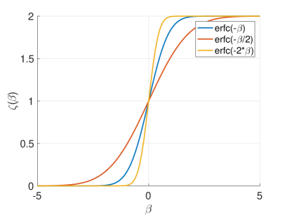
Figure 1: Plot of different choices of smoothly defined $\zeta=\zeta(\beta)$.

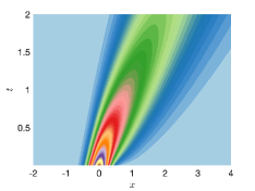
(a) $\zeta(x)=\operatorname{erfc}(-\frac{x}{2})$

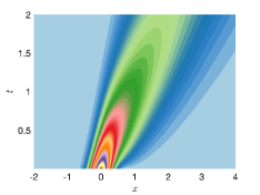
(b) $\zeta(x)=\operatorname{erfc}(-x)$

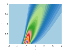
(c) $\zeta(x)=\operatorname{erfc}(-2x)$

Figure 2: Wave propagation corresponding to different choices of smooth $\zeta=\zeta(x)$ with a smooth initial data: top view.

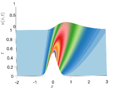
(a) $\zeta(x)=\operatorname{erfc}(-\frac{x}{2})$

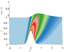
(b) $\zeta(x)=\operatorname{erfc}(-x)$

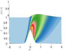
(c) $\zeta(x)=\operatorname{erfc}(-2x)$

Figure 3: Wave propagation corresponding to different choices of smooth $\zeta=\zeta(x)$ with a smooth initial data: zoom-in 3D view.

4.2.2 $\psi_{0}$ discontinuous, $\zeta$ smooth

Now, we consider the case where horizon parameter function $\zeta$ is smooth but the initial data $\psi_{0}$ is discontinuous, corresponding to the situation given in theorem 3.1. We can use the same numerical method as equation (2.2) to simulate the numerical solution of $[u]$.

Here we choose

$$H(s)=20e^{-10s^{2}},\quad\zeta(x)=\operatorname{erfc}(-x)$$

and

$$\psi_{0}(x)=\left\{\begin{array}[]{cc}\frac{1}{p},&-p<x<0\\ -\frac{1}{p},&0\leqslant x<p\\ 0,&\text{ otherwise, }\end{array}\right.$$

for some given parameter $p>0$.

Even though the simulations are carried out on a much larger spatial domain to ensure that the accuracy of the solutions are maintained with the domain truncation, we only plot part of the solutions for $x\in(-2,4)$ and $t\in(0,2)$ or $t\in(0,1)$. Likewise, we also carried out simulations for various values of $p$ but we present the case with $p=1$ mostly as the representative case. As comparisons, we also plot the solutions corresponding to the nonlocal model with a constant horizon parameter $\zeta(x)\equiv 0.1$ and the local limit (with $\zeta(x)\equiv 0$ effectively).

Figure 4 shows the top view of the numerical simulation results of $u$ for $p=1.0$ obtained using the numerical scheme (4.7) for $t\in(0,2)$, while Figure 5 gives the 3D view of the solutions for $t\in(0,1)$. The discontinuities of the initial data are at $x=0$ and $x=\pm 1$. For the nonlocal horizon function $\zeta(x)=\operatorname{erfc}(-x)$, we note that $\zeta(-1)$ is around $0.1573$, $\zeta(0)=1$ while $\zeta(1)$ is about $1.8427$. So the nonlocal effects are much stronger at $x=0$ and $x=1$. Indeed, the presence of stationary-in-time spatial discontinuities of the solutions can be captured by abrupt and sharp changes in color densities along vertical lines in the plots, see in particular Figure 4 (a) at $x=0$ and $x=1$ for most visible results. Since the jumps decay exponentially in time, the discontinuities eventually become unnoticeable. Nonlocal effects are less evident for smaller horizon function values, so that the stationary-in-time discontinuities would only be visible for a very short period of time, as one can see for $x=-1$ in Figure 4 (a). This can also be observed for all spatial positions in Figure 4 (b). On the other hand, for the local model, the discontinuities of the solutions travel along characteristic lines, and they maintain nearly the same magnitude, except for the dissipation due to numerical viscosity. These numerical results reported for this example are consistent with our analytical study in the previous section.

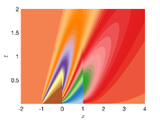
(a) $\zeta(x)=\operatorname{erfc}(-x)$

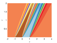
(b) $\zeta(x)\equiv 0.1$

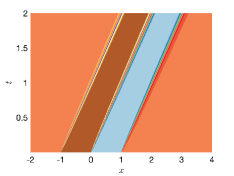
(c) $\zeta(x)\equiv 0$

Figure 4: Wave propagation with $\zeta(x)=\operatorname{erfc}(-x)$, $\zeta(x)\equiv 0.1$ and $\zeta(x)\equiv 0$ respectively: top view for $t\in(0,2)$.

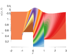
(a) $\zeta(x)=\operatorname{erfc}(-x)$

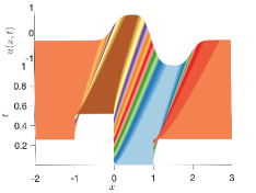
(b) $\zeta(x)\equiv 0.1$

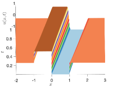
(c) $\zeta(x)\equiv 0$

Figure 5: Wave propagation with $\zeta(x)=\operatorname{erfc}(-x)$, $\zeta(x)\equiv 0.1$ and $\zeta(x)\equiv 0$ respectively: 3D view up to $t\in(0,1)$.

To highlight the propagation of singularities, In Figure 6 and 7, the time evolution of $\bm{[}u\bm{]}(x,t)$ are plotted at a given positions $x$ in different time intervals $(0,t)$ for different choices of horizon functions. The results are obtained by the two approaches mentioned in Section 4.1 are both presented to allow comparison and cross-validation. The blue curves in Figure 6 correspond to results obtained by the numerical evaluation of (3.2), while the red curves are obtained from the numerical solutions of equation (2.2), shown in the Figure 7.

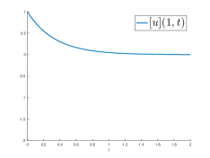
(a) $\zeta(x)=\operatorname{erfc}(-x)$

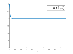
(b) $\zeta(x)\equiv 0.1$

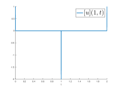
(c) $\zeta(x)\equiv 0$

Figure 6: Plot of $\bm{[}u\bm{]}(1,t)$ corresponding to different horizon up to $t\in(0,2)$ by method 4.1.2

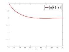
(a) $\zeta(x)=\operatorname{erfc}(-x)$

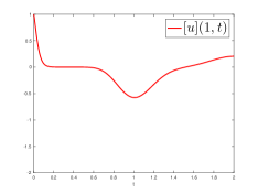
(b) $\zeta(x)\equiv 0.1$

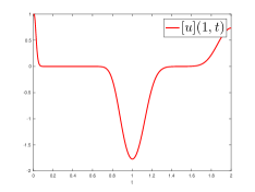
(c) $\zeta(x)\equiv 0$

Figure 7: Plot of $\bm{[}u\bm{]}(1,t)$ corresponding to different horizon up to $t\in(0,2)$ by method 4.1.1

From Figure 6 and Figure 7, we can find that the results obtained by the two methods are generally consistent with each other, up to the numerical viscous effect, and are consistent with the conclusion in the Theorem 3.1. In the nonlocal model, corresponding to $(a)$ in Figures 6 and 7, $\bm{[}u\bm{]}$ monotonically changes with $t$ to 0.

The plots in $(c)$ of Figures 6 and 7 correspond to the local model, It should be noted that (c) in Figures 6 draws the direct evaluation of $[u$], as obtained from the propagation along the characteristic line, while and the values of $[u$] in (c) of Figure 7 are obtained by calculating the jump given by the numerical solution, which is affected by the numerical dissipation. Still, we see that $\bm{[}u\bm{]}$ decays rapidly to 0 at $x=1$, due to the initial discontinuity at $x=1$ getting shifted over time, though a peak reappears later in time, due to the arrival of the initial discontinuity started at $x=0$ at time 0.

In comparison, the plots of Figures 6(b) and 7(b) correspond to the solution of nonlocal model with a small constant horizon parameter. We can see the behavior of $\bm{[}u\bm{]}$ looks reasonably similar to the results of local model, because the influence of nonlocal effect is relatively weak, even though the nonlocal model shows more pronounced dissipation as expected. Indeed, the results reported in Figures 6(b) follow the theoretical estimate and reflect the fast decay of the initial discontinuity, while the results presented in Figures 7(b) are based on the numerical simulations and differentiations which get influenced later on in time by the reappearance of the sharper transitions (approximating the arrival of the initial discontinuity from $x=0$). In comparison, the results based on the evaluation of (3.2) is less affected by such effects of the numerical discretization.

4.2.3 $\psi_{0}$ piecewise smooth, $\zeta$ smooth

Now, we consider the case where horizon $\zeta$ is smooth but the initial data $\psi_{0}$ is piecewise smooth, corresponding to the situation given in theorem 3.2.

Here we choose

$$H(s)=20e^{-10s^{2}},\quad\zeta(x)=\operatorname{erfc}(-x)$$

and

$$\psi_{0}(x)=\left\{\begin{array}[]{cc}1-{|x|}/{p},&-p<x<p,\\ 0,&\text{ else, }\end{array}\right.\quad\text{for a given parameter}\;p>0.$$ (4.12)

We pick $p=0.5$ and $p=1$ for illustration. In Figure 8, we can see that the initial data $\psi_{0}(x)$ selected here is a continuous piecewise linear functions with different slopes. Its derivative has three discontinuities at $x=-1,0$ and $1$ with the one at $x=-1$ being in the local region. Thus, we mostly focus on the latter ones.

The results of the solutions on $x\in(-2,5)$ are shown in Figures 9 for $t\in(0,2)$ with a top view and Figures 10 for $t\in(0,1)$ (a zoomed-in version of Figure 9, with a 3D view) to illustrate the behavior of the solution. The visible ”vertical lines” appearing in the contours could signal potential singularities. However, as the colors on the two sides of a ”vertical line” have a much less dramatic transition, we can see that the lines are capturing the ”folds” in the solutions, that is, the discontinuities of $u_{x}$, as we expect. We can see the appearance of these ”folding lines” at $x=0$ and $x=p$. The initial Hat function gets smeared as time goes on, due to the dissipative effect present in the nonlocal equations. Also, as the changes of slopes in the initial data become larger (as $p$ gets smaller, from the right plot to the left plot), the folding line shows up more dramatically.

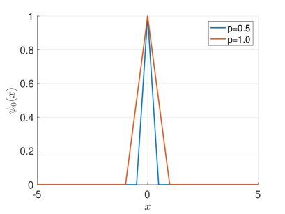
Figure 8: Plot of different choices of piecewise smoothly defined $\psi_{0}(x)$ for $x_{0}=0$

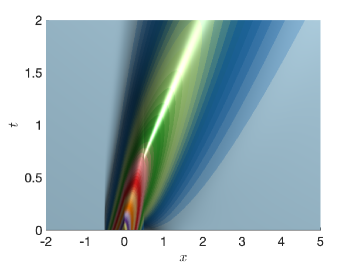
(a) $p=0.5$

(b) $p=1.0$

Figure 9: Wave propagation corresponding to different choices of $p$ for piecewise smooth initial data $\psi_{0}(x)$ with a smooth horizon: top view

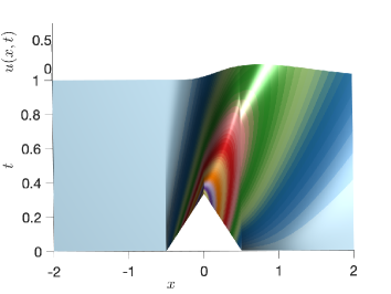
(a) $p=0.5$

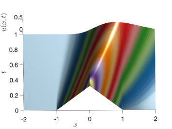
(b) $p=1.0$

Figure 10: Wave propagation corresponding to different choices of $p$ for piecewise smooth initial data $\psi_{0}(x)$ with a smooth horizon: zoom-in 3D view

In Figures 11 and 12, we plot the evolution of $\bm{[}u_{x}\bm{]}(x,t)$ in time for different horizon by the two numerical methods mentioned before. Results obtained from (3.6) correspond to the blue curves while red curves are from the jumps of difference quotients of numerical solutions. From Figures 11 and 12, we can find that $\bm{[}u_{x}\bm{]}$ monotonically diminishes to zero at $x=0$ and $x=p$ as described by equation (3.3), leading to consistent results obtained in the analytical estimates and numerical solutions in Figures 11 and 12. Moreover, comparing the plots in $(a)$ and $(c)$, and those in $(b)$ and $(d)$, among these figures, we can find that the results obtained by the two methods are basically the same, which is consistent with our expectations and helps to validate the numerical findings.

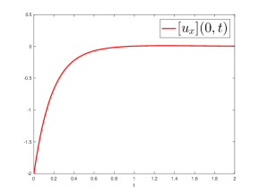
(a) $\bm{[}u_{x}\bm{]}(0,t)$ by method 4.1.1

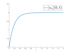
(b) $\bm{[}u_{x}\bm{]}(0,t)$ by method 4.1.2

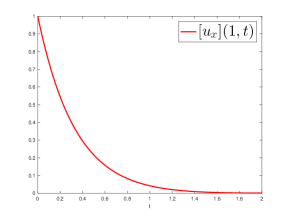
(c) $\bm{[}u_{x}\bm{]}(1,t)$ by method 4.1.1

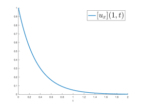
(d) $\bm{[}u_{x}\bm{]}(1,t)$ by method 4.1.2

Figure 11: Plots of $\bm{[}u_{x}\bm{]}(x,t)$ computed by different methods with $p=1$ and $x=0$ and $1$ for $t\in(0,2)$.

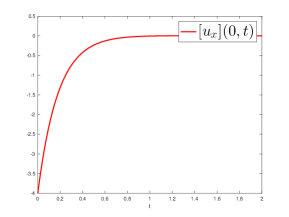
(a) $\bm{[}u_{x}\bm{]}(0,t)$ by method 4.1.1

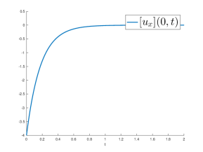
(b) $\bm{[}u_{x}\bm{]}(0,t)$ by method 4.1.2

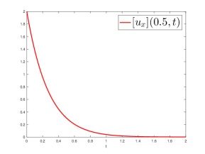
(c) $\bm{[}u_{x}\bm{]}(0.5,t)$ by method 4.1.1

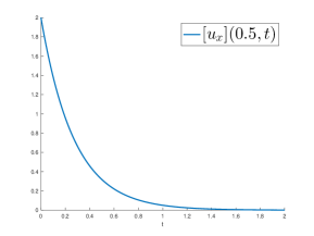
(d) $\bm{[}u_{x}\bm{]}(0.5,t)$ by method 4.1.2

Figure 12: Plots of $\bm{[}u_{x}\bm{]}(x,t)$ computed by different methods with $p=0.5$ and $x=0$ and $0.5$ for $t\in(0,2)$

4.2.4 $\psi_{0}$ smooth, $\zeta$ piecewise smooth

Now, we consider the case where initial data $\psi_{0}$ is smooth but the horizon $\zeta$ is piecewise smooth, corresponding to the situation given in Theorem 3.3. Here we choose

$$H(s)=20e^{-10s^{2}},\quad\psi_{0}(x)=e^{-10x^{2}}$$

and

$$\zeta(x)=\max\{\min\{kx,6\},0\},\quad\text{for}\;k=1,\;2\;\text{and}\;3\;\text{respectively}.$$ (4.13)

In Figure 13, we can see that the horizon $\zeta$ selected here is three piecewise smooth functions with transition layers becoming narrower as the slope $k$ changes from 1 to 2 then to 3. The jumps in the derivative $\zeta^{\prime}$ are at $x=0$ and $x=6/k$. While the latter is within the nonlocal region, the former is a local-nonlocal transition point. Thus, we may expect more evident jumps in the space derivative of the solution at $x=6/k$.

The results of the solutions on $x\in(-4,6)$ are shown in Figure 14 for $t\in(0,2)$ with a top view and Figure 15 for $x\in(-4,4)$ and $t\in(0,1)$ for a zoomed-in 3D view of Figure 14. The folding ”vertical line” appearing in the contours again are capturing the discontinuities of $u_{x}$, which in this case, are generated by the discontinuities in the horizon functions. The Gaussian peak in the initial data gets smeared as time goes on, due to the dissipative effect present in the nonlocal equations. Still, one can see that the smeared peak still travel largely along the local characteristics. A closer look shows that the smearing (dissipation) due to the nonlocal interactions gets more evident for larger $k$ (from the left plot to the right plot), which is consistent to the fact the nonlocal region expands with larger $k$, Moreover, the folding lines also become more evident (as indicated by more dramatic color changes shown in the plots).

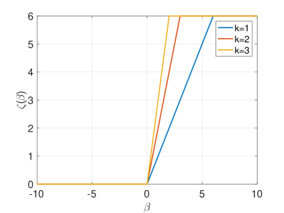
Figure 13: Plot of different choices of piecewise smoothly defined $\zeta=\zeta(\beta)$

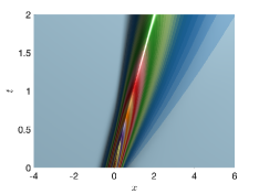
(a) $k=1$

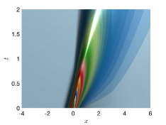
(b) $k=2$

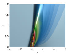
(c) $k=3$

Figure 14: Wave propagation corresponding to different choices of $k$ for piecewise smooth $\zeta=\zeta(x)$ with a smooth initial data: top view

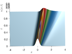
(a) $k=1$

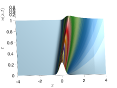
(b) $k=2$

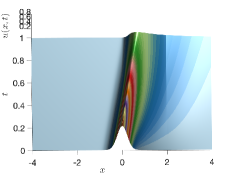
(c) $k=3$

Figure 15: Wave propagation corresponding to different choices of $k$ for piecewise smooth $\zeta=\zeta(x)$ with a smooth initial data: zoom-in 3D view

In Figure 16, we examine more closely the time evolution of $\bm{[}u_{x}\bm{]}(x,t)$ at $x=\frac{6}{k}$ for different horizon choices. We present the results computed by the direct evaluation of $\bm{[}u_{x}\bm{]}(x,t)$ using the method 4.1.2.

For different values of $k$, we can observe some consistent patterns. First, as predicted by the equation (3.3), with the smooth initial data, we can see that there is no jump initially in $u_{x}(\frac{6}{k},0)$. As $t>0$, $\bm{[}u_{x}\bm{]}(\frac{6}{k},t)$ starts to change with the overall magnitude gets larger for the case with a larger value of $k$. This can be seen from the equation (3.3), with the smooth initial data, we can see that $\bm{[}u_{x}\bm{]}(x,t)$ is proportional to the jump in $\zeta^{\prime}$. The latter is measured by $k$ for our example. As the initial smooth Gaussian peak gets smeared, it still travels along the characteristic lines which contributes to the more dramatic change in $\bm{[}u_{x}\bm{]}(\frac{6}{k},t)$ during the time when the peak passes through $x=\frac{6}{k}$ later in time, Overall, these observations are consistent to the patterns of the computed numerical solutions presented in Figures 14 and Figure 15.

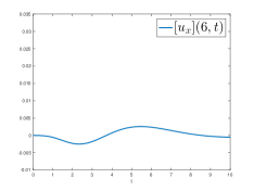
(a) $k=1$ and $x=6$

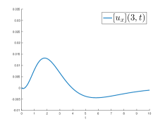
(b) $k=2$ and $x=3$

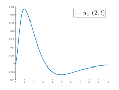
(c) $k=3$ and $x=2$

Figure 16: Plots of $\bm{[}u_{x}\bm{]}(x,t)$ computed by method 4.1.2 corresponding to different $k$ and $x$ up to $t\in(0,10)$

4.2.5 $\psi_{0}$ piecewise smooth, $\zeta$ piecewise smooth

Now, we consider the case where both the horizon $\zeta$ and the initial data $\psi_{0}$ are piecewise smooth. corresponding to the situation given in theorem 3.3.

Here we choose $H(s)=20e^{-10s^{2}}$, $\psi_{0}(x)$ is given by (4.12) with $p=0.5$, $1$ and $2$ respectively, and $\zeta$ is taken to be the same as (4.13), with $k=1$, $2$ and $3$ respectively.

In this case, according to the previous theorem, we expect that to see discontinuities in $u_{x}$ at locations where the derivative of either $\psi_{0}$ or $\zeta$ is discontinuous. The results of the solutions for $k=1$ and $p=0.5$ and $p=1.0$ on $x\in(-2,4)$ are shown in Figure 17 for $t\in(0,2)$ with a top view and Figure 18 for $t\in(0,1)$ with a 3D view to illustrate solutions. Similar results for $k=3$ and $p=2.0$ are presented in Figure 19 for $t\in(0,3)$ with both top and 3D views. Some folding ”vertical lines”, again for discontinuities of $u_{x}$ at $x=0$, $x=p$ and $x=\frac{6}{k}$, can be observed, which represent the stationary discontinuities in the spatial derivatives of solutions at those locations. Also, relatively speaking, larger $k$ and smaller $p$ would all make the jumps in the spatial derivatives more visible.

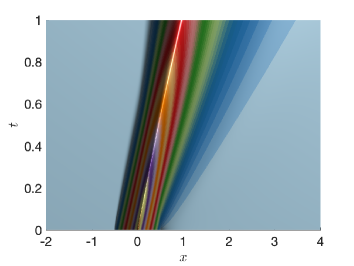
(a) $k=1,p=0.5$

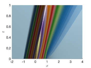
(b) $k=1,p=1.0$

Figure 17: Wave propagation corresponding to different choices of piecewise smooth $\zeta$ with a piecewise smooth initial data $\psi_{0}$: top view.

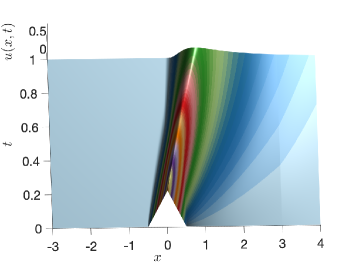
(a) $k=2,p=0.5$

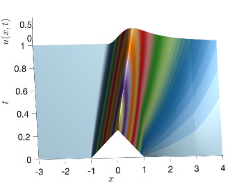
(b) $k=2,p=1.0$

Figure 18: Wave propagation corresponding to different choices of piecewise smooth $\zeta$ with a piecewise smooth initial data $\psi_{0}$: zoom-in 3D view.

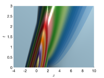
(a) top view

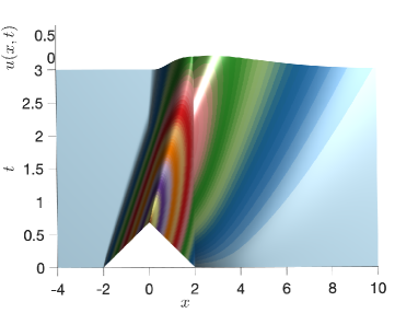
(b) 3D view

Figure 19: Wave propagation corresponding to different views of piecewise smooth $\zeta$ with a piecewise smooth initial data $\psi_{0}$ with $k=3$ and $p=2.0$.

To see the evolution of the jumps in $u_{x}$ in more details, we plot $\bm{[}u_{x}\bm{]}(x,t)$ in time for $x=p$ and $x=6/k$ corresponding to the cases with $x_{0}=0$, $p=1$ and $2$ for the initial data and $k=2$ and $3$ for the horizon function. We note that the behavior of discontinuity of $u_{x}$ at $x=0$ is more subtle, as it is caused by discontinuities of $\psi_{0x}$ and $\zeta^{\prime}$ and the additional fact that there is a transition from local ($\zeta=0$) to nonlocal ($\zeta>0$) regions at $x=0$. Note that with $\zeta(0)=0$, so (3.2) is technically not applicable at $x=0$. In the fully nonlocal region, we can use the method mentioned in Section 4.1.2 for the evaluation of the equation (3.2). The results are presented in the plots in in Figure 20,

From the plots in in Figure 20, we first look at the case $x=p=1$ with $k=2$, Here, $\bm{[}u_{x}\bm{]}(1,t)$ decays monotonically to 0, which is purely due to the discontinuity of $\psi_{0x}$, which is similar to the behavior observed for discontinuous initial data with a smooth horizon function,

Meanwhile for $p=1$ and $k=2$, at $x=\frac{6}{k}=3$, there is no jump of the derivative of the initial data at this location, so the generation of discontinuity in $u_{x}$ is controlled by $\zeta^{\prime}$. We see that $\bm{[}u_{x}\bm{]}(x,t)$ starts from zero and varies in time, and is influenced by the passing of the wave fronts, and the behavior is similar to those observed before in plots in Figures 16.

As for the case $k=3$ and $p=2$, we have the co-existence of jumps in $\psi_{0x}$ and $\zeta^{\prime}$ at both $x=0$ and $x=6/k=p=2$. Only $x=2$ is in the nonlocal region. We can observe the behavior from Figure 20 (c) is largely dominated by the jump of $\psi_{0x}$, yet the fast exponential decay is no longer observed due to the contributions of jumps of in $\zeta^{\prime}$, which makes the evolution different from ones observed earlier.

To summarize, similar to what are demonstrated in previous examples, results for this more example involving jumps in both $\psi_{0x}$ and $\zeta^{\prime}$ based on the estimates in Section 4.1.2 are consistent to those presented by the numerical solutions to the nonlocal models and also match well with the theoretical understanding.

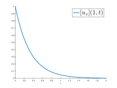
(a) $x=p=1.0$, $k=2$

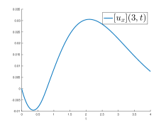
(b) $x=\frac{6}{k}$, $p=1.0$, $k=2$

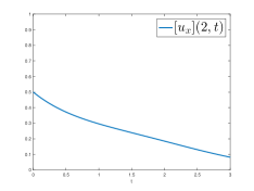
(c) $x=p=2.0=\frac{6}{k}$, $k=3$

Figure 20: Plots of $\bm{[}u_{x}\bm{]}(x,t)$ at different spatial locations for various values of $p$ and $k$.

5 Conclusion

Understanding the phenomenon of singularity propagation is of particular interests in mechanics and other physical processes. In this work, we focus on the study of singularity propagation in waves modeled by a nonlocal convection equation with variable nonlocal interactions. This new study complements an earlier study in [31] and gives a deeper understanding both theoretically and computationally. There are still many issues to be further investigated in the future. For example, one may conduct more careful studies related to the wave dispersion and reflection due to the variations in the horizon parameter, as pursued in other recent studies [21, 23]. The effect of boundary conditions is also an interesting problem worthy further investigation. Naturally, the one-dimensional linear problem is just one of the simplest examples, and for more practical and complex applications, we need to consider nonlinear and high-dimensional problems in future studies.

Declarations

Data Availability

The datasets generated during the current study are available from the corresponding author on reasonable request. They support our published claims and comply with field standards.

Competing of interest

The authors declare that they have no known competing financial interests or personal relationships that could have appeared to influence the work reported in this paper.

Funding

Research of Yan Xu is supported by NSFC grant No. 12071455. Research of Qiang Du is supported by NSF DMS-2012562.

Authors’ contributions

All authors contributed to the study conception and design. Material preparation, data collection and analysis were performed by Xiaoxuan Yu. The first draft of the manuscript was written by Xiaoxuan Yu and all authors commented on previous versions of the manuscript. All authors read and approved the final manuscript

Acknowledgements

The authors would like to thanks Jiwei Zhang for helpful discussions on the subject.

Financial disclosure

None reported.

References

- [1] Debora Amadori and Wen Shen. An integro-differential conservation law arising in a model of granular flow. Journal of Hyperbolic Differential Equations, 9(01):105–131, 2012.
- [2] Peter Bates and Adam Chmaj. An integrodifferential model for phase transitions: Stationary solutions in higher space dimensions. Journal of Statistical Physics, 95:1119–1139, 06 1999.
- [3] Fernando Betancourt, Raimund Bürger, Kenneth H Karlsen, and Elmer M Tory. On nonlocal conservation laws modelling sedimentation. Nonlinearity, 24(3):855, 2011.
- [4] Bartomeu Coll and Jean-Michel Morel. Image denoising methods. a new nonlocal principle. SIAM Review, 52:113–147, 03 2010.
- [5] Rinaldo M Colombo, Francesca Marcellini, and Elena Rossi. Biological and industrial models motivating nonlocal conservation laws: A review of analytic and numerical results. Network and Heterogeneous Media, 11(1):49–67, 2016.
- [6] Marta D’Elia, Xingjie Li, Pablo Seleson, Xiaochuan Tian, and Yue Yu. A review of local-to-nonlocal coupling methods in nonlocal diffusion and nonlocal mechanics. Journal of Peridynamics and Nonlocal Modeling, 2021, to appear. https://doi.org/10.1007/s42102-020-00038-7
- [7] Qiang Du. Nonlocal Modeling, Analysis, and Computation. Society for Industrial and Applied Mathematics, Philadelphia, PA, 2019.
- [8] Qiang Du, Zhan Huang, and Philippe G LeFloch. Nonlocal conservation laws. a new class of monotonicity-preserving models. SIAM Journal on Numerical Analysis, 55(5):2465–2489, 2017.
- [9] Qiang Du, Zhan Huang, and Richard B Lehoucq. Nonlocal convection-diffusion volume-constrained problems and jump processes. Discrete & Continuous Dynamical Systems-B, 19(2):373, 2014.
- [10] Qiang Du, Xingjie Helen Li, Jianfeng Lu, and Xiaochuan Tian. A quasi-nonlocal coupling method for nonlocal and local diffusion models. SIAM Journal on Numerical Analysis, 56(3):1386–1404, 2018.
- [11] Qiang Du and Xiaochuan Tian. Heterogeneously localized nonlocal operators, boundary traces and variational problems. Proceedings of the Seventh International Congress of Chinese Mathematicians, Beijing, 1:217–236, 2016.
- [12] Qiang Du, Jiang Yang, and Zhi Zhou. Analysis of a nonlocal-in-time parabolic equation. Discrete and continuous dynamical systems, 22(2):339–368, 2017.
- [13] Qiang Du, Jiwei Zhang, and Chunxiong Zheng. Nonlocal wave propagation in unbounded multi-scale media. Communications in Computational Physics, 24(4):1049–1072, 2018.
- [14] Marta D’Elia, Qiang Du, Max Gunzburger, and Richard Lehoucq. Nonlocal convection-diffusion problems on bounded domains and finite-range jump processes. Computational Methods in Applied Mathematics, 17(4):707–722, 2017.
- [15] Marta D’Elia, Mauro Perego, Pavel Bochev, and David Littlewood. A coupling strategy for nonlocal and local diffusion models with mixed volume constraints and boundary conditions. Computers & Mathematics with Applications, 71(11):2218–2230, 2016.
- [16] Guodong Fang, Shuo Liu, Maoqing Fu, Bing Wang, Zengwen Wu, and Jun Liang. A method to couple state-based peridynamics and finite element method for crack propagation problem. Mechanics Research Communications, 95:89–95, 2019.
- [17] Ugo Galvanetto, Teo Mudric, Arman Shojaei, and Mirco Zaccariotto. An effective way to couple fem meshes and peridynamics grids for the solution of static equilibrium problems. Mechanics Research Communications, 76:41–47, 2016.
- [18] Simone Göttlich, Simon Hoher, Patrick Schindler, Veronika Schleper, and Alexander Verl. Modeling, simulation and validation of material flow on conveyor belts. Applied mathematical modelling, 38(13):3295–3313, 2014.
- [19] Kuang Huang and Qiang Du. Stability of a nonlocal traffic flow model for connected vehicles. arXiv preprint arXiv:2007.13915, 2020.
- [20] Michiya Imachi, Takaaki Takei, Murat Ozdemir, Satoyuki Tanaka, Selda Oterkus, and Erkan Oterkus. A smoothed variable horizon peridynamics and its application to the fracture parameters evaluation. Acta Mechanica, 232(2):533–553, 2021.
- [21] Xingjie Li and Pablo Seleson. A study of generating nonlocal wave. Preprint, 2021.
- [22] Jaber Nikpayam and Mohammad Ali Kouchakzadeh. A variable horizon method for coupling meshfree peridynamics to fem. Computer Methods in Applied Mechanics and Engineering, 355:308–322, 2019.
- [23] Hayden Pecoraro, Kelsey Wells, Xingjie Li, and Pablo Seleson. A study of dispersion relations for coupling nonlocal and local elasticities. Preprint, 2021.
- [24] Stewart Silling, David Littlewood, and Pablo Seleson. Variable horizon in a peridynamic medium. Journal of Mechanics of Materials and Structures, 10(5):591–612, 2015.
- [25] Stewart A Silling and Richard B Lehoucq. Peridynamic theory of solid mechanics. In Advances in applied mechanics, volume 44, pages 73–168. Elsevier, 2010.
- [26] Yunzhe Tao, Xiaochuan Tian, and Qiang Du. Nonlocal models with heterogeneous localization and their application to seamless local-nonlocal coupling. Multiscale Modeling & Simulation, 17(3):1052–1075, 2019.
- [27] Hao Tian, Lili Ju, and Qiang Du. Nonlocal convection–diffusion problems and finite element approximations. Computer Methods in Applied Mechanics and Engineering, 289:60–78, 2015.
- [28] Xiaochuan Tian and Qiang Du. Trace theorems for some nonlocal function spaces with heterogeneous localization. SIAM Journal on Mathematical Analysis, 49(2):1621–1644, 2017.
- [29] Xiaonan Wang, Shank S Kulkarni, and Alireza Tabarraei. Concurrent coupling of peridynamics and classical elasticity for elastodynamic problems. Computer Methods in Applied Mechanics and Engineering, 344:251–275, 2019.
- [30] Olaf Weckner and Rohan Abeyaratne. The effect of long-range forces on the dynamics of a bar. Journal of the Mechanics and Physics of Solids, 53(3):705–728, 2005.
- [31] Xiaoxuan Yu, Yan Xu, and Qiang Du. Asymptotically compatible approximations of linear nonlocal conservation laws with variable horizon. Numerical Methods for Partial Differential Equations, 2021, to appear. https://doi.org/10.1002/num.22849