Machine-Learning enabled analysis of ELM filament dynamics in KSTAR

Abstract

The emergence and dynamics of filamentary structures associated with edge-localized modes (ELMs) inside tokamak plasmas during high-confinement mode is regularly studied using Electron Cyclotron Emission Imaging (ECEI) diagnostic systems. ECEI allows to infer electron temperature variations, often across a poloidal cross-section. Previously, detailed analyses of filamentary dynamics and classification of the precursors to ELM crashes have been done manually. We present a machine-learning-based model, capable of automatically identifying the position, spatial extend, and amplitude of ELM filaments. The model is a deep convolutional neural network that has been trained and optimized on an extensive set of manually labeled ECEI data from the KSTAR tokamak. Once trained, the model achieves a $93.7\%$ precision and allows to robustly identify plasma filaments in unseen ECEI data. The trained model is used to characterize ELM filament dynamics in a single H-mode plasma shot. We identify quasi-periodic oscillations of the filaments size, total heat content, and radial velocity. The detailed dynamics of these quantities appear strongly correlated with each other and appear qualitatively different during the pre-crash and ELM crash phases.

Cooper Jacobusa cjacobus@berkeley.edu Minjun J. Choib Ralph Kubec

aUniversity of California, Berkeley, CA 94720, USA bKorea Institute of Fusion Energy, Daejeon 34133, Republic of Korea cPrinceton Plasma Physics Laboratory, NJ 08540, USA

Machine Learning Convolutional Neural Networks Edge Localized Mode Electron Cyclotron Emission Imaging

1 Introduction

High confinement mode (H-mode) plasmas are characterized by a steep density gradient in the edge, the so-called pedestal region, of the confined plasma. Access to H-mode is achieved by plasma heating and once a critical heating threshold is exceeded the pedestal typically forms within a few milliseconds. Associated with this rapid transition are strong, sheared electric drifts, localized to the pedestal region, as well as a local suppression of local turbulent fluctuations [1, 2, 3]. These sheared electric drifts form a transport barrier which inhibits radial transport. As a result, the energy confinement properties of H-mode plasmas are superior to those in low-confinement mode and render this mode of operation an attractive baseline scenario for ITER [4, 5]. Edge localized modes (ELMs) are a ubiquitous feature of H-mode plasmas. They cause an intermittent relaxation of the edge pressure gradient, caused by so-called ELM crashes. During these violent events, plasma ejects from the confined region onto material surfaces of the vacuum vessel. Upon contact with the hot plasma, material surfaces erode and sputtered wall atoms contaminate the confined plasma. These phenomena are at the core of complex research activities in the fusion community.

There are various types of ELMs, identified based on periodicity and dependence on heating power. These types include violent, low-frequency Type-I ELMs, or more intermittent, burst-like Type-III ELMs, as well as a mixed regime [6, 7, 8]. While two-fold stability analysis of peeling-ballooning modes explains linear stability of ELMs [9, 10], the actual ELM crash is a nonlinear magnetohydrodynamic phenomenon and an area of active research interest [11, 3, 12, 13, 10, 14].

At the KSTAR Tokamak, a two-dimensional (2D) Electron Cyclotron Emission imaging diagnostic [15, 16] has been used to investigate the nonlinear dynamics of ELMs, including their explosive growth, saturation, and crash [17, 18]. In the 2D ECE images, the ELM mode appears as a filamentary structure of the normalized temperature fluctuation near the pedestal top. The evolution of these ELM filaments is divided into three phases. During an initial growth phase, the amplitude of the mode structure increases while the structure itself rotates counterclockwise through the ECEI field of view. Once saturated, the ELM filament amplitude appears to stagnate while the filaments into finger-like structures that extend from the pedestal into the open field-line region. A similar phenomenology is reported from other tokamaks [19, 20, 21]. In order to investigate physical mechanisms that drive ELM filament dynamics and lead up to ELM crashes it is desirable to robustly estimate properties of the structures visible in the ECEI data. This includes for example the number of visible filaments, their amplitude, their spatial extent, and their velocities. With this information at hand, one can investigate all three phases, initial growth, saturation, as well as the ELM crash itself. This work introduces a machine-learning based model that allows automatic frame-by-frame detection of filamentary structures associated with ELMs. We do not distinguish between the turbulent inter-ELM phase and the non-linear evolution of the actual ELM crash. For a recent experimental review, the interested reader is referred to [22].

Given its ability to learn complex non-linear relations from large amounts of data, machine learning is applied to various tasks in fusion energy research. A major area of concern for developing magnetic confinement based fusion reactors is the safe shutdown of pulses before explosive disruptions exert intolerable stresses on plasma facing components. Besides disruption detection, it is a major goal to integrate machine-learning based detection algorithms into real-time plasma control systems in order to enable robust plasma control solutions [23, 24, 25, 26, 27, 28, 29, 30, 31, 32, 33, 34]. Reduced, or surrogate models are another successful use case of machine learning models in fusion energy sciences. Such models allow to instantaneously infer predictions of high-fidelity models for a given set of inputs. Surrogate models are for example relevant for complex optimization loops and similar integrated data analysis tasks. Post-shot analysis of plasma pulses for example can be performed orders of magnitude faster using surrogate models while retaining high accuracy [35, 36, 37, 38, 39, 40, 41].

Convolutional neural network based models have been used to explore connections between bursting behaviour of the plasma boundary and solitary perturbations [42]. Filamentary structures, sometimes called blobs when discussing scrape-off layer plasmas, present a ellipsoid footprint when viewed in the poloidal - radial plane [43]. Automatic detection of such structures is often been performed using blob detection, which identifies coherent structures of a minimum size that exceed a heuristically determined amplitude threshold [44, 45, 46]. Other work approaches blob detection using methods based on cross-correlation of spatial channels [47] or spatial displacement estimation [48]. Only recently have machine learning methods been used to identify the extent of filament structures in fusion plasmas [49]. Machine-learning based models learn detection criteria based on labeled training data. That is, they don’t require a-priori heuristically tuned parameters for structure detection but replace them with information encoded in expert-labeled training data. The approach presented here is of the same spirit and to the best knowledge of the authors a first attempt to use a machine-learning-based algorithm to investigate ELM filament dynamics.

The remainder of the article is structured as follows. In section 2 we introduce the used deep convolutional neural network architecture and describe its application for ECEI data. We also describe the developed training data set and the performance of the trained network on training and validation data sets. In section 3 we use the trained model to identify filamentary structures in a H-Mode plasma shot and explore their dynamical properties. We discuss the results and set them into context with other recent work in 4. A conclusion and directions for future work are given in 5

2 Machine learning detection of ELM filaments in ECEI data

Cyclotron radiation emission from free electrons in magnetically confined plasmas are routinely measured for diagnostic purposes [15, 50]. At KSTAR, 2D ECEI systems are used to measure electron temperature fluctuations $\delta T_{\mathrm{e}}/\langle T_{\mathrm{e}}\rangle$ over a two-dimensional field of view aligned in the poloidal cross-section on a microsecond timescale. [15, 16]. Each system covers rectangular cross-sections of the plasma with 24 by 8 pixels in the vertical and radial direction respectively, featuring aspatial resolution $2\mathrm{cm}$ and a sampling time of $2\mu\mathrm{s}$. In practice, the low-field side field-of-view extends about $40\,\mathrm{cm}$ vertically and about $10\,\mathrm{cm}$ radially which readily allows to visualize filamentary structures associated with ELMs.

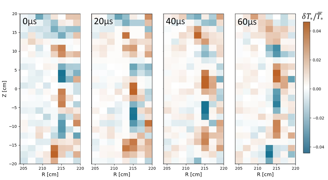
Figure 1: A sequence of ECE images taken during the initial growth phase of an ELM. Humans readily identify a modal structure with peaks and troughs which rotates counter-clockwise in this image sequence.

Normalizing to vanishing mean, the emission intensity sampled by the ECE diagnostic can be interpreted as a temperature fluctuation $\delta T/\langle T\rangle$. The temperature corresponds to the radiation temperature and it is usually justified to associate it with the electron temperature [15, 50]. All ECEi data used in this contribution is normalized this way, while pixels with low signal-to-noise ratio are replaced by a linear interpolant. The data was furthermore subject to a bandpass filter of $5-9\mathrm{kHz}$, the range being estimated as to capture the dominant fluctuations in between ELM crashes shown in Fig. 8. Figure 1 shows a sequence of bandpass filtered and normalized ECEI images that capture a mode structure associated with an ELM. To estimate the dynamics present in this sequence of images we can visually identify individual peaks and troughs in each image. Asserting that peaks (or troughs) in subsequent images with maximal overlap correspond to the same part of the observed mode structure, we estimate a rotation velocity of approximately $2\,\mathrm{cm}$ per $20\mu\mathrm{s}$ frame, that is, the modal structure rotates at roughly $1\mathrm{km}/\mathrm{s}$. A computer vision algorithm can automatically perform this calculation. For this, a detector should identify individual peaks in a single frame. Then a tracking algorithm can be used to track these peaks across a squence of images.

In this contribution, we use a Scaled-YOLOv4 (You Only Look Once) model [51, 52, 53] to identify ELM filaments in ECEI data. YOLO is a widely used class of object detection models and the Scaled-YOLOv4 model modifies the original YOLO architecture in order to be applicable to smaller images. Object detection models, such as YOLO, perform multi-class object detection on image data by outputting bounding box dimensions as well as a probability of belonging to a given class for each identified object. The YOLO model is based on a convolutional neural network (CNN) architecture, which applies a sequence of learned filters, each followed by non-linear activation functions, to input data. The size and the stride as well as the number of output channels of the convolution filters are fixed while the convolution matrix coefficients are trainable parameters. Besides its convolutional architecture, design choices in the YOLO architecture are made in order to optimize inference speed, which makes it one of the fastest image detection algorithms available [52]. YOLO models also perform exceptionally well, for example it has been found that they detect approximately three times fewer false positives than alternative architectures [54].

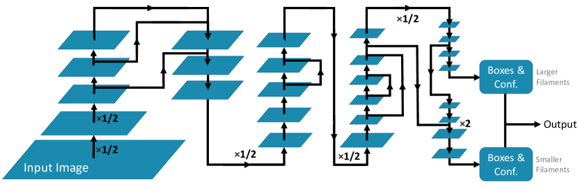
Figure 2: Illustration of the convolutional architecture implemented by the used YOLOv4 model. Blue rectangles denote data at a given layer and their size is proportional to the matrix dimensions. Black arrows denote connections between layers, and are annotated by scale factors in the case where a convolution changes the layer size. There are two outputs layers, each of the giving a set of bounding boxes as well as a confidence score for detected instances of object classes in the input image.

Figure 2 illustrates the architecture of the used Scaled YOLOv4 network. The input is a 192-by-64 pixel image with 3 channels. To transform the normalized $24\times 8$ ECEI data frames to this size they are up-sampled using cubic interpolation and then a colormap is applied. The first convolution applies a set of $32$ filters, each of size $3\times 3\times 3$ using a stride of 2 and outputs $32$ $92\times 32$ matrices, reducing the input resolution by a factor of 2. The values of these filters are the trainable parameters of the model. The output of the first layer consists of convolutions of the input image with each one of these 32 filters. The resulting stack of matrices is then used as input to the next layer. These 32 matrices are ’feature maps’ which represent the qualitative properties of a local neighborhood of pixels [55, 56]. Layers of these convolutions are applied to produce more specific feature maps until it is able to recognize complex features like filaments [57]. While connections are mostly between successive layers, YOLO also uses a number of residual connections, where the outputs of non-consecutive layers are concatenated along the channel dimension. The outputs of the YOLO network are two sets of bounding boxes with associated confidence scores. The first set of outputs is used to identify larger structures. Then, continuing processing through some more up-convolution layers, another output is generated that aims to identify smaller structures. Reference [52] describes the architecture in detail. For the work presented in this article we used the scaled YOLO-v4 implementation provided here .

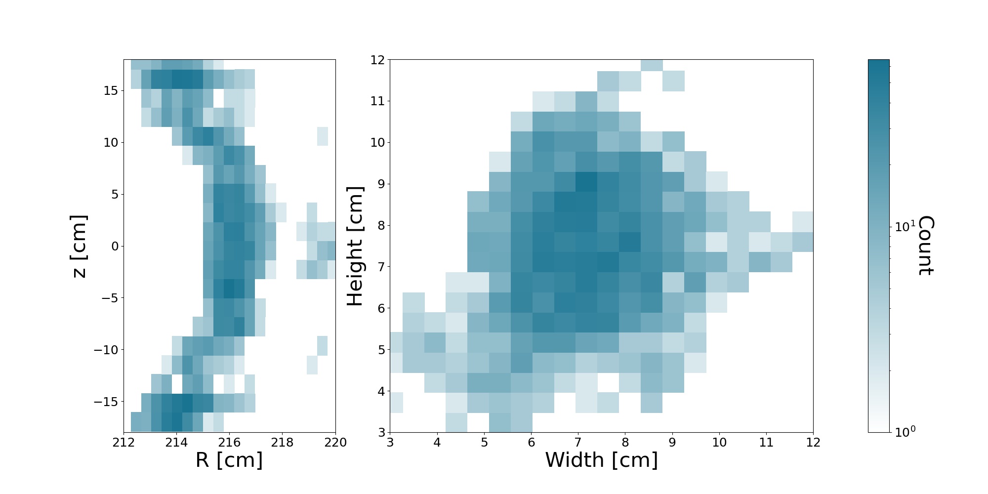
Figure 3: Histograms of the anchor and dimensions of the bounding boxes prescribed in the manually labelled training data.

YOLO is trained in a supervised fashion and requires labeled training data. We manually created a training set of ELM filaments by randomly selecting 1000 ECEI data frames from a single KSTAR shot and fit tight bounding boxes around ELM filaments that appear in these frames. A bounding box is described by four values: an anchor point in the 2d ECEI view, a width, and a height. We only label hot filaments which contain excess heat and therefore all bounding boxes are assigned the same class. Figure 3 shows the distribution of bounding boxes in the training set. The anchors appear mostly on a singular flux surfaces with some detections also at $R\approx 220\mathrm{cm}$ and $Z\approx 0\,\mathrm{cm}$. The width and height of the bounding boxes distribution in the manually labeled data are approximately $7\pm 3\mathrm{cm}$. There are only a few outliers in the bounding box size distributions, either centered at smaller sizes or tall filaments with a width of approximately $10\,\mathrm{cm}$ and a height of approximately $7\mathrm{cm}$.

The scope of this paper is intended to be an analysis of a single KSTAR shot, all frames included in the training data are from the range 2.6-2.8 seconds. The frames used for labeling were drawn from a uniform distribution. So they represent the temporal distribution of pre-growth, mid-growth, saturated, and mid-crash phases. On average, there is about $200\mathrm{\mu s}$ between any two frames, long enough that each there is negligible correlation between any two frames of the training set.

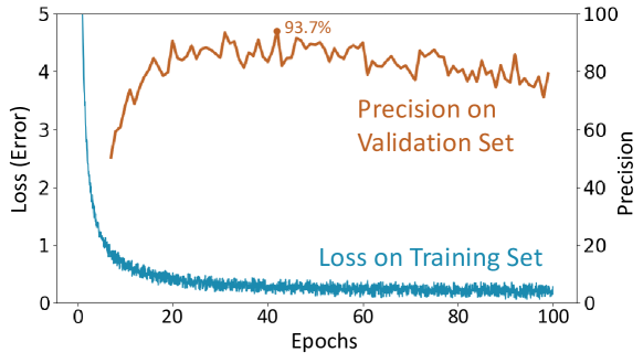
Figure 4: Calculated values of YOLO loss on the training set and precision on the validation set during training.

The task of the trained model is to output tightly fitting bounding boxes around ELM filament instances in unseen data. YOLO uses a special loss function which is given by a weighted sum of multiple terms. These include a binary cross-entropy term for correct instance labeling as well as a term describing intersection-over-union (IoU) misalignment of the bounding boxes. Intersection over union is a commonly used quantity in object identification and localization [52]. Given two boxes, IoU is calculated as the ratio over the intersection of the boxes to the union. For training, we randomly split the manually labeled data into a training set and a validation set, consisting respectively of 800 and 200 frames with their associated bounding boxes. The model parameters are optimized by minimizing the YOLO training loss function calculated over the training set for 100 epochs. We used a batch size of 64 randomly shuffled images and the Adam optimizer [58] with a learning rate of 0.00261, as recommended in the documentation of the used YOLOv4 implementation .

Performance metrics of the model can readily be calculated from its IoU predictions. To aid in consuming the IoU information, it is common to identify a detection where $IoU\geq 0.5$ as a true positive. Similarly, a false positive detection is an instance where $IoU<0.5$. A false negative detection is a case where the model identifies an object instance in an image where it is not present. And finally, a true negative detection is a case where the model does not identify object instances and they are not present in the image. During training, the performance of the model is monitored by tracking the value of the loss function calculated over the training set and the precision, the ratio between true positives to the sum of true and false positives, calculated on the validation set. Figure 4 shows the training loss and validation precision of our model during training. Initially, the training loss decreases sharply and flattens after about 40 iterations. At the same time, the precision on the validation set increases from about 50 to over $90\%$ from epoch 10 to 40.

After 42 epochs of training, the model achieves a $93.7\%$ precision on the validation set. That is, it correctly captures the bounding box of the majority of the validation data. It also achieves a $85.2\%$ recall on epoch 42, the ratio of true positives to the sum of true positives and false negatives. In other words, almost all detected filaments are indeed filaments present in the validation set. Training for more than 42 epochs we observe that the model begins to over-fit on the training set. On average, our model achieves $67.9\%$ IoU, which highlights that there is still notable disagreement between the two. This stems however mostly from misalignment of the bounding boxes and not from mis-detection of filaments. The model state reached in epoch 42 is used for inference.

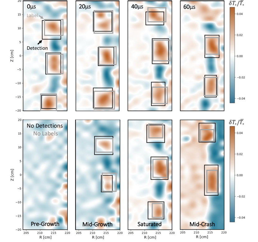
Figure 5: Examples of ELM filament detection in ECEI images, performed by a trained YOLO model. The upper row corresponds to the images in figure 1 and the lower row corresponds to images during various stages in an ELM crash. Gray boxes denote manually labelled objects and black boxes denote predictions from the YOLO model. (This figure is an illustration, there is usually much more time between training images.)

Figure 5 presents ELM filaments detected by the trained YOLO model. The upper row shows ECEI data frames shown in 1, but up-sampled to 192x96 pixels. The images shown in the lower row are taken from various phases of an observed ELM crash. The gray boxes denote manually labeled bounding boxes and predictions from the trained YOLO model are illustrated by black boxes. Visually inspecting the predictions we find that the center of the bounding boxes and their spatial extent corresponds well to the manual labels. During the saturated and the mid-crash phases, however, they appear to be more misaligned. The video supplementing this article further demonstrates the developed filament detection and tracking method applied to a $10\,\mathrm{ms}$ long time window.

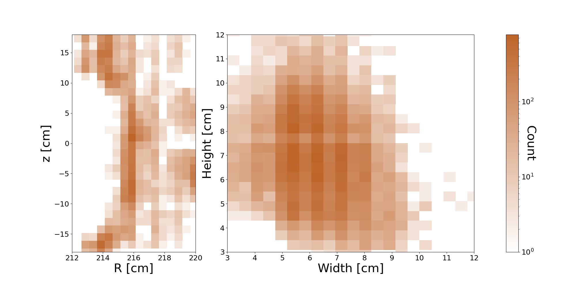
Figure 6: Histograms of the anchor and dimensions of the bounding boxes discovered by the trained machine learning model in the entire analyzed dataset.

To investigate what degree of confidence is warranted in the predictions made by the trained YOLO model we plot histograms of the spatial distribution of the detection boxes on unseen data in figure 6 below. We find that the distribution of anchor points now extends radially out over a single flux surface. Since CNNs are equivariant under translation this alone warrants no loss of confidence in the predicted bounding boxes. But we furthermore observe that the distribution of bounding box dimensions exceeds those prescribed in the training data. Detected bounding boxes of smaller width and height, between $3$ and $5\,\mathrm{cm}$ are frequently predicted but are absent in the training data. Since CNNs are not scale-invariant, these may be indicative of lower model performance for tall and skinny or short and broad boxes. Examples of this can be seen in Fig.5 in the mid-growth and mid-crash frames, where tall and skinny predicted bounding boxes appear to feature lower IoU than predicted bounding boxes that appear more square-like.

Besides filament detection, the output of the trained YOLO model can be used to compile derived measurements, such as an average filament amplitude, ⟨A⟩.

$$\langle A\rangle=\frac{1}{N}\sum_{n=1}^{N}A_{n}\textrm{ where }A_{n}=\sum_{i,j\in\mathrm{\textrm{bbox n}}}\left(\frac{\delta T}{\langle T\rangle}\right)_{i,j}^{+}.$$ (1)

This is approximately related to the average excess heat of all ELM filaments in a given ECEI frame. Here $i$ and $j$ index individual image pixels within a given bounding box and ⁺ indicates that this calculation considers only positive-valued pixels, ignoring negative-valued pixels sometimes found in the corners of the bounding boxes.

Filament motion is tracked by connecting bounding boxes of filaments detected in subsequent frames with one another. In particular, bounding boxes in consecutive frames with centers within 2cm of each other are taken to be the same filament. This method is applied to a series of frames by first identifying filaments in all frames. Then, starting at the first frame, identified filaments are associated with filaments from successor frames. Then their radial and poloidal velocity is estimated using the center of the bounding box. If no successor filaments can be identified, no velocity is calculated. We note here that the calculated filament velocities include contributions from background electric drifts. While these can readily be removed by calculating the radial electric field from a force balance model, here we focus only on properties of the filament tracking method developed. By detecting only peaks we do not assume any modal structure is present in the ECEI images. This allows us to calculate filament amplitude statistics in all parts of the ELM crash development, from pre-growth to the final ELM crash.

3 Data Analysis

In the following, we use the trained YOLO model to investigate ELM filament dynamics for one H-mode plasma in KSTAR. This shot features a toroidal magnetic field given by $B_{\mathrm{T}}=1.8\mathrm{T}$ and was neutral beam heated. Figure 7(a) shows time traces of the MHD energy, the emitted $D_{\mathrm{\alpha}}$ radiation, the plasma current, and the neutral beam power for shot 22289. The confined energy decreases and sharp peaks of the measured $D_{\alpha}$ radiation indicate the presence of ELMs. The peaking frequency of $D_{\alpha}$ and the plasma current $I_{\mathrm{p}}$ appear correlated while the neutral beam power remains approximately constant over the shown time slice. Figure 7(b) shows the magnetic equilibrium for this time slice, calculated using the EFIT [59] module in OMFIT [60]. The brown rectangle denotes the field of view of the ECEI diagnostic viewing the low-field side for which we report data analysis in the following.

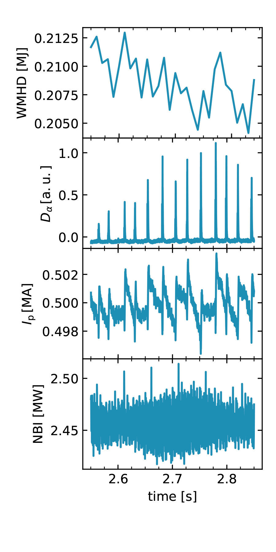
(a) Time traces of global plasma quantities.

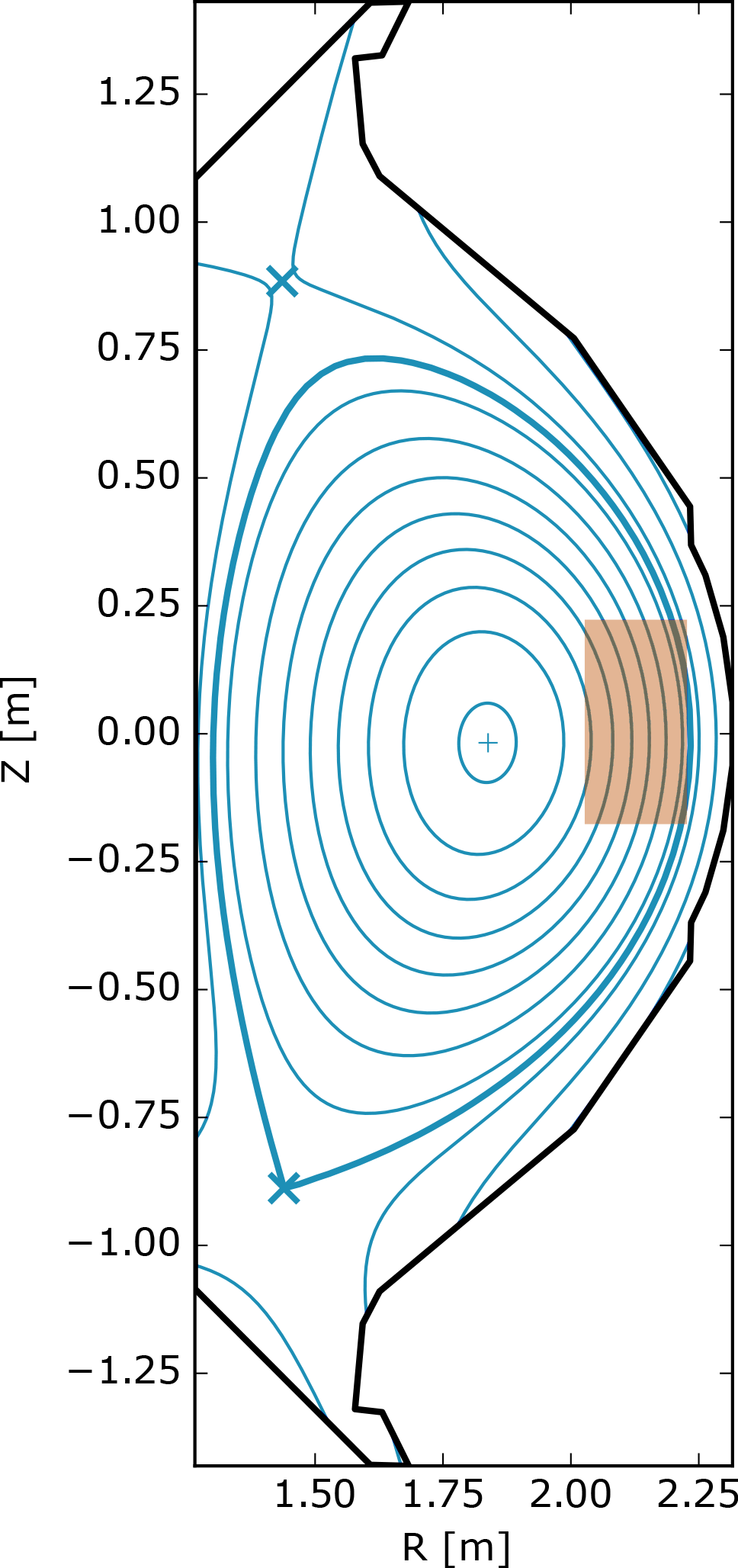
(b) Magnetic equilibrium reconstruction, he orange rectangle denotes the view of the ECEI diagnostic.

Figure 7: Global plasma state and magnetic equilibrium reconstruction for shot 22289

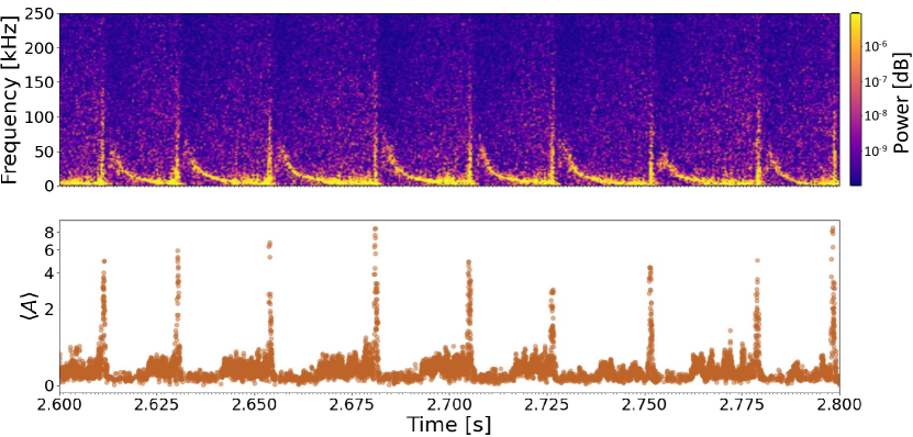
Figure 8: Spectrogram calculated using a single ECEi channel and evolution of $\langle A\rangle\>$.

As a first step, we investigate how the average filament amplitude $\langle A\rangle\>$, defined in Eq.(1), behaves during ELM cycles. Figure 8 shows the time series of the spectrogram, calculated from ECEI data, together with the evolution of $\langle A\rangle\>$. Here, ELM crashes appear as short bursts of broadband fluctuation in the spectrogram. In the inter-ELM crash period, the ELM mode appears as a coherent fluctuation in the spectrogram and its frequency decreases with the pedestal recovery. Similarly, $\langle A\rangle\>$also peaks during the ELM crash. The time evolution of $\langle A\rangle\>$, which is carried by detected filaments, can visually be divided into three states. Immediately after an ELM crash, $\langle A\rangle\>$is approximately zero. The extent of this state appears to overlap with the frequency decreasing (pedestal recovery) period in the spectrogram in which the ELM amplitude may be too small to be detected clearly. After this phase, $\langle A\rangle\>$exhibits a larger mean and fluctuations. This phase extends approximately over the same time intervals where only slow frequencies below about $10\,\mathrm{kHz}$ appear in the spectrogram and precedes the ELM crash. During the actual ELM crash, $\langle A\rangle\>$sharply peaks to values up to $5-10$, which is about two orders of magnitude larger than in the quiescent period that immediately follows the crash.

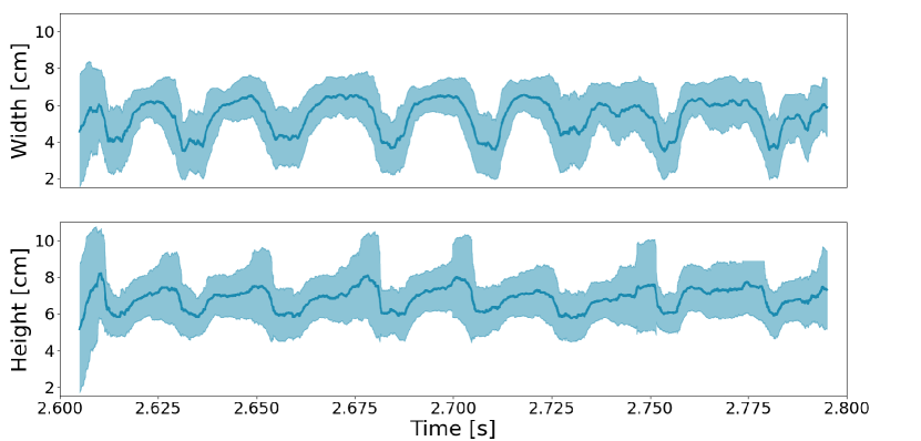
Figure 9: Width and height of detected filaments, calculated using a $0.01\,\mathrm{s}$ wide moving average window. The shaded area centered around the moving average denotes the moving standard deviation.

Figure 9 shows time-traces of the average bounding box width and height for the detected filaments, calculated using a $10\,\mathrm{ms}$ long moving average window. The shaded area denotes the standard deviation, calculated over the same interval as used for the moving average. Both, the average width and height undergo quasi-periodic oscillations that are correlated with the ELM crashes shown in 8. In the pre-crash phases, we observe average filament widths and heights of approximately $6\,\mathrm{cm}$. About $1\,\mathrm{ms}$ before the ELM crash the average height of the mode increases abruptly while its average width starts to decrease slowly, indicating that a significant change of the mode aspect ratio resulted in the ELM crash (see Fig. 5). The appearance of the poloidally elongated mode just before the crash is consistent with the previous manual analysis [61] where it was identified as a solitary perturbation. After the ELM crash, the mode structures recover the pre-crash width and height. Figure 9 demonstrates that the machine-learning based model can be used to identify ELM filament sizes for the temporal evolution of the ELM dynamics, extending through multiple pre-crash, growth, and crash phases.

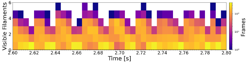
Figure 10: Histogram of detected filament count.

The average number of filaments detected in each frame, shown in Fig.10, shows similar quasi-periodic oscillations. Here the individual histograms are calculated over intervals of $5\,\mathrm{ms}$. For the pre-crash periods, the majority of frames feature zero to three filaments, but single frames show up to 5 detected filaments. During the ELM crash, the number of detected filaments decreases. Here, more frames are absent of any detected filaments and virtually no frames in this period have more than three detected frames. This is possibly due to an increased poloidal wavelength. During the crash-phase, there are many frames where large regions of the image are hot (see Fig 5) or where the amplitude of the background turbulence is comparable to filaments, which often confuses the model.

Figure 11: Amplitude dynamics of ELM filaments in the interval leading up to ELM crash.

Figure 11 shows the evolution of $\langle A\rangle\>$in a millisecond time interval right before ELM crashes. All four instances show short growth periods where the total amount of heat contained in the ELM filaments increases by a factor of $2-4$. These growth periods may be followed by a saturation period where $\langle A\rangle\>$varies only little. But we also observe that after a short growth phase, $\langle A\rangle\>$returns to its initial value. Then $\langle A\rangle\>$may immediately begin to grow again, as observed for $t=2.701\,\mathrm{s}$ or remain at a low value before growing again, as observed at $t=2.787\,\mathrm{s}$. The duration of the observed growth phases is about $1\,\mathrm{ms}$, regardless of whether $\langle A\rangle\>$saturates afterwards or not.

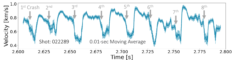
Figure 12: Moving average of poloidal filament velocity.

Figure 12 shows time series of the poloidal velocity.The ELM crash period is correlated with a sharp drop in poloidal filament velocity. In the intervals leading up to an ELM, for example between $t=2.615-2.63\,\mathrm{s}$ the poloidal velocity decreases slightly. While in other instances, for example during $t=2.66-2.68\mathrm{s}$, the poloidal velocity remains approximately constant. ELM crashes are associated with a rapid drop of the filaments poloidal velocity. In some instances, for example at $t=2.615\,\mathrm{s}$ the poloidal velocity immediately recovers to its pre-crash value while in other instances, for example at $t=2.655\,\mathrm{s}$, the poloidal velocity remains attenuated for a short interval.

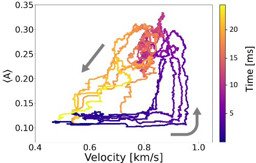
Figure 13: Trajectory of the ELM crash in the space spanned by average filament amplitude $\langle A\rangle\>$and poloidal velocity. Time relative to an ELM crash is encoded in color. Five trajectories are overlaid.

Figure 13 visualizes the strong correlation cycle between filament amplitude and poloidal velocity. Tracked over 5 ELM crash cycles, we observe a hysteresis curve where first the poloidal velocity increases while $\langle A\rangle\>$remains constant. In the following pre-crash phase, the filament amplitude increases while the poloidal velocity remains constant. The ELM crash phase is then characterized by a drop in filament amplitude from approximately $\langle A\rangle\>$$=0.3$ to $0.1$, and a simultaneous drop in filament velocity from approximately $1.0\mathrm{km/s}$ to $0.5\mathrm{km/s}$.

4 Discussion

The YOLO-based detector reliably identifies ELM filaments in normalized ECEI images. As a supervised algorithm, the detector requires manually labeled training data to be able to detect ELM filaments in images. The trained detector achieves $93.7\%$ accuracy on a validation set and manual inspection of predicted ELM filament bounding boxes shows a good performance across various stages of ELM phase. The size distribution of the manually labeled data is narrower than the distribution of bounding boxes detected during inference. A manual inspection of the identified bounding boxes suggests that the mismatching part of the distribution is characterized by lower IoU scores. But regardless, the predicted bounding boxes still reliably identify ELM filaments. This effect highlights the sensitivity of supervised machine learning models to the biases included in the training data. In general, one needs to take care of imbalance issues when developing data-driven methods and carefully compare the properties of the training data set and the data set identified during inference.

The trained detector is used to identify individual ELM filament crests for a $0.2\,\mathrm{s}$ long sub-interval of an ELM cycle. From the detection events, we calculate the average width and height, filament amplitude, as well as poloidal velocity. The bounding box dimensions of the detected filaments, as well as the count of detected filaments present quasi-periodic behavior that is strongly correlated with the spectrogram as well as $\langle A\rangle\>$. Identifying the change of the bounding box as the mode-number of the ELM, this behavior is indicative of non-linear interactions which modify the wavelength of the temperature perturbations. In particular, the width of the detected filaments changes from approximately $6\,\mathrm{cm}$ before ELM crashes to approximately $4\,\mathrm{cm}$ during the ELM crash. That is, by a factor of 1.5. At the same time, far fewer but hotter filaments are detected on average during the ELM crash.

A detailed analysis of $\langle A\rangle\>$in the periods leading up to an ELM crash shows a range of behaviors. Small growth phases can be followed by an intermediate saturation and reversals. This dithering between a ground state and a small elevated level appears random and no dynamics that are predictive of a following ELM crash are observed in the analyzed data.

Finally, we find a strong correlation between $\langle A\rangle\>$and the poloidal filament velocity. During each ELM crash, the average rotation velocity decreases by a factor of 2 from approximately $0.8\,\mathrm{km/s}$ to approximately $0.4\,\mathrm{km/s}$. After each ELM crash the poloidal velocity rapidly recovers to pre-crash levels. In the data shown here, there appears no characteristic time scale for any decrease or increase in poloidal rotation velocity. For example, the velocity decreases gradually in the first or 6th ELM crash shown in Fig. 12 while the velocity drop is more spontaneous for the 3rd and 4th crash. Finally, we show that the ELM cycle as observed in this single plasma follows a cyclical dynamic in the state space spanned by $\langle A\rangle\>$and the poloidal velocity.

The measurements of our machine-learning detector compare favorably with previous manual analyses, for example the reported ELM filament velocity range of 0.5 to 1.0 km/s agrees well with results presented for both, KSTAR [62, 63, 62, 61] and ASDEX upgrade[64, 63]. Both [65] and [66] report that ELM filament velocities decrease immediately before an ELM crash. Here, we verify this observation, and discover a hysteresis relation between the velocity and the amplitude. It has previously been suggested that radio frequency wave emission [67] might be responsible for this velocity reduction before the ELM crash and the hysteresis relation. Also, we found that the mode aspect ratio changes significantly just before the ELM crash, which is consistent with previous observations of solitary perturbation [61].

5 Summary and outlook

We use a machine learning model, based on the YOLO-v4 classifier, to detect ELM filaments in ECEI images. The developed detector performs robustly and is used to identify bounding boxes of ELM filaments during a $0.2\,\mathrm{s}$ long sub-interval. This data is used to investigate ELM filament dynamics. In particular, we compile filament dimensions, the average ELM filament amplitude, as well as the poloidal velocity of the filaments in the laboratory frame. For the analyzed ELM crashes, all these quantities present quasi-periodic behavior. Right after an ELM crash, the average filament amplitude is low, the average filament is about $4\,\mathrm{cm}$ wide and $6\,\mathrm{cm}$ tall and rotates counter-clockwise with about $0.8\,\mathrm{km/s}$. Leading up to an ELM crash, the average filament amplitude increases, and their width, as well as poloidal velocity, decreases. The average number of filaments visible per frame also decreases in the period leading up to an ELM crash. In other words, ELM crashes manifest as few, hot filaments. The quasi-periodic behavior can be interpreted as closed cycles in the phase space spanned by $\langle A\rangle\>$and the poloidal velocity.

Future work will focus on systematic investigations of ECEI data sampled during ELM cycles. The possibility to automatically collect variations in filament properties on a frame-by-frame basis may lead to further discovery. For example, this may aid in identifying solitary perturbations and distinguishing them from filamentary ELM structures, this allowing a more targeted investigation into the non-linear evolution of the underlying ELM instability physics. And finally, it may be desirable to condense the convolutional architecture of the used YOLO model into a simpler one, with still enough flexibility to identify ELM filaments in ECEI data.

6 Acknowledgements

This work was made possible by funding from the Department of Energy for the Summer Undergraduate Laboratory Internship (SULI) program. This work is supported by the US DOE Contract No. DE-AC02-09CH11466 and R&D Programs of ”KSTAR Experimental Collaboration and Fusion Plasma Research (EN2201-13)”. The authors report no conflicts of interest.

References

- [1] R. A. Moyer, K. H. Burrell, T. N. Carlstrom, S. Coda, R. W. Conn, E. J. Doyle, P. Gohil, R. J. Groebner, J. Kim, R. Lehmer, W. A. Peebles, M. Porkolab, C. L. Rettig, T. L. Rhodes, R. P. Seraydarian, R. Stockdale, D. M. Thomas, G. R. Tynan, and J. G. Watkins, “Beyond paradigm: Turbulence, transport, and the origin of the radial electric field in low to high confinement mode transitions in the DIII‐D tokamak,” Physics of Plasmas, 2, 6, 2397 (1995); 10.1063/1.871263., URL https://doi.org/10.1063/1.871263.
- [2] F. Wagner, “A quarter-century of H-mode studies,” Nuclear Fusion, 49, 12B, B1 (2007); 10.1088/0741-3335/49/12b/s01., URL https://doi.org/10.1088/0741-3335/49/12b/s01.
- [3] A. W. Leonard, “Edge-localized-modes in tokamaks,” Physics of Plasmas, 21, 9, 090501 (2014); 10.1063/1.4894742., URL https://doi.org/10.1063/1.4894742.
- [4] I. A. E. Agency, ITER Technical Basis, no. 24 in ITER EDA Documentation Series, INTERNATIONAL ATOMIC ENERGY AGENCY, Vienna (2002)URL https://www.iaea.org/publications/6492/iter-technical-basis.
- [5] S. Kim, T. Casper, and J. Snipes, “Investigation of key parameters for the development of reliable ITER baseline operation scenarios using CORSICA,” Nuclear Fusion, 58, 5, 056013 (2018); 10.1088/1741-4326/aab034., URL https://doi.org/10.1088/1741-4326/aab034.
- [6] D. Hill, “A review of ELMs in divertor tokamaks,” Journal of Nuclear Materials, 241-243, 182 (1997); https://doi.org/10.1016/S0022-3115(97)80039-6., URL https://www.sciencedirect.com/science/article/pii/S0022311597800396.
- [7] G. Lee, M. Kwon, C. Doh, B. Hong, K. Kim, M. Cho, W. Namkung, C. Chang, Y. Kim, J. Kim, H. Jhang, D. Lee, K. You, J. Han, M. Kyum, J. Choi, J. Hong, W. Kim, B. Kim, J. Choi, S. Seo, H. Na, H. Lee, S. Lee, S. Yoo, B. Lee, Y. Jung, J. Bak, H. Yang, S. Cho, K. Im, N. Hur, I. Yoo, J. Sa, K. Hong, G. Kim, B. Yoo, H. Ri, Y. Oh, Y. Kim, C. Choi, D. Kim, Y. Park, K. Cho, T. Ha, S. Hwang, Y. Kim, S. Baang, S. Lee, H. Chang, W. Choe, S. Jeong, S. Oh, H. Lee, B. Oh, B. Choi, C. Hwang, S. In, S. Jeong, I. Ko, Y. Bae, H. Kang, J. Kim, H. Ahn, D. Kim, C. Choi, J. Lee, Y. Lee, Y. Hwang, S. Hong, K.-H. Chung, D.-I. Choi, and K. Team, “Design and construction of the KSTAR tokamak,” Nuclear Fusion, 41, 10, 1515 (2001); 10.1088/0029-5515/41/10/318., URL https://doi.org/10.1088/0029-5515/41/10/318.
- [8] J.-W. Ahn, H.-S. Kim, Y. Park, L. Terzolo, W. Ko, J.-K. Park, A. England, S. Yoon, Y. Jeon, S. Sabbagh, Y. Bae, J. Bak, S. Hahn, D. Hillis, J. Kim, W. Kim, J. Kwak, K. Lee, Y. Na, Y. Nam, Y. Oh, and S. Park, “Confinement and ELM characteristics of H-mode plasmas in KSTAR,” Nuclear Fusion, 52, 11, 114001 (2012); 10.1088/0029-5515/52/11/114001., URL https://doi.org/10.1088/0029-5515/52/11/114001.
- [9] P. B. Snyder, H. R. Wilson, and X. Q. Xu, “Progress in the peeling-ballooning model of edge localized modes: Numerical studies of nonlinear dynamics,” Physics of Plasmas, 12, 5, 056115 (2005); 10.1063/1.1873792., URL https://doi.org/10.1063/1.1873792.
- [10] C. Ham, A. Kirk, S. Pamela, and H. Wilson, “Filamentary plasma eruptions and their control on the route to fusion energy,” Nature Reviews Physics, 2, 3, 159 (2020); 10.1038/s42254-019-0144-1., URL https://doi.org/10.1038/s42254-019-0144-1.
- [11] P. Snyder, R. Groebner, J. Hughes, T. Osborne, M. Beurskens, A. Leonard, H. Wilson, and X. Xu, “A first-principles predictive model of the pedestal height and width: development, testing and ITER optimization with the EPED model,” Nuclear Fusion, 51, 10, 103016 (2011); 10.1088/0029-5515/51/10/103016., URL https://doi.org/10.1088/0029-5515/51/10/103016.
- [12] Y. Oh, H. J. Hwang, M. Leconte, M. Kim, and G. S. Yun, “Effect of time-varying flow-shear on the nonlinear stability of the boundary of magnetized toroidal plasmas,” AIP Advances, 8, 2, 025224 (2018); 10.1063/1.5006554., URL https://doi.org/10.1063/1.5006554.
- [13] S. Kim, S. Pamela, O. Kwon, M. Becoulet, G. Huijsmans, Y. In, M. Hoelzl, J. Lee, M. Kim, G. Park, H. S. Kim, Y. Lee, G. Choi, C. Lee, A. Kirk, A. Thornton, and Y.-S. N. and, “Nonlinear modeling of the effect of n = 2 resonant magnetic field perturbation on peeling-ballooning modes in KSTAR,” Nuclear Fusion, 60, 2, 026009 (2020); 10.1088/1741-4326/ab5cf0., URL https://doi.org/10.1088/1741-4326/ab5cf0.
- [14] J. Kim, M. Choi, Y. Nam, H. Jhang, J. Bak, S. Hahn, C. Sung, W. Choe, and Y. c. Ghim, “Nonlinear energy transfer from low frequency electromagnetic fluctuations to broadband turbulence during edge localized mode crashes,” Nuclear Fusion, 60, 12, 124002 (2020); 10.1088/1741-4326/abb2d6., URL https://doi.org/10.1088/1741-4326/abb2d6.
- [15] G. S. Yun, W. Lee, M. J. Choi, J. B. Kim, H. K. Park, C. W. Domier, B. Tobias, T. Liang, X. Kong, N. C. Luhmann, and A. J. H. Donné, “Development of KSTAR ECE imaging system for measurement of temperature fluctuations and edge density fluctuations,” Review of Scientific Instruments, 81, 10, 10D930 (2010); 10.1063/1.3483209., URL https://doi.org/10.1063/1.3483209.
- [16] G. S. Yun, W. Lee, M. J. Choi, J. Lee, M. Kim, J. Leem, Y. Nam, G. H. Choe, H. K. Park, H. Park, D. S. Woo, K. W. Kim, C. W. Domier, N. C. Luhmann, N. Ito, A. Mase, and S. G. Lee, “Quasi 3D ECE imaging system for study of MHD instabilities in KSTAR,” Review of Scientific Instruments, 85, 11, 11D820 (2014); 10.1063/1.4890401., URL https://doi.org/10.1063/1.4890401.
- [17] G. S. Yun, W. Lee, M. J. Choi, J. Lee, H. K. Park, C. W. Domier, N. C. Luhmann, B. Tobias, A. J. H. Donné, J. H. Lee, Y. M. Jeon, and S. W. Yoon, “Two-dimensional imaging of edge-localized modes in KSTAR plasmas unperturbed and perturbed by n=1 external magnetic fields,” Physics of Plasmas, 19, 5, 056114 (2012); 10.1063/1.3694842., URL https://doi.org/10.1063/1.3694842.
- [18] H. K. Park, “Newly uncovered physics of MHD instabilities using 2-D electron cyclotron emission imaging system in toroidal plasmas,” Advances in Physics: X, 4, 1, 1633956 (2019); 10.1080/23746149.2019.1633956., URL https://doi.org/10.1080/23746149.2019.1633956.
- [19] J. A. Boedo, D. L. Rudakov, E. Hollmann, D. S. Gray, K. H. Burrell, R. A. Moyer, G. R. McKee, R. Fonck, P. C. Stangeby, T. E. Evans, P. B. Snyder, A. W. Leonard, M. A. Mahdavi, M. J. Schaffer, W. P. West, M. E. Fenstermacher, M. Groth, S. L. Allen, C. Lasnier, G. D. Porter, N. S. Wolf, R. J. Colchin, L. Zeng, G. Wang, J. G. Watkins, and T. Takahashi, “Edge-localized mode dynamics and transport in the scrape-off layer of the DIII-D tokamak,” Physics of Plasmas, 12, 7, 072516 (2005); 10.1063/1.1949224., URL https://doi.org/10.1063/1.1949224.
- [20] J. Terry, I. Cziegler, A. Hubbard, J. Snipes, J. Hughes, M. Greenwald, B. LaBombard, Y. Lin, P. Phillips, and S. Wukitch, “The dynamics and structure of edge-localized-modes in Alcator C-Mod,” Journal of Nuclear Materials, 363-365, 994 (2007); https://doi.org/10.1016/j.jnucmat.2007.01.266., URL https://www.sciencedirect.com/science/article/pii/S0022311507002048, plasma-Surface Interactions-17.
- [21] R. J. Maqueda and R. Maingi, “Primary edge localized mode filament structure in the National Spherical Torus Experiment,” Physics of Plasmas, 16, 5, 056117 (2009); 10.1063/1.3085798., URL https://doi.org/10.1063/1.3085798.
- [22] A. Diallo and F. M. Laggner, “Review: Turbulence dynamics during the pedestal evolution between edge localized modes in magnetic fusion devices,” Plasma Physics and Controlled Fusion, 63, 1, 013001 (2020); 10.1088/1361-6587/abbf85., URL https://doi.org/10.1088/1361-6587/abbf85, publisher: IOP Publishing.
- [23] J. Kates-Harbeck, A. Svyatkovskiy, and W. Tang, “Predicting disruptive instabilities in controlled fusion plasmas through deep learning,” Nature, 568, 7753, 526 (2019); 10.1038/s41586-019-1116-4., URL https://doi.org/10.1038/s41586-019-1116-4.
- [24] G. Sias, B. Cannas, S. Carcangiu, A. Fanni, A. Murari, A. Pau, and J. Contributors, “Disruption Prediction Approaches Using Machine Learning Tools in Tokamaks,” 2019 PhotonIcs Electromagnetics Research Symposium - Spring (PIERS-Spring), 2880–2890 (2019); 10.1109/PIERS-Spring46901.2019.9017280.
- [25] A. Pau, A. Fanni, S. Carcangiu, B. Cannas, G. Sias, A. Murari, and F. R. and, “A machine learning approach based on generative topographic mapping for disruption prevention and avoidance at JET,” Nuclear Fusion, 59, 10, 106017 (2019); 10.1088/1741-4326/ab2ea9., URL https://doi.org/10.1088/1741-4326/ab2ea9.
- [26] R. M. Churchill, B. Tobias, and Y. Zhu, “Deep convolutional neural networks for multi-scale time-series classification and application to tokamak disruption prediction using raw, high temporal resolution diagnostic data,” Physics of Plasmas, 27, 6, 062510 (2020); 10.1063/1.5144458., URL https://doi.org/10.1063/1.5144458.
- [27] Y. Fu, D. Eldon, K. Erickson, K. Kleijwegt, L. Lupin-Jimenez, M. D. Boyer, N. Eidietis, N. Barbour, O. Izacard, and E. Kolemen, “Machine learning control for disruption and tearing mode avoidance,” Physics of Plasmas, 27, 2, 022501 (2020); 10.1063/1.5125581., URL https://doi.org/10.1063/1.5125581.
- [28] B. H. Guo, B. Shen, D. L. Chen, C. Rea, R. S. Granetz, Y. Huang, L. Zeng, H. Zhang, J. P. Qian, Y. W. Sun, and B. J. Xiao, “Disruption prediction using a full convolutional neural network on EAST,” Plasma Physics and Controlled Fusion, 63, 2, 025008 (2020); 10.1088/1361-6587/abcbab., URL https://doi.org/10.1088/1361-6587/abcbab.
- [29] C. Rea, K. J. Montes, A. Pau, R. S. Granetz, and O. Sauter, “Progress Toward Interpretable Machine Learning–Based Disruption Predictors Across Tokamaks,” Fusion Science and Technology, 76, 8, 912 (2020); 10.1080/15361055.2020.1798589., URL https://doi.org/10.1080/15361055.2020.1798589.
- [30] M. Boyer, C. Rea, and M. Clement, “Toward active disruption avoidance via real-time estimation of the safe operating region and disruption proximity in tokamaks,” Nuclear Fusion, 62, 2, 026005 (2021); 10.1088/1741-4326/ac359e., URL https://doi.org/10.1088/1741-4326/ac359e.
- [31] J. Barr, B. Sammuli, D. Humphreys, E. Olofsson, X. Du, C. Rea, W. Wehner, M. Boyer, N. Eidietis, R. Granetz, A. Hyatt, T. Liu, N. Logan, S. Munaretto, E. Strait, Z. Wang, and the DIII-D Team, “Development and experimental qualification of novel disruption prevention techniques on DIII-D,” Nuclear Fusion, 61, 12, 126019 (2021); 10.1088/1741-4326/ac2d56., URL https://doi.org/10.1088/1741-4326/ac2d56.
- [32] W. Hu, C. Rea, Q. Yuan, K. Erickson, D. Chen, B. Shen, Y. Huang, J. Xiao, J. Chen, Y. Duan, Y. Zhang, H. Zhuang, J. Xu, K. Montes, R. Granetz, L. Zeng, J. Qian, B. Xiao, and J. Li, “Real-time prediction of high-density EAST disruptions using random forest,” Nuclear Fusion, 61, 6, 066034 (2021); 10.1088/1741-4326/abf74d., URL https://doi.org/10.1088/1741-4326/abf74d.
- [33] J. Degrave, F. Felici, J. Buchli, M. Neunert, B. Tracey, F. Carpanese, T. Ewalds, R. Hafner, A. Abdolmaleki, D. de las Casas, C. Donner, L. Fritz, C. Galperti, A. Huber, J. Keeling, M. Tsimpoukelli, J. Kay, A. Merle, J.-M. Moret, S. Noury, F. Pesamosca, D. Pfau, O. Sauter, C. Sommariva, S. Coda, B. Duval, A. Fasoli, P. Kohli, K. Kavukcuoglu, D. Hassabis, and M. Riedmiller, “Magnetic control of tokamak plasmas through deep reinforcement learning,” Nature, 602, 7897, 414 (2022); 10.1038/s41586-021-04301-9., URL https://doi.org/10.1038/s41586-021-04301-9.
- [34] E. Aymerich, G. Sias, F. Pisano, B. Cannas, S. Carcangiu, C. Sozzi, C. Stuart, P. Carvalho, and A. Fanni, “Disruption prediction at JET through Deep Convolutional Neural Networks using spatiotemporal information from plasma profiles,” Nuclear Fusion (2022)URL http://iopscience.iop.org/article/10.1088/1741-4326/ac525e.
- [35] S. Joung, J. Kim, S. Kwak, J. Bak, S. Lee, H. Han, H. Kim, G. Lee, D. Kwon, and Y.-C. Ghim, “Deep neural network Grad–Shafranov solver constrained with measured magnetic signals,” Nuclear Fusion, 60, 1, 016034 (2019); 10.1088/1741-4326/ab555f., URL https://doi.org/10.1088/1741-4326/ab555f.
- [36] K. L. van de Plassche, J. Citrin, C. Bourdelle, Y. Camenen, F. J. Casson, V. I. Dagnelie, F. Felici, A. Ho, and S. Van Mulders, “Fast modeling of turbulent transport in fusion plasmas using neural networks,” Physics of Plasmas, 27, 2, 022310 (2020); 10.1063/1.5134126., URL https://doi.org/10.1063/1.5134126.
- [37] A. Ho, J. Citrin, C. Bourdelle, Y. Camenen, F. J. Casson, K. L. van de Plassche, and H. Weisen, “Neural network surrogate of QuaLiKiz using JET experimental data to populate training space,” Physics of Plasmas, 28, 3, 032305 (2021); 10.1063/5.0038290., URL https://doi.org/10.1063/5.0038290.
- [38] A. A. Kaptanoglu, K. D. Morgan, C. J. Hansen, and S. L. Brunton, “Physics-constrained, low-dimensional models for magnetohydrodynamics: First-principles and data-driven approaches,” Phys. Rev. E, 104, 015206 (2021); 10.1103/PhysRevE.104.015206., URL https://link.aps.org/doi/10.1103/PhysRevE.104.015206.
- [39] H. LI, Y. FU, J. LI, and Z. WANG, “Machine learning of turbulent transport in fusion plasmas with neural network,” Plasma Science and Technology, 23, 11, 115102 (2021); 10.1088/2058-6272/ac15ec., URL https://doi.org/10.1088/2058-6272/ac15ec.
- [40] G. Dong, X. Wei, J. Bao, G. Brochard, Z. Lin, and W. Tang, “Deep learning based surrogate models for first-principles global simulations of fusion plasmas,” Nuclear Fusion, 61, 12, 126061 (2021); 10.1088/1741-4326/ac32f1., URL https://doi.org/10.1088/1741-4326/ac32f1.
- [41] A. Merlo, D. Böckenhoff, J. Schilling, U. Höfel, S. Kwak, J. Svensson, A. Pavone, S. A. Lazerson, and T. S. Pedersen, “Proof of concept of a fast surrogate model of the VMEC code via neural networks in Wendelstein 7-X scenarios,” Nuclear Fusion, 61, 9, 096039 (2021); 10.1088/1741-4326/ac1a0d., URL https://doi.org/10.1088/1741-4326/ac1a0d.
- [42] J. E. Lee, P. H. Seo, J. G. Bak, and G. S. Yun, “A machine learning approach to identify the universality of solitary perturbations accompanying boundary bursts in magnetized toroidal plasmas,” Scientific Reports, 11, 1, 3662 (2021); 10.1038/s41598-021-83192-2., URL https://doi.org/10.1038/s41598-021-83192-2.
- [43] S. J. Zweben, D. P. Stotler, J. L. Terry, B. LaBombard, M. Greenwald, M. Muterspaugh, C. S. Pitcher, K. Hallatschek, R. J. Maqueda, B. Rogers, J. L. Lowrance, V. J. Mastrocola, and G. F. Renda, “Edge turbulence imaging in the Alcator C-Mod tokamak,” Physics of Plasmas, 9, 5, 1981 (2002); 10.1063/1.1445179., URL http://dx.doi.org/10.1063/1.1445179.
- [44] R. Kube, O. Garcia, B. LaBombard, J. Terry, and S. Zweben, “Blob sizes and velocities in the Alcator C-Mod scrape-off layer,” Journal of Nuclear Materials, 438, S505 (2013); https://doi.org/10.1016/j.jnucmat.2013.01.104., URL https://www.sciencedirect.com/science/article/pii/S0022311513001128, proceedings of the 20th International Conference on Plasma-Surface Interactions in Controlled Fusion Devices.
- [45] S. Zweben, W. Davis, S. Kaye, J. Myra, R. Bell, B. LeBlanc, R. Maqueda, T. Munsat, S. Sabbagh, Y. Sechrest, and D. S. and, “Edge and SOL turbulence and blob variations over a large database in NSTX,” Nuclear Fusion, 55, 9, 093035 (2015); 10.1088/0029-5515/55/9/093035., URL https://doi.org/10.1088/0029-5515/55/9/093035.
- [46] G. Decristoforo, F. Militello, T. Nicholas, J. Omotani, C. Marsden, N. Walkden, and O. E. Garcia, “Blob interactions in 2D scrape-off layer simulations,” Physics of Plasmas, 27, 12, 122301 (2020); 10.1063/5.0021314., URL https://doi.org/10.1063/5.0021314.
- [47] M. Agostini, J. Terry, P. Scarin, and S. Zweben, “Edge turbulence in different density regimes in Alcator C-Mod experiment,” Nuclear Fusion, 51, 5, 053020 (2011); 10.1088/0029-5515/51/5/053020., URL https://doi.org/10.1088/0029-5515/51/5/053020.
- [48] M. Lampert, A. Diallo, and S. J. Zweben, “Novel 2D velocity estimation method for large transient events in plasmas,” Review of Scientific Instruments, 92, 8, 083508 (2021); 10.1063/5.0058216., URL https://doi.org/10.1063/5.0058216.
- [49] M. Imre, J. Han, J. Dominski, M. Churchill, R. Kube, C.-S. Chang, T. Peterka, H. Guo, and C. Wang, “ContourNet: Salient Local Contour Identification for Blob Detection in Plasma Fusion Simulation Data,” G. Bebis, R. Boyle, B. Parvin, D. Koracin, D. Ushizima, S. Chai, S. Sueda, X. Lin, A. Lu, D. Thalmann, C. Wang, and P. Xu (Editors), Advances in Visual Computing, 289–301, Springer International Publishing, Cham (2019).
- [50] I. H. Hutchinson, Principles of Plasma Diagnostics, Cambridge University Press (2002); 10.1017/CBO9780511613630.
- [51] J. Redmon, S. K. Divvala, R. B. Girshick, and A. Farhadi, “You Only Look Once: Unified, Real-Time Object Detection,” CoRR, abs/1506.02640 (2015)URL http://arxiv.org/abs/1506.02640.
- [52] A. Bochkovskiy, C.-Y. Wang, and H.-Y. M. Liao, “YOLOv4: Optimal Speed and Accuracy of Object Detection,” (2020).
- [53] C. Wang, A. Bochkovskiy, and H. M. Liao, “Scaled-YOLOv4: Scaling Cross Stage Partial Network,” CoRR, abs/2011.08036 (2020)URL https://arxiv.org/abs/2011.08036.
- [54] L. Jiao, F. Zhang, F. Liu, S. Yang, L. Li, Z. Feng, and R. Qu, “A Survey of Deep Learning-based Object Detection,” CoRR, abs/1907.09408 (2019)URL http://arxiv.org/abs/1907.09408.
- [55] S. Ren, K. He, R. Girshick, X. Zhang, and J. Sun, “Object Detection Networks on Convolutional Feature Maps,” IEEE Transactions on Pattern Analysis and Machine Intelligence, 39, 7, 1476 (2017); 10.1109/TPAMI.2016.2601099.
- [56] S. Chakraborty, S. Paul, R. Sarkar, and M. Nasipuri, “Feature Map Reduction in CNN for Handwritten Digit Recognition,” J. Kalita, V. E. Balas, S. Borah, and R. Pradhan (Editors), Recent Developments in Machine Learning and Data Analytics, 143–148, Springer Singapore, Singapore (2019).
- [57] L. Alzubaidi, J. Zhang, A. J. Humaidi, A. Al-Dujaili, Y. Duan, O. Al-Shamma, J. Santamaría, M. A. Fadhel, M. Al-Amidie, and L. Farhan, “Review of deep learning: concepts, CNN architectures, challenges, applications, future directions,” J Big Data, 8, 53 (2021)URL https://doi.org/10.1186/s40537-021-00444-8.
- [58] D. P. Kingma and J. Ba, “Adam: A Method for Stochastic Optimization,” (2014); 10.48550/ARXIV.1412.6980., URL https://arxiv.org/abs/1412.6980.
- [59] L. Lao, H. S. John, R. Stambaugh, and W. Pfeiffer, “Separation of beta-p and l-i in tokamaks of non-circular cross-section,” Nuclear Fusion, 25, 10, 1421 (1985); 10.1088/0029-5515/25/10/004., URL https://doi.org/10.1088/0029-5515/25/10/004.
- [60] O. Meneghini, S. Smith, L. Lao, O. Izacard, Q. Ren, J. Park, J. Candy, Z. Wang, C. Luna, V. Izzo, B. Grierson, P. Snyder, C. Holland, J. Penna, G. Lu, P. Raum, A. McCubbin, D. Orlov, E. Belli, N. Ferraro, R. Prater, T. Osborne, A. Turnbull, and G. Staebler, “Integrated modeling applications for tokamak experiments with OMFIT,” Nuclear Fusion, 55, 8, 083008 (2015)URL http://iopscience.iop.org/article/10.1088/0029-5515/55/8/083008/meta.
- [61] J. E. Lee, G. S. Yun, W. Lee, M. H. Kim, M. Choi, J. Lee, M. Kim, H. K. Park, J. G. Bak, W. H. Ko, and Y. S. Park, “Solitary perturbations in the steep boundary of magnetized toroidal plasma,” Scientific Reports, 7, 1, 45075 (2017); 10.1038/srep45075., URL https://doi.org/10.1038/srep45075.
- [62] M. J. Choi, G. S. Yun, and W. Lee, “Detailed 2-D imaging of growth and burst of edge-localized filaments in KSTAR H-mode plasmas Network.” Presented at 38th EPS Conference on Plasma Physics. (2011).
- [63] B. Vanovac, E. Wolfrum, M. Hoelzl, M. Willensdorfer, M. Cavedon, G. Harrer, F. Mink, S. Denk, S. Freethy, M. Dunne, P. Manz, and N. L. and, “Characterization of low-frequency inter-ELM modes of H-mode discharges at ASDEX Upgrade,” Nuclear Fusion, 58, 11, 112011 (2018); 10.1088/1741-4326/aada20., URL https://doi.org/10.1088/1741-4326/aada20.
- [64] J. Boom, I. Classen, P. de Vries, T. Eich, E. Wolfrum, W. Suttrop, R. Wenninger, A. Donné, B. Tobias, C. Domier, N. Luhmann, and H. P. and, “2D ECE measurements of type-I edge localized modes at ASDEX Upgrade,” Nuclear Fusion, 51, 10, 103039 (2011); 10.1088/0029-5515/51/10/103039., URL https://doi.org/10.1088/0029-5515/51/10/103039.
- [65] G. S. Yun, W. Lee, M. J. Choi, J. Lee, H. K. Park, B. Tobias, C. W. Domier, N. C. Luhmann, A. J. H. Donné, and J. H. Lee, “Two-Dimensional Visualization of Growth and Burst of the Edge-Localized Filaments in KSTAR -Mode Plasmas,” Phys. Rev. Lett., 107, 045004 (2011); 10.1103/PhysRevLett.107.045004., URL https://link.aps.org/doi/10.1103/PhysRevLett.107.045004.
- [66] A. Bogomolov, I. Classen, J. Boom, A. Donné, E. Wolfrum, R. Fischer, E. Viezzer, P. Schneider, P. Manz, W. Suttrop, and N. Luhmann, “Study of the ELM fluctuation characteristics during the mitigation of type-I ELMs,” Nuclear Fusion, 55, 8, 083018 (2015); 10.1088/0029-5515/55/8/083018., URL https://doi.org/10.1088/0029-5515/55/8/083018.
- [67] M. Kim, S. Thatipamula, J. Kim, M. Choi, J. Lee, W. Lee, M. Kim, Y. Yoon, and G. Yun, “Intense whistler-frequency emissions at the pedestal collapse in KSTAR H-mode plasmas,” Nuclear Fusion, 60, 12, 126021 (2020); 10.1088/1741-4326/abb25c., URL https://doi.org/10.1088/1741-4326/abb25c.