Complexity from Adaptive-Symmetries Breaking:
Global Minima in the Statistical Mechanics of Deep Neural Networks

Abstract

Background

The scientific understanding of complex systems and deep neural networks (DNNs) are among the unsolved important problems of science; and DNNs are evidently complex systems. Meanwhile, conservative symmetry arguably is the most important concept of physics, and P.W. Anderson, Nobel Laureate in physics, speculated that increasingly sophisticated broken symmetry in many-body systems correlates with increasing complexity and functional specialization. Furthermore, in complex systems such as DNA molecules, different nucleotide sequences consist of different weak bonds with similar free energy; and energy fluctuations would break the symmetries that conserve the free energy of the nucleotide sequences, which selected by the environment would lead to organisms with different phenotypes.

Purpose

When the molecule is very large, we might speculate that statistically the system poses in a state that would be of equal probability to transit to a large number of adjacent possible states; that is, an adaptive symmetry whose breaking is selected by the feedback signals from the environment. In physics, quantitative changes would accumulate into qualitative revolution where previous paradoxical behaviors are reconciled under a new paradigm of higher dimensionality (e.g., wave-particle duality in quantum physics). This emergence of adaptive symmetry and complexity might be speculated as accumulation of sophistication and quantity of conservative symmetries that lead to a paradigm shift, which might clarify the behaviors of DNNs.

Results

In this work, theoretically and experimentally, we characterize the optimization process of a DNN system as an extended symmetry-breaking process where novel examples are informational perturbations to the system that breaks adaptive symmetries. One particular finding is that a hierarchically large DNN would have a large reservoir of adaptive symmetries, and when the information capacity of the reservoir exceeds the complexity of the dataset, the system could absorb all perturbations of the examples and self-organize into a functional structure of zero training errors measured by a certain surrogate risk. In this diachronically extended process, complexity emerges from quantitative accumulation of adaptive-symmetries breaking.

Method

More specifically, this process is characterized by a statistical-mechanical model that could be appreciated as a generalization of statistics physics to the DNN organized complex system, and characterizes regularities in higher dimensionality. The model consists of three constitutes that could be appreciated as the counterparts of Boltzmann distribution, Ising model, and conservative symmetry, respectively: (1) a stochastic definition/interpretation of DNNs that is a multilayer probabilistic graphical model, (2) a formalism of circuits that perform biological computation, (3) a circuit symmetry from which self-similarity between the microscopic and the macroscopic adaptability manifests. The model is analyzed with a method referred as the statistical assembly method that analyzes the coarse-grained behaviors (over a symmetry group) of the heterogeneous hierarchical many-body interaction in DNNs.

Conclusion

Overall, this characterization suggests a physical-biological-complex scientific understanding to the optimization power of DNNs.

I Introduction

In formulating the concept of organized complex systems [1, 2, 3, 4, 5, 6, 7], P. Anderson, described in the seminal essay More is Different that, “it is only slightly overstating the case to say that physics is the study of symmetry” [3, p. 393], and in the same essay, he prefigured [3, p. 396]: “… at some point we harre to stop talking about decreasing symmetry and start calling it increasing complication …” in “… functional structure in a teleological sense …”—teleology refers to goal-directed behaviors controlled by feedback [8], and in modern terminology, complication is referred as complexity. Organized complex systems are adaptive systems emerge from a large number of locally nonlinearly interacting units and cannot be reduced to a linear superposition of the constituent units. Despite the progress, the study of organized complex systems (e.g., biotic, neural, economical, and social systems) is still a long way from developing into a science as solid as physics [9]. And the field has been considered to be in a state of “waiting for Carnot”; that is, the field is waiting for the right concepts and mathematics to be formulated to describe the many forms of complexity in nature [4, p. 302].

This tension between seemingly incomprehensible complexity and inquiry of science also underlies the field of Deep Neural Networks (DNNs) [10]. DNNs have solved marvelous engineering problems [11, 12, 13], and posit to contribute to societal challenges [14] and difficult scientific problems [15], but could also induce disruptive societal changes [16, 17]. However, the theoretical understanding of DNNs is rather limited [18] for the same reason of that of complex systems: a DNN is an organized complex system hierarchically composed by an indefinite number of elementary nonlinear modules. The limit in understanding manifests in the optimization properties [19, 20, 21] and generalization ability [11, 22, 23], and results in critical weakness such as interpretability [24, 25], uncertainty quantification [26, 27], and adversarial robustness [28, 29], harbingering the next wave of Artificial Intelligence [30].

This situation is not unsimilar to the state of physics at the turn of the 20th century [31, 32]. In the edifice of Classic Physics, a few seemingly incomprehensible phenomena questioned the fundamental assumptions of contemporary physics (i.e., black-body radiation and photoelectric effect), and catalyzed the development of Quantum Physics. When a field of science sufficiently mature in the sense of explaining all existing phenomena, the reconciliation of paradoxical properties of a system in the existing science with a new “science” is summarized by Thomas S. Kuhn [33] as paradigm shift (e.g. wave-particle duality in quantum physics, and the mass-energy equivalence in special relativity). And a commonality of the paradigm shifts is that quantitative change accumulates into qualitative revolution, and the previous paradoxical behaviors are resolved by a model of higher dimensionality: the phenomena reduced to quantum scale need quantum physics, and are characterized not by point mass as a particle or a basis function (which is an infinitely long vector) of a particular frequency as a wave, but the probability of being in certain states that are eigenvectors of a matrix; and the phenomena at the speed of light need the special theory of relativity, and are characterized by a spatial-temporal four dimensional model that incorporates the speed of light, instead of the spatial three dimensional model.

In this work, we develop a characterization of the optimization process of DNNs’ that could be appreciated under this concept of paradigm shift; that is, a DNN being a statistical-mechanical system, as the sophistication and quantity of symmetries increases quantitatively, the statistical mechanics of this DNN organized complex system needs to and could be characterized by concepts of higher dimensionality than the ones in the statistical physics of disorganized complex systems. This characterization suggests a scientific—in the sense of epistemology and methodology of physics [1, 34, 35, 36, 37, 38], and of the philosophy of falsifiable science [39]—understanding of the optimization process and thus the optimization power of DNNs; a particular interesting result is that, informally stated, global minima of DNNs could be reached when the potential complexity of the DNN (which could be enlarged by making the DNN hierarchically large) is larger than the complexity of the dataset.

The formal characterization of this process would require us to visit the epistemological foundation of physics [34, 40, 1, 35, 36, 37, 38], to extend biologists and complexity scientists’ revision of this foundation [41, 1, 42, 43, 44, 45, 46, 36, 37, 38, 47, 48, 49, 50, 51, 52], and to leverage on recent progress in probability and statistics [53, 54, 55, 56]. Furthermore, we need to come up a statistical-mechanical model of the DNN organized complex system consisting of three constituents that could be appreciated as the counterparts of Boltzmann distribution, Ising model, conservative symmetry, respectively of statistical-physical models. The resulted model is analyzed with a method referred as the statistical assembly method that analyzes the coarse-grained behaviors (over a symmetry group) of the heterogeneous hierarchical many-body interaction in DNNs.

Therefore, to increase readability, this work is presented in a fractal style: we have written a short letter [57] to give a high level overview of the results, and it is advised to read the letter first; in this article, we shall elaborate the overview there. To begin with, we shortly summarize the main messages in the letter [57] in the next paragraphs.

By discussing the epistemology of physics, where the renormalizibility of physical systems [58, 59, 60] is an emergent organizing principle founding on conservative symmetries [3, 61] in which the microscopic details are unknowable or irrelevant [34], we motivate that we might need to investigate mesoscopic organizing principles of organized complex systems [40] that are stable [62] from an informational perspective [46, 49, 63, 64, 51]. The proliferation of adjacent states [7, p. 263] with similar free energy (i.e., conservative symmetric states) in DNA macromolecules [50], and the transitions among those states by the breaking conservative symmetries (induced by spontaneous symmetry breaking in quantum field theories or deterministic chaos [65, 61]) make us speculate that the lack of conservative symmetries in DNNs [66, 67] is a feature looked in a backward perspective.

The symmetry breaking in biology [45, 37, 68] breaks the symmetry of adaptation: the system has the capacity to process the novel information—that is, to adapt—by posing in states where symmetric possible directions to adapt could be adopted, which is in turn induced by the complex cooperative interaction among the heterogeneous units in a biotic system; and the symmetric states would break in response to random fluctuations and external feedback signals [45]. Thus, increased sophistication and quantity of conservative symmetries might lead to an antithetical concept of adaptive symmetry: unlike the symmetries in physics, which formalizes a conservative law that conserves the free energy of different states related by certain transformations and thus characterizes the invariant of free energy, the adaptive symmetry is the conservation of change of free energy; or in other words, the invariant of change that emerges as a result of the increased sophistication and quantity of conservative symmetries. Furthermore, in a complex adaptive system, a microscopic change at one scale has implications that ramify across scales throughout the system [69, 70], and thus regularities are not to be found in coarse-grained static behaviors where higher-order coupling is considered irrelevant fluctuations, but in the dynamic behaviors of adaptation [37, 47, 48, 52].

Motivated by the speculation, we investigate and find self-similar phenomena in DNNs where the output of a DNN (macroscopic behaviors) is the coarse-graining of basis units composed by neurons (that are referred as basis circuits, and are microscopic behaviors), and both the DNN and the basis circuits are dynamical feedback-control loops [8, 41, 71] (between the system and the environment) that are of adaptive symmetry. This self-similarity is concentration-of-measure phenomena that are of higher intrinsic dimensionality than those of disorganized complex physical systems. And complex functional structure emerges in a diachronic process of adaptive-symmetries breaking in response to feedback signals. Furthermore, during the process, intact and broken adaptive symmetries coexist—the former maintains the adaptability of the system, and the latter manifests as functional structure. Thus, for a hierarchically large enough DNN (relative to the dataset), a phenomenon exists such that sufficient adaptive-symmetries enable convergence to global minima in DNN optimization, and this process is an extended symmetries-breaking process that is both a phase and a phase transition—ringing a bell of paradigm shift.

In this article, we elaborate the results discussed only briefly in the letter [57]. In the rest of the introduction, we shall give the outline. And in the main body we shall mostly discuss the theoretical results conceptually at an intuitive level of formalism along with experimental results. We also have a formal presentation from an axiomatic approach in the sense of Hilbert’s sixth problem [72]; but the rigor and heavy math in this style are likely only interesting to a small subset of the audience, and thus the formal version of the main results is given in the supplementary material [73].

I.1 Outline

I.1.1 Statistical-mechanical model of DNN complex system

The constitutes of the statistical-mechanical model of DNNs is introduced from section II.1 to II.4. The constituents are introduced succinctly as follows.

1. First, in section II.1, we introduce a system that does statistical inference on hierarchical events, which is contextualized as a measure-theoretical formalism of the concept Umwelt in theoretical biology. More specifically, a statistical characterization (i.e., Boltzmann distribution) of the behaviors of disorganized complex systems is possible because despite the unpredictable behaviors of individual units, these irregularities are subdued into predictable aggregate behaviors of a vast number of units that are subject to average-energy constraints. Complex biotic systems also have such mixture of irregularities and predictability: evolution of biotic systems are both the result, of random events at all levels of organization of life and, of the constraint of possible evolutionary paths—the paths are selected by interaction with the ecosystem and the maintenance of a possibly renewed internal coherent structure of the organism that are constructed through its history [38]. The proposed Umwelt is a statistical-inference system that models this phenomenon under the context of DNNs. Compared with the disorganized complexity in statistical physical, where a system maximizes entropy subject to the constraint that system’s energy (i.e., the average of energy of units) is of a certain value, an Umwelt organized-complex system maximizes entropy subject to hierarchical event coupling such that it estimates the probability measures of groups of events in the environment that forms a hierarchy, and the probability measure of certain coarse-grained events with fitness consequences are estimated and could be used to predict future events.

2. Second, in section II.2, we introduce a stochastic definition of DNNs, that is an implementation of the Umwelt—through a hierarchical parameterization scheme that estimates probability measures (for the statistical inference problem of Umwelt) by dynamical programming, and an approximation inference method—and is a supervised DNN with the ReLU activation function. The definition defines a DNN as a multilayer probabilistic graphical model that is a hybrid of Markov random field and Bayesian network. The definition could be appreciated as a sophisticated deep higher-order Boltzmann machine with priors on weights, though there are critical differences, which is discussed in supp. A A with related works for interested readers.

3. Third, in section II.3, motivated by biological circuits, we introduce a formalism of circuits upon the stochastic definition of DNNs that formalizes the risk minimization of a DNN as a self-organizing informational-physical process where the system self-organizes to minimize a potential function referred as variational free energy that approximates the entropy of the environment by executing a feedback-control loop. The loop is composed by the hierarchical basis circuits (implemented by coupling among neurons) and a coarse-grained random variable (of fitness consequences) computed by the circuits. And each basis circuit is a microscopic feedback-control loop, and the coarse-grained effect of all the microscopic loops computes the coarse-grained variable. Under this circuit formalism, a basis circuit is like a spin in the Ising model; for example, the order parameter of DNNs derived from the circuit formalism is symbolically (but only symbolically) equivalent to the spin glass order parameter—order parameter of DNNs is introduced in section II.5.

4. Fourth, in section II.4, we introduce an adaptive symmetry, referred as circuit symmetry, of the basis circuits that characterize the phenomenon that each basis circuit is of a symmetric probability distribution, and thus of equal probability to contribute to the coarse-grained variable positively or negatively. The symmetry could break to a positive or negative value in response to feedback signals, and thus reduces risk. The symmetry is a heterogeneous symmetry (which shall be further explained in section II.4), implying that intact and broken circuit symmetries could coexist in a DNNs: the broken circuit symmetries encodes information about the environment (i.e., datasets), and the intact circuit symmetries maintain the adaptability to further reduce informational perturbations (i.e., training examples with nonzero risk). Adaptive symmetries are not symmetries typically in physics that conserve systems’ free energy (which is referred as conservative symmetries in this work). This epistemological difference is introduced in section II.4.1. To analyze the adaptive symmetries, a synthesis of statistical field theory and statistical learning theory is developed, and is referred as statistical assembly methods. The method analyzes the coarse-grained behaviors of basis circuits summed over symmetries group that turn out to be self-similar to the behaviors of basis circuits—which is similar to what the renormalization group technique reveals for the coarse-grained effect of symmetries in physics.

I.1.2 Extended symmetry breaking of DNNs

The symmetry breaking process of DNNs is introduced from in section II.5 and II.6. We also lightly discuss the paradox under the context of complexity science that the adaptive-symmetries breaking processing is both a phase and a phase transition in section III. The key messages of the sections are summarized as follows.

1. In section II.5, we introduce the order of DNNs, which generalizes the order in statistical physics (e.g., the magnetization is the order of a magnet) and the order in self-organization (i.e., order from noise/fluctuations/chaos), and characterizes the coarse-grained effect of circuit symmetries in a DNN to continue absorbing informational perturbations; that is, the capability of a DNN to decrease risk.

2. In section II.6, we introduce a phase of DNNs, which is referred as the plasticity phase. In this phase, while a DNN continually breaks circuit symmetries to reduce informational perturbations, the large reservoir of circuit symmetries result in that circuit symmetries stably exist (along with broken circuit symmetries), and the system manifests a self-similarity between the basis circuit (i.e., microscopic feedback-control loop) and the macroscopic/coarse-grained adaptive symmetry at the level of neuron assemblies (i.e., macroscopic/coarse-grained feedback-control loop). Both the gradient and Hessian are computed by neuron assemblies, and thus are of the adaptive symmetry; more specifically, the both the gradient, and eigenspectrum of Hessian are of a symmetric distribution—a subtlety exists in the problem setting of this work, and strictly speaking it is not that the eigenspectrum of Hessian is symmetric but a matrix in a decomposed form of Hessian. The phase is both a phase of a DNN, where the DNN could continually decreases risk, and an extended symmetry-breaking process, where the symmetries are continually being broken during the self-organizing process. As a result, all stationary points are saddle points, and benign pathways on the risk landscape of DNNs to zero risk could be found by following gradients. Overall, the results suggest an explanation of the optimization power of DNNs.

The training of a DNN is both an extended symmetry-breaking process, and a plasticity phase with stable symmetries. This superficially looks like a paradox: in physics, symmetry breaking is usually a singular phase transition. However, the unification of previously paradoxical properties of a system/object has repeatedly happened in the history of physics: at the quantum scale, wave and particle become a duality in quantum physics, and at the speed of light, the mass and energy become equivalent in special relativity. This is referred as the paradigm shift by Thomas S. Kuhn [33]. Thus, section III aims to address possible confusions by outlining a very crude look at the whole of the symmetry-breaking process of DNNs, and relating this work to complexity science [2, 3, 4, 5, 6, 7].

Discussion.

More particularly, the increased sophistication and quantity of symmetries of biotic systems makes symmetry-breaking gradually transits from a singular process to a continual process, and the plasticity phase could be understood as a diachronic process of evolving: when upper limit/bound of the complexity of the system is larger than the complexity of the environment where the system embodies, the system could perfectly approximate the organization/entropy of the environment (measured in surrogate risk). And the self-organizing process of DNNs is summarized as complexity from adaptive-symmetries breaking, which characterizes a process where a system computes to encoded increasing complex information by breaking adaptive symmetries.

I.1.3 Problem setting

Theoretical setting.

To conclude the introduction, we summarize the setting of the theoretical characterization in section II.7. Einstein said in a lecture in 1933, “it can scarcely be denied that the supreme goal of all theory is to make the irreducible basic elements as simple and as few as possible without having to surrender the adequate representation of a single datum of experience”[74]. We identify such a minimal irreducible DNN system that roughly is a hierarchically large deep/multilayer neural networks with ReLU activation function and a feedforward architecture, doing binary classification on real-world data whose complexity is less than the potential complexity of the network. As a clarifying note, we have mentioned in section I.1.2 in the passing that a subtlety exists in the symmetry of Hessian’s eigenspectrum. The subtlety comes from the class of loss functions that this paper works with, which is introduced in section II.7.

Experimental setting.

We also validate theoretical characterizations with experiments as the narrative develops. In the experiments, we train a VGGNet [75] (cross entropy loss replaced by the hinge loss) on the CIFAR10 datasets modified for binary classification. The DNN has $12$ layer, $\sim 10^{7}$ parameters/weights. More details of the experiment setting is given in supp. H B. The experiments should be understood as simulations that validate the theoretical characterizations. And to appreciate the simulation, existing works that does finite-size correction through statistical field theory to the works that study DNNs in the infinite-width setting tend to validate theoretical characterizations by running on toy models processing toy, or unrealistic datasets; for example, Cohen et al. [76] test the theory with four-layer large-width MLP on data uniformly sampled from a hypersphere, and justify their simplification by stating that expecting analytical characterization of networks of VGG architecture on ImageNet would be to expect “an analytical computation based on thermodynamics to capture the efficiency of a modern car engine or one based on Naiver-Stoke’s equations to output a better shape of a wing [76, p. 11]”; further contexts on existing works motivated by statistical field theory could be found in supp. A D. Though we only run simulation with a VGG network on a classic small dataset CIFAR10, this should be considered as a supportive experimental validation of the theoretical characterizations, and a start towards industrial settings, considering the difficulty of the problem.

I.1.4 Related works

The narrative of this work resolves around the characterization that the optimization of DNNs is an extended symmetry-breaking, and ends at an explanation of the optimization power of DNNs. Meanwhile, the narrative is composed by a stochastic definition/model of DNNs, a circuit formalism that analyzes the model, an epistemologically different symmetry (i.e., adaptive symmetry) with the conservative symmetry of physics, and the study of order and a phase of DNNs through the so call statistical assembly methods. Each of these components have extensive related works on its own, except for the circuit formalism, which should be appreciated as a technique that analyzes and accompanies the statistical definition. Therefore, to put the resultts under more specialized context, in addition to the background discussed extensively in the main body, we also collect discussion on these related works separately in supp. A for interested readers.

More specifically, first, the stochastic definition of DNNs in this work is a stochastic DNN, and also a Bayesian DNN, and thus existing works that study stochastic neural networks and Bayesian neural networks are discussed in supp. A A. Second, existing works that interpret the operation of DNNs as circuits are discussed in supp. A B, which is very short because they are only remotely related. Third, existing works that study symmetries of DNNs are discussed in supp. A C. Fourth, related works that study the optimization and phases of DNNs are discussed in supp. A D, by putting this works under the context of related works that study the risk landscape under the overparameterized regimen, and the phases of DNNs.

I.2 Notations

Normal letters denote scalar (e.g., $f$); bold, lowercase letters denote vectors (e.g., $\bm{x}$); bold, uppercase letters denote matrices, or random matrices (e.g., $\bm{W}$); normal, uppercase letters denote random elements/variables (e.g., $H$). $\text{dg}(\bm{h})$ denotes a diagonal matrix whose the diagonal is the vector $\bm{h}$. $:=$ denotes the “define” symbol: $x:=y$ defines a new symbol $x$ by equating it with $y$. A sequence of positive integer is also conveniently denoted as $[N]:=\{1,\ldots,N\}$. $\mathbb{B}$ denotes $\{0,1\}$. The upper arrow on operations denotes the direction: for example, $\overrightarrow{\Pi}_{i=1}^{n}\bm{W}_{i},\overleftarrow{\Pi}_{i=1}^{n}\bm{W}_{i},i<n,i,n\in\mathbb{N}$ denote $\bm{W}_{1}\ldots\bm{W}_{n},\bm{W}_{n}\ldots\bm{W}_{1}$, respectively. $\bm{i}_{p:q}$ denotes the subvector of $\bm{i}$ that is sliced from the $p^{th}$ component to $q^{th}$ (exclusive; that is, $i_{q}$ is excluded). This is the conventional in most programming languages to slice arrays. If the ending index is omitted, e.g., $\bm{i}_{p:}$, it denotes the subvector sliced from the $p^{th}$ component until the end (inclusive); similarly, if the starting index is omitted, e.g., $\bm{i}_{:q}$, it denotes the subvector sliced from the beginning (inclusive) until the $q^{th}$ component (exclusive). Because we shall deal with random variables in a multilayer network, we need the indices to denote the layers. When the lower index is not occupied, we use the lower index to denote a layer; for example, random vector at layer $l$ is denoted $H_{l}$. Otherwise, we put the layer index onto the upper index; for example $H^{l}_{i}$ denotes $i^{th}$ component of $H_{l}$. If matrices are indexed, we move the index up when indexing its entries, i.e., $w^{1}_{ij}$ denotes the $ij$th entry of $\bm{W}_{1}$. The other notations should be self-evident.

II Main results

II.1 Umwelt: system that does statistical inference on hierarchical events

II.1.1 Boltzmann distribution, disorganized complexity, complex biotic systems and DNNs

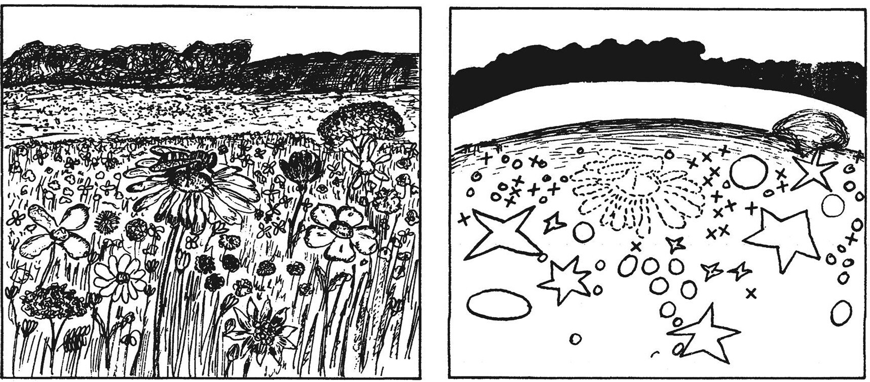
Figure 1: Environment and Umwelt of a honey bee, illstration from Uexküll [77, p. 351]. On the left is the environment observed by an external observer. On the right is the Umwelt of honey bees, which consists of the events (observations of certain objects) that have effects on the honey bees (e.g., the flowers with nectar), and bees could have an effect on (e.g., gathering the nectar). In this work, we formalize the emergence of an Umwelt as a statistical-inference process that estimates the probability measures of groups of events in the environment that forms a hierarchy, such that the probability measure of certain coarse-grained events with fitness consequences (e.g., detection of flowers with nectar) are estimated and could be used to predict future events. The probability measures are estimated through hierarchical entropy maximization subject to constraints that characterize hierarchical event coupling. With a hierarchical parameterization scheme that estimates probability measures through dynamical programming, and a particular choice of approximated inference method, the probability-estimation/learning algorithm of Umwelt is an expectation-maximization algorithm that corresponds to the forward-backward supervised training of a DNN with ReLU activation function. This formalism leads to a stochastic (whitebox) definition of DNNs that is a multilayer probabilistic graphical model.

In the 19th century, Ludwig Boltzmann provided a statistical mechanic model of gases at thermal equilibrium that provided a causal characterization of macroscopic thermodynamic behaviors of gases from microscopic gas molecules. The model characterizes a phenomenon that could be informally stated as: the gas in a container consists of billions of atoms that would predominantly stay close to certain states dictated by the system’s energy, and their chance of being in other states decreases exponentially; the probability distribution in the model is known as the Boltzmann distribution. Despite the exactness and clarity now conveyed by the model, the model was proposed among deep philosophical confusions, which could be summarized by the great debate between Ernst Mach and L. Boltzmann: “Boltzmann needed atoms for his thermodynamics, and he wrote a passionate plea titled On the Indispensability of Atoms in Science. However, since atoms cannot be directly perceived, Ernst Mach treated them as mere models, constructions of the mind, not all that different from his old bugaboo—Kant’s Thing-in-Itself. Whenever atoms were mentioned, Mach would slyly ask, with a clear Viennese lilt in his voice: ‘Did you ever see one?”’ [78, Chp 2]. Although now the current technology enables us to directly observe atoms, the philosophical problem of observables simply has been pushed down to quantum physics, which relies on a concept of effect theory [34]. Such ambiguity in the fundamental concepts have been major obstacles in developing scientific theories in physics [79]—we shall discuss the epistemology of physics as this paper develops.

From the perspective of history of science, the study of the mechanical causality between neurons and cognition (or more generally, mind) is also under this tension between microscopic neurons and mathematical models of cognition. The interaction among a population of neurons of an organism are informational, depends on inputs, context and history of the organism, and thus models of neuron population typically characterize episodes of the behavior of the neurons where prepackaged information is fed to the neurons, and the neuron behaviors are interpreted and analyzed through observables identified by a mathematical model. And thus different models with different input information would give different mechanisms of how microscopic neurons lead to macroscopic cognition—or do not consider cognition as a macroscopic phenomenon of neurons at all. For example, it is still not clear whether neurons transit information by modulation of their mean firing rate, or spiking-time dynamics orchestrated by a population of neurons [80]; and the relationship between neurons/brain and mind is still philosophical speculations [81]. And the role of individual neurons in DNNs is not well understood, and under various hypotheses, existing works have proposed various methods to visualize the information encoded by neurons [82, 83, 84, 85]. Such ambiguity in the basic concept of a neuron has prevented scientific analysis of DNNs, and resulted that DNNs are considered blackboxs [86].

A statistical mechanic model of gases is possible because disorganized complex systems (e.g., gases) has the characteristics that although the behaviors of unit, or a small group of units are irregular and unpredictable, the irregularities are subdued into the aggregated behaviors of a vast number of units that are subject to average-energy constraints and thus predictable and amenable to analysis. However, complex biotic systems also have such mixture of irregularities and predictability. Evolution of biotic systems are both the result, of random events at all levels of organization of life, and of the constraint of possible evolutionary paths—the paths are selected by interaction with the environment and the maintenance of a possibly renewed internal coherent structure of the organism that has been constructed through its history [38]. For example, the beak of Darwin’s finches are adapted to the different environments of islands, and the adaptation is also constrained by the previous shape of the ancestry’s beak. Therefore, in the study of complex adaptive/biotic systems, it is instructive to identify a hierarchy of increasingly constrained models based on the adaptive properties [87].

Under this context, to analyze DNNs, we design a probability-estimation, or colloquially, learning system that does statistical inference on hierarchical events; and an implementation of the system—which includes the choice of parameterization and approximated inference methods—would be a supervised DNN with the ReLU activation function. Compared with the disorganized complexity in statistical physics, where a system maximizes entropy subject to the constraint that system’s energy (i.e., the average of energy of units) is of a certain value, the learning system maximizes entropy subject to hierarchical event coupling that encodes regularities in the environment. We introduce the system in the following—a more rigorous formalism is given in supp. B B.

II.1.2 The Umwelt statistical-inference system, and its biological motivation

Evolution of biotic systems by natural selection [88] could be interpreted information-theoretically as an inferential process [46, 49, 63, 64, 51] where a system minimizes the uncertainty of its hypotheses on the environment. More specifically, the genotype (all the DNA molecules) could be the states of the system. The genotypes of biotic systems encode hypotheses [89] about the present and future environments that guide the systems to perpetuate themselves in these environments. Evolution is an inferential process, where a system evolves to minimize the uncertainty of the hypotheses, such that when a system interacts with the environment, the predicted consequence of its action would be close to the realized consequence with high probability instead of leading to uncertain outcomes. The effective hypotheses are selected by the environments and are passed onto future generations.

Furthermore, a biotic system adapts to and occupies an ecological niche [46] of an environment, and thus it has been hypothesized that it only builds a model of the niche, instead of the whole ecosystem. The hypothesis has been conceptualized as Umwelt [77], which denotes all aspects of an environment that have an effect on the system and can be affected by the system [90]. An insightful illustration of the concept from Uexküll [77] is given in fig. 1.

The learning setting in statistical learning theory [91] could be appreciated as a simplistic formalism of the interaction between adaptive systems and an environment: a system is formalized as a hypothesis in a hypothesis space, and the dataset is the environment. Formally, the observed environment is a tuple $(Z,S_{m})$ that consists of a random variable $Z:=(X,Y)$ with an unknown law $\mu$, and a sample $S_{m}=\{z_{i}=(\bm{x}^{(i)},y^{(i)})\}_{i\in[m]}$ of size $m$ (i.e., observed events). In the following, we shall design the hypothesis space.

In the statistical inference problem of a Umwelt, an exponential number of combinations of events are possible in an environment, and thus inference of future events is possible only if regularities exist in the combinations. To appreciate the statement, we could look at regularities in physics. A fundamental regularity in physics is symmetries: a gram of magnet contains enough molecules/atoms such that if each combination of molecules behaves differently, the number of possible behaviors of the combination would exceed the number of atoms of the universe, and thus makes it impossible to make statistical prediction because there is no stable population behaviors and an identical copy of the crystal is needed to make predictions; however, the behaviors of the molecules at different spatial locations are highly homogeneous—i.e., translational symmetry—such that the average/statistical behavior of the whole could be encoded by a single macroscopic “spin”, which is referred as a field in statistical field theory [91].

To investigate regularities in an environment, we hypothesize that the future events are inferred from coarse-grained events that are formed by a hierarchy of groups of events, and are relevant for the biotic system’s fitness, and thus the emergence of a Umwelt is formalized as a statistical-inference process that estimates the probability measures of groups of events in the environment that forms a hierarchy, such that the probability measure of certain coarse-grained events with fitness consequences are estimated and could be used to predict future events.

More specifically, the formalism of Umwelt is a recursive/self-similar system that could be further appreciated through the concepts of signals and boundaries [92], as introduced in the following.

1. A biotic system has its own internal dynamics enclosed by a boundary that receives signals from the environment and acts upon the environment. For example, a neuron cell is enclosed by membranes (which consists of specialized molecules that exchange signals with the environment), intakes neurotransmitter from other neurons, but also outputs neurotransmitters to other neurons. And thus, the system occupies a niche in the environment and only interacts with the subset of signals among all signals. Such an internal dynamics could be modeled probabilistically through a Markov probability kernel $Q(a,s)$ (where $a$ and $s$ are numerical representations of actions and signals, respectively) that formalizes the phenomenon that a specific signal $s$ would elicit an action of the system with probability $Q(a,s)$. Let $S$ denote the random variable whose realizations are actions $s$. By conditioning on $S$, the dynamics of the system is conditionally independent with the environment, characterizing the phenomenon that the system only interacts within a niche of the environment. This phenomenon has also motivated the concept of Markov blanket in graphical models [93], and in the study of self-organization [94]: it is efficient, perhaps only tractable, to estimate conditional probability measure instead of the joint probability. Formally, let $\mathcal{O}_{0}=\{X\}$; we create a binary random variable $H_{s}$ valued in $\{0,1\}$, whose probability measure $\mu_{s}(\bm{h}_{s}|\mathcal{O}_{s-1})$ is estimated by solving an entropy maximization problem, referred as enclosed maximum entropy problem, given as follows—we shall explain the subscript $s$ and $\mathcal{O}_{s-1}$ shortly after, and here $s$ could be taken as $1$.

   $$\max-\sum_{\bm{h}_{s}\in\mathbb{B}^{n_{s}}}\mu_{s}(\bm{h}_{s}|\mathcal{O}_{s-1})\log\mu_{s}(\bm{h}_{s}|\mathcal{O}_{s-1})$$

   subject to

   $$\sum_{\bm{h}_{s}\in\mathbb{B}^{n_{s}}}\mu_{s}(\bm{h}_{s}|\mathcal{O}_{s-1}) =1$$

   $$\mathbb{E}_{\mu_{s}(\bm{h}_{s}|\mathcal{O}_{s-1})}[\prod_{s^{\prime}=1}^{s}h^{s^{\prime}}_{i_{s^{\prime}}}x_{i_{0}}] =\tau^{s}_{\bm{i}},\forall\bm{i}\in\otimes_{s^{\prime}=0}^{s}[n_{s^{\prime}}],$$ (1)

   where $\{\tau^{s}\}_{\bm{i}\in\otimes_{s^{\prime}=0}^{s}[n_{s^{\prime}}]},\tau^{s}\in\mathbb{R}$ parameterizes the coupling among random variables, $\otimes$ denotes Cartesian product, and $n_{s^{\prime}}$ denotes the dimension of $X$ (when $s^{\prime}=0$) and $H_{s^{\prime}}$ (when $s^{\prime}>0$). For example, $\{X^{(j)}\}_{j\in I\subset[m]}$ could be variants of edges of a certain orientation, and for a given $i_{1}$, only in this set $H^{1}_{i_{1}}=1$. Then, the left side of eq. 1 computes the average of the set $\{X^{(j)}\}_{j\in I}$ (e.g., the average “shape” of the edges), that characterizes the statistical coupling between $X_{i_{0}}$ and $H^{1}_{i_{1}}$. Thus, $H_{s}$ is a coarse-grained variable that represents a group of behaviors/events encoded by random variable $X$, and we refer them as object random variables; and $H_{s}$ is specific decisions (action of neurons) that represent certain objects are detected.

2. The boundaries and niches emerge hierarchically: a great number of neurons compose a neural system where the signals are the activations of the sensory neurons, and the actions are the activations of the motor neurons; the neural system occupies a niche in a biotic body; and the boundary is formed by the neurons at the exterior of the system that exchange signals with the environment. Therefore, the modules at the higher part of the hierarchy of the system receive and process events at a coarser granularity that represent certain collective behaviors of a group of events at the lower part of the hierarchy of finer granularity. To appreciate the hypothesis, we might relate to the binding phenomenon in human perception: human perceives the world not as the interaction of pixels, but as the interaction of objects; that is, the visual system binds elementary features into objects [80]. And thus human perception seems to operate on the granularity of event groups. Therefore, the enclosed maximum entropy problem previously is a hierarchy of optimization problems indexed by integers $s\in[S],S\in\mathbb{N}^{+}$, which we refer as the scale parameter, and the eq. 1 at scale $s$ characterizes hierarchical coupling among events below scale $s$, and $\mathcal{O}_{s-1}:=\{X\}\cup\{H_{i}\}_{i\in[s-1]}$. Notice that a $H_{s}$ at higher scales is coupled with and coarse-grains over an exponential number of states of object random variables at low scales.

3. Meanwhile, the signals from the outermost exterior of the system are actually from the environment, and typically have fitness consequences; for example, the photons observed by the photon-sensitive cells in the eyes could come from nearby plants. These signals are typically coarse-grained events [49]: plants are of a large number of species, different morphogenesis stages (determining whether a follower is mature enough to have nectar), and etc. In response to these signals, the system needs to act to reduce the uncertainty in predicting the development of these coarse-grained events with fitness consequences. This is the internal dynamics of the outermost exterior boundary that encloses the whole system, and which as discussed previously, is formed by hierarchy of boundaries and niches within the system. This hierarchy of subsystems collectively estimate a conditional measure $\mu(y|\bm{x})$—where the label $Y$ could be understood as coarse-grained variable with fitness consequences and is also the object random variable $H_{S}$ at a top layer—through estimating a hierarchy of conditional measures $\{\mu_{s}\},s\in[S]$ that characterize the co-occurrence of the observed coarse-grain events (i.e., events at relatively high scales), and the group of hierarchical events that compose the coarse-grained events. An Umwelt is formally (formal definition given in supp. B B 4) a recursively extended probability space that supports all the random variables $\mathcal{O}_{S}$ previously, and could be understood as a model of the environment encoding a hierarchy of events with fitness consequences through probabilities.

As an ending note, now we could see connection between Boltzmann distribution and Umwelt: compared with the disorganized complexity in statistical physical, where the system maximizes entropy subject to the constraint that system’s energy (i.e., the average of energy of units) is of a certain value, and the Umwelt organized-complex system maximizes entropy subject to hierarchical event coupling that encodes regularities in the environment.

II.2 Stochastic, or Bayesian-probabilistic-graphical, definition of DNNs

Though the Umwelt system introduced in section II.1 is motivated from physics, biology and complexity science, the design of the system is guided by the goal that it should give a whitebox definition of DNNs. Actually, a DNN is a Umwelt, and this observation leads to a stochastic definition of DNNs that is a multi-layer probabilistic graphical model and is a hybrid of Markov random field and Bayesian network. This stochastic definition of DNNs is the foundation of the analysis in rest of this work. We introduce the stochastic definition of DNNs conceptually as follows, and a more rigorous formalism, detailed derivations and discussion on Bayesian aspects are given in supp. B B and supp. B C.

The enclosed maximum entropy problem is a classic statistical problem whose solution belongs to the well known exponential families [54]. The solution to the enclosed maximum entropy problem is of the following parametric form:

$$\mu_{s}(\bm{h}_{s}|\mathcal{O}_{s-1})=\frac{1}{Z}e^{\sum_{\bm{i}\in\otimes_{s^{\prime}=0}^{s}[n_{s^{\prime}}]}\lambda^{s}_{\bm{i}}\prod_{s^{\prime}=1}^{s}h^{s^{\prime}}_{i_{s^{\prime}}}x_{i_{0}}},$$ (2)

where

$$Z=\sum_{\bm{h}_{s}\in\mathbb{B}^{n_{s}}}e^{\sum_{\bm{i}\in\otimes_{s^{\prime}=0}^{s}[n_{s^{\prime}}]}\lambda^{s}_{\bm{i}}\prod_{s^{\prime}=1}^{s}h^{s^{\prime}}_{i_{s^{\prime}}}x_{i_{0}}},\lambda^{s}_{\bm{i}}\in\mathbb{R}.$$ (3)

And the Lagrange multipliers $\{\lambda^{s}_{\bm{i}}\}$ are obtained by maximizing the loglikelihood of the law $\mu(\bm{h}_{s}|\mathcal{O}_{s-1})$ of the object random variables. This hierarchy of optimization gives a law of all object random variables as

$$\mu(\mathcal{O}_{S})=\prod_{s=1}^{S}\mu_{s}(\bm{h}_{s}|\mathcal{O}_{s-1}).$$

Because the goal is only to compute a $\mu_{S}(h_{S}|\bm{x})$ that estimates $\mu(y|\bm{x})$, only loglikelihood of $\mu_{S}(h_{S}|\bm{x})$ is maximized; that is, a probability measure is estimated such that it would give maximal likelihood to the sample $S_{m}$. Thus, a practice is that, for each scale $s$, object random variables in $H_{s}$ are randomly initialized to randomly coarse-grain events from the previous scales, which is implemented by randomly initializing the parameters (i.e., Lagrange multipliers) $\lambda^{s}_{\bm{i}}$. Correspondingly, the $\{\lambda^{s}_{\bm{i}}\}_{s<S}$ of lower scales are modified to maximize $\mu_{S}(h_{S}|\bm{x})$ instead of being modified to maximize $\mu_{s}(\bm{h}_{s}|\mathcal{O}_{s-1})$. Actually, there is no such $\mu_{s}(\bm{h}_{s}|\mathcal{O}_{s-1})$ to maximize because no ground truth on $\{H_{s}\}_{s<S}$ is available, and the optimization of $\{\lambda^{s}_{\bm{i}}\}_{s<S}$ to maximize $\mu_{S}(\bm{h}_{S}|\bm{x})$ should be understood as a statistical inference that infers hierarchical event coupling that best maximizes the likelihood of the observed coarse-grained random variables $H_{S}$—any values of the $\{\lambda^{s}_{\bm{i}}\}_{\bm{i}\in\otimes_{s^{\prime}=0}^{s-1}[n_{s^{\prime}}]}$ parameterize an exponential-family distribution that satisfies a set of hierarchical-coupled constraints. At a high level, the maximization is implemented as an iterative algorithm: first, the marginal $\mu_{S}(h_{S}|\bm{x})$ (i.e., likelihood estimated from the current parameters) is computed, and maximized; then another iteration repeats, if the optimization has not converged.

However, the computation of $\mu_{S}(h_{S}|\bm{x})$ is intractable, and thus approximation is needed. A particular approximation scheme would be DNNs. At each scale, the parameters $\lambda^{s}_{\bm{i}}$ of the probability kernels $\mu_{s}(\bm{h}_{s}|\mathcal{O}_{s-1})$ are tensors. We reparameterize the tensors into products of scalars as follows.

$$\lambda^{s}_{\bm{i}}=\prod_{s=1}^{s}w^{s}_{i_{s-1}i_{s}},$$ (4)

where $w^{s}_{i_{s-1}i_{s}}\in\mathbb{R},i_{s-1}\in[n_{s-1}],i_{s}\in[n_{s}]$. Note that parameters are reused in the reparameterization given in eq. 4. For example,

$$\lambda^{s+1}_{\bm{i}}=w_{i_{s}i_{s+1}}\lambda^{s}_{\bm{i}_{:s+1}}.$$

Thus, $\lambda^{s+1}_{\bm{i}}$ are parameterized in reference to $\lambda^{s}_{\bm{i}}$. We refer the parameterization as hierarchical parameterization. As a result, $\mu_{s}(\bm{h}_{s}|\mathcal{O}_{s-1})$ in eq. 2 is reparameterized as

$$\mu_{s}(\bm{h}_{s}|\mathcal{O}_{s-1})=\frac{1}{Z}e^{\sum_{\bm{i}\in\otimes_{s^{\prime}=0}^{s}[n_{s^{\prime}}]}\prod_{s^{\prime}=1}^{s}h^{s^{\prime}}_{i_{s^{\prime}}}w^{s}_{i_{s^{\prime}-1}i_{s^{\prime}}}x_{i_{0}}}.$$ (5)

Collecting the scalars into matrices, we have

$$\mu_{s}(\bm{h}_{s}|\mathcal{O}_{s-1})=\frac{1}{Z}e^{\bm{x}^{T}\overrightarrow{\Pi}_{s^{\prime}=1}^{s}\bm{W}_{s^{\prime}}\text{dg}(\bm{h}_{s^{\prime}})}.$$ (6)

This is already a DNN in energy-based learning form. Thus, from now on, we change the scale index $s$ to layer index $l$, and we call those object random variables ($\{H_{l}\}_{l\in[L]}$) neuronal gates.

Still, even in such dynamic programming parameterization, the computation of marginals $\mu_{l}(\bm{h}_{l}|\mathcal{O}_{l-1})$ is still intractable, and in the following, an approximate inference is discussed, whose degenerated case is the well known ReLU activation function [95]: actually, ReLU could be understood as an entangled transformation that combines two operations into one that computes an approximation of the $\mu_{l}(\bm{h}_{l}|\mathcal{O}_{l-1})$: first, a Monte Carlo sample of $H_{l}$ is made; then the logit (i.e., $\bm{x}^{T}\overrightarrow{\Pi}_{l^{\prime}=1}^{l}\bm{W}_{l^{\prime}}\text{dg}(\bm{h}_{l^{\prime}})$ in eq. 6) of $\mu_{l}(\bm{h}_{l}|\mathcal{O}_{l-1})$ is computed. First, we motivate the approximate inference of the marginal of $H_{l}$ given a datum $\bm{x}$. Note that $\mu_{l}(\bm{h}_{l}|\mathcal{O}_{l-1})$ is a measure conditioned on $\mathcal{O}_{l-1}$. To compute $\mu_{l}$, random variables in $\mathcal{O}_{l-1}$ need to be observed. Recall that $\mathcal{O}_{l-1}:=\{H_{l^{\prime}}\}_{l^{\prime}\in[l-1]}\cup\{X\}$. Let us assume that $\{H_{l^{\prime}}\}_{l^{\prime}\in[l-2]}\cup\{X\}$ are observed. As a consequence, $\mu_{l-1}(\bm{h}_{l-1}|\mathcal{O}_{l-2})$ is known. Ideally, we would like to compute the marginal of $H_{l}$ by the following weighted average

$$\mu_{l}(\bm{h}_{l}|\bm{x})=\sum_{\bm{h}_{l-1}\in\mathbb{B}^{n_{l-1}}}\mu_{l}(\bm{h}_{l}|\bm{h}_{l-1},\mathcal{O}_{l-2})\mu_{l-1}(\bm{h}_{l-1}|\mathcal{O}_{l-2}).$$

However, the computation involves $2^{n_{l-1}}$ terms, and is intractable. To approximate the weighted average, we sample a sample of $H_{l-1}$ from $\mu_{l-1}$. When the weight matrices $\bm{W}_{l-1}$ are large in absolute value, the sampling would degenerate into a deterministic behavior. More specifically, let $\bm{W}_{l-1}:=\frac{1}{T}\hat{\bm{W}}_{l-1}$, where $T\in\mathbb{R}$, and $\hat{\bm{W}}_{l-1}$ is a matrix whose norm (e.g., Frobenius norm) is $1$. When $T\rightarrow 0$, the sampled $H^{l}_{i}$ would simply be determined by the sign of $\bm{x}^{T}\overrightarrow{\Pi}_{l^{\prime}=1}^{l-1}\bm{W}_{l^{\prime}}\text{dg}(\bm{h}_{l^{\prime}})\bm{W}_{l}$—$T$ could be appreciated as a temperature parameter that characterizes the noise of the inference. Let $\bm{x}_{l-1}:=\bm{x}^{T}\overrightarrow{\Pi}_{l^{\prime}=1}^{l-1}\bm{W}_{l^{\prime}}\text{dg}(\bm{h}_{l^{\prime}})$, then we have

$$\bm{h}^{l}_{i}:=\begin{cases}1,&\text{ if $(\bm{W}^{T}_{l}\bm{x}_{l-1})_{i}>0$}\\ 0,&\text{ otherwise}.\end{cases}$$ (7)

Correspondingly, $\mu_{l-1}(\bm{h}_{l-1}|\mathcal{O}_{l-2})$ becomes a Dirac delta function on a certain $\hat{\bm{h}}_{l-1}$ given by eq. 7. Correspondingly, marginal $\mu(\bm{h}_{l}|\bm{x})$ of $H_{l}$ given $\bm{x}$ degenerated into $\mu(\bm{h}_{l}|\hat{\bm{h}}_{l-1},\mathcal{O}_{l-2})$, which is

$$\frac{1}{Z}e^{\bm{x}^{T}\overrightarrow{\Pi}_{l^{\prime}=1}^{l}\bm{W}_{l^{\prime}}\text{dg}(\bm{h}_{l^{\prime}})}.$$ (8)

The previous computation is exactly what ReLU does. To see it more clearly, we rewrite ReLU as the product of the realization of object random variable $H_{l}$ and $\bm{W}^{T}_{l}\bm{x}_{l-1}$,

$$\text{ReLU}(\bm{W}^{T}_{l}\bm{x}_{l-1}):=\text{dg}(\bm{h}_{l})\bm{W}^{T}_{l}\bm{x}_{l-1}.$$

ReLU first computes a Monte Carlo sample of $H_{l}$, and then computes the logit of eq. 8. Therefore, ReLU first computes an approximate inference of $\mu_{l}(\bm{h}_{l}|\mathcal{O}_{l-1})$, and then computes to prepare for the inference of $\mu_{l+1}(\bm{h}_{l+1}|\mathcal{O}_{l})$ at next layer.

Therefore, the optimization of DNNs implements a classic generalized expectation maximization algorithm [96, section 9.4] that maximizes the loglikelihood that involves latent variables and is intractable to compute exactly. More specifically, first, the approximation inference (implemented by forward propagation) maximizes $\mu_{l}(\bm{h}_{l}|\mathcal{O}_{l-1})$ by estimating realizations of $H_{l}$ while keeping the parameters $\bm{W}_{l}$ fixed. And in the degenerated low temperature setting, the Monte Carlo sample is the expectation of $H_{l}$. The forward propagation maximizes a lower bound of $\mu_{L}(h_{L}|\bm{x})$. Then, the approximated loglikelihood of $\mu_{L}(h_{L}|\mathcal{O}_{L-1})$ is increased by modifying all weights $\{\bm{W}_{l}\}_{l\in[L]}$ through gradient descent, while keeping $\{\bm{h}_{l}\}_{l\in[L]}$ fixed. This step decreases the KL divergence between $\mu_{L}(h_{L}|\mathcal{O}_{L-1})$ and $\mu(y|\bm{x})$. Afterwards, the iteration starts again until a local minimum is reached. Overall, this optimization optimizes for hierarchical coupling of events represented by $\{H_{l}\}_{l\in[L]}$ that maximizes the loglikelihood of $\mu_{S}$ upon the sample $S_{m}$.

To conclude, the definition emphasizes an ensemble—a more appropriate word here would be statistical, but “statistical” might not ring a bell, and thus we intentionally use a less institutionalized word “ensemble” here—perspective of DNNs. In this ensemble perspective, a DNN is not viewed from the perspective of functional analysis as a function that takes a datum and returns an output, but as a statistical-inference system that infers the regularities in the environment through the hierarchical coupling among the neuron ensemble, and the coupling between the neuron ensemble and the environment (a sample of data)—recall that “statistics” means to infer regularities in a population.

II.3 Self-organization of DNNs

II.3.1 Ising model and self-organization

The atomic/mechanistic view of materials proposed by L. Boltzmann did not prevail until the statistical mechanical model was developed for materials that are not just gases, but also liquid and solids [97]. And this development revolved around the classic Ising model. Unlike freely moving units in gases, the units in an Ising model are positioned on lattices with specific coupling forces among the units’ neighboring units, and the collective behaviors of the units are characterized by a Boltzmann distribution whose energy function characterizing stronger coupling force than that of units in gases. Ising model abstracts away the intricate quantum mechanism underlying the units and their interaction, and simply characterizes them as random variables taking discrete values in $\{+1,-1\}$. As in the case of the Boltzmann distribution, by the time Ising model was proposed, it was not clear at all that such a simplistic model could characterize the collective behaviors (i.e., phase transitions, which we shall discuss in section II.6) of liquid or solids. The clarity conveyed by the Ising model resulted from arduous efforts that spanned about half a century [97].

From the perspective of history of science, the study of DNNs has the same problem identifying a simple-but-not-simpler formalism that could analyze the collective behaviors of neurons in experiments. To introduce such a formalism of DNNs, it is informative to put DNNs and statistical-physical systems (e.g., magnets) under the umbrella concept of self-organization, which we describe as follows.

The behaviors of physical systems characterized by Ising models, and these of DNNs both are behaviors referred as self-organization [98, 99, 100, 101, 102, 103, 104]. Self-organization refers to a dynamical process that an open system acquires an organization from a disordered state through its interaction with the environment, and such an organization is acquired through distributed interaction among units of the system—and thus from an observer’s perspective, the system appears to be self-organizing—we note that it is still an open problem [105, 9] to unambiguously define a self-organizing process [106, 107, 108, 109, 110, 111, 112], and the dynamical-system formalism is among more established definitions of its formal definitions [98, 100]. For example, when a ferromagnetic material is quenched from a high temperature to a temperature below the critical temperature of the material under external magnetic field, the material acquires an organization where the spin direction of molecules in the material spontaneously align with the external field, and at the same time, the system also maintains a degree of disorder by maximizing the entropy of the system (for example, the molecules vibrates and exchanges location with one another rapidly). This process is similar to the learning process of a Umwelt/DNN: in the process, the system acquires an organization by estimating a probability measure that could, for example, predicts the probability of an example being a face of particular person, and at the same time, maintains a degree of disorder to accommodate the uncertainty of unobserved examples/environment by maximizing the entropy of the system.

The self-organization of magnets results from, or is abstracted as, the minimization of a potential function referred as free energy, and is analyzed by the Ising model. Next, building on the stochastic definition of DNNs given previously, we shall present a formalism that characterizes the self-organizing process of DNNs and enables the analysis of the coupling among neurons—a more rigorous formalism and more details are given in supp. B D.

II.3.2 Self-organization of DNNs through a feedback-control loop composed of coarse-grained variable and hierarchical circuits

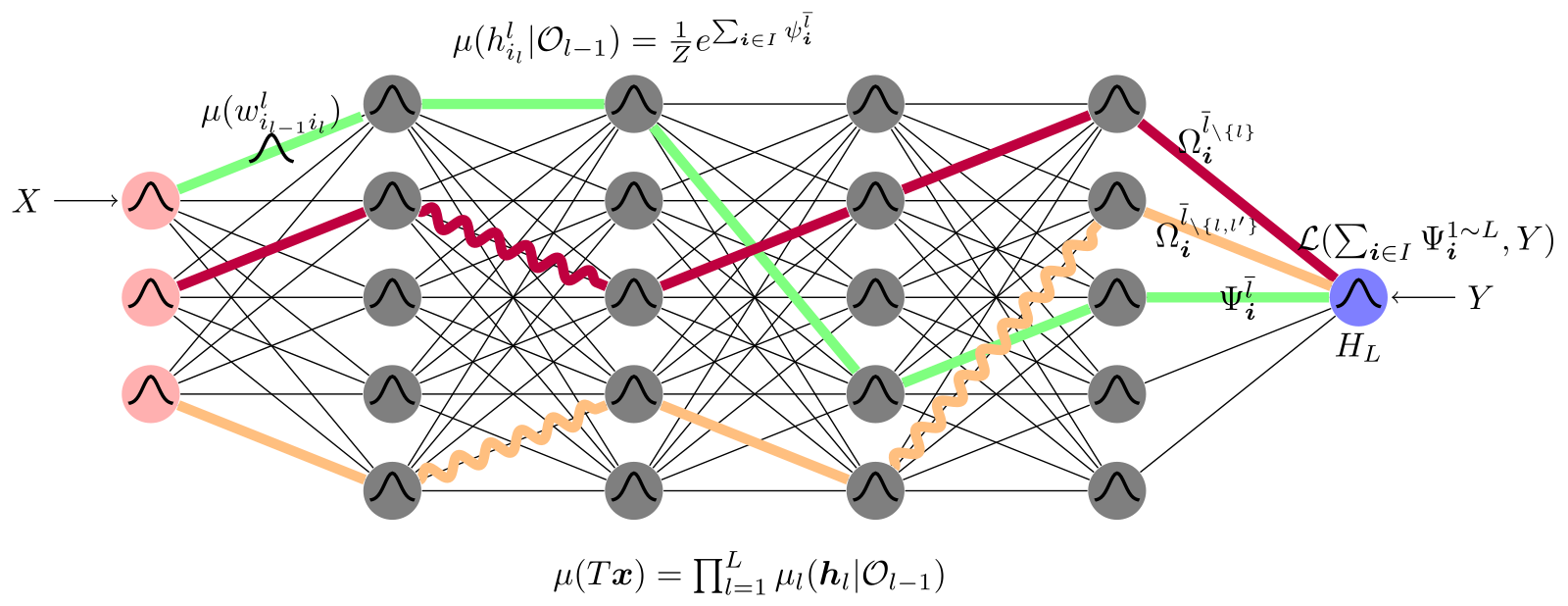
Figure 2: Illustration of the multilayer probabilistic graphical model, the formalism of circuits and the feedback-control loop of DNNs. The learning of Umwelt is through a feedback-control loop composed by hierarchical circuits and the coarse-grained variable computed by the circuits. The loop is graphically illustrated as follows. $l$ denotes layer index. Each node represents a neuronal gate, denoted by $H^{l}_{i_{l}}$ and each edge represents a weight connecting between two neuron gates, denoted by $W^{l}_{i_{l-1}i_{l}}$—neuronal gate is a concept introduced in section II.2, and replaces the activation function in deterministic DNNs with a statistical inference on a random variable supported on $\{0,1\}$. A neuron constituents a gate and the weights connected to the gate. All neuronal gates and weights are random variables—this is emphasized by drawing a bell-shape curve inside each gate, and on the weight at the upper left corner. A path connected gates through weights from left to right (not necessarily the rightmost) is a basis circuit, denoted by $\Psi^{\over{l}}_{\bm{i}}$, that represents the multiplication of all connected random variables, both gates and weights, illustrated as the thick green path; $\overline{l}$ denotes the tuple $(1\ldots l)$, and $1\sim L$ denotes the tuple $(1\ldots L)$—those tuples index basis circuits. The basis circuits with curvy edges (i.e., $\Omega^{\overline{l}_{\setminus\{l\}}}_{\bm{i}}$, $\Omega^{\overline{l}_{\setminus\{l,l^{\prime}\}}}_{\bm{i}}$) represent perturbation of basis circuits induced by perturbations of weights (represented by curvy lines), which are simply basis circuits with the perturbed weights being differentiated out. All basis circuits end with a same gate are arithmetically added together, and are referred as a neuron assembly. Each neuron solves a maximum entropy problem, and thus conditioning on gates in the previous layers, is of an exponential family distribution given by $\mu(h^{l}_{i_{l}}|\mathcal{O}_{l-1})$ at the top, where $\mathcal{O}_{l-1}:=\{X\}\cup\{H_{i}\}_{i\in[l-1]}$ and the energy function is the realization of addition of all basis circuit $\Psi^{\overline{l}}_{\bm{i}}$ connected to it—therefore, all connected gates are statistically dependent with one another. The weights are samples of a prior distribution at the beginning of training. The network $TX$ (i.e., all the weights and gates) is a stochastic system whose law is $\mu(T\bm{x})$ given at the bottom, which factorizes into conditional measures $\mu(\bm{h}_{l}|\mathcal{O}_{l})$ of neurons by layers. The addition coarse-grains over the output of all the basis circuits, and thus computes a coarse-grained random variable; for example, the blue rightmost gate $H_{L}$ is the output of the DNN that estimates the class of the example $X$ perceived by the red leftmost neurons. For each realization (example) of the perceptual signals $X$, the network computes a realization of the coarse-grained variable $H_{L}$. The feedback signal (i.e., labels) $Y$ from the environment (i.e., dataset) is compared against the realization of $H_{L}$ through a surrogate loss function $\mathcal{L}(\sum_{\bm{i}\in I}\Psi^{1\sim L}_{\bm{i}},Y)$, and the discrepancy is back-propagated back to adjust the weights to control the errors. This forward-backward propagation composes one iteration of the loop.

We present a circuit formalism that characterizes the risk minimization of DNNs as a self-organizing informational-physical process where the system self-organizes to minimize a potential function referred as variational free energy [113, 114, 115, 116, 117, 118, 119] that approximates the entropy of the environment by executing a feedback-control loop [8, 41, 71] that is composed by the hierarchical circuits (implemented by coupling among neurons) and a coarse-grained random variable computed by the circuits. The feedback-control loop shall provide the formalism to study the symmetries in DNNs.

Recall that for physical systems, without energy intake, any processes minimize free energy, and free energy could be decomposed into the summation of averaged energy and negative entropy as

$$F=\mathbb{E}_{\mu}[E(\bm{x})]-TS_{\mu},$$ (9)

where with an abuse of notation, $T$ here denotes temperature instead of a DNN. And specifically for the self-organizing process of a physical system, the process dissipates energy and reduces entropy [120]. A DNN is a computational simulation and a phenomenological model of biotic nervous system, and thus it could be appreciated as a model that characterize the informational perspective of the biotic system, and ignores the physical perspective.

More specifically, the maximization of the hierarchical entropy previously approximates the entropy (i.e., $S_{\mu}$) of the environment (dataset). Recall that a loss function in statistical learning [121] is a surrogate function that characterizes the discrepancy between the true measure $\mu(y|\bm{x})$ and the approximating measure $\mu(h_{L}|\bm{x})$. With a logistics risk (i.e., cross entropy), we would have the risk given as

$$S_{\mu(y|\bm{x}),\mu(h_{L}|\bm{x})}:=-\mathbb{E}_{(\bm{x},y)\sim\mu(y|\bm{x})}\left[\log\mu(h_{L}|\bm{x})\right],$$

which is maximization of negative loglikelihood discussed in section II.2. Further notice that, cross entropy could be decomposed into the summation of the KL divergence $D_{\text{KL}}(\mu||\nu)$ and entropy $S_{\mu}$ as

$$S_{\mu(y|\bm{x}),\mu(h_{L}|\bm{x})}=S_{\mu(y|\bm{x})}+D_{\text{KL}}(\mu(y|\bm{x})||\mu(h_{L}|\bm{x})).$$

Thus, the logistics risk is an upper bound on the KL divergence between $\mu(y|\bm{x})$ and $\mu(h_{L}|\bm{x})$ ($S_{\mu(y|\bm{x})}\geq 0$): suppose that at a minimum, KL divergence becomes zero, the cross entropy is the entropy of $\mu(y|\bm{x})$; that is, the entropy of the dataset (environment).

Therefore, the hierarchical maximum entropy problem optimizes the Lagrange multipliers for a variational approximation to the entropy part of the free energy of the environment, and thus could be appreciated as minimizing variational free energy, although the message has been formulated in a rather convoluted way initially under a different context [113].

To analyze this variation free energy minimization process, we develop a formalism of feedback-control loop. However, to begin with, we discuss some background.

1. The macroscopic behaviors—that is, the order at a higher scale—of a self-organizing system are the coarse-grained effect of symmetric microscopic units in the system; for example, for magnetic systems, it is the macroscopically synchronized symmetries of microscopic spins that are perceived as, e.g., magnetic force. Thus, the system could be studied through interaction between the symmetries and the macroscopic behaviors of the system, by typically formulating variables that coarse-grain over the symmetric behaviors of constituent units in the Ising model (through statistical field theory, e.g., techniques such as renormalization groups [122, 58, 59, 60]).

2. However, unlike the homogeneity in physical systems, a biotic system consists of a vast number of heterogeneous microscopic units that interact locally in a hierarchically coupled way against goal-directed feedback signals and induce an emergent macroscopic phenomenon. The spatially and temporally heterogeneous units, and the coupled interaction among units results in the phenomenon that a microscopic change at one scale has implications ramifying across scales throughout the system [69, 70]. Therefore, in biotic systems, the coarse-grained variables are not coarse-grained characterization of a group of units whose higher order coupling could be considered as irrelevant fluctuations and be safely discarded (e.g., field in physics [122, 58, 59, 60]), but are representation of the environment computed by the system itself to capture coarse-grained regularities.

3. Such coupling in biotic systems has been studied through analyzing the feedback-control loop between hierarchical circuits (or simply circuits) in the system and the coarse-grained variables computed by the circuits [48, 49]. The circuits are networks composed by the coupled heterogeneous units that intake feedback (signals from the environment and other units in the system), perform internal computation, and effect actions, and meanwhile compute the coarse-grained variables in the process. For example, in the genotype of an organism, the hypothesis of the organism is encoded as the coupling of heterogeneous genes, and could temporally and spatially regulate the development of the organism. The regulatory process could be studied by analyzing the hierarchical circuits (e.g., gene regulatory networks) that implement feedback-control loops with hierarchically coupled regulatory logic operation and gene expression (which for example, could generate regulatory signals) [43, 44]—hierarchy here refers to, for example, the animal body development determined by gene regulatory networks, where each phase of the development encoded by the genes has beginning, middle and terminal stages, and later events recursively refine the body parts developed in early events [43]. A more detailed introduction to the methodology in theoretical biology is given in supp. D B.

Thus, first we develop a circuit formalism. The exponent in eq. 6 could be rewritten as

$$\sum_{\bm{i}\in I}X_{i_{0}}\Psi^{\wedge 1\sim L\wedge}_{\bm{i}},$$ (10)

where

$$\Psi^{\wedge 1\ldots L\wedge}_{\bm{i}}:=\prod_{l=1}^{L-1}W^{l}_{i_{l-1}i_{l}}H^{l}_{i_{l}}W^{L}_{i_{L-1}i_{L}},I=\overrightarrow{\otimes}_{l\in\mathbb{L}}[n_{l}],$$ (11)

and we have used upper case notations instead of lower case because all the variables there are random variables—the exponent is the realization of those random variables: eq. 6 is the law of gates conditioned on weights and gates of previous layers, and the law of weight matrices are symmetric at initialization, but would change after training starts. We call $\Psi^{\wedge 1\ldots L\wedge}$ a basis circuit, and the wedge symbol is also part of the formalism that denotes the circuit is missing an input or an output—$X_{i_{0}}$ is written as the input explicitly and thus $\Psi^{\wedge 1\ldots L\wedge}_{\bm{i}}$ has a wedge symbol on the left. For convenience, we also write $\Psi^{\wedge 1\ldots L\wedge}_{\bm{i}}$ as $\Psi^{\wedge 1\sim L\wedge}_{\bm{i}}$. In addition, a basis circuit is defined recursively, and thus a segment of basis circuit is also a basis circuit: for example,

$$\Psi^{\wedge 1\ldots l^{\prime}\wedge}_{\bm{i}_{:l^{\prime}+1}}:=\prod_{l=1}^{l^{\prime}-1}W^{l}_{i_{l-1}i_{l}}H^{l}_{i_{l}}W^{l^{\prime}}_{i_{l^{\prime}-1}i_{l^{\prime}}},$$

where $l^{\prime}<L$. Further notice that eq. 10 is the coarse-graining/addition of a large number of basis circuits, and we refer it as an assembly.

Under the circuit formalism, the risk minimization of a DNN $T(X)$ could be written as

$$R =\mathbb{E}_{(X,Y)\sim\mu}\left[\max(0,1-YT(X)\right]$$ (12)

$$=\mathbb{E}_{(X,Y)\sim\mu}\left[\max(0,1-Y\sum_{\bm{i}\in I}X_{i_{0}}\Psi^{\wedge 1\sim L\wedge}_{\bm{i}})\right],$$

where we have used hinge loss as a concrete example to illustrate, and in this case the output $T(X)$ of a DNN is simply the coarse-graining of basis circuits—if logistics risk is used, the coarse-graining is the logit and still needs to pass through a sigmoid function to become the output. Then, the dynamics of the self-organizing process of a DNN is a feedback-control loop given as the iterative process

$$\frac{d\bm{\theta}}{dt}=-\eta\nabla_{\bm{\theta}}R,$$ (13)

where $\eta$ is a scalars that scale the gradient $\nabla_{\bm{\theta}}R$ and is called as step size, or learning rate in the literature, and $\bm{\theta}$ denotes all the trainable parameters of a DNN. The loop characterizes a dynamical process that executes a loop described as follows: first, the circuit composed by neurons represents a hypothesis that computes a prediction of a coarse-grained random variable $H_{L}$; second, a surrogate risk that measures the discrepancy between the prediction and the observed valued of the variable ($Y$, feedback signals) from the environment/dataset; third, the circuit self-organizes according to gradient/feedback back-propagated from the feedback signals (the derivative of risk w.r.t. $T(X)$) at the top-layer neuron; lastly, the process goes back to the first step. The preceding concepts are illustrated in fig. 2.

II.4 Adaptive symmetries in the feedback-control loop

Self-organization is a transdisciplinary concept that tries to characterize both the physical and biotic systems [105, 9], and has the problem of ambiguous definitions [106, 107, 108, 109, 110, 111, 112]. The self-organization of magnets given in section II.3 is more precisely characterized as a symmetry-breaking process: as the temperature decreases, the free energy of the system decreases, and the system self-organizes and breaks symmetries known as the translation and rotation symmetry; the breaking of rotation symmetry leads to the alignment of the spins’ spinning direction, which collectively manifests as the magnetic field; and the breaking of translational symmetry results in the phenomenon that magnetic fields with varied strength exist at different spatial locations of the system. Collectively, the breaking of the two symmetries is known as replica symmetry breaking [123, Chp 3]. To clarify, we have described the symmetry breaking of a particular type of magnets known as spin glasses, and the spin glasses would be the example to illustrate concepts from now on because some extraordinary similarity exists between DNNs and spin glasses, which we would intermittently discuss throughout this work. Perhaps marvelously, the self-organization of DNNs could also be characterized as a symmetry-breaking process, and in the following, we characterize a symmetry that we refer as circuit symmetry.

II.4.1 From conservative-symmetry in physics to adaptive-symmetry in biology

To begin with, we introduce the foundational role that symmetries play in physics. The symmetries in physics are formalized as symmetry groups in mathematics. Symmetry groups formalize invariants of physical systems that constituent the fundamental concepts to understand these systems [36, 37]:

1. symmetries construct objectivity by identifying observables that are stable at a spatial and time scale of human perception and thus could be measured by instruments; such stable behaviors are concentration-of-measure phenomena manifesting over time, and referred as ergodic states [124] of the system that are related by symmetric transformations that conserve the free energy;

2. the breaking of symmetries is associated with the change of a system’s stable behaviors, and thus characterizes the dynamics of the system;

3. and the hypotheses derived from these mathematical invariant and the experimentally validation of the hypotheses through measurements on the observables constitute the fundamentals of the science of the system.

For example, at a high temperature the rotation symmetry of the spins are the stable invariant that characterizes the behaviors of the system—rotation of the spins conserves the free energy. Energy dissipation of the system decreases free energy, and thus breaks the rotation symmetry. The breaking of the rotational symmetry characterizes the dynamics of the system. The dynamical process can be experimentally observed by measuring the magnetization, and the spin glass order parameters. Therefore, symmetries formalizes the conserved behaviors (e.g. free energy in a spin glass) of a physical system when no external factors (e.g., energy) are influencing the system, in this regards, symmetries in physical are conservative symmetries. A more detailed introduction is given in supp. D A.

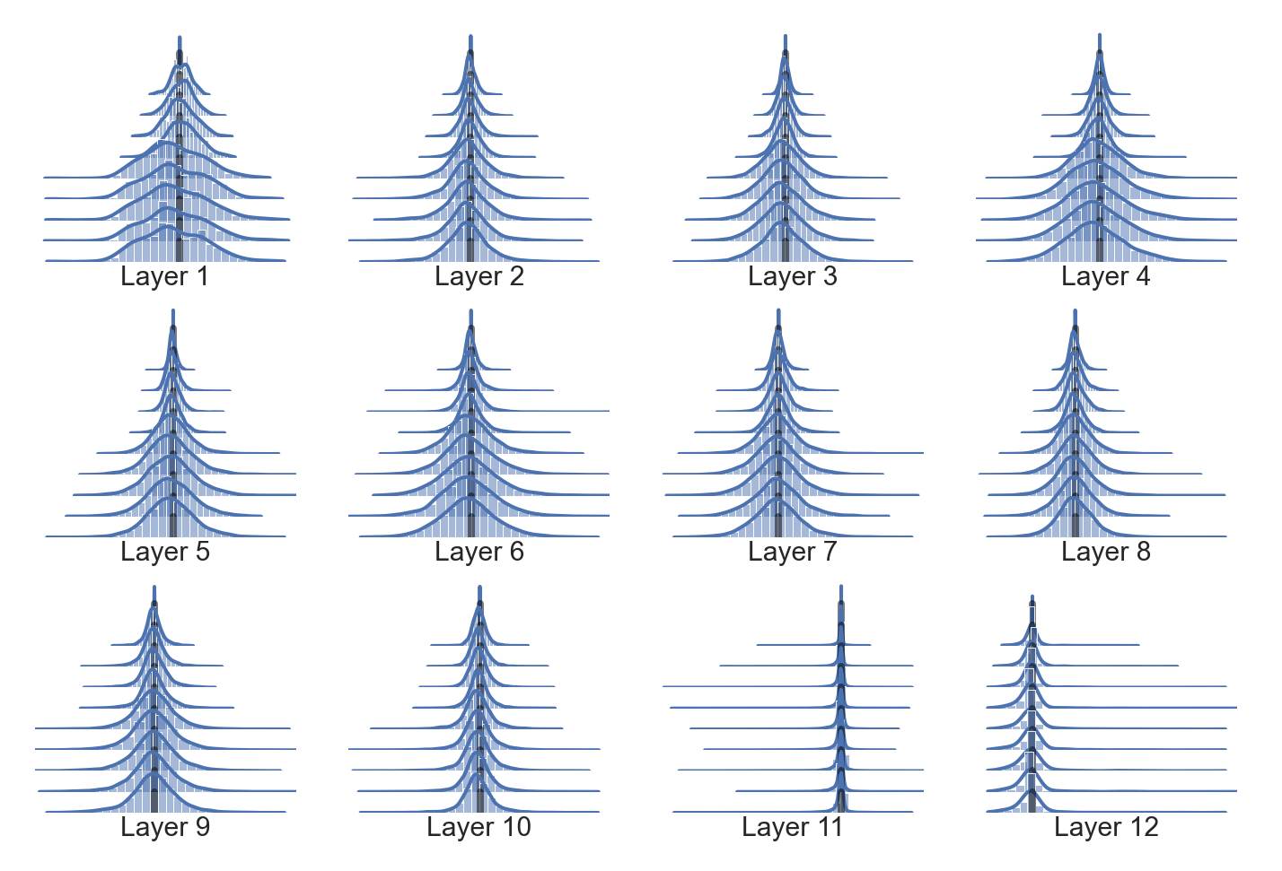
(a) Mixture of intact and broken weight symmetries throughout DNN training. The figure has $12$ subplots that each plots the weights’ distribution at a layer of the DNN in the experiments throughout training—the DNN has $12$ layers. Each subplot has $10$ histograms plotted from the top to the bottom, and plots the distributions at epoch $0,10,20,30,40,100,160,200,260,300$, respectively. The black line at the center of each ridgeline graph is the $y$-axis. The blue lines are the smoothed histograms obtained by smoothing the frequency with a Gaussian kernel.

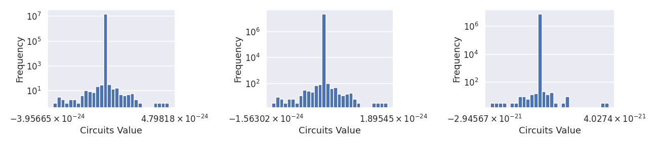
(b) Circuit symmetries of basis circuits, and perturbation of basis circuits of order $1,2$ at the beginning of DNN training. The three plots from left to right are the histogram of basis circuits (which compute the output of a DNN), histogram of perturbations of basis circuit of order $1$ (which compute the gradient of a DNN), histogram of perturbation of basis circuit of order $2$ (which compute the Hessian of a DNN). The basis circuits are sampled from all possible basis circuits uniformly at initialization. Though the number of circuits sampled is only a varnishingly small fraction of all possibles circuits, the symmetry is consistently observed for dozens of samples in experiments that are not shown here.

Figure 3: Microscopic adaptive symmetries in a DNN whose specification is introduced in section I.1.3. Each weight $W^{l}_{i_{l-1}i_{l}}$ (an edge in fig. 2) is of a law that is symmetric w.r.t. $y$-axis at the beginning of the training, and fig. a shows that such weight symmetries only slight skews throughout training, implying the majority of the weight symmetries do not break during training. A basis circuit (a path in fig. 2) is the multiplication of neuronal gates and weights, and thus the weak correlation among gates—as a result of the fact that each gate is connected to a large number of neurons—and weight symmetry are theoretically found (through a theorem) to induce a composite symmetry of basis circuits, referred as the circuit symmetry. Circuit symmetries at the beginning of the training are experimentally shown in fig. b. A basis circuit of circuit symmetry is of equal probability to contribute to the coarse-grained variable in the feedback-control loop, positively (e.g., detecting a nectar-making flower) or negatively; and in response to the feedback signals (labels), circuit symmetries would break to decrease the errors (e.g., of detecting flowers). The symmetries break heterogeneously: the broken symmetries encode information about the environment/dataset, and the intact symmetries maintain adaptability to reduce further information perturbations (errors) of novel examples.

However, in biotic systems, symmetries conserving free energy is continually being broken and no symmetries of conservation exist that constituent fundamental concepts to understand biotic systems; instead, the invariant of variants, might be a fundamental concept [38, 47, 52]. In this work, we formalize a stable invariant of variants as adaptive symmetry or symmetry of adaptation. We introduce the concept of adaptive symmetry as follows.

1. The symmetry is not like the symmetries of conservation in physical systems that are induced by the preference of units to a certain configuration to minimize free energy, but is a symmetry of adaptation: the system has the capacity to process the novel information—that is, to adapt—by posing in states where symmetric possible directions to adapt could be adopted, which in turn is induced by the complex cooperative interaction among the heterogeneous units in a biotic system; and the symmetric states would break in response to random fluctuations and external feedback signals [45, 68], and thus is also a typical self-organizing process. The breaking of such symmetries results in functional diversification on every scale, from molecular assembliers, to subcellular structure, to cell types themselves, tissue architecture, and embryonic body axes [45].

2. For example, the cell specification in the embryonic differentiation could be conceptualized as a symmetry breaking process: from a symmetric state where an embryonic cell has multiple ways to adapt, in response to the feedback signals regulated temporally and spatially by gene regulatory networks [43, 44], the cell breaks the symmetry, and specifies into more specialized types of cells.

3. In the lifespan of a biotic system, the symmetries and broken symmetries coexist, and might be a way to characterize structural stability and adaptability of life [37]: for example, despite an organism was developed by breaking a sequence of symmetries since the embryonic stage, immune cells could still break symmetries and differentiate into specialized immune cells in response to specific pathgens.

The study of biological symmetry breaking is still an on-going scientific efforts; the relation between biological symmetry and conservative symmetries in physics has not been fully understood, and a formalism comparable to the Noether’s theorem in physics is yet to be formulated [37, 61]. We shall provide some examples to speculatively discuss the interaction between conservation symmetries in physics, and adaptive symmetries in biology when we discuss the related works that apply conservative symmetries to DNNs in supp. A C. And again, a more detailed discussion is given in supp. D A.

II.4.2 Circuit symmetry in DNNs

Each basis circuit (introduced in II.3) is a microscopic feedback-control loop that contributes to the computation of the coarse-grained variable $H_{L}$. We identify an adaptive symmetry, referred as circuit symmetry, of the basis circuits that characterize the phenomenon that is of equal probability to contribute to the coarse-grained variable positively or negatively—that is, for example in binary classification problem, to contribute positively to classify the pattern as $1$ (positive example), or negatively to classify the pattern as $0$ (negative example). This circuit symmetry would break to change the coarse-grained variable positively or negatively, in response to the feedback signals, i.e., labels of the data. We introduce the symmetry as follows, and a more rigorous formalism and further details are given supp. B E.

A statistical-physical system is characterized statistically as an ensemble of possible states where the system could be in. And symmetries in physics characterize equivalent states in the sense of free energy, and thus the probability of a system to stay in these states. Thus, at equilibrium, symmetries in statistical physics characterize the equivalence among ergodic states over a long-time (compared with thermodynamic timescale).

In contrast, circuit symmetry also characterizes certain equivalence among possible states realized from an ensemble of all possible states, but there are no transitions among these states in the sense of ergodicity—such a symmetry has been referred as stochastic symmetries in the context of complex networks [125, Chp 6]. In addition, equivalence of circuit symmetry is not in the sense of free energy, but of adaptability.

An adaptive symmetry, referred as weight symmetries, exists in DNNs; and the cooperative breaking of such symmetries would induce system-wide ordered, or macroscopic, behaviors of DNNs. Operationally, the weight symmetries simply characterize the phenomenon that each weight of a DNN is sampled/realized from a random variable with a symmetric law. Furthermore, note that each weight is realized from a independent random variable. Such individualized symmetries imply that the symmetries could be broken in a heterogeneous way—which we refer as heterogeneous symmetries—as in the biotic systems, where macroscopic symmetries are composed by heterogeneous units whose symmetries would break in response to the local, transient, even noisy feedback signals each unit received, and whose symmetry breaking cooperates to form stable system-level asymmetries [45]. For a large network, only a subset of weights’ symmetry would break throughout training to encode information, and statistically, the weight symmetry still holds for the majority of the weights. This could be seen in fig. 3a, where we could see that although the weight distributions gradually skew as training progresses, they are still approximately symmetric w.r.t. $y$-axis throughout the training.

Weight symmetries induce a composite symmetry that are referred as circuit symmetry. Recall that feedback-control loop of DNNs is composed by hierarchical basis circuits and the coarse-grained variable, and the coarse-grained variable is computed by a neuron assembly that is the addition of basis circuits. Thus, each (basis) circuit in the loop is a microscopic feedback-control loop composed by neurons and the weights connecting neurons. Correspondingly, weight symmetries induce the composite circuit symmetry. Because weight symmetry is a heterogeneous symmetry, and thus circuit symmetry is also a heterogeneous symmetry. As a result, the circuits in a DNN could be of broken symmetry in only a subset of all circuits, and the system is in a state where intact and broken circuit symmetries coexist. This phenomenon is a concentration-of-measure phenomenon and is characterized as a probability bound in a theorem given in supp. B E 5. Informally, for any basis circuits whose weights are of weight symmetry,

$$\mu(\psi^{1\sim L\wedge}_{\bm{i}})\approx\mu(-\psi^{1\sim L\wedge}_{\bm{i}}).$$ (14)

We also plot the histograms of basis circuits at the beginning of the training in fig. 3b for demonstration: we only plot the histograms at initialization because once the training begins, the statistical behaviors of basis circuits that result from random initialization are broken, and it is difficult to identify basis circuits that are of circuit symmetry among the exponential number of basis circuits without sophisticated efforts, which would be a digression; instead, we simply uniformly sample basis circuits at initialization for demonstration, and circuit symmetries could be seen through such uniform sampling. The figure actually presents three types of basis circuit, and in the current stage, we have not explained in details the perturbations of basis circuits, which compute derivatives of output of a DNN, and they could be understood simply as basis circuits. As could be seen from fig. 3b, the law of basis circuits are symmetric—the output of a DNN, the gradient, the Hessian (i.e., neuron assemblies), are simply the addition of the output of these basis circuits, respectively.

II.4.3 Statistical assembly methods

Recall that in section II.4.1, we introduce that symmetries in physics identify observables that characterize the coarse-grained/macroscopic behaviors of the system. These coarse-grained observables are typically self-similar to the microscopic behaviors as a result of symmetries, and are calculated through renormalization over symmetry groups—that is, the renowned renormalization group technique. Further recall that the coarse-grained variables (i.e., assemblies) computed by a DNN are the addition basis circuits, and the addition is actually over symmetry groups. A core of this work is to show that coarse-grained behaviors of basis circuits that are self-similar to the behaviors of basis circuits also exist for DNNs; in other words, the coarse-grained effect of the microscopic adaptive symmetry would manifest as a macroscopic/coarse-grained adaptive symmetry of DNNs. The analysis could be appreciated as a methodological synthesis of ideas from Statistical Learning Theory [121] and the Statistical Field Theory [91] in physics. We refer the method as the statistical assembly method. In this subsection, we first introduce the statistical-field approach and the statistical-learning approach, and discuss their limitations, and then we introduce the statistical assembly method.

The statistical-mechanics approach to study DNNs have a long history [126, 127, 128, 31], however, the application of this approach typically requires homogenization of data and models, and thus the ensued analyses are away from practical settings. More specifically, in physical systems, a field is a coarse-grained characterization of a collection of particles, and it is a good formal model of the particles’ collective behaviors because the disorganized interaction among particles, unraveled through a timescale orders of magnitude larger than the thermodynamic timescale, results in statistically stable, homogeneous behaviors of this collective. A typical example would be the mean-field models, which we refer to supp. D D for a review. As a result, statistics of the collective makes a coarse-graining for analysis, which is also known as effective theory in physics. And more particularly, the behaviors of particles could be characterized as Gaussian fields/distributions, and thus the many-body interaction of particles are high-dimensional Gaussian integrals. Therefore, to apply the statistical field method to neural networks, the data and interaction among neurons need to be homogenized [126, 127, 128, 31, 129, 130], and the setting is away from practical setting [31]; for example, the input data are assumed to uniformly sampled from a hypersphere—more related works could be found in the related-works discussion in supp. A D 4, where the works that do finite-width correction to infinite-width assumption typically make such homogeneous assumptions over data.

Meanwhile, the statistical learning theory is a revolution in statistics that does not requires restrictive assumptions, such as those in analyses from the approach of statistical mechanics, however, the theory was developed to analyze relatively simple models, and the analyses do not generalize straightforwardly to complex models in high dimensional setting like DNNs—currently, complex models on high dimensional data like DNNs lie in a “no man’s land” between efficient linear methods on high-dimensional data with strong regularities in the sense of concentration-of-measure phenomena, and low-dimensional data with efficient complex nonlinear methods [72]. More specifically, the utilities of the statistical-learning analysis lie in characterizing worst-case behaviors that are close to the practical behaviors in the sense that the former could qualitatively characterize the latter—and in many cases, the worst case behaviors could prescribe quantities that control generalization; this resembles control parameters in statistical physics. Concretely, a primary goal of learning theory is to characterize the generalization of a hypothesis/classifier through an upper bound. The upper bounds obtained are worst case behaviors of samples. In simple models, the behaviors characterized by the bounds are close to practical behaviors, in the sense that, for example, the bounds can qualitatively characterize the generalization ability of the hypothesis by identifying quantities (e.g., margins of support vector machine (SVM), or margins [131], distance from initialization [132], singular values [133] of DNNs) that qualitatively characterizes the generalization ability. More concretely, with the margins of SVM as an example, though each training example has a margin of its own, the bounds are characterized by the smallest margin among all training examples. Consequently, the generalization errors are over-estimated, and the utility of the bound is to identify the margin as a qualitative characterization of generalization, and in practice, the margins of all examples would be intentionally maximized to achieve better generalization. However, as probability bounds, their values are typically much larger than $1$—the looseness of generalization bounds in the context of DNNs has been discussed [23, 131]. And to reach descriptive or prescriptive bounds, extra care is needed to identify worst-case behaviors that are close to practical behaviors. Otherwise, the intuition obtained from simple models could be misleading: for example, the bias-variance trade-off is based on analysis of simple models, and for complex models like DNNs, the behaviors of generalization are not exactly the same with the broad-stroke bias-variance trade-off, and manifests as the double descent phenomenon [134, 135].

In this work, we synthesize the two approaches through symmetries: we do not make restrictive assumptions on data distributions as works under the statistical-mechanics approach do, which is achieved by analyzing worst-case behaviors similar to works in statistical learning theory, and that we do calculate many-body interaction in the system, but at the granularity of assemblies that characterize hierarchical many-body interactions. This approach could be appreciated biologically: given the unknown in an environment, a strategy for an organism to prevent coincidental survival risk is to hoard a reservoir of backup plans to stay far away from vulnerable situations. More specifically, Carleo et al. [31] speculate that the statistical-mechanics approach and statistical-learning approach are complementary once we understand the key conditions under which practical cases are close to worst cases. In DNNs, the basic units are not homogeneous particles, but heterogeneous basis circuits that each has its particular behaviors. The coarse-grained behaviors of the basis circuits are formalized as assemblies that also each has its own particular behaviors. And it seems that it is only analytically amenable to analyze the extreme case behaviors of all assemblies—this is a trade-off made between verisimilitude and analytical tractability. As a result of this trade-off, the quantitative characterized achieved would be significantly lower or higher (depending on whether a lower or an upper bound is taken) than the actual behaviors of the system. Meanwhile, circuit symmetry formalizes the repetitive/invariant behaviors across assemblies. Such invariance makes the extreme-case behaviors close to the practical behaviors. Consequently, although the quantitative characterization in this work does not exactly characterize the behaviors of DNNs, it does so qualitatively, as in the approach of statistical learning theory. Meanwhile, the extreme-case characterization is calculated from extreme-case behaviors of many-assembly interaction up to arbitrary order, and thus it is also a statistical characterization resembling that of the statistical field theory. For conceptual clarity, we refer this method as statistical assembly methods, to clarify both the difference and the similarity with the statistical learning theory and statistical field theory.

The rest of this work is the application of the method to study the coarse-grained effect of circuit symmetries that leads to a phase of DNNs: the correlations among assemblies of all orders are calculated, and when a DNN is hierarchically large, a concentration-of-measure phenomenon manifests where the eigenspectrum of a DNN’s Hessian could be characterized by a self-consistent matrix equation, and that qualitatively characterizes practical behaviors.

II.5 Order from fluctuations, or order from adaptive symmetry

The circuit symmetry introduced in section II.4 is a heterogeneous symmetry, which implies, as we have explained in section II.4, that during the self-organizing of DNNs, intact and broken symmetries could coexist: broken symmetries encode information about the environment/dataset, and manifest as complex functional structure; the intact symmetries maintain the ability to further reduce information perturbations (training errors). Therefore, the self-organizing process is a process where circuit symmetries are continually being broken. Further recall that circuit symmetries characterize the symmetric distribution/perturbations of (output of) basis circuits around zero. Therefore, the preceding self-organization (risk minimization) is a salient “order from fluctuations” phenomenon that characterizes self-organization, and the order emerges from disorder in circuits by selective (positive, or negative) feedback signals that breaks the circuit symmetries. However, to further study such a symmetry-breaking process, we need to clarify the concept of order in DNNs next, and a more rigorous presentation and further details are given in supp. B F.

II.5.1 Order in physics and self-organization

To begin with, we introduce the concept of order in physics. In section II.4, we have explained that symmetries identify observables that are coarse-grained effect of symmetries. Intuitively, for a system consisting of microscopic units to manifest behaviors that could be consistently observed at a macroscopic scale, a synchronization/cooperation of a large number of the microscopic units needs to somehow occur. And the synchronization results in self-similarity between the microscopic units and the macroscopic/system-wide behaviors. And in physics, such a macroscopic behavior is referred as the order of a system. The self-organization of a physical system is the process where the constituent units synchronize to transit from one macroscopic behavior to another. To give an example in daily life, snowflakes also self-organize: when temperature falls, the rotational symmetry is broken into a six-fold symmetry, and macroscopically, and we observe the flower-like shape of the snowflakes. The shape is the (macroscopic) order of water molecule system emerges from disorder at high temperature, and the temperature is the control parameter of the process.

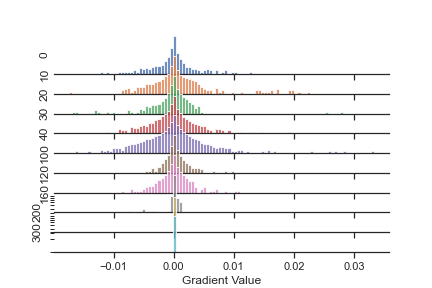
(a)

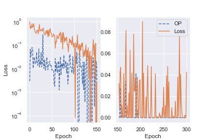
(b)

Figure 4: Adaptive symmetry of, or coarse-grained effect of circuit symmetries on gradients, and the dynamics of the plasticity order parameter. Gradients are perturbation of neuron assemblies of order one. And they are experimentally found to be self-similar to the circuit symmetries of perturbation of basis circuits of order one throughout training (shown in fig. a), implying that the coarse-graining of the mixture of intact and broken circuit symmetries manifests as adaptive symmetries at the assembly level. The further coarse-graining of gradients by adding up the square of gradients leads to nonzero squared norm of the gradient vector, and characterizes that whether the coarse-grained effect of circuit symmetries is capable of breaking to decrease the errors (measured by empirical risk) of the prediction of the coarse-grained variable (i.e., $H_{L}$ in fig. 2) computed by the network (shown in fig. b). Thus, according to the epistemology of physics, the squared norm of gradient vector is referred as the plasticity order parameter to quantitatively characterize the order of DNNs. (a) Adaptive symmetry of gradients throughout DNN training. The figure plots the distributions of gradients throughout training, where the numbers on the left of the plot are the epochs where the gradients are computed. (b) The transition of plasticity order parameter and empirical risk from nonzero to zero during DNN training. The curve denoted by OP is the step-size rescaled plasticity order parameter throughout training. The curve denoted by Loss is the training loss/risk throughout training. The plot is divided into two subplots because we plot the first 150 epochs in logarithmic scale to emphasize that the scaled order parameter decreases roughly by the same rate with the loss, and is approximately an order of magnitude smaller than the loss; and in the second subplot, we need to revert back to the normal scale because the loss is too small and as such, the statistical fluctuations are amplified in logarithmic scale, and obfuscate the information that both the order parameter and the loss are close to and oscillate to zero.

The order described previously is a macroscopic behavior of a physical system at equilibrium. And when a system is referred as self-organizing, it tends to describe a non-equilibrium system. And the order of a self-organizing system typically refers to a stable dynamic behavior, for example, a dissipative structure such as the Rayleigh-Bénard convection, which emerges from stable fluctuations caused by energy input/gradients. Such dynamics is summarized as “order from fluctuations” by Prigogine [120], “order from noise” by von Foerster [100], or “order from chaos” by Kauffman and Kauffman [136]. The circuit-symmetries breaking presented in section II.4 is exactly such a process: each basis circuit fluctuates (is of probability measure distributed) symmetrically against $y$-axis to break its symmetry to decrease the error of novel examples.

II.5.2 Order of DNNs

We characterize the order of DNNs, by studying the coarse-grained effect of circuit symmetries introduced in section II.4. We shall present a macroscopic adaptive symmetry that characterizes the order of DNNs: a self-similarity between the macroscopic (i.e., neuron assemblies) and the microscopic (i.e., basis circuits composed by neurons).

First, we present an order parameter of DNNs. In statistical physics, the order of a system is formally and quantitatively characterized by order parameters that coarse-grain the symmetric behaviors of microscopic units, e.g., the magnetization order parameter of magnets. The order parameter of a system is typically identified by examining the elementary excitation [35, Chp 9.3] of symmetries in the system in response to perturbations: the magnetization order parameter of a ferromagnet is the first-order excitation of magnetic spins in response to an external magnetic field, or colloquially, putting a magnet close to magnetic field, the collective behaviors of the units in the magnet would induce a repulsive or attractive force, depending on the polarity—a review of these concepts in physics is given in supp. D C. The external perturbations of a DNN are simply novel examples of nonzero errors, and we examine the elementary excitation of DNNs in response to novel examples and formally define the first order excitation (i.e., the square of gradient norm) as the order parameter of DNNs,

$$||\nabla_{\theta}R||_{2}^{2}=\sum_{l=1}^{L}\sum_{i_{l-1}=1,i_{l}=1}^{n_{l-1},n_{l}}\sum_{\bm{i},\bm{i}^{\prime}\in I^{\setminus\{l-1,l\}}_{i_{l-1}i_{l}}}\Omega^{\overline{l}_{\setminus\{l\}}}_{\bm{i}}\Omega^{\overline{l}_{\setminus\{l\}}}_{\bm{i}^{\prime}},$$ (15)

where $\overline{l}$ denotes $(1\ldots L)$, $\Omega^{\overline{l}_{\setminus\{l\}}}_{\bm{i}}$ denotes

$$X_{i_{0}}\Psi^{\wedge 1\sim l-1\wedge}_{\bm{i}_{:l}}H^{l-1}_{i_{l-1}}H^{l}_{i_{l}}\Psi^{\wedge l+1\sim L\wedge}_{\bm{i}_{l:}}\mathcal{L}^{\prime}(\cdot),$$ (16)

which is the first derivative of basis circuit given at eq. 11 that intakes a datum $X_{i_{0}}$ at the bottom layer, and a derivative $\mathcal{L}(\cdot)$ at the top layer; and $I^{\setminus\{l-1,l\}}_{i_{l-1}i_{l}}$ denotes

$$\overrightarrow{\otimes}_{\{p\in\overline{l}|p<l-1\}}[n_{p}]\otimes\{i_{l-1}\}\otimes\{i_{l}\}\overrightarrow{\otimes}_{\{q\in\overline{l}|q>l\}}[n_{q}];$$

that is, $[n_{l-1}],[n_{l}]$ are substituted by single element sets $\{i_{l-1}\},\{i_{l}\}$, respectively, in the consecutive Cartesian products that previously composes the index set $I$ of basis circuits in eq. 11. We refer $\Omega^{\overline{l}_{\setminus\{l\}}}_{\bm{i}}$ as first order perturbations of basis circuits induced by weights—an illustration is given in fig. 2—and eq. 16 the plasticity order parameter, which characterizes whether a DNN is able to continue to absorb information perturbations, or in other words, to decrease the errors of novel examples.

Remarkably, under the circuit formalism, the plasticity order parameter is symbolically equivalent with the spin glass order parameter. Recall that the spin order parameter of spin glasses is

$$\propto\mathbb{E}_{\rho(\bm{\sigma})}[\sum_{ij}\sigma_{i}\sigma_{j}],$$ (17)

where $\sigma_{i},i\in[n]$ denotes spins, and $\rho$ denotes the law of the spins $\bm{\sigma}$—it could be derived by taking the first order derivative of free energy (i.e., the elementary excitation), and the derivation is given in supp. D C for interested readers. Equation 15 resembles symbolically to eq. 17 if we merge the three summation symbols into one big symbol. The resemblance is also semantically informative to understand the coarse-grained symmetries of DNNs. Recall that in section II.3, we interpret the risk minimization of DNNs as a variational-free-energy-minimization process where the uncertainty of the coarse-grained variable that detects macroscopic patterns is minimized by a feedback-control loop between the coarse-grained variable and the hierarchical circuits computing the variable. The plasticity order parameter is the quantified uncertainty reduced in one step of the risk minimization, and is a coarse-grained variable that coarse-grains the change in the neuron circuits that induces the uncertainty reduction. A spin glass self-organizes to align spins at a macroscopic scale; thus order manifests when the spins align. A DNN self-organizes to reduce uncertainty in pattern recognition; thus order manifests when the basis circuits pose to reduce uncertainty. The coarse-graining of spins computes the degree of alignment/order that induces magnetic force/potential in response to external magnetic field, whereas the coarse-graining of the output of circuits computes the potential reduction of uncertainty in response to information perturbations. Both spins and basis circuits make binary choices that increase or decrease the order parameter, though the binary choices of circuits result from the hierarchical coupling of many neurons.

Notice that the differentiation only removes one weight from each basis circuit, and thus if the weight symmetry still holds for the rest of the weights, circuit symmetry still holds. A self-similarity (of adaptive symmetry) between gradients and first-order perturbation of basis circuits is experimentally observed in fig. 4a: each entry of the gradient is a coarse-grained observable of perturbation of basis circuits (i.e., neuron assemblies),

$$\sum_{\bm{i}\in I^{\setminus\{l-1,l\}}_{i_{l-1}i_{l}}}\Omega^{\overline{l}_{\setminus\{l\}}}_{\bm{i}},l=1\ldots L,i_{l-1}=1\ldots n_{l-1},i_{l}=1\ldots n_{l};$$

they are observed to be symmetrically distributed against $y$-axis, and gradually converge to zero during the training of a DNN. Correspondingly, as could be seen in fig. 4b, the plasticity order parameter gradually transits from nonzero to zero, and reaches zero when the empirical risk is zero—recall that in physics, the order parameters transits from zero to nonzero (or, vice versa) during phase transitions.

II.6 Plasticity phase, extended symmetry breaking, and benign pathways on the risk landscape

In section II.5, we explained that the order of a system is the macroscopic behaviors of the system that are the coarse-grained effect of stable symmetries in the system, and are quantitatively characterized by order parameters. And thus different stable symmetries would induce distinctive macroscopic behaviors, and such distinctive behaviors are referred as phases of the system. In this section, we shall characterize a phase of DNNs, which we refer as the plasticity phase, where a coarse-grained adaptive symmetry exists that is self-similar to the circuit symmetry of basis circuits. Meanwhile, the phase is both a phase of a DNN, where the DNN could continually decreases risk, and an extended symmetry-breaking process, where the symmetries are continually being broken during the self-organizing process. As a result, the benign pathways (that lead to zero risk) exist, and thus suggests an explanation of the marvelous optimization power of DNNs in practice. We introduce the phase in the following, and a more rigorous presentation and further details are given in supp. B G.

II.6.1 Phase space in physics

To begin with, we clarify the concept of phase space in physics. Recall that in section II.4, we explained that symmetry groups formalize invariants of physical systems that constituent the fundamental concepts to understand these systems. A formalism that systematically organizes the concepts is the phase space: in statistical physics, a phase space is a mathematical space whose coordinates are control parameters, and order parameters are functions defined on the space that uniquely determine the system’s behavior of interest [38]—both the control and order parameters are observables identified by symmetries. Further recall that in section II.5, we explained that order parameters characterize the system’s excitation in response to perturbations. When the energy perturbation is sufficiently large or the system is at critical regimens, the symmetries would be broken, and the system would undertake a phase transition from a phase with one set of stable symmetries to another. The phase transitions—that is, symmetry breaking—are singular points of the function where the order parameter singularly changes from one value to another. For example, the phase space/diagram of spin glasses is a Euclidean space (cf. figure 2.1 in Nishimori [123]) whose coordinates are control parameters (e.g., temperature); and order parameters (e.g., spin glass order parameter) are functions defined on the space that uniquely determine the system’s behavior of interest (i.e., paramagnetic, ferromagnetic, or glassy phase). Stable rotation and translation symmetry of magnetic spins in a spin glass is referred as the paramagnetic phase, and is quantitatively characterized by zero magnetization order parameter. The phase transitions from the paramagnetic phase to the ferromagnetic phase—that is, rotation symmetry breaking—are singular points of the (order parameter) function where the magnetization order parameter singularly changes from zero to nonzero. More detailed review of the concepts is given in supp. D C.

II.6.2 Hypothesis on a phase of DNNs with stable circuit symmetries

Following the epistemology of physics, to understand the symmetry breaking of DNNs, we investigate the phases of DNNs. We hypothesize that the consistent adaptive symmetry of gradients experimentally observed in section II.5.2 is a phase of DNNs, i.e., a stable macroscopic behaviors of DNNs. More specifically, recall that in section II.4, we introduce that because circuit symmetry is a heterogeneous symmetry, the circuits in a DNN could be of broken symmetry in only a subset of all circuits, and the system is in a state where intact and broken circuit symmetries coexists. And in section II.5, we introduce the experiments that observe a macroscopic adaptive symmetry self-similar to adaptive symmetry of basis circuit (i.e., circuit symmetry): the gradients as coarse-grained observables of perturbation of basis circuits are symmetrically distributed against y-axis throughout the training of a DNN. Therefore, we might hypothesize that throughout the training, the DNN is in states where circuit symmetries stably exist (along with broken circuit symmetries) to manifest adaptive symmetry at the level of assemblies (e.g., symmetry of the gradient distribution). And the adaptive symmetry of assemblies mentioned in section II.5 is potentially a phase of DNNs that is characterized by the nonzero of the plasticity order parameter.

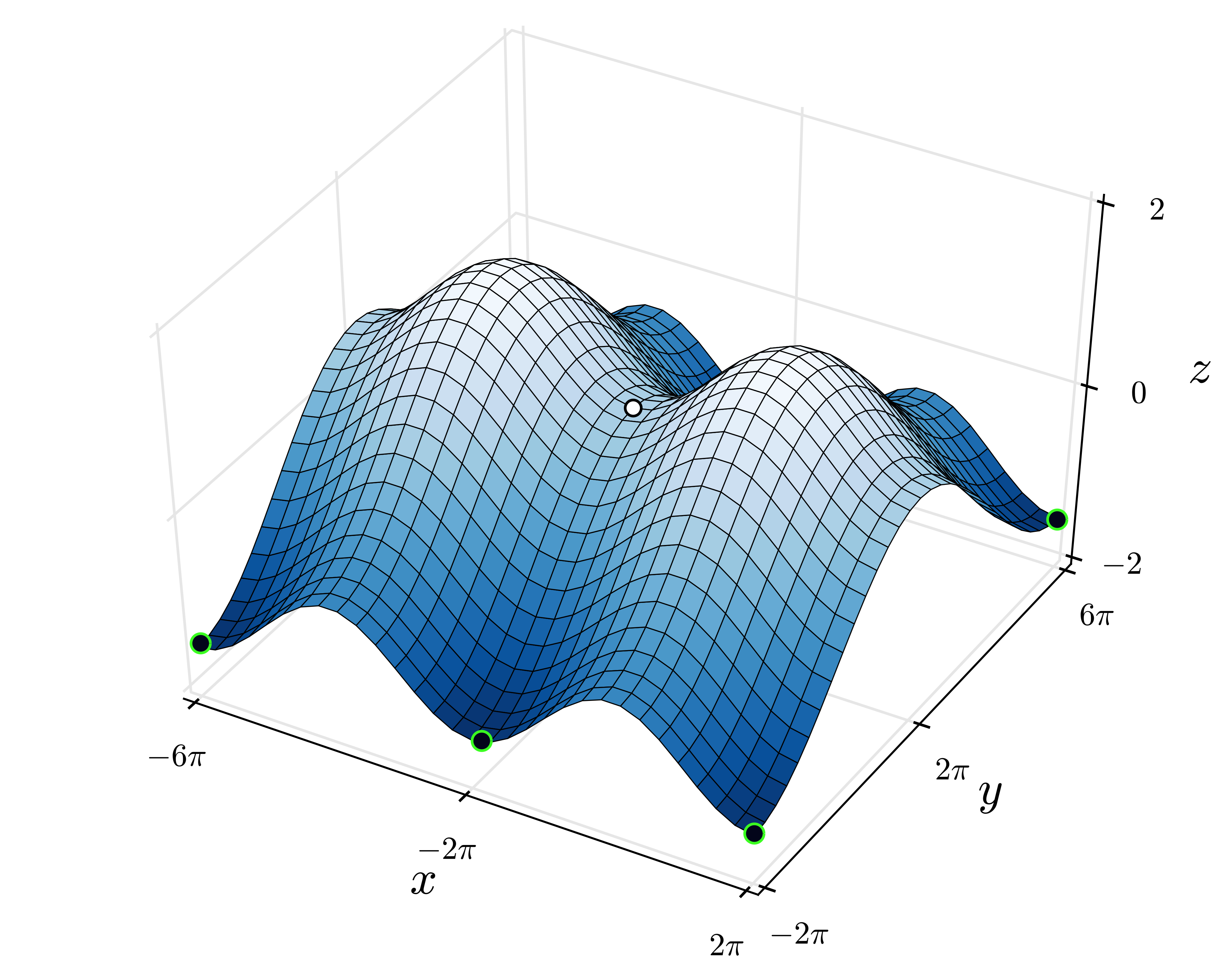
Figure 5: Illustration of saddle points and a functional landscape where local minima are global minima; the white dot in the middle, and black dots at the corners are a saddle point, and local/global minima, respectively.

II.6.3 Symmetry-stability analysis through Hessian

To investigate the preceding hypothesis, we analyze the stability of the circuit symmetries. The stability analysis is performed by analyzing the Hessian of DNNs, as introduced in the following.

In physics, as order parameters are associated with the first order symmetric excitation of units in response to excitation, the stability of order is characterized by the second order effect of such excitation (e.g., magnetic susceptibility). Thus, the stability of symmetries is characterized through Hessian of the free energy—a review of Hessian analysis of phases in physics could be found in supp. D E. Hessian of a potential function informs us of the local geometry of the risk landscape: when the gradient at a state is zero vector, negative eigenvalues of the Hessian inform that at the current state, descent directions in the parameter space exist to further reduce the potential; otherwise, the current state is a local minimum. A illustration of local geometry of risk landscape is given in fig. 5. Thus, to study the stability of the coarse-grained effect of circuit symmetry, we need to study the coarse-grained effect of circuit symmetries on the Hessian of the variational free energy.

To further clarify, to appreciate the study of stability of symmetries under the context of DNNs, note that the nonzero of plasticity order parameter observed in section II.5 results from symmetric statistical fluctuations of basis circuits that are only weakly dependent on the other basis circuits, however, these are experimental results obtained by sampling the order parameters. Theoretically, despite the speculative weak dependence, it could still be zero probabilistically. More concretely, geometrically, recall that the self-organizing process is a gradient descent process on the risk (variational free energy) landscape—recall that in section II.3, we have explained that risk is also variational free energy. Thus, the local curvature of the risk landscape could be irregular, and probabilistically, the order parameter could still be zero and the system could still stick trapped at nonzero local minima.

II.6.4 Coarse-grained effect of circuit symmetries on Hessian entries

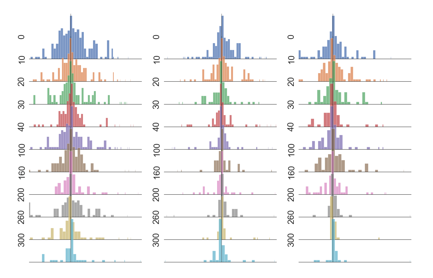
(a)

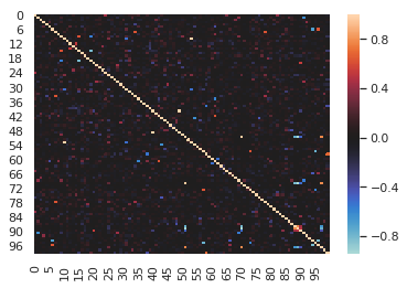
(b)

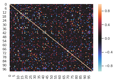
(c)

Figure 6: Adaptive symmetry of Hessian entries throughout training, and sparse correlation among Hessian entries at the beginning and the ending of DNN training. (a) Hessian entries are perturbation of neuron assemblies of order two. They are also experimentally found to be approximately self-similar as the gradients do. More specifically, the figure shows the probability density distributions of three randomly sampled Hessian entries, from left to right, throughout training respectively. The numbers on the left are the epoch numbers during training where the entry is sampled. Though we only show three entries for demonstration, we have sampled many more entries and the behaviors are similar. Both the x-axis and the y-axis are in the logarithmic scale. The Hessian entries are normalized by their standard deviations, respectively; that is, the normalization is entry-wise: each Hessian entry is divided/normalized by its standard deviation to compare it with the fluctuations of this entry. The probability distribution of Hessian entries are computed with bootstrap methods, of which the details is collected in supp. I A. The basic idea is to repeatedly sample the quantities of interest, and so long as the quantities under sampling are of limited variations, the sample would serve as an estimation of the quantities. In retrospect, circuit symmetries have enabled us to observe stable behaviors by such a sampling method, which is similar to the phenomenon that translation symmetry enables stable experimental observations for repeated experiments performed at different geo-locations. (b) (c) are the correlation coefficient (CC) matrices of Hessian entries at the beginning and the end of training, respectively. The diagonal line is the variance, which is 1 as the result of normalization by standard deviation. We uniformly randomly subsample a $100\times 100$ CC submatrix from a large CC matrix—the small size $100$ is chosen to let the readers be able to distinguish the pixels in the images. The CC matrix is obtained from the bootstrap sample of Hessian entries noted in fig. 6a.

The coarse-grained effect of (partial broken) circuit symmetries results in the statistically stable assembly-level adaptive symmetry (cf. the symmetric distribution of gradients in section II.5, which are also neurons assemblies), which we discuss next.

First, as in the case of the order parameter where the gradients are neuron assemblies that coarse-grains over the perturbation of basis circuits of order one, the Hessian are neuron assemblies that coarse-grains over the perturbation of basis circuits of order two. More specifically, the second-order perturbation of risk in the circuit form is given as

$$\delta\bm{\theta}^{T}\bm{H}\delta\bm{\theta}= \sum_{l=1}^{L}\sum_{l^{\prime}=1}^{L}\sum_{i_{l-1}=1}^{n_{l-1}}\sum_{i_{l}=1}^{n_{l}}\sum_{i_{l^{\prime}-1}=1}^{n_{l^{\prime}-1}}\sum_{i_{l^{\prime}}=1}^{n_{l^{\prime}}}$$ (18)

$$\sum_{\bm{i}\in I^{\setminus\{l-1,l,l^{\prime}-1,l^{\prime}\}}_{i_{l-1}i_{l}i_{l^{\prime}-1}i_{l^{\prime}}}}\mathbb{E}[\Omega^{\overline{l}_{\setminus\{l,l^{\prime}\}}}_{\bm{i}}]\delta w^{l}_{i_{l-1}i_{l}}\delta w^{l^{\prime}}_{i_{l^{\prime}-1}i_{l}^{\prime}},$$

where $\bm{H}$ denotes the Hessian matrix of risk, and $\delta\bm{\theta}^{T}$ is vectorized weight perturbations,

$$\Omega^{\overline{l}_{\setminus\{l,l^{\prime}\}}}_{\bm{i}}:=\Psi^{1\sim l-1}_{\bm{i}_{:l}}\Psi^{l+1\sim l^{\prime}-1}_{\bm{i}_{l:l^{\prime}}}\Psi^{l^{\prime}+1\sim L}_{\bm{i}_{l^{\prime}:}},$$ (19)

and $I^{\setminus\{l-1,l,l^{\prime}-1,l^{\prime}\}}_{i_{l-1}i_{l}i_{l^{\prime}-1}i_{l^{\prime}}}$ denotes

$$\overrightarrow{\otimes}_{\{p\in\overline{l}|p<l-1\}}[n_{p}]\otimes\{i_{l-1}\}\otimes\{i_{l}\}\overrightarrow{\otimes}_{\{p\in\overline{l}|l<p<l^{\prime}-1\}}[n_{p}]$$

$$\otimes\{i_{l^{\prime}-1}\}\otimes\{i_{l^{\prime}}\}\overrightarrow{\otimes}_{\{p\in\overline{l}|p>l\}}[n_{p}].$$

Although the equations look complicated, eq. 18 is simply the coarse-graining of the second-order perturbation of basic circuit $\Psi^{\overline{l}}_{\bm{i}}$ induced by the perturbations of circuit weights at layer $l,l^{\prime}$, i.e., $\delta w^{l}_{i_{l-1}i_{l}}\delta w^{l^{\prime}}_{i_{l^{\prime}-1}i_{l}^{\prime}}$—it is also explained with an illustration previously in fig. 2.

Second, as a result of heterogeneous circuit symmetries, even if a substantial subset of the circuits are of broken circuit symmetries, the coarse-grained behaviors of circuits could still be close to in the case where all circuit symmetries are intact. To illustrate the phenomenon, we present the upper bounds on the moments of assemblies as follows. Let $\{\delta^{k}\Psi^{1\sim L}_{\bm{i}}\}_{\bm{i}\in\mathcal{B}_{k}}$ be perturbation of basis circuits, and $\mathcal{B}_{0},\mathcal{B}_{1},\mathcal{B}_{2}$ denotes $I,I^{\setminus\{l-1,l\}}_{i_{l-1}i_{l}},I^{\setminus\{l-1,l,l^{\prime}-1,l^{\prime}\}}_{i_{l-1}i_{l}i_{l^{\prime}-1}i_{l^{\prime}}}$, respectively. Suppose that $\forall n_{l}=n\in\mathbb{N}^{+}$, and there exists $\mu>0,\mu\in\mathbb{R}$, such that $\sqrt{n}^{1-\mu}$ weights are of broken weight symmetry at each layer, then we have

$$\mathbb{E}[\sum_{\bm{i}\in\mathcal{B}_{k}}\delta^{k}\Psi^{1\sim L}_{\bm{i}}]\leq O\left((\frac{c^{2}}{2})^{L}+\frac{1}{\sqrt{n}^{L\mu}}c^{L}\right),$$ (20)

$$\mathbb{E}[(\sum_{\bm{i}\in\mathcal{B}_{k}}\delta^{k}\Psi^{1\sim L}_{\bm{i}})^{2}]\leq O\left(c^{2L}+(\frac{c^{2}}{2})^{2L}+\frac{1}{\sqrt{n}^{2L\mu}}c^{2L}\right),$$

where $\delta^{k}\Psi^{1\sim L}_{\bm{i}}$ is a shorthand notation for $\Psi^{1\sim L}_{\bm{i}},k=0$, $\Omega^{\overline{l}_{\setminus\{l\}}}_{\bm{i}},k=1$, $\Omega^{\overline{l}_{\setminus\{l,l^{\prime}\}}}_{\bm{i}},k=2;$ the derivation is in the supp. B E 6—note that the assembly ($k=2$) here computes a Hessian entry while eq. 18 further coarse-grains all Hessian entries. Notice that for a hierarchically large DNN, $\sqrt{n}^{L}$ and $2^{L}$ are both very large value, and thus the means are close to zero, and the squared norm of assemblies are close to $c$ (which is close to $1$ through initialization—this is a carefully maintained edge-of-chaos condition, and interested readers could find more discussion in supp. C B). The decay of mean is a special case of higher order moments where weights of odd power exists: when calculating the odd moments of a basis circuit $H^{L}_{i_{L}}W^{l}_{i_{l-1}i_{l}}\Psi^{1\sim L-1}_{i_{1}\ldots i_{L-1}}$, the integration against $W^{L}_{i_{l-1}i_{l}}$ over $[-\infty,0]$ and $[0,+\infty]$ would almost cancel out, and only leaves a residual because weights and neuronal gates are sparsely and weakly correlated; further notice that odd powered weights at each layer would induce a decay, and thus an exponential decay against depth is induced. Further notice that for higher moments, the majority of cross-moments among basis circuits (e.g., $\Psi^{1\sim L}_{\bm{i}}\Psi^{1\sim L}_{\bm{j}}\Psi^{1\sim L}_{\bm{k}}$) have odd power weights. Therefore, we might speculate a close-to-zero mean and sparse correlation among Hessian entries.

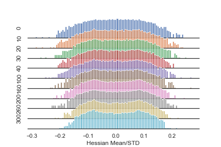
(a)

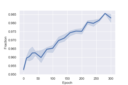
(b)

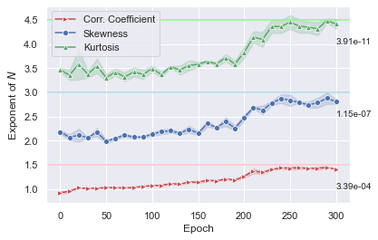
(c)

Figure 7: Experimental support for the assembly-symmetry assumption. (a) The probability density distribution of means of Hessian entries throughout training. The entries are also obtained by the bootstrap method summarized in fig. 6a, and the means are normalized by standard deviations of Hessian means to weep out the influence of magnitude throughout training and reveal the consistent symmetry. (b) The fraction of standard-deviation-normalized means that are less than 0.15 throughout training. The transparent region is the standard deviations of the fractions estimated through the bootstrap methods summarized in the caption of fig. 7a—because the fractions are estimated through the bootstrap method, the standard deviations are plotted to show that the estimated fractions are stable estimations. (c) Experimental support for the assembly-diversity and assembly-diversity assumption. The average order parameter, i.e., coupling set size, (over all Hessian entries) is estimated through the average non-zero statistics (of all Hessian entreis), i.e., correlation coefficients, skewness, and excess kurtosis, in term of the exponent of Hessian dimension $N$ during training, shown as curves in the figure. The non-zero correlation coefficients of each entry is equivalent to its coupling set size: the details on the relationship between the number and coupling set sizes is given in supp. B G 7. The transparent regions are standard deviations from the bootstrap samples in the experiments. The light color straight lines and the annotated numbers in the rightmost indicate the ratio between the non-zero number and the overall number of the statistics (both zero and non-zero). The numbers are estimated from bootstrap methods described in supp. I B.

Indeed, we experimentally compute mean and correlations among Hessian entries, and found that the Hessian entries fluctuate around zero and are of sparse correlations among one another, which could be appreciated as adaptive-symmetry and diversity of neuron assemblies, as explained in the following.

1. The adaptive symmetry of biotic systems has been introduce in section II.4, and the adaptive symmetry of Hessian entries manifest as the phenomenon that the Hessian entries fluctuate around zero such that random fluctuations could be converted into system-wide asymmetric behaviors in response to feedback signals—that is, the system poses to adapt symmetrically.

2. And in biotic systems, diversity begets complexity [137]: biotic systems evolve from low fitness states—relatively speaking—through a series of adjacent states to high fitness states on the frustrated fitness landscape by increasing diversity of the system. And such diversity exists in neuron assemblies as well. At initialization, DNNs are in a disordered state where the weights among neurons are independently randomly sampled; that is, a set of neurons with a diversity of possible coupling. Accordingly, different signals would activate a different set of neurons in the network randomly. During risk minimization by gradient descent, the weights are adjusted by the gradient computed by back-propagation until convergence. For a hierarchical large network, the number of possible paths (i.e., basis circuits) among neurons grow exponentially with depth, and thus at each weight update, the information only flows within a subset of neurons that are small compared with the overall number of possible circuits. Correspondingly, the after the training, though for a given signal, circuits are formed to classify it, for different signals, neurons still are activated largely uncorrelatedly and thus seemingly randomly. And thus the diversity of weights is a stable characteristic, and induces a mixture of order and disorder through training. This mixture manifests at the assembly level as functional behaviors (e.g., the prediction of a DNN) of, and the sparse correlation among assemblies: the seemingly random activation of assemblies would result in low correlation among them. And thus the Hessian entries are of sparse correlation among one another.

Experimentally, from fig. 6a, we could see that the Hessian entries are distributed approximately symmetrically against $y$-axis—a self-similar adaptive symmetry between Hessian entries (i.e., neuron assemblies of order two) and the microscopic basis circuits, as that of the gradient (i.e., neuron assemblies of order one), and thus fluctuate around zero throughout training. From fig. 6b and 6c, we could see that the correlations among Hessian entries are rather sparse, and the correlations increases after training, presumably because the circuit symmetries are broken to encode information in the dataset, and thus the statistical dependence among Hessian entries increase. Figure 7 shows that throughout the training, the means concentrate on zero in the sense that most of the means do not fluctuate further than $0.15$ standard deviation from zero, which is clearly a concentration of measure on zero, more quantitatively, from fig. 7b we can see that throughout training, the fraction of the means that are less than $0.15$ is at least $95\%$, and as the training progresses, the percentage gradually increases up to around $98\%$. We further quantitatively estimate the average number of Hessian entries each individual Hessian entries (referred as coupling set size) are correlated with by computing the averages (over all Hessian entries) of the number of non-zero covariances, skewnesses, and excess kurtoses respectively throughout training, and the result is given in fig. 7c. As shown by the light red line in fig. 7c at the end of the training, for a given Hessian entry, of overall $8.68\cdot 10^{12}$ possible coefficients between it and the rest of the entries—the network contains $N=8.68\cdot 10^{12}$ number of parameters—it only correlates $3.39\cdot 10^{-4}$ of them. Thus, each Hessian entry has a very large absolute coupling set size and a very small relative coupling set size compared with all the possible entries; the former encodes dependency among data, and the latter shall enable adaptability.

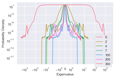
(a)

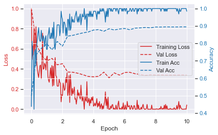
(b)

Figure 8: Plasticity phase, extended symmetry breaking and benign pathways of DNNs. Hessian eigenspectrum is also a neuron assembly, and under assumptions that characterize abundance of circuit symmetries, is theoretically (through a theorem that analyzes the statistical hierarchical many-body interaction among circuits) and experimentally found to be self-similar as the gradients do as well, as shown in fig. a. Such adaptive symmetry of eigenspectrum throughout training implies that despite the circuit symmetries that break to decrease the risk, the coarse-grained behaviors of the circuit symmetries are macroscopically (system-widely) stable, and according to the epistemology of physics, is a phase of the system, and is referred as the plasticity phase. The plasticity phase of DNNs is an extended adaptive-symmetries breaking process extended over time where circuit symmetries continually break to reduce informational perturbations and encode information from the environment. In the process, all stationary points are saddle points, and benign pathways exist such that by following gradients, zero risk could be reached, as shown in fig. b. To clarify, a subtlety exists in the problem setting (introduced in section I.1.3) of this work, and strictly speaking it is not that the eigenspectrum of Hessian is symmetric but a matrix in a decomposed form of Hessian. (a) Adaptive symmetry of Hessian eigenspectrum throughout DNN training. The numerically computed eigenspectrum of Hessian of the 12-layer VGGNet (cross entropy loss replaced by hinge loss) being trained on modified CIFAR10 datasets for binary classification. The numbers in the legends are epoch numbers in training. Note that the axes are in logarithmic scale. The eigenspectrum is computed with the Lanczos spectrum approximation algorithm [138, 139, 140] (details in supp. H). (b) The loss (empirical risk) and performance (accuracy) curves throughout DNN training. The loss measures the gradually decrease of the informational perturbations induced by examples in the training set, and the accuracy measures the emergence of functional specialization that does classification on the CIFAR dataset. Their change results from the breaking of circuit symmetries.

II.6.5 Plasticity phase, extended symmetry breaking, and benigh pathways of DNNs

We formulate those experimentally observed coarse-grained behaviors in hierarchically large DNNs as assumptions, which could be appreciated as conditions on coarse-grained behaviors in statistical physics referred as control parameters such as temperature, but are more heterogeneous because of the heterogeneity of circuits. And under these assumptions, further analysis of Hessian reveals a phase that is referred as the plasticity phase—thus, the parameters in the assumptions would be appreciated as preconditions on control parameters that identify a region of the parameter space that is a phase, and interested readers could find the discussion in the supplementary. Meanwhile, the phase is both a phase of a DNN, where the DNN could continually decreases risk, and an extended symmetry-breaking process, where the symmetries are continually being broken during the self-organizing process. As a result, benign pathways exist that lead to zero risk. We discuss these results next.

To begin with, we briefly contextualized the technique used in the analysis. The assumptions characterize a phenomenon of disorder at the assembly level, which is mathematically equivalent to the disorder at the field level in statistical physics. And it is not surprising that we could reuse the techniques developed there to analyze the disorder here. More specifically, sparsely correlated random matrices are being studied actively in the random matrix community, and in our setting—which is explained in section II.7, and could be roughly understood as the setting that DNNs do binary classification with the hinge loss—the Hessian belongs to a class of random matrices known as the Wigner-type matrix. The interests of Wigner-type matrices began with its ability in modeling the nuclei of heavy atoms, which is a disordered physical system that consists of a large number of interacting subatomic units (i.e. nucleons) [141, 142]. Though interaction exists among the subatomic units, the mathematical difficulty in characterizing random matrices with interaction/correlations is significant, and the early works in field, e.g., the Wigner matrix [141], ignored the correlation among units. We shall build on recent advances [53, 55, 56] that allow the correlation among matrix entries.

Under the preceding assumptions, we present a theorem that characterizes a concentration-of-measure phenomenon, and states that for a hierarchically large DNN, the eigenspectrum of its Hessian is symmetric w.r.t. $y$-axis throughout training; that is, the coarse-graining given in eq. 18 is self-similar to the circuit symmetry of basis circuits. More specifically, the size of a DNN is characterized by the number of parameters, which depends on both width and depth. For example, let $n_{l}$ denote the width of a DNN (of depth $L$) at layer $l$, then, it has $N=\sum_{l=1}^{L}n_{l-1}n_{l}$, or $N=Ln_{0}^{2}$ (assuming $\forall l\in\mathbb{L},n_{l-1}=n_{l}=n_{0}$), number of parameters, which is a function of both depth and width. This hierarchical largeness has taken the mantle of overparameterization in the literature, and their relationship is further discussed with related works in supp. A D. Informally, we have

$$\forall\lambda\in\mathbb{R},\mu_{\bm{H}}(\lambda)\approx\mu_{\bm{H}}(-\lambda),$$

where $\mu_{\bm{H}}$ denotes the eigenspectrum (i.e., probability density distribution of eigenvalues) of $\bm{H}$—the formal version is a probability bound in a theorem given in supp. B H 5. The symmetry of eigenspectrum implies that despite the broken circuit symmetry in the self-organizing process, the order (i.e. the ability to decrease risk) is stable because stationary point where the gradients (order parameter) is zero could only be saddle points, and the risk decrease would not be trapped in local minima. Therefore, in the regimen where circuit symmetry dominates over broken circuit symmetry, the risk could be minimized until its lower bound is reached, and for a well designed loss function, its the lower bound is zero. In other words, zero risk could be reached by following gradients through the feedback-control loop of a DNN. Furthermore, a lower risk concentrates eigenvalues more towards zero.

Experimentally, the stability of symmetries can be seen from fig. 8a, which shows that the eigenspectrum of the DNN’s Hessian is symmetrically distributed against $y$-axis throughout training. Figure 8a also shows that the convergence of the eigenspectrum to zero as training progress. Meanwhile, the broken symmetries also macroscopically manifests as the decrease of risk as training progress. This can be seen in fig. 8b, where the empirical risk (i.e., loss) converges to zero and the training accuracy converges to $1$.

Plasticity phase.

Therefore, the conditions in the assumptions demarcate a region of the state/weight/parameter space, where an abundant reservoir of circuits with circuit symmetry exist (along with broken circuit symmetries that encode information of the dataset), and thus the order parameter is stably nonzero when information perturbations (novel examples) exist. And as discussed in section II.4, unlike physical systems, where the invariant are invariants of invariants, the invariant of DNNs is the invariant of variants. Thus, the region of state space where such stability of the coarse-grained effect of circuit symmetries exists as a phase of DNNs. We refer the phase as the plasticity phase.

Extended symmetry breaking.

Meanwhile, the phase is both a phase of a DNN, where the DNN could continually decreases risk, and an extended symmetry-breaking process, where the symmetry is continually being broken during the self-organizing process. Although the adaptive symmetries of assemblies hold throughout the training, a subset of the circuits in the network transit from a symmetric distribution to outputs that correspond to zero risk of examples. That is, the excited perturbations gradually converge to zero, because the informational patterns are encoded in the network by circuits with broken circuit symmetries. In the Hessian spectrum, this manifests as its gradual convergence to a zero function because the examples in the training set are mapped to zero risk, which has a zero Hessian matrix. And at the end of the training, zero risk is reached.

Benign pathways.

Consequently, in the plasticity phase, by following the gradient—that is, by continually absorbing to novel-example excitation by breaking the sufficient reservoir of circuit symmetries through the feedback-control loop introduced in section II.4—the system could decrease the risk without being trapped in local minima, and eventually reach zero risk given a (fixed) dataset. We refer the pathways found by gradients in this phase as benign pathways. And such pathways suggest an explanation on the optimization power of DNNs.

To clarify lastly, the plasticity phase does not automatically hold for any large DNNs processing any datasets. It is an intricate interaction between the neurons and the data, and the generalization to other network size, architectures or datasets should be studied case by case. It is desirable to derive efficient algorithms to ensure the assumptions are held online during DNN training, but this is considered future works.

II.7 Theoretical setting

Lastly, we give the detailed theoretical settings of this work.

1. We investigate multilayer/deep neural networks that are hierarchically large. As noted previously, we study complex systems, and for complex systems irregularities of individual units are only subdued into the ordered behaviors of the aggregated whole when the number of units are large enough. To let the concentration-of-measure phenomena discussed manifest, the networks need to be hierarchically large. This hierarchically largeness is roughly known as the overparameterized regimen in the literature, however, critical difference exists—as we use the term “hierarchical largeness” instead of overparameterization—and is discussed in supp. A D, where we discuss related works.

2. The study is specifically for DNNs with ReLU activation function, a feedforward architecture, and without biases in each layer’s parameters, which also include convolutional DNNs (CNNs) [143]—though the formalism is stated for multilayer preceptron, CNNs mathematically are MLPs with sparse connection and shared weights. As introduced in section II.2, ReLU is a form of degenerated Monte Carlo sampling. The formalism could generalize to some activation functions that are variants of ReLU, e.g., Swish [144] and skip-connection architecture like ResNet [145], but they are not pursued in this work and are considered future works. Meanwhile, this formalism does not apply for activation function like Sigmoid or Tanh: the circuit symmetries do not hold for Sigmoid or Tanh. This fact also corroborates with the fact that DNNs with ReLU are much easier to train than those activation functions. Some further discussion on activation function and circuit symmetries could be found in supp. A D 2, where we discuss empirical works that study the risk landscape of DNNs. In the experiments, no biases are used.

3. We study DNNs that do binary classification. As introduced previously, DNNs are studied by analyzing the feedback-control loop between the hierarchical circuits and coarse-grained variables. Theoretically, the coarse-grained variable could be any form, however, to investigate the principle underlying DNNs without unnecessary complications, we study DNNs that do binary classification. In this case, the coarse-grained variable is a single output neuron at the top layer that classifies macroscopic patterns composed by a large number of microscopic units, e.g., pixels. And the loss function composed with DNNs belongs to a class of loss functions whose representative is the hinge loss. The class of loss functions are formally characterized in supp. B C 8. And the class of functions do not include quadratic loss, or cross entropy loss. Such restriction was firstly studied in Choromanska et al. [146] (cf. supp. A D 4 for related-works discussion from the statistical-physics approach). This is a beachhead problem that is simple yet nontrivial: this setting is the first problem of two interdependent problems that make up the general setting. For interested readers, the problem decomposition is given in supp. G A 3, and furthermore, how the results in this work could potentially generalize to all kinds of loss functions is also given in supp. G A 2.

4. We do not made any assumptions on input data except that they are normalized to the order of magnitude $\Theta(1)$; or, putting it in another way, the theoretical results apply to practical data. To elaborate, the assumptions introduced in section II.6.4 characterize a certain interaction between neurons and data such that when processing the data, certain adaptive symmetries and diversity exist in the neuron assemblies. As discussed in section III, the assumptions could be understood as certain complexity-matching between the dataset and the network.

Overall, except for relatively the simple loss function, the setting is the setting that is widely used in practice.

III Discussion: complexity from adaptive-symmetries breaking

The results introduced from section II.1 to II.6 compose an iteration of scientific inquiry where falsifiable hypotheses are developed from a formalism of the phenomenon and then are experimentally validated. Yet, it leaves many problems not investigated. In supp. C, we shall venture into the creative side of scientific inquiry, and try to make sense of the this work in relation to science in general. We briefly remark the contents there in this section for interested readers.

In supp. C, we clarify understudied concepts in the extended symmetry-breaking process of DNNs, and point out the connection between adaptive-symmetries breaking and complexity. More specifically, the plasticity phase characterized in this work looks like a paradox: in the plasticity phase, a DNN both possesses the stability of coarse-grained circuit symmetries, and the continual breaking of microscopic circuit symmetries. The paradoxical behaviors of DNNs could be appreciated as the paradigmatic-shift behaviors of organized complex systems in the sense of Kuhn’s [33] paradigm shift in science. Particularly, DNNs belong to the class of systems that are known as organized complexity [1], and are referred as complex systems [2, 3, 4, 5, 6, 7]. And this superficially paradoxical behavior emerges from the increased potential complexity of the DNN system. Furthermore, the increase of potential complexity also requires qualitative generalization of certain foundational concepts in statistical physics, such that they could be applied to the DNN organized complex system. In supp. C, we expand on the discussion here. We first put DNNs in a spectrum of phenomenological models that characterize increasingly complex systems in nature, and it is from this complexity increase, that the paradoxical behaviors emerge. Then, we discuss the generalized (from physics) concepts of criticality and phase transition of DNNs. Lastly, we discuss the self-organization of DNNs from the perspective of complexity increase. We given the outline in the following.

Phenomenological models with increasing complexity: spin glasses and DNNs.

First, in supp. C A 1, we compare the training process of DNNs with the frustration process of spin glasses, and in supp. C A 2, point out that the paradox of breaking and stable symmetries could be appreciated by putting spin glasses and DNNs in a spectrum of models with increasing potential complexity: it is the vastly increased potential complexity—which we mean by a hierarchically large DNNs with abundance of reservoir of circuits with circuit symmetries—enables a diachronic “frustration” process where circuit symmetries continually break, and makes the self-organizing of DNNs both a symmetries-breaking process and a phase with stable symmetries.

Extended criticality.

Second, the study of symmetry breaking in this work might be confusing without mentioning the criticality, which is a concept associated with symmetry breaking in physics. In supp. C B, we clarify the concept of criticality in DNNs. In physics, symmetry breaking is associated with power-law criticality. However, as the self-organizing process extends from a frustration process to a diachronic learning process, the criticality of DNNs is also spatially and temporally extended. More specifically, the concept of criticality needs to be reconceptualized as extended criticality [38] in theoretical biology, which is introduced in supp. C B 1 and states that the criticality of biotic systems lies in an extended region of the state space instead of singular points (as in the physical systems). In supp. C B 2 the self-organizing of DNNs is characterized as a process where the system computes at extended criticality to encode information and decrease uncertainty. The concept of extended criticality was developed further from the concept of edge of chaos [147, 42, 148], which under the context of biology refers to the phenomenon that the biotic systems are in a diachronic evolving process in regions of the state space that is between chaos and equilibrium. The concept that a DNN computes at edge of chaos is not novel, and existing works [149, 150, 151, 152] have interpreted the training of DNNs as such. Here, although the relationship between circuit-symmetry breaking and edge of chaos has not been discussed before, the discussion is mostly to clarify the criticality in the symmetry-breaking of DNNs. In supp. C B 3, we show that, mostly empirically, the a DNN self-organizes in the extended critical regimen during training.

Extended phase transition.

Third, as an extended symmetry-breaking process, theoretically, the reservoir of circuit symmetries could eventually be exhausted, therefore, in supp. C C, we shall discuss the self-organizing process from the perspective of extended phase transition. We have studied the region of the phase space where circuit symmetries coexist stably with broken circuit symmetries. As the symmetry-breaking is kept being broken—when more complex datasets are being processed—a DNN theoretically could run out of circuit symmetries. Therefore, we tentatively classify the self-organizing process of DNNs into two phases: in addition to the plasticity phase with stable circuit symmetries, the other phase contains a paucity of adaptive symmetries that could easily be unable to decrease the errors of novel examples, and is referred as the frustration phase—note that the frustration here does not mean the system is trapped in local minima that are not global minima, but simply be of nonzero risk. Two phases are quantitatively characterized by the plasticity order parameter and Hessian: in the plasticity phase, the order parameter is nonzero (when novel examples still exist) and the Hessian’s spectrum is symmetric, and in the frustration phase, the order parameter is zero and the Hessian is likely positive semidefinite. Compared with the phase space of statistical physics, where the trajectories can be visualized as a function of order parameter against scalar control parameters thanks to the homogeneous symmetries, the phase space of DNNs is a high-dimensional manifold embedded in the ambient state/weight space. We shall discuss a toy case of the frustration phase in supp. C C 1 and remark the phase transition between the two phases in supp. C C 2, mostly to clarify that the extended symmetry-breaking should also be understood as an extended phase transition.

Complexity from adaptive-symmetries breaking.

Lastly, in supp. C D, we discuss that symmetry breaking and complexity is like a duality: the accumulation of a large number of broken adaptive symmetries manifest as the complex behaviors of a system. Therefore, we point out a shift of perspective where the self-organizing of DNNs could be studied from the perspective of breaking symmetries to that of increasing complexity. More specifically, in this work, we give a characterization of the risk minimization of DNNs as a process where the system self-organizes to minimize uncertainty by breaking a reservoir of adaptive-symmetries in the feedback-control loop between it and the environment where it is embodied. In doing so, we identify a plasticity phase of DNNs that suggests an explanation of the optimization power of DNNs. However, symmetry-breaking emphasizes the physical perspective, and DNNs’ self-organizing is also a computing process, where information about the environment is gradually encoded into the circuits. And this computing perspective could be qualitatively described as increasing complexity, referring the increasing complex patterns recognizable by DNNs. Therefore, we summarize the process as complexity from adaptive symmetries as follows.

DNNs are able to increase the potential complexity of the system plastically, and when the potential complexity of a system is larger than the complexity of a dataset, a DNN could absorb informational perturbations from the environment and self-organize into a functional structure that reaches a goal with zero training errors measured by a ncertain surrogate risk.

References

- Weaver [1948] W. Weaver, Science and Complexity, American Scientist 36, 536 (1948).
- Simon [1962] H. A. Simon, The Architecture of Complexity, Proceedings of the American Philosophical Society 106, 467 (1962).
- Anderson [1972] P. W. Anderson, More Is Different, Science 177, 393 (1972).
- Mitchell [2009] M. Mitchell, Complexity: A Guided Tour (Oxford University Press, Inc., USA, 2009).
- Erdi [2007] P. Erdi, Complexity Explained, Springer complexity (Springer Berlin Heidelberg, 2007).
- Nicolis and Nicolis [2012] G. Nicolis and C. Nicolis, Foundations of Complex Systems: Emergence, Information and Prediction, 2nd ed. (World Scientific Publishing Co., Inc., River Edge, NJ, USA, 2012).
- Thurner et al. [2018] S. Thurner, R. Hanel, and P. Klimek, Introduction to the Theory of Complex Systems (Oxford University Press, 2018).
- Rosenblueth et al. [1943] A. Rosenblueth, N. Wiener, and J. Bigelow, Behavior , Purpose and Teleology, Philosophy of Science 10, 18 (1943).
- Keller [2009] E. F. Keller, Organisms, machines, and thunderstorms: A history of self-organization, part two. Complexity, emergence, and stable attractors, Historical Studies in the Natural Sciences 39, 1 (2009).
- LeCun et al. [2015] Y. LeCun, Y. Bengio, and G. Hinton, Deep learning, Nature 521, 436 (2015).
- Krizhevsky et al. [2012] A. Krizhevsky, I. Sutskever, and G. E. Hinton, ImageNet Classification with Deep Convolutional Neural Networks, in NIPS (2012).
- He et al. [2015] K. He, X. Zhang, S. Ren, and J. Sun, Delving Deep into Rectifiers: Surpassing Human-Level Performance on ImageNet Classification, in ICCV (2015) arXiv:1502.01852 .
- Radford and Salimans [2018] A. Radford and T. Salimans, Improving Language Understanding by Generative Pre-Training, Tech. Rep. (OpenAI, 2018).
- Rolnick et al. [2019] D. Rolnick, P. L. Donti, L. H. Kaack, K. Kochanski, A. Lacoste, K. Sankaran, A. S. Ross, N. Milojevic-Dupont, N. Jaques, A. Waldman-Brown, A. Luccioni, T. Maharaj, E. D. Sherwin, S. K. Mukkavilli, K. P. Kording, C. Gomes, A. Y. Ng, D. Hassabis, J. C. Platt, F. Creutzig, J. Chayes, and Y. Bengio, Tackling Climate Change with Machine Learning, Tech. Rep. (Climate Change AI, 2019) arXiv:1906.05433 .
- Senior et al. [2020] A. W. Senior, R. Evans, J. Jumper, J. Kirkpatrick, L. Sifre, T. Green, C. Qin, A. Žídek, A. W. Nelson, A. Bridgland, H. Penedones, S. Petersen, K. Simonyan, S. Crossan, P. Kohli, D. T. Jones, D. Silver, K. Kavukcuoglu, and D. Hassabis, Improved protein structure prediction using potentials from deep learning, Nature 577, 706 (2020).
- Oxford Economics [2019] Oxford Economics, How robots change the world, Economic Outlook 43, 5 (2019).
- Wikipedia [2020] Wikipedia, Deepfake (2020).
- Plebe and Grasso [2019] A. Plebe and G. Grasso, The Unbearable Shallow Understanding of Deep Learning, Minds and Machines 29, 515 (2019).
- Glorot and Bengio [2010] X. Glorot and Y. Bengio, Understanding the difficulty of training deep feedforward neural networks, in AISTATS (2010).
- Dauphin et al. [2014] Y. Dauphin, R. Pascanu, C. Gulcehre, K. Cho, S. Ganguli, and Y. Bengio, Identifying and attacking the saddle point problem in high-dimensional non-convex optimization, in NIPS (2014) arXiv:1406.2572 .
- Baity-Jesi et al. [2018] M. Baity-Jesi, L. Sagun, M. Geiger, S. Spigler, G. B. Arous, C. Cammarota, Y. LeCun, M. Wyart, and G. Biroli, Comparing Dynamics: Deep Neural Networks versus Glassy Systems, in ICML (2018) pp. 324–333, arXiv:1803.06969 .
- Oquab et al. [2014] M. Oquab, L. Bottou, I. Laptev, and J. Sivic, Learning and Transferring Mid-Level Image Representations using Convolutional Neural Networks, in CVPR (2014) pp. 1717–1724.
- Zhang et al. [2016] C. Zhang, S. Bengio, M. Hardt, B. Recht, and O. Vinyals, Understanding deep learning requires rethinking generalization, in ICLR (2016) arXiv:1611.03530 .
- Lipton [2018] Z. C. Lipton, The Mythos of Model Interpretability, Queue 16, 31 (2018).
- Barredo Arrieta et al. [2020] A. Barredo Arrieta, N. Díaz-Rodríguez, J. Del Ser, A. Bennetot, S. Tabik, A. Barbado, S. Garcia, S. Gil-Lopez, D. Molina, R. Benjamins, R. Chatila, and F. Herrera, Explainable Explainable Artificial Intelligence (XAI): Concepts, taxonomies, opportunities and challenges toward responsible AI, Information Fusion 58, 82 (2020).
- Ovadia et al. [2019] Y. Ovadia, E. Fertig, J. Ren, Z. Nado, D. Sculley, S. Nowozin, J. V. Dillon, B. Lakshminarayanan, and J. Snoek, Can You Trust Your Model’s Uncertainty? Evaluating Predictive Uncertainty Under Dataset Shift, in NeurIPS (2019) arXiv:1906.02530 .
- Abdar et al. [2021] M. Abdar, F. Pourpanah, S. Hussain, D. Rezazadegan, L. Liu, M. Ghavamzadeh, P. Fieguth, X. Cao, A. Khosravi, U. R. Acharya, V. Makarenkov, and S. Nahavandi, A review of uncertainty quantification in deep learning: Techniques, applications and challenges, Information Fusion 76, 243 (2021).
- Szegedy et al. [2014] C. Szegedy, W. Zaremba, and I. Sutskever, Intriguing properties of neural networks, in ICLR (2014) arXiv:1312.6199v4 .
- Goodfellow et al. [2018] I. Goodfellow, P. McDaniel, and N. Papernot, Making machine learning robust against adversarial inputs, Communications of the ACM 61, 56 (2018).
- Jenkins et al. [2020] O. C. Jenkins, D. Lopresti, and M. Mitchell, Next Wave Artificial Intelligence: Robust, Explainable, Adaptable, Ethical, and Accountable, Tech. Rep. (Computing Community Consortium, 2020) arXiv:2012.06058 .
- Carleo et al. [2019] G. Carleo, I. Cirac, K. Cranmer, L. Daudet, M. Schuld, N. Tishby, L. Vogt-Maranto, and L. Zdeborová, Machine learning and the physical sciences, Reviews of Modern Physics 91, 45002 (2019).
- Zdeborová [2020] L. Zdeborová, Understanding deep learning is also a job for physicists, Nature Physics 16, 602 (2020).
- Kuhn [1970] T. S. Kuhn, The Structure of Scientific Revolutions (University of Chicago Press, Chicago, 1970).
- Laughlin and Pines [2000] R. B. Laughlin and D. Pines, The theory of everything, PNAS 97, 28 (2000).
- Sethna [2006] J. P. Sethna, Statistical Mechanics: Entropy, Order Parameters and Complexity, first edition ed. (Oxford University Press, Great Clarendon Street, Oxford, 2006).
- Bailly and Longo [2011] F. Bailly and G. Longo, Mathematics and the Natural Sciences: The Physical Singularity of Life, Advances in computer science and engineering: Texts (Imperial College Press, 2011).
- Longo and Montévil [2011] G. Longo and M. Montévil, From physics to biology by extending criticality and symmetry breakings, Progress in Biophysics and Molecular Biology 106, 340 (2011).
- Longo and Montévil [2013] G. Longo and M. Montévil, Extended criticality, phase spaces and enablement in biology, Chaos, Solitons and Fractals 55, 64 (2013).
- Popper [1934] K. R. Popper, The Logic of Scientific Discovery (Hutchinson, London, 1934).
- Laughlin et al. [2000] R. B. Laughlin, D. Pines, J. Schmalian, B. P. Stojkovići, and P. Wolynes, The Middle Way, PNAS 97, 32 (2000).
- Wiener [1965] N. Wiener, Cybernetics, Second Edition: Or the Control and Communication in the Animal and the Machine (The MIT Press, 1965).
- Kauffman and Johnsen [1991] S. A. Kauffman and S. Johnsen, Coevolution to the edge of chaos: Coupled fitness landscapes, poised states, and coevolutionary avalanches, Journal of Theoretical Biology 149, 467 (1991).
- Davidson and Erwin [2006] E. H. Davidson and D. H. Erwin, Gene regulatory networks and the evolution of animal body plans, Science 311, 796 (2006).
- Davidson [2010] E. H. Davidson, Emerging properties of animal gene regulatory networks, Nature 468, 911 (2010).
- Li and Bowerman [2010] R. Li and B. Bowerman, Symmetry breaking in biology, Cold Spring Harbor perspectives in biology 2, 1 (2010).
- Krakauer [2011] D. C. Krakauer, Darwinian demons, evolutionary complexity, and information maximization, Chaos 21, 10.1063/1.3643064 (2011).
- Montévil et al. [2016] M. Montévil, M. Mossio, A. Pocheville, and G. Longo, Theoretical principles for biology: Variation, Progress in Biophysics and Molecular Biology 122, 36 (2016).
- Mossio et al. [2016] M. Mossio, M. Montévil, and G. Longo, Theoretical principles for biology: Organization, Progress in Biophysics and Molecular Biology 122, 24 (2016).
- Flack [2017] J. Flack, Life’s information hierarchy, in From Matter to Life: Information and Causality (Cambridge University Press, 2017) pp. 283–302.
- Wolf et al. [2018] Y. I. Wolf, M. I. Katsnelson, and E. V. Koonin, Physical foundations of biological complexity, Proceedings of the National Academy of Sciences of the United States of America 115, E8678 (2018).
- Ramstead et al. [2018] M. J. D. Ramstead, P. B. Badcock, and K. J. Friston, Answering Schrödinger’s question: A free-energy formulation, Physics of Life Reviews 24, 1 (2018).
- Jost [2021] J. Jost, Biology, geometry and information, Theory in Biosciences 10.1007/s12064-021-00351-9 (2021).
- Helton et al. [2007] J. W. Helton, R. R. Far, and R. Speicher, Operator-valued semicircular elements: Solving a quadratic matrix equation with positivity constraints, International Mathematics Research Notices 2007, 1 (2007).
- Wainwright and Jordan [2008] M. Wainwright and M. Jordan, Graphical Models, Exponential Families, and Variational Inference, Foundations and trends in machine learning (Now Publishers, 2008).
- Erdos et al. [2019] L. Erdos, T. Kruger, and D. Schroder, Random Matrices with Slow Correlation Decay, Forum of Mathematics, Sigma 7, doi:10.1017/fms.2019.2 (2019).
- Alt et al. [2020] J. Alt, L. Erdos, and T. Krüger, The Dyson equation with linear self-energy: spectral bands, edges and cusps, Documenta Mathematica 25, 421 (2020).
- Li [2021a] S. W. M. Li, Complexity from Adaptive-Symmetries Breaking: Global Minima in the Statistical Mechanics of Deep Neural Networks, Tech. Rep. (2021).
- McKay et al. [1982] S. R. McKay, A. N. Berker, and S. Kirkpatrick, Spin-Glass Behavior in Frustrated Ising Models with Chaotic Renormalization-Group Trajectories, Physical Review Letters 48, 767 (1982).
- Rosati [2001] F. Rosati, RENORMALIZATION GROUP FOR SPIN GLASSES, International Journal of Modern Physics A 16, 2111 (2001).
- Çaǧlar and Berker [2017] T. Çaǧlar and A. N. Berker, Phase transitions between different spin-glass phases and between different chaoses in quenched random chiral systems, Physical Review E 96, 10.1103/PhysRevE.96.032103 (2017).
- Longo and Montévil [2019] G. Longo and M. Montévil, Comparing Symmetries in Models and Simulations, in Springer Handbook of Model-Based Science (2019) pp. 843–856.
- Laughlin [2014] R. B. Laughlin, A Perspective : Robert B Laughlin, Physical Biology 11, 053003 (2014).
- Seoane and Solé [2018] L. F. Seoane and R. V. Solé, Information theory, predictability and the emergence of complex life, Royal Society Open Science 5, 10.1098/rsos.172221 (2018).
- Krakauer et al. [2020] D. Krakauer, N. Bertschinger, E. Olbrich, J. C. Flack, and N. Ay, The information theory of individuality, Theory in Biosciences 10.1007/s12064-020-00313-7 (2020).
- Bravi and Longo [2015] B. Bravi and G. Longo, The unconventionality of nature: Biology, from noise to functional randomness, in Lecture Notes in Computer Science (LNCS), Vol. 9252 (2015) pp. 3–34.
- Mehta and Schwab [2014] P. Mehta and D. J. Schwab, An exact mapping between the Variational Renormalization Group and Deep Learning, Tech. Rep. (2014) arXiv:1410.3831 .
- Lin and Tegmark [2017] H. W. Lin and M. Tegmark, Why does deep and cheap learning work so well?, Journal of Statistical Physics 168, 1223 (2017).
- Flack et al. [2012] J. C. Flack, D. Erwin, T. Elliot, and D. C. Krakauer, 2 Timescales , Symmetry , and Uncertainty Reduction in the Origins of Hierarchy in Biological Systems, in Cooperation and Its Evolution (2012) pp. 45–74.
- Levin et al. [1997] S. A. Levin, B. Grenfell, A. Hastings, and A. S. Perelson, Mathematical and computational challenges in population biology and ecosystems science, Science 275, 334 (1997).
- Krakauer et al. [2011] D. C. Krakauer, J. P. Collins, D. Erwin, J. C. Flack, W. Fontana, M. D. Laubichler, S. J. Prohaska, G. B. West, and P. F. Stadler, The challenges and scope of theoretical biology, Journal of Theoretical Biology 276, 269 (2011).
- Heylighen and Joslyn [2001] F. Heylighen and C. Joslyn, 04. Cybernetics and second order cybernetics, in Encyclopedia of Physical Science and Technology, Vol. 4 (Academic Press, New York, 2001) pp. 155–169.
- Gorban and Tyukin [2018] A. N. Gorban and I. Y. Tyukin, Blessing of dimensionality: Mathematical foundations of the statistical physics of data, Philosophical Transactions of the Royal Society A: Mathematical, Physical and Engineering Sciences 376, 10.1098/rsta.2017.0237 (2018).
- Li [2021b] S. W. M. Li, See Supplemental Material in auxillary files on arxiv., Tech. Rep. (2021).
- Robinson [2018] A. Robinson, Did Einstein really say that?, Nature 557, 30 (2018).
- Simonyan and Zisserman [2015] K. Simonyan and A. Zisserman, Very Deep Convolutional Networks for Large-Scale Image Recognition, in ICLR (2015) arXiv:1409.1556 .
- Cohen et al. [2021] O. Cohen, O. Malka, and Z. Ringel, Learning curves for deep neural networks: A gaussian field theory perspective, Physical Review Research 3, 23034 (2021).
- Uexküll [1992] J. V. O. N. Uexküll, A stroll through the worlds of animals and men : A picture book of invisible worlds *, Semiotica 89, 319 (1992).
- Sigmund and Hofstadter [2017] K. Sigmund and D. Hofstadter, Exact Thinking in Demented Times: The Vienna Circle and the Epic Quest for the Foundations of Science (Basic Books, 2017).
- Jaynes [1967] E. T. Jaynes, Foundations of Probability Theory and Statistical Mechanics, in Delaware Seminar in the Foundations of Physics (Springer, Berlin, Heidelberg, 1967) pp. 229–255.
- Eguchi et al. [2018] A. Eguchi, J. B. Isbister, N. Ahmad, and S. Stringer, The emergence of polychronization and feature binding in a spiking neural network model of the primate ventral visual system, Psychological Review 125, 545 (2018).
- López-Rubio [2018] E. López-Rubio, Computational Functionalism for the Deep Learning Era, Minds and Machines 28, 667 (2018).
- Mahendran and Vedaldi [2015] A. Mahendran and A. Vedaldi, Understanding Deep Image Representations by Inverting Them, in CVPR (2015) arXiv:1412.0035 .
- Raghu et al. [2017] M. Raghu, J. Gilmer, J. Yosinski, and J. Sohl-Dickstein, SVCCA: Singular Vector Canonical Correlation Analysis for Deep Understanding and Improvement, in NIPS (2017) arXiv:1706.05806 .
- Bau et al. [2020] D. Bau, J. Y. Zhu, H. Strobelt, A. Lapedriza, B. Zhou, and A. Torralba, Understanding the role of individual units in a deep neural network, PNAS 117, 30071 (2020).
- Hoffmann et al. [2021] A. Hoffmann, C. Fanconi, R. Rade, and J. Kohler, This Looks Like That… Does it? Shortcomings of Latent Space Prototype Interpretability in Deep Networks, Tech. Rep. (2021) arXiv:2105.02968 .
- Castelvecchi [2016] D. Castelvecchi, The Blackbox of AI, Nature 538, 20 (2016).
- Krakauer et al. [2010] D. C. Krakauer, J. C. Flack, S. Dedeo, D. Farmer, and D. Rockmore, Intelligent data analysis of intelligent systems, Advances in Intelligent Data Analysis. Lecture Notes in Computer Science 6065, 8 (2010).
- Darwin [1936] C. Darwin, The origin of species, Everyman’s library (Dent, 1936).
- Koonin [2016] E. V. Koonin, The meaning of biological information, Philosophical Transactions of the Royal Society A: Mathematical, Physical and Engineering Sciences 374, 10.1098/rsta.2015.0065 (2016).
- Ay and Löhr [2015] N. Ay and W. Löhr, The Umwelt of an embodied agent—a measure-theoretic definition, Theory in Biosciences 134, 105 (2015).
- Mussardo [2020] G. Mussardo, Statistical Field Theory: An Introduction to Exactly Solved Models in Statistical Physics, Oxford Graduate Texts (Oxford University Press, 2020).
- Holland [2012] J. Holland, Signals and Boundaries: Building Blocks for Complex Adaptive Systems (MIT Press, 2012).
- Pearl [1988] J. Pearl, Probabilistic Reasoning in Intelligent Systems: Networks of Plausible Inference (Morgan Kaufmann Publishers Inc., San Francisco, CA, USA, 1988).
- Palacios et al. [2020] E. R. Palacios, A. Razi, T. Parr, M. Kirchhoff, and K. Friston, On Markov blankets and hierarchical self-organisation, Journal of Theoretical Biology 486, 10.1016/j.jtbi.2019.110089 (2020).
- Glorot et al. [2011] X. Glorot, A. Bordes, and Y. Bengio, Deep Sparse Rectifier Neural Networks, in AISTATS (2011).
- Bishop [2006] C. M. Bishop, Pattern Recognition and Machine Learning (Information Science and Statistics) (Springer-Verlag, Berlin, Heidelberg, 2006).
- Brush [1976] S. G. . Brush, Statistical Mechanics and the Philosophy of Science : Some Historical Notes, in Proceedings of the Biennial Meeting of the Philosophy of Science Association, Vol. 2 (1976) pp. 551–584.
- Ashby [1947] W. R. Ashby, Principles of the self-organizing dynamic system, Journal of General Psychology 37, 125 (1947).
- Nicolis and Prigogine [1977] G. Nicolis and I. Prigogine, Self-Organization in Nonequilibrium Systems: From Dissipative Structures to Order Through Fluctuations, A Wiley-Interscience publication (Wiley, 1977).
- von Foerster [2003] H. von Foerster, On Self-Organizing Systems and Their Environments, in Understanding Understanding (Springer, New York, 2003) Chap. 1, pp. 1–19.
- Heylighen [2002] F. Heylighen, The science of self-organization and adaptivity, The Encyclopedia of Life Support Systems 5, 253 (2002).
- Haken [2006] H. Haken, Information and Self-Organization: A Macroscopic Approach to Complex Systems (Springer Series in Synergetics) (Springer-Verlag, Berlin, Heidelberg, 2006).
- Camazine et al. [2003] S. Camazine, J. Deneubourg, N. Franks, J. Sneyd, E. Bonabeau, and G. Theraula, Self-organization in Biological Systems, Princeton Studies in Complexity (Princeton University Press, 2003).
- De Wolf and Holvoet [2005] T. De Wolf and T. Holvoet, Emergence versus self-organisation: Different concepts but promising when combined, Engineering Self-Organising Systems. ESOA 2004. Lecture Notes in Computer Science 3464, 1 (2005).
- Keller [2008] E. F. Keller, Organisms, machines, and thunderstorms: A history of self-organization, part one, Historical Studies in the Natural Sciences 38, 45 (2008).
- Spitzner and Polani [1998] A. Spitzner and D. Polani, Order parameters for self-organizing maps, in ICANN (1998) pp. 517–522.
- Gershenson and Heylighen [2003] C. Gershenson and F. Heylighen, When can we call a system self-organizing?, Lecture Notes in Artificial Intelligence (Subseries of Lecture Notes in Computer Science) 2801, 606 (2003).
- Shalizi et al. [2004] C. R. Shalizi, K. L. Shalizi, and R. Haslinger, Quantifying self-organization with optimal predictors, Physical Review Letters 93, 10.1103/PhysRevLett.93.118701 (2004).
- Polani [2008] D. Polani, Foundations and Formalizations of Self-organization, in Advances in Applied Self-organizing Systems (Springer, London, 2008) Chap. 2, pp. 19–37.
- Prokopenko [2009] M. Prokopenko, Guided self ‐ organization, HFSP Journal 3, 287 (2009).
- Rosas et al. [2018] F. Rosas, P. A. Mediano, M. Ugarte, and H. J. Jensen, An information-theoretic approach to self-organisation: Emergence of complex interdependencies in coupled dynamical systems, Entropy 20, 10.3390/e20100793 (2018).
- Gershenson [2020] C. Gershenson, Guiding the Self-Organization of Cyber-Physical Systems, Frontiers in Robotics and AI 7, 1 (2020).
- Friston et al. [2006] K. Friston, J. Kilner, and L. Harrison, A free energy principle for the brain, Journal of Physiology Paris 100, 70 (2006).
- Friston [2009] K. Friston, The free-energy principle: a rough guide to the brain?, Trends in Cognitive Sciences 13, 293 (2009).
- Friston [2010] K. Friston, The free-energy principle: A unified brain theory?, Nature Reviews Neuroscience 11, 127 (2010).
- Pezzulo et al. [2018] G. Pezzulo, F. Rigoli, and K. J. Friston, Hierarchical Active Inference: A Theory of Motivated Control, Trends in Cognitive Sciences 22, 294 (2018).
- Buckley et al. [2017] C. L. Buckley, C. S. Kim, S. McGregor, and A. K. Seth, The free energy principle for action and perception: A mathematical review, Journal of Mathematical Psychology 81, 55 (2017).
- Yufik and Friston [2016] Y. M. Yufik and K. Friston, Life and understanding: The origins of “understanding” in self-organizing nervous systems, Frontiers in Systems Neuroscience 10, 1 (2016).
- Yufik et al. [2017] Y. M. Yufik, B. Sengupta, and K. Friston, Editorial: Self-organization in the nervous system, Frontiers in Systems Neuroscience 11, 1 (2017).
- Prigogine [1978] I. Prigogine, Time, Structure, and Fluctuations, Science 201, 777 (1978).
- Vapnik [1998] V. N. Vapnik, Statistical Learning Theory (Wiley-Interscience, 1998).
- Kadanoff [2000] L. Kadanoff, Statistical Physics: Statics, Dynamics and Renormalization, Statistical Physics: Statics, Dynamics and Renormalization (World Scientific, 2000).
- Nishimori [2001] H. Nishimori, Statistical Physics of Spin Glasses and Information Processing: an Introduction (Oxford University Press, Oxford; New York, 2001).
- Gallavotti [2016] G. Gallavotti, Ergodicity: a historical perspective. Equilibrium and Nonequilibrium, European Physical Journal H 41, 181 (2016).
- Wadhawan [2011] V. Wadhawan, Latent, Manifest, and Broken Symmetry: A Bottom-up Approach to Symmetry, with Implications for Complex Networks (Createspace Independent Pub, 2011).
- Seung and Sompolinsky [1992] H. S. Seung and H. Sompolinsky, Statistical mechanics of learning from examples, Physical Review A 45, 6056 (1992).
- Watkin et al. [1993] T. L. Watkin, A. Rau, and M. Biehl, The statistical mechanics of learning a rule, Reviews of Modern Physics 65, 499 (1993).
- Haussler [1996] D. Haussler, Rigorous Learning Curve Bounds from Statistical Mechanics, Machine Learning 25, 195 (1996).
- Goldt et al. [2020] S. Goldt, M. Marc, F. Krzakala, and L. Zdeborová, Modeling the Influence of Data Structure on Learning in Neural Networks : The Hidden Manifold Model, Physics Review X 10, 1 (2020).
- Goldt et al. [2021] S. Goldt, B. Loureiro, G. Reeves, F. Krzakala, M. Mézard, and L. Zdeborová, The Gaussian equivalence of generative models for learning with shallow neural networks, in MSML (2021) pp. 1–46, arXiv:2006.14709v3 .
- Bartlett et al. [2017] P. Bartlett, D. J. Foster, and M. Telgarsky, Spectrally-normalized margin bounds for neural networks, in NIPS (2017) pp. 6240–6249, arXiv:1706.08498 .
- Neyshabur et al. [2019] B. Neyshabur, Z. Li, S. Bhojanapalli, Y. LeCun, and N. Srebro, The Role of Over-Parametrization in Generalization of Neural Networks, in ICLR (2019) arXiv:1805.12076 .
- Li et al. [2021] S. Li, K. Jia, Y. Wen, T. Liu, and D. Tao, Orthogonal Deep Neural Networks, TPAMI 43, 1352 (2021).
- Belkin et al. [2019] M. Belkin, D. Hsu, S. Ma, and S. Mandal, Reconciling modern machine-learning practice and the classical bias – variance trade-off, PNAS 116, 15849 (2019).
- Advani et al. [2020] M. S. Advani, A. M. Saxe, and H. Sompolinsky, High-dimensional dynamics of generalization error in neural networks, Neural Networks 132, 428 (2020).
- Kauffman and Kauffman [1993] S. Kauffman and M. Kauffman, The Origins of Order: Self-organization and Selection in Evolution (Oxford University Press, 1993).
- Page [2010] S. E. Page, Diversity and Complexity, 1st ed. (Princeton University Press, USA, 2010).
- Lin et al. [2016] L. Lin, Y. Saad, and C. Yang, Approximating spectral densities of large matrices, SIAM review 58, 34 (2016).
- Papyan [2018] V. Papyan, The Full Spectrum of Deep Net Hessians At Scale: Dynamics with Sample Size, Tech. Rep. (2018) arXiv:1811.07062 .
- Ghorbani et al. [2019a] B. Ghorbani, S. Krishnan, and Y. Xiao, An Investigation into Neural Net Optimization via Hessian Eigenvalue Density, in ICML (2019) pp. 2232–2241, arXiv:1901.10159 .
- Wigner [1957] E. P. Wigner, Statistical Properties of Real Symmetric Matrices with Many Dimensions, in Canadian Mathematical Congress Proceedings (1957).
- Guhr et al. [1998] T. Guhr, A. Müller-Groeling, and H. A. Weidenmüller, Random-matrix theories in quantum physics: Common concepts, Physics Report 299, 189 (1998).
- Lecun et al. [1998] Y. Lecun, L. Bottou, Y. Bengio, and P. Haffner, Gradient-based learning applied to document recognition, Proceedings of the IEEE 86, 2278 (1998).
- Ramachandran et al. [2018] P. Ramachandran, B. Zoph, and Q. V. Le, Searching for Activation Functions, in ICLR Workshop (2018) arXiv:1710.05941 .
- He et al. [2016a] K. He, X. Zhang, S. Ren, and J. Sun, Identity Mappings in Deep Residual Networks, in ECCV (2016) arXiv:1603.05027 .
- Choromanska et al. [2015a] A. Choromanska, M. Henaff, and M. Mathieu, The Loss Surfaces of Multilayer Networks, in AISTATS (2015) arXiv:1412.0233v3 .
- Packard [1988] N. Packard, Adaptation Toward the Edge of Chaos (University of Illinois at Urbana-Champaign, Center for Complex Systems Research, 1988).
- Gramß et al. [1998] T. Gramß, S. Bornholdt, M. Groß, M. Mitchell, T. Pellizzari, and M. Mitchell, Computation in Cellular Automata: A Selected Review, in Non-Standard Computation (Santafe Institute, 1998) pp. 95–140.
- Poole et al. [2016] B. Poole, S. Lahiri, M. Raghu, J. Sohl-Dickstein, and S. Ganguli, Exponential expressivity in deep neural networks through transient chaos, in NIPS (2016) arXiv:1606.05340 .
- Feng and Lai [2020] L. Feng and C. H. Lai, Optimal Machine Intelligence Near the Edge of Chaos, Tech. Rep. (2020) arXiv:1909.05176 .
- Zhang et al. [2020] G. Zhang, G. Li, W. Shen, and W. Zhang, The expressivity and training of deep neural networks: Toward the edge of chaos?, Neurocomputing 386, 8 (2020).
- Zhang et al. [2021] L. Zhang, L. Feng, K. Chen, and C. H. Lai, Edge of chaos as a guiding principle for modern neural network training, Tech. Rep. (2021) arXiv:2107.09437 .
- Gu et al. [2016] S. Gu, S. Levine, I. Sutskever, and A. Mnih, MuProp: Unbiased Backpropagation for Stochastic Neural Networks, in ICLR (2016) arXiv:1511.05176 .
- Welling [2014] M. Welling, Auto-Encoding Variational Bayes, in ICLR (2014) arXiv:1312.6114v10 .
- Gal and Ghahramani [2016] Y. Gal and Z. Ghahramani, Dropout as a Bayesian Approximation: Representing Model Uncertainty in Deep Learning, in ICML (2016) arXiv:1506.02142 .
- Wen et al. [2018] Y. Wen, P. Vicol, J. Ba, Dustin Tran, and Roger Grosse, Flipout: Efficient Pseudo-Independent Weight Perturbations on Mini-Batches, in ICLR (2018).
- Garriga-Alonso and Fortuin [2020] A. Garriga-Alonso and V. Fortuin, Exact Langevin Dynamics with Stochastic Gradients, in Symposium on Advances in Approximate Bayesian Inference (2020) pp. 1–10, arXiv:2102.01691 .
- Ou [2019] Z. Ou, A Review of Learning with Deep Generative Models from Perspective of Graphical Mod- eling, Tech. Rep. (2019) arXiv:arXiv:1808.01630v4 .
- Goan and Fookes [2020] E. Goan and C. Fookes, Bayesian Neural Networks: An Introduction and Survey, in Case Studies in Applied Bayesian Data Science (Springer Link, 2020) pp. 45–87, arXiv:2006.12024 .
- Masegosa et al. [2021] A. R. Masegosa, R. Cabañas, H. Langseth, and T. D. Nielsen, Probabilistic Models with Deep Neural Networks, Entropy 23 (2021).
- Hinton et al. [2006] G. E. Hinton, S. Osindero, and Y. W. Teh, A fast learning algorithm for deep belief nets., Neural computation 18, 1527 (2006).
- Salakhutdinov and Hinton [2009] R. Salakhutdinov and G. E. Hinton, Deep Boltzmann Machines, in AISTATS (2009) pp. 448–455, arXiv:1203.4416 .
- Memisevic and Hinton [2010] R. Memisevic and G. E. Hinton, Learning to represent spatial transformations with factored higher-order Boltzmann machines., Neural computation 22, 1473 (2010).
- Wenzel et al. [2020] F. Wenzel, K. Roth, B. S. Veeling, J. Świa̧tkowski, L. Tran, S. Mandt, J. Snoek, T. Salimans, R. Jenatton, and S. Nowozin, How good is the Bayes posterior in deep neural networks really?, in ICML (2020) pp. 10179–10190, arXiv:2002.02405 .
- Choi et al. [2020] Y. Choi, A. Vergari, and G. Van Den Broeck, Probabilistic Circuits : A Unifying Framework for Tractable Probabilistic Models, Tech. Rep. (2020).
- Vergari and Liu [2021] A. Vergari and A. Liu, A Compositional Atlas of Tractable Circuit Operations for Probabilistic Inference, in Workshop on Tractable Probabilistic Modeling (2021).
- Cammarata et al. [2020] N. Cammarata, S. Carter, G. Goh, C. Olah, M. Petrov, L. Schubert, C. Voss, B. Egan, and S. K. Lim, Thread: Circuits, Distill 10.23915/distill.00024 (2020), https://distill.pub/2020/circuits.
- Körner [1989] T. Körner, Fourier Analysis (Cambridge University Press, 1989).
- Mallat [2008] S. Mallat, A Wavelet Tour of Signal Processing: The Sparse Way, 3rd ed. (Academic Press, Inc., USA, 2008).
- Bruna and Mallat [2011] J. Bruna and S. Mallat, Classification with scattering operators, in CVPR (2011) pp. 1561–1566.
- Oyallon et al. [2014] E. Oyallon, S. Mallat, and L. Sifre, Generic Deep Networks with Wavelet Scattering, in ICLR Workshop (2014) arXiv:1312.5940 .
- Sifre and Mallat [2013] L. Sifre and S. Mallat, Rotation, Scaling and Deformation Invariant Scattering for Texture Discrimination, in CVPR (2013) pp. 1233–1240.
- Mallat [2012] S. Mallat, Group Invariant Scattering, Communications on Pure and Applied Mathematics LXV, 1331 (2012).
- Bruna and Mallat [2012] J. Bruna and S. Mallat, Invariant Scattering Convolution Networks, TPAMI 35, 1872 (2012).
- And and Mallat [2015] E. O. And and E. Mallat, Deep Roto-Translation Scattering for Object Classification, CVPR (2015).
- Mallat [2016] S. Mallat, Understanding deep convolutional networks., Philosophical transactions. Series A, Mathematical, physical, and engineering sciences 374, 10.1098/rsta.2015.0203 (2016).
- Jacobsen et al. [2017] J.-H. Jacobsen, E. Oyallon, S. Mallat, and A. W. M. Smeulders, Hierarchical Attribute CNNs, in ICML Workshop on Principled Approaches to Deep Learning (2017) arXiv:1703.04140 .
- Fukushima [1980] K. Fukushima, Neocognitron: A Self-organizing Neural Network Model for a Mechanism of Pattern Recognition Unaffected by Shift in Position, Biological Cybernetics 36, 193 (1980).
- Dieleman et al. [2016] S. Dieleman, J. De Fauw, and K. Kavukcuoglu, Exploiting Cyclic Symmetry in Convolutional Neural Networks, in ICML (2016) arXiv:1602.02660 .
- Cohen and Welling [2016] T. S. Cohen and M. Welling, Group Equivariant Convolutional Networks, in ICML (2016) arXiv:1602.07576 .
- Cohen and Welling [2017] T. S. Cohen and M. Welling, Steerable CNNs, in ICLR (2017) arXiv:1612.08498 .
- Cohen et al. [2019] T. S. Cohen, M. Weiler, B. Kicanaoglu, and M. Welling, Gauge Equivariant Convolutional Networks and the Icosahedral CNN, in ICML (2019) pp. 1321–1330, arXiv:1902.04615v3 .
- Bronstein et al. [2021] M. M. Bronstein, J. Bruna, T. Cohen, and P. Veličković, Geometric Deep Learning: Grids, Groups, Graphs, Geodesics, and Gauges, Tech. Rep. (2021) arXiv:2104.13478 .
- Huang [2016] S. Huang, Where to Go : Breaking the Symmetry in Cell Motility, PLoS Biology 14, 10.1371/journal.pbio.1002463 (2016).
- Soto et al. [2016] A. M. Soto, G. Longo, M. Montévil, and C. Sonnenschein, The biological default state of cell proliferation with variation and motility, a fundamental principle for a theory of organisms, Progress in Biophysics and Molecular Biology 122, 16 (2016).
- Choi [2015] K. Y. Choi, Analysis of Facial Asymmetry, Archives of Craniofacial Surgery 16, 1 (2015).
- Andoni et al. [2014] A. Andoni, R. Panigrahy, G. Valiant, and L. Zhang, Learning polynomials with neural networks, in ICML (2014) arXiv:1412.7149 .
- Sedghi and Anandkumar [2014] H. Sedghi and A. Anandkumar, Provable Methods for Training Neural Networks with Sparse Connectivity, in ICLR Workshop (2014) arXiv:1412.2693 .
- Brutzkus and Globerson [2017] A. Brutzkus and A. Globerson, Globally Optimal Gradient Descent for a ConvNet with Gaussian Inputs, in ICML (2017) arXiv:1702.07966 .
- Li and Yuan [2017] Y. Li and Y. Yuan, Convergence Analysis of Two-layer Neural Networks with ReLU Activation, in NIPS (2017) arXiv:1705.09886 .
- Zhong et al. [2017] K. Zhong, Z. Song, P. Jain, P. L. Bartlett, and I. S. Dhillon, Recovery Guarantees for One-hidden-layer Neural Networks, in ICML (2017) arXiv:1706.03175 .
- Soltanolkotabi [2017] M. Soltanolkotabi, Learning ReLUs via Gradient Descent, in NIPS (2017) arXiv:1705.04591 .
- Haeffele and Vidal [2017] B. D. Haeffele and R. Vidal, Global optimality in neural network training, in CVPR (2017).
- Soudry and Hoffer [2018] D. Soudry and E. Hoffer, Exponentially vanishing sub - optimal local minima in multilayer neural networks, in ICLR Worksop (2018) arXiv:1702.05777v5 .
- Venturi et al. [2019] L. Venturi, A. S. Bandeira, and J. Bruna, Spurious Valleys in Two-layer Neural Network Optimization Landscapes, Journal of Machine Learning Research 20, 1 (2019).
- Soltanolkotabi et al. [2018] M. Soltanolkotabi, A. Javanmard, and J. D. Lee, Theoretical insights into the optimization landscape of over-parameterized shallow neural networks, IEEE Transactions on Information Theory 4, 10.1109/TIT.2018.2854560 (2018).
- Chizat and Bach [2018] L. Chizat and F. Bach, On the Global Convergence of Gradient Descent for Over-parameterized Models using Optimal Transport, in NIPS (2018) arXiv:1805.09545 .
- Du and Lee [2018] S. S. Du and J. D. Lee, On the Power of Over-parametrization in Neural Networks with Quadratic Activation, in ICML (2018) arXiv:1803.01206 .
- Sun [2019] R. Sun, Optimization for deep learning : theory and algorithms, Journal of the Operations Research Society of China 8, 249 (2019).
- Sun et al. [2020] R. Sun, D. Li, S. Liang, T. Ding, and R. Srikant, The Global Landscape of Neural Networks: An Overview, IEEE Signal Processing Magazine 37, 95 (2020).
- He and Tao [2020] F. He and D. Tao, Recent advances in deep learning, Tech. Rep. (2020).
- E et al. [2020] W. E, C. Ma, S. Wojtowytsch, and L. Wu, Towards a Mathematical Understanding of Neural Network-Based Machine Learning: what we know and what we don’t, CSIAM Transactions on Applied Mathematics 1, 561 (2020).
- Deng et al. [2009] J. D. J. Deng, W. D. W. Dong, R. Socher, L.-J. L. L.-J. Li, K. L. K. Li, and L. F.-F. L. Fei-Fei, ImageNet: A large-scale hierarchical image database, CVPR (2009).
- Kaplan et al. [2020] J. Kaplan, S. McCandlish, T. Henighan, T. B. Brown, B. Chess, R. Child, S. Gray, A. Radford, J. Wu, and D. Amodei, Scaling Laws for Neural Language Models, Tech. Rep. (OpenAI, 2020) arXiv:2001.08361 .
- Sagun et al. [2018] L. Sagun, U. Evci, V. U. Guney, Y. Dauphin, and L. Bottou, Empirical Analysis of the Hessian of Over-Parametrized Neural Networks, in ICLR Workshop (2018) arXiv:1706.04454 .
- Sagun et al. [2017] L. Sagun, L. Bottou, and Y. LeCun, Eigenvalues of The Hessian in Deep Learning: Singularity and Beyond, Tech. Rep. (2017) arXiv:1511.06660v4 .
- Alain et al. [2018] G. Alain, N. L. Roux, and P.-A. Manzagol, Negative eigenvalues of the Hessian in deep neural networks, in ICLR 2018 workshop (2018).
- Papyan [2019] V. Papyan, Measurements of Three-Level Hierarchical Structure in the Outliers in the Spectrum of Deepnet Hessians, in ICML (2019) pp. 5012–5021, arXiv:1901.08244 .
- Fort and Ganguli [2019] S. Fort and S. Ganguli, Emergent properties of the local geometry of neural loss landscapes, Tech. Rep. (2019) arXiv:1910.05929 .
- Papyan [2020] V. Papyan, Traces of Class/Cross-Class Structure Pervade Deep Learning Spectra, Journal of Machine Learning Research 21, 1 (2020).
- Jastrzȩbski et al. [2019] S. Jastrzȩbski, Z. Kenton, N. Ballas, A. Fischer, Y. Bengio, and A. Storkey, On the relation between the sharpest direc- tions of DNN loss and the SGD step length, in ICLR (2019).
- Li et al. [2018] H. Li, Z. Xu, G. Taylor, C. Studer, and T. Goldstein, Visualizing the loss landscape of neural nets, in NeurIPS (2018) pp. 6389–6399, arXiv:1712.09913 .
- Pennington et al. [2017] J. Pennington, S. S. Schoenholz, and S. Ganguli, Resurrecting the sigmoid in deep learning through dynamical isometry: theory and practice, in NIPS (2017) arXiv:1711.04735 .
- Ioffe and Szegedy [2015] S. Ioffe and C. Szegedy, Batch Normalization : Accelerating Deep Network Training by Reducing Internal Covariate Shift, in ICML (2015) arXiv:1502.03167v3 .
- Geiger et al. [2019] M. Geiger, S. Spigler, S. D’Ascoli, L. Sagun, M. Baity-Jesi, G. Biroli, and M. Wyart, Jamming transition as a paradigm to understand the loss landscape of deep neural networks, Physical Review E 100, 012115 (2019).
- Chunyuan Li, Heerad Farkhoor, Rosanne Liu [2018] J. Y. Chunyuan Li, Heerad Farkhoor, Rosanne Liu, Measuring the Intrinstic Dimension of Objective Landscapes, in ICLR (2018).
- Fort and Scherlis [2019] S. Fort and A. Scherlis, The goldilocks zone: Towards better understanding of neural network loss landscapes, in AAAI (2019) pp. 3574–3581, arXiv:1807.02581 .
- Fort and Jastrzebski [2019] S. Fort and S. Jastrzebski, Large Scale Structure of Neural Network Loss Landscapes, in NeuIPS (2019) arXiv:1906.04724 .
- Jonathan Frankle [2019] M. C. Jonathan Frankle, The Lottery Ticket hypothesis, in ICLR (2019) arXiv:1203.2505 .
- Draxler et al. [2018] F. Draxler, K. Veschgini, M. Salmhofer, and F. A. Hamprecht, Essentially No Barriers in Neural Network Energy Landscape, in ICML (2018) arXiv:1803.00885 .
- Garipov et al. [2018] T. Garipov, P. Izmailov, D. Podoprikhin, D. Vetrov, and A. G. Wilson, Loss surfaces, mode connectivity, and fast ensembling of DNNs, in NeurIPS (2018) pp. 8789–8798, arXiv:1802.10026 .
- Frankle et al. [2020] J. Frankle, G. K. Dziugaite, D. M. Roy, and M. Carbin, Linear mode connectivity and the lottery ticket hypothesis, in ICML (2020) pp. 3217–3227, arXiv:1912.05671 .
- Fort et al. [2020] S. Fort, G. K. Dziugaite, M. Paul, S. Kharaghani, D. M. Roy, and S. Ganguli, Deep learning versus kernel learning: an empirical study of loss landscape geometry and the time evolution of the Neural Tangent Kernel, in NeurIPS (2020) arXiv:2010.15110 .
- Yang et al. [2021] Y. Yang, L. Hodgkinson, R. Theisen, J. Zou, J. E. Gonzalez, K. Ramchandran, and M. W. Mahoney, Taxonomizing local versus global structure in neural network loss landscapes, Tech. Rep. (2021) arXiv:2107.11228 .
- Freeman and Bruna [2017] C. D. Freeman and J. Bruna, Topology and Geometry of Half-Rectified Network Optimization, in ICLR (2017) arXiv:1611.01540 .
- Nguyen [2019] Q. Nguyen, On connected sublevel sets in deep learning, in ICML (2019) pp. 8402–8417, arXiv:1901.07417 .
- Kuditipudi et al. [2019] R. Kuditipudi, X. Wang, H. Lee, Y. Zhang, Z. Li, W. Hu, S. Arora, and R. Ge, Explaining landscape connectivity of low-cost solutions for multilayer nets, in NeuIPS (2019) pp. 14601–14610, arXiv:1906.06247 .
- Shevchenko and Mondelli [2020] A. Shevchenko and M. Mondelli, Landscape connectivity and dropout stability of SGD solutions for over-parameterized neural networks, in ICML (2020) pp. 8732–8743, arXiv:1912.10095 .
- Kawaguchi [2016] K. Kawaguchi, Deep Learning without Poor Local Minima, in NIPS (2016) arXiv:1605.07110 .
- Hardt and Ma [2017] M. Hardt and T. Ma, Identity Matters in Deep Learning, in ICLR (2017).
- Nguyen and Hein [2017] Q. Nguyen and M. Hein, The loss surface of deep and wide neural networks, in ICML (2017) arXiv:1704.08045 .
- Nguyen and Hein [2018] Q. Nguyen and M. Hein, Optimization Landscape and Expressivity of Deep CNNs, in ICML (2018) arXiv:1710.10928 .
- Nguyen et al. [2019] Q. Nguyen, M. C. Mukkamala, and M. Hein, On the loss landscape of a class of deep neural networks with no bad local valleys, in ICLR (2019) arXiv:1809.10749 .
- Liang et al. [2018] S. Liang, R. Sun, Y. Li, and R. Srikant, Understanding the Loss Surface of Neural Networks for Binary Classification, in ICML (2018) arXiv:arXiv:1803.00909v2 .
- Laurent and von Brecht [2018] T. Laurent and J. von Brecht, Deep linear neural networks with arbitrary loss: All local minima are global, in ICML (2018) arXiv:1712.01473 .
- Yun et al. [2018] C. Yun, S. Sra, and A. Jadbabaie, Global optimality conditions for deep neural networks, in ICLR (2018) arXiv:1707.02444 .
- Kawaguchi and Huang [2019] K. Kawaguchi and J. Huang, Gradient Descent Finds Global Minima for Generalizable Deep Neural Networks of Practical Sizes, in Annual Allerton Conference on Communication, Control, and Computing (2019) arXiv:1908.02419 .
- Kawaguchi [2021] K. Kawaguchi, A Recipe for Global Convergence Guarantee in Deep Neural Networks, in AAAI (2021) pp. 8074–8082, arXiv:2104.05785v2 .
- Jagtap et al. [2021] A. D. Jagtap, Y. Shin, K. Kawaguchi, and G. E. Karniadakis, Deep Kronecker neural networks: A general framework for neural networks with adaptive activation functions, Tech. Rep. (2021) arXiv:2105.09513 .
- Advani et al. [2013] M. Advani, S. Lahiri, and S. Ganguli, Statistical mechanics of complex neural systems and high dimensional data, Journal of Statistical Mechanics (P03014).
- Bahri et al. [2020] Y. Bahri, J. Kadmon, J. Pennington, S. Schoenholz, J. Sohl-dickstein, and S. Ganguli, Statistical Mechanics of Deep Learning, Annual Review of Condensed Matter Physics 11, 501 (2020).
- Pennington and Bahri [2017] J. Pennington and Y. Bahri, Geometry of Neural Network Loss Surfaces via Random Matrix Theory, in ICML (2017).
- Apr and Building [2020] P. R. Apr and F. Building, The Loss Surfaces of Neural Networks with General Activation Functions, Tech. Rep. (2020) arXiv:2004.03959v2 .
- Becker et al. [2020] S. Becker, Y. Zhang, A. A. Lee, S. Becker, Y. Zhang, and A. A. Lee, Geometry of Energy Landscapes and the Optimizability of Deep Neural Networks, Physical Review Letters 124, 108301 (2020).
- Lee et al. [2018] J. Lee, Y. Bahri, R. Novak, S. S. Schoenholz, J. Pennington, and J. Sohl-Dickstein, Deep Neural Networks as Gaussian Processes, in ICLR (2018) arXiv:1711.00165 .
- Jacot et al. [2018] A. Jacot, F. Gabriel, and C. Hongler, Neural Tangent Kernel: Convergence and Generalization in Neural Networks, in NIPS (2018) pp. 8571–8580, arXiv:1806.07572 .
- Naveh et al. [2020] G. Naveh, O. Ben-David, H. Sompolinsky, and Z. Ringel, Predicting the outputs of finite networks trained with noisy gradients, in ICLR (2020) arXiv:2004.01190 .
- Nguyen and Pham [2021] P.-m. Nguyen and H. T. Pham, A Rigorous Framework for the Mean Field Limit of Multilayer Neural Networks, in ICLR (2021) arXiv:2001.11443v1 .
- Yang and Hu [2021] G. Yang and E. J. Hu, Feature Learning in Infinite-Width Neural Networks, in ICML (2021) arXiv:2011.14522 .
- Golikov [2020a] E. A. Golikov, Towards a General Theory of Infinite-Width Limits of Neural Classifiers, in ICML (2020) pp. 3617–3626, arXiv:2003.05884v1 .
- Golikov [2020b] E. A. Golikov, Dynamically Stable Infinite-Width Limits of Neural Classifiers, Tech. Rep. (2020) arXiv:2006.06574 .
- Yaida [2020] S. Yaida, Non-Gaussian processes and neural networks at finite widths, in MSML (2020) pp. 165–192, arXiv:1910.00019 .
- Dyer et al. [2020] E. Dyer, G. Gur-ari, and M. View, Asymptotics of Wide Networks From Feynman Diagrams, in ICLR (2020).
- Naveh and Ringel [2021] G. Naveh and Z. Ringel, A self consistent theory of Gaussian Processes captures feature learning effects in finite CNNs, Tech. Rep. (2021) arXiv:2106.04110 .
- Zavatone-Veth et al. [2021] J. A. Zavatone-Veth, A. Canatar, and C. Pehlevan, Asymptotics of representation learning in finite Bayesian neural networks, Tech. Rep. (2021) arXiv:2106.00651 .
- Du et al. [2019] S. S. Du, J. D. Lee, H. Li, L. Wang, and X. Zhai, Gradient Descent Finds Global Minima of Deep Neural Networks, in ICML (2019) pp. 1675–1685, arXiv:1811.03804 .
- Allen-Zhu et al. [2019] Z. Allen-Zhu, Y. Li, and Z. Song, A convergence theory for deep learning via over-parameterization, in ICML (2019) pp. 362–372, arXiv:1811.03962 .
- Zou et al. [2020] D. Zou, Y. Cao, D. Zhou, and Q. Gu, Gradient descent optimizes over-parameterized deep ReLU networks, Machine Learning 109, 467 (2020).
- Choromanska et al. [2015b] A. Choromanska, Y. LeCun, and G. Ben Arous, Open Problem: The landscape of the loss surfaces of multilayer networks, in COLT (2015) arXiv:1412.0233v3 .
- Ghorbani et al. [2020] B. Ghorbani, S. Mei, and T. Misiakiewicz, When Do Neural Networks Outperform Kernel Methods ?, in NeurIPS (2020) pp. 14820–14830, arXiv:2006.13409v1 .
- Arora et al. [2019] S. Arora, S. S. Du, W. Hu, Z. Li, R. Salakhutdinov, and R. Wang, On Exact Computation with an Infinitely Wide Neural Net, in NeurIPS (2019) pp. 8141–8150, arXiv:1904.11955 .
- Lee et al. [2020] J. Lee, S. Schoenholz, J. Pennington, B. Adlam, L. Xiao, R. Novak, and J. Sohl-Dickstein, Finite Versus Infinite Neural Networks : an Empirical Study, in NeurIPS (2020).
- Pleiss and Cunningham [2021] G. Pleiss and J. P. Cunningham, The Limitations of Large Width in Neural Networks: A Deep Gaussian Process Perspective, in ICLR (2021) arXiv:2106.06529 .
- Chen and Xu [2020] L. Chen and S. Xu, Deep Neural Tangent Kernel and Laplace Kernel Have the Same RKHS, in ICLR (2020) arXiv:1910.13141v1 .
- Bietti and Bach [2020] A. Bietti and F. Bach, Deep Equals Shallow for ReLU Networks in Kernel Regimes, in ICLR (2020) arXiv:2009.14397 .
- Hanin and Nica [2020] B. Hanin and M. Nica, Finite Depth and Width Corrections to the Neural Tangent Kernel, in ICLR (2020) arXiv:1909.05989 .
- Ghorbani et al. [2019b] B. Ghorbani, S. Mei, T. Misiakiewicz, and A. Montanari, Limitations of lazy training of two-layers neural networks, in NeuIPS (2019) arXiv:1906.08899 .
- Malach and Abbe [2021] E. Malach and E. Abbe, Quantifying the Benefit of Using Differentiable Learning over Tangent Kernels, in ICML (2021) arXiv:2103.01210v1 .
- Chen et al. [2020] M. Chen, Y. Bai, J. D. Lee, T. Zhao, and H. Wang, Towards Understanding Hierarchical Learning : Benefits of Neural Representations, in NeurIPS (2020) pp. 22134–22145.
- Allen-zhu [2020] Z. Allen-zhu, Backward Feature Correction : How Deep Learning Performs Deep Learning, Tech. Rep. (2020) arXiv:arXiv:2001.04413v5 .
- Noci et al. [2021] L. Noci, G. Bachmann, K. Roth, S. Nowozin, and T. Hofmann, Precise characterization of the prior predictive distribution of deep ReLU networks, in ICML (2021) arXiv:2106.06615 .
- Aitchison [2020] L. Aitchison, Why bigger is not always better: On finite and infinite neural networks, in ICML (2020) pp. 133–141, arXiv:1910.08013 .
- Gluch [2021] G. Gluch, Noether : The More Things Change , the More Stay the Same, Tech. Rep. (2021) arXiv:2104.05508v1 .
- Swirszcz et al. [2016] G. Swirszcz, W. M. Czarnecki, and R. Pascanu, Local minima in training of neural networks, Tech. Rep. (2016) arXiv:1611.06310 .
- He et al. [2020] F. He, B. Wang, and D. Tao, Piecewise linear activations substantially shape the loss surfaces of neural networks, in ICLR (2020) arXiv:2003.12236 .
- Liao and Couillet [2020] Z. Liao and R. Couillet, A random matrix analysis of random Fourier features : beyond the Gaussian kernel , a precise phase transition , and the corresponding double descent, in NeurIPS (2020) pp. 13939–13950.
- Geiger et al. [2021] M. Geiger, L. Petrini, and M. Wyart, Landscape and training regimes in deep learning, Physics Reports 924, 1 (2021).
- Luo et al. [2020] T. Luo, Z.-q. J. Xu, Z. Ma, and Y. Zhang, Phase diagram for two-layer ReLU neural networks at infinite-width limit, Tech. Rep. (2020) arXiv:2007.07497v1 .
- Feng and Tu [2021] Y. Feng and Y. Tu, Phases of learning dynamics in artificial neural networks: with or without mislabeled data, Mach. Learn.: Sci. Technol. 2 (2021).
- Kunin et al. [2021] D. Kunin, J. S.-b. Lauren, G. Eshed, H. Tanaka, S. Ganguli, and D. L. K. Yamins, Rethinking the limiting dynamics of SGD : modified loss , phase space oscillations , and anomalous diffusion, Tech. Rep. (2021) arXiv:2107.09133v1 .
- Thorisson [2000] H. Thorisson, Coupling, stationarity, and regeneration (Springer-Verlag Inc, Berlin; New York, 2000).
- He et al. [2016b] K. He, X. Zhang, S. Ren, and J. Sun, Deep Residual Learning for Image Recognition, in CVPR (2016) pp. 770–778, arXiv:1512.03385 .
- Jaynes [2003] E. T. Jaynes, Probability theory: The logic of science (Cambridge University Press, Cambridge, 2003).
- Cover and Thomas [1991] T. Cover and J. Thomas, Elements of Information Theory, Wiley Series in Telecommunications and Signal Processing (Wiley, 1991).
- E. et al. [1986] R. D. E., H. G. E., W. J., and Ronald, Learning Internal Representations by Error Propagation, Parallel distributed processing: explorations in the microstructure of cognition 1, 318 (1986).
- Clevert et al. [2015] D.-A. Clevert, T. Unterthiner, and S. Hochreiter, Fast and Accurate Deep Network Learning by Exponential Linear Units (ELUs), in ICLR (2015) arXiv:1511.07289 .
- Kivelä et al. [2014] M. Kivelä, A. Arenas, M. Barthelemy, J. P. Gleeson, Y. Moreno, and M. A. Porter, Multilayer networks, Journal of Complex Networks 2, 203 (2014).
- Bartlett et al. [2006] P. L. Bartlett, M. I. Jordan, and J. D. Mcauliffe, Convexity Classification and Risk Bounds, Journal of the American Statistical Association 101 (2006).
- Hebb [2005] D. Hebb, The Organization of Behavior: A Neuropsychological Theory (Taylor & Francis, 2005).
- Edward A. Bender [2010] S. G. W. Edward A. Bender, Lists, Decisions and Graphs (University of California, San Diego, 2010).
- Abadi et al. [2015] M. Abadi, A. Agarwal, P. Barham, E. Brevdo, Z. Chen, C. Citro, G. Corrado, A. Davis, J. Dean, M. Devin, S. Ghemawat, I. Goodfellow, A. Harp, G. Irving, M. Isard, Y. Jia, L. Kaiser, M. Kudlur, J. Levenberg, D. Man, R. Monga, S. Moore, D. Murray, J. Shlens, B. Steiner, I. Sutskever, P. Tucker, V. Vanhoucke, V. Vasudevan, O. Vinyals, P. Warden, M. Wicke, Y. Yu, and X. Zheng, TensorFlow : Large-Scale Machine Learning on Heterogeneous Distributed Systems, Tech. Rep. (Google Brain, 2015).
- Duminil-Copin et al. [2020] H. Duminil-Copin, K. K. Kozlowski, D. Krachun, I. Manolescu, and M. Oulamara, Rotational invariance in critical planar lattice models, Tech. Rep. (2020) arXiv:2012.11672 .
- Tao [2012] T. Tao, Topics in Random Matrix Theory, Graduate studies in mathematics (American Mathematical Soc., 2012).
- Brown et al. [2020] T. B. Brown, B. Mann, N. Ryder, M. Subbiah, J. Kaplan, P. Dhariwal, A. Neelakantan, P. Shyam, G. Sastry, A. Askell, S. Agarwal, A. Herbert-Voss, G. Krueger, T. Henighan, R. Child, A. Ramesh, D. M. Ziegler, J. Wu, C. Winter, C. Hesse, M. Chen, E. Sigler, M. Litwin, S. Gray, B. Chess, J. Clark, C. Berner, S. McCandlish, A. Radford, I. Sutskever, and D. Amodei, Language Models are Few-Shot Learners, in NeuIPS (2020) pp. 1877–1901, arXiv:2005.14165 .
- Kauffman and Weinberger [1989] S. A. Kauffman and E. D. Weinberger, The NK model of rugged fitness landscapes and its application to maturation of the immune response, Journal of Theoretical Biology 141, 211 (1989).
- Jablonka and Lamb [2006] E. Jablonka and M. J. Lamb, The evolution of information in the major transitions, Journal of Theoretical Biology 239, 236 (2006).
- Ackley et al. [1985] D. H. Ackley, G. E. Hinton, and T. J. Sejnowski, A learning algorithm for boltzmann machines, Cognitive Science 9, 147 (1985).
- Smolensky [1986] P. Smolensky, Information Processing in Dynamical Systems: Foundations of Harmony Theory, in Parallel Distributed Processing: Explorations in the Microstructure of Cognition, Vol. 1: Foundations (MIT Press, Cambridge, MA, USA, 1986) pp. 194–281.
- Minsky and Papert [1969] M. Minsky and S. Papert, Perceptrons: An Introduction to Computational Geometry (MIT Press, Cambridge, MA, USA, 1969).
- Spigler et al. [2019] S. Spigler, M. Geiger, S. D’Ascoli, L. Sagun, G. Biroli, and M. Wyart, A jamming transition from under- To over-parametrization affects generalization in deep learning, Journal of Physics A: Mathematical and Theoretical 52, 474001 (2019).
- Franz et al. [2019] S. Franz, S. Hwang, and P. Urbani, Jamming in Multilayer Supervised Learning Models, Physical Review Letters 123, 10.1103/PhysRevLett.123.160602 (2019).
- Dobzhansky [1973] T. Dobzhansky, Nothing in Biology Makes Sense except in the Light of Evolution, American Biology Teacher 35, 125 (1973).
- Atlan et al. [2011] H. Atlan, S. Geroulanos, and T. Meyers, Selected Writings on Self-organization, Philosophy, Bioethics, and Judaism, Forms of living (Fordham University Press, 2011).
- Piccinini [2004] G. Piccinini, ‘The first computational theory of mind and brain: a close look at Mccullough and Pitt’s “Logical calculus of ideas immanent in nervous activity”’, Synthese 141, 175 (2004).
- McCulloch and Pitts [1943] W. S. McCulloch and W. Pitts, A logical calculus of the ideas immanent in nervous activity, The Bulletin of Mathematical Biophysics 5, 115 (1943).
- Rosenblatt [1958] F. Rosenblatt, The perceptron: a probabilistic model for information storage and organization in the brain., Psychological review 65, 386 (1958).
- Arbib [2018] M. A. Arbib, From cybernetics to brain theory, and more: A memoir, Cognitive Systems Research 50, 83 (2018).
- Conway and Siegelman [2009] F. Conway and J. Siegelman, Dark Hero of the Information Age: In Search of Norbert Wiener, The Father of Cybernetics (Basic Books, 2009).
- Agar [2017] J. Agar, The cybernetics moment: or why we call our age the information age / Moore’s law: the life of Gordon Moore, silicon valley’s quiet revolutionary, Annals of Science 74, 88 (2017).
- Purves et al. [2018] D. Purves, G. Augustine, D. Fitzpatrick, W. Hall, A. LaMantia, R. Mooney, L. White, and M. Platt, Neuroscience (Oxford University Press, 2018).
- Holland [1992] J. H. Holland, Complex Adaptive Systems, Daedalus 121, 17 (1992).
- Holland [1996] J. H. Holland, Hidden Order: How Adaptation Builds Complexity (Addison Wesley Longman Publishing Co., Inc., USA, 1996).
- Page and Miller [2007] S. E. Page and J. H. Miller, Complex Adaptive Systems: An Introduction to Computational Models of Social Life (Princeton Studies in Complexity), kindle edition ed. (Princeton University Press, 2007) p. 284.
- Carmichael and Hadžikadić [2019] T. Carmichael and M. Hadžikadić, The Fundamentals of Complex Adaptive Systems, in Complex Adaptive Systems (Springer Link, 2019) pp. 1–16, arXiv:1011.1669v3 .
- Peter and Davidson [2011] I. S. Peter and E. H. Davidson, A gene regulatory network controlling the embryonic specification of endoderm, Nature 474, 635 (2011).
- Wales et al. [2003] D. Wales, R. Saykally, U. of Cambridge, A. Zewail, and D. King, Energy Landscapes: Applications to Clusters, Biomolecules and Glasses, Cambridge Molecular Science (Cambridge University Press, 2003).
- Gros [2015] C. Gros, Complex and Adaptive Dynamical Systems: A Primer (Springer International Publishing, 2015).
- Ballard et al. [2017] A. J. Ballard, R. Das, S. Martiniani, D. Mehta, L. Sagun, J. D. Stevenson, and D. J. Wales, Perspective: Energy Landscapes for Machine Learning, Phys. Chem. Chem. Phys. 19, 12585 (2017).
- Auffinger et al. [2013] A. Auffinger, G. B. Arous, and J. Černý, Random matrices and complexity of spin glasses, Communications on Pure and Applied Mathematics 66, 165 (2013).
- Fischer and Hertz [1991] K. Fischer and J. Hertz, Spin Glasses, Cambridge Studies in Philosophy (Cambridge University Press, 1991).
- Pappas et al. [2003] C. Pappas, F. Mezei, G. Ehlers, P. Manuel, and A. Campbell, Dynamic scaling in spin glasses, Physical Review B - Condensed Matter and Materials Physics 68, 10.1103/PhysRevB.68.054431 (2003).
- Mitchell et al. [1993] M. Mitchell, P. Hraber, and J. P. Crutchfield, Revisiting the Edge of Chaos: Evolving Cellular Automata to Perform Computations, Complex Systems 7, 89 (1993).
- Speicher [2015] R. Speicher, Free Probability Theory, in The Oxford Handbook of Random Matrix Theory (Oxford University Press, 2015) Chap. 22, arXiv:0911.0087 .
- Magnus and Neudecker [2007] J. Magnus and H. Neudecker, Matrix differential calculus with applications in statistics and econometrics: 3rd. ed (John Wiley & Sons, Limited, 2007).
- Haagerup and Thorbjørnsen [2005] U. Haagerup and S. Thorbjørnsen, A new application of random matrices:, Annals of Mathematics 162, 711 (2005).
- Pfeiffer [2017] F. W. Pfeiffer, Automatic differentiation in prose, in ICLR Workshop (2017).
- Krizhevsky [2009] A. Krizhevsky, Learning Multiple Layers of Features from Tiny Images, Tech. Rep. (CIFAR, 2009).
- Zagoruyko [2015] S. Zagoruyko, 92.45% on cifar-10 in torch (2015).
- Koizumi et al. [2014] K. Koizumi, T. Sumikawa, and T. Pavlenko, Measures of multivariate skewness and kurtosis in high-dimensional framework, SUT Journal of Mathematics 50, 483 (2014).
- Mardia [1970] K. V. Mardia, Measures of multivariate skewness and kurtosis with applications, Biometrika 57, 519 (1970).
- Deco and Schürmann [1996] G. Deco and B. Schürmann, Nonparametric data selection for improvement of parametric neural learning: A cumulant-surrogate method, in ICANN (Berlin, Heidelberg, 1996) pp. 121–126.
- Oliveira and Seijas-Macias [2012] A. Oliveira and A. Seijas-Macias, An Approach to Distribution of the Product of Two Normal Variables, Discussiones Mathematicae Probability and Statistics 32, 87 (2012).
- Ware and Lad [2003] R. Ware and F. Lad, Approximating the distribution for sums of products of normal variables, Research-Paper 2003–15. Department of Mathematics and Statistics (2003).