2021
[1]\fnmKeyi \surWu
[1]\orgdivDepartment of Mathematics, \orgnameThe University of Texas at Austin, \orgaddress\street2515 Speedway, \cityAustin, \stateTX \postcode78712, \countryUSA
2]\orgdivOden Institute for Computational Engineering and Sciences, \orgnameThe University of Texas at Austin, \orgaddress\street201 E 24th St, \cityAustin, \postcode78712, \stateTX, \countryUSA
3]\orgdivSchool of Computational Science and Engineering, \orgnameGeorgia Institute of Technology, \orgaddress \cityAtlanta, \postcode30308, \stateGA, \countryUSA
4]\orgdivDepartments of Geological Sciences and Mechanical Engineering, \orgnameThe University of Texas at Austin, \orgaddress \cityAustin, \postcode78712, \stateTX, \countryUSA
Large-scale Bayesian optimal experimental design with derivative-informed projected neural network
Abstract
We address the solution of large-scale Bayesian optimal experimental design (OED) problems governed by partial differential equations (PDEs) with infinite-dimensional parameter fields. The OED problem seeks to find sensor locations that maximize the expected information gain (EIG) in the solution of the underlying Bayesian inverse problem. Computation of the EIG is usually prohibitive for PDE-based OED problems. To make the evaluation of the EIG tractable, we approximate the (PDE-based) parameter-to-observable map with a derivative-informed projected neural network (DIPNet) surrogate, which exploits the geometry, smoothness, and intrinsic low-dimensionality of the map using a small and dimension-independent number of PDE solves. The surrogate is then deployed within a greedy algorithm-based solution of the OED problem such that no further PDE solves are required. We analyze the EIG approximation error in terms of the generalization error of the DIPNet and show they are of the same order. Finally, the efficiency and accuracy of the method are demonstrated via numerical experiments on OED problems governed by inverse scattering and inverse reactive transport with up to 16,641 uncertain parameters and 100 experimental design variables, where we observe up to three orders of magnitude speedup relative to a reference double loop Monte Carlo method.
keywords:
Bayesian optimal experimental design, Bayesian inverse problem, expected information gain, neural network, surrogate, greedy algorithm1 Introduction
In modeling natural or engineered systems, uncertainties are often present due to the lack of knowledge or intrinsic variability of the system. Uncertainties may arise from sources as varied as initial and boundary conditions, material properties and other coefficients, external source terms, interaction and coupling terms, and geometries; for simplicity of exposition, we refer to all of these as parameters. Uncertainties in prior knowledge of these parameters can be reduced by incorporating indirect observational or experimental data on the system state or related quantities of interest into the forward model via solution of a Bayesian inverse problem. Prior knowledge can be incorporated through a prior distribution on the uncertain parameters. The data are typically noisy because of limited measurement precision, which induces a likelihood of the data conditioned on the given parameters. Uncertainties of the parameters are then reduced by the data and quantified by a posterior distribution, which is a joint distribution of the prior and the likelihood, given by Bayes’ rule.
Large amounts of informative data can reduce uncertainties in the parameters, and thus posterior predictions, significantly. However, the data are often sparse or limited due to the cost of their acquisition. In such cases it is critical to design the acquisition process or experiment in an optimal way so that as much information as possible can be gained from the acquired data, or the uncertainty in the parameters or posterior predictions can be reduced as much as possible. Experimental design variables can include what, when, and where to measure, which sources to use to excite the system, and under which conditions should the experiments be conducted. This is known as the optimal experimental design (OED) problem Ucinski05 , or Bayesian OED in the context of Bayesian inference. OED problems arise across numerous fields including geophysical exploration, medical imaging, nondestructive evaluation, drug testing, materials characterization, and earth system data assimilation, to name just a few. For example, two notable uses of OED include optimal observing system design in oceanography LooseHeimbach21 and optimal sensor placement for tsunami early warning FerrolinoLopeMendoza20 .
The challenges to solving OED problems in these and other fields are manifold. The models underlying the systems of interest typically take the form of partial differential equations (PDEs) and can be large-scale, complex, nonlinear, dynamic, multiscale, and coupled. The uncertain parameters may depend on both space and time, and are often characterized by infinite-dimensional random fields and/or stochastic processes. The PDE models can be extremely expensive to solve for each realization of the infinite-dimensional uncertain parameters. The computation of the OED objective involves high-dimensional (after discretization) integration with respect to (w.r.t.) the uncertain parameters, and thus require a large number of PDE solves. Finally, the OED objective will need to be evaluated numerous times, especially when the experimental design variables are high-dimensional or when they represent discrete decisions.
To address these computational challenges, different classes of methods have been developed by exploiting (1) sparsity via polynomial chaos approximation of parameter-to-observable maps HuanMarzouk13 ; HuanMarzouk14 ; HuanMarzouk16 , (2) Laplace approximation of the posterior AlexanderianPetraStadlerEtAl16 ; BeckDiaEspathEtAl18 ; LongScavinoTemponeEtAl13a ; LongMotamedTempone15 ; BeckMansourDiaEspathEtAl20 , (3) intrinsic low dimensionality by low-rank approximation of (prior-preconditioned and data-informed) operators AlexanderianPetraStadlerEtAl14 ; AlexanderianGloorGhattas16 ; AlexanderianPetraStadlerEtAl16 ; SaibabaAlexanderianIpsen17 ; CrestelAlexanderianStadlerEtAl17 ; AttiaAlexanderianSaibaba18 , (4) decomposibility by offline (for PDE-constrained approximation)–online (for design optimization) decomposition WuChenGhattas20 ; WuChenGhattas21 , and (5) surrogate models of the PDEs, parameter-to-observable map, or posterior distribution by model reduction Aretz-NellesenChenGreplEtAl20 ; AretzChenVeroy21 and deep learning FosterJankowiakBinghamEtAl19 ; KleinegesseGutmann20 ; ShenHuan21 .
Here, we consider the Bayesian OED problem for optimal sensor placement governed by large-scale and possibly nonlinear PDEs with infinite-dimensional uncertain parameters. We use the expected information gain (EIG), also known as mutual information, as the optimality criterion for the OED problem. The optimization problem is combinatorial: we seek the combination of sensors, selected from a set of candidate locations, that maximizes the EIG. The EIG is an average of the Kullback–Leibler (KL) divergence between the posterior and the prior distributions over all realizations of the data. This involves a double integral: one integral of the likelihood function w.r.t. the prior distribution to compute the normalization constant or model evidence for each data realization, and one integral w.r.t. the data distribution. To evaluate the two integrals we adopt a double-loop Monte Carlo (DLMC) method that requires the computation of the parameter-to-observable map at each of the parameter and data samples. Since the likelihood can be rather complex and highly locally supported in the parameter space, the number of parameter samples from the prior distribution needed to capture the likelihood well with relatively accurate sample average approximation of the normalization constant can be extremely large. The requirement to evaluate the PDE-constrained parameter-to-observable map at each of the large number of samples leads to numerous PDE solves, which is prohibitive when the PDEs are expensive to solve. To tackle this challenge, we construct a derivative-informed projected neural network (DIPNet) OLearyRoseberryVillaChenEtAl2022 ; OLearyRoseberry2020 ; OLearyRoseberryDuChaudhuriEtAl2021 surrogate of the parameter-to-observable map that exploits the intrinsic low dimensionality of both the parameter and the data spaces. This intrinsic low dimensionality is due to the correlation of the high-dimensional parameters, the smoothing property of the underlying PDE solution, and redundant information contained in the data from all of the candidate sensors. In particular, the low-dimensional subspace of the parameter space can be detected via low rank approximations of derivatives of the parameter-to-observable map, such as the Jacobian, Gauss-Newton Hessian, or higher-order derivatives. This property has been observed and exploited across a wide spectrum of Bayesian inverse problems FlathWilcoxAkcelikEtAl11 ; Bui-ThanhBursteddeGhattasEtAl12 ; Bui-ThanhGhattasMartinEtAl13 ; Bui-ThanhGhattas14 ; KalmikovHeimbach14 ; HesseStadler14 ; IsaacPetraStadlerEtAl15 ; CuiLawMarzouk16 ; ChenVillaGhattas17 ; BeskosGirolamiLanEtAl17 ; ZahmCuiLawEtAl18 ; BrennanBigoniZahmEtAl20 ; ChenWuChenEtAl19 ; ChenGhattas20 ; SubramanianScheufeleMehlEtAl20 ; BabaniyiNicholsonVillaEtAl21 and Bayesian optimal experimental design AlexanderianPetraStadlerEtAl16 ; WuChenGhattas20 ; WuChenGhattas21 . See GhattasWillcox21 for analysis of model elliptic, parabolic, and hyperbolic problems, and a lengthy list of complex inverse problems that have been found numerically to exhibit this property.
This intrinsic low-dimensionality of parameter and data spaces, along with smoothness of the parameter-to-observable map, allow us to construct an accurate (over parameter space) DIPNet surrogate with a limited and dimension-independent number of training data pairs, each requiring a PDE solve. Once trained, the DIPNet surrogate is deployed in the OED problem, which is solved without further PDE solution, resulting in very large reductions in computing time. Under suitable assumptions, we provide an analysis of the error propagated from the DIPNet approximation to the approximation of the normalization constant and the EIG. To solve the combinatorial optimization problem of sensor selection, we use a greedy algorithm developed in our previous work WuChenGhattas20 ; WuChenGhattas21 . We demonstrate the efficiency and accuracy of our computational method by conducting two numerical experiments with infinite-dimensional parameter fields: OED for inverse scattering (with an acoustic Helmholtz forward problem) and inverse reactive transport (with a nonlinear advection-diffusion-reaction forward problem).
The rest of the paper is organized as follows. The setup of the problems including Bayesian inversion, EIG, sensor design matrix, and Bayesian OED are presented in Section 2. Section 3 is devoted to presentation of the computational methods including DLMC, DIPNet and its induced error analysis, and the greedy optimization algorithm. Results for the two OED numerical experiments are provided in Section 4, followed by conclusions in Section 5.
2 Problem setup
2.1 Bayesian inverse problems
Let denote a physical domain in dimension . We consider the problem of inferring an uncertain parameter field defined in the physical domain from noisy data and a complex model represented by PDEs. Let denote the noisy data vector of dimension , given by
| (1) |
which is contaminated by the additive Gaussian noise with zero mean and covariance . Specifically, is obtained from observation of the solution of the PDE model at sensor locations. is the parameter-to-observable map which depends on the solution of the PDE and an observation operator that extracts the solution values at the locations.
We consider the above inverse problem in a Bayesian framework. First, we assume that lies in an infinite-dimensional real separable Hilbert space , e.g., of square integrable functions defined in . Moreover, we assume that follows a Gaussian prior measure with mean and covariance operator , a strictly positive, self-adjoint, and trace-class operator. As one example, we consider , where is a Laplacian-like operator with prescribed homogeneous Neumann boundary condition, with Laplacian , identity , and positive constants ; see Stuart10 ; Bui-ThanhGhattasMartinEtAl13 ; PetraMartinStadlerEtAl14 for more details. Given the Gaussian observation noise, the likelihood of the data for the parameter satisfies
| (2) |
where
| (3) |
is known as a potential function. By Bayes’ rule, the posterior measure, denoted as , is given by the Radon-Nikodym derivative as
| (4) |
where is the so-called normalization constant or model evidence, given by
| (5) |
This expression is often computationally intractable because of the infinite-dimensional integral, which involves a (possibly large-scale) PDE solve for each realization .
2.2 Expected information gain
To measure the information gained from the data in the inference of the parameter , we consider a Kullback–Leibler (KL) divergence between the posterior and the prior, defined as
| (6) |
which is random since the data is random. We consider a widely used optimality criterion, expected information gain (EIG), which is the KL divergence averaged over all realizations of the data, defined as
| (7) |
where the last equality follows Bayes’ rule (4) and the Fubini theorem under the assumption of proper integrability.
2.3 Optimal experimental design
We consider the OED problem for optimally acquiring data to maximize the expected information gained in the parameter inference. The experimental of design seeks to choose sensor locations out of candidates represented by a design matrix , namely, if the -th sensor is placed at , then , otherwise :
| (8) |
Let denote the parameter-to-observable map and denote the additive noise, both using all candidate sensors; then we have
| (9) |
Then the likelihood (2) for a specific design is given by
| (10) |
and the normalization constant also depends on as
| (11) |
From Section 2.2, we can see that the EIG depends on the design matrix through the likelihood function . To this end, we formulate the OED problem to find an optimal design matrix such that
| (12) |
with the -dependent EIG given by
| (13) |
2.4 Finite-dimensional approximation
To facilitate the presentation of our computational methods, we make a finite-dimensional approximation of the parameter field by using a finite element discretization. Let denote a subspace of spanned by piecewise continuous Lagrange polynomial basis functions over a mesh with elements of size . Then the discrete parameter is given by
| (14) |
The Bayesian inverse problem is then stated for the finite-dimensional coefficient vector of , with possibly very large. The prior distribution of the discrete parameter is Gaussian with representing the coefficient vector of the discretized prior mean of , and representing the covariance matrix corresponding to , given by
| (15) |
where is the finite element matrix of the Laplacian-like operator , and is the mass matrix. Moreover, let denote the discretized parameter-to-observable map corresponding to , we have as in (9). Then the likelihood function corresponding to (10) for the discrete parameter is given by
| (16) |
3 Computational methods
3.1 Double-loop Monte Carlo estimator
To solve the OED problem (12), we need to evaluate the EIG repeatedly for each given design . The double integrals in the EIG expression can be computed by a double-loop Monte Carlo (DLMC) estimator defined as
| (17) |
where , , are i.i.d. samples from prior in the outer loop and are the realizations of the data with i.i.d. noise . is a Monte Carlo estimator of the normalization constant with samples in the inner loop, given by
| (18) |
where , , are i.i.d. samples from the prior .
For complex posterior distributions, e.g., high-dimensional, locally supported, multi-modal, non-Gaussian, etc., evaluation of the normalization constant is often intractable, i.e., a prohibitively large number of samples is needed. As one particular example, when the posterior of for data generated at sample concentrates in a very small region far away from the mean of the prior, the likelihood is extremely small for most samples , which which leads to a requirement of a large number of samples to evaluate with relatively small estimation error. This is usually prohibitive, since one evaluation of the parameter-to-observable map, and thus one solution of the large-scale PDE model, is required for each of samples. This PDE solves are required for each design matrix at each optimization iteration.
3.2 Derivative-informed projected neural networks
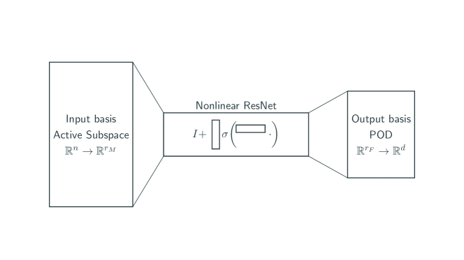
Recent research has motivated the deployment of neural networks as surrogates for parametric PDE mappings BhattacharyaHosseiniKovachki2020 ; FrescaManzoni2022 ; KovachkiLiLiuEtAl2021 ; LiKovachkiAzizzadenesheliEtAl2020b ; LuJinKarniadakis2019 ; OLearyRoseberryChenVillaEtAl2022 ; NelsenStuart21 ; NguyenBui2021model ; OLearyRoseberryVillaChenEtAl2022 . These surrogates can be used to accelerate the computation of the EIG within OED problems. Specifically, to reduce the prohibitive computational cost, we build a surrogate for the parameter-to-observable map at all candidate sensor locations by a derivative-informed projected neural network (DIPNet) OLearyRoseberry2020 ; OLearyRoseberryDuChaudhuriEtAl2021 ; OLearyRoseberryVillaChenEtAl2022 . Often, PDE-constrained high-dimensional parametric maps, such as the parameter-to-observable map , admit low-dimensional structure due to the correlation of the high-dimensional parameters, the regularizing property of the underlying PDE solution, and/or redundant information in the data from all candidate sensors. When this is the case, the DIPNet can exploit this low-dimensional structure and parametrize a parsimonious map between the most informed subspaces of the input parameter and the output observables. The dimensions of the input and output subspaces are referred to as the “information dimension” of the map, which is often significantly smaller than the parameter and data dimensions. The architectural strategy that we employ exploits compressibility of the map, by first reducing the input and output dimensionality via projection to informed reduced bases of the inputs and outputs. A neural network is then used to construct a low-dimensional nonlinear mapping between the two reduced bases. Error bounds for the effects of basis truncation, and parametrization by neural network are studied in BhattacharyaHosseiniKovachki2020 ; OLearyRoseberryDuChaudhuriEtAl2021 ; OLearyRoseberryVillaChenEtAl2022 .
For the input parameter dimension reduction, we use a vector generalization of an active subspace (AS) ZahmConstantinePrieurEtAl2020 , which is spanned by the generalized eigenvectors (input reduced basis) corresponding to the largest eigenvalues of the eigenvalue problem
| (19) |
where the eigenvectors are ordered by the decreasing generalized eigenvalues , . For the output data dimension reduction, we use a proper orthogonal decomposition (POD)ManzoniNegriQuarteroni2016 ; QuarteroniManzoniNegri2015 , which uses the eigenvectors (output reduced basis) corresponding to the first eigenvalues of the expected observable outer product matrix,
| (20) |
where the eigenvectors are ordered by the decreasing eigenvalues , . When the eigenvalues of AS and POD both decay quickly, the mapping can be well approximated when and are projected to the corresponding subspaces with small and ; in this case approximation error bounds for reduced basis representation of the mapping are given by the trailing eigenvalues of the systems (19),(20). This allows one to detect appropriate “breadth” for the neural network via the direct computation of the associated eigenvalue problems, removing the need for ad-hoc neural network hyperparameter search for appropriate breadth. The neural network surrogate of the map then has the form
| (21) |
where represents the POD reduced basis for the output, represents the AS reduced basis for the input, is the neural network mapping between the two bases parametrized by weights and bias . Since the reduced basis dimensions are chosen based on spectral decay of the AS and POD operators, we can choose them to be the same; for convenience we denote the reduced basis dimension instead by . The remaining difficulty is how to properly parametrize and train the neural network mapping. While the use of the reduced basis representation for the approximating map allows one to detect appropriate breadth for the neural network by avoiding complex neural network hyperparameter searches, and associated nonconvex neural network trainings, how to choose appropriate depth for the network is still an open question. While neural network approximation theory suggests deeper networks have richer representative capacities, in practice, for many architectures, adding depth eventually diminishes performance in what is known as the “peaking phenomenon”Hughes1968 . In general finding appropriate depth for e.g., fully-connected feedforward neural networks requires re-training from scratch different networks with differing depths. In order to avoid this issue we employ an adaptively constructed residual network (ResNet) neural network parametrization of the mapping between the two reduced bases. This adaptive construction procedure is motivated by recent approximation theory that conceives of ResNets as discretizations of sequentially minimizing control flows LiLinShen22 , where such maps are proven to be universal approximators of functions on compact sets. A schematic for our neural network architecture can be seen in Fig. 1.
This strategy adaptively constructs and trains a sequence of low-rank ResNet layers, where for convenience we take or otherwise employ a restriction or prolongation layer to enforce dimensional compatibility. The ResNet hidden neurons at layer have the form
| (22) |
with , , where the parameter is referred to as the layer rank, and it is chosen to be smaller than in order to impose a compressed representation of the ResNet latent space update (22). This choice is guided by the “well function” property in LiLinShen22 . The ResNet weights consist of all of the coefficient arrays in each layer. Given appropriate reduced bases with dimension , the ResNet mapping between the reduced bases is trained adaptively, one layer at a time, until over-fitting is detected in training validation metrics. When this is the case, a final global end-to-end training is employed using a stochastic Newton optimizer OLearyRoseberryAlgerGhattas2020 . This architectural strategy is able to achieve high generalizability for few and (input-output) dimension-independent data, for more information on this strategy, please see OLearyRoseberryDuChaudhuriEtAl2021 .
By removing the dependence of the input-to-output map on their high-dimensional and uninformed subspaces (complement to the low-dimensional and informed subspaces), we can construct a neural network of small input and output size that requires few training data. Since these architectures are able to achieve high generalization accuracy with limited training data for parametric PDE maps, they are especially well suited to scalable EIG approximation, since they can be efficiently queried many times at no cost in PDE solves, and require few high fidelity PDE solutions for their construction.
3.3 DLMC with DIPNet surrogate
We propose to train a DIPNet surrogate for the parameter-to-observable map , so that can be approximated as
| (23) |
where we omitted a constant since it appears in both the numerator and denominator of the argument of the log in the expression for the EIG. To this end, we can formulate the approximate EIG with the DIPNet surrogate as
| (24) | ||||
| (25) | ||||
| (26) |
where are i.i.d. observation noise. Thanks to the DIPNet surrogate, the EIG can be evaluated at negligible cost (relating to PDE solver cost) for each given , and does not require any PDE solves.
3.4 Error analysis
Theorem 1.
We assume that the parameter-to-observable map and its surrogate are bounded as
| (27) |
Moreover, we assume that the generalization error of the DIPNet surrogate can be bounded by , i.e.,
| (28) |
Then the error in the approximation of the normalization constant by the DIPNet surrogate can be bounded by
| (29) |
for sufficiently large and some constants , . Moreover, the approximation error for the EIG can be bounded by
| (30) |
for some constant .
Proof: For notational simplicity, we omit the dependence of and on and write and . Note that the bounds (27) and (28) also hold for and since and are selection of some entries of and . By definition of in (18) and in (23), and the fact that for any , we have
where we used the Cauchy–Schwarz inequality in the last inequality with given by
| (31) |
For sufficiently large , we have that by and the assumption (27). Moreover, the error bound (29) holds by the assumption (28).
3.5 Greedy algorithm
With the DIPNet surrogate, the evaluation of the DLMC EIG defined in (26) does not involve any PDE solves. Thus to solve the optimization problem
| (36) |
we can directly use a greedy algorithm that requires evaluations of the EIG, not its derivative w.r.t. . Let denote the set of all candidate sensors; we wish to choose sensors from that maximize the approximate EIG (approximated with the DIPNet surrogate). At the first step with , we select the sensor corresponding to the maximum approximate EIG and set . Then at step , with sensors selected in , we choose the -th sensor corresponding to the maximum approximate EIG evaluated with sensors ; see Algorithm 1 for the greedy optimization process, which can achieve (quasi-optimal) experimental designs with an approximation guarantee under suitable assumptions on the incremental information gain of an additional sensor; see JagalurMohanMarzouk21 and references therein. Note that at each step the approximate EIG can be evaluated in parallel for each sensor choice with .
4 Numerical results
In this section, we present numerical results for OED problems involving a Helmholtz acoustic inverse scattering problem and an advection-reaction-diffusion inverse transport problem to illustrate the efficiency and accuracy of our method. We compare the approximated normalization constant and EIG of our method with 1) the DLMC truth computed by a large number of Monte Carlo samples; and 2) the DLMC sampled at the same computational cost (number of PDE solves) as our method using DIPNet training.
Both PDE problems are discretized using the finite element library FEniCS AlnaesBlechtaHakeEtAl2015 . The construction of training data and reduced bases (active subspace and proper orthogonal decomposition) is implemented in hIPPYflow hippyflow , a library for dimension reduced PDE surrogate construction, building on top of PDE adjoints implemented in hIPPYlib VillaPetraGhattas20 . The DIPNet neural network surrogates are constructed in TensorFlow AbadiBarhanChenEtAl2016 , and are adaptively trained using a combination of Adam KingmaBa2014 , and a Newton method, LRSFN, which improves local convergence and generalization OLearyRoseberryAlgerGhattas2019 ; OLearyRoseberryAlgerGhattas2020 ; OLearyRoseberryDuChaudhuriEtAl2021 .
4.1 Helmholtz problem
For the first numerical experiment, we consider an inverse wave scattering problem modeled by the Helmholtz equation with uncertain medium in the two-dimensional physical domain
| (37a) | ||||
| PML boundary condition | (37b) | |||
| (37c) | ||||
| (37d) | ||||
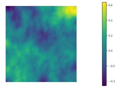
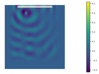
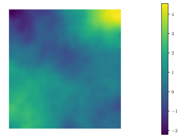
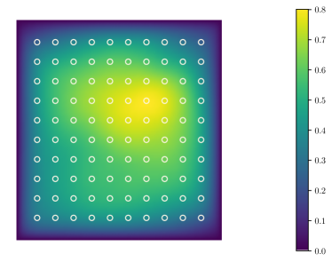
where is the total wave field, is the wavenumber, and models the uncertainty of the medium, with the parameter a log-prefactor of the squared wavenumber. The right hand side is a point source located at . The perfectly matched layer (PML) boundary condition approximates a semi-infinite domain. The candidate sensor locations are linearly spaced in the line segment between the edge points and , with coordinates , as shown in Fig. 2. The prior distribution for the uncertain parameter is Gaussian with zero mean and covariance . The mesh used for this problem is uniform of size . We use quadratic elements for the discretization of the wave field and linear elements for the parameter , leading to a discrete parameter of dimension . The dimension of the wave field is , the wave is more than sufficiently resolved in regards to the Nyquist sampling criteria for wave problems. A sample of the parameter field and the PDE solution is shown in Fig. 2 with all candidate sensor locations marked in circles.
The network has low-rank residual layers, each with a layer rank of . For this numerical example we demonstrate the effects of using different breadths in the neural network representation, in each case the ResNet learns a mapping from the first basis vectors for active subspace to the first basis vectors of POD. In the case that we use a linear restriction layer to reduce the ResNet latent representation to the dimensional output. For the majority of the numerical results, we employ a dimensional network. The neural network is trained adaptively using training samples, and validation samples. Using independent testing samples, the DIPNet surrogate was accurate measured as a percentage by
| (38) |
For more details on this neural network architecture and training, see OLearyRoseberryDuChaudhuriEtAl2021 . The computational cost of the dimensional active subspace projector using samples is equivalent to the cost of additional training data; since the problem is linear the additional linear adjoint computations are comparable to the costs of the training data generation. As we will see in the next example, when the PDE is nonlinear the additional active subspace computations are marginal. Thus for fair comparison with the same computational cost of PDE solves, we use samples for simple MC.
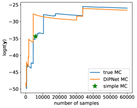
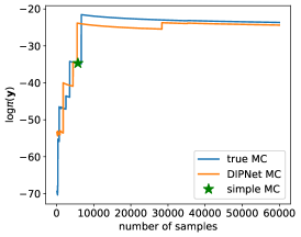
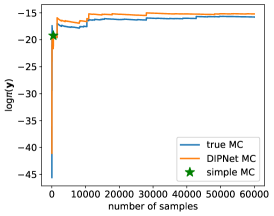
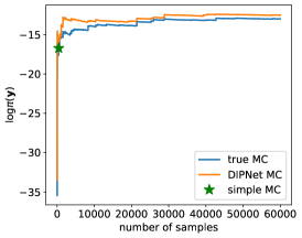
To test the efficiency and accuracy of our DIPNet surrogate, we first compute the log normalization constant with our DIPNet surrogate for given observation data generated by . is a random sample from the prior. We use in total random samples for Monte Carlo (MC) to compute the normalization constant as the ground truth. Fig. 3 shows the comparison for three random designs that choose sensors out of candidates. We can see that DIPNet surrogate converges to a value close to the ground truth MC reference, while for the (simple) MC with samples, the approximated value indicated by the green star is much less accurate than the DIPNet surrogate using samples with similar cost in PDE solves. Note that the DIPNet training and evaluation cost for this small size neural network is negligible compared to PDE solves.
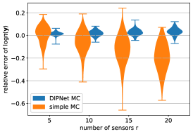
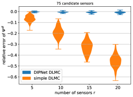
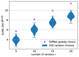
The left and middle figures in Fig. 4 illustrate the sample distributions of the relative approximation errors for the log normalization constant and the EIG () with (DIPNet MC with samples) and without (simple MC with samples) the DIPNet surrogate, compared to the true MC with samples. These results show that using DIPNet surrogate we can approximate and much more accurately with less bias compared to the simple MC. The sample distributions of EIG at random designs compared to the design chosen by the greedy optimization using DIPNet surrogate for different number of sensors are shown in the right figure, from which we can see that our method can always chose better designs with larger EIG values than all the random designs.
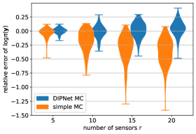
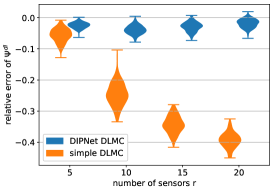
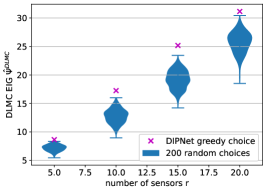
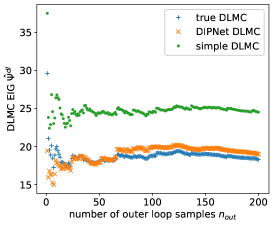
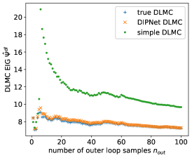
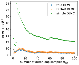
Fig. 5 gives approximate values of the EIG with increasing number of outer loop samples using: the DIPNet surrogate with inner loop , simple DLMC with inner loop , and the truth computed with inner loop . We can see that the approximate values by the DIPNet surrogates are almost the same as the truth, while simple DLMC results are very inaccurate.
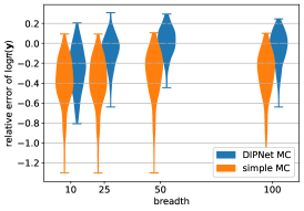
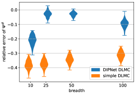
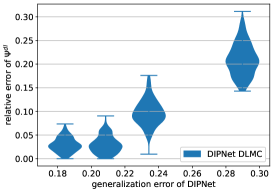
To show the effectiveness of truncated rank (breadth) for DIPNet surrogate, we evaluate the log normalization constant and EIG with breadth and compared with true MC and simple MC in Fig. 6. We can see that with increasing breadth, the relative error is decreasing, but gets worse when breadth reaches . With breadth , the difficulties of neural network training start to dominate and diminish the accuracy. We can also see it in the right part of the figure. The relative error of EIG approximation reduces (close to) linearly with respect to the generalization error of the DIPNet approximation of the observables with network breadth , which confirms the error analysis in Theorem 1. However, when the breadth increases to , the neural network becomes less accurate (without using more training data), leading to less accurate EIG approximation.
4.2 Advection-diffusion-reaction problem
For the second numerical experiment we consider an OED problem for an advection-diffusion-reaction equation with a cubic nonlinear reaction term. The uncertain parameter appears as a log-coefficient of the cubic nonlinear reaction term. The PDE is defined in a domain as
| (39a) | ||||
| (39b) | ||||
| (39c) | ||||
Here is the diffusion coefficient. The volumetric forcing function f is a smoothed Gaussian bump located at ,
| (40) |
The velocity field is a solution of a steady-state Navier Stokes equation with shearing boundary conditions driving the flow (see the Appendix in OLearyRoseberryVillaChenEtAl2022 for more information on the flow). The candidate sensor locations are located in a linearly spaced mesh-grid of points in , with coordinates . The prior distribution for the uncertain parameter is a mean zero Gaussian with covariance . The mesh used for this problem is uniform of size . We use linear elements for both and , leading to a discrete parameter of dimension . Fig. 7 gives a prior sample of the parameter field and the solution with all candidate sensor locations in white circles.
The neural network surrogate is trained adaptively using training samples and validation samples. Using independent testing samples the DIPNet network was accurate (see equation 38). The network has low-rank residual layers, each with a layer rank of , the breadth of the network is . The computational cost of the dimensional active subspace projector using samples is equivalent to the cost of additional training data. As was noted before when the PDE is nonlinear the linear adjoint-based derivative computations become much less of a computational burden. Thus we use samples for simple MC for fair comparison.
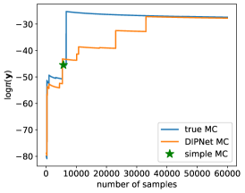
We first examine the log normalization constant computed with our PDE-solve-based DIPNet surrogate compared against the truth computed with MC samples and the simple MC computed with samples. Fig. 8 shows the comparison for three random designs that select sensors out of candidates. We can see that DIPNet MC converges to a value close to the true MC curves, while the simple MC’s green star computed with the same number of PDE solves () as DIPNet MC, has much worse accuracy.

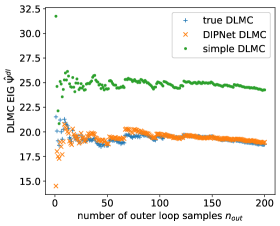
The left figure of Fig. 9 shows the relative errors for computed with the DIPNet surrogate and simple MC using samples based on the true MC with samples, for random designs. We see again that DIPNet gives better accuracy with less bias than simple MC.
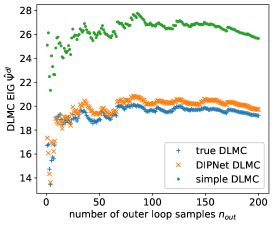
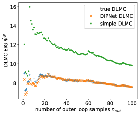
Fig. 10 shows the EIG approximations of three random designs with increasing number of outer loop samples using the DIPNet MC with (inner loop) samples, simple MC with samples, and true MC with samples. We can see that the values of DIPNet MC are quite close to the true MC, while simple MC is far off. Relative errors of the EIG () computed with the DIPNet surrogate, the simple MC for random designs is given in the middle figure of Fig. 9. With the DIPNet DLMC , we can use the greedy algorithm to find the optimal designs. The DIPNet greedy designs are presented as the pink crosses in the right figure of Fig. 9. We can see that the designs chosen by the greedy algorithm have much larger EIG values than all random designs.
5 Conclusions
We have developed a computational method based on DIPNet surrogates for solving large-scale PDE-constrained Bayesian OED problems to determine optimal sensor locations (using the EIG criterion) to best infer infinite-dimensional parameters. We exploited the intrinsic low dimensionality of the parameter and data spaces and constructed a DIPNet surrogate for the parameter-to-observable map. The surrogate was used repeatedly in the evaluation of the normalization constant and the EIG. We presented error analysis for the approximation of the normalization constant and the EIG, showing that the errors are of the same order as the DIPNet RMS approximation error. Moreover, we used a greedy algorithm to solve the combinatorial optimization problem for sensor selection. The computational efficiency and accuracy of our approach are demonstrated by two numerical experiments. Future work will focus on gradient-based optimization also using the derivative information of the DIPNet w.r.t. both the parameter and the design variables, on the use of different optimality criteria such as A-optimality or D-optimality, and on exploring new network architectures for intrinsically high-dimensional Bayesian OED problems.
References
- \bibcommenthead
- (1) Uciński, D.: Optimal Measurement Methods for Distributed Parameter System Identification. CRC Press, Boca Raton (2005)
- (2) Loose, N., Heimbach, P.: Leveraging uncertainty quantification to design ocean climate observing systems. Journal of Advances in Modeling Earth Systems, 1–29 (2021)
- (3) Ferrolino, A.R., Lope, J.E.C., Mendoza, R.G.: Optimal location of sensors for early detection of tsunami waves. In: International Conference on Computational Science, pp. 562–575 (2020). Springer
- (4) Huan, X., Marzouk, Y.M.: Simulation-based optimal Bayesian experimental design for nonlinear systems. Journal of Computational Physics 232(1), 288–317 (2013). https://doi.org/10.1016/j.jcp.2012.08.013
- (5) Huan, X., Marzouk, Y.M.: Gradient-based stochastic optimization methods in Bayesian experimental design. International Journal for Uncertainty Quantification 4(6), 479–510 (2014)
- (6) Huan, X., Marzouk, Y.M.: Sequential bayesian optimal experimental design via approximate dynamic programming. arXiv preprint arXiv:1604.08320 (2016)
- (7) Alexanderian, A., Petra, N., Stadler, G., Ghattas, O.: A fast and scalable method for A-optimal design of experiments for infinite-dimensional Bayesian nonlinear inverse problems. SIAM Journal on Scientific Computing 38(1), 243–272 (2016). https://doi.org/10.1137/140992564
- (8) Beck, J., Dia, B.M., Espath, L.F., Long, Q., Tempone, R.: Fast bayesian experimental design: Laplace-based importance sampling for the expected information gain. Computer Methods in Applied Mechanics and Engineering 334, 523–553 (2018). https://doi.org/10.1016/j.cma.2018.01.053
- (9) Long, Q., Scavino, M., Tempone, R., Wang, S.: Fast estimation of expected information gains for Bayesian experimental designs based on Laplace approximations. Computer Methods in Applied Mechanics and Engineering 259, 24–39 (2013)
- (10) Long, Q., Motamed, M., Tempone, R.: Fast bayesian optimal experimental design for seismic source inversion. Computer Methods in Applied Mechanics and Engineering 291, 123–145 (2015). https://doi.org/10.1016/j.cma.2015.03.021
- (11) Beck, J., Mansour Dia, B., Espath, L., Tempone, R.: Multilevel double loop Monte Carlo and stochastic collocation methods with importance sampling for Bayesian optimal experimental design. International Journal for Numerical Methods in Engineering 121(15), 3482–3503 (2020)
- (12) Alexanderian, A., Petra, N., Stadler, G., Ghattas, O.: A-optimal design of experiments for infinite-dimensional Bayesian linear inverse problems with regularized -sparsification. SIAM Journal on Scientific Computing 36(5), 2122–2148 (2014). https://doi.org/10.1137/130933381
- (13) Alexanderian, A., Gloor, P.J., Ghattas, O.: On Bayesian A-and D-optimal experimental designs in infinite dimensions. Bayesian Analysis 11(3), 671–695 (2016). https://doi.org/10.1214/15-BA969
- (14) Saibaba, A.K., Alexanderian, A., Ipsen, I.C.: Randomized matrix-free trace and log-determinant estimators. Numerische Mathematik 137(2), 353–395 (2017)
- (15) Crestel, B., Alexanderian, A., Stadler, G., Ghattas, O.: A-optimal encoding weights for nonlinear inverse problems, with application to the Helmholtz inverse problem. Inverse Problems 33(7), 074008 (2017)
- (16) Attia, A., Alexanderian, A., Saibaba, A.K.: Goal-oriented optimal design of experiments for large-scale Bayesian linear inverse problems. Inverse Problems 34(9), 095009 (2018)
- (17) Wu, K., Chen, P., Ghattas, O.: A fast and scalable computational framework for large-scale and high-dimensional Bayesian optimal experimental design. arXiv preprint arXiv:2010.15196, to appear in SIAM Journal on Scientific Computing (2020)
- (18) Wu, K., Chen, P., Ghattas, O.: An efficient method for goal-oriented linear bayesian optimal experimental design: Application to optimal sensor placement. arXiv preprint arXiv:2102.06627, to appear in SIAM/AMS Journal on Uncertainty Quantification (2021)
- (19) Aretz-Nellesen, N., Chen, P., Grepl, M.A., Veroy, K.: A-optimal experimental design for hyper-parameterized linear Bayesian inverse problems. Numerical Mathematics and Advanced Applications ENUMATH 2020 (2020)
- (20) Aretz, N., Chen, P., Veroy, K.: Sensor selection for hyper-parameterized linear Bayesian inverse problems. PAMM 20(S1), 202000357 (2021)
- (21) Foster, A., Jankowiak, M., Bingham, E., Horsfall, P., Teh, Y.W., Rainforth, T., Goodman, N.: Variational Bayesian optimal experimental design. In: Wallach, H., Larochelle, H., Beygelzimer, A., d' Alché-Buc, F., Fox, E., Garnett, R. (eds.) Advances in Neural Information Processing Systems, vol. 32, pp. 14036–14047. Curran Associates, Inc., ??? (2019). https://proceedings.neurips.cc/paper/2019/file/d55cbf210f175f4a37916eafe6c04f0d-Paper.pdf
- (22) Kleinegesse, S., Gutmann, M.U.: Bayesian experimental design for implicit models by mutual information neural estimation. In: International Conference on Machine Learning, pp. 5316–5326 (2020). PMLR
- (23) Shen, W., Huan, X.: Bayesian sequential optimal experimental design for nonlinear models using policy gradient reinforcement learning. arXiv preprint arXiv:2110.15335 (2021)
- (24) O’Leary-Roseberry, T., Villa, U., Chen, P., Ghattas, O.: Derivative-informed projected neural networks for high-dimensional parametric maps governed by pdes. Computer Methods in Applied Mechanics and Engineering 388, 114199 (2022)
- (25) O’Leary-Roseberry, T.: Efficient and dimension independent methods for neural network surrogate construction and training. PhD thesis, The University of Texas at Austin (2020)
- (26) O’Leary-Roseberry, T., Du, X., Chaudhuri, A., Martins, J.R., Willcox, K., Ghattas, O.: Adaptive projected residual networks for learning parametric maps from sparse data. arXiv preprint arXiv:2112.07096 (2021)
- (27) Flath, P.H., Wilcox, L.C., Akçelik, V., Hill, J., van Bloemen Waanders, B., Ghattas, O.: Fast algorithms for Bayesian uncertainty quantification in large-scale linear inverse problems based on low-rank partial Hessian approximations. SIAM Journal on Scientific Computing 33(1), 407–432 (2011). https://doi.org/10.1137/090780717
- (28) Bui-Thanh, T., Burstedde, C., Ghattas, O., Martin, J., Stadler, G., Wilcox, L.C.: Extreme-scale UQ for Bayesian inverse problems governed by PDEs. In: SC12: Proceedings of the International Conference for High Performance Computing, Networking, Storage and Analysis (2012)
- (29) Bui-Thanh, T., Ghattas, O., Martin, J., Stadler, G.: A computational framework for infinite-dimensional Bayesian inverse problems Part I: The linearized case, with application to global seismic inversion. SIAM Journal on Scientific Computing 35(6), 2494–2523 (2013). https://doi.org/10.1137/12089586X
- (30) Bui-Thanh, T., Ghattas, O.: An analysis of infinite dimensional Bayesian inverse shape acoustic scattering and its numerical approximation. SIAM/ASA Journal of Uncertainty Quantification 2(1), 203–222 (2014). https://doi.org/10.1137/120894877
- (31) Kalmikov, A.G., Heimbach, P.: A Hessian-based method for uncertainty quantification in global ocean state estimation. SIAM Journal on Scientific Computing 36(5), 267–295 (2014)
- (32) Hesse, M., Stadler, G.: Joint inversion in coupled quasistatic poroelasticity. Journal of Geophysical Research: Solid Earth 119(2), 1425–1445 (2014)
- (33) Isaac, T., Petra, N., Stadler, G., Ghattas, O.: Scalable and efficient algorithms for the propagation of uncertainty from data through inference to prediction for large-scale problems, with application to flow of the Antarctic ice sheet. Journal of Computational Physics 296, 348–368 (2015). https://doi.org/%****␣manuscript.bbl␣Line␣550␣****10.1016/j.jcp.2015.04.047
- (34) Cui, T., Law, K.J.H., Marzouk, Y.M.: Dimension-independent likelihood-informed MCMC. Journal of Computational Physics 304, 109–137 (2016)
- (35) Chen, P., Villa, U., Ghattas, O.: Hessian-based adaptive sparse quadrature for infinite-dimensional Bayesian inverse problems. Computer Methods in Applied Mechanics and Engineering 327, 147–172 (2017)
- (36) Beskos, A., Girolami, M., Lan, S., Farrell, P.E., Stuart, A.M.: Geometric MCMC for infinite-dimensional inverse problems. Journal of Computational Physics 335, 327–351 (2017)
- (37) Zahm, O., Cui, T., Law, K., Spantini, A., Marzouk, Y.: Certified dimension reduction in nonlinear Bayesian inverse problems. arXiv preprint arXiv:1807.03712 (2018)
- (38) Brennan, M., Bigoni, D., Zahm, O., Spantini, A., Marzouk, Y.: Greedy inference with structure-exploiting lazy maps. Advances in Neural Information Processing Systems 33 (2020)
- (39) Chen, P., Wu, K., Chen, J., O’Leary-Roseberry, T., Ghattas, O.: Projected Stein variational Newton: A fast and scalable Bayesian inference method in high dimensions. Advances in Neural Information Processing Systems (2019)
- (40) Chen, P., Ghattas, O.: Projected Stein variational gradient descent. In: Advances in Neural Information Processing Systems (2020)
- (41) Subramanian, S., Scheufele, K., Mehl, M., Biros, G.: Where did the tumor start? An inverse solver with sparse localization for tumor growth models. Inverse Problems 36(4), 045006 (2020). https://doi.org/10.1088/1361-6420/ab649c
- (42) Babaniyi, O., Nicholson, R., Villa, U., Petra, N.: Inferring the basal sliding coefficient field for the Stokes ice sheet model under rheological uncertainty. The Cryosphere 15(4), 1731–1750 (2021)
- (43) Ghattas, O., Willcox, K.: Learning physics-based models from data: perspectives from inverse problems and model reduction. Acta Numerica 30, 445–554 (2021). https://doi.org/10.1017/S0962492921000064
- (44) Stuart, A.M.: Inverse problems: A Bayesian perspective. Acta Numerica 19, 451–559 (2010). https://doi.org/10.1017/S0962492910000061
- (45) Petra, N., Martin, J., Stadler, G., Ghattas, O.: A computational framework for infinite-dimensional Bayesian inverse problems: Part II. Stochastic Newton MCMC with application to ice sheet flow inverse problems. SIAM Journal on Scientific Computing 36(4), 1525–1555 (2014)
- (46) Bhattacharya, K., Hosseini, B., Kovachki, N.B., Stuart, A.M.: Model reduction and neural networks for parametric pdes. arXiv preprint arXiv:2005.03180 (2020)
- (47) Fresca, S., Manzoni, A.: POD-DL-ROM: enhancing deep learning-based reduced order models for nonlinear parametrized pdes by proper orthogonal decomposition. Computer Methods in Applied Mechanics and Engineering 388, 114181 (2022)
- (48) Kovachki, N., Li, Z., Liu, B., Azizzadenesheli, K., Bhattacharya, K., Stuart, A., Anandkumar, A.: Neural operator: Learning maps between function spaces. arXiv preprint arXiv:2108.08481 (2021)
- (49) Li, Z., Kovachki, N., Azizzadenesheli, K., Liu, B., Bhattacharya, K., Stuart, A., Anandkumar, A.: Neural operator: Graph kernel network for partial differential equations. arXiv preprint arXiv:2003.03485 (2020)
- (50) Lu, L., Jin, P., Karniadakis, G.E.: Deeponet: Learning nonlinear operators for identifying differential equations based on the universal approximation theorem of operators. arXiv preprint arXiv:1910.03193 (2019)
- (51) O’Leary-Roseberry, T., Chen, P., Villa, U., Ghattas, O.: Derivative-Informed Neural Operator: An Efficient Framework for High-Dimensional Parametric Derivative Learning. arXiv preprint arXiv:2206.10745 (2022)
- (52) Nelsen, N.H., Stuart, A.M.: The random feature model for input-output maps between banach spaces. SIAM Journal on Scientific Computing 43(5), 3212–3243 (2021)
- (53) Nguyen, H.V., Bui-Thanh, T.: Model-constrained deep learning approaches for inverse problems. arXiv preprint arXiv:2105.12033 (2021)
- (54) Zahm, O., Constantine, P.G., Prieur, C., Marzouk, Y.M.: Gradient-based dimension reduction of multivariate vector-valued functions. SIAM Journal on Scientific Computing 42(1), 534–558 (2020)
- (55) Manzoni, A., Negri, F., Quarteroni, A.: Dimensionality reduction of parameter-dependent problems through proper orthogonal decomposition. Annals of Mathematical Sciences and Applications 1(2), 341–377 (2016)
- (56) Quarteroni, A., Manzoni, A., Negri, F.: Reduced Basis Methods for Partial Differential Equations: An Introduction vol. 92. Springer, ??? (2015)
- (57) Hughes, G.: On the mean accuracy of statistical pattern recognizers. IEEE transactions on information theory 14(1), 55–63 (1968)
- (58) Li, Q., Lin, T., Shen, Z.: Deep learning via dynamical systems: An approximation perspective. Journal of the European Mathematical Society (2022)
- (59) O’Leary-Roseberry, T., Alger, N., Ghattas, O.: Low rank saddle free Newton: A scalable method for stochastic nonconvex optimization. arXiv preprint arXiv:2002.02881 (2020)
- (60) Jagalur-Mohan, J., Marzouk, Y.: Batch greedy maximization of non-submodular functions: Guarantees and applications to experimental design. Journal of Machine Learning Research 22(252), 1–62 (2021)
- (61) Alnæs, M.S., Blechta, J., Hake, J., Johansson, A., Kehlet, B., Logg, A., Richardson, C., Ring, J., Rognes, M.E., Wells, G.N.: The FEniCS project version 1.5. Archive of Numerical Software 3(100) (2015). https://doi.org/10.11588/ans.2015.100.20553
- (62) O’Leary-Roseberry, T., Villa, U.: hippyflow: Dimension reduced surrogate construction for parametric PDE maps in Python (2021). https://doi.org/10.5281/zenodo.4608729
- (63) Villa, U., Petra, N., Ghattas, O.: hIPPYlib: An extensible software framework for large-scale inverse problems governed by PDEs; Part I: Deterministic inversion and linearized Bayesian inference. ACM Transactions on Mathematical Software (2021)
- (64) Abadi, M., Barham, P., Chen, J., Chen, Z., Davis, A., Dean, J., Devin, M., Ghemawat, S., Irving, G., Isard, M., et al.: Tensorflow: A system for large-scale machine learning. In: 12th USENIX Symposium on Operating Systems Design and Implementation (OSDI 16), pp. 265–283 (2016)
- (65) Kingma, D.P., Ba, J.: Adam: A method for stochastic optimization. arXiv preprint arXiv:1412.6980 (2014)
- (66) O’Leary-Roseberry, T., Alger, N., Ghattas, O.: Inexact Newton methods for stochastic nonconvex optimization with applications to neural network training. arXiv preprint arXiv:1905.06738 (2019)