Deep self-consistent learning of local volatility

Abstract

We present an algorithm for the calibration of local volatility from market option prices through deep self-consistent learning, by approximating both market option prices and local volatility using deep neural networks, respectively. Our method uses the initial-boundary value problem of the underlying Dupire’s partial differential equation solved by the parameterized option prices to bring corrections to the parameterization in a self-consistent way. By exploiting the differentiability of the neural networks, we can evaluate Dupire’s equation locally at each strike-maturity pair; while by exploiting their continuity, we sample strike-maturity pairs uniformly from a given domain, going beyond the discrete points where the options are quoted. Moreover, the absence of arbitrage opportunities are imposed by penalizing an associated loss function as a soft constraint. For comparison with existing approaches, the proposed method is tested on both synthetic and market option prices, which shows an improved performance in terms of reduced interpolation and reprice errors, as well as the smoothness of the calibrated local volatility. An ablation study has been performed, asserting the robustness and significance of the proposed method.

Keywords: Local volatility, deep self-consistent learning, Dupire PDE.

1 Introduction

Local volatility provides a measure for the risk of financial markets. Consequently, it is an important input widely used in quantitative finance to compute, for instance, quotes for market makers, margin requirements for brokers, prices of exotic derivatives for quants, and strategies positions for traders [ATV20]. Therefore, a small calibration error in local volatility can lead to a dramatic change in investment strategy and, eventually, a huge financial loss.

However, local volatility cannot be directly measured; it is usually calibrated from the quoted option prices available in the market. An option is a financial contract that gives options holders the right but not the obligation to buy (a call option) or to sell (a put option) an asset, e.g. stocks or commodity, for a predetermined price (strike price) on a predetermined date (maturity). To acquire today the right to buy or sell an asset in the future, a premium must be paid to the option writers, namely the option price. The standard approach to model option price is based on the Black-Scholes formula, which assumes a constant local volatility surface, hence it is applicable only to situations where the stock prices process follows the geometric Brownian motion. Options are traded on financial exchanges, and the prices of the underlying assets typically invalidate the assumption of standard Brownian motion, hence a more sophisticated model than the Black-Scholes formula is required. Among alternatives, we consider an asset price process expressed in a local volatility model as

$$dS_{t}=rS_{t}dt+\sigma(S_{t},t)S_{t}dB_{t},\quad S_{t}|_{t=0}=S_{0}.$$ (1)

where $S_{t}$ denotes the stock price at the time $t\in\mathbb{R}_{+}$ and $B_{t}$ is a standard Brownian motion. For simplicity, we assume a zero dividend yield and a constant risk-free interest rate $r$. Rather than a constant value as in the canonical Black-Scholes equation, in Eq. (1), the local volatility $\sigma(S_{t},t)$ is a deterministic function of the underlying asset price $S_{t}$ and of time $t$, satisfying the usual Lipschitz conditions. Without introducing additional sources of randomness, the local volatility model is the only complete and consistent model that allows hedging based on solely the underlying asset and containing no contradiction, cf. Appendix A1 in [Ben14]; and it is used by $90\%$ of investment banks’ production systems in daily risk management.

The practical implementation of such a stochastic volatility model in option pricing requires to solve a challenging problem of calibrating the local volatility function to the market data of option prices. Given $\pi(K,T)$ a family of option prices with strike prices $K>0$, maturities $T>0$, and underlying asset price $S_{0}=x$, the Dupire formula [Dup94, DK94]

$$\sigma(K,T):=\sqrt{\displaystyle\frac{\displaystyle 2\frac{\partial\pi}{\partial T}(K,T)+2rK\frac{\partial\pi}{\partial K}(K,T)}{\displaystyle K^{2}\frac{\partial^{2}\pi}{\partial K^{2}}(K,T)}},$$ (2)

brings a solution to this problem by constructing an estimator of the local volatility as a function of strike price $K$ and maturity $T$ values, i.e. Eq. (2) matches the stock’s volatility $\sigma(S_{t},t)$ when the future stock price is $K$ at time $T$.

The numerical estimation of local volatility using Eq. (2), involves evaluating partial derivatives, which is classically achieved using the finite difference method. More efficient methods have been introduced using spline functions, see e.g. Chapter 8 in [AP05], where local volatility is first approximated as the sum a piece-wise affine function satisfying a boundary condition and a bi-cubic spline function. Then, the model parameters are determined by minimizing the discretized Dupire’s equations [Dup94] at selected collocation points with Tikhonov regularization. Thereafter, Tikhonov regularization has been applied to the calibration of local volatility in a trinomial model in [Cré02].

Alternative to calibrating local volatility using parameterized functions, neural networks are known being able to approximate any arbitrary nonlinear function with a finite set of parameters [GW98, WL17, LJ18]. Exploiting recent advance in deep learning, Chataigner et al. [CCD20] advocated to parameterize market option prices $\pi(K,T)$ with a neural network. As neural networks are differentiable functions, the derivatives in Eq. (2) are computed using automatic differentiation [BPRS17]. For Dupire’s formula to be meaningful, one must ensure that the argument in the square root is positive and remains bounded. Together with a requirement that the quoted option prices are arbitrage-free, one imposes additional constraints when fitting the option prices as in [CCD20]. As soon as the market option prices are well fitted, an approximation of derivatives of the option price is then substituted into Eq. (2) to calibrate the local volatility. Consequently, the quality of the reconstructed local volatility surface depends on the resolution and quality of the quoted market option prices at given strike-maturity pairs. Instead of using market option price, Chataigner et al. [CCC⁺21] proposed, subsequently, to calibrate local volatility from the implied volatility surface, leading to an improved performance. It is, however, important to note that, when fitting option prices or implied volatilities using neural networks, one assume that the data are noise free. Except for those violates arbitrage-free conditions, the proposed methods in [CCD20, CCC⁺21] are not able to filter out noises in the data.

In this work, we adopt the idea in [WG22] and calibrate the local volatility surface from the observed market option prices in a self-consistent manner. Going beyond merely fitting option prices using neural networks, we rely on recent studies on physics-informed machine learning [RPK19, RMM⁺20, KKL⁺21, WG22] which have shown that the inclusion of residue of an unknown, underlying governing equation as a regularizer can not only calibrate the unknown terms in the governing equations, but also bring correction to the data by filtering out noises that are not characterized by the equation.

To begin with, we approximate both the market option prices and the squared local volatility using deep neural networks. By requiring that $\pi(K,T)$ is a solution to the Dupire equation subjected to given initial and boundary conditions to be discussed in Section 2.1, we regularize $\pi(K,T)$ and determine the unknown $\sigma(K,T)$ self-consistently. Since the resulting $\pi(K,T)$ and $\sigma(K,T)$ are continuous and differentiable functions of $K$ and $T$, this allows us to evaluate Dupire’s equation locally on a uniformly sampled $(K,T)$ from the support manifold of Dupire’s equation. Unlike previous approaches, where constraints were imposed on fixed strike-maturity pairs, a successive re-sampling enables us to regularize the entire support. In addition, the positiveness of $\sigma(K,T)$ is ensured by a properly selected output activation function of the neural network, hence it is everywhere well defined. Finally, we mitigate the risk of arbitrage opportunities by penalizing a loss as soft constraints.

The rest of the paper is organized as follows. We review in Section 2 of background knowledge including Dupire’s equation and arbitrage-free conditions, followed by a comment on the market data. After rescaling and reparameterization of market option prices in Section 3.1 and a discussion of neural ansatz and loss functions in Section 3.2, our deep self-consistent algorithm is summarized and discussed in Section 3.3. The proposed method is first tested on synthetic datasets in Section 4.1, and then applied to market option prices in Section 4.2 where, as an ablation study, we compare our results with those obtained without including the residue of Dupire’s equation as a regularizer. Finally, the advantages and limitations of our method are discussed in Section 5, where conclusions are drawn.

2 Background and objectives

2.1 Dupire’s equation

Denote by $\pi^{c}(K,T)$ and $\pi^{p}(K,T)$ the prices for European call and put options

$$\pi^{c}(K,T) =e^{-rT}\mathbb{E}\big{[}(S_{T}-K)^{+}\big{]},$$ (3a)

$$\pi^{p}(K,T) =e^{-rT}\mathbb{E}\big{[}(K-S_{T})^{+}\big{]},$$ (3b)

the relation between the market option price and the local volatility is established explicitly by Dupire’s equation [Dup94]

$$\frac{\partial\pi}{\partial T}(K,T)+rK\frac{\partial\pi}{\partial K}(K,T)-\frac{1}{2}K^{2}\sigma^{2}(K,T)\frac{\partial^{2}\pi}{\partial K^{2}}(K,T)=0,$$ (4)

subjected to the initial

$$\pi^{c}(K,0)=\left(S_{0}-K\right)^{+}\quad\mbox{or}\quad\pi^{p}(K,0)=\left(K-S_{0}\right)^{+},$$ (5)

and boundary

$$\quad\pi^{c}(\infty,T)=0\quad\mbox{or}\quad\pi^{p}(0,T)=0,$$ (6)

conditions for call and put options, respectively. We refer the readers to Chapter 1 in [Itk20] and to Proposition 9.2 in [Pri22] for a detailed derivation of Dupire’s equation, and to Chapter 8 in [AP05] for discussion on initial and boundary conditions. Stemming from their definitions (3), we conclude that the prices of European options are nonnegative, with the prices of call options being always less than the value of the underlying asset; while the prices of the put options being always less than the present value of the strike price, leading to the following lower and upper bounds

$$0\leq\pi^{c}(K,T)\leq S_{0}\quad\mbox{and}\quad 0\leq\pi^{p}(K,T)\leq K.$$ (7)

2.2 Arbitrage-free surface

A static arbitrage is a trading strategy that has zero value initially and it is always non-negative afterwards, representing a risk-free investment after accounting for transaction costs. Under the assumption that economic agents are rational, arbitrage opportunities, if they ever exist, will be instantaneously exploited until the market is arbitrage free. Therefore, as a prerequisite, the absence of arbitrage opportunities is a fundamental principle underpinning the modern theory of financial asset pricing. An option price surface is free of static arbitrage if and only if (i) each strike slice is free of calendar spread arbitrage; and (ii) each maturity slice is free of butterfly arbitrage [ATV20, CCD20, CCC⁺21]. Both calendar spread and butterfly arbitrages can be created with put options as well as call options, cf. Sec. 9.2 in [Hul03] for details. A calendar spread arbitrage is created by buying a long-maturity put option and selling a short-maturity put option. Hence, the zero calendar spread arbitrage implies, in the continuous limit, that

$$\frac{\partial\pi}{\partial T}(K,T)\geq 0.$$ (8)

A butterfly arbitrage can be created by buying two options at prices $K_{1}$ and $K_{3}$, with $K_{3}>K_{1}$; and selling two options with a strike price, $K_{2}=(K_{1}+K_{3})/2$. In the continuous limit, the absence of butterfly arbitrage leads to

$$\frac{\partial^{2}\pi}{\partial K^{2}}(K,T)\geq 0.$$ (9)

2.3 Problem formulation

Market option prices are observed on $N$ discrete pairs of strike price and maturity values, leading to triplets $(\pi_{i},K_{i},T_{i})$ with $i=1,...,N$. In practice, to secure a transaction, two option prices are quoted in the market, a bid and a ask prices, and there is no guarantee that the mid-price $\pi_{i}$ between the bid and ask prices is arbitrage-free [ATV20]. Moreover, the observed bid and ask prices may not be updated timely, hence not actionable, leading to additive noise to the market data. Lastly, market option prices are not evenly quoted over a plane spanned by $K$ and $T$: the market data are usually dense close to the money; whereas sparse away from the money. Canonical methods often lack the ability to interpolate option prices and calibrate the associated local volatility without quotes, agilely. Therefore, a validation, a correction, and an interpolation to the market data are required.

Consequently, the main challenge when calibrating the local volatility is twofold. First, given limited observations of unevenly distributed option prices quoted on discrete pairs of strikes and maturities, the calibrated local volatility should span a smooth manifold. Second, the corresponding option prices should preclude any arbitrage opportunities. Our objective is, therefore, to construct from observed market option prices a self-consistent approximation for both $\sigma(K,T)$ and $\pi(K,T)$ in the sense that the calibrated local volatility will generate an arbitrage-free option price surface that is in line with the market data up to some physics-informed corrections.

3 Methodology

3.1 Rescaling of Dupire’s equation

In this section, a change of variable and a rescaling is applied to Dupire’s equation (4). This is to ensure that terms in scaled Eq. (12) below are of order of unity, so that no term is dominating over the others during the minimization. For this, we introduce the following change of variables

$$k=e^{-rT}K/K_{\text{max}},\quad t=T/T_{\text{max}},$$ (10)

where Dupire’s equation is localized by picking sufficiently large $K_{\text{max}}$ and $T_{\text{max}}$. Without loss of generality, we take $K_{\text{max}}=\text{max}(K)$ and $T_{\text{max}}=\text{max}(T)$. Denote by

$$\eta(k,t)=\frac{T_{\text{max}}}{2}\sigma^{2}(K,T),$$ (11)

the squared local volatility, the Dupire’s equation (4) can be expressed as

$$f_{\text{dup}}(k,t):=\frac{\partial{\pi}}{\partial t}(k,t)-{\eta}(k,t)k^{2}\frac{\partial^{2}{\pi}}{\partial k^{2}}(k,t)=0,$$ (12)

subject to initial and boundary conditions

$${\pi}^{c}(k,0)=\big{(}S_{0}-K_{\text{max}}k\big{)}^{+},\quad{\pi}^{c}(\infty,t)=0,$$ (13)

for call option prices, and

$${\pi}^{p}(k,0)=\big{(}K_{\text{max}}k-S_{0}\big{)}^{+},\quad{\pi}^{p}(0,t)=0,$$ (14)

for put option prices, respectively, as well as the inequality constraints (7).

Using Eq. (12), the corresponding conditions for the absence of calendar

$$\frac{\partial\pi}{\partial T}(K,T)\propto\frac{\partial{\pi}}{\partial t}(k,t)-rT_{\text{max}}k\frac{\partial{\pi}}{\partial k}(k,t)\geq 0,$$ (15)

and butterfly

$$\frac{\partial^{2}\pi}{\partial K^{2}}(K,T)\propto\frac{\partial^{2}{\pi}}{\partial k^{2}}(k,t)\geq 0,$$ (16)

arbitrage opportunities can be combined into an inequality

$$f_{\text{arb}}(k,t):=\frac{\partial{\pi}}{\partial t}(k,t)-rT_{\text{max}}k\left(\frac{\partial{\pi}}{\partial k}(k,t)\right)^{+}\geq 0.$$ (17)

3.2 Model and loss function

Market option prices are observed at discrete strike-maturity pairs, whereas it is favorable to have an option price and a local volatility that span continuous surfaces over the extended regimes of strike price and maturity. To obtain a continuous limit, we propose to model both option price and local volatility using neural networks. The associated neural network ansatz and the corresponding loss functions are detailed below.

3.2.1 Neural network ansatz

We consider the following neural ansatz

$${\pi}^{c}_{\theta}(k,t)=S_{0}\big{(}1-e^{-(1-k)\mathcal{N}_{c}(k,t;\boldsymbol{\theta}_{c})}\big{)},$$ (18)

and

$${\pi}^{p}_{\theta}(k,t)=K_{\text{max}}e^{rT_{\text{max}}t}k\big{(}1-e^{-k\mathcal{N}_{p}(k,t;\boldsymbol{\theta}_{p})}\big{)},$$ (19)

for the call and put option prices, respectively. Here, the subscript _θ distinguishes neural network models: $\mathcal{N}_{c,p}:\mathbb{R}_{+}\times\mathbb{R}_{+}\to\mathbb{R}_{+}$. Note that option prices vary dramatically against strike prices, we model the option price surface as an exponential function where the exponent is approximated using a neural network, whose model parameters $\boldsymbol{\theta}$ are learned from the market data. At the practical infinity $k=1$ and at $k=0$, the boundary conditions for call (13) and for put (14) options are satisfied by construction. Here, a softplus function, $\text{softplus}(x):=\log(1+e^{x})$ is selected to be the activation function at the output layer of neural networks such that the inequality constraints (7) are always satisfied.

Unlike option price, the variation of the local volatility surface is relatively small, hence the squared local volatility is modeled using a neural network with the softplus activation function at the output layer

$${\eta}_{\theta}(k,t)=\mathcal{N}_{\eta}(k,t;\boldsymbol{\theta}_{\eta}),\quad\mathcal{N}_{\eta}:\mathbb{R}_{+}\times\mathbb{R}_{+}\to\mathbb{R}_{+},$$ (20)

so that ${\eta}_{\theta}(k,t)$ is non-negative by construction. Moreover, by modeling the squared local volatility using neural network, one enforces implicitly the existence and smoothness of the local volatility surface, mitigating the numerical instability associated with the Dupire’s formula.

Throughout the paper, we use the same neural network architecture for $\mathcal{N}_{c}$ (or $\mathcal{N}_{p}$) and $\mathcal{N}_{\eta}$. The network consists of three residual blocks [HZRS16] with the residual connection being employed around two sub-layers that are made of $64$ neurons and regularized with batch normalization [IS15] per layer. The model parameters of neural networks $\boldsymbol{\theta}_{c}$ (or $\boldsymbol{\theta}_{p}$) and $\boldsymbol{\theta}_{\eta}$ are determined by minimizing properly designed loss functions to be discussed in Section 3.2.2. Since evaluating loss functions associated with the arbitrage-free conditions and with the Dupire’s equations requires computing successive derivatives, the $\tanh$ activation function is therefore selected for hidden network layers.

3.2.2 Loss functions

Given $N$ triplets $(\pi_{i},K_{i},T_{i})$ with $i=1,...,N$ observed from the market, we transform $K_{i}$ and $T_{i}$ using Eq. (10), leading to $({\pi}_{i},k_{i},t_{i})$. We take the data loss arising from fitting market option prices using neural networks to be the squared error

$$L_{\text{fit}}=\frac{1}{N}\sum_{i=1}^{N}w(\pi_{i})\big{(}{\pi}_{\theta}(k_{i},t_{i})-{\pi}_{i}\big{)}^{2}.$$ (21)

Here, a weight function

$$w(\pi_{i}):=1+\frac{Ng(\pi_{i})}{\sum_{i=1}^{N}g(\pi_{i})},$$ (22)

where

$$g(x_{i}):=0.1\mathds{1}_{[0,0.1)}\left(x_{i}\right)+x_{i}\mathds{1}_{[0.1,10]}(x_{i})+10\mathds{1}_{[10,\infty)}(x_{i}),$$ (23)

with

$$x_{i}=\text{stop\_gradient}(\tilde{x}_{i}),\quad\mbox{with}\quad\tilde{x}_{i}=\left(\frac{1}{N\pi_{i}^{2}}\sum_{i=1}^{N}\pi_{i}^{2}\right),$$ (24)

is so selected that both squared and relative squared errors are minimized. To mitigate numerical instabilities associated with $\pi_{i}=0$ and to leverage contributions from large values of $\pi_{i}$, an indicator function

$$\mathds{1}_{A}(x_{i}):=\begin{cases}1,&\quad\mbox{if}\quad x_{i}\in A,\\ 0,&\quad\mbox{if}\quad x_{i}\notin A,\end{cases}$$

is introduced. In Eq. (24), the operator $\text{stop\_gradient}(\cdot)$ prevents contribution of its inputs to be taken into account when computing gradients. Consequently, the weight function $w(\cdot)$ is treated as a scalar quantity during the backpropagation. As the weight is designed to balance losses evaluated at each collation point, it is included in all loss functions to be defined in the following.

Unlike boundary conditions, the initial conditions in Eqs. (13) and (14) are piece-wise linear, with its first order derivative with respect to $t$ being singular at $K=S_{0}$. Therefore, instead of imposing initial conditions as hard constraints into the neural ansatz, we choose to minimize the following loss function

$$L_{\text{ini}}=\frac{1}{M_{1}}\sum_{j=1}^{M_{1}}w\left(\pi(k_{j},0)\right)\big{(}{\pi}_{\theta}(k_{j},0)-{\pi}(k_{j},0)\big{)}^{2},$$ (25)

where the reference function ${\pi}(k_{j},0)$ is defined in Eq. (13) for call options and in Eq. (14) for put options, respectively. To evaluate $L_{\text{ini}}$, $M_{1}$ synthetic collocation points are uniformly sampled from the interval $k_{j}\in[0,1]$ at each iteration during the minimization.

To ensure that the parameterized option price surface is arbitrage-free, on $M_{2}$ synthetic collocation points $(k_{j},t_{j})$ uniformly sampled from the squared domain $(k_{j},t_{j})\in\Omega$ with $\Omega:=[0,1]\times[0,1]$, we substitute $\pi_{\theta}(k_{j},t_{j})$ into the function $f_{\text{arb}}(k,t)$ defined in Eq. (17), and penalize locations where $f_{\text{arb}}(k_{j},t_{j})$ is negative. Hence, the loss function associated with the arbitrage-free conditions reads

$$L_{\text{arb}}=\frac{1}{M_{2}}\sum_{j=1}^{M_{2}}w\left(\frac{\partial\pi_{\theta}}{\partial t}(k_{j},t_{j})\right)((-f_{\text{arb}}(k_{j},t_{j}))^{+})^{2}.$$ (26)

Under the assumption that the price process of underlying assets of the option matches the local volatility model (1), ${\pi}_{\theta}(k,t)$ must be a solution to the rescaled Dupire’s equation (12) up to some error terms. The self-consistency between the parameterized option price and the calibrated local volatility is therefore established by minimizing the residue $f_{\text{dup}}(k,t)$ defined in Eq. (12), leading to

$$L_{\text{dup}}=\frac{1}{M_{2}}\sum_{j=1}^{M_{2}}w\left(\frac{\partial\pi_{\theta}}{\partial t}(k_{j},t_{j})\right)(f_{\text{dup}}(k_{j},t_{j}))^{2},$$ (27)

where, similar to $L_{\text{arb}}$, the loss function arising from the Dupire equation are evaluated from the ensemble of uniformly sampled $M_{2}$ collocation points. A successive re-sampling covers the entire support manifold $\Omega$, ensuring that both the arbitrage-free condition and the Dupire’s equation are everywhere satisfied. This not only avoids the need of designing an adaptive mesh for Dupire’s equation as in [AP05], but also mitigates overfitting due to an uneven distribution of scarce dataset. Note that, computing loss functions $L_{\text{arb}}$ and $L_{\text{dup}}$ involves evaluating differential operators and it can be conveniently achieved using automatic differentiation [BPRS17].

Finally, a joint minimization of

$$L_{\pi}=L_{\text{fit}}+\lambda_{\text{ini}}L_{\text{ini}}+\lambda_{\text{arb}}L_{\text{arb}}+\lambda_{\text{dup}}L_{\text{dup}},$$ (28)

where $\lambda_{\text{ini}},\lambda_{\text{arb}},\lambda_{\text{dup}}\in\mathbb{R}_{+}$, with respect to $\boldsymbol{\theta}_{c}$ (or $\boldsymbol{\theta}_{p}$) brings correction to the observed market data. This is achieved by filtering out noises that lead to arbitrage opportunities or violate the price dynamics underpinned by the scaled Dupire’s equation, with the local volatility unknown a priori. While a minimization of $L_{\text{dup}}$ with respect to $\boldsymbol{\theta}_{\eta}$ results in, upon a transform, the local volatility function that is consistent with the parameterized option price. That is, given the calibrated local volatility, the parameterized option price is a solution to the initial-boundary value problem of the scaled Dupire’s equation, where the initial and boundary conditions are imposed as soft and hard constraints, respectively. In this sense, the proposed method is self-consistent.

Note that the initial condition provides reference option prices on collocation points sampled on the line $T=0$, equivalent to the quoted market option prices. Without loss of generality, we take $\lambda_{\text{ini}}=\lambda_{\text{arb}}=1$, reducing the number of hyper parameters to one: $\lambda_{\text{dup}}=\lambda\in\mathbb{R}_{+}$. To assess the robustness of the proposed self-consistent method, various values of $\lambda$ are considered in Section 4 as an ablation study.

3.3 Algorithm

Algorithm 1 Deep self-consistent learning for option prices and local volatility.

Input: Scaled market call (or put) option prices and transformed strike-maturity pairs $({\pi}_{i},k_{i},t_{i})$ with $i=1,...,N$.
Guess initial parameters $\boldsymbol{\theta}_{c}$ (or $\boldsymbol{\theta}_{c}$) and $\boldsymbol{\theta}_{\eta}$.

1:while not converged do

2:     Uniformly draw $M_{1}$ points $k\in[0,1]$ and $M_{2}$ scaled strike-maturity pairs $(k,t)\in\Omega$.

3:     Compute $4$ loss functions: $L_{\text{fit}}$, $L_{\text{ini}}$, $L_{\text{arb}}$, $L_{\text{dup}}$, and their weighted sum $L_{\pi}$.

4:     Optimize $\boldsymbol{\theta}_{c}$ (or $\boldsymbol{\theta}_{p}$) using gradients $\partial_{\boldsymbol{\theta}_{\pi}}L_{\pi}$.

5:     Optimize $\boldsymbol{\theta}_{\eta}$ using gradients $\partial_{\boldsymbol{\theta}_{\eta}}L_{\text{dup}}$.

6:end while

Output: Optimized parameters $\boldsymbol{\theta}_{c}$ (or $\boldsymbol{\theta}_{p}$) and $\boldsymbol{\theta}_{\eta}$.
Hyper-parameters used in this paper: $M_{1}=128$, $M_{2}=128^{2}$, $\lambda_{\text{ini}}=\lambda_{\text{arb}}=1$ and $\lambda_{\text{dup}}=\lambda$.

Based on the deep self-consistent learning method discussed above, we outline in Algorithm 1 a computational scheme for parameterization of market option prices and calibration of the associated local volatility.

At variance with usual approaches where the derivatives of the option price are first approximated to calibrate the local volatility, using Dupire’s formula (2), we approximate both the option price and the local volatility using neural networks. The training of neural networks is a non-convex optimization problem which does not guarantee convergence towards the global minimum, hence regularization is required. The differentiability of neural networks allows us to include the residue of scaled Dupire’s equation as a regularizer. A joint minimization of $L_{\text{fit}}$ arising from the deviation of the parameterized option price to the market data, $L_{\text{ini}}$ due to the initial conditions, $L_{\text{arb}}$ linked with the arbitrage-free conditions, and $L_{\text{dup}}$ associated with the scaled Dupire’s equation seeks for a self-consistent pair of approximations for the option price and for the underlying local volatility, excluding local minima that violate these the constraints.

Moreover, in practice, the strike-maturity pairs with the quoted option prices are usually unevenly distributed [ATV20, CCC⁺21]. A direct minimization of loss functions evaluated on the quoted strike-maturity pairs leads to large calibration errors of local volatility at locations where the measurement is scarce. Being continuous functions, neural networks enable a mesh-free discretization of Dupire’s equation by uniformly sampling collocation points from $\Omega$ at each iteration, improving the calibration from scarce and unevenly distributed dataset. Lastly, since both option price and squared local volatility are approximated using neural networks, the existence of a smooth option price and local volatility surface are guaranteed while their positiveness are ensured by properly selected output activation functions. Therefore, numerical instabilities associated with calibrating local volatility using the Dupire formula (2) do not occur.

4 Case studies

In this section, we test our self-consistent method first on synthetic option prices in Section 4.1, and second on real market data in Section 4.2. Synthetic option prices are generated as Monte Carlo estimates of Eq. (3a) for European call options at given strike-maturity pairs $(K_{i}.T_{i})$. Here, the asset price paths $S_{t}$ are obtained by simulating a local volatility model (1), with $\sigma(x,t)$ given. Therefore, the validity of the calibrated local volatility can be assessed directly by comparison with the closed-form function $\sigma(x,t)$.

In the case of market option prices, since the exact local volatility is not available, the assessment is performed by computing the reprice error. More specifically, we replace $\sigma(x,t)$ in Eq. (1) by the calibrated one

$$\sigma_{\theta}(x,t)=\sqrt{2{\eta}_{\theta}(x,t)/T_{\text{max}}}$$ (29)

and generate synthetic asset price paths via numerically integrating the neural local volatility model. The option is then repriced at given strike-maturity pairs using Monte Carlo estimates of Eq. (3a) (or Eq. (3b)) and, eventually, compared with the market call (or put) option prices.

We start the training with an initial learning rate $10^{-3}$, which is divided by a decaying factor $1.1$ every $2,000$ iterations. On a workstation equipped with an Nvidia RTX 3090 GPU card, each iteration takes less than $0.01$ second. The total number of iterations is capped at $30,000$ such that the overall computational time is compatible with that in [CCD20, CCC⁺21], enabling a fair comparison.

4.1 Synthetic data for European call option

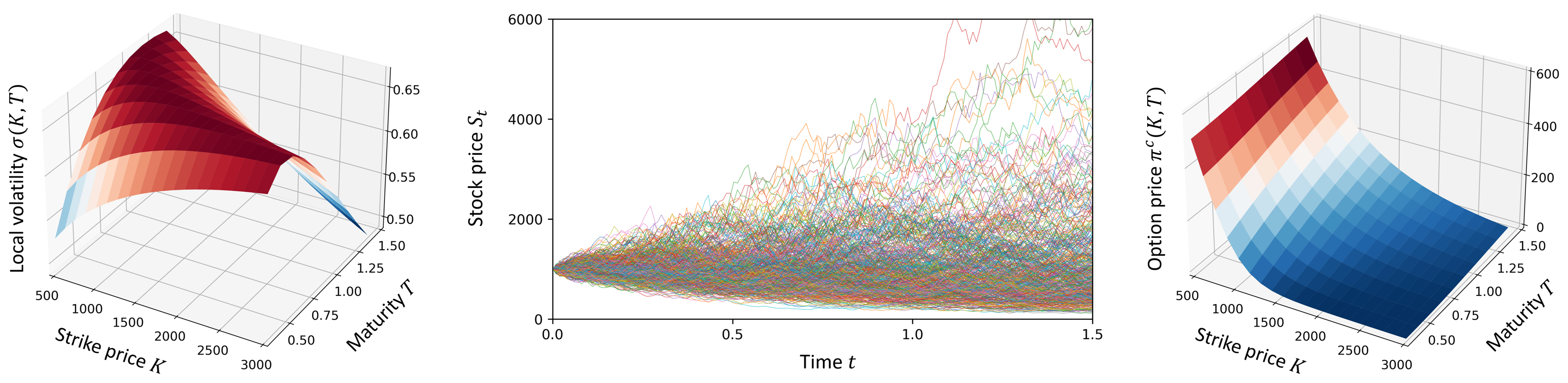
Figure 1: Left: exact local volatility surface, cf. Eq. (30); middle: simulated price trajectories by solving the local volatility model. cf. Eq. (1); and right: generated call option price using Monte Carlo simulation of Eq. (3a) with $10^{6}$ sampled price trajectories. The local volatility and the option price surfaces are visualized on an evenly spaced $10\times 20$ grids and, for a better visualization, only the first $1024$ price trajectories are shown in the middle pane.

Without loss of generality, we take a constant $r=0.04$ and

$$\sigma(x,t)=0.3+ye^{-y}\quad\mbox{with}\quad y=(t+0.1)\sqrt{x+0.1}.$$ (30)

The price trajectories are obtained by simulating Eq. (1) for $10^{6}$ times from a single initial condition $S_{0}=1,000$ for the period $t=[0,1.5]$ and with a time step $\mathrm{d}t=0.01$. To begin with, we price European call options on a mesh grid consisting of evenly spaced $10$ points for the $[0.3,1.5]$ $T$-period and $20$ points in the $[500,3000]$ $K$-interval, respectively. That is, the dataset consists of $10\times 20$ option prices quoted at the corresponding strike-maturity pairs, leading to the triplet $(\pi^{c}_{i},K_{i},T_{i})$ with $i=1,...,200$. The exact local volatility surface, the simulated price trajectories by numerically integrating the local volatility model, and the synthetic call option price surface are visualized in Figure 1.

The triplet of the synthetic call options are rescaled for training, cf. Eq. (10). As soon as $\boldsymbol{\theta}_{c}$ and $\boldsymbol{\theta}_{\eta}$ are determined, the parameterized option price and the calibrated local volatility are recovered by calling Eqs. (18) and (29), respectively. Thereafter, we substitute the calibrated neural local volatility into Eq. (1), forming a neural local volatility model, whose solution, in turn, gives the synthetic stock prices, from which the option price can then be recovered using Monte Carlo estimates of Eq. (3a), completing a control loop for model assessment. The calibrated local volatility, the simulated price trajectory by numerically integrating the neural local volatility model with a pre-sampled sequence of $B_{t}$, and the relative errors of calibrated local volatility with respect to the exact expression (30) are shown in Figure 2. For $\lambda=0$, the parameterized option price is not regularized by a priori physics information encoded in Dupire’s equation, reducing the self-consistent calibration of local volatility to a one-way approach. In both cases, the parameterized option price are regularized by the arbitrage-free conditions as in previous works [ATV20, CCD20, CCC⁺21], yet exploiting self-consistency by the inclusion of $L_{\text{dup}}$ a regularizer improves significantly the calibrated local volatility surface.

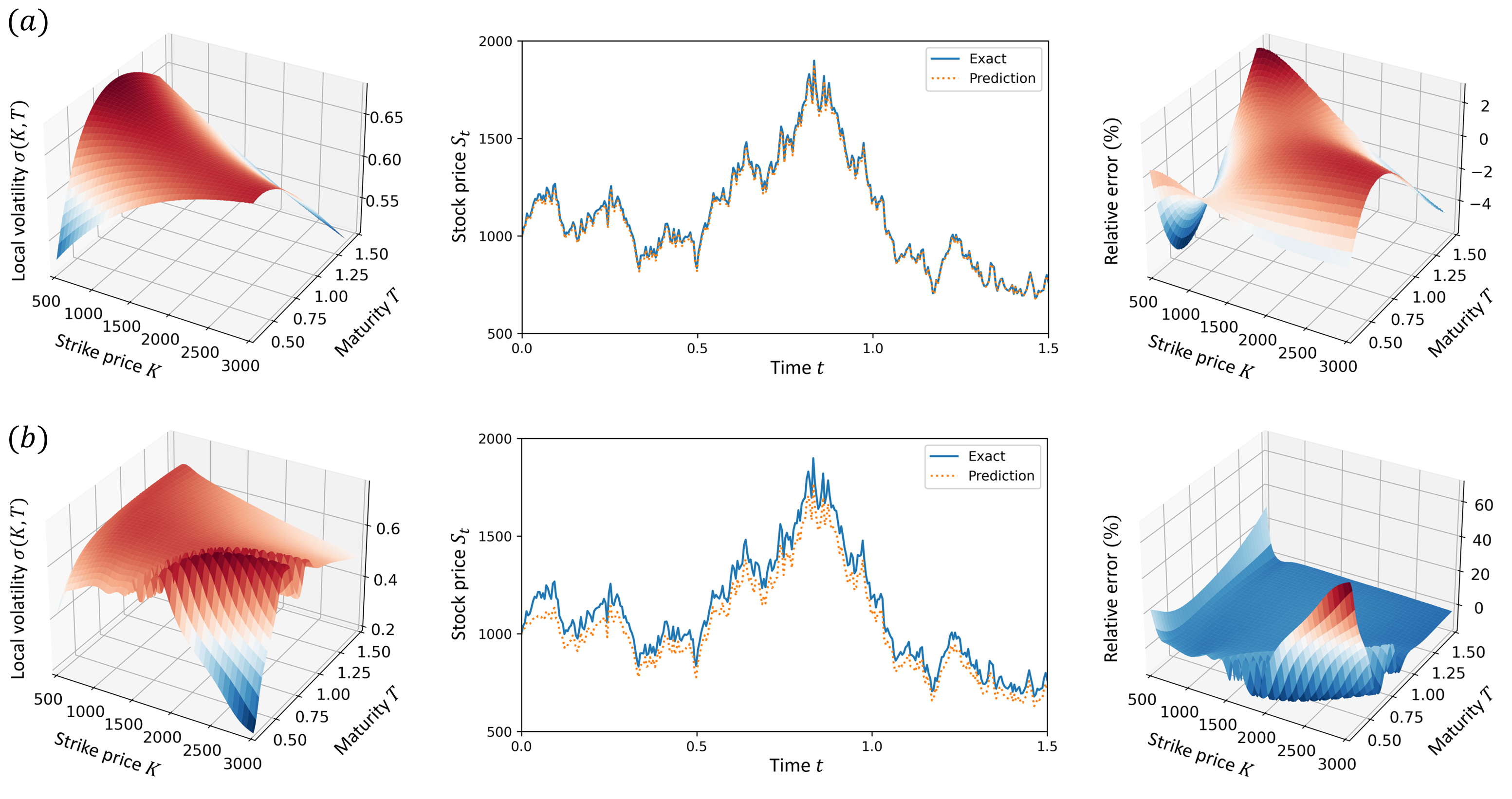
Figure 2: Visualization of calibrated neural local volatility (left), simulated price trajectory with a pre-sampled standard Brownian motion $B_{t}$ (middle), and the relative error of the calibrated local volatility with respect to the exact expression (30) $(a)$ with ($\lambda_{\text{dup}}=1$); and $(b)$ without ($\lambda_{\text{dup}}=0$) the inclusion of $L_{\text{dup}}$ as regularizer. The models shown in are trained on a dataset consists of $10\times 20$ option prices, while the visualization and relative errors are computed on a different test grid with linearly spaced $256\times 256$ collocation points.

To explore the small data limit of the proposed method, we present in Figure 3 the calibrated local volatility surface from a scarce dataset consisting of $3\times 6$ option prices quoted on a linearly spaced grid $(K,T)\in[500,3000]\times[0.3,1.5]$. It is observed that the use of self-consistency effectively compensates the lack of data, validating the proposed method in the small data limit. Indeed, neural networks are essentially nonlinear functions. Given discrete pairs of inputs and outputs, such a mapping function is not uniquely determined. To ensure that the obtained neural networks can be generalized, one needs to go through the entire domain of definition of neural networks, calling for big data. Alternatively, incorporating a priori physics information, completely or partially known, into the learning scheme can regularize neural networks at places where there is no data, allowing one to be benefit from recent advance in deep learning without bid data.

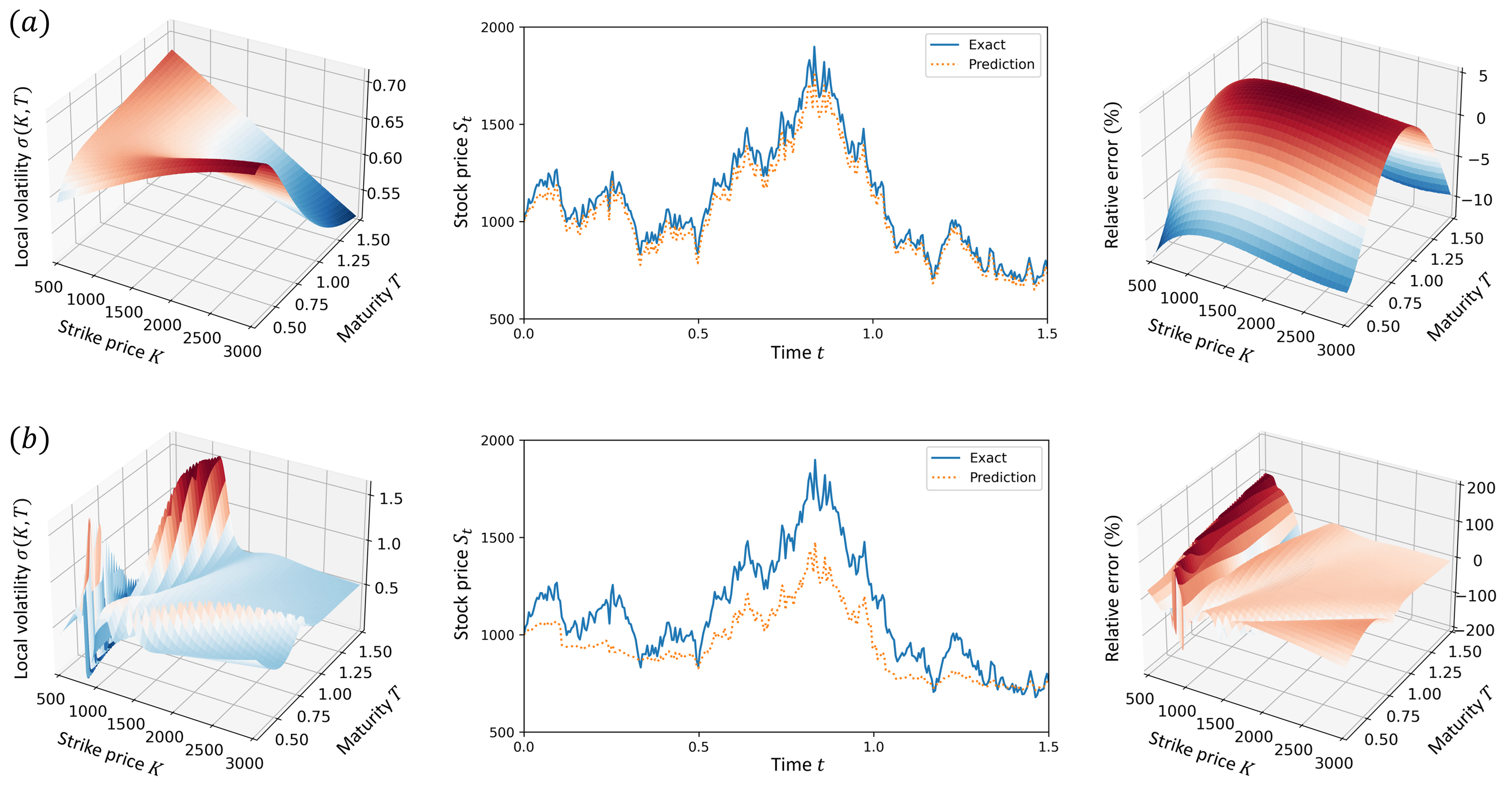
Figure 3: Same as in Figure 2, but with the models trained on a scarce dataset consisting of $3\times 6$ option prices quoted on a linearly spaced grid $(K,T)\in[500,3000]\times[0.3,1.5]$.

To investigate the sensitivity of the proposed method with respect to $\lambda$, we consider a sequence of values in the range $\lambda=[0,4]$. We quantify the accuracy of our self-consistent method by the root mean squared error (RMSE) for the parameterized option price and the calibrated local volatility. Here, independent of the training dataset, RMSEs are computed on a different testing grid consisting of a linearly spaced $256\times 256$ collocation points in $[K,T]\in[500,3000]\times[0.3,1.5]$. We perform three independent runs for each case and the averaged results are summarized in Table 1. It is observed that, with increasing $\lambda$ from $0$, RMSEs for the calibrated volatility and the repriced option price first decrease then increase, indicative the existence of an optimal $\lambda$. The value of optimal $\lambda$ seems to be dependent on the size of dataset and its determination is out of the scope of this paper, hence left for future work. The decreased RMSEs for any reasonably chosen $\lambda\neq 0$ support the inclusion of $L_{\text{dup}}$ for regularizing the parameterized option price. With randomly initialized $\boldsymbol{\theta}_{\eta}$, the corresponding Dupire equation forms essentially a wrong a priori for the measured data. During the training, a joint minimization of $L_{\pi}$ with respect to $\boldsymbol{\theta}_{c}$ and of $L_{\text{dup}}$ with respect to $\boldsymbol{\theta}_{\eta}$ yields a self-consistent pair of parameterized option price that provides an optimized description for the measured data, initial and boundary conditions, arbitrage-free conditions, and the underlying Dupire’s equation; as well as the calibrated local volatility that matches, upon a physics-informed correction, the price dynamics of the observed data. Assigning a too small weight leads to unregularized parameterization, whereas a large $\lambda$ slows down the minimization, resulting in an increased calibration error with a fixed number of iterations.

Dataset	RMSEs	$\lambda$
		$0.0$	$0.5$	$1.0$	$1.5$	$2.0$
$3\times 6$	Option price	$10.53$	$2.27$	$1.95$	$1.62$	$1.76$
	Local volatility	$0.25$	$0.03$	$0.03$	$0.02$	$0.03$
	Reprice error	$64.54$	$1.84$	$1.88$	$1.81$	$1.71$
$10\times 20$	Option price	$1.07$	$1.76$	$0.94$	$1.10$	$1.22$
	Local volatility	$0.04$	$0.01$	$0.01$	$0.01$	$0.02$
	Reprice error	$5.99$	$1.23$	$1.16$	$1.08$	$1.34$

Table 1: Test of proposed self-consistent method on synthetic dataset.

4.2 Application to market data

4.2.1 European call options on DAX index

To perform a comparison with previous works [CCD20, Cré02], we take the daily dataset of DAX index European call options listed on the $7$-th, $8$-th, and $9$-th, August 2001. The spot prices for the underlying assets are $S_{0}=5752.51,5614.51,5512.28$, respectively, with $217$, $217$, and $218$ call options quoted at differential strike-maturity pairs. For simplicity, we take $r=0.04$ constant. The calibrated local volatility surfaces with and without the inclusion of $L_{\text{dup}}$ as regularizer are shown in Figure 4. It is observed that, comparing with the case $\lambda=0$, the inclusion of $L_{\text{dup}}$ suppresses the variation of the local volatility surfaces over successive days. However, to determine whether the variations that we observe in Figure 4 $(b)$ are linked with overfitting, we resort to the quantitative analysis below.

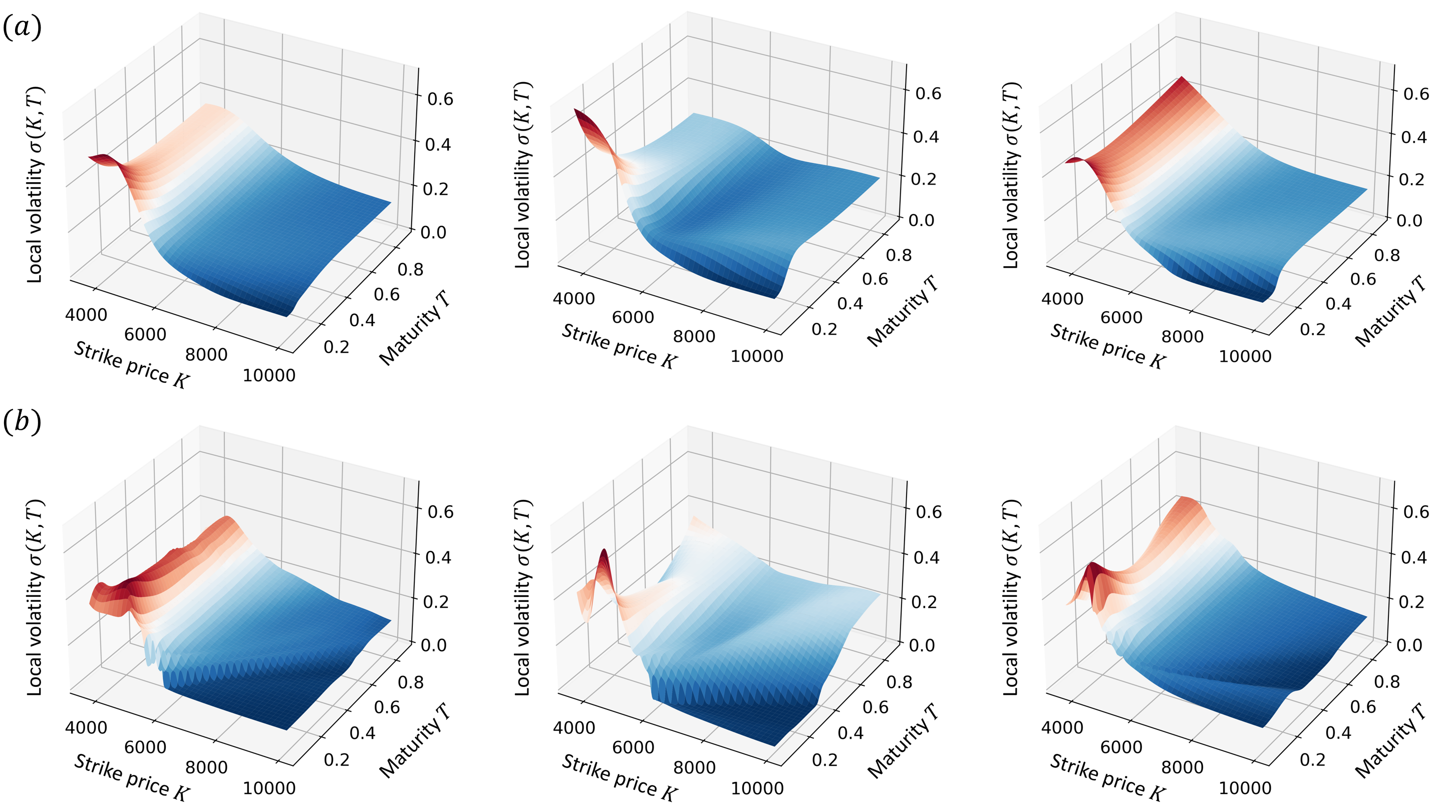
Figure 4: Visualization for the neural local volatility surface calibrated $(a)$ with ($\lambda_{\text{dup}}=1.0$); and $(b)$ without ($\lambda_{\text{dup}}=0.0$) the inclusion of the residue of Dupire’s equation as a regularizer. The obtained results are trained with DAX call option prices listed on $7$-th (left), $8$-th (middle), and $9$-th (right) August 2001.

As in [CCD20], we assess the calibrated local volatility by computing the reprice RMSEs and the results are summarized in Table 2. Note that our results shown are averaged over three independent runs. The unregularized calibration, i.e. $\lambda_{\text{dup}}=0$, leads to relatively large reprice RMSEs, evidencing that the observed variations of local volatility surface over successive days in Figure 4 are indeed due to overfitting. On the other hand, compared with previous works using Tikhonov regularization [Cré02] and with regularizer that impose positiveness and boundedness of the local volatility [CCD20], the inclusion of $L_{\text{dup}}$ as a regularizer reduces significantly the reprice RMSEs, leading to the best results. This, therefore, asserts quantitatively the effectiveness of the proposed self-consistent approach.

Reprice RMSE	Ours		Tikhonov	Price based neural network
	$\lambda=0$	$\lambda=1$
7 August 2001	9.44	2.85	5.42	10.18
8 August 2001	6.16	3.27	5.55	7.44
9 August 2001	8.93	2.67	4.60	8.18

Table 2: Comparison of reprice RMSEs with [Cré02], [CCD20] on DAX call options.

4.2.2 Put options on the SPX index

In our second application to the market data, we use the same dataset, i.e. SPX European put options listed on 18th May 2019, as in [CCC⁺21]. The put options are quoted on maturities $T\in[0.055,2.5]$ and with various strike prices $K\in[1150,4000]$. Spot price of the underlying is $S_{0}=2859.53$ and, for simplicity, we take $r=0.023$ constant. Following [CCC⁺21], the dataset is split into a training dataset and a testing dataset consisting of $1720$ and $1725$ market put option prices, enabling a comparison. The calibrated local volatility surfaces for the cases $\lambda=0$ and $\lambda=1$, as well as their relative difference are shown in Figure 5. It is observed that a numerical singularity developed around $K=3000$ for the case $\lambda=0$ is suppressed with the inclusion of $L_{\text{dup}}$ as a regularizer.

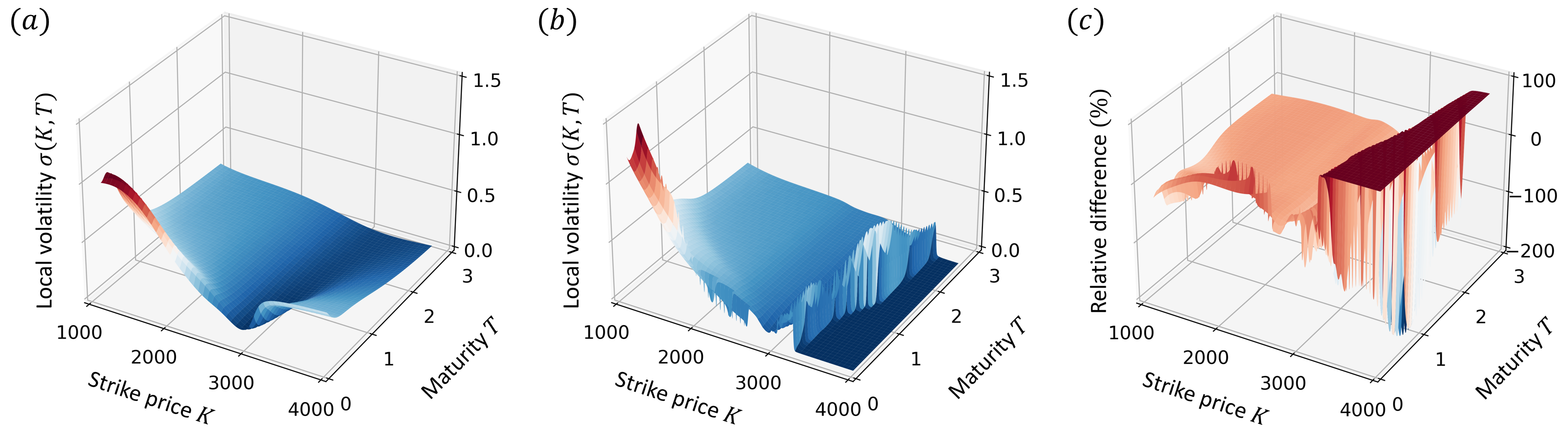
Figure 5: Visualization for the neural local volatility surface calibrated $(a)$ with ($\lambda=1$); $(b)$ without ($\lambda=0$) the inclusion of the residue of Dupire’s equation as a regularizer; and the relative difference of the local volatility surface obtained in $(b)$ computed with respect to that in $(a)$. The obtained results are trained with SPX call option prices listed on 18th May 2019. For better visualization, the relative difference in $(c)$ is truncated at $100\%$.

Next, on the testing dataset, we evaluate the interpolation and reprice RMSEs of the option prices with and without the inclusion of $L_{\text{dup}}$ as a regularizer, and then compare our results with published benchmarks obtained using various methods in Table 3. They are surface stochastic volatility inspired (SSVI) model, Gaussian process (GP), as well as implied volatility (IV) based and price based neural networks, see [CCC⁺21] for details. In Table 3, the RMSEs are evaluated on the testing grid and our results shown are averaged over three independent runs. With $\lambda=1$, our proposed method achieves the lowest reprice RMSEs on the testing dataset, confirming the significance of the proposed self-consistent approach. It is interesting to note that the Gaussian process, which achieves the lowest interpolation error among all methods, results in the highest reprice RMSEs. This can indicate that the market data of the put option prices contain significant amount of noises, which may be linked with the singular behavior as we observed in Figure 5$(b)$, leading eventually to the high reprice RMSEs in Table 3. Consequently, compared with that of $\lambda=0$, a simultaneous increase in interpolation RMSE and decrease in reprice RMSEs for the case $\lambda=1$ may imply a physics-informed correction to the market data via self-consistency.

RMSEs	Ours		SSVI	GP	Neural networks
	$\lambda=0$	$\lambda=1$			IV	Price
Interpolation	0.97	1.92	2.89	0.26	2.97	10.35
Reprice	5.24	3.26	22.83	74.02	4.99	11.76

Table 3: Comparison of interpolation and reprice RMSEs with [CCC⁺21] on SPX put options.

5 Discussion and conclusions

In this work, we introduce a deep learning method that yields the parameterized option price and the calibrated local volatility in a self-consistent manner. More specifically, we approximate both the option price and the local volatility using deep neural networks. Self-consistency is established through Dupire’s equation in the sense that the parameterized option price from the market data is required to be a solution to the underlying Dupire’s equation with the calibrated local volatility. Consequently, by exploiting self-consistency, one not only calibrates the local volatility surface from the market option prices, but also filters out noises in the data that violate Dupire’s equation with the calibrated local volatility, going beyond classical inverse problems with regularization.

The proposed method has been tested on both synthetic and market option prices. In all cases, the proposed self-consistent method results in a smooth surface for the calibrated local volatility, with the reprice RMSEs are lower than that obtained either by the canonical methods or the deep learning approaches [Cré02, AP05, CCD20, CCC⁺21]. Moreover, the reprice RMSEs are relatively insensitive to the regularization parameter $\lambda>0$, showing the robustness of our algorithm. Being continuous functions, the neural networks provide full surfaces for the parameterized option price and for the calibrated local volatility, at variance with discrete nodes using the canonical methods. However, by incorporating the residue of Dupire’s equation as a regularizer, one needs to solve a two-dimensional partial differential equation at each iteration, leading to increased computation time. This drawback, however, can be mitigated by distributing the training task on multiple GPUs.

Although the option price varies dramatically due to the price dynamics of the underlying assets, it is observed from Figure 4 that the variation local volatility surface over successive days remains small. Indeed, as the volatility measures the uncertainty of future price movement of the underlying assets, a large variation in the local volatility surface would imply a dramatic change in the market. Therefore, instead of starting from random initial parameters, initiating the training from converged solutions of the previous day can lead to a substantially reduction in computation time, cf. [WG21] for a case study. Alternatively, modeling the local volatility as a continuous function of time, namely $\sigma=\sigma(t,K,T)$, could be useful for investigating the temporal evolution of the local volatility surface. In this case, market option prices of successive days can be used to train, jointly, one local volatility model. Under an assumption that the temporal evolution of local volatility is characterized a deterministic dynamics, one may deduce the underlying ordinary differential equation for $\sigma(t,K,T)$ on a fixed grid $(K,T)$, enabling a propagation of the local volatility surface forward in time. The predicted local volatility surface could be useful for, e.g. risk management.

References

- [AP05] Y. Achdou and O. Pironneau. Computational Methods for Option Pricing. Society for Industrial and Applied Mathematics, 2005.
- [ATV20] D. Ackerer, N. Tagasovska, and T. Vatter. Deep smoothing of the implied volatility surface. In Proceedings of the 34th Conference on Neural Information Processing Systems (NeurIPS), pages 11552–11563, 2020.
- [Ben14] C. Bennett. Trading Volatility, Correlation, Term Structure and Skew. CreateSpace, 2014.
- [BPRS17] A. G. Baydin, B. A. Pearlmutter, A. A. Radul, and J. M. Siskind. Automatic differentiation in machine learning: a survey. Journal of Machine Learning Research, 18(1):5595–5637, 2017.
- [CCC+21] M. Chataigner, A. Cousin, S. Crépey, M. Dixon, and D. Gueye. Beyond surrogate modeling: Learning the local volatility via shape constraints. SIAM Journal on Financial Mathematics, 12(3):SC58–SC69, 2021.
- [CCD20] M. Chataigner, S. Crépey, and M. Dixon. Deep local volatility. Risks, 8(3):82, 2020.
- [Cré02] S. Crépey. Calibration of the local volatility in a trinomial tree using Tikhonov regularization. Inverse Problems, 19(1):91, 2002.
- [DK94] E. Derman and I. Kani. Riding on a smile. Risk, 7(2):139–145, 1994.
- [Dup94] B. Dupire. Pricing with a smile. Risk, 7(1):18–20, 1994.
- [GW98] A. N. Gorban and D. C. Wunsch. The general approximation theorem. In Proceedings of the International Joint Conference on Neural Networks, volume 2 of 1271-1274, 1998.
- [Hul03] J. C. Hull. Options futures and other derivatives. Pearson Education, 2003.
- [HZRS16] K. He, X. Zhang, S. Ren, and J. Sun. Deep residual learning for image recognition. In Proceedings of the IEEE conference on computer vision and pattern recognition, 2016.
- [IS15] S. Ioffe and C. Szegedy. Batch normalization: Accelerating deep network training by reducing internal covariate shift. In International conference on machine learning, pages 448–456, 2015.
- [Itk20] A. Itkin. Fitting Local Volatility. World Scientific, 2020.
- [KKL+21] G. E. Karniadakis, I. G. Kevrekidis, L. Lu, P. Perdikaris, S. Wang, and L. Yang. Physics- informed machine learning. Nature Reviews Physics, 3:422–440, 2021.
- [LJ18] H. Lin and S. Jegelka. Resnet with one-neuron hidden layers is a universal approximator. In Advances in Neural Information Processing Systems, page 6172–6181, 2018.
- [Pri22] N. Privault. Introduction to Stochastic Finance with Market Examples. Financial Mathematics Series. Chapman & Hall/CRC, second edition, 2022.
- [RMM+20] C. Rackauckas, Y. Ma, J. Martensen, C. Warner, K. Zubov, R. Supekar, D. Skinner, A. Ramadhan, and A. Edelman. Universal differential equations for scientific machine learning. Preprint arXiv:2001.04385, 2020.
- [RPK19] M. Raissi, P. Perdikaris, and G. E. Karniadakis. Physics-informed neural networks: A deep learning framework for solving forward and inverse problems involving nonlinear partial differential equations. Journal of Computational Physics, 378:686–707, 2019.
- [WG21] Z. Wang and C. Guet. Deep learning in physics: a study of dielectric quasi-cubic particles in a uniform electric field. IEEE Transactions on Emerging Topics in Computational Intelligence, 2021. , doi: 10.1109/TETCI.2021.3086237.
- [WG22] Z. Wang and C. Guet. Self-consistent learning of neural dynamical systems from noisy time series. IEEE Transactions on Emerging Topics in Computational Intelligence, Early Access:1–10, 2022.
- [WL17] D. A. Winkler and T. C. Le. Performance of deep and shallow neural networks, the universal approximation theorem, activity cliffs, and QSAR. Molecular Informatics, 36(1-2):1600118, 2017.