PDE-Based Optimal Strategy for Unconstrained Online Learning

Abstract

Unconstrained Online Linear Optimization (OLO) is a practical problem setting to study the training of machine learning models. Existing works proposed a number of potential-based algorithms, but in general the design of these potential functions relies heavily on guessing. To streamline this workflow, we present a framework that generates new potential functions by solving a Partial Differential Equation (PDE). Specifically, when losses are 1-Lipschitz, our framework produces a novel algorithm with anytime regret bound $C\sqrt{T}+\|{u}\|\sqrt{2T}[\sqrt{\log(1+\|{u}\|/C)}+2]$, where $C$ is a user-specified constant and $u$ is any comparator unknown and unbounded a priori. Such a bound attains an optimal loss-regret trade-off without the impractical doubling trick. Moreover, a matching lower bound shows that the leading order term, including the constant multiplier $\sqrt{2}$, is tight. To our knowledge, the proposed algorithm is the first to achieve such optimalities.

1 Introduction

Advances in online learning have brought deeper understanding and better algorithms to the training of machine learning models. Among all the problem settings therein, unconstrained online learning has received special attention since the parameter of the model is often unrestricted before seeing any data. Compared to conventional settings with a bounded domain, the unconstrained setting poses an additional challenge: starting from a bad initialization, how can an algorithm quickly find the optimal parameter that may be far-away? With the growing popularity of high-dimensional models, such an issue becomes increasingly important.

In this paper, we address this issue by studying a theoretical problem called unconstrained Online Linear Optimization (OLO). Given an unbounded domain $\mathbb{R}^{d}$, we need to design an algorithm such that in each round it makes a deterministic prediction $x_{t}\in\mathbb{R}^{d}$, observes a loss gradient $g_{t}\in\mathbb{R}^{d}$ and suffers a loss $\left\langle g_{t},x_{t}\right\rangle$, where $g_{t}$ is adversarial (can arbitrarily depend on $x_{1},\ldots,x_{t}$) and satisfies $\|{g_{t}}\|\leq 1$. The considered performance metric is the regret

$$\mathrm{Regret}_{T}(u)=\sum_{t=1}^{T}\left\langle g_{t},x_{t}\right\rangle-\sum_{t=1}^{T}\left\langle g_{t},u\right\rangle,$$

and the goal is to achieve low regret for all comparator $u\in\mathbb{R}^{d}$, time horizon $T\in\mathbb{N}_{+}$ and loss gradients $g_{1},\ldots,g_{T}$. Besides pursuing the optimal rate on $T$, we are also interested in the dependence of $\mathrm{Regret}_{T}(u)$ on $\|{u}\|$, as it captures how well the algorithm performs if the optimal fixed prediction (in hindsight) turns out to be far-away from the user’s prior guess (in this case, the origin).

Many algorithms for unconstrained OLO are based on the potential method. Given a potential function $V_{t}(\cdot)$, the key idea is to accumulate the history into a “sufficient statistic” $S_{t}=-\sum_{i=1}^{t-1}g_{i}$ and predict the gradient of $V_{t}(\cdot)$ at $S_{t}$, i.e., $x_{t}=\nabla V_{t}(S_{t})$. Through this procedure, designing new algorithms is converted into a more tangible task of finding good potentials. Specifically, with an arbitrary constant $C$, existing works (e.g., [35, 37, 34]) adopted the one-dimensional potential

$$V_{t}(S_{t})=\frac{C}{\sqrt{t}}\exp\left({\frac{S^{2}_{t}}{2t}}\right)$$ (1)

and its variants to achieve the regret bound

$$\mathrm{Regret}_{T}(u)\leq C+\|{u}\|O\left({\sqrt{T\log\frac{\|{u}\|\sqrt{T}}{C}}}\right).$$ (2)

Among all the achievable upper bounds with $\mathrm{Regret}_{T}(0)\leq C$, the order of $\|{u}\|$ and $T$ in (2) is optimal up to multiplicative constants. In practice, these algorithms have demonstrated promising performance with minimum hyperparameter tuning [40, 10].

Despite these strong results, there is still room for improvement though. Intuitively, requiring a constant $\mathrm{Regret}_{T}(0)$ all the time amounts to a strong belief that the initialization of the model is close to the optimal parameter, which somewhat contradicts the use of an unconstrained domain in the first place. Reflected in the regret bound, the RHS of (2) can be more generally viewed as a trade-off between the values of $\mathrm{Regret}_{T}(u)$ at small $\|{u}\|$ and large $\|{u}\|$: if the cumulative loss $\mathrm{Regret}_{T}(0)$ is allowed to increase with $T$, then one may obtain lower regret with respect to far-away comparators. This will be favorable in high-dimensional problems, as good initializations become harder to obtain.

The question now becomes, what is the optimal loss-regret trade-off, and how to efficiently achieve it? As a first attempt, one could assume a known time horizon $T$, set $C=\sqrt{T}$ in (2) and obtain [35]

$$\mathrm{Regret}_{T}(u)\leq\sqrt{T}+\|{u}\|O\left({\sqrt{T\log\|{u}\|}}\right).$$ (3)

With respect to $T$ alone, $R_{T}(u)=O(\sqrt{T})$. Since it matches the standard minimax lower bound for constrained OLO, we consider this loss-regret trade-off as optimal. The real challenge is an anytime bound - existing arguments rely on a doubling trick [45], which not only is notoriously impractical, but also leads to an extra multiplying constant with unclear optimality. Perhaps due to this reason, regret bounds like (3) have received a lot less attention than (2), despite its theoretical advantages.

The present work aims at a practical and optimal approach towards an anytime bound in the form of (3) - this requires a significant departure from existing techniques. Specifically, we will go back one step and rethink the design of potential functions in unconstrained OLO. The classical workflow is based on heuristic guessing, which is challenging when the suitable potential is not an elementary function (e.g., involving complicated integrals or series). Our goal is to propose a systematic approach for this task, which reduces the amount of guessing and allows us to handle more complicated potentials. Eventually, as a byproduct, our framework produces a new algorithm that efficiently achieves the optimal loss-regret trade-off.

1.1 Result and contribution

As motivated above, our contributions are twofold.

• We propose a framework that uses solutions of a specific Partial Differential Equation (PDE) as potential functions for unconstrained OLO. To this end, we characterize minimax optimal potentials via a backward recursion, and our PDE naturally arises in its continuous-time limit. Solutions of this PDE approximately solve the discrete-time recursion. Therefore, one may search for suitable potentials within such solutions and their variants, which is a more structured procedure than direct guessing.

• Using our framework, we design a one-dimensional potential which is not elementary and hard to guess without the help of a PDE. The induced algorithm guarantees

  $$\mathrm{Regret}_{T}(u)\leq C\sqrt{T}+\left\|{u}\right\|\sqrt{2T}\left[{\sqrt{\log\left({1+\frac{\left\|{u}\right\|}{\sqrt{2}C}}\right)}+2}\right].$$

  Our bound achieves an optimal loss-regret trade-off (3) without the doubling trick. Moreover, by constructing a matching lower bound, we further show that the leading order term, including the constant multiplier $\sqrt{2}$, is tight. To our knowledge, the proposed algorithm is the first to achieve such optimalities. The obtained theoretical benefits are validated by experiments.

1.2 Related work

Unconstrained OLO

Unconstrained convex optimization has been extensively studied in both the offline and online settings. Typically, strong guarantees can be obtained assuming certain curvature on the loss function. Without curvature, the problem becomes harder but more practical for large scale applications (e.g., training machine learning models), as gradients become the only available feedback.

For unconstrained OLO, if the optimal learning rate in hindsight is known a priori, Online Gradient Descent (OGD) [49] guarantees $O(\|{u}\|\sqrt{T})$ regret with respect to the optimal comparator $u$. Without that prior knowledge, the regret bound downgrades to $O(\|{u}\|^{2}\sqrt{T})$. A line of works on parameter-free algorithms aim at achieving $\tilde{O}(\|{u}\|\sqrt{T})$ regret in the latter setting. Specifically, McMahan and Steeter [36] proposed the first parameter-free algorithm with $O(\|{u}\|\sqrt{T}\log(\|{u}\|T))$ regret, which was later improved to $O(\|{u}\|\sqrt{T\log(\|{u}\|T)})$ by a potential-based algorithm [35]; this is the optimal rate [36, 38, 39] given the constraint $\mathrm{Regret}_{T}(0)\leq\textrm{constant}$. More recently, the analysis was streamlined in [37, 11] through a coin-betting game, and in [21] through the Burkholder method. The obtained algorithms find applications in differential privacy [24, 46], combining optimizers [14, 15, 47] and training neural networks [40].

Among all these results, a shared limitation is the focus on $\mathrm{Regret}_{T}(0)\leq\textrm{constant}$. Other forms of loss-regret trade-offs are less explored, both theoretically and practically. Moreover, the optimality of leading constants has not been considered.

Differential equations for online learning

Recently, applying differential equations in online learning has received growing interests. The first idea was proposed by Kapralov and Panigrahy [29], where a potential function for Learning with Expert Advice (LEA) [31] was designed by solving an Ordinary Differential Equation (ODE). As a key benefit, the obtained regret bound achieves a trade-off with respect to different individual experts. The proposed techniques were later applied to the discounted setting [2] and the movement-constrained setting [20]. Interestingly, our prior work [47] used the coin-betting approach to achieve a similar goal as [20], suggesting intriguing connections between differential equations and parameter-free online learning.

An improved approach uses PDEs (rather than ODEs) to generate time-dependent potential functions. Still considering the LEA problem, such works aim at the optimal regret bound nonasymptotic in the number of experts. Zhu [48] first derived a PDE to characterize the continuous-time limit of LEA, whose arguments were streamlined by Drenska and Kohn [19]. Exact solutions were obtained in special cases [5, 6, 19], and more generally, algorithms based on approximate solutions were designed in [43, 26, 27]. Follow-up works considered history-dependent experts [18, 16] and malicious experts [9, 7]. Furthermore, Harvey et al. [23] extended this idea to the anytime setting with two experts, using a different, stochastic derivation of the continuous-time PDE.

Our use of PDE in unconstrained OLO is inspired by these works on LEA. Notably, we emphasize two differences.

• Existing works considered settings that enforce a unique solution to the PDE, by requiring a fixed time horizon (e.g., [48, 19, 26]) or imposing boundary conditions [23]. In contrast, we directly consider a class of solutions which are generally not comparable to each other.

• In LEA, the goal of the PDE approach is to achieve the optimal uniform regret (with respect to all experts). In contrast, we use a PDE to achieve performance trade-offs in adaptive online learning. Trade-offs among experts have been studied using ODEs (e.g., [29]). However, we focus on the anytime setting, and the trade-off in unconstrained OLO is with respect to all comparators in $\mathbb{R}^{d}$, which is more challenging.

1.3 Notation

Let $\|{\cdot}\|$ be the Euclidean norm, and let $\mathsf{B}^{d}$ be the unit $d$-dimensional Euclidean norm ball. For a twice differentiable function $V(t,S)$ where $t$ represents time and $S$ represents a spatial variable, let $\nabla_{t}V$, $\nabla_{tt}V$, $\nabla_{S}V$ and $\nabla_{SS}V$ be the first and second order partial derivatives. $\lambda_{\max}(\cdot)$ is the largest eigenvalue of a real symmetric matrix. For a function $f$, let $f^{*}$ be its Fenchel conjugate. For two integers $a\leq b$, $[a:b]$ is the set of all integers $c$ such that $a\leq c\leq b$; the brackets are removed when on the subscript, denoting a finite sequence with indices in $[a:b]$. Finally, $\log$ denotes natural logarithm when the base is omitted.

2 OLO, betting and limiting PDE

Our approach critically relies on a continuous-time view of the discrete-time unconstrained OLO problem. It consists of three steps, detailed in the following three subsections. First, we convert OLO to a coin-betting problem - the latter is easier from a technical perspective, due to the absence of comparators.

2.1 Unconstrained coin-betting and duality

Unconstrained coin-betting is a two-person zero-sum game, with $\mathcal{X}=\mathbb{R}^{d}$ and $\mathcal{C}=\mathsf{B}^{d}$ being the action space of the player and the adversary respectively. The player’s policy $\bm{p}$ contains an initial bet $x_{1}\in\mathcal{X}$ and a collection of functions $\{p_{2},p_{3},\ldots\}$, with $p_{t}:\mathcal{C}^{t-1}\rightarrow\mathcal{X}$. Similarly, the adversary’s policy $\bm{a}$ is defined as a collection of functions $\{a_{1},a_{2},\ldots\}$, with $a_{t}:\mathcal{X}^{t}\rightarrow\mathcal{C}$. Analogous to our setting of unconstrained OLO, randomized betting strategies are not considered.

Fixing policies $\bm{p}$ and $\bm{a}$ on both sides, the game runs as follows. In the $t$-th round, the player makes a bet $x_{t}=p_{t}(c_{1:t-1})$ based on past coin outcomes. Then, the adversary decides a new coin $c_{t}=a_{t}(x_{1:t})$, reveals it to the player, and the player gains $\left\langle c_{t},x_{t}\right\rangle$ amount of money (effectively, the player loses money if $\left\langle c_{t},x_{t}\right\rangle$ is negative). The performance metric for the player is the total gained wealth

$$\mathrm{Wealth}_{T}=\sum_{t=1}^{T}\left\langle c_{t},x_{t}\right\rangle,$$

where $T$ is not pre-specified. In other words, the player aims to ensure an anytime wealth lower bound against all possible adversaries.

Research on adversarial betting has a long history, dating back at least to [12] - Cover studied the setting with a fixed and known time horizon, where all achievable lower bounds can be characterized via dynamic programming. Our anytime setting is more involved, but due to a classical dual relation [35], solving it is equivalent to solving the unconstrained OLO problem we ultimately care about: one can construct a unique OLO algorithm (Algorithm 1) from any coin-betting algorithm $\mathcal{A}$, and characterize its performance through Lemma 2.1. Consequently, the rest of the paper will focus on solving the betting problem in a principled way.

Algorithm 1 From coin-betting to OLO.

0:  An algorithm $\mathcal{A}$ for unconstrained coin-betting.

1:  for $t=1,2,\ldots$ do

2:     Query $\mathcal{A}$ for its $t$-th bet $x_{t}$ and predict it exactly in OLO.

3:     Observe loss gradient $g_{t}$ and suffer $\left\langle g_{t},x_{t}\right\rangle$.

4:     Let $c_{t}=-g_{t}$ and send it to $\mathcal{A}$ as the $t$-th coin outcome.

5:  end for

Lemma 2.1 (Theorem 9.6 of [39]).

Let $\Psi$ be any proper, closed and convex function. For all $T\in\mathbb{N}_{+}$, the following two statements are equivalent:

1. The unconstrained coin-betting algorithm $\mathcal{A}$ guarantees $\mathrm{Wealth}_{T}\geq\Psi\left({\sum_{t=1}^{T}c_{t}}\right)$ against any adversary.

2. The unconstrained OLO algorithm constructed from $\mathcal{A}$ guarantees $\mathrm{Regret}_{T}(u)\leq\Psi^{*}(u)$ for all $u\in\mathbb{R}^{d}$, against any adversarial loss sequence. ($\Psi^{*}$ is the Fenchel conjugate of $\Psi$.)

Before proceeding, we note that the above unconstrained coin-betting game strictly generalizes the well-known existing one for unconstrained OLO analysis [35, 37]. The latter assigns an initial wealth $C$ to the player, and the player’s betting amount $\left|{x_{t}}\right|$ should be less than the total wealth it possesses at the beginning of the $t$-th round. A budget constraint of this form faithfully models many real-world investment problems, but since our ultimate goal is online learning rather than any particular financial application, such a constraint is not necessary for our purpose. In fact, relaxing it gives us greater flexibility to achieve general forms of regret trade-offs beyond (2). Intuitively speaking, the player in our setting can make decisions solely based on the perceived risk-gain trade-off, without being constrained by its budget.

2.2 Minimax coin-betting

For the second step of our derivation, we will characterize the unconstrained coin-betting game from a minimax perspective. Rather than the value of the game, we consider a refined quantity called value function.

Definition 2.1 (Value function).

$V:\mathbb{N}\times\mathbb{R}^{d}\rightarrow\mathbb{R}$ is a value function of the unconstrained coin-betting game if

1. $V(0,0)=0$.

2. For all $t\in\mathbb{N}$, $V(t,\cdot)$ is continuous on $\mathbb{R}^{d}$.

3. For all $t\in\mathbb{N}$ and $S\in t\cdot\mathcal{C}$,

   $$V(t,S)=\min_{x\in\mathcal{X}}\max_{c\in\mathcal{C}}\left[{V(t+1,S+c)-\left\langle c,x\right\rangle}\right].$$ (4)

The recursive relation in Definition 2.1 is reminiscent of the conditional value function previously studied in online learning [44, 32, 19] and minimax dynamic programming [4]. The key difference is that we care about anytime performance, therefore a terminal condition to initiate the backward recursion (4) is missing. Rather than the value-to-go, we model the value-so-far. This largely complicates the analysis, as the solution of (4) is not unique (e.g., $V(t,S)=\textrm{constant}\cdot S$). In general, similar to the concept of Pareto optimality, different value functions are not comparable as they represent different trade-offs on the shape of the wealth lower bound (ultimately, the associated regret upper bound due to Lemma 2.1).

On the bright side, any value function can lead to a pair of player-adversary strategies with tight wealth lower and upper bounds. Given a good value function (or more generally, its approximation), a good betting algorithm can be naturally induced. The proof is deferred to Appendix A.1.

Lemma 2.2.

Given any value function $V$ satisfying Definition 2.1,

1. We can construct a player policy $\bm{p}^{*}$ such that for all $\bm{a}$ and $T\in\mathbb{N}_{+}$,

   $$\mathrm{Wealth}_{T}\geq V\left({T,\sum_{t=1}^{T}c_{t}}\right).$$

   In addition, for all $t$, the player’s bet $p^{*}_{t}(c_{1:t-1})$ depends on the past coins only through their sum $\sum_{i=1}^{t-1}c_{i}$.

2. We can construct an adversary policy $\bm{a}^{*}$ such that for all $\bm{p}$ and $T\in\mathbb{N}_{+}$,

   $$\mathrm{Wealth}_{T}\leq V\left({T,\sum_{t=1}^{T}c_{t}}\right).$$

To proceed, let us further define the unit time as the time interval between consecutive rounds in the coin betting game, and assign it to 1. In this way, the game can be analyzed on the real time axis $t\in\mathbb{R}_{+}$.

2.3 The scaled game and limiting PDE

Intuitively, solving the backward recursion (4) is difficult due to its discrete formulation. If we adopt a finer discretization on the time axis, then the recursion becomes “smoother” which is easier to describe using continuous-time analysis. To this end, let us introduce a scaled coin-betting game.

Definition 2.2 (Scaled game).

Given $\varepsilon>0$, the $\varepsilon$-scaled game is the unconstrained coin-betting game with unit time $\varepsilon^{2}$ and adversary action space $\varepsilon\cdot\mathcal{C}$. That is, actions are taken every $\varepsilon^{2}$ original unit time, and the adversary chooses the coin outcomes in a scaled set $\varepsilon\cdot\mathcal{C}$ instead of $\mathcal{C}$.

Similar to Definition 2.1, we can define $\varepsilon$-scaled value functions $V_{\varepsilon}$ on the scaled game. Moreover, we extend its domain and assume it is twice-differentiable on $\mathbb{R}_{>0}\times\mathbb{R}^{d}$. The backward recursion on $V_{\varepsilon}$ becomes

$$V_{\varepsilon}(t,S)=\min_{x\in\mathcal{X}}\max_{c\in\mathcal{C}}\left[{V_{\varepsilon}(t+\varepsilon^{2},S+\varepsilon c)-\left\langle\varepsilon c,x\right\rangle}\right].$$

Similar to [48, 19], we take a Taylor approximation on the RHS,

$$V_{\varepsilon}(t+\varepsilon^{2},S+\varepsilon c)=V_{\varepsilon}(t,S)+\varepsilon^{2}\nabla_{t}V_{\varepsilon}(t,S)+\varepsilon\left\langle c,\nabla_{S}V_{\varepsilon}(t,S)\right\rangle+\frac{\varepsilon^{2}}{2}\left\langle\nabla_{SS}V_{\varepsilon}(t,S)\cdot c,c\right\rangle+o(\varepsilon^{2}),$$

which leads to

$$0=\min_{x\in\mathcal{X}}\max_{c\in\mathcal{C}}\big{[}\left\langle c,\nabla_{S}V_{\varepsilon}(t,S)-x\right\rangle+\varepsilon\nabla_{t}V_{\varepsilon}(t,S)+\frac{\varepsilon}{2}\left\langle\nabla_{SS}V_{\varepsilon}(t,S)\cdot c,c\right\rangle+o(\varepsilon)\big{]}.$$

As $\varepsilon$ approaches $0$, the dominant term on the RHS is $\min_{x\in\mathcal{X}}\max_{c\in\mathcal{C}}\left\langle c,\nabla_{S}V_{\varepsilon}(t,S)-x\right\rangle$, therefore the outer minimizing argument should be $x=\nabla_{S}V_{\varepsilon}(t,S)$. Along this argument, taking $\varepsilon\rightarrow 0$ and plugging in $\mathcal{C}=\mathsf{B}^{d}$ (i.e., the unit $d$-dimensional Euclidean norm ball), we obtain a second order nonlinear PDE for a limiting value function.

Definition 2.3 (Limiting value function).

A function $\bar{V}:\mathbb{R}_{>0}\times\mathbb{R}^{d}\rightarrow\mathbb{R}$ is a limiting value function of the unconstrained coin-betting game if

$$\nabla_{t}\bar{V}=-\frac{1}{2}\max\{\lambda_{\max}(\nabla_{SS}\bar{V}),0\}.$$ (5)

The PDE (5) can be regarded as a continuous-time approximation of the backward recursion (4), and solving it, while still challenging, is more tractable than handling the discrete-time recursion itself. Given solutions of this PDE, one may invoke a perturbed analysis of Lemma 2.2 and obtain corresponding wealth lower bounds.

3 One-dimensional analysis

To demonstrate the power of the PDE framework, let us focus on the one-dimensional convex case where the nonlinear PDE (5) becomes linear. Despite this restriction, our approach can still handle the general $d$-dimensional unconstrained OLO problem due to a standard extension technique [11] reviewed in Appendix C.

For now, let us assume $d=1$. To further comply with the duality lemma (Lemma 2.1), we will consider $\bar{V}$ that are convex with respect to the second argument. Then, the PDE (5) reduces to the one-dimensional backward heat equation

$$\nabla_{t}\bar{V}=-\frac{1}{2}\nabla_{SS}\bar{V}.$$ (6)

Such a linear PDE has received considerable interest from the maths community [33, 41], since its initial value problem has an intriguing ill-posed issue. Interestingly, an insightful work by Harvey et al. [23] showed that the backward heat equation gives rise to an optimal two-expert LEA algorithm - the proposed techniques will be useful in our analysis as well. Our key observations are twofold:

• The PDE framework recovers both the OGD potential and the existing parameter-free potential (1), thus appears to be a very general approach for unconstrained OLO.

• The optimal potential that Harvey et al. adopted for two-expert LEA is also strong for adaptive online learning, resulting in an optimal unconstrained OLO algorithm in high-dimensions.

3.1 PDE-based policy class

Motivated by the classical parameter-free potential (1), let us consider the ansatz

$$\bar{V}(t,S)=t^{\alpha}g\left({c\cdot t^{\beta}S}\right),$$ (7)

where $\alpha$, $\beta$ and $c$ are constants, and $g:\mathbb{R}\rightarrow\mathbb{R}$ is a one-dimensional function to be determined. For simplicity we omit shifting on $S$, $t$ and the function value. In other words, once we find appropriate $(\alpha,\beta,c)$ and $g$, we immediately obtain a more general solution

$$\bar{V}(t,S)=C_{0}+(t+\tau)^{\alpha}g\left({c\cdot t^{\beta}(S+S_{0})}\right),$$

with shifting constants $C_{0}$, $\tau$ and $S_{0}$. Moreover, any linear combination of two solutions is also a solution, allowing the user to interpolate their induced behavior.

Plugging in (7) and letting $z=c\cdot t^{\beta}S$, the PDE (6) reduces to a second order linear ODE for the function $g$:

$$c^{2}t^{2\beta+1}g^{\prime\prime}(z)+2\beta zg^{\prime}(z)+2\alpha g(z)=0.$$

Letting $\beta=-1/2$ and $c=1/\sqrt{2}$, it becomes the standard Hermite type

$$g^{\prime\prime}(z)-2zg^{\prime}(z)+4\alpha g(z)=0,$$ (8)

whose general solutions can be expressed in power series [3, Chapter 7]. By varying the parameter $\alpha$, we obtain a rich class of limiting value functions $\bar{V}$.

To construct coin-betting policies, our key idea is to use $\bar{V}$ as a surrogate for the actual value function $V$ (Definition 2.1) and apply the same argument as in Lemma 2.2. Specifically, the adversary should pick the coin outcome that maximizes the RHS of the backward recursion (4), which is

$$c_{t}\in\operatorname*{arg\,max}_{c\in\mathcal{C}}\left[{\bar{V}\left({t,\sum_{i=1}^{t-1}c_{i}+c}\right)-\left\langle c,x_{t}\right\rangle}\right].$$ (9)

Since $\bar{V}$ is convex and $\mathcal{C}=[-1,1]$, the adversary can simply focus on the boundary coins $\{-1,1\}$, leading to the adversary policy presented in Algorithm 2.

Algorithm 2 PDE-based adversary policy.

0:  A limiting value function $\bar{V}$ for 1d unconstrained coin-betting.

1:  for $t=1,2,\ldots$ do

2:     Receive the player’s bet $x_{t}$ and choose the coin outcome as

$$c_{t}\in\operatorname*{arg\,max}_{c\in\{-1,1\}}\left[{\bar{V}\left({t,\sum_{i=1}^{t-1}c_{i}+c}\right)-\left\langle c,x_{t}\right\rangle}\right].$$ (10)

3:  end for

As for the player, the optimal bet is the one that minimizes the objective function in (9), which is equivalent to the discrete derivative shown in Algorithm 3. Intuitively, the discrete derivative serves as an approximation of the standard derivative in classical potential methods. Therefore, Algorithm 3 essentially has a potential-based structure, with the potential function $\bar{V}$ generated from a PDE. Alternatively, Algorithm 3 can be interpreted as a discrete approximation of Follow the Regularized Leader (FTRL) [1] whose regularizer is the Fenchel conjugate of $\bar{V}(t,\cdot)$. The equivalence of potential functions and regularizers has been discussed in [39, Section 7.3].

Algorithm 3 PDE-based player policy.

0:  A limiting value function $\bar{V}$ for 1d unconstrained coin-betting.

1:  for $t=1,2,\ldots$ do

2:     Choose the bet

$$x_{t}=\frac{1}{2}\left[{\bar{V}\left({t,\sum_{i=1}^{t-1}c_{i}+1}\right)-\bar{V}\left({t,\sum_{i=1}^{t-1}c_{i}-1}\right)}\right].$$ (11)

3:     Observe the coin outcome $c_{t}$ and store it.

4:  end for

3.2 Example

Before any technical analysis, let us demonstrate the generality of this framework through a few examples. We show how classical algorithms can be derived from this framework, and more importantly, we present a potential function which permits an optimal loss-regret trade-off. For any $\alpha$, let $\bar{V}_{\alpha}$ be a limiting value function obtained from (8). Let $C>0$ be any positive scaling constant.

Warm up: $\alpha=1$.

The Hermite ODE (8) has a solution $g(z)=C(2z^{2}-1)$, resulting in $\bar{V}_{1}(t,S)=C(S^{2}-t)$. Accordingly, Algorithm 3 bets $x_{t}=2C\sum_{i=1}^{t-1}c_{i}=x_{t-1}+2Cc_{t-1}$, which is equivalent to Online Gradient Descent (OGD) with learning rate $2C$. Notably, $\bar{V}_{1}$ also satisfies Definition 2.1; that is, $\bar{V}_{1}$ is not only a limiting value function, but also a value function for the discrete-time game. Therefore, both Algorithm 2 and Algorithm 3 can be directly analyzed through Lemma 2.2, as shown in Appendix B.1.

Recovering existing potentials: $\alpha=-1/2$.

The Hermite ODE can be solved by $g(z)=C\exp(z^{2})$, resulting in $\bar{V}_{-1/2}(t,S)=C\cdot t^{-1/2}\exp[S^{2}/(2t)]$. Such a potential recovers the existing popular choice (1), and its time shifted version $C\cdot(t+\tau)^{-1/2}\exp[S^{2}/(2(t+\tau))]$ naturally recovers the shifted potential [37] with minimum effort. Different from the previous example, $\bar{V}_{-1/2}$ does not satisfy Definition 2.1. Therefore, we should characterize its approximation error on the backward recursion (4) in order to quantify the performance of the induced player policy. This procedure will be demonstrated in the next subsection.

A new potential: $\alpha=1/2$.

The two linearly independent solutions of the Hermite ODE are both useful. First, $g(z)=\sqrt{2}Cz$ and $\bar{V}(t,S)=CS$. Such a potential leads to betting a fixed amount in coin-betting and shifting the coordinate system in unconstrained OLO. The idea is simple, and it will be applied in our experiments. For now, let us focus on the other solution which is more interesting.

$$g(z)=C\left[{2z\cdot\int_{0}^{z}\exp(x^{2})dx-\exp(z^{2})}\right],$$

and the corresponding potential is

$$\bar{V}_{1/2}(t,S)=C\sqrt{t}\left[{2\int_{0}^{\frac{S}{\sqrt{2t}}}\left({\int_{0}^{u}\exp(x^{2})dx}\right)du-1}\right].$$ (12)

Notably, as shown in Appendix B.3, $\nabla_{SS}\bar{V}_{1/2}(t,S)=\bar{V}_{-1/2}(t,S)$, suggesting possible deeper connections to the existing parameter-free algorithms. Harvey et al. [23] constructed a two-expert LEA algorithm from $\bar{V}_{1/2}$, which achieves the optimal uniform regret. As for unconstrained OLO, we will show that using $\bar{V}_{1/2}$ in Algorithm 3 leads to superior performance compared to $\bar{V}_{-1/2}$, both in theory and in practice. Without the help of a PDE, such a potential has not been discovered in adaptive online learning before (to the best of our knowledge); this emphasizes the value of the PDE-based framework.

3.3 Analysis of Algorithm 3

Now we provide rigorous performance guarantees for the PDE-based player policy (Algorithm 3). To begin with, define discrete derivatives of a limiting value function $\bar{V}$ as

$$\bar{\nabla}_{t}\bar{V}(t,S)=\bar{V}(t,S)-\bar{V}(t-1,S),$$

$$\bar{\nabla}_{SS}\bar{V}(t,S)=\bar{V}(t,S+1)+\bar{V}(t,S-1)-2\bar{V}(t,S).$$

When doing this we extend the domain of $\bar{V}(t,S)$ to $t=0$, and assign $\bar{V}(0,0)=0$ without loss of generality.

The key component of this analysis is the Discrete Itô formula [28, 23]. We modify it for the coin-betting problem, and the proof is provided in Appendix B.2.

Lemma 3.1 (Lemma D.3 and D.4 of [23], adapted).

Consider applying Algorithm 3 against any adversary coin-betting policy $\bm{a}$. For all $t\in\mathbb{N}$,

$$\bar{V}\left({t+1,\sum_{i=1}^{t+1}c_{i}}\right)-\bar{V}\left({t,\sum_{i=1}^{t}c_{i}}\right)\leq c_{t+1}x_{t+1}+\underbrace{\left[{\bar{\nabla}_{t}\bar{V}\left({t+1,\sum_{i=1}^{t}c_{i}}\right)+\frac{1}{2}\bar{\nabla}_{SS}\bar{V}\left({t+1,\sum_{i=1}^{t}c_{i}}\right)}\right]}_{\Diamond}.$$ (13)

Moreover, equality is achieved when $c_{t+1}\in\{-1,1\}$.

Summing (13) over $t\in[0:T-1]$, the LHS becomes a telescopic sum which returns $\bar{V}(T,\sum_{i=1}^{T}c_{i})$, and the RHS contains $\mathrm{Wealth}_{T}=\sum_{t=1}^{T}c_{t}x_{t}$ which we aim to bound - the remaining task is to quantify the sum $\Diamond$ in the bracket. Comparing $\Diamond$ to the backward heat equation (6), one can see that $\Diamond$ represents the “discrete approximation error” on the PDE. Bounding this error is case-dependent: we will only consider $\bar{V}_{1/2}$ in the following, and the analysis of $\bar{V}_{-1/2}$ is deferred to Appendix B.5.

Lemma 3.2.

For all $t\in\mathbb{N}_{+}$ and $S\in[1-t,t-1]$, $\bar{V}_{1/2}$ with any parameter $C>0$ satisfies

$$0\geq\bar{\nabla}_{t}\bar{V}_{1/2}(t,S)+\bar{\nabla}_{SS}\bar{V}_{1/2}(t,S)/2\geq\begin{cases}-C,&t=1,\\ -\frac{C}{8}(t-1)^{-3/2}\exp\left({\frac{S^{2}}{2(t-1)}}\right)\left({\frac{S^{2}}{t-1}+1}\right),&t>1.\end{cases}$$

Combining the above, we immediately obtain a wealth lower bound (Theorem 1) for the player policy constructed from $\bar{V}_{1/2}$. Its proof is due to a telescopic sum therefore omitted.

Theorem 1.

For all $T\in\mathbb{N}_{+}$, Algorithm 3 constructed from $\bar{V}_{1/2}$ guarantees a wealth lower bound

$$\mathrm{Wealth}_{T}\geq\bar{V}_{1/2}\left({T,\sum_{t=1}^{T}c_{t}}\right),$$

against any adversary policy $\bm{a}$.

Furthermore, by applying the analysis on the opposite direction, the following theorem shows that Algorithm 2 is a strong adversary policy to confront Algorithm 3. That is, the pair of player-adversary policies induced by $\bar{V}_{1/2}$ has a “dual property”. Note that when the player applies Algorithm 3, both $c_{t}=-1$ and $c_{t}=1$ satisfy (10), therefore Algorithm 2 can freely choose from these two boundary coins. The proof is deferred to Appendix B.4.

Theorem 2.

For all $T\in\mathbb{N}_{+}$ and $S\in[-T,T]$, we can construct $c_{1}\in\mathcal{C}$ and $c_{2},\ldots,c_{T}\in\{-1,1\}$ such that

1. $\sum_{t=1}^{T}c_{t}=S$;

2. If the player applies Algorithm 3 constructed from $\bar{V}_{1/2}$ (with parameter $C$) and the adversary plays the aforementioned coin sequence $c_{1:T}$, then

   $$\mathrm{Wealth}_{T}\leq\bar{V}_{1/2}\left({T,S}\right)+\frac{3C}{8}\exp\left({\frac{S^{2}}{2T}}\right)\left({\frac{S^{2}}{T}+1}\right)+2C.$$

Comparing Theorem 1 to Theorem 2, the lower and upper bound are separated by at most a constant when $\sum_{t=1}^{T}c_{t}=O(\sqrt{T})$. It means that everywhere on the set $\{(t,S)|S=O(\sqrt{t})\}$, the value of $\bar{V}_{1/2}(t,S)$ provides a tight performance guarantee for Algorithm 3.

3.4 Optimality of Algorithm 3

The previous wealth upper bound shows that Theorem 1 faithfully characterizes the performance of Algorithm 3, but does not address the optimality of this betting policy. To this end, we now present a wealth upper bound that holds for all betting policies. The proof is deferred to Appendix B.6.

Theorem 3.

For all $\lambda\geq\exp[(\sqrt{2}+1)/2]$, $T\geq 8\pi\lambda^{2}\log\lambda$, and any player policy $\bm{p}$ that guarantees $\mathrm{Wealth}_{T}\geq-C\sqrt{T}$ (e.g., Algorithm 3 constructed from $\bar{V}_{1/2}$), there exists an adversary policy $\bm{a}$ such that the following statement holds. In the coin-betting game induced by the policy pair $(\bm{p},\bm{a})$,

1. $|\sum_{t=1}^{T}c_{t}|\geq\sqrt{2T\log\lambda}$;

2. $\mathrm{Wealth}_{T}\leq 2\sqrt{2\pi}\lambda\sqrt{\log\lambda}\cdot C\sqrt{T}$.

The proof of Theorem 3 is based on a stochastic adversary argument similar to [36, 38]. However, using an improved lower bound for the tail probability of random walks, our wealth upper bound is tight up to a poly-logarithmic factor. To see this, let us compare it to the wealth lower bound from Theorem 1: if $|\sum_{t=1}^{T}c_{t}|\geq\sqrt{2T\log\lambda}$, then Algorithm 3 guarantees (the last inequality due to Lemma B.2)

$$\mathrm{Wealth}_{T}\geq\bar{V}_{1/2}\left({t,\sqrt{2T\log\lambda}}\right)\geq C\sqrt{T}\left[{\frac{\lambda}{2\log\lambda}-\frac{3}{2}}\right].$$

For comparison, previous analysis [38] only guarantees the suboptimal rate $\mathrm{Wealth}_{T}\leq\tilde{O}(\lambda^{\log 4}\sqrt{T})$. Later we will see that matching the $\tilde{O}(\lambda\sqrt{T})$ factor in the wealth bounds leads to matching the leading term (including the multiplicative constant) in the regret of OLO.

4 Optimal unconstrained OLO

This section presents our main results on unconstrained OLO. Notice that using the conversion from coin-betting to OLO (Algorithm 1), our PDE-based betting strategy (Algorithm 3) can be directly converted into a one-dimensional unconstrained OLO algorithm with a potential structure. For clarity, its pseudo-code is restated as Algorithm 5 in Appendix C. To further extend it to $\mathbb{R}^{d}$, a standard polar decomposition technique [11] will be adopted. Combining everything, our final product is a general unconstrained OLO algorithm (Algorithm 4) constructed from any solution of the one-dimensional PDE (6).

Algorithm 4 PDE-based unconstrained OLO algorithm.

0:  A one-dimensional limiting value function $\bar{V}$ which satisfies (6).

1:  Define $\mathcal{A}_{B}$ as the standard Online Gradient Descent (OGD) on $\mathsf{B}^{d}$ with learning rate $\eta_{t}=1/\sqrt{t}$, initialized at the origin.

2:  Initialize a parameter (“sufficient statistic”) $S_{1}=0$.

3:  for $t=1,2,\ldots$ do

4:     Let $y_{t}=\left[{\bar{V}\left({t,S_{t}+1}\right)-\bar{V}\left({t,S_{t}-1}\right)}\right]/2$.

5:     Query $\mathcal{A}_{B}$ for its $t$-th prediction and assign it to $z_{t}$.

6:     Predict $x_{t}=y_{t}z_{t}\in\mathbb{R}^{d}$.

7:     Observe $g_{t}\in\mathbb{R}^{d}$ generated by an adversary ($g_{t}$ can depend on $x_{1},\ldots,x_{t}$).

8:     Return $g_{t}$ as the $t$-th loss gradient to $\mathcal{A}_{B}$, and let $S_{t+1}=S_{t}-\left\langle g_{t},z_{t}\right\rangle$.

9:  end for

Let us consider Algorithm 4 constructed from $\bar{V}_{1/2}$ (12), with proofs deferred to Appendix C.1. Recall that $C$ is any positive scaling constant. Converting the coin-betting lower bound (Theorem 1) to OLO, we have

Theorem 4.

For all $T\in\mathbb{N}_{+}$ and $u\in\mathbb{R}^{d}$, against any adversary, Algorithm 4 constructed from $\bar{V}_{1/2}$ guarantees

$$\mathrm{Regret}_{T}(u)\leq C\sqrt{T}+\left\|{u}\right\|\sqrt{2T}\left[{\sqrt{\log\left({1+\frac{\left\|{u}\right\|}{\sqrt{2}C}}\right)}+2}\right].$$

Theorem 4 offers two advantages over existing results.

1. It is a naturally anytime bound with the optimal loss-regret trade-off, i.e., $\mathrm{Regret}_{T}(u)=O\left({\left\|{u}\right\|\sqrt{T\log\left\|{u}\right\|}}\right)$, shaving a $\sqrt{\log T}$ factor from most existing bounds like (2). Actually, as discussed in the introduction, prior works can achieve this optimal trade-off, but they rely on the impractical doubling trick [45] for an anytime bound. In contrast, our algorithm has a more efficient potential structure, thus making the optimal loss-regret trade-off practical for real-world applications.

2. In addition, Theorem 4 also attains the optimal leading term, including the multiplying constant $\sqrt{2}$. To our knowledge, this is the first parameter-free bound with the leading constant optimality. The precise statement is the following, derived from the wealth upper bound (Theorem 3). For clarity, we write $\mathrm{Regret}_{T}^{\mathcal{A},adv}(u)$ as the regret induced by an algorithm $\mathcal{A}$ and an adversary $adv$.

Theorem 5.

Define $\mathcal{A}_{1/2}$ as Algorithm 4 constructed from $\bar{V}_{1/2}$, then Theorem 4 leads to

$$\limsup_{U\rightarrow\infty}\limsup_{T\rightarrow\infty}\sup_{\|{u}\|=U,adv}\frac{\mathrm{Regret}_{T}^{\mathcal{A}_{1/2},adv}(u)}{\|{u}\|\sqrt{T\log\|{u}\|}}\leq\sqrt{2}.$$

Conversely, for all $C$ and any unconstrained OLO algorithm $\mathcal{A}$ (e.g., $\mathcal{A}_{1/2}$) that guarantees $\mathrm{Regret}_{T}^{\mathcal{A},adv}(0)\leq C\sqrt{T}$ for all $adv$ and $T$, we have

$$\liminf_{U\rightarrow\infty}\liminf_{T\rightarrow\infty}\sup_{\|{u}\|=U,adv}\frac{\mathrm{Regret}_{T}^{\mathcal{A},adv}(u)}{\|{u}\|\sqrt{T\log\|{u}\|}}\geq\sqrt{2}.$$

Finally, parallel results based on $\bar{V}_{-1/2}$ are left to Appendix C.2. We also convert the player-dependent coin-betting upper bound (Theorem 2) to OLO, presented in Appendix C.3. It estimates the performance of our one-dimensional OLO algorithm (Algorithm 5) up to a small error term that does not grow with time.

5 Experiment

Our theoretical results are supported by experiments. In this section, we test our one-dimensional unconstrained OLO algorithm (Algorithm 5) on a synthetic Online Convex Optimization (OCO) task, based on the standard reduction from OCO to OLO. Its simplicity allows us to directly compute the regret, thus clearly demonstrate the benefit of $\bar{V}_{1/2}$ over the existing potential $\bar{V}_{-1/2}$. Additional experiments are deferred to Appendix D.5, including ($i$) a one-dimensional OLO task with stochastic loss; and ($ii$) a high-dimensional regression task with real-world data.

Let us consider a simple one-dimensional OCO problem with time invariant loss function $|x_{t}-u^{*}|$, where $u^{*}\in\mathbb{R}$ is a constant hidden from the online learning algorithm. Reduced into OLO [39, Section 2.3], the adversary picks the loss gradient $g_{t}=1$ if $x_{t}\geq u^{*}$, while $g_{t}=-1$ otherwise. The most natural comparator is the hidden constant $u^{*}$, and the induced regret of OLO can be nicely interpreted as the cumulative loss of OCO. That is, $\mathrm{Regret}_{T}(u^{*})=\sum_{t=1}^{T}g_{t}(x_{t}-u^{*})=\sum_{t=1}^{T}|x_{t}-u^{*}|$. We will test three algorithms: ($i$) Algorithm 5 constructed from $\bar{V}_{1/2}$ (our main contribution); ($ii$) Algorithm 5 constructed from $\bar{V}_{-1/2}$; and ($iii$) the classical Krichevsky-Trofimov (KT) algorithm [37] which is an optimistic version of ($ii$) with similar guarantees. Each algorithm requires one hyperparameter: we set $C=1$ for the first two, and set the “initial wealth” as $\sqrt{e}$ for KT. Such choices make a fair comparison, as discussed in Appendix D.2.

Since $\mathrm{Regret}_{T}(u^{*})$ depends on both $u^{*}$ and $T$, there are multiple ways to visualize our results. In Figure 1(a), we fix $u^{*}=10$ and plot $\mathrm{Regret}_{T}(u^{*})$ as a function of $T$ (lower is better), with more settings of $u^{*}$ tested in Appendix D.3. For comparison, we also plot the regret upper bound based on $\bar{V}_{1/2}$ (Corollary 13). Consistent with our theory, ($i$) the upper bound (red dashed) closely captures the actual performance of our algorithm (blue); ($ii$) the two baselines (orange and green) exhibit similar performance, and our algorithm improves both when $u^{*}=10$.

In Figure 1(b), we fix $T=500$ and plot the difference between the regret of KT and our algorithm (i.e., $\mathrm{Regret}_{T}(u^{*})|_{KT}-\mathrm{Regret}_{T}(u^{*})|_{ours}$ as a function of $u^{*}$, higher means our algorithm improves the KT baseline by a larger margin). The obtained curve demonstrates the benefit of our special loss-regret trade-off: while sacrificing the regret at small $|u^{*}|$, our algorithm significantly improves the baseline when $u^{*}$ is far-away. Notably, the magnitude of $|u^{*}|$ represents the quality of initialization: with an oracle guess $\tilde{u}$, one can shift the origin to $\tilde{u}$, and the effective distance to $u^{*}$ becomes $|\tilde{u}-u^{*}|$. Figure 1(b) shows that in order to beat our algorithm, the baseline has to guess $u^{*}$ beforehand with error at most 1, which is obviously very hard. Therefore, our algorithm prevails in most situations.

To strengthen the intuition, let us fix $u^{*}=100$ and take a closer look at the progression of predictions $x_{t}$ (Figure 1(c)). Similar to both baselines, our algorithm approaches $u^{*}$ with exponentially growing speed at the beginning, which is a key benefit of parameter-free algorithms over gradient descent [40, Section 5]. However, after overshooting, the prediction of our algorithm exhibits a much smaller “dip”. This aligns with the intuition, as our algorithm allows higher $\mathrm{Regret}_{T}(0)$. In other words, compared to the baselines, our algorithm has a weaker belief that the initialization is correct; instead, it believes more in the incoming information. Such a property leads to advantages when the initialization is indeed far from the optimum.

(a) Fix $u^{*}$ and vary $T$.

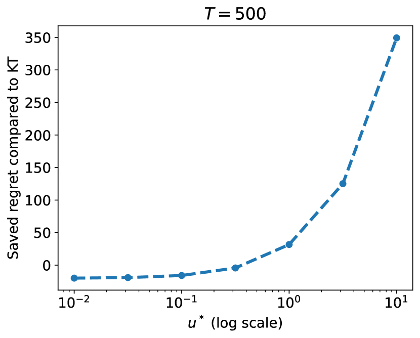
(b) Fix $T$ and vary $u^{*}$.

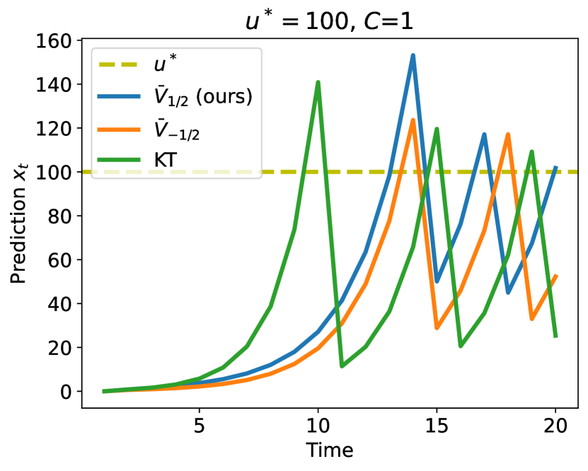
(c) The progression of $x_{t}$.

Figure 1: One-dimensional synthetic task with loss $|x_{t}-u^{*}|$. Specifically, Subfigure (b) fixes $T=500$ and plots $\mathrm{Regret}_{T}(u^{*})$ of KT minus $\mathrm{Regret}_{T}(u^{*})$ of our algorithm ($\bar{V}_{1/2}$) as a function of $u^{*}$.

6 Conclusion

We propose a framework that generates unconstrained OLO potentials by solving a PDE. It reduces the amount of guessing in the current workflow, thus simplifying the discovery and analysis of more complicated potentials. To demonstrate its power, we use this framework to design a concrete algorithm - it achieves the optimal loss-regret trade-off without any impractical doubling trick, and moreover, attains the optimal leading constant. Such properties lead to practical advantages when a good initialization is not available.

Overall, we feel the continuous-time perspective adopted in this paper, based on a series of recent works [19, 23], could be a powerful tool for adaptive online learning in general. Several interesting directions are left open:

• In order to further improve practicality, can we use the new potential to achieve gradient-adaptive [11, 13, 34] bounds?

• Can the PDE framework achieve adaptivity or trade-offs in a broader range of online learning problems? For example, with bandit feedback, switching cost, delays, etc.

• Is there a more principled way to handle the obtained PDEs, without enough boundary conditions? Can we automate the discovery and verification of new potentials?

Appendix

Organization

Appendix A presents details on the derivation of our PDE (5). Appendix B solves the one-dimensional PDE and verifies the quality of the induced coin-betting policies. Appendix C converts our theoretical results on coin-betting to unconstrained OLO. Appendix D presents details on our experiments.

Appendix A Detail on the derivation of PDE

In this section we present two aspects of our PDE derivation omitted in the main paper. First, we prove Lemma 2.2 which shows that any value function can naturally induce a pair of “dual” player-adversary policies. Next, we discuss our choice of scaling factors for the scaled game (Definition 2.2).

A.1 Proof of Lemma 2.2

See 2.2

Proof of Lemma 2.2.

We only prove the first part by induction. The proof of the second part is similar, therefore omitted. Let us restate the backward recursion (4),

$$V(t,S)=\min_{x\in\mathcal{X}}\max_{c\in\mathcal{C}}\left[{V(t+1,S+c)-\left\langle c,x\right\rangle}\right].$$

Starting from $t=0$ and $S=0$, let $x_{1}$ be the outer minimizing argument. Then, for all adversary policy $a_{1}$ such that $c_{1}=a_{1}(x_{1})$, we have $V(1,c_{1})=V(1,c_{1})-V(0,0)\leq\left\langle c_{1},x_{1}\right\rangle$.

Now consider the following induction hypothesis: there exists $T\in\mathbb{N}_{+}$, initial bet $x_{1}$ and functions $p^{*}_{2},\ldots,p^{*}_{T}$ such that for all $\bm{a}$,

$$\sum_{t=1}^{T}\left\langle c_{t},x_{t}\right\rangle\geq V\left({T,\sum_{t=1}^{T}c_{t}}\right).$$

Plugging $(t,S)=(T,\sum_{t=1}^{T}c_{t})$ into the backward recursion,

$$V\left({T,\sum_{t=1}^{T}c_{t}}\right)=\min_{x_{T+1}\in\mathcal{X}}\max_{c_{T+1}\in\mathcal{C}}\left[{V\left({T+1,\sum_{t=1}^{T+1}c_{t}}\right)-\left\langle c_{T+1},x_{T+1}\right\rangle}\right].$$

Given the value function $V$, there exists $x_{T+1}$ only depending on $T$ and $\sum_{t=1}^{T}c_{t}$ such that for all $c_{T+1}$,

$$V\left({T,\sum_{t=1}^{T}c_{t}}\right)\geq V\left({T+1,\sum_{t=1}^{T+1}c_{t}}\right)-\left\langle c_{T+1},x_{T+1}\right\rangle.$$

Define the policy $p^{*}_{T+1}$ in this way, we have

$$\sum_{t=1}^{T+1}\left\langle c_{t},x_{t}\right\rangle\geq V\left({T+1,\sum_{t=1}^{T+1}c_{t}}\right).\qed$$

A.2 The choice of scaling factors

We now discuss our choice of scaling factors for the scaled game (Definition 2.2). To begin with, let us review the wealth lower bounds for the existing coin-betting setting [32, 37] with budget constraints. For simplicity, assume $d=1$. Inspired by the celebrated Kelly bettor [25], McMahan and Abernethy [32] made an interesting observation: if starting from an initial wealth $C$ and knowing the bias of future coins ($\sum_{t=1}^{T}c_{t}/T$), the player could bet a fixed fraction $\beta=\sum_{t=1}^{T}c_{t}/T$ of his wealth in each round and guarantees a wealth lower bound

$$\mathrm{Wealth}_{T}\geq C\exp\left({\frac{(\sum_{t=1}^{T}c_{t})^{2}}{2T}}\right).$$ (14)

Of course, this strategy is not implementable in reality. However, using a time-dependent betting fraction $\beta_{t}$ that reflects the bias observed online, the player can actually implement a strategy [37] with

$$\mathrm{Wealth}_{T}\geq\frac{C}{\sqrt{T}}\exp\left({\frac{(\sum_{t=1}^{T}c_{t})^{2}}{2T}}\right),$$

which matches (14) in the important exponential factor. Under the presence of budget constraints, such an exponential factor is optimal. Extended to our unconstrained coin-betting setting (which is a strict generalization of the existing one), this exponential factor characterizes the best result when the player can only tolerate a fixed amount of total loss. This is intuitively similar to the concept of Pareto optimality: the optimal policy for the player depends on how risk-tolerant it is.

Back to the design of scaling factors for the $\varepsilon$-scaled game, our guideline is simple: the baseline strategy [32] discussed above should guarantee the same wealth bound in the scaled game and the original game. In this way, the PDE derived in the scaling limit could recover the specific Pareto optimal result (14). Concretely, let $f(\varepsilon)$ and $g(\varepsilon)$ be the scaling factors on the unit time and the coin space respectively. Without loss of generality, let $g(\varepsilon)=\varepsilon$; we now justify our choice $f(\varepsilon)=\varepsilon^{2}$.

Consider an extreme adversary whose decisions are always 1. In the original game, the baseline strategy [32] guarantees $\mathrm{Wealth}_{T}\geq C\exp(T/2)$ due to (14). In the scaled game, the adversary decisions are scaled by $\varepsilon$, and the total number of decision rounds is $[f(\varepsilon)]^{-1}$ times as many. Therefore, the baseline strategy [32] guarantees

$$\mathrm{Wealth}_{T}\geq C\exp\left({\frac{(\varepsilon T\cdot[f(\varepsilon)]^{-1})^{2}}{2T\cdot[f(\varepsilon)]^{-1}}}\right)=C\exp\left({\frac{\varepsilon^{2}T\cdot[f(\varepsilon)]^{-1}}{2}}\right).$$

If $f(\varepsilon)=\varepsilon^{2}$, then the wealth bounds for the scaled game and the original game are equal.

Appendix B Detail on the PDE-based betting policy

In this section we present detailed analysis of the one-dimensional coin-betting game (Section 3). By solving the backward heat equation (6), we obtain three specific limiting value functions (i.e., potential functions) $\bar{V}_{1}$, $\bar{V}_{-1/2}$ and $\bar{V}_{1/2}$. The performance of their induced coin-betting policies (Algorithm 3) will be characterized next.

In particular, $\bar{V}_{1}$ is a special case where the exact minimax relation (Lemma 2.2) can be directly applied. For the general case (e.g., $\bar{V}_{-1/2}$ and $\bar{V}_{1/2}$), the minimax relation only approximately holds, therefore we need to use a perturbed analysis introduced in Appendix B.2 to B.5. Finally, Appendix B.6 shows the optimality of the coin-betting policies.

B.1 Special case: Policy induced by $\bar{V}_{1}$

It is easy to verify that $\bar{V}_{1}(t,S)=C(S^{2}-t)$ satisfies Definition 2.1. Therefore, the performance guarantee of the associated player and adversary policies (Algorithm 2 and 3) can be stated as a corollary of Lemma 2.2.

Corollary 6.

For all $T\in\mathbb{N}_{+}$,

1. Against any adversary policy $\bm{a}$, Algorithm 3 constructed from $\bar{V}_{1}$ guarantees

   $$\mathrm{Wealth}_{T}\geq C\left[{\left({\sum_{t=1}^{T}c_{t}}\right)^{2}-T}\right].$$

2. Against any player policy $\bm{p}$, Algorithm 2 constructed from $\bar{V}_{1}$ guarantees

   $$\mathrm{Wealth}_{T}\leq C\left[{\left({\sum_{t=1}^{T}c_{t}}\right)^{2}-T}\right].$$

B.2 General case: Discrete Itô formula

In general, the solution of the backward heat equation (6) is only an approximation of a value function (for the discrete-time coin-betting game), therefore Lemma 2.1 cannot be directly applied. Instead, we pursue a perturbed analysis using the Discrete Itô formula. Harvey et al. used this technique in the two-expert LEA problem. Here we modify it for our coin-betting problem.

See 3.1

Proof of Lemma 3.1.

Starting from the LHS of (13),

$$LHS =\bar{V}\left({t+1,\sum_{i=1}^{t+1}c_{i}}\right)-\frac{1}{2}\left[{\bar{V}\left({t+1,\sum_{i=1}^{t}c_{i}+1}\right)+\bar{V}\left({t+1,\sum_{i=1}^{t}c_{i}-1}\right)}\right]$$

$$\hskip 85.35826pt+\frac{1}{2}\left[{\bar{V}\left({t+1,\sum_{i=1}^{t}c_{i}+1}\right)+\bar{V}\left({t+1,\sum_{i=1}^{t}c_{i}-1}\right)}\right]-\bar{V}\left({t,\sum_{i=1}^{t}c_{i}}\right)$$

$$=\bar{V}\left({t+1,\sum_{i=1}^{t+1}c_{i}}\right)-\frac{1}{2}\left[{\bar{V}\left({t+1,\sum_{i=1}^{t}c_{i}+1}\right)+\bar{V}\left({t+1,\sum_{i=1}^{t}c_{i}-1}\right)}\right]$$

$$\hskip 85.35826pt+\bar{\nabla}_{t}\bar{V}\left({t+1,\sum_{i=1}^{t}c_{i}}\right)+\frac{1}{2}\bar{\nabla}_{SS}\bar{V}\left({t+1,\sum_{i=1}^{t}c_{i}}\right).$$

The remaining task is to show

$$\bar{V}\left({t+1,\sum_{i=1}^{t+1}c_{i}}\right)-\frac{1}{2}\left[{\bar{V}\left({t+1,\sum_{i=1}^{t}c_{i}+1}\right)+\bar{V}\left({t+1,\sum_{i=1}^{t}c_{i}-1}\right)}\right]\leq c_{t+1}x_{t+1}.$$

Plugging in the player’s bet $x_{t+1}$ (11), it suffices to show that

$$\bar{V}\left({t+1,\sum_{i=1}^{t+1}c_{i}}\right)\leq\frac{1+c_{t+1}}{2}\bar{V}\left({t+1,\sum_{i=1}^{t}c_{i}+1}\right)+\frac{1-c_{t+1}}{2}\bar{V}\left({t+1,\sum_{i=1}^{t}c_{i}-1}\right),$$

which follows from the convexity of $\bar{V}$. Equality is achieved when $c_{t+1}\in\{-1,1\}$. ∎

B.3 Preliminary: Properties of $\bar{V}_{1/2}$ and $\bar{V}_{-1/2}$

In the Discrete Itô formula, quantifying the perturbation term $\Diamond$ is case-dependent. Before doing so, we present some facts on $\bar{V}_{1/2}$ and $\bar{V}_{-1/2}$ which will be useful later. Let us first consider $\bar{V}_{1/2}$. For clarity, we copy the definition here.

$$\bar{V}_{1/2}(t,S)=C\sqrt{t}\left[{2\int_{0}^{S/\sqrt{2t}}\left({\int_{0}^{u}\exp(x^{2})dx}\right)du-1}\right].$$

Some calculation yields its derivatives. Let $\nabla_{t}$ and $\nabla_{tt}$ be the first and second order derivative with respect to $t$. Let $\nabla_{S}$, $\nabla_{SS}$, $\nabla_{SSS}$, $\nabla_{SSSS}$ be the first to fourth order derivative with respect to $S$.

$$\nabla_{S}\bar{V}_{1/2}(t,S)=\sqrt{2}C\int_{0}^{S/\sqrt{2t}}\exp(x^{2})dx.$$

$$\nabla_{SS}\bar{V}_{1/2}(t,S)=\frac{C}{\sqrt{t}}\exp\left({\frac{S^{2}}{2t}}\right).$$

$$\nabla_{SSS}\bar{V}_{1/2}(t,S)=\frac{CS}{t^{3/2}}\exp\left({\frac{S^{2}}{2t}}\right).$$

$$\nabla_{SSSS}\bar{V}_{1/2}(t,S)=\frac{C}{t^{3/2}}\exp\left({\frac{S^{2}}{2t}}\right)\left({\frac{S^{2}}{t}+1}\right).$$

$$\nabla_{t}\bar{V}_{1/2}(t,S)=-\frac{C}{2\sqrt{t}}\exp\left({\frac{S^{2}}{2t}}\right).$$

$$\nabla_{tt}\bar{V}_{1/2}(t,S)=\frac{C}{4t^{3/2}}\exp\left({\frac{S^{2}}{2t}}\right)\left({\frac{S^{2}}{t}+1}\right).$$

Similarly, for $\bar{V}_{-1/2}$ we have the following.

$$\bar{V}_{-1/2}(t,S)=\frac{C}{\sqrt{t}}\exp\left({\frac{S^{2}}{2t}}\right).$$

$$\nabla_{S}\bar{V}_{-1/2}(t,S)=\frac{CS}{t^{3/2}}\exp\left({\frac{S^{2}}{2t}}\right).$$

$$\nabla_{SS}\bar{V}_{-1/2}(t,S)=\frac{C}{t^{3/2}}\exp\left({\frac{S^{2}}{2t}}\right)\left({\frac{S^{2}}{t}+1}\right).$$

$$\nabla_{SSS}\bar{V}_{-1/2}(t,S)=\frac{C}{t^{3/2}}\exp\left({\frac{S^{2}}{2t}}\right)\left({\frac{S^{3}}{t^{2}}+\frac{3S}{t}}\right).$$

$$\nabla_{SSSS}\bar{V}_{-1/2}(t,S)=\frac{C}{t^{5/2}}\exp\left({\frac{S^{2}}{2t}}\right)\left({\frac{S^{4}}{t^{2}}+\frac{6S^{2}}{t}+3}\right).$$

$$\nabla_{t}\bar{V}_{-1/2}(t,S)=-\frac{C}{2t^{3/2}}\exp\left({\frac{S^{2}}{2t}}\right)\left({\frac{S^{2}}{t}+1}\right).$$

$$\nabla_{tt}\bar{V}_{-1/2}(t,S)=\frac{C}{4t^{5/2}}\exp\left({\frac{S^{2}}{2t}}\right)\left({\frac{S^{4}}{t^{2}}+\frac{6S^{2}}{t}+3}\right).$$

Let us compare the betting behavior induced by $\bar{V}_{1/2}$ and $\bar{V}_{-1/2}$. The bets in both cases are roughly their derivatives.

Lemma B.1.

For all $t\in\mathbb{N}_{+}$ and $\left|{S}\right|\leq t-1$, $|\nabla_{S}\bar{V}_{1/2}(t,S)|\geq|\nabla_{S}\bar{V}_{-1/2}(t,S)|$.

Proof of Lemma B.1.

Due to symmetry, it suffices to consider $0\leq S\leq t-1$. Notice that when $S=0$, $\nabla_{S}\bar{V}_{1/2}(t,0)=\nabla_{S}\bar{V}_{-1/2}(t,0)$. With $S\leq t-1$,

$$\frac{\nabla_{SS}\bar{V}_{-1/2}(t,S)}{\nabla_{SS}\bar{V}_{1/2}(t,S)}=\frac{1}{t}\left({\frac{S^{2}}{t}+1}\right)\leq 1-t^{-1}+t^{-2}\leq 1.\qed$$

Moreover, let us specifically compare the derivatives when $|S|=O(\sqrt{t})$: $|\nabla_{S}\bar{V}_{1/2}(t,S)|=O(1)$ while $|\nabla_{S}\bar{V}_{-1/2}(t,S)|=O(t^{-1})$. Therefore, the betting behavior induced by $\bar{V}_{1/2}$ cannot be achieved by simply scaling $\bar{V}_{-1/2}$ (i.e., using a different $C$).

Finally back to $\bar{V}_{1/2}$, the integral definition may not be easy to interpret. We can further lower bound it as the following.

Lemma B.2.

For all $(t,S)$ such that $\sqrt{2t}\leq|S|\leq t$,

$$\bar{V}_{1/2}(t,S)\geq C\sqrt{t}\cdot\left[{\frac{t}{S^{2}}\exp\left({\frac{S^{2}}{2t}}\right)-\frac{3}{2}}\right].$$

Proof of Lemma B.2.

Based on the definition of $\bar{V}_{1/2}$, it suffices to show that for all $z\geq 1$,

$$f(z)\mathrel{\mathop{:}}=2\int_{0}^{z}\left({\int_{0}^{u}\exp(x^{2})dx}\right)du-\frac{1}{2z^{2}}\exp\left({z^{2}}\right)\geq-1/2.$$

Notice that $f(1)\geq-1/2$. Taking the derivatives,

$$f^{\prime}(z)=2\int^{z}_{0}\exp(x^{2})dx+\exp(z^{2})\left[{z^{-3}-z^{-1}}\right].$$

$f^{\prime}(1)\geq 0$, and

$$f^{\prime\prime}(z)=3\exp\left({z^{2}}\right)\left({z^{-2}-z^{-4}}\right)\geq 0.\qed$$

B.4 Policy induced by $\bar{V}_{1/2}$

In this subsection we characterize the player policy constructed from $\bar{V}_{1/2}$. The first step is to quantify the perturbation error ($\Diamond$ in (13)). After that, the wealth lower bound (Theorem 1) follows from a telescopic sum on the Discrete Itô formula.

See 3.2

Proof of Lemma 3.2.

Plugging in the definition of discrete derivative,

$$\bar{\nabla}_{t}\bar{V}_{1/2}(t,S)+\bar{\nabla}_{SS}\bar{V}_{1/2}(t,S)/2=\frac{1}{2}\bar{V}_{1/2}(t,S+1)+\frac{1}{2}\bar{V}_{1/2}(t,S-1)-\bar{V}_{1/2}(t-1,S).$$ (15)

Step 1: upper bound.

For clarity, define a function $f:\mathbb{R}\rightarrow\mathbb{R}$ as

$$f(z)=2z\int_{0}^{z}\exp(x^{2})dx-\exp(z^{2}).$$

Then, using the definition of $\bar{V}_{1/2}$, it suffices to show that

$$f\left({-\frac{1}{\sqrt{2}}}\right)+f\left({\frac{1}{\sqrt{2}}}\right)\leq 0,$$

and for all $t>1$,

$$f\left({\frac{S-1}{\sqrt{2t}}}\right)+f\left({\frac{S+1}{\sqrt{2t}}}\right)\leq 2\sqrt{1-\frac{1}{t}}f\left({\frac{S}{\sqrt{2(t-1)}}}\right).$$

The first inequality can be easily verified by computing the values of $f(1/\sqrt{2})$ and $f(-1/\sqrt{2})$. As for the second inequality, we use an existing result [23, Lemma C.4]: for all $x\in\mathbb{R}$ and $z\in[0,1)$,

$$f\left({\frac{x-z}{\sqrt{2}}}\right)+f\left({\frac{x+z}{\sqrt{2}}}\right)\leq 2\sqrt{1-z^{2}}f\left({\frac{x}{\sqrt{2(1-z^{2})}}}\right).$$

Taking $x=S/\sqrt{t}$ and $z=1/\sqrt{t}$ completes the proof.

Step 2: lower bound.

From Taylor’s theorem,

$$\bar{V}_{1/2}(t,S+1)=\bar{V}_{1/2}(t,S)+\nabla_{S}\bar{V}_{1/2}(t,S)+\frac{1}{2}\nabla_{SS}\bar{V}_{1/2}(t,S)+\frac{1}{6}\nabla_{SSS}\bar{V}_{1/2}(t,S)+\frac{1}{24}\nabla_{SSSS}\bar{V}_{1/2}(t,S+a),$$

$$\bar{V}_{1/2}(t,S-1)=\bar{V}_{1/2}(t,S)-\nabla_{S}\bar{V}_{1/2}(t,S)+\frac{1}{2}\nabla_{SS}\bar{V}_{1/2}(t,S)-\frac{1}{6}\nabla_{SSS}\bar{V}_{1/2}(t,S)+\frac{1}{24}\nabla_{SSSS}\bar{V}_{1/2}(t,S-b),$$

$$\bar{V}_{1/2}(t-1,S)=\bar{V}_{1/2}(t,S)-\nabla_{t}\bar{V}_{1/2}(t,S)+\frac{1}{2}\nabla_{tt}\bar{V}_{1/2}(t-c,S),$$

where $a,b,c\in[0,1]$. Plugging these into (15) and using the condition $\nabla_{t}\bar{V}_{1/2}=-\nabla_{SS}\bar{V}_{1/2}/2$ (since $\bar{V}_{1/2}$ is a solution of the backward heat equation), we have

$$\bar{\nabla}_{t}\bar{V}_{1/2}(t,S)+\bar{\nabla}_{SS}\bar{V}_{1/2}(t,S)/2=\frac{1}{48}\nabla_{SSSS}\bar{V}_{1/2}(t,S+a)+\frac{1}{48}\nabla_{SSSS}\bar{V}_{1/2}(t,S-b)-\frac{1}{2}\nabla_{tt}\bar{V}_{1/2}(t-c,S).$$

From Appendix B.3, $\nabla_{SSSS}\bar{V}_{1/2}(t,S)\geq 0$ for all $(t,S)$, and

$$\nabla_{tt}\bar{V}_{1/2}(t,S)=\frac{C}{4}t^{-3/2}\exp\left({\frac{S^{2}}{2t}}\right)\left({\frac{S^{2}}{t}+1}\right).$$

Therefore,

$$\bar{\nabla}_{t}\bar{V}_{1/2}(t,S)+\bar{\nabla}_{SS}\bar{V}_{1/2}(t,S)/2 \geq-\frac{C}{8}\max_{c\in[0,1]}(t-c)^{-3/2}\exp\left({\frac{S^{2}}{2(t-c)}}\right)\left({\frac{S^{2}}{t-c}+1}\right)$$

$$=-\frac{C}{8}(t-1)^{-3/2}\exp\left({\frac{S^{2}}{2(t-1)}}\right)\left({\frac{S^{2}}{t-1}+1}\right).\qed$$

Next we prove Theorem 2. It shows that the wealth lower bound (Theorem 1) faithfully characterizes the performance of the player policy constructed from $\bar{V}_{1/2}$.

See 2

Proof of Theorem 2.

We first construct the coin sequence. For all $S\in[-T,T]$, there exists an integer $\tilde{S}$ such that $|\tilde{S}|\leq T$, $(|\tilde{S}|+1)\bmod 2=T\bmod 2$ and $|S-\tilde{S}|\leq 1$. We define the coins using three phases.

1. $c_{1}=S-\tilde{S}$;

2. For all $1<t\leq T-|\tilde{S}|$, let $c_{t}=\text{sign}(c_{1})\cdot(-1)^{t-1}$;

3. If $\tilde{S}\neq 0$, then for all $t$ such that $T-|\tilde{S}|<t\leq T$, let $c_{t}=\tilde{S}/|\tilde{S}|$.

Based on this coin sequence, there are three immediate observations:

1. The sum of coins from the second phase is 0, and the sum of coins from the third phase is $\tilde{S}$; therefore, $\sum_{t=1}^{T}c_{t}=S$.

2. If $\tau\leq T-|\tilde{S}|$ then $|\sum_{t=1}^{\tau}c_{t}|\leq 1$.

3. If $T-|\tilde{S}|<\tau\leq T$ then $|\sum_{t=1}^{\tau}c_{t}|=|S|-T+\tau$.

Next, we derive the wealth upper bound induced by such a coin sequence and the player policy (Algorithm 3). Starting from the first round, $x_{1}=0$, therefore $\mathrm{Wealth}_{1}=0$. $\mathrm{Wealth}_{1}=\bar{V}_{1/2}(1,c_{1})-\bar{V}_{1/2}(1,c_{1})\leq\bar{V}_{1/2}(1,c_{1})-\bar{V}_{1/2}(1,0)=\bar{V}_{1/2}(1,c_{1})+C$. Considering the rest of the rounds, there are two cases: ($i$) $|S|\leq\sqrt{T}$; ($ii$) $|S|>\sqrt{T}$.

Case ($i$)

In this case we first show that for all integer $\tau$ in $[1:T]$, $|\sum_{t=1}^{\tau}c_{t}|\leq\sqrt{\tau}$. Due to the second observation above, this condition holds for all $\tau\leq T-|\tilde{S}|$, and we only need to focus on $T-|\tilde{S}|<\tau\leq T$ (the third phase) where $|\sum_{t=1}^{\tau}c_{t}|=|S|-T+\tau\leq\sqrt{T}-T+\tau$; since $T-\sqrt{T}\geq\tau-\sqrt{\tau}$, we further have $|\sum_{t=1}^{\tau}c_{t}|\leq\sqrt{\tau}$. Based on this result, telescoping Lemma 3.1 (notice that equality is achieved) and using Lemma 3.2, we have

$$\mathrm{Wealth}_{T} \leq\bar{V}_{1/2}\left({T,\sum_{t=1}^{T}c_{t}}\right)+C+\frac{C}{8}\sum_{t=1}^{T-1}t^{-3/2}\exp\left({\frac{(\sum_{i=1}^{t}c_{i})^{2}}{2t}}\right)\left({\frac{(\sum_{i=1}^{t}c_{i})^{2}}{t}+1}\right)$$

$$\leq\bar{V}_{1/2}\left({T,\sum_{t=1}^{T}c_{t}}\right)+C+\frac{\sqrt{e}C}{4}\sum_{t=1}^{T-1}t^{-3/2}\leq\bar{V}\left({T,\sum_{t=1}^{T}c_{t}}\right)+\left({\frac{3\sqrt{e}}{4}+1}\right)C.$$

Case ($ii$)

In this case we show that for all integer $\tau$ in $[1:T]$, $|\sum_{t=1}^{\tau}c_{t}|/\sqrt{\tau}\leq|\sum_{t=1}^{T}c_{t}|/\sqrt{T}$. Similar to Case ($i$), we consider $\tau\leq T-|\tilde{S}|$ and $T-|\tilde{S}|<\tau\leq T$ separately. When $\tau\leq T-|\tilde{S}|$, we have $|\sum_{t=1}^{\tau}c_{t}|/\sqrt{\tau}\leq 1\leq|S|/\sqrt{T}=|\sum_{t=1}^{T}c_{t}|/\sqrt{T}$. On the other hand, when $T-|\tilde{S}|<\tau\leq T$ it suffices to show that

$$\frac{|S|-T+\tau}{\sqrt{\tau}}\leq\frac{|S|}{\sqrt{T}}.$$

The LHS monotonically increases with respect to $\tau$, and when $\tau=T$ the inequality holds with equality. In summary, the required condition $|\sum_{t=1}^{\tau}c_{t}|/\sqrt{\tau}\leq|\sum_{t=1}^{T}c_{t}|/\sqrt{T}$ holds for all $\tau\in[1:T]$.

Based on this result, telescoping Lemma 3.1 and using Lemma 3.2, we have

$$\mathrm{Wealth}_{T} \leq\bar{V}_{1/2}\left({T,\sum_{t=1}^{T}c_{t}}\right)+C+\frac{C}{8}\exp\left({\frac{(\sum_{i=1}^{T}c_{i})^{2}}{2T}}\right)\left({\frac{(\sum_{i=1}^{T}c_{i})^{2}}{T}+1}\right)\sum_{t=1}^{T-1}t^{-3/2}$$

$$\leq\bar{V}_{1/2}\left({T,\sum_{t=1}^{T}c_{t}}\right)+C+\frac{3C}{8}\exp\left({\frac{(\sum_{i=1}^{T}c_{i})^{2}}{2T}}\right)\left({\frac{(\sum_{i=1}^{T}c_{i})^{2}}{T}+1}\right).$$

Combining Case ($i$) and Case ($ii$) completes the proof. ∎

Theorem 2 has a special form: it fixes both the player policy (Algorithm 3) and the adversary policy (Algorithm 2), and then bounds the wealth induced by both of them. Results of this form are seldom studied in conventional online learning settings. The reason is that, the performance metric for those settings is usually the uniform regret (a real number), therefore the gap between policy-independent upper and lower bounds is relatively easy to describe. In contrast, we care about the trade-offs on our performance metric, so our upper and lower bounds are both expressed as functions; the characterization of their gap is much richer. We present our player-policy-independent wealth upper bound as Theorem 3. It is related, but incomparable to Theorem 2 stated above.

B.5 Policy induced by $\bar{V}_{-1/2}$

Analogous to the previous subsection, we now characterize the performance of the player policy induced by $\bar{V}_{-1/2}$. The first step is to quantify the perturbation error $\Diamond$.

Lemma B.3.

For all $t\in\mathbb{N}_{+}$ and $S\in[1-t,t-1]$, $\bar{V}_{-1/2}$ with any parameter $C>0$ satisfies the following conditions.

1. If $t=1$, then

   $$\bar{\nabla}_{t}\bar{V}_{-1/2}(t,S)+\bar{\nabla}_{SS}\bar{V}_{-1/2}(t,S)/2=C\sqrt{e}.$$

2. If $t>1$, then

   $$-\frac{C}{8}(t-1)^{-5/2}\exp\left({\frac{S^{2}}{2(t-1)}}\right)\left({\frac{S^{4}}{(t-1)^{2}}+\frac{6S^{2}}{t-1}+3}\right)\leq\bar{\nabla}_{t}\bar{V}_{-1/2}(t,S)+\bar{\nabla}_{SS}\bar{V}_{-1/2}(t,S)/2\leq 0.$$

Proof of Lemma B.3.

The case of $t=1$ can be easily verified. We will prove the second case next. Plugging in the definition, we have

$$\bar{\nabla}_{t}\bar{V}_{-1/2}(t,S)+\bar{\nabla}_{SS}\bar{V}_{-1/2}(t,S)/2 =\frac{1}{2}\bar{V}_{-1/2}(t,S+1)+\frac{1}{2}\bar{V}_{-1/2}(t,S-1)-\bar{V}_{-1/2}(t-1,S)$$

$$=\frac{C}{2\sqrt{t}}\exp\left({\frac{(S-1)^{2}}{2t}}\right)+\frac{C}{2\sqrt{t}}\exp\left({\frac{(S+1)^{2}}{2t}}\right)-\frac{C}{\sqrt{t-1}}\exp\left({\frac{S^{2}}{2(t-1)}}\right).$$ (16)

First, let us consider the upper bound. Since $\exp(-t^{-1})\geq 1-t^{-1}$, we have

$$\exp\left({\frac{1}{2t}}\right)\leq\sqrt{\frac{t}{t-1}}.$$

Therefore,

$$\exp\left({\frac{(S-1)^{2}}{2t}}\right)+\exp\left({\frac{(S+1)^{2}}{2t}}\right) =\exp\left({\frac{S^{2}+1}{2t}}\right)\left[{\exp\left({-\frac{S}{t}}\right)+\exp\left({\frac{S}{t}}\right)}\right]$$

$$\leq\sqrt{\frac{t}{t-1}}\exp\left({\frac{S^{2}}{2t}}\right)\left[{\exp\left({-\frac{S}{t}}\right)+\exp\left({\frac{S}{t}}\right)}\right]$$

$$\leq 2\sqrt{\frac{t}{t-1}}\exp\left({\frac{S^{2}}{2t}}\right)\exp\left({\frac{S^{2}}{2t^{2}}}\right),$$

where the last inequality is due to the classical result $\cosh(x)\leq\exp(x^{2}/2)$. Back to (16),

$$\bar{\nabla}_{t}\bar{V}_{-1/2}(t,S)+\bar{\nabla}_{SS}\bar{V}_{-1/2}(t,S)/2\leq C\sqrt{\frac{1}{t-1}}\left[{\exp\left({\frac{S^{2}}{2t}}\right)\exp\left({\frac{S^{2}}{2t^{2}}}\right)-\exp\left({\frac{S^{2}}{2(t-1)}}\right)}\right],$$

and it is straightforward to verify that $\text{RHS}\leq 0$.

Next, we consider the lower bound. Similar to the proof of Lemma 3.2, using the derivatives from Appendix B.3,

$$\bar{\nabla}_{t}\bar{V}_{-1/2}(t,S)+\bar{\nabla}_{SS}\bar{V}_{-1/2}(t,S)/2 \geq-\frac{1}{2}\nabla_{tt}\bar{V}_{-1/2}(t-1,S)$$

$$=-\frac{C}{8}(t-1)^{-5/2}\exp\left({\frac{S^{2}}{2(t-1)}}\right)\left({\frac{S^{4}}{(t-1)^{2}}+\frac{6S^{2}}{t-1}+3}\right).\qed$$

Similar to the wealth lower bound induced by $\bar{V}_{1/2}$ (Theorem 1), we can plug the above lemma into the Discrete Itô formula (Lemma 3.1) and obtain the following theorem via a telescopic sum. The proof is omitted. Essentially, a wealth lower bound of this form recovers the result from [37]. However, our analysis is based on a general framework without budget constraints, therefore does not involve any betting fractions.

Theorem 7.

For all $T\in\mathbb{N}_{+}$, Algorithm 3 constructed from $\bar{V}_{-1/2}$ guarantees a wealth lower bound

$$\mathrm{Wealth}_{T}\geq\bar{V}_{-1/2}\left({T,\sum_{t=1}^{T}c_{t}}\right)-C\sqrt{e},$$

against any adversary policy $\bm{a}$.

In addition, analogous to Theorem 2, we can also state a wealth upper bound based on $\bar{V}_{-1/2}$. The proof uses a similar strategy, therefore is omitted.

Theorem 8.

For all $T\in\mathbb{N}_{+}$ and $S\in[-T,T]$, we can construct $c_{1}\in\mathcal{C}$ and $c_{2},\ldots,c_{T}\in\{-1,1\}$ such that

1. $\sum_{t=1}^{T}c_{t}=S$;

2. If the player applies Algorithm 3 constructed from $\bar{V}_{-1/2}$ (with parameter $C$) and the adversary plays the aforementioned coin sequence $c_{1:T}$, then

   $$\mathrm{Wealth}_{T}\leq\bar{V}_{-1/2}\left({T,S}\right)+\frac{5C}{24}\exp\left({\frac{S^{2}}{2T}}\right)\left({\frac{S^{4}}{T^{2}}+\frac{6S^{2}}{T}+3}\right)+2C.$$

B.6 The optimality of betting policies

Finally, we prove the player-policy-independent wealth upper bounds (Theorem 3 and its analogue based on $\bar{V}_{-1/2}$). The first step is to prove a sharp lower bound for the tail probability of one-dimensional symmetric random walk, based on a normal approximation.

Lemma B.4.

For all $T\in\mathbb{N}_{+}$, let $z_{1},\ldots,z_{T}$ be i.i.d. Rademacher random variables. Then for any $k>0$,

$$\mathbb{P}\left[{\left|{\sum_{t=1}^{T}z_{t}}\right|\geq k}\right]\geq\sqrt{\frac{2}{\pi}}\frac{k\sqrt{T}}{k^{2}+T}\exp\left({-\frac{k^{2}}{2T}}\right)-\frac{1}{\sqrt{T}}.$$

Proof of Lemma B.4.

Due to Central Limit Theorem, the random variable $(\sum_{t=1}^{T}z_{t})/\sqrt{T}$ converges in distribution to standard normal $N(0,1)$. Concretely, the nonasymptotic convergence rate can be characterized via the Berry-Esseen Theorem [30]: Let $F_{T}(x)$ be the CDF of $(\sum_{t=1}^{T}z_{t})/\sqrt{T}$ and $\Phi(x)$ be the standard normal CDF, then,

$$\sup_{x\in\mathbb{R}}\left|{F_{T}(x)-\Phi(x)}\right|\leq\frac{1}{2\sqrt{T}}.$$

For the tail probability of standard normal distribution, there is a standard lower bound [22] through the Mills ratio, which can be verified via a derivative argument: For all $x>0$,

$$1-\Phi(x)\geq\frac{1}{\sqrt{2\pi}}\frac{1}{x+x^{-1}}\exp\left({-\frac{x^{2}}{2}}\right).$$

Therefore,

$$\mathbb{P}\left[{\left|{\sum_{t=1}^{T}z_{t}}\right|\geq k}\right]=2\cdot\left[{1-F_{T}(k/\sqrt{T})}\right]\geq 2\cdot\left[{1-\Phi(k/\sqrt{T})-\frac{1}{2\sqrt{T}}}\right]\geq\sqrt{\frac{2}{\pi}}\frac{k\sqrt{T}}{k^{2}+T}\exp\left({-\frac{k^{2}}{2T}}\right)-\frac{1}{\sqrt{T}}.\qed$$

Compared to similar tail lower bounds from existing works on unconstrained OLO [36, 38], Lemma B.4 has the tight exponent (1/2) in the exponential function. This allows us to justify the optimality of our PDE-based coin-betting policy (Algorithm 3 constructed from $\bar{V}_{1/2}$), and eventually the converted unconstrained OLO algorithm.

See 3

Proof of Theorem 3.

Let us first generalize the unconstrained coin-betting game to allow random adversary on the coin space $\{-1,1\}$. That is, based on past player bets $x_{1},\ldots,x_{t}$, the adversary decides a distribution on $\{-1,1\}$ and samples $c_{t}$ from this distribution.

Now, consider the setting where the player applies any policy $\bm{p}$ that guarantees $\mathrm{Wealth}_{T}\geq-C\sqrt{T}$, and the adversary picks coin outcomes according to a Rademacher distribution: regardless of $x_{1},\ldots,x_{t}$, the coin $c_{t}$ equals $-1$ and $1$ with probability $1/2$ respectively. Then for all $T\in\mathbb{N}_{+}$, let $k=\sqrt{2T\log\lambda}$.

$$0 =\mathbb{E}\left[{\sum_{t=1}^{T}c_{t}x_{t}}\right]$$

$$=\mathbb{E}\left[{\sum_{t=1}^{T}c_{t}x_{t}\bigg{|}\left|{\sum_{t=1}^{T}c_{t}}\right|\geq k}\right]\mathbb{P}\left[{\left|{\sum_{t=1}^{T}c_{t}}\right|\geq k}\right]+\mathbb{E}\left[{\sum_{t=1}^{T}c_{t}x_{t}\bigg{|}\left|{\sum_{t=1}^{T}c_{t}}\right|<k}\right]\mathbb{P}\left[{\left|{\sum_{t=1}^{T}c_{t}}\right|<k}\right]$$

$$\geq\mathbb{E}\left[{\sum_{t=1}^{T}c_{t}x_{t}\bigg{|}\left|{\sum_{t=1}^{T}c_{t}}\right|\geq k}\right]\mathbb{P}\left[{\left|{\sum_{t=1}^{T}c_{t}}\right|\geq k}\right]-C\sqrt{T}.$$

Applying Lemma B.4, using $\lambda\geq\exp[(\sqrt{2}+1)/2]$ and $T\geq 8\pi\lambda^{2}\log\lambda$,

$$\mathbb{P}\left[{\left|{\sum_{t=1}^{T}c_{t}}\right|\geq k}\right] \geq\sqrt{\frac{2}{\pi}}\frac{\sqrt{2\log\lambda}}{1+2\log\lambda}\lambda^{-1}-\frac{1}{\sqrt{T}}$$

$$\geq\frac{1}{\sqrt{2\pi\log\lambda}}\lambda^{-1}-\frac{1}{\sqrt{T}}\geq\frac{1}{2\sqrt{2\pi\log\lambda}}\lambda^{-1}.$$

$$\mathbb{E}\left[{\sum_{t=1}^{T}c_{t}x_{t}\bigg{|}\left|{\sum_{t=1}^{T}c_{t}}\right|\geq k}\right]\leq\frac{C\sqrt{T}}{\mathbb{P}\left[{\left|{\sum_{t=1}^{T}c_{t}}\right|\geq k}\right]}\leq 2\sqrt{2\pi}\lambda\sqrt{\log\lambda}\cdot C\sqrt{T}.$$

Therefore, for any player policy $\bm{p}$ there exists an adversary policy $\bm{a}$ which induces $|\sum_{t=1}^{T}c_{t}|\geq\sqrt{2T\log\lambda}$ and $\mathrm{Wealth}_{T}\leq 2\sqrt{2\pi}\lambda\sqrt{\log\lambda}\cdot C\sqrt{T}$. ∎

A similar result can be stated with respect to $\bar{V}_{-1/2}$, using a different “barrier” $k$ that depends on $T$. This introduces a specific technical issue: when we use Lemma B.4, the normal approximation error ($1/\sqrt{T}$) is comparable in magnitude to the Gaussian tail bound (the first term in Lemma B.4) which we care about. Therefore, the following theorem has a slightly weaker form than Theorem 3.

Theorem 9.

For all $\lambda\geq\exp[(\sqrt{2}+1)/2]$, there exists $T_{0}\in\mathbb{N}_{+}$ (depending on $\lambda$) such that for all $T\geq T_{0}$ and any player policy $\bm{p}$ which guarantees $\mathrm{Wealth}_{T}\geq-C\sqrt{e}$ (e.g., Algorithm 3 constructed from $\bar{V}_{-1/2}$), there exists an adversary policy $\bm{a}$ with the following property. In the coin-betting game induced by the policy pair $(\bm{p},\bm{a})$,

1. $|\sum_{t=1}^{T}c_{t}|\geq\sqrt{2T\log(\lambda\sqrt{T}/\log T)}$;

2. $\mathrm{Wealth}_{T}\leq 2\sqrt{2\pi e}\lambda(\log T)^{-1}\sqrt{\log(\lambda\sqrt{T}/\log T)}\cdot C\sqrt{T}$.

Proof of Theorem 9.

We follow a similar analysis as Theorem 3 but use a different barrier. Let us only consider $T>1$ and let $k=\sqrt{2T\log(\lambda\sqrt{T}/\log T)}$. Using the Rademacher random adversary,

$$\mathbb{E}\left[{\sum_{t=1}^{T}c_{t}x_{t}\bigg{|}\left|{\sum_{t=1}^{T}c_{t}}\right|\geq k}\right]\mathbb{P}\left[{\left|{\sum_{t=1}^{T}c_{t}}\right|\geq k}\right]\leq C.$$

Using $\lambda\geq\exp[(\sqrt{2}+1)/2]$, we have $1\leq 2(\sqrt{2}-1)\log(\lambda)\leq 2(\sqrt{2}-1)\log(\lambda\sqrt{T}/\log T)$. Therefore,

$$\mathbb{P}\left[{\left|{\sum_{t=1}^{T}c_{t}}\right|\geq k}\right] \geq\sqrt{\frac{2}{\pi}}\frac{\sqrt{2\log(\lambda\sqrt{T}/\log T)}}{1+2\log(\lambda\sqrt{T}/\log T)}\frac{\log T}{\lambda\sqrt{T}}-\frac{1}{\sqrt{T}}$$

$$\geq\frac{\log T}{\lambda\sqrt{2\pi\log(\lambda\sqrt{T}/\log T)}}T^{-1/2}-T^{-1/2}.$$

Since the first term decays slower (with respect to $T$) than the second term $T^{-1/2}$, there exists $T_{0}$ depending on $\lambda$ such that for all $T\geq T_{0}$,

$$\mathbb{P}\left[{\left|{\sum_{t=1}^{T}c_{t}}\right|\geq k}\right]\geq\frac{\log T}{2\lambda\sqrt{2\pi\log(\lambda\sqrt{T}/\log T)}}T^{-1/2},$$

$$\mathbb{E}\left[{\sum_{t=1}^{T}c_{t}x_{t}\bigg{|}\left|{\sum_{t=1}^{T}c_{t}}\right|\geq k}\right]\leq\frac{C\sqrt{e}}{\mathbb{P}\left[{\left|{\sum_{t=1}^{T}c_{t}}\right|\geq k}\right]}\leq 2\sqrt{2\pi e}\lambda(\log T)^{-1}\sqrt{\log(\lambda\sqrt{T}/\log T)}\cdot C\sqrt{T}.\qed$$

Appendix C Detail on unconstrained OLO

In this section we present detailed analysis on unconstrained OLO. First, using the conversion from coin-betting to OLO (Algorithm 1), our coin-betting policy (Algorithm 3) can be directly converted into a one-dimensional unconstrained OLO algorithm. For clarity, we restate its pseudo-code as Algorithm 5.

Algorithm 5 PDE-based one-dimensional unconstrained OLO algorithm.

0:  A one-dimensional limiting value function $\bar{V}$ which satisfies (6).

1:  for $t=1,2,\ldots$ do

2:     Predict

$$x_{t}=\frac{1}{2}\left[{\bar{V}\left({t,-\sum_{i=1}^{t-1}g_{i}+1}\right)-\bar{V}\left({t,-\sum_{i=1}^{t-1}g_{i}-1}\right)}\right].$$

3:     Observe the loss gradient $g_{t}$ and store it.

4:  end for

For general $d$-dimensional problems, we rely on a classical reduction [11] to the one-dimensional problem. Its pseudo-code is Algorithm 6, and the associated performance guarantee is Lemma C.1 whose proof follows from [11, Theorem 2] and the standard regret bound of OGD (e.g., [39, Section 4.2.1]). Our final product is Algorithm 4 presented in the main paper.

Algorithm 6 Reducing unconstrained OLO from $\mathbb{R}^{d}$ to $\mathbb{R}$.

0:  A one-dimensional unconstrained OLO algorithm $\mathcal{A}_{1d}$.

1:  Define $\mathcal{A}_{B}$ as the standard Online Gradient Descent (OGD) on $\mathsf{B}^{d}$ with learning rate $\eta_{t}=1/\sqrt{t}$, initialized at the origin.

2:  for $t=1,2,\ldots$ do

3:     Obtain predictions $y_{t}\in\mathbb{R}$ from $\mathcal{A}_{1d}$ and $z_{t}\in\mathbb{R}^{d}$ from $\mathcal{A}_{B}$.

4:     Predict $x_{t}=y_{t}z_{t}\in\mathbb{R}^{d}$, observe $g_{t}\in\mathbb{R}^{d}$.

5:     Return $\langle g_{t},z_{t}\rangle$ and $g_{t}$ as the $t$-th loss gradient to $\mathcal{A}_{r}$ and $\mathcal{A}_{B}$, respectively.

6:  end for

Lemma C.1 (Theorem 2 of [11], adapted).

For all $T\in\mathbb{N}_{+}$, if $\mathcal{A}_{1d}$ guarantees regret bound $\mathrm{Regret}_{T}(u)\leq R_{T}(u)$ for all $u\in\mathbb{R}$, then Algorithm 6 guarantees $\mathrm{Regret}_{T}(u)\leq R_{T}(\|{u}\|)+\|{u}\|\sqrt{2T}$ for all $u\in\mathbb{R}^{d}$.

C.1 OLO algorithm induced by $\bar{V}_{1/2}$

Next, we consider Algorithm 4 and prove the regret upper bound induced by $\bar{V}_{1/2}$.

See 4

Proof of Theorem 4.

The proof follows from the combination of Lemma 2.1, Theorem 1 and Lemma C.1. Specifically, let us first guarantee the performance of the $y_{t}$ sequence. For clarity, given any $T$, define a one-dimensional function $f_{T}$ as $f_{T}(S)=\bar{V}_{1/2}(T,S)$. Combining Lemma 2.1 and Theorem 1, for any $T\in\mathbb{N}_{+}$ and $w\in\mathbb{R}$ we have

$$\sum_{t=1}^{T}\left\langle g_{t},z_{t}\right\rangle y_{t}-\sum_{t=1}^{T}\left\langle g_{t},z_{t}\right\rangle w\leq f^{*}_{T}(w).$$

Then, due to Lemma C.1, for all $T\in\mathbb{N}_{+}$ and $u\in\mathbb{R}^{d}$ Algorithm 4 guarantees

$$\mathrm{Regret}_{T}(u)\leq f^{*}_{T}(\left\|{u}\right\|)+\left\|{u}\right\|\sqrt{2T}.$$

The remaining task is to bound the Fenchel conjugate $f^{*}_{T}$. For all $w\in\mathbb{R}$,

$$f^{*}_{T}(w)=\sup_{S\in\mathbb{R}}Sw-f_{T}(S).$$

Let $S^{*}$ be the maximizing argument. Without loss of generality (due to symmetry), assume $w\geq 0$ and therefore $S^{*}\geq 0$. We have

$$w=\nabla f_{T}(S^{*})=\sqrt{2}C\int_{0}^{S^{*}/\sqrt{2T}}\exp(z^{2})dz.$$

For any $x\geq 0$, consider the function $f(x)=\int_{0}^{x}\exp(z^{2})dz$. It is lower bounded by $g(x)=\exp(x^{2}-x)-1$, as $f(0)=g(0)$, and

$$f^{\prime}(x)=\exp(x^{2})\geq\exp(x^{2}-x)(2x-1)=g^{\prime}(x),$$

due to the inequality $\exp(x)\geq 2x-1$. Therefore,

$$\frac{w}{\sqrt{2}C}=\int_{0}^{S^{*}/\sqrt{2T}}\exp(z^{2})dz\geq\exp\left[{\left({\frac{S^{*}}{\sqrt{2T}}-\frac{1}{2}}\right)^{2}-\frac{1}{4}}\right]-1,$$

$$S^{*}\leq\sqrt{2T}\left[{\sqrt{\frac{1}{4}+\log\left({1+\frac{w}{\sqrt{2}C}}\right)}+\frac{1}{2}}\right].$$

Now consider $f^{*}_{T}(w)$. Since $f_{T}(S^{*})\geq-C\sqrt{T}$ and $\sqrt{x+(1/4)}\leq\sqrt{x}+(1/2)$,

$$f^{*}_{T}(w)=S^{*}w-f_{T}(S^{*})\leq S^{*}w+C\sqrt{T}\leq C\sqrt{T}+w\sqrt{2T}\left[{\sqrt{\log\left({1+\frac{w}{\sqrt{2}C}}\right)}+1}\right].$$

Combining everything completes the proof. ∎

Converting Theorem 3 to unconstrained OLO, we also have a regret lower bound with respect to all algorithms (satisfying a condition).

Theorem 10.

For all $\eta\in(0,1)$, $U\geq 12\eta^{-1}C$, $T\geq 2\eta^{2}U^{2}C^{-2}\log(\eta UC^{-1})$ and any unconstrained OLO algorithm $\mathcal{A}$ that guarantees $\mathrm{Regret}_{T}(0)\leq C\sqrt{T}$ (e.g., Algorithm 4 constructed from $\bar{V}_{1/2}$), there exists an adversary and a comparator $u\in\mathbb{R}^{d}$ such that $\|{u}\|=U$ and

$$\mathrm{Regret}_{T}(u)\geq(1-\eta)\left\|{u}\right\|\sqrt{2T\log\frac{\eta\left\|{u}\right\|}{2\sqrt{\pi}C}}.$$

Proof of Theorem 10.

We start by proving the regret lower bound for one-dimensional unconstrained OLO. Extension to the general $d$-dimensional problem will be considered later.

For the one-dimensional problem, we first invoke a particular version of Theorem 3 on unconstrained coin-betting. Specifically, for any constants $\eta\in(0,1)$ and $u\in\mathbb{R}/\{0\}$ we define $\lambda$ in Theorem 3 as

$$\lambda=\frac{\eta\left|{u}\right|}{2\sqrt{\pi}C}.$$

For convenience of notation we also define

$$T_{0}=\frac{2\eta^{2}\left|{u}\right|^{2}}{C^{2}}\log\left({\frac{\eta\left|{u}\right|}{2\sqrt{\pi}C}}\right).$$

Then, Theorem 3 yields the following result: For all $\eta\in(0,1)$, $\left|{u}\right|\geq 2\sqrt{\pi}\exp[(\sqrt{2}+1)/2]\eta^{-1}C$, $T\geq T_{0}$ and any coin-betting player policy $\bm{p}$ that guarantees $\mathrm{Wealth}_{T}\geq-C\sqrt{T}$, there exists a coin-betting adversary policy $\bm{a}$ such that in the game induced by $(\bm{p},\bm{a})$,

1. $|\sum_{t=1}^{T}c_{t}|\geq\sqrt{2T\log\lambda}$;

2. $\mathrm{Wealth}_{T}\leq\eta\left|{u}\right|\sqrt{2T\log\lambda}$.

Using Algorithm 1, we can equivalently convert OLO to coin-betting by letting $c_{t}=-g_{t}$. Then, the above result immediately translates to the following statement on one-dimensional unconstrained OLO: For all $\eta\in(0,1)$, $\left|{u}\right|\geq 2\sqrt{\pi}\exp[(\sqrt{2}+1)/2]\eta^{-1}C$, $T\geq T_{0}$ and any unconstrained OLO algorithm $\mathcal{A}$ that guarantees the cumulative loss bound $\sum_{t=1}^{T}g_{t}x_{t}\leq C\sqrt{T}$, there exists an OLO adversary such that in the induced game,

1. $|\sum_{t=1}^{T}g_{t}|\geq\sqrt{2T\log\lambda}$;

2. $-\sum_{t=1}^{T}g_{t}x_{t}\leq\eta\left|{u}\right|\sqrt{2T\log\lambda}$.

Let us consider the regret of $\mathcal{A}$ in this setting with respect to comparators $u$ and $-u$. Using the above result,

$$\max\left\{\mathrm{Regret}_{T}(u),\mathrm{Regret}_{T}(-u)\right\} =\sum_{t=1}^{T}g_{t}x_{t}+\max\left\{-\sum_{t=1}^{T}g_{t}u,\sum_{t=1}^{T}g_{t}u\right\}$$

$$=\sum_{t=1}^{T}g_{t}x_{t}+\left|{\sum_{t=1}^{T}g_{t}}\right|\left|{u}\right|$$

$$\geq(1-\eta)\left|{u}\right|\sqrt{2T\log\lambda}$$

$$=(1-\eta)\left|{u}\right|\sqrt{2T\log\frac{\eta\left|{u}\right|}{2\sqrt{\pi}C}}.$$

Thus we have proved the desirable result when $d=1$.

Extending this result to $d$-dimension follows from a standard technique: consider adversaries whose loss vectors $g_{t}$ are only nonzero in one coordinate. Let $g_{t}=[g_{t,1},\ldots,g_{t,d}]$, and assume $g_{t,2}=\ldots=g_{t,d}=0$. Then, for any player who plays against this adversary and competes against $u=[u_{1},0,\ldots,0]$,

$$\mathrm{Regret}_{T}(u)=\sum_{t=1}^{T}\left\langle g_{t},x_{t}\right\rangle-\sum_{t=1}^{T}\left\langle g_{t},u\right\rangle=\sum_{t=1}^{T}g_{t,1}x_{t,1}-\sum_{t=1}^{T}g_{t,1}u_{1},$$

$\|{u}\|=|u_{1}|$, and the cumulative loss satisfies $\sum_{t=1}^{T}\left\langle g_{t},x_{t}\right\rangle=\sum_{t=1}^{T}g_{t,1}x_{t,1}$. Therefore, any $d$-dimensional algorithm that guarantees $\mathrm{Regret}_{T}(0)\leq C\sqrt{T}$ is translated into a one-dimensional algorithm with the same guarantee, and our one-dimensional regret lower bound can be applied. ∎

Finally, for a clear comparison of the upper and lower bounds, we have the following theorem presented in the main paper.

See 5

Proof of Theorem 5.

Let us first consider the upper bound. Plugging in Theorem 4,

$$\limsup_{U\rightarrow\infty}\limsup_{T\rightarrow\infty}\sup_{\|{u}\|=U,adv}\frac{\mathrm{Regret}_{T}^{\mathcal{A}_{1/2},adv}(u)}{\|{u}\|\sqrt{T\log\|{u}\|}}$$

$$\leq~{} \limsup_{U\rightarrow\infty}\limsup_{T\rightarrow\infty}\sup_{\|{u}\|=U,adv}\left({\frac{C+2\sqrt{2}\|{u}\|}{\|{u}\|\sqrt{\log\|{u}\|}}+\sqrt{2\log\left({1+\frac{\left\|{u}\right\|}{\sqrt{2}C}}\right)\log^{-1}\|{u}\|}}\right)$$

$$\leq~{} \lim_{U\rightarrow\infty}\frac{C+2\sqrt{2}U}{U\sqrt{\log U}}+\lim_{U\rightarrow\infty}\sqrt{2\log\left({1+\frac{U}{\sqrt{2}C}}\right)\log^{-1}U}=\sqrt{2}$$

As for the lower bound, we use Theorem 10. We first fix any $C$ and any $\mathcal{A}$ satisfying the condition in the theorem to be proved. For all $\eta\in(0,1)$, with $U\geq 12\eta^{-1}C$ and $T\geq 2\eta^{2}U^{2}C^{-2}\log(\eta UC^{-1})$,

$$\sup_{\|{u}\|=U,adv}\frac{\mathrm{Regret}_{T}^{\mathcal{A},adv}(u)}{\|{u}\|\sqrt{T\log\|{u}\|}} \geq(1-\eta)\sqrt{2\log\frac{\eta U}{2\sqrt{\pi}C}\log^{-1}U}$$

$$=(1-\eta)\sqrt{2\left({1+\frac{\log\eta}{\log U}-\frac{\log(2\sqrt{\pi}C)}{\log U}}\right)}.$$

Taking $\liminf$ on both sides, for all $\eta\in(0,1)$,

$$\liminf_{U\rightarrow\infty}\liminf_{T\rightarrow\infty}\sup_{\|{u}\|=U,adv}\frac{\mathrm{Regret}_{T}^{\mathcal{A},adv}(u)}{\|{u}\|\sqrt{T\log\|{u}\|}}\geq\sqrt{2}(1-\eta).$$

Rewriting this statement, we have: for all $\varepsilon\geq 0$ and $\eta\in(0,1)$, there exists $U_{0}$ depending on $\varepsilon$ and $\eta$ such that for all $U\geq U_{0}$,

$$\liminf_{T\rightarrow\infty}\sup_{\|{u}\|=U,adv}\frac{\mathrm{Regret}_{T}^{\mathcal{A},adv}(u)}{\|{u}\|\sqrt{T\log\|{u}\|}}\geq\sqrt{2}-\sqrt{2}\eta-\varepsilon.$$

Finally, using the definition of $\liminf$ completes the proof. ∎

C.2 OLO algorithm induced by $\bar{V}_{-1/2}$

Similar to the previous subsection, we can also convert our results on $\bar{V}_{-1/2}$ (Appendix B.5) to the OLO setting. Since $\bar{V}_{1/2}$ recovers the existing coin-betting potentials, the converted regret upper bound recovers the classical bound (2). See also [37, Corollary 5].

Theorem 11.

For all $T\in\mathbb{N}_{+}$ and $u\in\mathbb{R}^{d}$, against any adversary, Algorithm 4 constructed from $\bar{V}_{-1/2}$ guarantees

$$\mathrm{Regret}_{T}(u)\leq C\sqrt{e}+\left\|{u}\right\|\sqrt{2T}\left[{\sqrt{\log\left({1+\frac{\left\|{u}\right\|T}{C}}\right)}+1}\right].$$

Proof of Theorem 11.

Following the proof of Theorem 4, the only difference here is to upper bound the Fenchel conjugate of $f_{T}(S)=\bar{V}_{-1/2}(T,S)$. We use the existing result [37, Lemma 18]: for any function $f(x)=\beta\exp(x^{2}/(2\alpha))$ with $\alpha,\beta>0$,

$$f^{*}(y)\leq\left|{y}\right|\sqrt{\alpha\log\left({1+\frac{\alpha y^{2}}{\beta^{2}}}\right)}-\beta.$$

Therefore,

$$f^{*}_{T}(\left\|{u}\right\|)\leq C\sqrt{e}+\left\|{u}\right\|\sqrt{T\log\left({1+\frac{\|{u}\|^{2}T^{2}}{C^{2}}}\right)}\leq C\sqrt{e}+\left\|{u}\right\|\sqrt{2T\log\left({1+\frac{\|{u}\|T}{C}}\right)}.$$

The rest of the proof is similar to the proof of Theorem 4. ∎

Next we present the regret lower bound induced by $\bar{V}_{-1/2}$, parallel to Theorem 10.

Theorem 12.

For all $\eta\in(0,1)$ and $U\geq 12\eta^{-1}C$, there exists $T_{0}\in\mathbb{N}_{+}$ (depending on $\eta$, $U$ and $C$) such that the following statement holds. For all $T\geq T_{0}$ and any unconstrained OLO algorithm $\mathcal{A}$ that guarantees $\mathrm{Regret}_{T}(0)\leq C\sqrt{e}$ (e.g., Algorithm 4 constructed from $\bar{V}_{-1/2}$), there exists an adversary and a comparator $u\in\mathbb{R}^{d}$ such that $\|{u}\|=U$ and

$$\mathrm{Regret}_{T}(u)\geq\left[{1-\eta\left({\log T}\right)^{-1}}\right]\left\|{u}\right\|\sqrt{2T\log\frac{\eta\left\|{u}\right\|\sqrt{T}}{2\sqrt{\pi e}C\log T}}.$$

The proof is similar to Theorem 10 therefore omitted. In particular, we plug a slightly different choice of $\lambda$ into Theorem 9: $\lambda=\eta\left|{u}\right|/(2\sqrt{\pi e}C)$.

To our knowledge, existing lower bounds for unconstrained OLO ([36, Theorem 7], [38, Theorem 2], [39, Theorem 5.12]) all focused on the “budget constraint” $\mathrm{Regret}_{T}(0)\leq\textrm{constant}$. Such a setting is different from Theorem 10 presented in the main paper, but same as Theorem 12 above. Compared to those results, Theorem 12 improves the leading constant: previously the best known constant (on the leading term $\|{u}\|\sqrt{T\log(\|{u}\|\sqrt{T})}$) was $1/\sqrt{\log 2}\approx 1.201$ [38], while we improve it to $\sqrt{2}\approx 1.414$. This is due to the use of a tighter tail lower bound for one-dimensional random walk (Lemma B.4).

Finally let us compare Theorem 12 to Theorem 11. The leading constants in the upper and lower bounds are $2$ and $\sqrt{2}$ respectively (on the leading term $\|{u}\|\sqrt{T\log(\|{u}\|\sqrt{T})}$). Future works may consider closing this gap.

C.3 Algorithm-dependent regret lower bound

In this subsection we convert our player-dependent wealth upper bound (Theorem 2) into an algorithm-dependent regret lower bound for unconstrained OLO. The first step is to fix an unconstrained OLO algorithm for our analysis. The ideal choice would be our high-dimensional algorithm (Algorithm 4) constructed from $\bar{V}_{1/2}$. However, the polar decomposition adopted in Algorithm 4 introduces some technicalities that are non-essential for understanding the nature of this problem. Therefore, we consider the one-dimensional algorithm (Algorithm 5), where the polar decomposition is not needed.

For Algorithm 5 constructed from $\bar{V}_{1/2}$, we can state the following regret upper bound using the proof of Theorem 4. Since we do not further bound $f^{*}_{T}(|u|)$, such a result is tighter than Theorem 4.

Corollary 13.

Denote $f_{T}(S)=\bar{V}_{1/2}(T,S)$. For all $T\in\mathbb{N}_{+}$ and $u\in\mathbb{R}$, against any adversary, Algorithm 5 constructed from $\bar{V}_{1/2}$ guarantees

$$\mathrm{Regret}_{T}(u)\leq f^{*}_{T}(\left|{u}\right|).$$

The Fenchel conjugate can be slightly simplified: if we define $z$ through $|u|=\sqrt{2}C\int_{0}^{z}\exp(x^{2})dx$, then $f^{*}_{T}(|u|)=C\sqrt{T}\exp(z^{2})$. Although the order of $|u|$ is not as clear as in Theorem 4, we can numerically evaluate this bound as in our experiments.

Converting Theorem 2 to OLO, we have

Theorem 14.

Denote $f_{T}(S)=\bar{V}_{1/2}(T,S)$. For all $T\in\mathbb{N}_{+}$ and $|u|\leq(3/8)C(T+3)\exp(T/2)$, we can construct a finite sequence of loss gradients $g_{1},\ldots,g_{T}\in[-1,1]$ such that Algorithm 5 constructed from $\bar{V}_{1/2}$ has the regret lower bound

$$\mathrm{Regret}_{T}(u)\geq f^{*}_{T}(\left|{u}\right|)-O(\left|{u}\right|\log\left|{u}\right|),$$

against the aforementioned loss gradients. $O(\cdot)$ subsumes absolute constants.

Proof of Theorem 14.

For convenience, let us define the function

$$h_{T}(S)=\bar{V}_{1/2}\left({T,S}\right)+\frac{3C}{8}\exp\left({\frac{S^{2}}{2T}}\right)\left({\frac{S^{2}}{T}+1}\right)+2C.$$

Directly applying Theorem 2 yields the following result. For all $T\in\mathbb{N}_{+}$ and $S\in[-T,T]$, there exists $g_{1},\ldots,g_{T}\in[-1,1]$ such that ($i$) $-\sum_{t=1}^{T}g_{t}=S$; and ($ii$) Algorithm 5 constructed from $\bar{V}_{1/2}$ satisfies $\sum_{t=1}^{T}g_{t}x_{t}\geq-h_{T}(S)$ against loss gradients $g_{1:T}$.

Define a variable $u^{*}$ as

$$u^{*}=h^{\prime}_{T}(S)=\sqrt{2}C\int_{0}^{S/\sqrt{2T}}\exp(x^{2})dx+\frac{3CS}{8T}\exp\left({\frac{S^{2}}{2T}}\right)\left({\frac{S^{2}}{T}+3}\right).$$

Since $S$ is arbitrary within the interval $[-T,T]$, $u^{*}$ can take any value within $[-U,U]$, where $U=(3/8)C(T+3)\exp(T/2)$. Due to a standard result from convex analysis [42, Theorem 23.5], $h_{T}(S)+h^{*}_{T}(u^{*})=Su^{*}$. Therefore,

$$\mathrm{Regret}_{T}(u^{*})=\sum_{t=1}^{T}g_{t}x_{t}-\sum_{t=1}^{T}g_{t}u^{*}\geq-h_{T}(S)+Su^{*}=h^{*}_{T}(u^{*}).$$

The remaining task is to lower bound $h^{*}_{T}(\cdot)$.

Without loss of generality, assume $u\geq 0$. Let us define a variable $\tilde{S}$ through the equation

$$u=\sqrt{2}C\int_{0}^{\tilde{S}/\sqrt{2T}}\exp(z^{2})dz.$$

Then, using the proof of Theorem 4,

$$h^{*}_{T}(u)=\sup_{S\in\mathbb{R}}Su-h_{T}(S)\geq\tilde{S}u-h_{T}(\tilde{S})=f^{*}_{T}(u)-\frac{3C}{8}\exp\left({\frac{\tilde{S}^{2}}{2T}}\right)\left({\frac{\tilde{S}^{2}}{T}+1}\right)-2C,$$

and

$$\tilde{S}\leq\sqrt{2T}\left[{\sqrt{\log\left({1+\frac{u}{\sqrt{2}C}}\right)}+1}\right].$$

Combining the above completes the proof. ∎

Comparing Corollary 13 to Theorem 14, the leading terms in the player-dependent bounds are exactly the same. The gap between the upper and lower bounds does not depend on time. That is, we have a good estimate of the worst case performance of Algorithm 5.

Appendix D Detail on experiments

We now present details on our experiments. First, we introduce the KT algorithm [37] as our baseline. It is perhaps the most well-known parameter-free algorithm for unconstrained OLO. Essentially, it is an optimistic version of Algorithm 5 induced by the existing potential $\bar{V}_{-1/2}$. Next, we discuss the choice of hyperparameters in our experiments. In the last three subsections, we present empirical results omitted from the main paper.

D.1 Baseline: Krichevsky-Trofimov algorithm

We first consider the one-dimensional version of the KT algorithm, whose pseudo-code is presented as Algorithm 7. Theoretically it guarantees a similar bound as Theorem 11, with only minor differences on the non-leading constants.

Algorithm 7 The Krichevsky-Trofimov algorithm.

0:  Initial wealth $\varepsilon>0$.

1:  for $t=1,2,\ldots$ do

2:     Predict $x_{t}=(-\sum_{i=1}^{t-1}g_{i}/t)\cdot(\varepsilon-\sum_{i=1}^{t-1}g_{i}x_{i})$

3:     Observe $g_{t}$ and store it.

4:  end for

Lemma D.1 (Corollary 5 of [37]).

For all $T\in\mathbb{N}_{+}$ and $u\in\mathbb{R}$, against any adversary, Algorithm 7 guarantees

$$\mathrm{Regret}_{T}(u)\leq\varepsilon+\left|{u}\right|\sqrt{T\log\left({1+\frac{24\left|{u}\right|^{2}T^{2}}{\varepsilon^{2}}}\right)}.$$

The one-dimensional KT algorithm can be naturally extended to higher dimensions. Specifically, we wrap it using Algorithm 6 (the reduction from [11]), just like how Algorithm 4 extends Algorithm 5 to higher dimensions.

D.2 Choice of hyperparameters

We now discuss the choice of hyperparameter $C$ in the two versions of Algorithm 5. Note that since both versions are parameter-free algorithms, the hyperparameter $C$ does not affect their performance as critically as the learning rate in OGD: for any $C$, the regret upper bound has the same asymptotic order (but with different minor constants). Specifically we choose $C=1$ in both versions. One reason is that this is the most natural choice when no information is available beforehand. More importantly, at the beginning of the optimization process, $C=1$ induces the same asymptotic exponential growth rate for the predictions of the two versions. (As we discussed in Section 5, such an exponential growth is the key for the success of parameter-free algorithms.)

Concretely, the predictions of the both versions are roughly the gradients of the potentials, which are $\nabla_{S}\bar{V}_{-1/2}(t,S)=CSt^{-3/2}\exp[S^{2}/(2t)]$ for $\bar{V}_{-1/2}$ and $\nabla_{S}\bar{V}_{1/2}(t,S)=\sqrt{2}C\int_{0}^{S/\sqrt{2t}}\exp(x^{2})dx$ for $\bar{V}_{1/2}$. At the beginning, all the gradient feedback are one-sided, therefore $|S|=t$. Applying $S=t$ and taking the derivative with respect to $t$, the growth rate of predictions based on $\bar{V}_{-1/2}$ is

$$\nabla_{t}\left[{\nabla_{S}\bar{V}_{-1/2}(t,S)\big{|}_{S=t}}\right]=\frac{C}{2\sqrt{t}}\left({1-\frac{1}{t}}\right)\exp\left({\frac{t}{2}}\right).$$

For $\bar{V}_{1/2}$ we have

$$\nabla_{t}\left[{\nabla_{S}\bar{V}_{1/2}(t,S)\big{|}_{S=t}}\right]=\frac{C}{2\sqrt{t}}\exp\left({\frac{t}{2}}\right).$$

The leading terms would match if the hyperparameters of the two versions are the same.

As for the initial wealth $\varepsilon$ in KT, by comparing Theorem 11 and Lemma D.1 we can see that $\varepsilon=\sqrt{e}C$ is the most reasonable choice. It matches the maximum allowable $\mathrm{Regret}_{T}(0)$ in the KT algorithm and the version of Algorithm 5 based on $\bar{V}_{-1/2}$.

D.3 Omitted results on 1d OCO

Testing more cases of $u^{*}$

We first present more cases of $u^{*}$ to support Figure 1(a). Figure 2 shows that for $u^{*}\geq 1$, our algorithm consistently beats the baselines. Note that the vertical scale in each subfigure is different. Using a unified scale, Figure 1(b) in the main paper plots the gap between the green line and the blue line at $T=500$. (The two baselines are similar, therefore the orange line is not considered in Figure 1(b).)

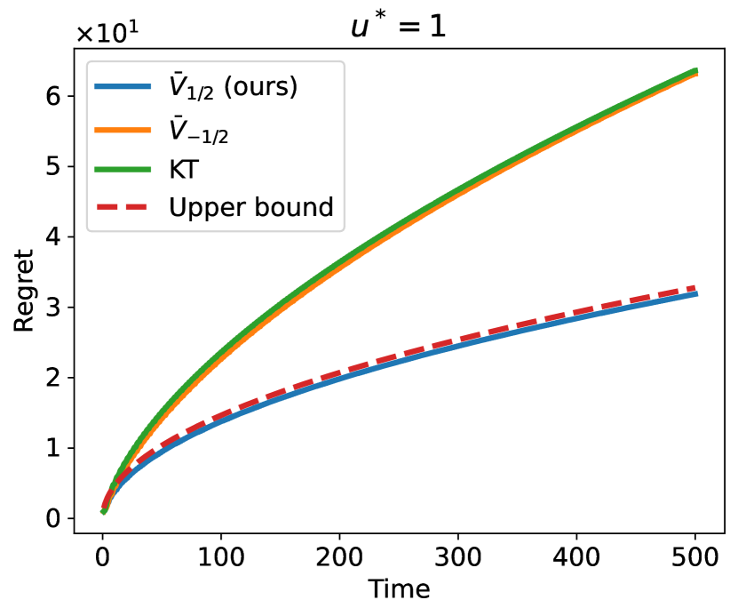
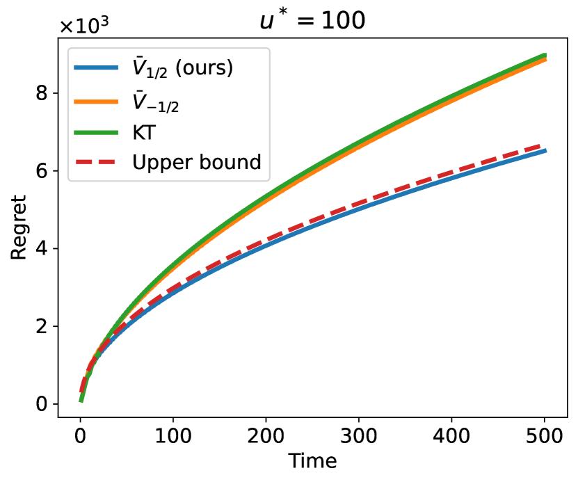
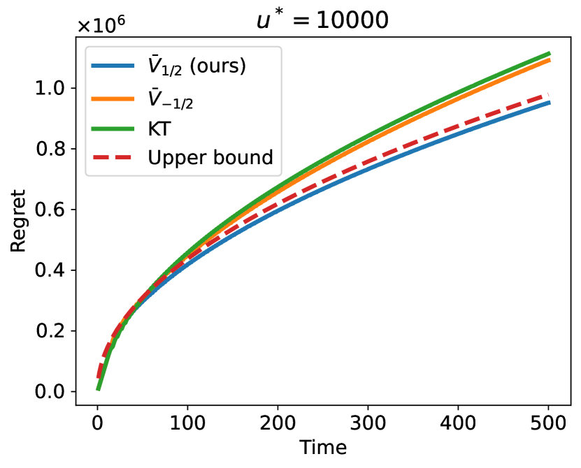
Figure 2: More cases of $u^{*}$ to support Figure 1(a); $C=1$, $T=500$.

The effect of $T$

Next, we investigate the effect of the maximum time horizon $T$. When closely comparing the regret upper bounds of the two potential-based algorithms (Theorem 4 and 11), one can see that for all fixed $C$ and nonzero $u^{*}$, the upper bound based on the new potential $\bar{V}_{1/2}$ is always better if $T$ is long enough ($O(\sqrt{T})$ as opposed to $O(\sqrt{T\log T})$). Then, a reasonable guess is that for some small $u^{*}$, the performance of our algorithm may be weaker than the baselines at $T=500$ (Figure 2), but better than the baselines at larger $T$. Such a guess is true in certain cases, as shown in Figure 3. Specifically, we pick $u^{*}=0.3$ and vary the maximum $T$. Initially our algorithm is worse, but as $T$ increases it can still outperform the baselines.

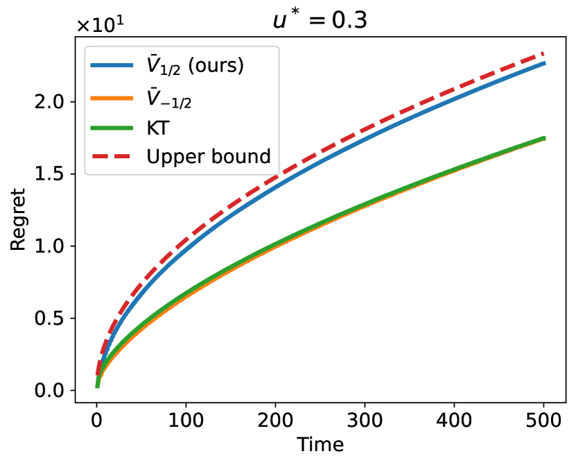
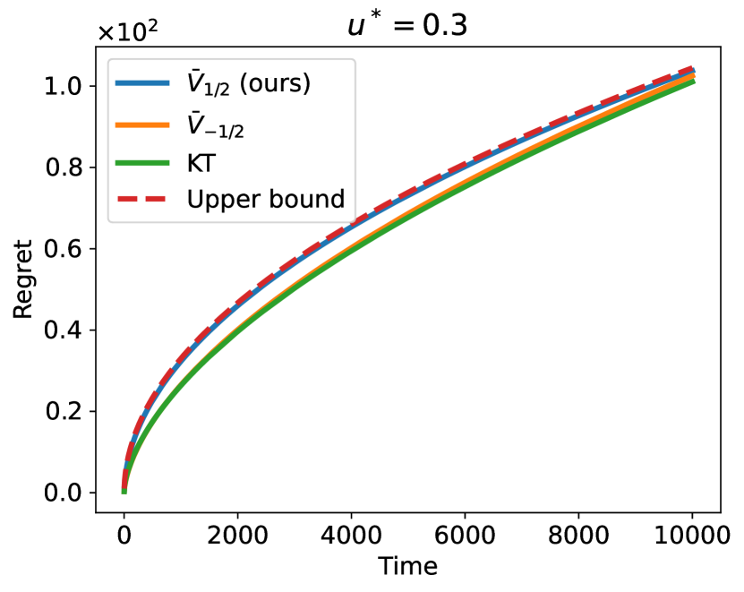
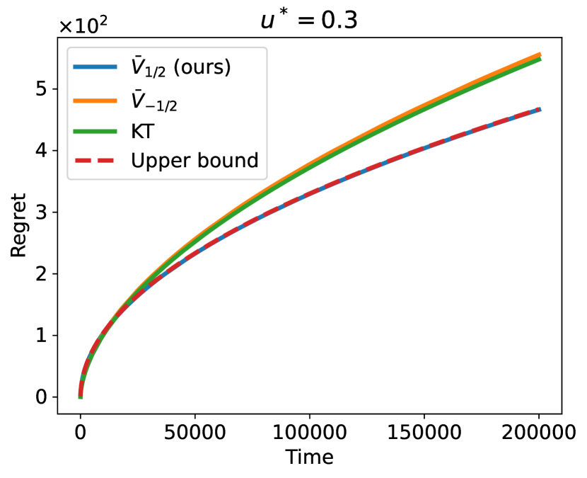
Figure 3: One-dimensional task with $C=1$ and $u^{*}=0.3$. From left to right: $T=500,10000,200000$.

A different hyperparameter $C$

Finally, we investigate the effect of the hyperparameter $C$ on the qualitative comparison of the three algorithms. We change $C$ to 10 and present results parallel to Figure 2 in Figure 4. The initial wealth of KT is scaled accordingly to $10\sqrt{e}$.

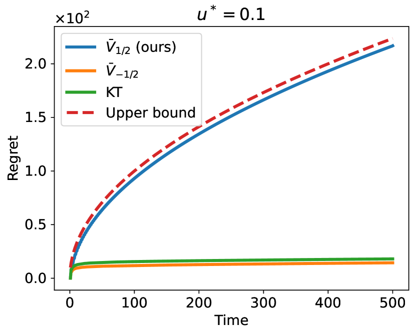
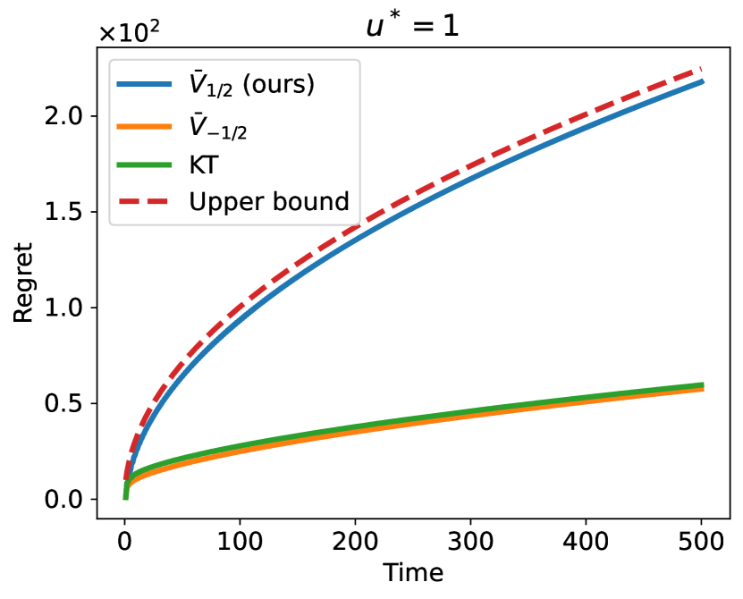
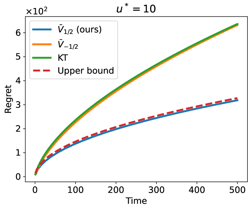
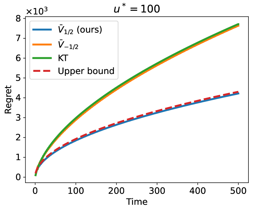
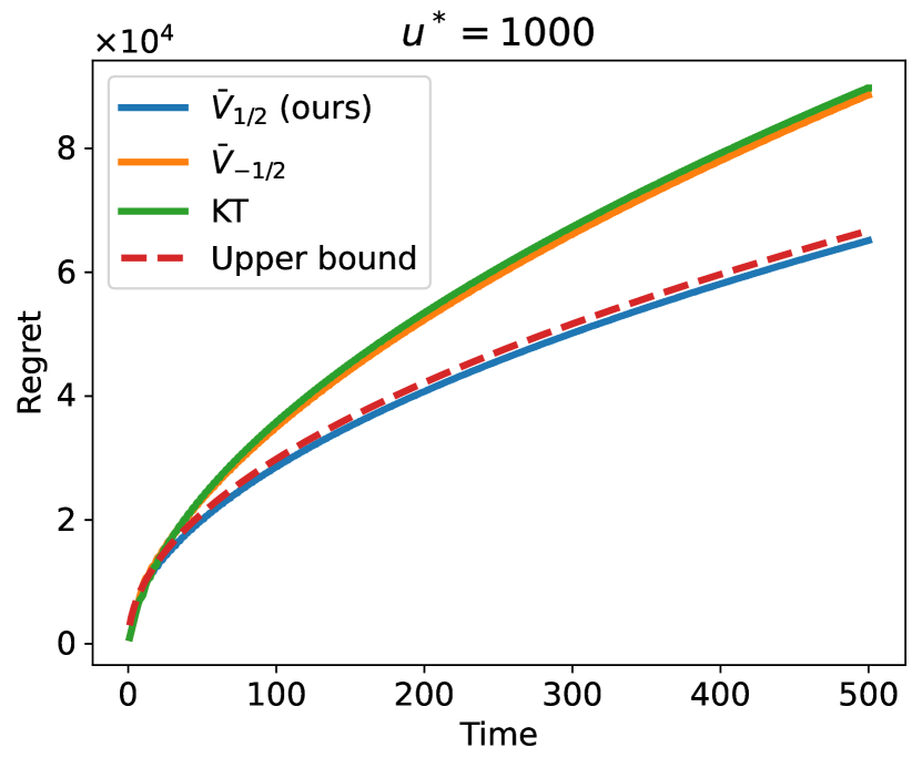
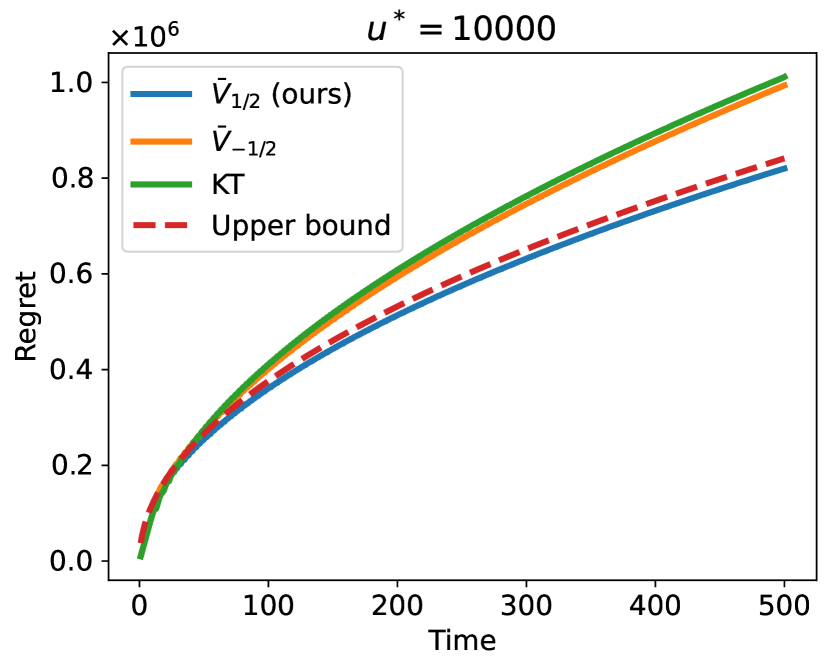
Figure 4: One-dimensional task with $C=10$.

Figure 4 exhibits a similar behavior as Figure 2: while sacrificing the regret at small $|u^{*}|$, our algorithm is better when $u^{*}$ is far-away. However, we also see that our algorithm exhibits less qualitative improvement over the baselines: in order to beat our algorithm (at $T=500$), previously (with $C=1$) the baselines should initialize at $\tilde{u}$ with error $|\tilde{u}-u^{*}|\leq 1$, but now (with $C=10$) such an error is allowed to be less than 10. A possible concern is that the advantage of our algorithm becomes harder to justify in this setting. We address this concern from three different perspectives.

1. Even with $C=10$, our algorithm still outperforms the baselines when $u^{*}$ is everywhere except on a compact set. Therefore, our algorithm still works better in more situations (of $u^{*}$).

2. Theoretically, for all fixed $C$ and nonzero $u^{*}$, our algorithm always guarantees better regret bound than the baselines when $T$ is large enough. Empirically this is validated in Figure 3.

3. The key idea of parameter-free algorithms is to use a simple hyperparameter to replace the laborious tuning of learning rates. In practice (e.g., [37, 10]), such a hyperparameter is often simply set to 1, and the resulting algorithms already exhibit strong empirical performance. Actually, changing $C$ amounts to trading off loss with regret; without any prior knowledge, the most natural choice is perhaps $C=1$. Therefore, when our algorithm and the two baselines are in the most natural configuration, our algorithm has the best performance unless a very accurate guess of $u^{*}$ is known a priori (Figure 2).

D.4 Additional experiment: 1D OLO with stochastic loss

As suggested by an anonymous reviewer, we now consider another one-dimensional experimental setting where loss gradients are iid stochastic, rather than generated from linearization. We choose $C=1$ and $T=500$; the loss gradients $g_{t}$ are generated iid on the support $\{\pm 1\}$, with mean $0.2$. Each algorithm is run 50 times, and the mean of the negative cumulative loss $-\sum_{t=1}^{T}g_{t}x_{t}$ as a function of $T$ is plotted in Figure 5; higher is better. Our algorithm beats both baselines in this setting.

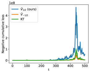
Figure 5: 1D OLO with stochastic losses. The plot shows the negative cumulative loss as a function of $T$; higher is better.

D.5 Additional experiment: High-dimensional regression with real data

In the last subsection, we report a high-dimensional regression experiment with real data. We use the YearPredictionMSD dataset [8] available from the UCI Machine Learning Repository [17], and the context of this dataset is to predict the release year of a song from its audio features. The raw data is preprocessed in two steps.

1. Feature normalization. For all the features (columns of the data matrix), we perform min-max scaling to transform their range to $[0,1]$.

2. Row scaling. For all the feature vectors (rows of the data matrix, i.e., training samples), we scale them such that each feature vector has $L_{2}$-norm 1. This is due to the Lipschitz requirement in our setting, and the same procedure has been performed in prior works (e.g., [37]).

After that, we use a linear model with absolute loss $l_{t}(x)=|\left\langle z_{t},x\right\rangle-y_{t}|$, where $z_{t}\in\mathbb{R}^{90}$ and $y_{t}\in\mathbb{R}_{+}$ are the $t$-th sampled feature vector and target. This can be converted into a 90-dimensional unconstrained OLO problem: the adversary picks $g_{t}=z_{t}$ if $\left\langle z_{t},x_{t}\right\rangle\geq y_{t}$, while $g_{t}=-z_{t}$ otherwise. Same as before, we consider three algorithms with $C=1$: ($i$) Algorithm 4 constructed from $\bar{V}_{1/2}$; ($ii$) Algorithm 4 constructed from $\bar{V}_{-1/2}$; and ($iii$) KT.

To study how these algorithms adapt to the distance to the optimal comparator, we use a parameter $\gamma$ to scale the target $y_{t}$. That is, we assign $y_{t}\leftarrow\gamma y_{t}$, and $\gamma$ is varied across different settings. Due to the linearity of our regression model, the optimal comparator is effectively scaled by $\gamma$. With a small $\gamma$, the comparators are brought closer to our initialization $0$. Note that such a scaling does not work if we use a nonlinear regression model. In those general cases, one may only care about the unscaled setting ($\gamma=1$).

Our results are presented in two ways, ($i$) fix $\gamma$ and vary $T$; ($ii$) fix $T$ and vary $\gamma$. Specifically, since $(z_{t},y_{t})$ is sampled from the dataset, in each setting (of $\gamma$) we run each algorithm 5 times and use the average cumulative OCO loss $\sum_{t=1}^{T}l_{t}(x_{t})$ as the “TotalLoss” of this algorithm. Figure 6 shows the type-($i$) results where we fix $\gamma$ at different values and plot TotalLoss as a function of $T$.

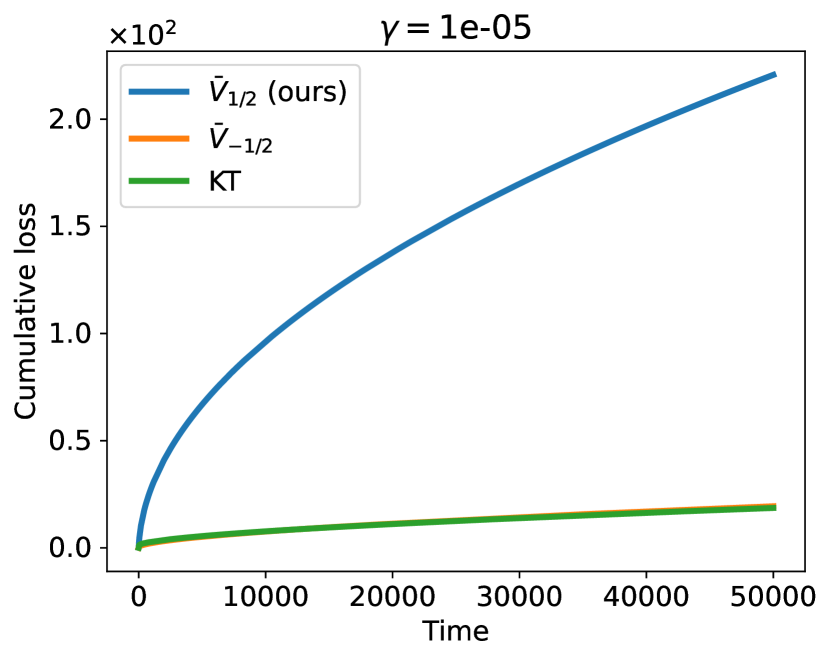
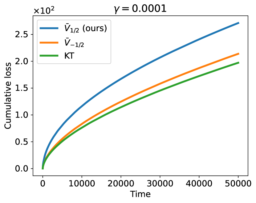
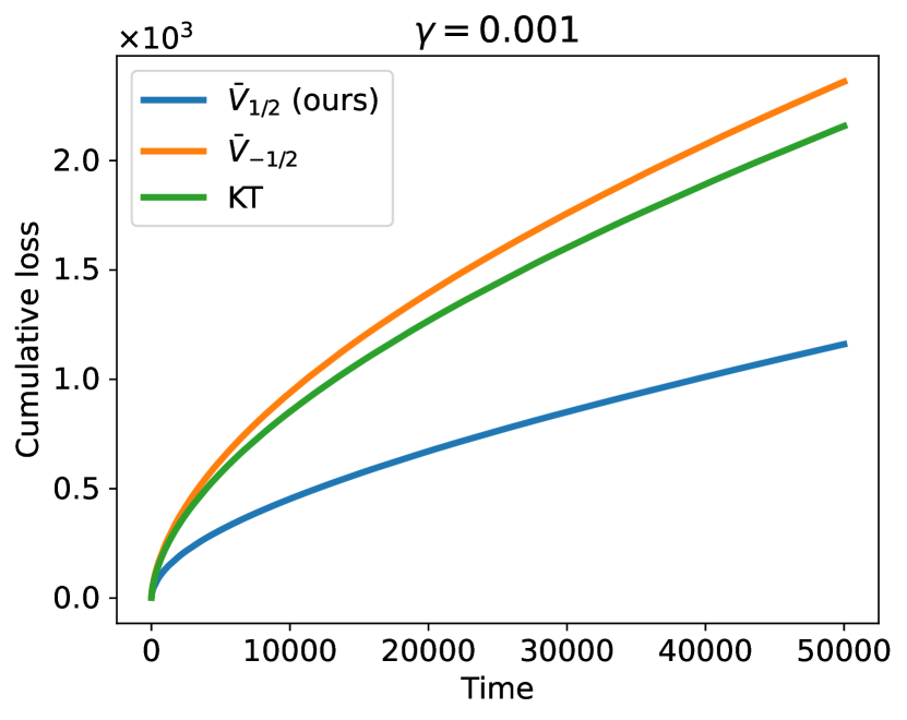
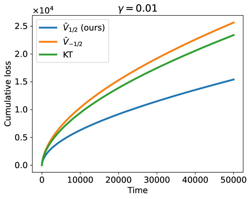
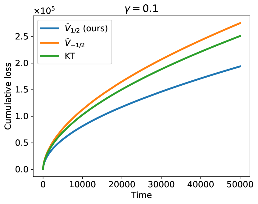
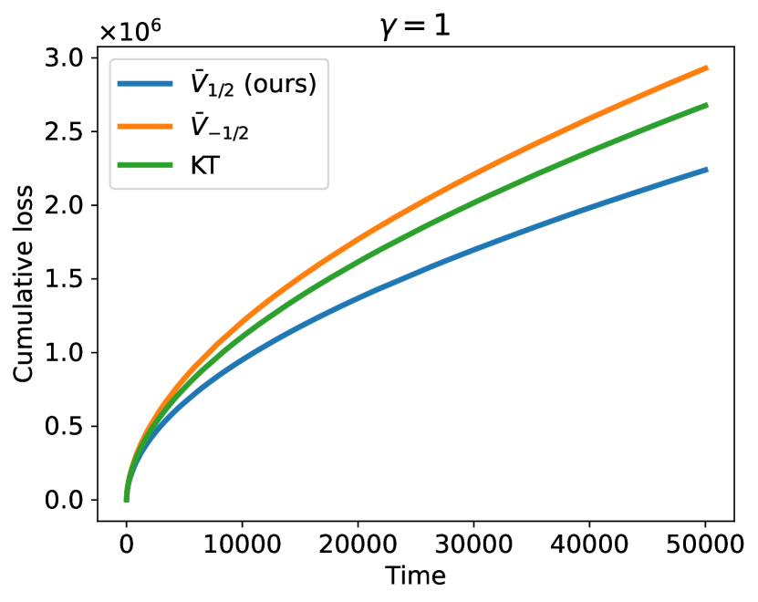
Figure 6: High-dimensional experiment with real data. $C=1$.

As for the type-($ii$) results, Figure 7 shows the difference between KT and our algorithm ($\textrm{TotalLoss}|_{KT}-\textrm{TotalLoss}|_{ours}$) as a function of $\gamma$. In other words, it plots the difference between the green and blue lines in Figure 6 at $T=50000$.

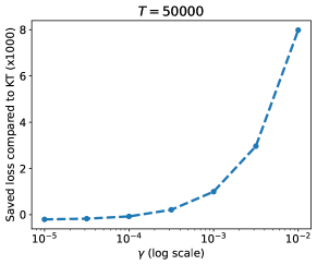
Figure 7: High-dimensional regression. Plot shows the TotalLoss of KT minus the TotalLoss of our algorithm.

Combining two figures, we can draw a similar conclusion as the one-dimensional experiment: our algorithm outperforms the baseline when the optimal comparator is far-away from the initial prediction.

References

- AHR [08] Jacob Abernethy, Elad E Hazan, and Alexander Rakhlin. Competing in the dark: An efficient algorithm for bandit linear optimization. In Conference on Learning Theory, pages 263–273, 2008.
- AP [13] Alexandr Andoni and Rina Panigrahy. A differential equations approach to optimizing regret trade-offs. arXiv preprint arXiv:1305.1359, 2013.
- AWH [13] George B Arfken, Hans J Weber, and Frank E Harris. Mathematical Methods for Physicists: A Comprehensive Guide. Academic Press, 2013.
- Ber [12] Dimitri Bertsekas. Dynamic programming and optimal control: Volume I. Athena scientific, 2012.
- [5] Erhan Bayraktar, Ibrahim Ekren, and Xin Zhang. Finite-time 4-expert prediction problem. Communications in Partial Differential Equations, 45(7):714–757, 2020.
- [6] Erhan Bayraktar, Ibrahim Ekren, and Yili Zhang. On the asymptotic optimality of the comb strategy for prediction with expert advice. The Annals of Applied Probability, 30(6):2517–2546, 2020.
- BEZ [21] Erhan Bayraktar, Ibrahim Ekren, and Xin Zhang. Prediction against a limited adversary. Journal of Machine Learning Research, 22(72):1–33, 2021.
- BMEWL [11] Thierry Bertin-Mahieux, Daniel P.W. Ellis, Brian Whitman, and Paul Lamere. The million song dataset. In ISMIR 2011, 2011.
- BPZ [20] Erhan Bayraktar, H Vincent Poor, and Xin Zhang. Malicious experts versus the multiplicative weights algorithm in online prediction. IEEE Transactions on Information Theory, 67(1):559–565, 2020.
- CLO [22] Keyi Chen, John Langford, and Francesco Orabona. Better parameter-free stochastic optimization with ode updates for coin-betting. In Proceedings of the AAAI Conference on Artificial Intelligence, 2022.
- CO [18] Ashok Cutkosky and Francesco Orabona. Black-box reductions for parameter-free online learning in banach spaces. In Conference on Learning Theory, pages 1493–1529, 2018.
- Cov [66] Thomas M Cover. Behavior of sequential predictors of binary sequences. Technical report, Stanford University, 1966.
- [13] Ashok Cutkosky. Artificial constraints and hints for unbounded online learning. In Conference on Learning Theory, pages 874–894. PMLR, 2019.
- [14] Ashok Cutkosky. Combining online learning guarantees. In Conference on Learning Theory, pages 895–913. PMLR, 2019.
- Cut [20] Ashok Cutkosky. Parameter-free, dynamic, and strongly-adaptive online learning. In International Conference on Machine Learning, pages 2250–2259. PMLR, 2020.
- DC [22] Nadejda Drenska and Jeff Calder. Online prediction with history-dependent experts: the general case. Communications on Pure and Applied Mathematics, 2022.
- DG [17] Dheeru Dua and Casey Graff. UCI machine learning repository, 2017.
- [18] Nadejda Drenska and Robert V Kohn. A PDE approach to the prediction of a binary sequence with advice from two history-dependent experts. arXiv preprint arXiv:2007.12732, 2020.
- [19] Nadejda Drenska and Robert V Kohn. Prediction with expert advice: A PDE perspective. Journal of Nonlinear Science, 30(1):137–173, 2020.
- DM [19] Amit Daniely and Yishay Mansour. Competitive ratio vs regret minimization: achieving the best of both worlds. In Algorithmic Learning Theory, pages 333–368. PMLR, 2019.
- FRS [18] Dylan J Foster, Alexander Rakhlin, and Karthik Sridharan. Online learning: Sufficient statistics and the burkholder method. In Conference On Learning Theory, pages 3028–3064. PMLR, 2018.
- Gor [41] Robert D Gordon. Values of mills’ ratio of area to bounding ordinate and of the normal probability integral for large values of the argument. The Annals of Mathematical Statistics, 12(3):364–366, 1941.
- HLPR [20] Nicholas JA Harvey, Christopher Liaw, Edwin A Perkins, and Sikander Randhawa. Optimal anytime regret for two experts. In IEEE 61st Annual Symposium on Foundations of Computer Science, pages 1404–1415. IEEE, 2020.
- JO [19] Kwang-Sung Jun and Francesco Orabona. Parameter-free locally differentially private stochastic subgradient descent. In Workshop on Privacy in Machine Learning at NeurIPS’19, 2019.
- Kj [56] JL Kelly jr. A new interpretation of information rate. The Bell System Technical Journal, 1956.
- [26] Vladimir A Kobzar, Robert V Kohn, and Zhilei Wang. New potential-based bounds for prediction with expert advice. In Conference on Learning Theory, pages 2370–2405, 2020.
- [27] Vladimir A Kobzar, Robert V Kohn, and Zhilei Wang. New potential-based bounds for the geometric-stopping version of prediction with expert advice. In Mathematical and Scientific Machine Learning, pages 537–554, 2020.
- Kle [13] Achim Klenke. Probability theory: a comprehensive course. Springer Science & Business Media, 2013.
- KP [11] Michael Kapralov and Rina Panigrahy. Prediction strategies without loss. Advances in Neural Information Processing Systems, 24, 2011.
- KS [12] Victor Korolev and Irina Shevtsova. An improvement of the berry–esseen inequality with applications to poisson and mixed poisson random sums. Scandinavian Actuarial Journal, 2012(2):81–105, 2012.
- LW [94] Nick Littlestone and Manfred K Warmuth. The weighted majority algorithm. Information and Computation, 108(2):212–261, 1994.
- MA [13] Brendan McMahan and Jacob Abernethy. Minimax optimal algorithms for unconstrained linear optimization. Advances in Neural Information Processing Systems, 26:2724–2732, 2013.
- Mir [61] Willard L Miranker. A well posed problem for the backward heat equation. Proceedings of the American Mathematical Society, 12(2):243–247, 1961.
- MK [20] Zakaria Mhammedi and Wouter M Koolen. Lipschitz and comparator-norm adaptivity in online learning. In Conference on Learning Theory, pages 2858–2887, 2020.
- MO [14] H Brendan McMahan and Francesco Orabona. Unconstrained online linear learning in hilbert spaces: Minimax algorithms and normal approximations. In Conference on Learning Theory, pages 1020–1039, 2014.
- MS [12] Brendan Mcmahan and Matthew Streeter. No-regret algorithms for unconstrained online convex optimization. Advances in neural information processing systems, 25, 2012.
- OP [16] Francesco Orabona and Dávid Pál. Coin betting and parameter-free online learning. Advances in Neural Information Processing Systems, 29, 2016.
- Ora [13] Francesco Orabona. Dimension-free exponentiated gradient. In Advances in Neural Information Processing Systems, pages 1806–1814, 2013.
- Ora [19] Francesco Orabona. A modern introduction to online learning. arXiv preprint arXiv:1912.13213, 2019.
- OT [17] Francesco Orabona and Tatiana Tommasi. Training deep networks without learning rates through coin betting. Advances in Neural Information Processing Systems, 30:2160–2170, 2017.
- Pay [75] Lawrence Edward Payne. Improperly posed problems in partial differential equations. SIAM, 1975.
- Roc [15] Ralph Tyrell Rockafellar. Convex analysis. Princeton university press, 2015.
- Rok [17] Dmitry B Rokhlin. PDE approach to the problem of online prediction with expert advice: a construction of potential-based strategies. arXiv preprint arXiv:1705.01091, 2017.
- RSS [12] Sasha Rakhlin, Ohad Shamir, and Karthik Sridharan. Relax and randomize: From value to algorithms. Advances in Neural Information Processing Systems, 25:2141–2149, 2012.
- SS [11] Shai Shalev-Shwartz. Online learning and online convex optimization. Foundations and trends in Machine Learning, 4(2):107–194, 2011.
- vdH [19] Dirk van der Hoeven. User-specified local differential privacy in unconstrained adaptive online learning. Advances in Neural Information Processing Systems, 32, 2019.
- ZCP [22] Zhiyu Zhang, Ashok Cutkosky, and Ioannis Paschalidis. Adversarial tracking control via strongly adaptive online learning with memory. In International Conference on Artificial Intelligence and Statistics, pages 8458–8492. PMLR, 2022.
- Zhu [14] Kangping Zhu. Two problems in applications of PDE. PhD thesis, New York University, 2014.
- Zin [03] Martin Zinkevich. Online convex programming and generalized infinitesimal gradient ascent. In International Conference on Machine Learning, pages 928–936, 2003.