Fermi polarons at finite temperature: Spectral function and rf-spectroscopy

Abstract

We present a systematic study of a mobile impurity immersed in a three-dimensional Fermi sea of fermions at finite temperature, by using the standard non-self-consistent many-body $T$-matrix theory that is equivalent to a finite-temperature variational approach with the inclusion of one-particle-hole excitation. The impurity spectral function is determined in the real-frequency domain, avoiding any potential errors due to the numerical analytic continuation in previous $T$-matrix calculations and the small spectral broadening parameter used in variational calculations. In the weak-coupling limit, we find that the quasiparticle decay rate of both attractive and repulsive polarons does not increase significantly with increasing temperature, and therefore Fermi polarons may remain well-defined far above Fermi degeneracy. In contrast, near the unitary limit with strong coupling, the decay rate of Fermi polarons rapidly increase and the quasiparticle picture breaks down close to the Fermi temperature. We analyze in detail the recent ejection and injection radio-frequency (rf) spectroscopy measurements, performed at Massachusetts Institute of Technology (MIT) and at European Laboratory for Non-Linear Spectroscopy (LENS), respectively. We show that the momentum average of the spectral function, which is necessary to account for the observed rf-spectroscopy, has a sizable contribution to the width of the quasiparticle peak in spectroscopy. As a result, the measured decay rate of Fermi polarons could be significantly larger than the calculated quasiparticle decay rate at zero momentum. By take this crucial contribution into account, we find that there is a reasonable agreement between theory and experiment for the lifetime of Fermi polarons in the strong-coupling regime, as long as they remain well-defined.

I Introduction

The polaron problem that describes a single impurity interacting with a host environment is a long-lasting research topic in modern physics Alexandrov2010 . The initial study can be traced back to the seminal work by Landau on the description of electron motion in crystal lattices Landau1933 . The resulting quasiparticle picture plays a fundamental role in understanding the complex quantum many-body physics, occurring in solid state systems Mahan1967 ; Roulet1969 ; Nozieres1969 , helium liquids Bardeen1967 and most recently in ultracold atomic quantum gases Massignan2014 ; Lan2014 ; Schmidt2018 . The latest development with ultracold atoms is particularly exciting, since highly imbalanced quantum mixtures present a clean and controllable test-bed that is well-suited to explore the limits of Landau’s quasiparticle paradigm. In the extremely imbalanced case, the minority component of mixtures realizes the single-impurity limit, and the interaction between the impurity and surrounding environment (i.e., the majority component) can be precisely tuned to be arbitrarily strong, by using the so-called Feshbach resonance technique Bloch2008 ; Chin2010 . As a result, one can systematically investigate the polaron physics with unprecedented precision in the strong-coupling regime Massignan2014 ; Lan2014 ; Schmidt2018 .

The rapid growing interest on the ultracold atomic polaron physics already leads to a number of breakthrough experimental discoveries over the past fifteen years Schirotzek2009 ; Zhang2012 ; Kohstall2012 ; Koschorreck2012 ; Cetina2016 ; Hu2016 ; Jorgensen2016 ; Scazza2017 ; Zan2019 ; Zan2020 ; Ness2020 , inspired by the celebrated Chevy’s variational ansatz for Fermi polarons, which describes the dressing of the impurity motion with one particle-hole excitation of the host Fermi sea Chevy2006 . The ground-state attractive Fermi polarons was first realized with ⁶Li atoms in 2009 at Massachusetts Institute of Technology (MIT) Schirotzek2009 , by using the ejection radio-frequency (rf) spectroscopy through the measurement of the transferring rate of the impurity to a third, unoccupied hyperfine state. In 2012, novel excited state of repulsive Fermi polarons was subsequently observed Kohstall2012 ; Koschorreck2012 . Measurements have also extended to Bose polarons in 2016 Hu2016 ; Jorgensen2016 , where the host environment is given by a weakly interacting Bose-Einstein condensate. Those milestone experiments motivated numerous theoretical works Combescot2007 ; Prokofev2008 ; Punk2009 ; Cui2010 ; Massignan2011 ; Schmidt2012 ; Parish2013 ; Vlietinck2013 ; Rath2013 ; PenaArdila2015 ; Levinsen2015 ; Goulko2016 ; Hu2018 ; Tajima2018 ; Tajima2019 ; PenaArdila2019 ; Mulkerin2019 ; Liu2019 ; Wang2019 ; Liu2020 ; Adlong2020 ; Parish2021 ; Pessoa2021 ; Hu2021 .

For Fermi polarons, most of the theoretical studies focus on the idealized case of zero temperature. This is reasonable, since the experiments were mostly carried out at low temperatures, where the finite-temperature effect could be negligible. However, Fermi polarons at nonzero temperature are also of great interest, particularly in the strong-coupling regime. In a recent experiment at MIT Zan2019 , the temperature evolution of the rf spectroscopy of unitary Fermi polarons with infinitely large coupling constant right on Feshbach resonance was measured up to two times Fermi temperature, $2T_{F}$. The breakdown of polaron quasiparticle near Fermi degeneracy was clearly demonstrated.

On the theoretical side, finite-temperature quasiparticle properties of Fermi polarons are less understood. The first theoretical investigation of finite-temperature Fermi polarons by the present authors and co-workers is restricted to the low-temperature regime (i.e., $T<0.2T_{F}$) Hu2018 , where the quasiparticle properties such as the decay rate are extracted from the finite-temperature Green function of the impurity, by treating the smallest fermionic Matsubara frequency (in absolute magnitude) $\pi k_{B}T$ as a small parameter. This restriction can be lifted, either by directly using a retarded Green function in the real-frequency domain Mulkerin2019 , or by applying the analytic continuation to convert the Matsubara frequency to real frequency Tajima2018 ; Tajima2019 . The latter may suffer from some uncontrollable errors, since, strictly speaking, the numerical analytic continuation is not a well-defined procedure Goulko2016 ; Haussmann2009 . Alternatively, an interesting finite-temperature variational approach has recently been proposed by Meera Parish and her collaborators Liu2019 ; Liu2020 ; Parish2021 . By solving the Chevy ansatz (extended to finite temperature) at the level of one-particle-hole excitation and keeping a sufficiently large number of discrete eigenstates Liu2019 , both short-time dynamics and rf-spectroscopy of Fermi polarons at finite temperature have been investigated in detail. However, the finite-temperature quasiparticle properties of Fermi polarons over a wide temperature regime has not been addressed, probably due to the difficulty of reaching the continuous limit, where an infinitely large number of truncated basis is needed.

In this work, we aim to present a systematic study of quasiparticle properties of both attractive and repulsive Fermi polarons, by using the conventional non-self-consistent many-body $T$-matrix theory in the single-impurity limit Combescot2007 ; Massignan2011 . The theory is fully equivalent to the finite-temperature variational approach Liu2019 ; Parish2021 , but has the advantage and simplicity of avoiding a small spectral broadening parameter, which might be needed in the calculations of spectral function and spectroscopy. As we work directly in the real-frequency domain, our calculations are also free from any potential errors arising from the numerical analytic continuation. Our main results can be briefly summarized as follows.

First, we present a detailed study of the impurity spectral function, from which we extract the finite-temperature decay rate or lifetime of Fermi polarons. We find somehow surprisingly that, with a weak coupling strength between the impurity and the Fermi sea (i.e., $1/(k_{F}a)\leq-1$ for attractive polarons and $1/(k_{F}a)\geq 1$ for repulsive polarons), the decay rate of both attractive and repulsive Fermi polarons at zero momentum does not increases significantly at high temperature, indicating the existence a well-defined quasiparticle far above the Fermi degeneracy. In sharp contrast, in the strong-coupling limit, the lifetime of Fermi polarons rapidly increases with increasing temperature, and in the unitary limit the quasiparticle picture of Fermi polarons already breaks down near Fermi degeneracy. This observation agrees well with our previous $T$-matrix results on the width of quasiparticle peak in the ejection rf-spectroscopy Mulkerin2019 .

On the other hand, by utilizing the single-impurity limit, we can now calculate the impurity spectral function in a more efficient way, much faster than that in our previous work Mulkerin2019 , which was carried out at finite impurity density and has a bottleneck in the impurity self-energy calculation with real-frequency. The consideration of the single-impurity limit is also more physical, as we are interested in the single-polaron problem, and the polaron-polaron interaction at finite density then should be irrelevant and should be avoided. Taking the advantage of a fast calculation of the spectral function, we are able to carefully examine the ejection and injection rf-spectroscopy. As the rf-spectroscopies of Fermi polarons in recent experiments Scazza2017 ; Zan2019 are not momentum-resolved, we pay specific attentions to the possible effect of the momentum average on the measured width of the quasiparticle peak in the spectra. We find that the measured width is typically much larger than the decay rate of Fermi polarons at zero momentum, according to our theoretical simulations.

For the finite-temperature measurement of unitary Fermi polarons at MIT Zan2019 , we find a good agreement between theory and experiment below a characteristic temperature $T<0.7T_{F}$, without any free parameters. Above this temperature, the quasiparticle picture starts to break down and our non-self-consistent $T$-matrix approach (or finite-temperature Chevy ansatz with one-particle-hole excitation) is not able to capture the key physics. A refined theoretical treatment is therefore needed. For the low-temperature measurement of repulsive Fermi polarons at European Laboratory for Non-Linear Spectroscopy (LENS) Scazza2017 , we show that the decay rate determined from Rabi oscillations cannot be theoretically explained solely by considering the decay rate of zero-momentum repulsive polarons even at nonzero temperature Adlong2020 . It can be quantitatively understood, only when we take into account the momentum average in the impurity spectral function.

The rest of the manuscript is organized in the following way. In Sec. II, we briefly describe the non-self-consistent $T$-matrix approach for a single Fermi polaron at finite temperature. In Sec. III, we discuss in detail the impurity spectral function and the associated quasiparticle decay rate, as functions of temperature and coupling strength. In Sec. IV and Sec. V, we consider the ejection and injection rf-spectroscopies, respectively. We compare our theoretical predictions with the measurements at MIT and LENS, without adjustable parameters. We comment briefly on how to further improve the theoretical description of Fermi polarons, by going beyond the simple $T$-matrix approach. In Sec. VI, we consider the cases with unequal mass between the impurity and the host environment. In Sec. VII, we summarize the results. Finally, in Appendix A we present some subtle details of our numerical calculations.

II The non-self-consistent T-matrix approach for a single impurity

We consider an impurity of mass $m_{I}$ interacting with a homogeneous bath of fermionic atoms of mass $m$ in three dimensions, as described by the model Hamiltonian (the system volume is set to unity, $V=1$),

$$\mathcal{H}=\sum_{\mathbf{k}}\epsilon_{\mathbf{k}}c_{\mathbf{k}}^{\dagger}c_{\mathbf{k}}+\sum_{\mathbf{p}}\epsilon_{\mathbf{p}}^{(I)}d_{\mathbf{p}}^{\dagger}d_{\mathbf{p}}+g\sum_{\mathbf{kpq}}c_{\mathbf{k}}^{\dagger}d_{\mathbf{q}-\mathbf{k}}^{\dagger}d_{\mathbf{p}}c_{\mathbf{q}-\mathbf{p}},$$ (1)

where $c_{\mathbf{k}}^{\dagger}$ and $d_{\mathbf{p}}^{\dagger}$ are the creation field operators for fermionic atoms and the impurity, respectively. The first two terms in the Hamiltonian are the single-particle terms with dispersion relation $\epsilon_{\mathbf{k}}=\hbar^{2}\mathbf{k}^{2}/(2m)$ and $\epsilon_{\mathbf{p}}^{(I)}=\hbar^{2}\mathbf{p}^{2}/(2m_{I})$, while the last term describes the $s$-wave contact interaction with a bare coupling strength $g$. It is well-known that the use of the contact interaction potential is not physical at high energy, and the associated ultraviolet divergence could be removed by using the standard regularization relation,

$$\frac{1}{g}=\frac{m_{r}}{2\pi\hbar^{2}a}-\sum_{\mathbf{p}}\frac{2m_{r}}{\hbar^{2}\mathbf{p}^{2}},$$ (2)

which replaces the bare interaction strength $g$ with the $s$-wave scattering length $a$. Here, $m_{r}\equiv mm_{I}/(m+m_{I})$ is the reduced mass.

In the single-impurity limit, the model Hamiltonian can be conveniently solved by the non-self-consistent $T$-matrix theory Combescot2007 , where the motion of the impurity is described by ladder diagrams, accounting for the successive forward scatterings between the impurity and fermions in the particle-particle channel. This gives rise to the inverse two-particle vertex function at nonzero temperature $T$,

$$\Gamma^{-1}\left(\mathcal{Q}\right)=\frac{1}{g}+\sum_{\mathcal{K}}\mathcal{G}\left(\mathcal{K}\right)G_{0}\left(\mathcal{Q}-\mathcal{K}\right),$$ (3)

where $\mathcal{K}\equiv(\mathbf{k},i\omega_{m})$ and $\mathcal{Q}\equiv(\mathbf{q},i\nu_{n})$ are the short-hand notations for momentum ($\mathbf{k}$ or $\mathbf{q}$) and Matsubara frequency ($\omega_{m}=(2m+1)\pi k_{B}T$ or $\nu_{n}=2n\pi k_{B}T$ with integers $m$ and $n$), $\sum_{\mathcal{K}}\equiv k_{B}T\sum_{i\omega_{m}}\sum_{\mathbf{k}}$ and $\sum_{\mathcal{Q}}\equiv k_{B}T\sum_{i\nu_{n}}\sum_{\mathbf{q}}$, and

$$\mathcal{G}\mathcal{\left(K\right)}=\frac{1}{i\omega_{m}-\epsilon_{\mathbf{k}}+\mu}=\frac{1}{i\omega_{m}-\xi_{\mathbf{k}}}$$ (4)

and

$$G_{0}\mathcal{\left(Q-K\right)}=\frac{1}{i\nu_{n}-i\omega_{m}-\epsilon_{\mathbf{q}-\mathbf{k}}^{(I)}}$$ (5)

are the finite-temperature Green functions for fermionic atoms and the impurity, respectively.

In the single-impurity case, the Green function of atoms is barely affected, so it takes the standard non-interacting form with a (temperature-dependent) chemical potential $\mu(T)$. Instead, the impurity Green function will be strongly renormalized by the impurity-atom coupling. However, in the non-self-consistent $T$-matrix approach we take its non-interacting form. This is because, there is a cancellation between the self-energy renormalization of the impurity Green function and the vertex correction to $\Gamma(\mathcal{Q})$ Mahan1967 ; Roulet1969 ; Nozieres1969 . If we wish to use the impurity Green function in a self-consistent way, we may then need to simultaneously take into account the vertex correction, which is beyond the scope of this work. Otherwise, the approximate theory may become worse. This explains why at zero temperature we can obtain a very accurate (attractive) polaron energy within the non-self-consistent $T$-matrix theory (or equivalently within Chevy’s variational approach) Combescot2007 . We note also that, with a single impurity, the quantum statistics of the impurity is irrelevant. Here, for concreteness we consider fermionic impurities, in connection with the recent experiments Scazza2017 ; Zan2019 . Therefore, in the two-particle vertex function $\Gamma(\mathcal{Q})$ we use bosonic Matsubara frequencies $\nu_{n}=2n\pi k_{B}T$ ($n\in\mathbb{Z}$).

Given the free Green functions $\mathcal{G}(\mathcal{K})$ and $G_{0}(\mathcal{Q}-\mathcal{K})$ the Matsubara frequency summation in the vertex function $\Gamma(\mathcal{Q})$ over $i\omega_{m}$ is easy to evaluate. By replacing further the bare interaction strength $g$ with the scattering length $a$, we obtain Combescot2007 ,

$$\Gamma^{-1}\left(\mathcal{Q}\right)=\frac{m_{r}}{2\pi\hbar^{2}a}-\sum_{\mathbf{k}}\left[\frac{1-f\left(\xi_{\mathbf{k}}\right)}{i\nu_{n}-\xi_{\mathbf{k}}-\epsilon_{\mathbf{q}-\mathbf{k}}^{(I)}}+\frac{2m_{r}}{\hbar^{2}\mathbf{k}^{2}}\right],$$ (6)

where $f(x)\equiv 1/(e^{\beta x}+1)$ with $\beta\equiv 1/(k_{B}T)$ is the Fermi-Dirac distribution function. Here, we have discarded the distribution function related to the impurity, as the impurity chemical potential (which we do not show explicitly for convenience) tends to $-\infty$ at nonzero temperature. This treatment is also consistent with the fact that the quantum statistics of the impurity is not relevant.

We can now calculate the self-energy of the impurity $\Sigma(\mathcal{K})$ by winding back the out-going leg of fermionic atoms in the vertex function $\Gamma(\mathcal{Q})$ and connecting it with the in-coming leg for fermionic atoms. This physically describes the hole excitation and gives rise to,

$$\Sigma\mathcal{\left(K\right)}=\sum_{\mathcal{Q}}\Gamma\left(\mathcal{Q}\right)\frac{1}{i\nu_{n}-i\omega_{m}-\xi_{\mathbf{q}-\mathbf{k}}}.$$ (7)

To proceed, we can use the formal spectral representation of the vertex function, i.e.,

$$\Gamma\left(\mathcal{Q}\right)=\intop_{-\infty}^{\infty}\frac{d\Omega}{\pi}\frac{\left[-\textrm{Im}\Gamma_{R}\left(\mathbf{q},\Omega\right)\right]}{i\nu_{n}-\Omega},$$ (8)

where $\Gamma_{R}(\mathbf{q},\Omega)=\Gamma(\mathbf{q},i\nu_{n}\rightarrow\Omega+i0^{+})$ is the retarded vertex function after analytic continuation. The Matsubara frequency summation in the self-energy over $i\nu_{n}$ again is straightforward to evaluate. We find that,

$$\Sigma\mathcal{\left(K\right)}=\sum_{\mathbf{q}}\intop_{-\infty}^{\infty}\frac{d\Omega}{\pi}\left[-\textrm{Im}\Gamma_{R}\left(\mathbf{q},\Omega\right)\right]\frac{f\left(\xi_{\mathbf{q}-\mathbf{k}}\right)+f_{B}\left(\Omega\right)}{i\omega_{m}+\xi_{\mathbf{q}-\mathbf{k}}-\Omega},$$ (9)

where $f_{B}(\Omega)=1/(e^{\beta\Omega}-1)$ is the Bose-Einstein distribution function. In the single-impurity limit, the molecule occupation $f_{B}(\Omega)$ scales like $1/V$ and therefore is vanishingly small, in line with the infinitely negative impurity chemical potential as mentioned earlier. By removing $f_{B}\left(\Omega\right)$ in the above expression, we again use the spectral representation and finally arrive at Combescot2007 ,

$$\Sigma\mathcal{\left(K\right)}=\sum_{\mathbf{q}}f\left(\xi_{\mathbf{q}-\mathbf{k}}\right)\Gamma\left(\mathbf{q},i\omega_{m}+\xi_{\mathbf{q}-\mathbf{k}}\right).$$ (10)

The retarded interacting impurity Green function then takes the form,

$$G_{R}(\mathbf{k},\omega)=\frac{1}{\omega-\epsilon_{\mathbf{k}}^{(I)}-\Sigma_{R}(\mathbf{k},\omega)},$$ (11)

where the retarded self-energy $\Sigma_{R}(\mathbf{k},\omega)\equiv\Sigma(\mathbf{k},i\omega_{m}\rightarrow\omega+i0^{+})$. The pole position of the impurity Green function determines the (attractive or repulsive) polaron energy, i.e.,

$$\mathcal{E}_{P}\left(\mathbf{k}\right)=\epsilon_{\mathbf{k}}^{(I)}+\textrm{Re}\Sigma_{R}\left[\mathbf{k},\mathcal{E}_{P}\left(\mathbf{k}\right)\right].$$ (12)

By expanding the retarded self-energy near the zero momentum $\mathbf{k}=0$ and the polaron energy $\mathcal{E}_{P}\equiv\mathcal{E}_{P}\left(\mathbf{0}\right)$, we calculate directly various quasiparticle properties, including the polaron residue $\mathcal{Z}^{-1}=1-\partial\textrm{Re}\Sigma_{R}(0,\omega)/\partial\omega$, the effective mass $m_{*}/m_{I}=\mathcal{Z}^{-1}/[1+\partial\textrm{Re}\Sigma_{R}(\mathbf{k},\mathcal{E}_{P})/\partial\epsilon_{\mathbf{k}}^{(I)}]$, and also the polaron decay rate,

$$\Gamma=-2\mathcal{Z}\textrm{Im}\Sigma_{R}\left(\mathbf{0},\mathcal{E}_{P}\right).$$ (13)

For a nonzero decay rate, it corresponds to the full width at half maximum (FWHM) of the spectral function $A(\mathbf{k},\omega)\equiv-(1/\pi)\textrm{Im}G_{R}(\mathbf{k},\omega)$.

The set of equations, Eqs. (6), (10) and (11), constitute the well-documented non-self-consistent many-body $T$-matrix theory of Fermi polarons Massignan2014 ; Scazza2017 ; Combescot2007 . At zero temperature, its equivalence to Chevy’s variational ansatz is well-known from the seminal work Combescot2007 . At finite temperature, the equivalence to the finite-temperature variational approach proposed by Meera Parish and her co-workers has also been discussed Liu2019 .

II.1 Numerical calculations

The numerical solution of those coupled equations, however, is non-trivial, particularly at finite temperature. The calculation of the retarded self-energy at large frequency $\omega$ is subtle, due to the existence of the two-particle continuum. As we can see from Eq. (6), the integrand has infinite number of poles once $i\nu_{n}\rightarrow\Omega>\omega_{\textrm{th}}(\mathbf{q})=\min_{\mathbf{k}}\{\xi_{\mathbf{k}}+\epsilon_{\mathbf{q}-\mathbf{k}}^{(I)}\}$, where $\omega_{\textrm{th}}(\mathbf{q})$ is the threshold to enter the two-particle continuum at the momentum $\mathbf{q}$. We therefore need to take Cauchy principle value of the integral. This numerical difficulty does not arise in the finite-temperature variational approach Liu2019 ; Liu2020 ; Parish2021 , where one solves for the discretized variational wave-functions or parameters in momentum space. The discretization however would require a small broadening factor, in order to recover a continuous spectral function.

Alternatively, we can solve the coupled equations with Matsubara frequencies. This strategy has been used in our previous work at low temperature Hu2018 , where we can expand the impurity Green function, in terms of the small Matsubara frequency $\omega_{m}=(2m+1)k_{B}T$, in order to calculate the quasiparticle properties. At high temperature or in the calculation of the spectral function $A(\mathbf{k},\omega)$, one needs to numerically take the analytic continuation Tajima2018 ; Tajima2019 . Unfortunately, this procedure is not well-defined and may lead to uncontrollable uncertainties in the spectral function Goulko2016 ; Haussmann2009 .

In this work, we solve the coupled equations for the retarded impurity self-energy and Green function with real frequency, following the same idea in Ref. Mulkerin2019 , where the non-self-consistent $T$-matrix theory has been used to understand a Fermi polaron system at finite impurity density. The finite density makes the numerical calculations very time-consuming. For example, we have to keep the bosonic distribution function $f_{B}\left(\Omega\right)$ in Eq. (9) and hence have an additional integral over the frequency $\Omega$. As a result, one can hardly explore the finite temperature properties of Fermi polarons. Here, we take the advantage of the single-impurity limit and thereby greatly shorten the time needed for an accurate calculation of the spectral function. There is also no need to introduce any small broadening factor in the spectral function, allowing us to make a comparison of our theoretical predictions with the recent experiments Scazza2017 ; Zan2019 , without adjustable free parameters, as we shall see.

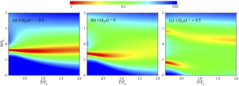
Figure 1: Two-dimensional contour plots of the temperature evolution of the zero-momentum impurity spectral function $A(\mathbf{k}=0,\omega$) at three dimensionless coupling strengths: $1/(k_{F}a)=-0.5$ (a), $0$ (b), and $+0.5$ (c). The spectral function is in units of $\varepsilon_{F}^{-1}$, where $\varepsilon_{F}\equiv\hbar^{2}k_{F}^{2}/(2m)$ is the Fermi energy. Each plot is shown in the logarithmic scale. We typically take the equal mass for the impurity and atoms, $m_{I}=m$, unless otherwise specified.

To be specific, we take the Fermi wave-vector $k_{F}\equiv(6\pi^{2}n)^{1/3}$ and Fermi energy $\varepsilon_{F}\equiv\hbar^{2}k_{F}^{2}/(2m)$ as the units of the momentum (or wave-vector) and energy, respectively. The temperature is then measured in units of the Fermi temperature $T_{F}=\varepsilon_{F}/k_{B}$. This choice corresponds to set $2m=\hbar=k_{B}=1$. We also define a mass ratio $-1<\alpha=(m_{I}-m)/(m_{I}+m)<1$, so $2m_{I}=(1+\alpha)/(1-\alpha)$ and the reduced mass $2m_{r}=(1+\alpha)/2$. The coupling between fermionic atoms and the impurity is characterized by a dimensionless interaction parameter $1/(k_{F}a)$. We then find that the dimensionless retarded two-particle propagator $\chi_{R}(\mathbf{q},\Omega)=\Gamma_{R}^{-1}(\mathbf{q},\Omega)$ can be written into the two-body and many-body parts (i.e., $\chi_{R}=\chi_{R}^{(2b)}+\chi_{R}^{(mb)}$),

$$\chi_{R}^{(2b)}\left(\mathbf{q},\Omega\right)=\frac{m_{r}}{2\pi\hbar^{2}a}-\sum_{\mathbf{k}}\left[\frac{1}{\Omega^{+}-\xi_{\mathbf{k}}-\epsilon_{\mathbf{q}-\mathbf{k}}^{(I)}}+\frac{2m_{r}}{\hbar^{2}\mathbf{k}^{2}}\right]=\frac{1+\alpha}{8\pi k_{F}a}+\frac{i\left(1+\alpha\right)^{3/2}}{8\sqrt{2}\pi}\sqrt{\Omega+\mu-\frac{\left(1-\alpha\right)}{2}q^{2}}$$ (14)

and

$$\chi_{R}^{(mb)}\left(\mathbf{q},\Omega\right)=\sum_{\mathbf{k}}\frac{f\left(\xi_{\mathbf{k}}\right)}{\Omega^{+}-\xi_{\mathbf{k}}-\epsilon_{\mathbf{q}-\mathbf{k}}^{(I)}}=\intop_{0}^{\infty}\frac{k^{2}dk}{2\pi^{2}}\intop_{-1}^{+1}\frac{dx}{2}\frac{f\left(k^{2}-\mu\right)}{\left(\Omega^{+}+\mu\right)-k^{2}-\left[\left(1-\alpha\right)/\left(1+\alpha\right)\right]\left(q^{2}+k^{2}-2qkx\right)},$$ (15)

where $\Omega^{+}\equiv\Omega+i0^{+}$ and $x\equiv\cos(\theta_{\mathbf{qk}})$, with $\theta_{\mathbf{qk}}$ being the angle between the vectors $\mathbf{q}$ and $\mathbf{k}$. In Appendix A, we list the detailed expressions for $\textrm{Im}\chi_{R}^{(mb)}$ and $\textrm{Re}\chi_{R}^{(mb)}$ and discuss their qualitative feature. Once the two-particle propagator $\chi_{R}(\mathbf{q},\Omega)$ is calculated, we take the inverse to obtain the real and imaginary parts of the two-particle vertex function $\Gamma_{R}(\mathbf{q},\Omega)$, which physically serves as the Green function of molecules. It is then straightforward to calculate the retarded self-energy,

$$\Sigma_{R}(\mathbf{k},\omega)=\intop_{0}^{\infty}\frac{q^{2}dq}{2\pi^{2}}\intop_{-1}^{+1}\frac{dx}{2}f\left(\xi_{\mathbf{q}-\mathbf{k}}\right)\Gamma_{R}\left(\mathbf{q},\omega+\xi_{\mathbf{q}-\mathbf{k}}\right),$$ (16)

where $\xi_{\mathbf{q}-\mathbf{k}}=q^{2}+k^{2}-2qkx-\mu$. This two-dimensional integral can be efficiently determined, if we take care of the possible pole in the two-particle vertex function, which corresponds to the two-body bound state that may arise in the strong-coupling regime when the scattering length is positive, $a>0$.

III Spectral function and quasiparticle lifetime

In this section, we discuss in detail the finite-temperature spectral function of Fermi polarons near a Feshbach resonance, in the case of equal mass $m_{I}=m$ (i.e., $\alpha=0$). We also present the quasiparticle properties of both attractive and repulsive polarons at arbitrary temperatures, extending our previous low-temperature results on attractive polarons Hu2018 . We emphasize that we do not use any small broadening factor in numerical calculations, so the quasiparticle decay rate obtained determines the intrinsic lifetime of Fermi polarons.

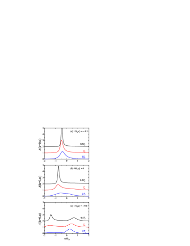
Figure 2: The impurity spectral function $A(\mathbf{k}=0,\omega$) at the dimensionless coupling strengths: $1/(k_{F}a)=-0.5$ (a), $0$ (b), and $+0.5$ (c). These curves are the cuts at three different temperatures (i.e., $T/T_{F}=0.5$, $1$, and $2$) in Fig. 1.

Fig. 1 presents the two-dimensional contour plots of the zero-momentum spectral function $A(\mathbf{k}=0,\omega$) as a function of temperature at the crossover from a Bardeen–Cooper–Schrieffer (BCS) superfluid to a Bose-Einstein condensate (BEC), where the dimensionless interaction parameter changes from the BCS side (a, $1/(k_{F}a)=-0.5$), to the unitary limit (b, $1/(k_{F}a)=0$), and finally to the BEC side (b, $1/(k_{F}a)=+0.5$). A few example traces at fixed temperatures through the three contour plots are shown in Fig. 2. These traces are often referred to as energy distribution curves, or EDCs.

On the BCS side, we find a well-defined attractive Fermi polaron at all the temperatures considered in this work (i.e., up to $2T_{F}$). At absolutely zero temperature, it is well-known the ground-state Fermi polaron exhibits itself as a delta-function peak in the spectral function. A nonzero temperature typically brings a thermal broadening to the quasiparticle peak. At $1/(k_{F}a)=-0.5$, the thermal broadening turns out to have a weak temperature dependence. As shown in Fig. 2(a), at the Fermi degenerate temperature $T_{F}$ the attractive polaron remains as a reasonably sharp peak in the spectrum. Even at the largest temperature $2T_{F}$, we still find a well-preserved Lorentzian shape with a width at about half Fermi energy only. The quasiparticle peak position also depends very weakly on the temperature. We only notice a very slight shift in the peak position above Fermi degeneracy $T>T_{F}$.

In the unitary limit, the situation dramatically changes. At very low temperatures, we can see clearly from Fig. 1(b) an incoherent broad distribution well above the ground-state attractive polaron peak at $\mathcal{E}_{P}\simeq-0.6\varepsilon_{F}$. In between, there is an area with very low spectral weight, which is named as dark continuum in the literature Goulko2016 . The broad distribution might be viewed as a precursor of repulsive polarons. By increasing temperature, the dark continuum gradually disappears. At the same time, the attractive polaron peak shifts downwards and becomes broader. At $T=T_{F}$, the width of the attractive polaron peak is comparable to the Fermi energy and the peak is setting on an incoherent background (see the red curve in Fig. 2(b)). By further increasing temperature, the attractive polaron essentially dissolves. At $2T_{F}$, we find the remnant of the attractive polaron merges with an enhanced incoherent background. Both of them seem to distribute symmetrically around zero energy (see the blue curve in Fig. 2(c)).

On the BEC side with $1/(k_{F}a)=0.5$, at low temperatures the precursor of repulsive polaron develops into a well-defined quasiparticle at the energy $\mathcal{E}_{P}\simeq 0.8\varepsilon_{F}$, as we can see from Fig. 1(c). Both attractive and repulsive polarons have a red-shift in their energy, with increasing temperature. We find that the attractive polaron quickly disappears at temperature around $0.7T_{F}$. In sharp contrast, the repulsive polaron remains very robust with temperature. Apart form a systematic downshift of the peak position, its profile remains essentially the same, as seen from Fig. 2(c). There is also a slight reduction in the width of the repulsive polaron with increasing temperature, which again indicates the robustness of the repulsive polaron against thermal fluctuations.

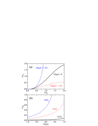
Figure 3: Quasiparticle lifetime of attractive polarons as a function of temperature at fixed coupling strengths (a) and as a function of coupling strength at given temperatures (b).

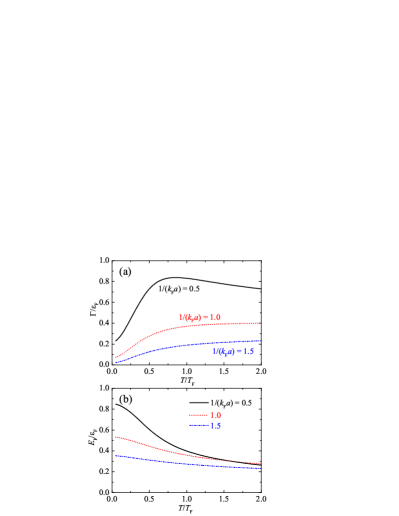
Figure 4: Quasiparticle lifetime (a) and energy (b) of repulsive polarons as a function of temperature at fixed coupling strengths: $1/(k_{F}a)=0.5$ (black solid lines), $1.0$ (red dotted lines), and $1.5$ (blue dot-dashed lines).

In Fig. 3, we show the decay rate $\Gamma$ of attractive polarons, which corresponds to the FWHM of the attractive polaron peak if it exists, as functions of temperature and interaction parameter. In general, the decay rate increases with increasing both $T$ (Fig. 3(a)) and $1/(k_{F}a)$ (Fig. 3(b)). At low temperatures, the decay rate has a $T^{2}$-dependence, according to the Fermi liquid theory FermiLiquidTheory . In the unitary limit, we find numerically that $\Gamma/\varepsilon_{F}\simeq 0.75(T/T_{F})^{2}$ for $T<T_{F}$. Above the Fermi degeneracy, there is a clear deviation from the $T^{2}$ law, indicating the breakdown of the quasiparticle description in terms of Fermi polarons.

In Fig. 4(a), we report the decay rate of repulsive polarons on the BEC side. The decay rate typically decreases with increasing interaction parameter $1/(k_{F}a)$. It also generally increases with increasing temperature. An exception occurs close to the Feshbach resonance. For $1/(k_{F}a)=0.5$, we find that there is non-monotonic dependence of the decay rate on the temperature. The decay rate attains a maximum value $\sim 0.8\varepsilon_{F}$ at about $0.8T_{F}$. Above this temperature, the decay rate starts to slowly decrease. The slow decrease is in line with the observation of a slight reduction in the spectral width of the repulsive polaron peak in Fig. 2(c) at large temperature. In Fig. 4(b), we also report the energy of repulsive polarons, which decreases monotonically with increasing temperature.

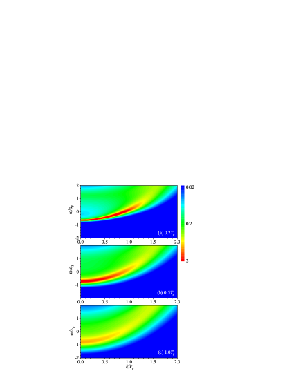
Figure 5: The two-dimensional contour plot of the finite-momentum impurity spectral function $A(\mathbf{k},\omega$) at three temperatures: $T/T_{F}=0.2$ (a), $0.5$ (b), and $1.0$ (c). Each plot is shown in the logarithmic scale. We consider the unitary coupling strength $1/(k_{F}a)=0$.

As a brief conclusion of this section, in the weak-coupling regime (i.e., the BCS side for attractive polarons and the BEC side for repulsive polarons), the polaron quasiparticle is robust against thermal fluctuations and remains well-defined above Fermi degeneracy. While in the strong-coupling regime or the unitary limit, attractive Fermi polaron exists at $T\lesssim T_{F}$. Above this characteristic temperature, we find a co-existence of the remnant of the attractive Fermi polaron and of an enhanced incoherent background. The latter might be understood as the precursor of a repulsive polaron at large temperature.

IV Ejection rf-spectroscopy in the unitary limit

In experiments, quasiparticle properties of Fermi polarons can be conveniently measured by using either ejection or injection rf-spectroscopy Schirotzek2009 ; Koschorreck2012 ; Kohstall2012 ; Scazza2017 ; Zan2019 . In most cases, the measured spectroscopy is not momentum resolved, since the density of impurities should be dilute enough, which sets a limitation on signal that brings difficulty for resolving the momentum distribution of transferred atoms. In other words, the spectroscopy is an averaged spectral function over all momenta. In Fig. 5, we show the spectral function of a unitary Fermi polaron in the $\omega$-$k$ plane at three typical temperatures. The non-trivial momentum dependence of the spectral function suggests that we may need to carefully examine the dependence of the rf-spectroscopy on the density of impurities.

In more detail, in the ejection rf-spectrosocpy scheme, a system of strongly interacting Fermi polarons is initially prepared and then a rf pulse transfers impurities to a third, unoccupied hyperfine state. In the absence of the final-state effect (i.e., the transferred impurity atom does not interact with the Fermi sea) and in the linear response regime, the transfer rate as a function of the energy $\omega$, defined as the ejection rf spectrum, is given by Mulkerin2019 ; Liu2020 ; Torma2014 ; Punk2007 ; NoteImpuritymu ,

$$I\left(\omega\right)=\sum_{\mathbf{k}}A\left[\mathbf{k},\epsilon_{\mathbf{k}}^{(I)}-\omega\right]f\left(\epsilon_{\mathbf{k}}^{(I)}-\omega-\mu_{I}\right).$$ (17)

Here, $\mu_{I}$ is the impurity chemical potential. The introduction of $\mu_{I}$ and the Fermi-Dirac distribution function is necessary to account for the finite impurity density $n_{\textrm{imp}}$ in experiments:

$$n_{\textrm{imp}}=\sum_{\mathbf{k}}\intop_{-\infty}^{\infty}d\omega A\left(\mathbf{k},\omega\right)f\left(\omega-\mu_{I}\right).$$ (18)

It is easy to see that the ejection rf spectrum is normalized to the impurity density, i.e., $\int d\omega I(\omega)=n_{\textrm{imp}}$. In the single impurity limit, $n_{\textrm{imp}}\rightarrow 0$ and $\mu_{I}\rightarrow-\infty$ at finite temperature. In this idealized case, we may replace the Fermi-Dirac distribution function by a classical Boltzmann distribution Liu2020 , $f(\omega-\mu_{I})\simeq e^{-\beta\omega}e^{\beta\mu_{I}}$. Therefore, we obtain,

$$n_{\textrm{imp}} = e^{\beta\mu_{I}}\sum_{\mathbf{k}}\intop_{-\infty}^{\infty}d\omega e^{-\beta\omega}A\left(\mathbf{k},\omega\right),$$ (19)

$$I\left(\omega\right) = e^{\beta\mu_{I}}\sum_{\mathbf{k}}e^{-\beta\epsilon_{\mathbf{k}}^{(I)}}e^{\beta\omega}A\left[\mathbf{k},\epsilon_{\mathbf{k}}^{(I)}-\omega\right].$$ (20)

By removing the unknown impurity fugacity $e^{\beta\mu_{I}}$, we arrive at an elegant expression first derived by Meera Parish and her co-workers Liu2020 ,

$$\frac{I\left(\omega\right)}{n_{\textrm{imp}}}=e^{\beta\mathcal{F}}e^{\beta\omega}\sum_{\mathbf{k}}e^{-\beta\epsilon_{\mathbf{k}}^{(I)}}A\left[\mathbf{k},\epsilon_{\mathbf{k}}^{(I)}-\omega\right],$$ (21)

where the quantity $\mathcal{F}(T)$ define by NoteFreeEnergy

$$e^{-\beta\mathcal{F}}\equiv\sum_{\mathbf{k}}\intop_{-\infty}^{\infty}d\omega e^{-\beta\omega}A\left(\mathbf{k},\omega\right)$$ (22)

can be physically interpreted as the impurity free energy. This is readily seen in the free-particle limit, where $A(\mathbf{k},\omega)=\delta(\omega-\epsilon_{\mathbf{k}}^{(I)})$ and $\mathcal{F}_{0}(T)$ given by $e^{-\beta\mathcal{F}_{0}}\equiv\sum_{\mathbf{k}}e^{-\beta\epsilon_{\mathbf{k}}^{(I)}}$ is the free energy of a free particle.

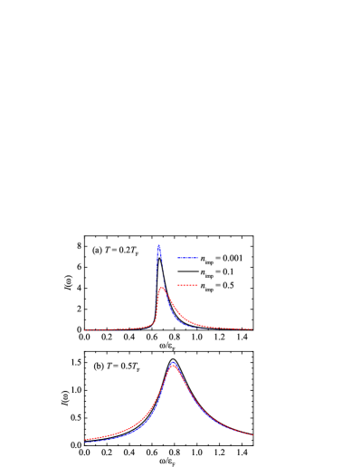
Figure 6: The ejection rf spectra of a unitary Fermi polaron at temperatures $T=0.2T_{F}$ (a) and $T=0.5T_{F}$ (b), at three impurity densities as indicated. The curves are normalized to unity, i.e., $\int d\omega I(\omega)=1$. This can be simply achieved by dividing $I(\omega)$ the impurity density $n_{\textrm{imp}}$.

Let us focus on the unitary coupling. In Fig. 6, we examine the density dependence of the ejection rf spectra of Fermi polarons in the unitary limit at two characteristic temperatures. The curves with $n_{\textrm{imp}}/n=0.001$ can be well-understood as the single-impurity limit. We find that the spectrum changes slightly if we increase the impurity density to $n_{\textrm{imp}}/n=0.1$, a typical density used in the recent MIT measurements Zan2019 . This indicates that the polaron limit is well-reached in the experiment. By further increasing impurity density to 0.5, the rf spectrum at low temperature (a, $T=0.2T_{F}$) changes appreciably: the peak position shifts to high energy and there is a significant broadening in the line shape. At large temperature (b, $T=0.5T_{F}$), however, the change is not notable. At this temperature, the effective reduced temperature for impurity is about $T/[(0.5)^{2/3}T_{F}]\simeq 0.8$, which is close to the Fermi degeneracy. Therefore, the impurity may already behave classically, following the Boltzmann distribution. This explains the weak density dependence of the rf spectrum at high temperature observed in Fig. 6(b).

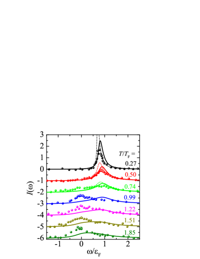
Figure 7: The comparison of the theory (lines) with the experimental data from MIT (circles) Zan2019 , for the ejection rf spectra of a unitary Fermi polaron at various temperatures (as indicated). For clarity, the origin for the theoretical curves and the experimental data at different temperatures has been down-shifted. We have applied a Lorentzian broadening on all the solid theoretical curves to take into account a well-calibrated experimental energy resolution $0.1\varepsilon_{F}$ Zan2019 , and have also right-shifted the curves by an amount $0.09\varepsilon_{F}$ to eliminate the residual final-state effect Zan2019 . At the three lowest temperatures, the theoretical curves without broadening and shift are shown by dot-dashed lines. In the comparison, we do not include any adjustable free parameters. The impurity density is taken as $n_{\textrm{imp}}=0.1$, following the experimental condition Zan2019 . The spectra are normalized to unity, $\int d\omega I(\omega)=1$.

In Fig. 7, we compare our theoretical predictions on the ejection rf spectrum with the data from the recent MIT experiment Zan2019 , without any fitting parameters. To account for a background energy resolution $0.1\varepsilon_{F}$ Zan2019 , we have taken a convolution of the theoretical curves with a Lorentzian profile. There is also a weak final-state effect due to the residual scattering length $a_{f}$ between the third hyperfine state and the fermionic atom state, as characterized by an interaction parameter $k_{F}a_{f}\simeq 0.2$ Schirotzek2009 ; Zan2019 . In equilibrium, the final state therefore is better described as a repulsive polaron state with energy $\mathcal{E}_{P}^{(f)}\simeq[4k_{F}a_{f}/(3\pi)]\varepsilon_{F}\simeq 0.09\varepsilon_{F}$ and a thermal (temperature-dependent) decay rate $\Gamma^{(f)}$ at most a few percent of Fermi energy. By neglecting $\Gamma^{(f)}$, this gives rise to a mean-field blue shift $0.09\varepsilon_{F}$ to the spectrum, which we have taken into account in the comparison.

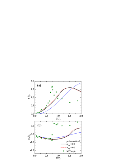
Figure 8: The FWHM width (a) and the peak position (b), extracted from the rf spectra of a unitary Fermi polaron, as a function of temperature. We compare the theoretical predictions (after spectral broadening and shift) at $n_{\textrm{imp}}=0.1$ (black solid lines) and $n_{\textrm{imp}}=0.5$ (red dotted lines), with the experimental data from MIT (circles) Zan2019 . The blue dot-dashed lines in (a) and (b) show the quasiparticle lifetime and energy of the ground-state attractive polaron at zero momentum, respectively.

We find a good agreement between theory and experiment for the spectra at positive energy (i.e., $\omega>0.5\varepsilon_{F}$), for all the temperatures considered in the comparison. As the positive energy part of the ejection rf spectrum contributed mainly by attractive polarons (or their remnant), this remarkable agreement clearly indicates that our non-self-consistent $T$-matrix theory provides a satisfactory description of ground-state attractive Fermi polarons at arbitrary temperatures. Furthermore, at low temperatures (i.e., $T\leq 0.5T_{F}$), as the spectrum is dominated by the coherent quasiparticle contribution, the agreement is good for all values of the energy.

At the temperature above $0.5T_{F}$, however, there is a growing contribution in the experimental data, centered around the zero energy $\omega\sim 0$. Roughly speaking, this contribution might be understood as the precursor of the excited branch of repulsive polarons, as we discussed earlier. Our non-self-consistent theory seems to strongly underestimate the magnitude of this excited branch. There are two potential sources for the discrepancy: the lack of either the self-energy renormalization or vertex renormalization in the theory. The former is due to the use of a bare, non-interacting impurity Green function in the vertex function (see Eq. (3)). This self-energy renormalization might be obtained by adopting a self-consistent many-body $T$-matrix theory Hu2018 . The vertex renormalization is more difficult to achieve, as we need to go beyond the ladder approximation or the $T$-matrix framework Roulet1969 .

There are also two unlikely reasons for the discrepancy. The first one is the final-state effect. Although we consider the mean-field shift due to the scattering length $a_{f}$ (that corresponds to the self-energy correction to the final state Green function), we also need to examine the so-called Aslamazov-Larkin (AL) contribution to the rf spectrum Haussmann2009 ; Pieri2009 . On the other hand, as we consider the dilute polaron limit, we completely neglect the residual repulsive interaction between polarons. Unfortunately, a quantitative treatment of either the final-state effect or the polaron-polaron interaction is difficult.

In Fig. 8, we report the comparison for the width and peak position, extracted from the experimental data Zan2019 (circles) or from our theoretically predicted ejection rf spectra (solid lines). Here, for clarity we have removed in the experimental data the background energy resolution $0.1\varepsilon_{F}$ for the width and the mean-field shift $0.09\varepsilon_{F}$ for the peak position. The width is commonly understood as the decay rate of Fermi polarons and the peak position in the ejection spectrum corresponds to the polaron energy (i.e., $-\mathcal{E}_{P}$). This common interpretation is only qualitatively useful, as the rf spectrum is not momentum-resolved. To see this, we have included in Fig. 8 the decay rate and polaron energy calculated at zero momentum (see the blue dot-dashed lines). It is clear that the width extracted from the rf spectrum differs significantly from the zero-momentum decay rate at all temperature, due to the momentum average. The peak position seems to agree with the zero-momentum polaron energy at very low temperatures. However, there is an appreciable difference once the temperature $T>0.5T_{F}$.

For the comparison between the theory and experiment for the width and peak position, we find a quantitative agreement at $T\leq 0.5T_{F}$, consistent with the observation in Fig. 7. Above this temperature, the experimental width increases sharply and peaks at about $0.75T_{F}$, at which the peak position suddenly jumps to zero energy. All these features are related to the enhanced excited branch of repulsive polarons, which unfortunately can not be account for by our non-self-consistent many-body $T$-matirx theory, as we emphasized earlier.

It is worth noting that the theoretical width and peak position have previously been calculated within similar non-self-consistent $T$-matrix theory at finite impurity density Mulkerin2019 ; Tajima2019 . An attempt Tajima2019 was also made to understand the MIT data in Fig. 8. Our results focus on the physical limit of a single impurity, with the uncertainty from numerical analytic continuation removed. Moreover, our new comparison for the ejection rf spectra in Fig. 7 clearly reveals the key reason for the discrepancy. That is, we need to find a more adequate theoretical description for the excited branch of repulsive polarons at high temperature.

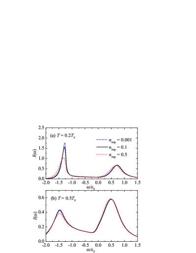
Figure 9: The injection rf spectra of a Fermi polaron at temperatures $T=0.2T_{F}$ (a) and $T=0.5T_{F}$ (b), at three impurity densities as indicated. Here, we take the coupling strength $1/(k_{F}a)=0.5$. The curves are normalized to the unity, $\int d\omega I(\omega)=1$.

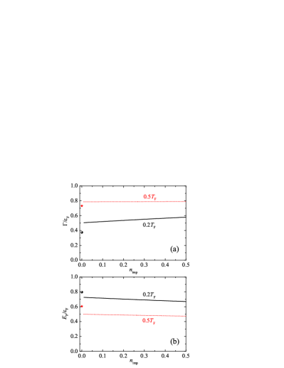
Figure 10: The width (a) and the peak position (b), extracted from the injection rf spectra at $1/(k_{F}a)=0.5$, as a function of the impurity density $n_{\textrm{imp}}$ at temperatures $T=0.2T_{F}$ (black solid lines) and $T=0.5T_{F}$ (red dotted lines). The symbols at zero impurity density show the quasiparticle lifetime or the energy of the zero-momentum repulsive polaron.

V Injection rf-spectroscopy of repulsive polarons

Let us now turn to a reversed scheme of the injection rf-spectroscopy, where the impurities initially occupy the non-interacting (or weakly-interacting) third hyperfine state and are then transferred to the strongly-interacting polaron state. This scheme is useful to probe the excited repulsive polaron branch Scazza2017 , which can hardly be detected in the standard ejection rf spectroscopy due to its negligible thermal occupation. By neglecting the initial-state effect, the injection rf spectrum is given by Mulkerin2019 ; Liu2020 ; Torma2014 ,

$$I\left(\omega\right)=\sum_{\mathbf{k}}A\left[\mathbf{k},\epsilon_{\mathbf{k}}^{(I)}+\omega\right]f\left(\epsilon_{\mathbf{k}}^{(I)}-\mu_{i}\right),$$ (23)

where $\mu_{i}$ is the impurity chemical potential in the initial third hyperfine state, to be determined by the number equation, $n_{\textrm{imp}}=\sum_{\mathbf{k}}f(\epsilon_{\mathbf{k}}^{(I)}-\mu_{i})$. In the idealized single-impurity limit ($\mu_{i}\rightarrow-\infty$ at nonzero temperature), once again we can write $n_{\textrm{imp}}=e^{\beta\mu_{i}}\sum_{\mathbf{k}}e^{-\beta\epsilon_{\mathbf{k}}^{(I)}}$ and

$$\frac{I\left(\omega\right)}{n_{\textrm{imp}}}=e^{\beta\mathcal{F}_{0}}\sum_{\mathbf{k}}e^{-\beta\epsilon_{\mathbf{k}}^{(I)}}A\left[\mathbf{k},\epsilon_{\mathbf{k}}^{(I)}+\omega\right].$$ (24)

A comparison with Eq. (21) gives us a very simple relation between the ejection and injection rf spectra in the single-impurity Boltzmann limit Liu2020 ,

$$I_{\textrm{ej}}\left(\omega\right)=e^{\beta\Delta\mathcal{F}}e^{\beta\omega}I_{\textrm{inj}}\left(-\omega\right),$$ (25)

where $\Delta\mathcal{F}(T)\equiv\mathcal{F}-\mathcal{F}_{0}$ and the subscripts “ej” and “inj” indicate the ejection and injection spectra, respectively.

In Fig. 9, we show the injection rf spectra at the interaction parameter $1/(k_{F}a)=0.5$ and at various impurity densities. Two peaks are clearly visible at negative and positive energies, contributed from the attractive and repulsive polarons, respectively. For the attractive polaron peak, its density dependence is similar to what we have seen in Fig. 6. For the repulsive polaron peak, the density dependence turns out to be very weak.

In Fig. 10, we examine in a more careful way the weak density dependence of the width and peak position of repulsive polarons. We are specifically interested in comparing the width and peak position in the dilute limit with the decay rate and polaron energy at zero momentum, which are indicated in the figure by symbols. It is readily seen that, due to the momentum average in the injection rf spectrum, in the single-impurity limit the width differs from the zero-momentum decay rate and the peak position does not locate at the polaron energy.

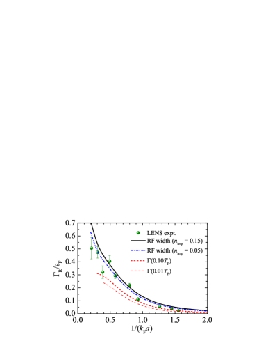
Figure 11: The width of the repulsive polaron extracted from the injection rf spectrum as a function of coupling constant $1/(k_{F}a)$ at two impurity densities $n_{\textrm{imp}}=0.15$ (black solid line) and $n_{\textrm{imp}}=0.05$ (blue dot-dashed line). The temperature is set to be $T=0.1T_{F}$. We compare our theoretical predictions to the experimental data measured from coherent Rabi oscillations at $T=0.10(2)T_{F}$ and $n_{\textrm{imp}}=0.15(1)$ Scazza2017 . We show also the decay rate of the zero-momentum repulsive polaron at the temperatures $T=0.1T_{F}$ (thick red dashed line) and $T=0.01T_{F}$ (thin red dashed line).

This difference may provide a natural explanation for the discrepancy between theory and experiment for the quasiparticle lifetime of repulsive polarons, as recently measured at LENS by using coherent Rabi oscillations Scazza2017 . This is shown in Fig. 11, where the data (green circles with error bar) are compared with the predictions from Chevy’s ansatz at essentially zero temperature (thin red dashed line at $0.01T_{F}$) and at the experimental temperature (thick red dashed line at $0.10T_{F}$). At the interaction parameter $1/(k_{F}a)<1$, the measured decay rate is significantly larger than the theoretical prediction. In a recent theoretical simulation Adlong2020 , a finite-temperature variational approach has been used to simulate the real-time dynamics of Rabi oscillations. However, the simulation is carried out at zero momentum and hence yields a similar prediction from the finite-temperature Chevy’s ansatz (see, i.e., the thick red dashed line at $0.10T_{F}$).

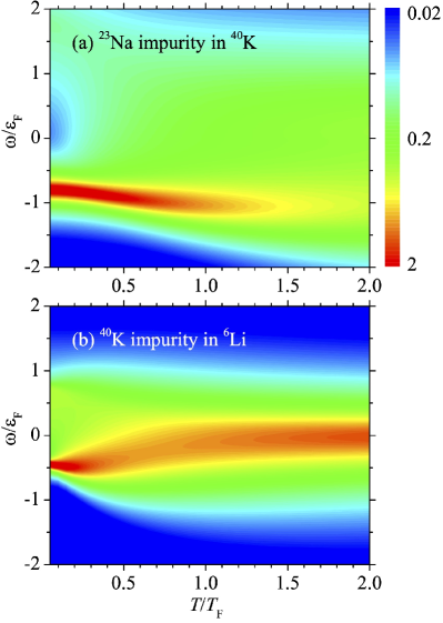
Figure 12: The two-dimensional contour plot of the temperature evolution of the zero-momentum impurity spectral function $A(\mathbf{k}=0,\omega$) for two kinds of Fermi polarons with a unitary coupling strength $1/(k_{F}a)=0$: ²³Na impurity in a Fermi sea of ⁴⁰K atoms (a) and ⁴⁰K impurity in a Fermi sea of ⁶Li atoms (b). Each plot is shown in the logarithmic scale.

Physically, the impurity can have a thermal distribution over different momenta during a coherent Rabi oscillation, so we need to consider the momentum average. Therefore, it is reasonable to assume that the measured decay rate from Rabi oscillations might be identical to the width measured from the injection rf spectrum. In Fig. 11, we plot the width of repulsive polarons extracted from the theoretical injection rf spectra, which are calculated at $T=0.1T_{F}$ and at either the averaged experimental impurity density $n_{\textrm{imp}}\simeq 0.15$ (black solid line) Scazza2017 or the minimum experimental impurity density $n_{\textrm{imp}}\simeq 0.05$ (blue dot-dashed line) Scazza2017 . As anticipated, we find a much improved agreement between theory and experiment, confirming the importance of the inclusion of the momentum average.

VI Quasiparticle lifetime at unequal mass

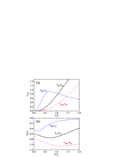
Figure 13: Quasiparticle lifetime (a) and energy of unitary Fermi polarons as a function of temperature. Here, we consider three experimental setups: ²³Na impurity in a Fermi sea of ⁴⁰K atoms (red dotted lines), ⁶Li impurity in a Fermi sea of ⁶Li atoms (solid lines), and ⁴⁰K impurity in a Fermi sea of ⁶Li atoms (blue dot-dashed lines).

We finally consider the situation that the impurity and fermionic atoms have different masses. These cases can easily realized in experiments by using heteronuclear atomic mixtures, such as ²³Na-⁴⁰K and ⁴⁰K-⁶Li mixtures. Let us focus on the most interesting strongly-interacting limit with unitary coupling $1/(k_{F}a)=0$.

In Fig. 12, we present the time-evolution of the zero-momentum impurity spectral function in the form of contour plots, for a light impurity in heavy medium (a, ²³Na in a Fermi sea of ⁴⁰K atoms with $\alpha\simeq-0.27$) or a heavy impurity in light medium (b, ⁴⁰K in a Fermi sea of ⁶Li atoms with $\alpha\simeq 0.74$). For the former, there is no qualitative change, in comparison with the equal mass case as reported in Fig. 1(b). In contrast, for the heavy impurity case, we observe a dramatic change. As can be seen from Fig. 12(b), by increasing temperature the polaron peak quickly moves to zero energy. The width of the peak initially increases with temperature. At around the Fermi temperature, however, the width starts to become narrower. At the largest temperature considered in the figure $T=2T_{F}$, the width reduces to about $0.5\varepsilon_{F}$. This temperature evolution of the width can be seen more clearly in Fig. 13(a), where we plot the decay rate as a function of temperature.

It is interesting to note that, this non-monotonic temperature dependence of the decay rate has been previously seen in repulsive polarons close to the Feshbach resonance, see, for example, the curve in Fig. 4(a) for $1/(k_{F}a)=0.5$. Therefore, it seems reasonable to assume that for a sufficiently heavy impurity with unitary coupling, the attractive polaron may smoothly turn into (or more precisely, acquire the characteristic of) a repulsive polaron at large temperature. It is also worth noting that the temperature dependence of the decay rate and the polaron energy of the ⁴⁰K/⁶Li case is qualitatively similar to what we have observed in the experimental data for the width and peak position of the rf spectroscopy Zan2019 , as reported in Fig. 8, although the latter is for the equal mass case (i.e., ⁶Li/⁶Li) and there is a momentum-average in the ejection rf spectrum, as we frequently emphasized.

VII Conclusions and outlooks

In summary, we have presented a systematic study of finite-temperature quasiparticle properties of Fermi polarons, by using the well-established non-self-consistent many-body $T$-matrix theory Combescot2007 . Different from the previous works Mulkerin2019 ; Tajima2019 , we have focus on the single-impurity limit, and have accurately calculated the impurity spectral function and the associated ejection and injection radio-frequency (rf) spectroscopies, by avoiding the ill-defined numerical analytic continuation. Our non-self-consistent $T$-matrix calculations also complement the earlier theoretical investigations based on a finite-temperature variational approach Liu2019 ; Liu2020 .

One key result of this work is that we have clarified the important role played by the momentum-average, which is unavoidable in the current rf spectroscopy. As a result, the experimentally measured peak position and width from the rf spectroscopy do not exactly correspond to the polaron energy and decay rate. In particular, the measured width can differ significantly from the decay rate of Fermi polarons at zero momentum that we want to determine. By taking into account the crucial role of momentum-average, we have successfully explained the measured ejection rf spectrum of a unitary Fermi polaron at low temperatures (i.e., $T<0.5T_{F}$) from the MIT group Zan2019 . We have also resolved a puzzling discrepancy between theory and experiment for the quasiparticle lifetime of repulsive polarons, observed in a recent experiment at LENS Scazza2017 ; Adlong2020 .

The non-self-consistent $T$-matrix theory seems to work very well for weak-coupling Fermi polarons (i.e., attractive polarons on the BCS side and repulsive polarons on the BEC side). In the strong-coupling unitary limit, the comparison between the theory and the MIT experiment indicates that the theory also provides a satisfactory description of attractive Fermi polarons at arbitrary temperatures. However, the theory seems to strongly underestimates the precursor of repulsive polarons near and above the Fermi degenerate temperature. We believe this is due to the inadequate description of the vertex function, which plays the role of the molecule Green function. In future studies for an improved theory, it will be useful to consider the self-energy renormalization and vertex renormalization Roulet1969 .

Appendix A The many-body part of the two-particle propagator $\chi_{R}^{(mb)}$

In Eq. (15), let us introduce a new variable $\mathbf{p}=\mathbf{k}+(1-\alpha)\mathbf{q}/2$, and rewrite the expression into the form,

$$\chi_{R}^{(mb)}=\frac{1+\alpha}{4\pi^{2}}\intop_{0}^{\infty}\frac{dpg\left(p\right)p^{2}}{\frac{1+\alpha}{2}\left[\Omega^{+}+\mu-\frac{\left(1-\alpha\right)}{2}q^{2}\right]-p^{2}},$$ (26)

where we have defined an angle-integrated function ($z=e^{\beta\mu}$ is the fugacity),

$$g\left(p\right) \equiv\intop_{-1}^{+1}\frac{dx}{2}f\left[p^{2}+\frac{\left(1-\alpha\right)^{2}}{4}q^{2}+\left(1-\alpha\right)pqx-\mu\right]$$

$$=\frac{1}{2\left(1-\alpha\right)\beta pq}\ln\left(\frac{1+ze^{-\beta\left[p-\frac{1-\alpha}{2}q\right]^{2}}}{1+ze^{-\beta\left[p+\frac{1-\alpha}{2}q\right]^{2}}}\right).$$ (27)

The integral Eq. (26) is well defined if

$$-x^{2}\equiv\frac{1+\alpha}{2}\left[\Omega+\mu-\frac{\left(1-\alpha\right)}{2}q^{2}\right]<0.$$

In this case, we find that,

$$\textrm{Re}\chi_{R}^{(mb)} = -\frac{1+\alpha}{4\pi^{2}}\intop_{0}^{\infty}dp\frac{p^{2}}{p^{2}+x^{2}}g\left(p\right),$$ (28)

$$\textrm{Im}\chi_{R}^{(mb)} = 0.$$ (29)

Otherwise, let us define

$$y\equiv\frac{1+\alpha}{2}\left[\Omega+\mu-\frac{\left(1-\alpha\right)}{2}q^{2}\right]\geq 0$$

and use the identity (the notation P.V. means taking Cauchy principle value)

$$\frac{1}{X+i0^{+}}=\mathcal{\textrm{P.V.}}\left(\frac{1}{X}\right)-i\pi\delta\left(X\right)$$ (30)

to rewrite the real and imaginary parts of $\chi_{R}^{(mb)}$:

$$\textrm{Re}\chi_{R}^{(mb)} =-\frac{1+\alpha}{4\pi^{2}}\textrm{P.V.}\intop_{0}^{\infty}dp\frac{p^{2}g\left(p\right)}{p^{2}-y}$$

$$=-\frac{1+\alpha}{8\pi^{2}}\left(C_{1}+C_{2}\right)$$ (31)

and

$$\textrm{Im}\chi_{R}^{(mb)} =\frac{1+\alpha}{4\pi^{2}}\left(-\pi\right)\intop_{0}^{\infty}dpg\left(p\right)p^{2}\delta\left(y-p^{2}\right)$$

$$=-\frac{1+\alpha}{8\pi}\sqrt{y}g\left(\sqrt{y}\right).$$ (32)

Here, by taking Cauchy principle value we have defined two integrals,

$$C_{1} \equiv \intop_{y}^{\infty}\frac{d\xi}{\xi}\sqrt{y+\xi}g\left(\sqrt{y+\xi}\right),$$

$$C_{2} \equiv \intop_{0}^{y}d\xi\frac{\sqrt{y+\xi}g\left(\sqrt{y+\xi}\right)-\sqrt{y-\xi}g\left(\sqrt{y-\xi}\right)}{\xi}.$$

The numerical calculation of $\textrm{Re}\chi_{R}^{(mb)}$ and $\textrm{Im}\chi_{R}^{(mb)}$ therefore involves only the one-dimensional integral, which is very efficient to carry out.

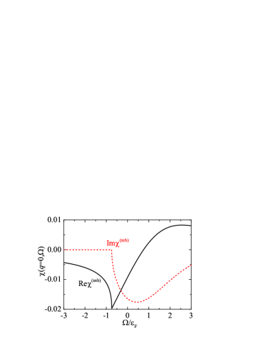
Figure 14: The real and imaginary parts of $\chi_{R}^{(mb)}(\mathbf{q}=0,\Omega)$, in arbitrary units, at the temperature $T=0.5T_{F}$.

In Fig. 14, we show $\chi_{R}^{(mb)}(\mathbf{q}=0,\Omega)$ at a typical temperature $T=0.5T_{F}$. The imaginary part becomes nonzero once the frequency is above the threshold $\Omega_{c}(\mathbf{q})=(1-\alpha)q^{2}/2-\mu$, where the chemical potential $\mu(T)$ is the temperature dependent. As a result, there is a sharp kink in the real part $\textrm{Re}\chi_{R}^{(mb)}$.

In general, $\textrm{Re}\chi_{R}<0$ for $\Omega<\Omega_{c}(\mathbf{q})$. However, with $1/(k_{F}a)>0$ we may have $\textrm{Re}\chi_{R}=0$ at a certain value $\Omega<\Omega_{c}(\mathbf{q})$ and hence a pole in the two-particle vertex function. This indicates the formation of an undamped molecule excitation below the two-particle threshold.

References

- (1) A. S. Alexandrov and J. T. Devreese, Advances in Polaron Physics (Springer, New York, 2010), Vol. 159.
- (2) L. D. Landau, Electron Motion in Crystal Lattices, Phys. Z. Sowjetunion 3, 664 (1933).
- (3) G. D. Mahan, Excitons in Metals: Infinite Hole Mass, Phys. Rev. 163, 612 (1967).
- (4) B. Roulet, J. Gavoret, and P. Nozières, Singularities in the X-Ray Absorption and Emission of Metals. I. First-Order Parquet Calculation, Phys. Rev. 178, 1072 (1969).
- (5) P. Nozières and C. T. De Dominicis, Singularities in the X-Ray Absorption and Emission of Metals. III. One- Body Theory Exact Solution, Phys. Rev. 178, 1097 (1969).
- (6) J. Bardeen, G. Baym, and D. Pines, Effective Interaction of He3 Atoms in Dilute Solutions of He3 in He4 at Low Temperatures, Phys. Rev. 156, 207 (1967).
- (7) P. Massignan, M. Zaccanti, and G. M. Bruun, Polarons, dressed molecules and itinerant ferromagnetism in ultracold Fermi gases, Rep. Prog. Phys. 77, 034401 (2014).
- (8) Z. Lan and C. Lobo, A single impurity in an ideal atomic Fermi gas: current understanding and some open problems, J. Indian Inst. Sci. 94, 179 (2014).
- (9) R. Schmidt, M. Knap, D. A. Ivanov, J.-S. You, M. Cetina, and E. Demler, Universal many-body response of heavy impurities coupled to a Fermi sea: a review of recent progress, Rep. Prog. Phys. 81, 024401 (2018).
- (10) I. Bloch, J. Dalibard, and W. Zwerger, Many-body physics with ultracold gases, Rev. Mod. Phys. 80, 885 (2008).
- (11) C. Chin, R. Grimm, P. Julienne, and E. Tiesinga, Feshbach resonances in ultracold gases, Rev. Mod. Phys. 82, 1225 (2010).
- (12) A. Schirotzek, C.-H. Wu, A. Sommer, and M.W. Zwierlein, Observation of Fermi Polarons in a Tunable Fermi Liquid of Ultracold Atoms, Phys. Rev. Lett. 102, 230402 (2009).
- (13) Y. Zhang, W. Ong, I. Arakelyan, and J. E. Thomas, Polaron-to-Polaron Transitions in the Radio-Frequency Spectrum of a Quasi-Two-Dimensional Fermi Gas, Phys. Rev. Lett. 108, 235302 (2012).
- (14) C. Kohstall, M. Zaccanti, M. Jag, A. Trenkwalder, P. Massignan, G.M. Bruun, F. Schreck, and R. Grimm, Metastability and coherence of repulsive polarons in a strongly interacting Fermi mixture, Nature (London) 485, 615 (2012).
- (15) M. Koschorreck, D. Pertot, E. Vogt, B. Fröhlich, M. Feld, and M. Köhl, Attractive and repulsive Fermi polarons in two dimensions, Nature (London) 485, 619 (2012).
- (16) M. Cetina, M. Jag, R. S. Lous, I. Fritsche, J. T. M.Walraven, R. Grimm, J. Levinsen, M. M. Parish, R. Schmidt, M. Knap, and E. Demler, Ultrafast many-body interferometry of impurities coupled to a Fermi sea, Science 354, 96 (2016).
- (17) M.-G. Hu, M. J. Van de Graaff, D. Kedar, J. P. Corson, E. A. Cornell, and D. S. Jin, Bose Polarons in the Strongly Interacting Regime, Phys. Rev. Lett. 117, 055301 (2016).
- (18) N. B. Jørgensen, L. Wacker, K. T. Skalmstang, M. M. Parish, J. Levinsen, R. S. Christensen, G. M. Bruun, and J. J. Arlt, Observation of Attractive and Repulsive Polarons in a Bose-Einstein Condensate, Phys. Rev. Lett. 117, 055302 (2016).
- (19) F. Scazza, G. Valtolina, P. Massignan, A. Recati, A. Amico, A. Burchianti, C. Fort, M. Inguscio, M. Zaccanti, and G. Roati, Repulsive Fermi Polarons in a Resonant Mixture of Ultracold 6Li Atoms, Phys. Rev. Lett. 118, 083602 (2017).
- (20) Z. Yan, P. B. Patel, B. Mukherjee, R. J. Fletcher, J. Struck, and M.W. Zwierlein, Boiling a Unitary Fermi Liquid, Phys. Rev. Lett. 122, 093401 (2019).
- (21) Z. Z. Yan, Y. Ni, C. Robens, and M.W. Zwierlein, Bose polarons near quantum criticality, Science 368, 190 (2020).
- (22) G. Ness, C. Shkedrov, Y. Florshaim, O. K. Diessel, J. von Milczewski, R. Schmidt, and Y. Sagi, Observation of a Smooth Polaron-Molecule Transition in a Degenerate Fermi Gas, Phys. Rev. X 10, 041019 (2020).
- (23) F. Chevy, Universal phase diagram of a strongly interacting Fermi gas with unbalanced spin populations, Phys. Rev. A 74, 063628 (2006).
- (24) R. Combescot, A. Recati, C. Lobo, and F. Chevy, Normal State of Highly Polarized Fermi Gases: Simple Many-Body Approaches, Phys. Rev. Lett. 98, 180402 (2007).
- (25) N. Prokof’ev and B. Svistunov, Fermi-polaron problem: Diagrammatic Monte Carlo method for divergent sign-alternating series, Phys. Rev. B 77, 020408(R) (2008).
- (26) M. Punk, P. T. Dumitrescu, and W. Zwerger, Polaron-to-molecule transition in a strongly imbalanced Fermi gas, Phys. Rev. A 80, 053605 (2009).
- (27) X. Cui and H. Zhai, Stability of a fully magnetized ferromagnetic state in repulsively interacting ultracold Fermi gases, Phys. Rev. A 81, 041602(R) (2010).
- (28) P. Massignan and G. M. Bruun, Repulsive polarons and itinerant ferromagnetism in strongly polarized Fermi gases, Eur. Phys. J. D 65, 83 (2011).
- (29) R. Schmidt, T. Enss, V. Pietilä, and E. Demler, Fermi polarons in two dimensions, Phys. Rev. A 85, 021602(R) (2012).
- (30) M. M. Parish and J. Levinsen, Highly polarized Fermi gases in two dimensions, Phys. Rev. A 87, 033616 (2013).
- (31) J. Vlietinck, J. Ryckebusch, and K. Van Houcke, Quasiparticle properties of an impurity in a Fermi gas, Phys. Rev. B 87, 115133 (2013).
- (32) S. P. Rath and R. Schmidt, Field-theoretical study of the Bose polaron, Phys. Rev. A 88, 053632 (2013).
- (33) L. A. Peña Ardila and S. Giorgini , Impurity in a Bose-Einstein condensate: Study of the attractive and repulsive branch using quantum Monte Carlo methods, Phys. Rev. A 92, 033612 (2015).
- (34) J. Levinsen, M. M. Parish, and G. M. Bruun, Impurity in a Bose-Einstein Condensate and the Efimov Effect, Phys. Rev. Lett. 115, 125302 (2015).
- (35) O. Goulko, A. S. Mishchenko, N. Prokof’ev, B. Svistunov, Dark continuum in the spectral function of the resonant Fermi polaron, Phys. Rev. A 94, 051605(R) (2016).
- (36) H. Hu, B. C. Mulkerin, J. Wang, and X.-J. Liu, Attractive Fermi polarons at nonzero temperatures with a finite impurity concentration, Phys. Rev. A 98, 013626 (2018).
- (37) H. Tajima and S. Uchino, Many Fermi polarons at nonzero temperature, New J. Phys. 20, 073048 (2018).
- (38) B. C. Mulkerin, X.-J. Liu, and H. Hu, Breakdown of the Fermi polaron description near Fermi degeneracy at unitarity, Ann. Phys. (NY) 407, 29 (2019).
- (39) H. Tajima and S. Uchino, Thermal crossover, transition, and coexistence in Fermi polaronic spectroscopies, Phys. Rev. A 99, 063606 (2019).
- (40) L. A. Peña Ardila, N. B. Jørgensen, T. Pohl, S. Giorgini, G. M. Bruun, and J. J. Arlt, Analyzing a Bose polaron across resonant interactions, Phys. Rev. A 99, 063607 (2019).
- (41) W. E. Liu, J. Levinsen, and M. M. Parish, Variational Approach for Impurity Dynamics at Finite Temperature, Phys. Rev. Lett. 122, 205301 (2019).
- (42) J. Wang, X.-J. Liu, and H. Hu, Roton-Induced Bose Polaron in the Presence of Synthetic Spin-Orbit Coupling, Phys. Rev. Lett. 123, 213401 (2019).
- (43) W. E. Liu, Z.-Y. Shi, M. M. Parish and J. Levinsen, Theory of radio-frequency spectroscopy of impurities in quantum gases, Phys. Rev. A 102, 023304 (2020).
- (44) H. S. Adlong, W. E. Liu, F. Scazza, M. Zaccanti, N. D. Oppong, S. Fölling, M. M. Parish, and J. Levinsen, Quasiparticle Lifetime of the Repulsive Fermi Polaron, Phys. Rev. Lett. 125, 133401 (2020).
- (45) M. M. Parish, H. S. Adlong, W. E. Liu, and J. Levinsen, Thermodynamic signatures of the polaron-molecule transition in a Fermi gas, Phys. Rev. A 103, 023312 (2021).
- (46) R. Pessoa, S. A. Vitiello, and L. A. Peña Ardila, Finite-range effects in the unitary Fermi polaron, Phys. Rev. A 104, 043313 (2021).
- (47) H. Hu, J. Wang, J. Zhou, and X.-J. Liu, Crossover polarons in a strongly interacting Fermi superfluid, arXiv:2111.01372 (2021).
- (48) R. Haussmann, M. Punk, and W. Zwerger, Spectral functions and rf response of ultracold fermionic atoms, Phys. Rev. A 80, 063612 (2009).
- (49) D. Pines and P. Nozières, The Theory of Quantum Liquids: Vol. 1, Normal Fermi Liquids (W. A. Benjamin, New York 1966).
- (50) P. Törmä, Spectroscopies—Theory, in Quantum Gas Experiments (World Scientific, Singapore, 2014). Chap. 10, pp. 199–250.
- (51) M. Punk and W. Zwerger, Theory of rf-Spectroscopy of Strongly Interacting Fermions, Phys. Rev. Lett. 99, 170404 (2007).
- (52) We note that, in the spectral function ) the energy is measured with respect to the impurity chemical potential . This is convenient in the single impurity limit, where it is meaningless to specify .
- (53) However, this interesting expression should be used with specific care to the asymptotic behavior of the spectral function ) at large momentum and at large energy , which in general exhibits a power-law tail characterized by Tan’s contact parameter Punk2007 . As a result, the integral may diverge.
- (54) P. Pieri, A. Perali, and G. C. Strinati, Enhanced paraconductivity-like fluctuations in the radiofrequency spectra of ultracold Fermi atoms, Nature Phys. 5, 736 (2009).