Adaptive Bézier Degree Reduction and Splitting
for Computationally Efficient Motion Planning

Abstract

As a parametric polynomial curve family, Bézier curves are widely used in safe and smooth motion design of intelligent robotic systems from flying drones to autonomous vehicles to robotic manipulators. In such motion planning settings, the critical features of high-order Bézier curves such as curve length, distance-to-collision, maximum curvature/velocity/acceleration are either numerically computed at a high computational cost or inexactly approximated by discrete samples. To address these issues, in this paper we present a novel computationally efficient approach for adaptive approximation of high-order Bézier curves by multiple low-order Bézier segments at any desired level of accuracy that is specified in terms of a Bézier metric. Accordingly, we introduce a new Bézier degree reduction method, called parameterwise matching reduction, that approximates Bézier curves more accurately compared to the standard least squares and Taylor reduction methods. We also propose a new Bézier metric, called the maximum control-point distance, that can be computed analytically, has a strong equivalence relation with other existing Bézier metrics, and defines a geometric relative bound between Bézier curves. We provide extensive numerical evidence to demonstrate the effectiveness of our proposed Bézier approximation approach. As a rule of thumb, based on the degree-one matching reduction error, we conclude that an $n^{\text{th}}$-order Bézier curve can be accurately approximated by $3(n-1)$ quadratic and $6(n-1)$ linear Bézier segments, which is fundamental for Bézier discretization.

I Introduction

Safe and smooth motion planning is essential for many autonomous robots. As a parametric smooth motion representation, polynomial curves find significant applications in safe robot motion design from flying drones [1, 2, 3, 4, 5] to autonomous vehicles [6, 7, 8, 9] to robotic manipulators [10, 11, 12, 13]. Polynomials expressed in different (e.g., monomial, Taylor, and Bernstein) bases offer different useful functional and geometric properties for computationally efficient motion planning. While the monomial (a.k.a. power) basis yields quadratic trajectory optimization objectives [1], polynomial Bézier curves in Bernstein basis have useful convexity and interpolation properties [4]: a Bézier curve is contained in the convex hull of its control points (i.e., parameters), and it smoothly interpolates between the first and last control point. A well known challenge of motion planning with polynomial and so Bézier curves is that the computational complexity increases with increasing curve degree [6]. Because critical curve features such as curve length, distance-to-collision, and maximum curvature/velocity/acceleration can be analytically determined only for low-order (e.g., linear and quadratic) polynomial curves and are numerically computed or inexactly approximated using discrete samples for higher-order polynomials, as summarized in Table I.

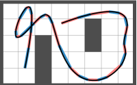
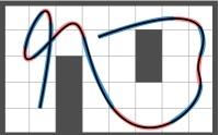
Figure 1: Adaptive approximation of an $8^{\text{th}}$-order Bézier curve (black line) by multiple (left) linear and (right) quadratic Bézier segments (red and blue patches) whose length, maximum velocity/acceleration/curvature, and distance to obstacles (dark gray) can be computed analytically. The Bézier degree reduction and splitting is automatically performed by uniform matching reduction and binary search for a maximum control-point distance of $0.1$ units.

TABLE I: Computation of Bezier Curve Features in Motion Planning

Bezier Curve Feature	$n\leq 2$	$n=3$	$n>3$
Arc Length	Analytic	Numeric	Numeric
Maximum Velocity	Analytic	Analytic	Numeric
Maximum Curvature	Analytic	Numeric	Numeric
Distance-to-Point	Analytic	Numeric	Numeric
Distance-to-Line-Segment	Analytic	Numeric	Numeric

In this paper, we propose a new computationally efficient approach for adaptive approximation of high-order Bézier curves by multiple low-order Bézier segments at any desired level of accuracy specified in terms of a Bézier metric, as illustrated in Fig. 5. Our approach is based on an unexplored functional property of Bézier curves in motion planning: distance between Bézier curves can be measured analytically in terms of control points. Accordingly, we introduce a new analytic Bézier metric, called the maximum control-point distance, that can be used to geometrically bound Bézier curves with respect to each other, and defines tight upper bounds on other existing Bézier metrics. We also propose a new Bézier degree reduction method, called parameterwise matching reduction, that allows preserving certain curve points (e.g., end points) while performing degree reduction. Based on the degree-one parameterwise matching reduction error, we conclude that an $n^{\text{th}}$-order Bézier curve can be accurately approximated by $3(n-1)$ quadratic and $6(n-1)$ linear Bézier segments, which is a fundamental rule of thumb for Bézier discretization. In numerical simulations, we demonstrate the effectiveness of approximating high-order Bézier curves by linear and quadratic Bézier segments for fast and accurate computation of common curve features used in motion planning.

I-A Motivation and Related Literature

Autonomous robots and people interacting with them enjoy smooth motion in practice: jerky robot motion does not only cause mechanical and electrical failures and malfunctions, but also causes discomfort for the user. Most existing smooth motion planning methods follow a two-step approach: first find a piecewise linear path for a simplified version of the system to achieve a simplified version of a given task; and then perform path smoothing as post-processing to satisfy the actual task and system requirements [14]. The first step, piecewise linear motion planning, is well established with many computationally effective (search- and sampling-based) planning algorithms for the fully actuated kinematic robot model [15]. The second step, path smoothing that aims to convert a piecewise linear reference plan into a smooth dynamically feasible trajectory satisfying both system and task constraints, is an active research topic, especially for real-time operation requirements. Due to their compact parametric form and functional properties, polynomial curves have recently received significant attention with promising potentials for computationally efficient path smoothing, especially for differential flat systems [16] such as cars [7, 8], quadrotors [1, 2, 3], and fixed-wing aircrafts [17], to name a few, whose control inputs can be expressed as a function of flat system outputs (represented by polynomials) and their derivatives. For example, while polynomials of degree 3-5 are often used for autonomous vehicles, polynomials of degree 5-10 are required for quadrotors. The major reason for the use of relatively low-order polynomials in practice is that the computational cost of planning with polynomials increases with increasing degree of polynomials [14, 6]. Our proposed approach enables handling high-order polynomials efficiently by approximating them with multiple low-order polynomial segments.

Convex optimization plays a key role in polynomial path smoothing. In polynomial trajectory optimization, the standard optimization objectives of total squared velocity, acceleration, jerk, and snap (i.e., the first, second, third and fourth time derivatives of the position) of a robotic system can be written as a quadratic objective function of polynomial parameters [1, 17]. In order to take the full advantage of quadratic programming, the system and task constraints are often represented as linear or quadratic inequalities. For example, a piecewise linear reference plan can be used to construct a convex safe corridor around the reference plan to represent planning constraints as a collection of convex polytopes [18] or spheres [3]. Accordingly, polynomial trajectory optimization is often formulated as a quadratic optimization problem, for example, by simply using a polynomial discretization [1, 2, 13]. This naturally raises a question about polynomial discretization: how many sample points along a polynomial are needed for a proper and accurate representation of planning constraints. The existing methods use either manual or heuristic approaches to add extra samples if polynomial discretization fails [1, 2]. In this sense, our results offer a systematic solution for determining a proper discretization of polynomials to model planning constraints at any desired level of accuracy.

In polynomial trajectory optimization, the convexity property of Bézier curves makes them an attractive choice for handling convex system constraints within quadratic programming. Since Bézier curves are contained in the convex hull of their control points, trajectory optimization constraints are often enforced by constraining Bézier control points inside convex constraint sets [4, 19, 20]. This approach is effectively applied for smooth trajectory generation with Bezier curves over safe corridors [18] in various application settings; for example, for drone navigation in unknown environments [4, 5], autonomous driving [7, 21, 20], multirobot coordination [19, 22], and perception-aware navigation [23]. Although it performs reasonably well for low-order Bézier curves in practice, this simple but conservative approach is suboptimal for high-order Bézier curves since the convex hull of Bézier control points significantly overestimates the smallest convex region containing by the actual curve, especially for higher-order polynomials. On the other hand, exact and fast continuous constraint verification with polynomial curves is possible based on the separation of polynomial extremes [24], the sign change of polynomials [25], and their root existence test based on Sturm’s theorem [26], but these methods result in highly complex nonlinear optimization constraints. Our approach for approximating high-order Bézier curves by low-order Bézier segments allows one to use the convexity of low-order Bézier curves in high-order polynomial trajectory optimization in a less conservative way.

Another appealing feature of Bézier curves for smooth robot motion design is that they smoothly interpolate between the first and last control points. This interpolation property is often leveraged for motion planning of nonholonomic systems with boundary conditions; for example, for waypoint smoothing [27, 28, 9] and smooth steering control [29, 30] in autonomous driving [31, 32], and path smoothing in sampling-based motion planning [33, 34, 35, 11]. Continuous curvature path smoothing with curvature constraints is applied for increasing passenger comfort while ensuring dynamical feasibility in autonomous vehicles for smooth lane change [36] and urban driving [8, 37, 38, 39]. Although path smoothing with curvature constraints can be performed analytically for low-order Bézier curves [40], the maximum curvature is numerically computed for high-order Bézier curves [21]. Thus, one can use our adaptive Bézier approximation approach to take the analytic advantages of low-order Béziers in path smoothing with high-order Béziers.

As a smooth motion primitive, polynomial curves are also used in search-based and sampling-based smooth motion planning of nonholonomic systems [41, 42] and robotic manipulators [42, 34, 13] as well as their reinforcement learning [12]. A challenge of planning with polynomial motion primitives is finding an informative and computationally efficient local metric for measuring the connectivity and travel cost. A natural travel cost measure is the arc length of polynomials, which can be analytically determined only for linear and quadratic polynomials. Using the proposed Bézier approximation method, one can accurately and efficiently measure the arc length of high-order polynomial curves by dividing them into multiple low-order polynomial segments.

Bézier curves are widely used in computer graphics and computer aided design (CAD) for efficiently representing complex shapes with few parameters [43, 44]. Computationally efficient handling of complex shapes often requires optimal reduction of Bézier curves based on different metrics [45, 46, 47]. This motivates many alternative approaches for degree reduction of Bézier curves [48] and their approximate conversions [49] (with end point constraints [50]). This present paper brings such CAD tools to the motion planning literature with important additions which, we believe, also contribute back to the CAD literature.

I-B Contributions and Organization of the Paper

In this paper, we present a novel systematic approach for adaptive discretization and approximation of high-order Bézier curves by multiple low-order Bézier curves for computationally efficient smooth motion planning with high-order polynomials. In summary, our main contributions are:

• a new Bézier metric, called the maximum control-point distance, that defines an analytic tight upper bound on existing standard Bézier metrics such as the Hausdorff, parameterwise maximum, and Frobenius-norm distances of Bézier polynomials, and enables bounding Bézier curves geometrically with respect to each other,

• a new Bézier degree reduction method, called parameterwise matching reduction, that approximates Bézier geometry more accurately (e.g., by preserving end points) compared to the least squares and Taylor reductions,

• a new adaptive Bézier approximation approach for representing high-order Bézier curves by multiple low-order Bézier segments at any desired level of accuracy that is specified in terms of a Bézier metric,

• a new rule of thumb for accurately approximating high-order Bézier curves with a fixed finite collection of linear and quadratic Bézier curves.

With extensive numerical simulations, we demonstrate the effectiveness of the newly proposed methods. At a more conceptual level, this paper for the first time introduces the use of Bézier metrics and degree reduction methods for local low-order approximation of high-order Bézier curves in order to enable computationally efficient smooth motion planning.

The rest of the paper is organized as follows. In Section II, we provide a background overview of Bézier curves, and the matrix representation, basis transformation and reparametrization of polynomial curves. In Section III, we describe how to measure the distance between Bézier curves and introduce a new Bézier metric. In Section IV, we present how to (approximately) represent a Bézier curve with more or fewer control points via degree elevation and reduction operations, and introduce a new degree reduction method. In Section V, we describe how to approximate high-order Bézier curves by low-order Bézier curves at any desired accuracy level, and present a rule of thumb for accurate Bézier approximations. In Section VI, we present numerical results to demonstrate the role of polynomial degree and the number of Bézier segments on approximation accuracy. In Section VII, we conclude with a summary of our research highlights and future directions.

II Bézier Curves

In this section, we first briefly introduce Bézier curves and their important properties, and then continue with the matrix representation, basis transformation and affine reparameterization of polynomial Bézier, monomial and Taylor curves.

II-A Characteristic Properties of Bézier Curves

Definition 1

(Bézier Curve) In a $d$-dimensional Euclidean space $\mathbb{R}^{d}$, a Bézier curve $\mathrm{B}_{\mathrm{p}_{0},\ldots\mathrm{p}_{n}}(t)$ of degree $n\in\mathbb{N}$, associated with control points $\mathrm{p}_{0},\ldots,\mathrm{p}_{n}\in\mathbb{R}^{n}$, is a parametric polynomial curve defined for $0\leq t\leq 1$ as

$$\mathrm{B}_{\mathrm{p}_{0},\ldots,\mathrm{p}_{n}}(t):=\sum_{i=0}^{n}b_{i,n}(t)\mathrm{p}_{i},$$ (1)

where $b_{i,n}(t)$ denotes the $i^{\text{th}}$ Bernstein basis polynomial of degree $n$ that is defined for $i=0,1,\ldots,n$ as

$$b_{i,n}(t):=\scalebox{1.2}{$\binom{n}{i}$}t^{i}(1-t)^{n-i}.$$ (2)

Key characteristics of Bézier and Bernstein polynomials are their recursion, derivative and convexity properties [43, 44].

Property 1

(Recursion) A Bézier curve can be recursively determined as a convex combination of two Bézier curves of one degree lower as

$$\mathrm{B}_{\mathrm{p}_{0},\mathrm{p}_{1},\ldots,\mathrm{p}_{n}}(t)=(1-t)\mathrm{B}_{\mathrm{p}_{0},\ldots,\mathrm{p}_{n-1}}(t)+t\mathrm{B}_{\mathrm{p}_{1},\ldots,\mathrm{p}_{n}}(t),$$ (3)

with the base case $\mathrm{B}_{\mathrm{p}_{0}}(t)=\mathrm{p}_{0}$, which follows from the recursive definition of Bernstein polynomials

$$b_{i,n}(t)=(1-t)b_{i,n-1}(t)+tb_{i-1,n-1}(t),$$ (4)

with base cases $b_{0,0}(t)=1$ and $b_{i,n}(t)=0$ for $i<0$ and $i>n$.

Property 2

(Derivative) The derivative of a Bézier curve is another Bézier curve of one degree lower and given by

$$\frac{\mathrm{d}}{\mathrm{d}t}\mathrm{B}_{\mathrm{p}_{0},\mathrm{p}_{1},\ldots,\mathrm{p}_{n}}(t)=n\mathrm{B}_{\mathrm{p}_{1}-\mathrm{p}_{0},\ldots,\mathrm{p}_{n}-\mathrm{p}_{n-1}}(t),$$ (5)

since the Bernstein derivatives satisfy

$$\frac{\mathrm{d}}{\mathrm{d}t}b_{i,n}(t)=n\mathopen{}\mathclose{{}\left(b_{i-1,n-1}(t)-b_{i,n-1}(t)}\right).$$ (6)

Property 3

(Convexity) A Bézier curve is contained in the convex hull, denoted by $\mathrm{conv}$, of its control points, i.e.,

$$\mathrm{B}_{\mathrm{p}_{0},\ldots,\mathrm{p}_{n}}(t)\in\mathrm{conv}\mathopen{}\mathclose{{}\left(\mathrm{p}_{0},\ldots,\mathrm{p}_{n}}\right)\quad\quad\forall t\in[0,1],$$ (7)

because Bernstein polynomials are nonnegative and sum to one, i.e., for any $t\in[0,1]$

$$b_{i,n}(t)\geq 0,\quad\text{and}\quad\sum_{i=0}^{n}b_{i,n}(t)=1.$$ (8)

Property 4

(Interpolation) A Bézier curve smoothly interpolates between its first and last control point, i.e.,

$$\mathrm{B}_{\mathrm{p}_{0},\ldots,\mathrm{p}_{n}}(0)=\mathrm{p}_{0}\quad\text{ and }\quad\mathrm{B}_{\mathrm{p}_{0},\ldots,\mathrm{p}_{n}}(0)=\mathrm{p}_{n},$$ (9)

since Bernstein polynomials smoothly interpolates between

$$\mathopen{}\mathclose{{}\left(b_{0,n}(0),\ldots,b_{n,n}(0)}\right) =(1,0,\ldots,0),$$ (10a)

$$\mathopen{}\mathclose{{}\left(b_{0,n}(1),\ldots,b_{n,n}(1)}\right) =(0,\ldots,0,1).$$ (10b)

II-B Matrix Representation of Polynomial Curves

To effectively handle high-order Bézier curves with a large number of control points, it is convenient to use the matrix representation of Bézier curves in the form of

$$\mathrm{B}_{\mathrm{p}_{0},\ldots,\mathrm{p}_{n}}(t)=\mathbf{P}_{n}\mathrm{b}_{n}(t),$$ (11)

based on the control point matrix $\mathbf{P}_{n}\!:=\!\mathopen{}\mathclose{{}\left[\mathrm{p}_{0},\ldots,\mathrm{p}_{n}}\right]\!\in\!\mathbb{R}^{d\times(n+1)}$ and the Bernstein basis vector $\mathrm{b}_{n}(t)\in\mathbb{R}^{n+1}$ that is defined as

$$\mathrm{b}_{n}(t) :=\mathopen{}\mathclose{{}\left[\begin{array}[]{c}b_{0,n}(t)\\ b_{1,n}(t)\\ \vdots\\ b_{n,n}(t)\end{array}}\right].$$ (16)

Note that the Bernstein basis polynomials $b_{0,n}(t),\ldots,b_{n,n}(t)$ form a basis of $n+1$ linearly independent polynomials for polynomials of degree $n$ [43]. The two other widely used basis functions of $n^{\text{th}}$-order polynomials are the monomial and Taylor basis vectors, respectively, defined as

$$\mathrm{m}_{n}(t) :=\mathopen{}\mathclose{{}\left[\begin{array}[]{@{}c@{}}1\\ t\\ \vdots\\ t^{n}\end{array}}\right],\quad\text{ and }\quad\mathrm{\tau}_{n,t_{o}}(t):=\mathopen{}\mathclose{{}\left[\begin{array}[]{@{}c@{}}1\\ t-t_{o}\\ \vdots\\ (t-t_{o})^{n}\end{array}}\right],$$ (25)

where $t_{o}\in\mathbb{R}$ is the Taylor offset term. Accordingly, like Bézier curves, one can define the monomial and Taylor curves, associated with control points $\mathbf{Q}=\mathopen{}\mathclose{{}\left[\mathrm{q}_{0},\ldots,\mathrm{q}_{n}}\right]\in\mathbb{R}^{d\times(n+1)}$ and $\mathbf{Y}_{n}=\mathopen{}\mathclose{{}\left[\mathrm{y}_{0},\ldots,\mathrm{y}_{n}}\right]\in\mathbb{R}^{d\times n+1}$, respectively, as

$$\mathrm{M}_{\mathrm{q}_{0},\ldots,\mathrm{q}_{n}}(t) :=\sum_{i=0}^{n}\mathrm{q}_{i}t^{i}=\mathbf{Q}_{n}\mathrm{m}_{n}(t),$$ (26a)

$$\Upsilon_{\mathrm{y}_{0},\ldots,\mathrm{y}_{n}}(t,t_{o}) :=\sum_{i=0}^{n}\mathrm{y}_{i}(t-t_{o})^{i}=\mathbf{Y}_{n}\mathrm{\tau}_{n,t_{o}}(t).$$ (26b)

From their very similar forms in (25) one can observe that the monomial and Taylor basis vectors (and so curves) are strongly related, i.e.,

$$\mathrm{\tau}_{n,t_{o}}(t)=\mathrm{m}_{n}(t-t_{o}).$$ (27)

Before continuing with the basis transformations of polynomial curves, we find it useful to define the Bernstein, monomial, and Taylor basis matrices associated with any set of reals $t_{0},\ldots,t_{m}\in\mathbb{R}$, respectively, as

$$\mathbf{b}_{n}(t_{0},\ldots,t_{m}) :=\mathopen{}\mathclose{{}\left[\mathrm{b}_{n}(t_{0}),\ldots,\mathrm{b}_{n}(t_{m})}\right],$$ (28a)

$$\mathbf{m}_{n}(t_{0},\ldots,t_{m}) :=\mathopen{}\mathclose{{}\left[\mathrm{m}_{n}(t_{0}),\ldots,\mathrm{m}_{n}(t_{m})}\right],$$ (28b)

$$\bm{\tau}_{n}(t_{0},\ldots,t_{m}) :=\mathopen{}\mathclose{{}\left[\mathrm{\tau}_{n}(t_{0}),\ldots,\mathrm{\tau}_{n}(t_{m})}\right].$$ (28c)

An important property of square polynomial basis matrices is nonsingularity.

Lemma 1

(Invertible Polynomial Basis Matrices) For any pairwise distinct $t_{0},\ldots,t_{n}\in\mathbb{R}$ and any Taylor offset $t_{o}\in\mathbb{R}$, the polynomial basis matrices $\mathbf{b}_{n}(t_{0},\ldots,t_{n})$, $\mathbf{m}_{n}(t_{0},\ldots,t_{n})$ and $\bm{\tau}_{n,t_{o}}(t_{0},\ldots,t_{n})$ are all invertible.

Proof.

See Appendix E-A. ∎

II-C Basis Transformations of Polynomial Curves

As expected, alternative representations of polynomial curves have their advantages (e.g., the convexity of Bezier curves, the totally ordered basis of monomial curves, and the local approximation feature of Taylor curves). Fortunately, one can easily perform change of polynomial basis.

Lemma 2

(Change of Basis via Parameterwise Correspondence) The basis transformation matrices between Bernstein, monomial, and Taylor bases (with a Taylor offset $t_{o}\in\mathbb{R}$)

$$\mathrm{b}_{n}(t) =\mathbf{T}_{\mathrm{m}}^{\mathrm{b}}(n)\mathrm{m}_{n}(t)=\mathbf{T}_{\mathrm{\tau}}^{\mathrm{b}}(n,t_{o})\mathrm{\tau}_{n,t_{o}}(t),$$ (29a)

$$\mathrm{m}_{n}(t) =\mathbf{T}_{\mathrm{b}}^{\mathrm{m}}(n)\mathrm{b}_{n}(t)=\mathbf{T}_{\mathrm{\tau}}^{\mathrm{m}}(n,t_{o})\mathrm{\tau}_{n,t_{o}}(t),$$ (29b)

$$\mathrm{\tau}_{n,t_{o}}(t) =\mathbf{T}_{\mathrm{b}}^{\mathrm{\tau}}(n,t_{o})\mathrm{b}_{n}(t)=\mathbf{T}_{\mathrm{m}}^{\mathrm{\tau}}(n,t_{o})\mathrm{m}_{n}(t),$$ (29c)

can be computed using any pairwise distinct² $t_{0},\ldots,t_{n}\in\mathbb{R}$ as

$$\mathbf{T}_{\mathrm{m}}^{\mathrm{b}}(n) =\mathbf{T}_{\mathrm{b}}^{\mathrm{m}}(n)^{-1}\!=\mathbf{b}_{n}(t_{0},\ldots,t_{n})\mathbf{m}_{n}(t_{0},\ldots,t_{n})^{-1},$$ (30a)

$$\!\!\!\mathbf{T}_{\mathrm{\tau}}^{\mathrm{b}}(n,t_{o}) =\mathbf{T}_{\mathrm{b}}^{\mathrm{\tau}}(n,t_{o})^{-1}\!=\mathbf{b}_{n}(t_{0},\ldots,t_{n})\bm{\tau}_{n,t_{o}}\!(t_{0},\ldots,t_{n})^{-1}\!\!,\!\!$$ (30b)

$$\!\!\!\!\!\mathbf{T}_{\mathrm{\tau}}^{\mathrm{m}}(n,t_{o}) =\mathbf{T}_{\mathrm{m}}^{\mathrm{\tau}}(n,t_{o})^{-1}\!=\mathbf{m}_{n}(t_{0},\ldots,t_{n})\bm{\tau}_{n,t_{o}}\!(t_{0},\ldots,t_{n})^{-1}\!\!.\!\!$$ (30c)

Proof.

See Appendix E-B. ∎

It is useful to highlight that the elements of the basis transformation matrices between monomial and Bernstein (Taylor, respectively) bases can be explicitly determined and these matrices are upper (lower, respectively) triangular with positive diagonal elements, see Appendix A for details.

Lemma 3

(Polynomial Curve Equivalence) Bezier, monomial and Taylor curves of degree $n\in\mathbb{N}$ (associated with a Taylor offset $t_{o}\in\mathbb{R}$) are equivalent, i.e., for any $t\in\mathbb{R}$

$$\mathrm{B}_{\mathrm{p}_{0},\ldots,\mathrm{p}_{n}}(t) =\mathrm{M}_{\mathrm{q}_{0},\ldots,\mathrm{q}_{n}}(t)=\Upsilon_{\mathrm{y}_{0},\ldots,\mathrm{y}_{n}}(t,t_{o}),$$ (31a)

$$\mathbf{P}_{n}\mathbf{b}_{n}(t) =\mathbf{Q}_{n}\mathbf{m}_{n}(t)=\mathbf{Y}_{n}\bm{\tau}_{n,t_{o}}(t),$$ (31b)

if and only if their respective control point matrices $\mathbf{P}_{n}=\mathopen{}\mathclose{{}\left[\mathrm{p}_{0},\ldots,\mathrm{p}_{n}}\right]$, $\mathbf{Q}_{n}=\mathopen{}\mathclose{{}\left[\mathrm{q}_{0},\ldots,\mathrm{q}_{n}}\right]$, and $\mathbf{Y}_{n}=\mathopen{}\mathclose{{}\left[\mathrm{y}_{0},\ldots,\mathrm{y}_{n}}\right]$ are related to each other by the associated basis transformations as

$$\mathbf{P}_{n} =\mathbf{Q}_{n}\mathbf{T}_{\mathrm{b}}^{\mathrm{m}}(n)=\mathbf{Y}_{n}\mathbf{T}_{\mathrm{b}}^{\mathrm{\tau}}(n,t_{o}),$$ (32a)

$$\mathbf{Q}_{n} =\mathbf{P}_{n}\mathbf{T}_{\mathrm{m}}^{\mathrm{b}}(n)=\mathbf{Y}_{n}\mathbf{T}_{\mathrm{\tau}}^{\mathrm{m}}(n,t_{o}),$$ (32b)

$$\mathbf{Y}_{n} =\mathbf{P}_{n}\mathbf{T}_{\mathrm{b}}^{\mathrm{\tau}}(n,t_{o})=\mathbf{Q}_{n}\mathbf{T}_{\mathrm{m}}^{\mathrm{\tau}}(n,t_{o}).$$ (32c)

Proof.

See Appendix E-C. ∎

II-D Reparametrization of Polynomial Curves

A common polynomial curve operation is the affine reparametrization from one parameter interval to another; for example, for proper time allocation in order to satisfy control (e.g., velocity, acceleration, jerk) constraints [4, 51].

Lemma 4

(Polynomial Curve Reparametrization) Bézier, monomial and Taylor curves of degree $n\in\mathbb{N}$ with respective control point matrices $\mathbf{P}_{n}=\mathopen{}\mathclose{{}\left[\mathrm{p}_{0},\ldots,\mathrm{p}_{n}}\right]$, $\mathbf{Q}_{n}=\mathopen{}\mathclose{{}\left[\mathrm{q}_{0},\ldots,\mathrm{q}_{n}}\right]$, and $\mathbf{Y}_{n}=\mathopen{}\mathclose{{}\left[\mathrm{y}_{0},\ldots,\mathrm{y}_{n}}\right]$ (and a Taylor offset $t_{o}\in\mathbb{R}$) can be affinely reparametrized from interval $[a,b]$ to $[c,d]$ (with $a<b$ and $c<d$) as

$$\mathrm{B}_{\widehat{\mathrm{p}}_{0},\ldots,\widehat{\mathrm{p}}_{n}}(t) =\mathrm{B}_{\mathrm{p}_{0},\ldots,\mathrm{p}_{n}}\mathopen{}\mathclose{{}\left(\tfrac{b-a}{d-c}t+\tfrac{ad-bc}{d-c}}\right),$$ (33a)

$$\mathrm{M}_{\widehat{\mathrm{q}}_{0},\ldots,\widehat{\mathrm{q}}_{n}}(t) =\mathrm{M}_{\mathrm{q}_{0},\ldots,\mathrm{q}_{n}}\mathopen{}\mathclose{{}\left(\tfrac{b-a}{d-c}t+\tfrac{ad-bc}{d-c}}\right),$$ (33b)

$$\Upsilon_{\widehat{\mathrm{y}}_{0},\ldots,\widehat{\mathrm{y}}_{n}}(t,\widehat{t_{o}}) =\Upsilon_{\mathrm{y}_{0},\ldots,\mathrm{y}_{n}}\mathopen{}\mathclose{{}\left(\tfrac{b-a}{d-c}t+\tfrac{ad-bc}{d-c},t_{o}}\right),$$ (33c)

with the corresponding reparametrized control point matrices $\widehat{\mathbf{P}}_{n}=\mathopen{}\mathclose{{}\left[\widehat{\mathrm{p}}_{0},\ldots,\widehat{\mathrm{p}}_{n}}\right]$, $\widehat{\mathbf{Q}}_{n}=\mathopen{}\mathclose{{}\left[\widehat{\mathrm{q}}_{0},\ldots,\widehat{\mathrm{q}}_{n}}\right]$, and $\widehat{\mathbf{Y}}_{n}=\mathopen{}\mathclose{{}\left[\widehat{\mathrm{y}}_{0},\ldots,\widehat{\mathrm{y}}_{n}}\right]$ that are given by

$$\widehat{\mathbf{P}}_{n} =\mathbf{P}_{n}\mathbf{b}_{n}(t_{0},\ldots,t_{n})\mathbf{b}_{n}(\widehat{t}_{0},\ldots,\widehat{t}_{n})^{-1},$$ (34a)

$$\widehat{\mathbf{Q}}_{n} =\mathbf{Q}_{n}\mathbf{m}_{n}(t_{0},\ldots,t_{n})\mathbf{m}_{n}(\widehat{t}_{0},\ldots,\widehat{t}_{n})^{-1},$$ (34b)

$$\widehat{\mathbf{Y}}_{n} =\mathbf{Y}_{n}\bm{\tau}_{n,t_{o}}(t_{0},\ldots,t_{n})\bm{\tau}_{n,\widehat{t_{o}}}(\widehat{t}_{0},\ldots,\widehat{t}_{n})^{-1},$$ (34c)

where $t_{0},\ldots,t_{n}\in\mathbb{R}$ are arbitrary pairwise distinct reals², and $\widehat{t}_{i}=\tfrac{d-c}{b-a}t_{i}-\tfrac{ad-bc}{b-a}$ for $i=0,\ldots,n$, and $\widehat{t_{o}}=\tfrac{d-c}{b-a}t_{o}-\tfrac{ad-bc}{b-a}$.

Proof.

See Appendix E-D. ∎

III Bézier Metrics

Bézier curves can be compared using various distances [44]. In this section, we particularly consider Bézier distances that define a true metric over the space of Bézier curves and can be computed efficiently in terms of Bézier control points, which is critical for computationally efficient and accurate Bézier approximation later in Section V.

Definition 2

(Bézier Metric) A real-valued distance measure $d(\mathrm{B}_{\mathrm{p}_{0},\ldots,\mathrm{p}_{n}},\mathrm{B}_{\mathrm{q}_{0},\ldots,\mathrm{q}_{m}})$ between two Bézier curves $\mathrm{B}_{\mathrm{p}_{0},\ldots,\mathrm{p}_{n}}(t)$ and $\mathrm{B}_{\mathrm{q}_{0},\ldots,\mathrm{q}_{m}}$ (t) over the unit interval $[0,1]$ is a true metric if

1. it is nonnegative, i.e.,

   $$d(\mathrm{B}_{\mathrm{p}_{0},\ldots,\mathrm{p}_{n}},\mathrm{B}_{\mathrm{q}_{0},\ldots,\mathrm{q}_{m}})\geq 0,$$

2. it is zero only for Bezier curves that are identical, i.e.,

   $$d(\mathrm{B}_{\mathrm{p}_{0},\ldots,\mathrm{p}_{n}},\mathrm{B}_{\mathrm{q}_{0},\ldots,\mathrm{q}_{m}})=0$$

   $$\hskip 51.21495pt\Longleftrightarrow\mathrm{B}_{\mathrm{p}_{0},\ldots,\mathrm{p}_{n}}(t)=\mathrm{B}_{\mathrm{q}_{0},\ldots,\mathrm{q}_{m}}(t)\quad\forall t\in[0,1],$$

3. it is symmetric, i.e.,

   $$d(\mathrm{B}_{\mathrm{p}_{0},\ldots,\mathrm{p}_{n}},\mathrm{B}_{\mathrm{q}_{0},\ldots,\mathrm{q}_{m}})=d(\mathrm{B}_{\mathrm{q}_{0},\ldots,\mathrm{q}_{m}},\mathrm{B}_{\mathrm{p}_{0},\ldots,\mathrm{p}_{n}}),$$

4. it satisfies the triangle inequality, i.e.,

   $$d(\mathrm{B}_{\mathrm{p}_{0},\ldots,\mathrm{p}_{n}},\mathrm{B}_{\mathrm{q}_{0},\ldots,\mathrm{q}_{m}})$$

   $$\hskip 42.67912pt\leq d(\mathrm{B}_{\mathrm{p}_{0},\ldots,\mathrm{p}_{n}},\mathrm{B}_{\mathrm{r}_{0},\ldots,\mathrm{r}_{k}})+d(\mathrm{B}_{\mathrm{r}_{0},\ldots,\mathrm{r}_{k}},\mathrm{B}_{\mathrm{q}_{0},\ldots,\mathrm{q}_{m}}).$$

III-A L2-Norm & Frobenius-Norm Distances of Bézier Curves

A widely used Bézier metric is the L2-norm distance which can be analytically computed in terms of Bézier control points [45, 46].

Definition 3

(Bézier L2-Norm Distance) The L2-norm distance of two Bézier curves $\mathrm{B}_{\mathrm{p}_{0},\ldots,\mathrm{p}_{n}}(t)$ and $\mathrm{B}_{\mathrm{q}_{0},\ldots,\mathrm{q}_{m}}(t)$ over the unit interval $[0,1]$ is defined as

$$d_{L2}(\mathrm{B}_{\mathrm{p}_{0},\ldots,\mathrm{p}_{n}},\mathrm{B}_{\mathrm{q}_{0},\ldots,\mathrm{q}_{m}})\!:=\!\!\mathopen{}\mathclose{{}\left(\!\int\nolimits_{0}^{1}\!\!\!\!\|\mathrm{B}_{\mathrm{p}_{0},\ldots,\mathrm{p}_{n}}\!(t)\!-\!\mathrm{B}_{\mathrm{q}_{0},\ldots,\mathrm{q}_{m}}\!(t)\!\|^{2}\mathrm{d}t\!\!\!}\right)^{\!\!\!\frac{1}{2}}\!\!,$$ (35)

where $\|.\|$ denotes the L2 (a.k.a. Euclidean) norm of vectors.

Proposition 1

(Analytic Form of Bezier L2-Norm Distance) The L2-norm distance of $n^{\text{th}}$-order Bézier curves $\mathrm{B}_{\mathrm{p}_{0},\ldots,\mathrm{p}_{n}}(t)$ and $\mathrm{B}_{\mathrm{q}_{0},\ldots,\mathrm{q}_{n}}(t)$, with respective control point matrices $\mathbf{P}_{n}=[\mathrm{p}_{0},\ldots,\mathrm{p}_{n}]$ and $\mathbf{Q}_{n}=[\mathrm{q}_{0},\ldots,\mathrm{q}_{n}]$, is explicitly given by

$$d_{L2}(\mathrm{B}_{\mathrm{p}_{0},\ldots,\mathrm{p}_{n}},\mathrm{B}_{\mathrm{q}_{0},\ldots,\mathrm{q}_{n}})=\mathrm{tr}\mathopen{}\mathclose{{}\left(\!\!(\mathbf{P}_{n}-\mathbf{Q}_{n})\mathbf{W}_{n}{(\mathbf{P}_{n}-\mathbf{Q}_{n})\!}^{\mathrm{T}}\!}\right)^{\!\!\frac{1}{2}}\!,\!\!\!$$ (36)

where $\mathrm{tr}$ and ${(.)}^{\mathrm{T}}$ denote the trace and transpose operators, respectively, and the Bézier L2-norm weight matrix $\mathbf{W}_{n}\in\mathbb{R}^{(n+1)\times(n+1)}$ is defined as

$$\quad\quad\mathopen{}\mathclose{{}\left[\mathbf{W}_{n}}\right]_{i+1,j+1} :=\scalebox{1.25}{$\frac{1}{2n+1}$}\frac{\binom{n}{i}\binom{n}{j}}{\binom{2n}{i+j}},\quad\forall i,j\in\mathopen{}\mathclose{{}\left\{0,\ldots,n}\right\}.\!\!\!$$ (37)

Proof.

See Appendix E-E. ∎

Hence, the L2-norm distance of Bézier curves is a weighted Frobenius norm of their control point difference, which motivates another standard Bézier metric.

Definition 4

(Bézier Frobenius-Norm Distance) The Frobenius-norm distance of $n^{\text{th}}$-order Bézier curves $\mathrm{B}_{\mathrm{p}_{0},\ldots,\mathrm{p}_{n}}(t)$ and $\mathrm{B}_{\mathrm{q}_{0},\ldots,\mathrm{q}_{n}}(t)$, with respective control point matrices $\mathbf{P}_{n}=[\mathrm{p}_{0},\ldots,\mathrm{p}_{n}]$ and $\mathbf{Q}_{n}=[\mathrm{q}_{0},\ldots,\mathrm{q}_{n}]$, is defined as

$$d_{F}(\mathrm{B}_{\mathrm{p}_{0},\ldots,\mathrm{p}_{n}},\mathrm{B}_{\mathrm{q}_{0},\ldots,\mathrm{q}_{n}}) :=\|\mathbf{P}_{n}-\mathbf{Q}_{n}\|_{F},$$ (38a)

$$=\mathrm{tr}\mathopen{}\mathclose{{}\left((\mathbf{P}_{n}-\mathbf{Q}_{n}){(\mathbf{P}_{n}-\mathbf{Q}_{n})}^{\mathrm{T}}}\right)^{\frac{1}{2}},$$ (38b)

$$=\sqrt{\sum_{i=0}^{n}\|\mathrm{p}_{i}-\mathrm{q}_{i}\|^{2}},$$ (38c)

where $\|.\|_{F}$ denotes the Frobenius norm of matrices.

It is useful to remark that any distance measure of $n^{\text{th}}$-order Bézier curves can be adapted to handle Bézier curves of different orders via degree elevation (see Section IV-A).

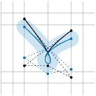
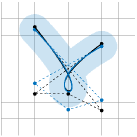
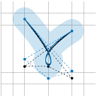
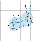
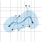
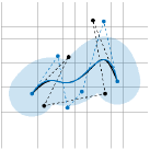
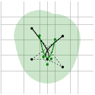
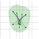
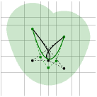
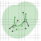
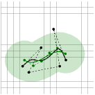
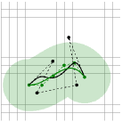
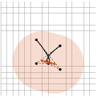
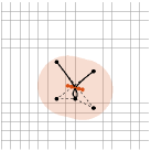
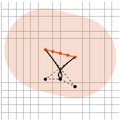
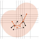
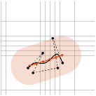
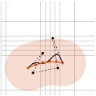
(a)	(b)	(c)	(d)	(e)	(f)

Figure 2: The maximum control-point distance defines a geometric bound on a Bézier curve (black) relative to another Bézier curve (blue, green, red), for example, its degree reduction. (top) Degree-one, (middle) degree-two and (bottom) degree-three reduction based on (a, d) Taylor reduction, (b, e) least squares reduction, (c, f) uniform matching reduction. Here, the reduced Bézier curves are elevated again to have the same number of control points.

III-B Hausdorff and Maximum Distances of Bézier Curves

As an alternative to norm-induced algebraic Bézier metrics, one can also compare Bezier curves based on set-theoretic distance measures as follows.

Definition 5

(Bézier Haussdorff & Maximum Distances) The Haussdorff and (parameterwise) maximum distances between two Bézier curves $\mathrm{B}_{\mathrm{p}_{0},\ldots,\mathrm{p}_{n}}(t)$ and $\mathrm{B}_{\mathrm{q}_{0},\ldots,\mathrm{q}_{m}}(t)$ over the unit interval $[0,1]$ are, respectively, defined as

$$\!d_{H}(\mathrm{B}_{\mathrm{p}_{0},\ldots,\mathrm{p}_{n}},\mathrm{B}_{\mathrm{q}_{0},\ldots,\mathrm{q}_{m}})$$

$$\hskip 11.38109pt:=\max\!\mathopen{}\mathclose{{}\left(\!\begin{array}[]{@{}c@{}}\max\limits_{t_{p}\in[0,1]}\min\limits_{t_{q}\in[0,1]}\|\mathrm{B}_{\mathrm{p}_{0},\ldots,\mathrm{p}_{n}}(t_{p})\!-\!\mathrm{B}_{\mathrm{q}_{0},\ldots,\mathrm{q}_{m}}(t_{q})\!\|,\\ \max\limits_{t_{q}\in[0,1]}\min\limits_{t_{p}\in[0,1]}\|\mathrm{B}_{\mathrm{p}_{0},\ldots,\mathrm{p}_{n}}(t_{p})\!-\!\mathrm{B}_{\mathrm{q}_{0},\ldots,\mathrm{q}_{m}}(t_{q})\!\|\end{array}\!}\right)\!\!,\!\!\!\!$$ (41)

$$\!d_{M}(\mathrm{B}_{\mathrm{p}_{0},\ldots,\mathrm{p}_{n}},\mathrm{B}_{\mathrm{q}_{0},\ldots,\mathrm{q}_{m}})\!\!:=\!\!\max_{t\in[0,1]}\!\|\mathrm{B}_{\mathrm{p}_{0},\ldots,\mathrm{p}_{n}}\!(t)\!-\!\mathrm{B}_{\mathrm{q}_{0},\ldots,\mathrm{q}_{m}}\!(t)\!\|.\!\!\!\!\!$$ (42)

Unfortunately, both the Haussdorff and maximum distances of Bézier curves do not accept an analytic solution in terms of control points in general, but can be analytically bounded above by the maximum distance of Bézier control points.

III-C Control-Point Distance of Bézier Curves

We introduce a new analytic Bézier metric that defines a relative geometric bound between Bézier curves, see Fig. 2.

Definition 6

(Bezier Control-Point Distance) The maximum control-point distance of $n^{\text{th}}$-order Bézier curves is defined as

$$d_{C}\mathopen{}\mathclose{{}\left(\mathrm{B}_{\mathrm{p}_{0},\ldots,\mathrm{p}_{n}},\mathrm{B}_{\mathrm{q}_{0},\ldots,\mathrm{q}_{n}}}\right):=\max_{i=0,\ldots,n}\|\mathrm{p}_{i}-\mathrm{q}_{i}\|.$$ (43)

Proposition 2

(Bézier Distance Order) The Frobenius, Hausdorff, and parameterwise & control-pointwise maximum distances of $n^{\text{th}}$-order Bézier curves satisfy

$$d_{H}(\mathrm{B}_{\mathrm{p}_{0},\ldots,\mathrm{p}_{n}},\mathrm{B}_{\mathrm{q}_{0},\ldots,\mathrm{q}_{n}}) \leq d_{M}(\mathrm{B}_{\mathrm{p}_{0},\ldots,\mathrm{p}_{n}},\mathrm{B}_{\mathrm{q}_{0},\ldots,\mathrm{q}_{n}}),$$ (44a)

$$\leq d_{C}(\mathrm{B}_{\mathrm{p}_{0},\ldots,\mathrm{p}_{n}},\mathrm{B}_{\mathrm{q}_{0},\ldots,\mathrm{q}_{n}}),$$ (44b)

$$\leq d_{F}(\mathrm{B}_{\mathrm{p}_{0},\ldots,\mathrm{p}_{n}},\mathrm{B}_{\mathrm{q}_{0},\ldots,\mathrm{q}_{n}}),$$ (44c)

$$\leq\sqrt{n}\,d_{C}(\mathrm{B}_{\mathrm{p}_{0},\ldots,\mathrm{p}_{n}},\mathrm{B}_{\mathrm{q}_{0},\ldots,\mathrm{q}_{n}}).$$ (44d)

Proof.

See Appendix E-F. ∎

Proposition 3

(Relative Bézier Bound) In the $d$-dimensional Euclidean space $\mathbb{R}^{d}$, an $n^{\text{th}}$-order Bézier curve is contained in the dilation of an another $n^{\text{th}}$-order Bézier curve by their maximum control-point distance, i.e.,

$$\mathrm{B}_{\mathrm{p}_{0},\ldots,\mathrm{p}_{n}}([0,1])$$

$$\subseteq\mathrm{B}_{\mathrm{q}_{0},\ldots,\mathrm{q}_{n}}([0,1])\oplus\mathcal{B}_{d}(d_{C}(\mathrm{B}_{\mathrm{p}_{0},\ldots,\mathrm{p}_{n}},\mathrm{B}_{\mathrm{q}_{0},\ldots,\mathrm{q}_{n}})\!)\!,$$ (45)

$$\subseteq\mathrm{conv}\mathopen{}\mathclose{{}\left(\mathrm{q}_{0},\ldots,\mathrm{q}_{n}}\right)\oplus\mathcal{B}_{d}(d_{C}(\mathrm{B}_{\mathrm{p}_{0},\ldots,\mathrm{p}_{n}},\mathrm{B}_{\mathrm{q}_{0},\ldots,\mathrm{q}_{n}})\!)\!,\!\!\!\!$$ (46)

where $\mathcal{B}_{d}(r):=\mathopen{}\mathclose{{}\left\{\mathrm{x}\in\mathbb{R}^{d}\big{|}\|\mathrm{x}\|\leq r}\right\}$ denotes the $d$-dimensional closed Euclidean ball of radius $r\geq 0$ centered at the origin.

Proof.

See Appendix E-G. ∎

The ordering (a.k.a. equivalence) relation of Bézier distances in Proposition 2 makes the maximum control-point distance a computationally efficient tool for discriminative comparison of Bézier curves independent of their degree $n$, whereas the Frobenius-norm distance tends to increase with increasing $n$. Moreover, similar to the convexity property in Property 3, the relative bound of Bézier curves via the maximum control-point distance in Proposition 3 offers an alternative way of constraining Bézier control points for safety and constraint verification in motion planning. We continue below with how different Bézier metrics behave under Bézier degree elevation and reduction operations.

IV Bezier Degree Elevation & Reduction

In this section, we briefly summarize the degree elevation and reduction operations of Bézier curves for (approximately) representing them with more or fewer control points. In particular, degree reduction is another building block of high-order Bézier approximations with multiple low-order Bézier segments. Accordingly, we introduce a new degree reduction method for approximating Bézier geometry more accurately.

IV-A Degree Elevation

Degree elevation generates an exact representation of Bézier curves with more control points, as illustrated in Fig. 3.

Definition 7

(Degree Elevation) A Bézier curve $\mathrm{B}_{\mathrm{q}_{0},\ldots,\mathrm{q}_{m}}$ of higher degree $m$ with control points $\mathrm{q}_{0},\ldots,\mathrm{q}_{m}$ is said to be the degree elevation of another Bézier curve $\mathrm{B}_{\mathrm{p}_{0},\ldots,\mathrm{p}_{n}}$ of lower degree $n\leq m$ with control points $\mathrm{p}_{0},\ldots,\mathrm{p}_{n}$ if and only if the curves are parameterwise identical, i.e.,

$$\mathrm{B}_{\mathrm{q}_{0},\ldots,\mathrm{q}_{m}}(t)=\mathrm{B}_{\mathrm{p}_{0},\ldots,\mathrm{p}_{n}}(t)\quad\forall t\in\mathbb{R}.$$ (47)

Bézier degree elevation can be analytically computed as:

Proposition 4

(Elevated Control Points) A Bézier curve $\mathrm{B}_{\mathrm{q}_{0},\ldots,\mathrm{q}_{m}}$ of degree $m$ is the degree elevation of a Bézier curve $\mathrm{B}_{\mathrm{p}_{0},\ldots,\mathrm{p}_{n}}$ of degree $n\leq m$ if and only if the control point matrices $\mathbf{Q}_{m}=\mathopen{}\mathclose{{}\left[\mathrm{q}_{0},\ldots,\mathrm{q}_{m}}\right]$ and $\mathbf{P}_{n}=\mathopen{}\mathclose{{}\left[\mathrm{p}_{0},\ldots,\mathrm{p}_{n}}\right]$ satisfy

$$\mathbf{Q}_{m}=\mathbf{P}_{n}\mathbf{E}(n,m),$$ (48)

where the degree elevation matrix $\mathbf{E}(n,m)$ is defined as

$$\mathbf{E}(n,m):=\mathbf{T}_{\mathrm{m}}^{\mathrm{b}}(n)\mathbf{I}_{(n+1)\times(m+1)}\mathbf{T}_{\mathrm{b}}^{\mathrm{m}}(m),$$ (49)

and $\mathbf{I}_{n+1\times(m+1)}$ is the $(n+1)\times(m+1)$ rectangular identify matrix with ones in the main diagonal and zeros elsewhere.

Proof.

See Appendix E-H. ∎

Observe that (49) leverages the change of basis between Bernstein and monomial bases because degree elevation of monomial curves is trivial.

Higher-order Bernstein basis vectors can also be obtained from lower ones via degree elevation, which offers another way of determining the elevation matrix.

Proposition 5

(Elevated Bernstein Basis) For any $n\leq m$, the elevation matrix $\mathbf{E}(n,m)$ relates Bernstein basis vectors as

$$\mathrm{b}_{n}(t)=\mathbf{E}(n,m)\mathrm{b}_{m}(t)\quad\forall t\in\mathbb{R}.$$ (50)

Hence, $\mathbf{E}(n,m)$ can be determined as

$$\mathbf{E}(n,m)=\mathbf{b}_{n}(t_{0},\ldots,t_{m})\mathbf{b}_{m}(t_{0},\ldots,t_{m})^{-1},$$ (51)

where $t_{0},\ldots,t_{m}\in\mathbb{R}$ are an arbitrary selection of pairwise distinct curve parameters, i.e., $t_{i}\neq t_{j}$ for all $i\neq j$.

Proof.

See Appendix E-I. ∎

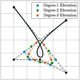
Figure 3: Degree elevation represents Bézier curves exactly by more control points that asymptotically converge to the curve itself as the amount of degree elevation goes to infinity.

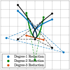
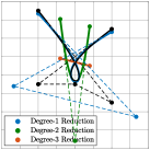
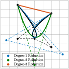
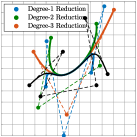
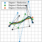
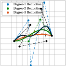
(a)	(b)	(c)	(d)	(e)	(f)

Figure 4: Degree reduction approximately represents Bézier curves with fewer control points. (a, d) Taylor degree reduction with a Taylor offset $t_{o}=0.5$, (b, e) Least squares reduction, (c, f) Uniform matching reduction with uniformly spaced parameters $t_{0},\ldots,t_{m}$ over the unit interval, i.e., $t_{i}=\frac{i}{m}$ for $i=0,\ldots,m$.

In fact, the elements of the degree elevation matrix can be determined explicitly [45, 44]:

Proposition 6

(Elevation Matrix Elements) For any $n\leq m$, the elements of the elevation matrix $\mathbf{E}(n,m)$ are given by

$$\mathopen{}\mathclose{{}\left[\mathbf{E}(n,m)}\right]_{i+1,j+1}=\mathopen{}\mathclose{{}\left\{\begin{array}[]{@{}c@{\,\,}l@{}}\frac{\binom{n}{i}\binom{m-n}{j-i}}{\binom{m}{j}}&\text{, if }m-n\geq j-i\geq 0\\ 0&\text{, otherwise,}\end{array}}\right.$$ (54)

where $i=0,\ldots,n$ and $j=0,\ldots,m$.

Proof.

See Appendix E-J. ∎

IV-A1 Important Elevation Matrix Properties

The degree elevation matrices are full rank and have unit column sum [45].

Proposition 7

(Full Rank Elevation Matrix) For any $n\leq m$, the elevation matrix $\mathbf{E}(n,m)\in\mathbb{R}^{(n+1)\times(m+1)}$ is full rank of $n+1$, i.e., $\mathrm{rank}(\mathbf{E}(n,m))=n+1$.

Proof.

See Appendix E-K. ∎

Proposition 8

(Elevation Matrix Row & Column Sum) For any $n\leq m$, the sum of each column of the elevation matrix $\mathbf{E}(n,m)$ is one, whereas each of its rows sums to $\frac{m+1}{n+1}$, i.e.,

$$\mathbf{1}_{1\times(n+1)}\,\mathbf{E}(n,m) =\mathbf{1}_{1\times(m+1)},$$ (55a)

$$\mathbf{E}(n,m)\mathbf{1}_{(m+1)\times 1} =\tfrac{m+1}{n+1}\mathbf{1}_{(n+1)\times 1}.$$ (55b)

where $\mathbf{1}_{n\times m}$ denotes the $n\times m$ matrix of all ones.

Proof.

See Appendix E-L. ∎

IV-A2 Bézier Metrics under Degree Elevation

Different Bézier metrics behave differently under degree elevation: while the L2-norm distance stays constant, the Frobenius norm distance might increase, whereas the maximum control-point distance is nonincreasing under elevation.

Proposition 9

(Invariance of Bézier L2-norm distance under degree elevation) The L2-norm distance of Bézier curves, $\mathrm{B}_{\mathrm{p}_{0},\ldots,\mathrm{p}_{n}}(t)$ and $\mathrm{B}_{\mathrm{q}_{0},\ldots,\mathrm{q}_{m}}(t)$ over the unit interval $[0,1]$, are preserved under degree elevation, i.e.,

$$d_{L2}(\mathrm{B}_{\mathopen{}\mathclose{{}\left[\mathrm{p}_{0},\ldots,\mathrm{p}_{n}}\right]\mathbf{E}(n,k)},\mathrm{B}_{\mathopen{}\mathclose{{}\left[\mathrm{q}_{0},\ldots,\mathrm{q}_{m}}\right]\mathbf{E}(m,h)}\!) =d_{L2}(\mathrm{B}_{\mathrm{p}_{0},\ldots,\mathrm{p}_{n}},\mathrm{B}_{\mathrm{q}_{0},\ldots,\mathrm{q}_{m}}),$$ (56)

for any $k\geq n$ and $h\geq m$.

Proof.

See Appendix E-M. ∎

Proposition 10

(Elevated Frobenius Distance) Under degree elevation, the Frobenius distance of $n^{\text{th}}$-order Bézier curves satisfies for any $m\geq n\in\mathbb{N}$ that

$$d_{F}(\mathrm{B}_{[\mathrm{p}_{0},\ldots,\mathrm{p}_{n}]\mathbf{E}(n,m)},\mathrm{B}_{[\mathrm{q}_{0},\ldots,\mathrm{q}_{n}]\mathbf{E}(n,m)})^{2}$$

$$\hskip 91.04881pt\leq\tfrac{m+1}{n+1}d_{F}(\mathrm{B}_{\mathrm{p}_{0},\ldots,\mathrm{p}_{n}},\mathrm{B}_{\mathrm{q}_{0},\ldots,\mathrm{q}_{n}})^{2}.$$ (57)

Proof.

See Appendix E-N. ∎

Proposition 11

(Nonincreasing Elevated Control-Point Distance) The maximum control-point distance of $n^{\text{th}}$-order Bézier curves is non-increasing under degree elevation, i.e.,

$$d_{C}(\mathrm{B}_{\mathopen{}\mathclose{{}\left[\mathrm{p}_{0},\ldots,\mathrm{p}_{n}}\right]\mathbf{E}(n,m)},\mathrm{B}_{\mathopen{}\mathclose{{}\left[\mathrm{q}_{0},\ldots,\mathrm{q}_{n}}\right]\mathbf{E}(n,m)})\leq d_{C}(\mathrm{B}_{\mathrm{p}_{0},\ldots,\mathrm{p}_{n}},\mathrm{B}_{\mathrm{q}_{0},\ldots,\mathrm{q}_{n}}),$$ (58)

for any $m\geq n\in\mathbb{N}$.

Proof.

See Appendix E-O. ∎

Thus, the ordering relation of Bézier distances in Proposition 2, the relative geometric bound of Bézier curves in Proposition 3, and the nonincreasing property under degree elevation in Proposition 11 make the maximum control-point distance an analytic and intuitive metric for comparing Bézier curves.

Finally, it is useful to note that as elevation degree goes to infinity, one has all Bézier curve points as its control points.

Proposition 12 ([44])

(Asymptotic Behavior of Degree Elevation) As the elevation degree goes to infinity, the elevated Bézier control points become the Bézier curve points, i.e.,

$$\lim_{m\rightarrow\infty}[\mathrm{p}_{0},\ldots,\mathrm{p}_{n}]\mathbf{E}(n,m)=\mathopen{}\mathclose{{}\left[\mathrm{B}_{\mathrm{p}_{0},\ldots,\mathrm{p}_{n}}(t)}\right]_{0\leq t\leq 1}\,.$$ (59)

IV-B Degree Reduction

As opposed to degree elevation, Bézier degree reduction aims to approximately represent a Bézier curve with fewer control points, as illustrated in Fig. 4. Hence, degree reduction is naturally defined as the inverse of degree elevation.^IV-B

Definition 8

(Degree Reduction) A Bézier curve $\mathrm{B}_{\mathrm{q}_{0},\ldots,\mathrm{q}_{m}}$ of lower degree $m$ with control points $\mathbf{Q}_{m}=\mathopen{}\mathclose{{}\left[\mathrm{q}_{0},\ldots,\mathrm{q}_{m}}\right]$ is said to be a degree reduction of another Bézier curve $\mathrm{B}_{\mathrm{p}_{0},\ldots,\mathrm{p}_{n}}$ of higher degree $n\geq m$ with control points $\mathbf{P}_{n}=\mathopen{}\mathclose{{}\left[\mathrm{p}_{0},\ldots,\mathrm{p}_{n}}\right]$ if and only if the control points are related to each other by

$$\mathbf{Q}_{m}=\mathbf{P}_{n}\mathbf{R}(n,m),$$ (60)

where $\mathbf{R}(n,m)\!\in\!\mathbb{R}^{(n+1)\times(m+1)}$ denotes a degree reduction matrix that is a right inverse of the elevation matrix $\mathbf{E}(m,n)$, i.e.,

$$\mathbf{E}(m,n)\mathbf{R}(n,m)=\mathbf{I}_{(m+1)\times(m+1)}.$$ (61)

That is to say, the degree elevation from $m$ to $n$ followed by a degree reduction from $n$ to $m$ preserves Bézier curves; but, the reverse is not correct in general. Also note that the right inverse of the elevation matrix is not unique, which allows many alternative ways of constructing a reduction matrix.

IV-B1 Least Squares Reduction

A standard choice for degree reduction is the pseudo-inverse of the elevation matrix [44].

Definition 9

(Least Squares Reduction) The least squares reduction matrix $\mathbf{R}_{L2}(n,m)$ is defined as the pseudo-inverse of the elevation matrix $\mathbf{E}(m,n)$ that is explicitly given by

$$\mathbf{R}_{L2}(n,m)={\mathbf{E}(m,n)}^{\mathrm{T}}(\mathbf{E}(m,n){\mathbf{E}(m,n)}^{\mathrm{T}})^{-1}.$$ (62)

Note that $\mathbf{E}(m,n){\mathbf{E}(m,n)}^{\mathrm{T}}$ is invertible for any $m\leq n\in\mathbb{N}$ because $\mathbf{E}(m,n)$ is full rank (Proposition 7), which implies $\mathbf{E}(m,n)\mathbf{R}_{L2}(n,m)=\mathbf{I}_{(m+1)\times(m+1)}$. An example of least squares reduction is presented in 4(b,e), where the Bézier end-points are not preserved after degree reduction.

The least squares degree reduction is known to be optimal in the sense of the L2- and Frobenius-norm distances [45, 52].

Proposition 13

(Optimality of Least Squares Reduction) With respect to the L2-norm and Frobenius-norm distances, the optimal $m^{\text{th}}$-order Bezier curve $\mathrm{B}_{\mathrm{q}_{0},\ldots,\mathrm{q}_{m}}(t)$ with control points $\mathbf{Q}_{m}=[\mathrm{q}_{0},\ldots,\mathrm{q}_{m}]$ that is closest to a higher $\text{n}^{\text{th}}$-order Bézier curve $\mathrm{B}_{\mathrm{p}_{0},\ldots,\mathrm{p}_{n}}(t)$ with control points $\mathbf{P}_{m}=\mathopen{}\mathclose{{}\left[\mathrm{p}_{0},\ldots,\mathrm{p}_{n}}\right]$ is given by the least squares reduction, i.e.,

$$\mathbf{Q}_{m} =\operatornamewithlimits{argmin}_{\mathrm{q}_{0},\ldots,\mathrm{q}_{m}\in\mathbb{R}^{d}}d_{L2}(\mathrm{B}_{\mathrm{p}_{0},\ldots,\mathrm{p}_{n}},\mathrm{B}_{\mathopen{}\mathclose{{}\left[\mathrm{q}_{0},\ldots,\mathrm{q}_{m}}\right]\mathbf{E}(m,n)}),$$ (63a)

$$=\operatornamewithlimits{argmin}_{\mathrm{q}_{0},\ldots,\mathrm{q}_{m}\in\mathbb{R}^{d}}d_{F}(\mathrm{B}_{\mathrm{p}_{0},\ldots,\mathrm{p}_{n}},\mathrm{B}_{\mathopen{}\mathclose{{}\left[\mathrm{q}_{0},\ldots,\mathrm{q}_{m}}\right]\mathbf{E}(m,n)}),$$ (63b)

$$=\mathbf{P}_{n}\mathbf{R}_{L2}(n,m).$$ (63c)

Proof.

See Appendix E-P. ∎

IV-B2 Taylor Reduction

Another classical degree reduction is Taylor approximation that preserves local derivatives.

Definition 10

(Taylor Reduction) The Taylor reduction matrix $\mathbf{R}_{\mathrm{\tau},t_{o}}(n,m)$ for approximating an $n^{\text{th}}$-order Bezier curve around $t_{o}\in\mathbb{R}$ by a lower $m^{\text{th}}$-order Bezier curve is defined as

$$\mathbf{R}_{\mathrm{\tau},t_{o}}(n,m):=\mathbf{T}_{\mathrm{\tau}}^{\mathrm{b}}(n,t_{o})\mathbf{I}_{(n+1)\times(m+1)}\mathbf{T}_{\mathrm{b}}^{\mathrm{\tau}}(m,t_{o}),$$ (64)

where $\mathbf{T}_{\mathrm{\tau}}^{\mathrm{b}}$ and $\mathbf{T}_{\mathrm{b}}^{\mathrm{\tau}}$ are the Taylor-to-Bernstein and the Bern-stein-to-Taylor basis transformation matrices in Lemma 2.

In other words, Taylor reduction perform a basis transformation from Bernstein to Taylor basis, and ignores some higher-order Taylor basis elements, and then comes back to Bernstein basis. Hence, it has a strong bias and local expressiveness around the Taylor offset $t_{o}$, as illustrated in Fig. 4(a,d).

Proposition 14

(Taylor Reduction as Elevation Inverse) The Taylor reduction matrix $\mathbf{R}_{\mathrm{\tau},t_{o}}(n,m)$ is a right inverse of the elevation matrix $\mathbf{E}(m,n)$, i.e., for any $m\leq n\in\mathbb{N}$

$$\mathbf{E}(m,n)\mathbf{R}_{\mathrm{\tau},t_{o}}(n,m)=\mathbf{I}_{(m+1)\times(m+1)}.$$ (65)

Proof.

See Appendix E-Q. ∎

It is important to observe in Fig. 4 that both the least-squares and Taylor reduction methods offer less freedom in controlling the resulting shape of Bézier approximations; for example, the end points of the original curve are not preserved after degree reduction, which is essential for path smoothing with boundary conditions [14].

IV-B3 Parameterwise Matching Reduction

In order to accurately approximate curve shape and geometry, we propose a new parameterwise matching reduction method that preserves a finite set of curve points after degree reduction.

Definition 11

(Parameterwise Matching Reduction) For Bézier degree reduction from a higher degree $n$ to a lower degree $m\leq n$, the parameterwise matching degree reduction matrix $\mathbf{R}_{t_{0},\ldots,t_{m}}(n,m)$ associated with pairwise distinct parameters $t_{0},\ldots,t_{m}\in\mathbb{R}$ (i.e., $t_{i}\neq t_{j}$ for all $i\neq j$) is defined as

$$\mathbf{R}_{t_{0},\ldots,t_{m}}(n,m):=\mathbf{b}_{n}(t_{0},\ldots,t_{m})\mathbf{b}_{m}(t_{0},\ldots,t_{m})^{-1},$$ (66)

where $\mathbf{b}_{n}(t_{0},\ldots,t_{m})$ is the Bernstein basis matrix in (28).

For example, a numerically stable choice of $t_{0},\ldots,t_{m}$ over the unit interval is the uniformly spaced parameters in $[0,1]$, i.e., $t_{i}=\frac{i}{m}$ for $i=0,\ldots,m$. We call the corresponding reduction operation as the uniform matching reduction.

As expected, the parameterwise matching reduction of Bézier curves keeps curve points unchanged at $t_{0},\ldots,t_{m}$.

Proposition 15

(Preserved Points of Matching Reduction) For any pairwise distinct $t_{0},\ldots,t_{m}\in\mathbb{R}$, a Bézier curve $\mathrm{B}_{\mathrm{p}_{0},\ldots,\mathrm{p}_{n}}(t)$ of degree $n$ and its parameterwise matching reduction $\mathrm{B}_{\mathrm{q}_{0},\ldots,\mathrm{q}_{m}}(t)$ of degree $m\leq n$ with control points

$$[\mathrm{q}_{0},\ldots,\mathrm{q}_{m}]=[\mathrm{p}_{0},\ldots,\mathrm{p}_{n}]\mathbf{R}_{t_{0},\ldots,t_{m}}(n,m)$$ (67)

match at the curve parameters $t_{0},\ldots,t_{m}$, i.e.,

$$\mathrm{B}_{\mathrm{q}_{0},\ldots,\mathrm{q}_{m}}(t)=\mathrm{B}_{\mathrm{p}_{0},\ldots,\mathrm{p}_{n}}(t)\quad\forall t=t_{0},\ldots,t_{m}.$$ (68)

Proof.

See Appendix E-R. ∎

Proposition 16

(Matching Reduction as Elevation Inverse) For any $m\leq n$ and pairwise distinct reals $t_{0},\ldots,t_{m}\in\mathbb{R}$, the parameterwise matching degree matrix $\mathbf{R}_{t_{0},\ldots,t_{m}}(n,m)$ is a right inverse of the elevation matrix $\mathbf{E}(m,n)$,

$$\mathbf{E}(m,n)\mathbf{R}_{t_{0},\ldots,t_{m}}(n,m)=\mathbf{I}_{(m+1)\times(m+1)}.$$ (69)

Proof.

See Appendix E-S ∎

Taylor Reduction
Least Squares
Uniform Matching
	$2(n-1)$ Linear Segments	$4(n-1)$ Linear Segments	$6(n-1)$ Linear Segments	$(n-1)$ Quad Segments	$2(n-1)$ Quad Segments	$3(n-1)$ Quad Segments
	(a)	(b)	(c)	(d)	(e)	(f)

Figure 5: Approximation of a Bézier curve of degree $n=8$ by (a, b, c) linear and (d, e, f) quadratic Bézier segments using (top) Taylor, (middle) least squares, and (bottom) uniform matching reduction. The Taylor offset is set to be 0.5, and a uniform partition of the unit interval is used with (a) $2(n-1)$, (b) $4(n-1)$, (c) $6(n-1)$ partition elements for linear approximations, and (d) $(n-1)$, (e) $2(n-1)$, (f) $3(n-1)$ partition elements for quadratic approximations. Bézier approximation rule: An $n^{\text{th}}$-order Bézier curve can be approximated accurately by $3(n-1)$ quadratic and $6(n-1)$ linear uniform matching Bézier curves.

Another interesting connection between degree elevation and matching reduction is their shared matrix form.

Proposition 17

(Shared Form of Matching Reduction and Elevation Matrix) For any $n,m\in\mathbb{N}$ and any pairwise distinct reals $t_{0},\ldots,t_{m}\in\mathbb{R}$, the Bernstein basis matrices satisfy

$$\!\!\!\mathbf{b}_{n}(t_{0},\ldots,t_{m})\mathbf{b}_{m}(t_{0},\ldots,t_{m})^{-1}\!\!=\!\!\mathopen{}\mathclose{{}\left\{\begin{array}[]{@{}c@{}l@{}}\mathbf{E}(n,m)&\text{, if }n\leq m,\\ \!\mathbf{R}_{t_{0},\ldots,t_{m}}\!(n,m)&\text{, if }n\geq m,\end{array}}\right.\!\!\!\!$$ (72)

where $\mathbf{E}(n,n)=\mathbf{R}_{t_{0},\ldots,t_{m}}(n,n)=\mathbf{I}_{(n+1)\times(n+1)}$.

Proof.

It follows from Proposition 5 and Definition 11. ∎

A critical property of matching reduction is that the degree-one reduction error can be determined analytically.

Proposition 18

(Degree-One Matching Reduction Error) For any pairwise distinct $t_{0},\ldots t_{n}\in\mathbb{R}$, the difference between a Bézier curve $\mathrm{B}_{\mathrm{p}_{0},\ldots,\mathrm{p}_{n+1}}(t)$ and its parameterwise matching degree reduction $\mathrm{B}_{\mathrm{q}_{0},\ldots,\mathrm{q}_{n}}(t)$, with control points

$$[\mathrm{q}_{0},\ldots,\mathrm{q}_{n}]=[\mathrm{p}_{0},\ldots,\mathrm{p}_{n+1}]\mathbf{R}_{t_{0},\ldots,t_{n}}(n+1,n),$$ (73)

is given by

$$\mathrm{B}_{\mathrm{p}_{0},\ldots,\mathrm{p}_{n+1}}(t)-\mathrm{B}_{\mathrm{q}_{0},\ldots,\mathrm{q}_{n}}(t)=\Delta\mathrm{p}\prod_{i=0}^{n}(t-t_{i}),$$ (74)

where

$$\Delta\mathrm{p}=\sum_{i=0}^{n+1}(-1)^{n+1-i}\scalebox{1.2}{$\binom{n+1}{i}$}\mathrm{p}_{i}.$$ (75)

Proof.

See Appendix E-T. ∎

It is important to observe that the degree-one matching reduction difference vector $\Delta\mathrm{p}$ is independent of the selection of matching parameters $t_{0},\ldots,t_{n}$ where the reduction error is zero. Moreover, the polynomial product form of the degree-one matching reduction error, illustrated in Fig. 6, plays a key role in determining how many local low-order Bézier segments are needed for approximating high-order Bézier curves accurately, as discussed below in Section V.

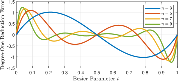
Figure 6: Scaled degree-one reduction error function $\varepsilon_{n}(t)$ for uniform matching reduction of Bézier curves that is defined as $\varepsilon_{n}(t)=\frac{\prod_{i=0}^{n}t-\frac{i}{n}}{\prod_{i=0}^{n}\frac{1}{2n}-\frac{i}{n}}$.

V Adaptive Degree Reduction and Splitting
of Bézier Curves

In this section, we consider the problem of approximating high-order Bézier curves by multiple lower-order Bézier segments. We first describe how Bézier approximations can be performed over a given finite partition of the unit interval, and then propose linear and binary search methods for adaptive approximation of high-order Bézier curves by lower-order Bézier segments at any desired accuracy level. We also present a rule of thumb for accurate Bézier discretization.

V-A Bézier Approximation over a Partition of the Unit Interval

Consider an $n^{\text{th}}$-order Bézier curve $\mathrm{B}_{\mathrm{p}_{0},\ldots,\mathrm{p}_{n}}(t)$ with control points $\mathbf{P}_{n}=[\mathrm{p}_{0},\ldots,\mathrm{p}_{n}]$ defined over the unit interval $[0,1]$. Suppose $T=[t_{0},\ldots,t_{k}]$ is an ordered list of distinct parameters that defines a partition of the unit interval into $k$ splits, i.e., $0=t_{0}<t_{1}<\ldots<t_{k-1}<t_{k}=1$. Accordingly, the Bézier curve $\mathrm{B}_{\mathrm{p}_{0},\ldots,\mathrm{p}_{n}}(t)$ can be locally approximated over each parameter subinterval $[t_{i-1},t_{i}]$ by a lower $m^{\text{th}}$-order Bezier curve $\mathrm{B}_{\mathrm{q}_{0,i},\ldots,\mathrm{q}_{m,i}}(t)$ whose control points $\mathbf{Q}_{m,i}=[\mathrm{q}_{0,i},\ldots,\mathrm{q}_{m,i}]$ is obtained based on a choice of a degree reduction matrix $\mathbf{R}(n,m)$ (see Definition 8) as

$$\mathbf{Q}_{m,i}=\mathrm{DegreeReduction}(\mathbf{P}_{n,i},m):=\mathbf{P}_{n,i}\mathbf{R}(n,m),$$ (76)

using the reparametrization $\mathrm{B}_{\mathrm{p}_{0,i},\ldots,\mathrm{p}_{n,i}}(t)$ of $\mathrm{B}_{\mathrm{p}_{0},\ldots,\mathrm{p}_{n}}(t)$ from $[t_{i-1},t_{i}]$ to the unit interval $[0,1]$ with new control points $\mathbf{P}_{n,i}=[\mathrm{p}_{0,i},\ldots,\mathrm{p}_{n,i}]$ (see Lemma 4) that are obtained as

$$\,\mathbf{P}_{n,i} =\mathrm{Reparameterize}(\mathbf{P}_{i},[t_{i-1},t_{i}]),$$ (77)

$$:=\mathbf{b}_{n}\mathopen{}\mathclose{{}\left(0,\tfrac{1}{n},\ldots,\tfrac{n-1}{n},1}\right)\mathbf{b}_{n}\mathopen{}\mathclose{{}\left(s_{i}(0),s_{i}(\tfrac{1}{n}),\ldots,s_{i}(\tfrac{n-1}{n}),s_{i}(1)\!}\right)^{\!-1}\!\!\!,$$ (78)

where $s_{i}(t)=\mathrm{B}_{t_{i-1},t_{i}}(t)=t_{i-1}(1-t)+t_{i}\,t$ is the Bézier parameter scaling function. Hence, as described in Algorithm 1, the high-order Bézier curve $\mathrm{B}_{\mathrm{p}_{0},\ldots,\mathrm{p}_{n}}([0,1])$ can be approximated by a collection of low-order Bézier segments $\mathrm{B}_{\mathrm{q}_{0,i},\ldots,\mathrm{q}_{m,i}}([0,1])$ constructed over each partition element $[t_{i-1},t_{i}]$ such that $\mathrm{B}_{\mathbf{Q}_{m,i}}([0,1])$ approximates $\mathrm{B}_{\mathbf{P}_{n}}([t_{i-1},t_{i}])$.

Input: $\mathbf{P}_{n}\in\mathbb{R}^{d\times n}$: Bezier Control Points

          $m\in\mathbb{N}$: Reduction Degree

          $T=[t_{0},\ldots,t_{k}]$: Partition of the Unit Interval

Output: $\mathbf{Q}_{m,1},\ldots\mathbf{Q}_{m,k}$: List of Reduced Control Points

           where $\mathrm{B}_{\mathbf{Q}_{m,i}}([0,1])$ approximates $\mathrm{B}_{\mathbf{P}_{n}}([t_{i-1},t_{i}])$

3 $k\leftarrow\mathrm{length}(T)-1$ // Number of Segments

4 for $i\leftarrow 1$ to $k$ do

5       $\mathbf{P}_{n,i}\leftarrow\textrm{Reparametrize}(\mathbf{P}_{n},[t_{i-1},t_{i}])$

6       $\mathbf{Q}_{m,i}\leftarrow\textrm{DegreeReduction}(\mathbf{P}_{n,i},m)$

7      

return $\mathbf{Q}_{m,1},\ldots,\mathbf{Q}_{m,k}$

                 of the Unit Interval

Algorithm 1 Bézier Approximation over a Partition

                 of the Unit Interval

In Fig. 5, we illustrate approximating an $8^{\text{th}}$-order Bézier curve with linear and quadratic Bézier segments over the uniform partitions of the unit interval using Taylor, least squares, and uniform matching reductions. As seen in Fig. 5, the uniform matching reduction performs better in approximately representing the original curve shape than the least squares reduction which performs better than Taylor reduction. Also notice that the end points of the original curve are kept unchanged only under the uniform matching reduction.

V-B Bézier Approximation Rule

A practical question of approximating high-order Bézier curves by a finite number of low-order Bézier segments is what the required number of local Bézier segments is for an accurate Bézier discretization. As expected, the answer depends on the desired level of approximation accuracy and the degree of Bézier curves. In this part, we provide an answer based on the structural form of the Bézier approximation error of degree-one matching reduction (Proposition 18), and the numerical analysis of Bézier approximations in Section VI.

A Rule of Thumb for Bézier Approximations

An $n^{\text{th}}$-order Bézier curve can be accurately approximated by $3(n-1)$ quadratic and $6(n-1)$ linear Bézier curves obtained via uniform matching reduction.

According to Proposition 18, an $n^{\text{th}}$-order Bézier curve can be written as the sum of an $(n-1)^{\text{th}}$-order reduced Bézier curve and a degree-one matching reduction error which is a polynomial of order $n$ in the product form. Note that the $(n-1)^{\text{th}}$-order reduced Bézier curve can be better approximated with the same number of low-order Bézier segments than the original $n^{\text{th}}$-order Bézier curve. Hence, one can determine the required number of low-order Bézier segments for accurately approximating high-order Bézier curves by exploiting the functional form of the reduction error. As seen in Fig. 6, the degree-one matching reduction error of $n^{\text{th}}$-order Bézier curves has $(n-1)$ extreme (local maximum and minimum) points. This implies that a proper approximation of $n^{\text{th}}$-order Bézier curves structurally requires at least $(n-1)$ quadratic Bézier curves which has a single extremum. Because of the asymmetry of the approximation error around each extreme point, one needs at least $2(n-1)$ quadratic segments. Since the uniform matching reduction uses uniformly spaced parameters for approximation, we observe in our numerical studies in Section VI that the asymmetry around each extreme point can be better handled with $3(n-1)$ quadratic patches in practice. Our numerical analysis also shows that approximating $n^{\text{th}}$-order Bézier curves by $3(n-1)$ quadratic segments ensures a normalized (i.e., scale invariant) approximation error below the order of $10^{-3}$ for computing important curve features such as curve length, distance-to-point/line, and maximum velocity/acceleration. Similarly, since a quadratic polynomial structurally requires at least two linear curve segments for a proper representation of its unique extremum, we also observe from our numerical studies that approximating $n^{\text{th}}$-order Bézier curves by $6(n-1)$ linear Bézier segments yields a normalized approximation error in the order of $10^{-3}$.

Input: $\mathbf{P}_{n}\in\mathbb{R}^{d\times n}$: Bezier Control Points

          $m\in\mathbb{N}$: Reduction Degree

          $\varepsilon>0$: Approximation Tolerance

Output: $T=[t_{0},\ldots,t_{k}]$: Split Intervals

           $\mathbf{Q}_{m,1},\ldots\mathbf{Q}_{m,k}$: List of Reduced Control Points

           where $\mathrm{B}_{\mathbf{Q}_{m,i}}([0,1])$ approximates $\mathrm{B}_{\mathbf{P}_{n}}([t_{i-1},t_{i}])$

1 $k\leftarrow 1$ // Number of Segments

2 $T\leftarrow[0,1]$ // Initial Partition

3 while $k<\mathrm{length}(T)$ do

4       for $i\leftarrow 1$ to $k$ do

5             $\mathbf{P}_{n,i}\leftarrow\textrm{Reparametrize}(\mathbf{P}_{n},[t_{i-1},t_{i}])$

6             $\mathbf{Q}_{m,i}\leftarrow\textrm{DegreeReduction}(\mathbf{P}_{n,i},m)$

7             if $\mathrm{BezierDistance}(\mathbf{P}_{n,i},\mathbf{Q}_{m,i}\mathbf{E}(m,n))>\varepsilon$ then

8                   $T\leftarrow[0,\frac{1}{k+1},\ldots,\frac{k}{k+1},1]$

9                   break

10            

11      $k\leftarrow k+1$

12      

13$k\leftarrow\mathrm{length}(T)-1$ // Number of Segments

14 return $T,\mathbf{Q}_{m,1},\ldots,\mathbf{Q}_{m,k}$

Algorithm 2 Adaptive Degree Reduction and Splitting via Linear Search

Input: $\mathbf{P}_{n}\in\mathbb{R}^{d\times n}$: Bezier Control Points

          $m\in\mathbb{N}$: Reduction Degree

          $\varepsilon>0$: Approximation Tolerance

Output: $T=[t_{0},\ldots,t_{k}]$: Split Intervals

           $\mathbf{Q}_{m,1},\ldots\mathbf{Q}_{m,k}$: List of Reduced Control Points

           where $\mathrm{B}_{\mathbf{Q}_{m,i}}([0,1])$ approximates $\mathrm{B}_{\mathbf{P}_{n}}([t_{i-1},t_{i}])$

1

2$k\leftarrow 1$ // Segment Counter

3 $T\leftarrow[0,1]$ // Initial Partition

4 while $k<\mathrm{length}(t)$ do

5       $\mathbf{P}_{n,k}\leftarrow\textrm{Reparametrize}(\mathbf{P}_{n},[t_{k-1},t_{k}])$

6       $\mathbf{Q}_{m,k}\leftarrow\textrm{DegreeReduction}(\mathbf{P}_{n,i},m)$

7       if $\mathrm{BezierDistance}(\mathbf{P}_{n,k},\mathbf{Q}_{m,k}\mathbf{E}(m,n))>\varepsilon$ then

8             $T\leftarrow[t_{0},\ldots,t_{k-1},\frac{t_{k-1}+t_{k}}{2},t_{k}]$

9      else

10             $k\leftarrow k+1$

11      

12$k\leftarrow\mathrm{length}(T)-1$ // Number of Segments

return $T,\mathbf{Q}_{m,1},\ldots,\mathbf{Q}_{m,k}$

Algorithm 3 Adaptive Degree Reduction and Splitting via Binary Search

V-C Adaptive Bézier Approximation via Bézier Metrics

The Bézier approximation rule above holds for any Bézier curve in general, and ensures a proper structural representation of high-order Bézier curves at a certain level of accuracy. However, high-order Bézier curves might have redundant control points, for example, consider the degree elevation of Bézier curves in Fig. 3, and also different application settings might require different levels of approximation accuracy. Hence, it is desirable to perform Bézier approximation that is tailored to individual Bézier curves and can adaptively select the required number of Bézier segments and the partition of the unit interval based on the desired level of accuracy. In this part, we extend Bézier approximations over a given partition of the unit interval by incorporating a search strategy to automatically determine a partition of the unit interval in order to achieve a desired level of measurable approximation accuracy.

Linear Srch $\varepsilon=.5$
Linear Srch $\varepsilon=.1$
Binary Srch $\varepsilon=.1$
	Linear Taylor Reduction	Linear Least Squares	Linear Uniform Matching	Quadratic Taylor Reduction	Quadratic Least Squares	Quadratic Uniform Matching
	(a)	(b)	(c)	(d)	(e)	(f)

Figure 7: Adaptive approximation of a $8^{\text{th}}$-order Bézier curve (black dashed line) by (a, b, c) linear and (d, e, f) quadratic Bézier curve segments (red and blue patches) that are automatically obtained via (top, middle) linear and (bottom) binary search based on (a, d) Taylor approximation, (b, e) least squares reduction, and (c, f) uniform matching reduction. The Bézier splitting is automatically done based on a desired approximation tolerance $\varepsilon>0$ specified in term of the Bézier maximum control-point distance: (top) $\varepsilon=0.5$ units, (middle, bottom) $\varepsilon=0.1$ units.

As discussed in Section V-A, an $n^{\text{th}}$-order Bézier curve $\mathrm{B}_{\mathrm{p}_{0},\ldots,\mathrm{p}_{n}}(t)$ can be locally approximated by $m^{\text{th}}$-order Bezier segments over each element of a $k$-partition $T=[t_{0},\ldots,t_{k}]$ of the unit interval by applying curve reparametrization and degree reduction as

$$\mathbf{P}_{n,i} =\mathrm{Reparameterize}(\mathbf{P}_{i},[t_{i-1},t_{i}]),$$ (79)

$$\mathbf{Q}_{m,i} =\mathrm{DegreeReduction}(\mathbf{P}_{n,i},m),$$ (80)

Hence, one can measure the quality of approximating $\mathrm{B}_{\mathrm{p}_{0,i},\ldots,\mathrm{p}_{n,i}}(t)$ by $\mathrm{B}_{\mathrm{q}_{0,i},\ldots,\mathrm{q}_{m,i}}(t)$ using a Bézier metric $d_{B}$ (Definition 2) and degree elevation (Proposition 4) as

$$\mathrm{BezierDistance}(\mathbf{P}_{n,i},\mathbf{Q}_{m,i}\mathbf{E}(m,n))$$

$$\hskip 71.13188pt:=d_{B}(\mathrm{B}_{\mathrm{p}_{0,i},\ldots,\mathrm{p}_{n,i}},\mathrm{B}_{[\mathrm{q}_{0,i},\ldots,\mathrm{q}_{m,i}]\mathbf{E}(m,n)}).$$ (81)

Accordingly, in Algorithm 2 and Algorithm 3, respectively, we present a linear- and a binary-search approach for automatically finding a proper partition $T=[t_{0},\ldots,t_{k}]$ of the unit interval (and the associated control points $\mathbf{Q}_{m,1},\ldots,\mathbf{Q}_{m,k}$ of local Bézier segments) where the distance between the actual curve and its degree reduction is below a certain desired approximation tolerance $\varepsilon>0$. Note that linear search assumes uniform partitions of the unit interval whereas binary search might result in a nonuniform partition of the unit interval depending on the shape of the input Bézier curve. As a result, as illustrated in Fig. 7, binary search often achieves the same level of approximation quality as linear search by using a significantly less number of Bézier segments. Another important observation in Fig. 7 is that although uniform matching still outperforms least squares and Taylor approximations, the quality of adaptive Bézier approximation is less dependent on the choice of a reduction method. Finally, as expected, the required number of Bézier segments increases exponentially with the increasing approximation quality, which is further discussed in the following Section VI.

VI Numerical Analysis of Bézier Approximations

In this section, we provide numerical evidence to show the effectiveness of uniform matching reduction over least squares and Taylor reductions by investigating how Bézier approximation accuracy depends on the number of curve segments. We also demonstrate how the automatically adjusted number of curve segments in adaptive Bézier approximation depends on Bézier degree and approximation tolerance.

VI-A Approximation Accuracy vs. Number of Segments

To investigate the role of number of segments in approximation accuracy, we consider the following Bézier features:

• Curve Length: The arc length of Bézier curves is an essential criterion in optimal motion planning to find motion trajectories that reduce travel distance.

• Distance-to-Point: The distance of a Bézier curve to a point is often used in constrained motion planning for determining parameterwise Bézier intersections and the maximum velocity/acceleration along Bézier curves.

• Distance-to-Line: The distance of a Bézier curve to a line segment (or a polyline/polygon) is a common distance-to-collision measure in safe motion planning.

• Maximum Curvature: Curvature-constrained motion planning of nonholonomic systems requires an efficient computation of maximum curvature of Bézier curves.

The aforementioned Bézier features can be determined analytically only for linear and quadratic Bézier curves. For high-order Bézier curves, we suggest computing these curve features efficiently using Bézier approximations by linear and quadratic Bézier segments. Since these curve features are nonnegative, to determine the approximation quality, we define the normalized approximation error of a Bézier feature using its actual and approximate calculations as

$$\text{Approximation Error}=\frac{|\text{Feature}_{\text{Approx}}-\text{Feature}_{\text{Actual}}|}{\text{Feature}_{\text{Approx}}+\text{Feature}_{\text{Actual}}},\!\!\!$$ (82)

where the actual curve features are computed using a dense discrete samples of Bézier curves.

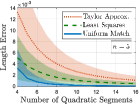
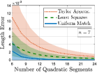
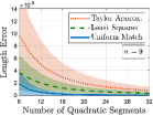
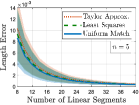
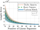
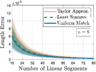
(a)	(b)	(c)	(d)	(e)	(f)

Figure 8: Normalized length error statistics of approximating $n^{\text{th}}$-order Bézier curves by (a, b, c) quadratic and (d, e, f) linear Bézier segments: (a, d) $n=5$, (b, e) $n=7$, (c, f) $n=9$, where the mean and the standard deviation of the error are presented by a line and a shaded region, respectively.

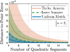
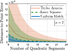
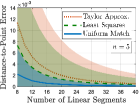
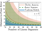
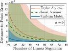
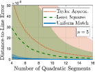
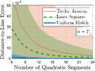
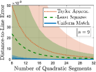
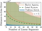
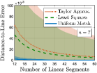
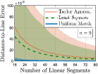
(a)	(b)	(c)	(d)	(e)	(f)

Figure 9: Normalized distance-to-point error statistics of approximating $n^{\text{th}}$-order Bézier curves by (a, b, c) quadratic and (d, e, f) linear Bézier segments: (a, d) $n=5$, (b, e) $n=7$, (c, f) $n=9$, where the mean and the standard deviation of the error are presented by a line and a shaded region, respectively.

(a)	(b)	(c)	(d)	(e)	(f)

Figure 10: Normalized distance-to-line error statistics of approximating $n^{\text{th}}$-order Bézier curves by (a, b, c) quadratic and (d, e, f) linear Bézier segments: (a, d) $n=5$, (b, e) $n=7$, (c, f) $n=9$, where the mean and the standard deviation of the error are presented by a line and a shaded region, respectively.

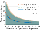
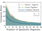
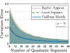
(a)	(b)	(c)

Figure 11: Normalized maximum curvature error statistics of quadratic approximations of Bézier curves for different number of segments: (a) $n=5$, (b) $n=7$, (c) $n=9$, where the mean and the standard deviation of the error are presented by a line and a shaded region, respectively. Note that for numerical stability we set an upper bound of $1000$ units on the maximum curvature, and any sample case with a larger maximum curvature is rejected.

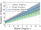
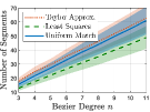
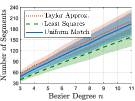
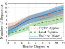
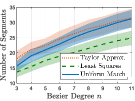
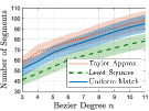
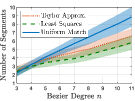
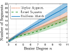
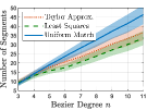
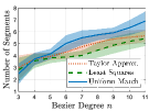
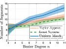
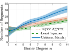
(a)	(b)	(c)	(d)	(e)	(f)

Figure 12: Relation between the number of segments and Bézier degree in adaptive Bézier approximation by (top) linear and (bottom) quadratic segments using (a, b, c) linear and (d, e, f) binary search. Here, the approximation tolerance is measured by the maximum control-point distance and set to be (a, d) 0.1, (b, e) 0.01, and (c, f) 0.001 units.

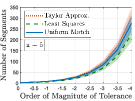
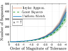
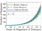
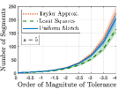
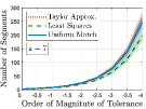
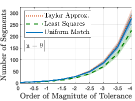
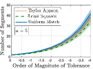
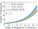
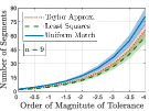
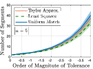
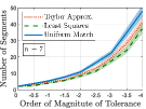
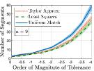
(a)	(b)	(c)	(d)	(e)	(f)

Figure 13: Relation between the number of segments and approximation tolerance in adaptive Bézier approximation by (top) linear and (bottom) quadratic segments using (a, b, c) linear and (d, e, f) binary search for Bézier order (a, d) $n=5$, (b, e) $n=7$, and (c, f) $n=9$. Here, the approximation tolerance is measured by the maximum control-point distance.

To determine approximation error statistics, we randomly generate Bézier control points that are uniformly distributed over the unit box $[0,1]\times[0,1]$. For the distance-to-point criterion, we select the origin as the point of interest; and for distance-to-line, we select the horizontal side of the unit box (i.e., the line segment joining the origin $(0,0)$ to point $(1,0)$). In Fig. 8-11, we provide sample statistics (mean and standard deviation) of normalized approximation errors of curve length, distance-to-point, distance-to-line, and maximum curvature versus the number of segments. It is visibly clear that the Bézier approximation with uniform matching reduction achieves significantly better performance in capturing curve length, distance-to-point and distance-to-line compared to the least squares and Taylor approximations. Especially, the end-point preservation property of uniform matching reduction plays a key role for its superior performance for the distance-to-point/line criteria presented in Fig. 9-10. We observe in Fig. 8 that Bézier approximations with linear segments have comparable accuracy for all three reduction methods, which can be explained by the limited representation power of linear curve segments. On the other hand, uniform matching reduction shows a superior performance for Bézier approximations with quadratic segments. Finally, as illustrated in Fig. 11, we see that all Bézier degree reduction methods perform equally well for approximating the maximum curvature of Bézier curves. This can be explained by the limited expresiveness of quadratic segments for approximating the first and second derivatives of Bézier curves since curvature is a function of the first and second curve derivatives.

VI-B Number of Segments vs. Bézier Degree and Tolerance

In this part, we numerically study how the number of segments automatically determined in adaptive Bézier approximation depends on the order of the Bézier curve and the approximation tolerance (specified in terms of the maximum control-point distance). We consider randomly generated Bézier control points over the unit box $[0,1]\times[0,1]$. To ensure scale invariance, we rescale Bézier control points to have a sample variance of unity. In Fig. 12 we present the average number of segments used in adaptive approximation of Bézier curves of different orders. For a fixed choice of an approximation tolerance, we observe that the number of segments grows linearly with the Bézier degree for linear search whereas the grow rate is sublinear for binary search. This is strongly aligned with the Bézier approximation rule proposed in Section V-B. Finally, as illustrated in Fig. 13, the average number of segments used in adaptive Bézier approximation grows exponentially with the negated order of magnitude of approximation tolerance $\varepsilon$, because the higher the accuracy the higher the spatial resolution.

VII Conclusion

In this paper, we introduce a novel adaptive Bézier approximation method that automatically splits and performs degree reduction on high-order Bézier curves to approximately represent them by multiple low-order Bézier segments at any given approximation tolerance measured by a Bézier metric. Accordingly, we propose a new maximum control-point distance for efficient and informative comparison of Bézier curves. We show that the maximum control-point distance defines a tight upper bound on standard Bézier metrics such as Hausdorff, parameterwise maximum, and Frobenious-norm distance of Bézier curves and can be used to geometrically bound Bézier curves with respect to each others. To better maintain the original curve shape, we also propose a new parameterwise matching reduction method that allows one to preserve a certain set of curve points (e.g., end points) after degree reduction. The matching reduction shows a superior approximation performance compared to standard least squares and Taylor approximations. Based on the explicit form of degree-one matching reduction error, we also suggest a rule of thumb for approximating $n^{\text{th}}$-order Bézier curves by $3(n-1)$ quadratic and $6(n-1)$ linear Bézier segments. Our extensive numerical studies demonstrates the effectiveness of the proposed methods and the validity of our Bezier approximation rule. Work now in progress targets applying these Bézier approximation tools in sensor-based reactive motion planning and trajectory optimization of nonholonomically constrained mobile robots and autonomous vehicles [54].

Appendix A Polynomial Basis Transformation Matrices

In this part, we provide the explicit formulas for the elements of polynomial basis transformation matrices.

Lemma 5 ([43])

(Monomial & Bernstein Basis Transformation) The transformation matrices between monomial and Bernstein basis vectors, i.e.,

$$\mathrm{m}_{n}(t) =\mathbf{T}_{\mathrm{b}}^{\mathrm{m}}(n)\mathrm{b}_{n}(t),$$ (83a)

$$\mathrm{b}_{n}(t) =\mathbf{T}_{\mathrm{m}}^{\mathrm{b}}(n)\mathrm{m}_{n}(t),$$ (83b)

are explicitly given by

$$\mathopen{}\mathclose{{}\left[\mathbf{T}_{\mathrm{m}}^{\mathrm{b}}(n)}\right]_{i+1,j+1} =\mathopen{}\mathclose{{}\left\{\begin{array}[]{r@{\,\,}l}(-1)^{(j-i)}\binom{n}{j}\binom{j}{i},&\text{ if }i\leq j\\ 0,&\text{ otherwise,}\end{array}}\right.$$ (84c)

$$\mathopen{}\mathclose{{}\left[\mathbf{T}_{\mathrm{b}}^{\mathrm{m}}(n)}\right]_{i+1,j+1} =\mathopen{}\mathclose{{}\left\{\begin{array}[]{r@{\,\,}l}\frac{\binom{j}{i}}{\binom{n}{i}},&\text{ if }i\leq j\\ 0,&\text{ otherwise,}\end{array}}\right.$$ (84f)

where $i,j\in\mathopen{}\mathclose{{}\left[0,1,\ldots,n}\right]$, and they are the inverse of each other

$$\mathbf{T}_{\mathrm{b}}^{\mathrm{m}}(n)^{-1}=\mathbf{T}_{\mathrm{m}}^{\mathrm{b}}(n).$$ (85)

Lemma 6

(Monomial-Taylor Basis Transformation) The transformation between monomial and Taylor bases, i.e.,

$$\mathrm{m}_{n}(t) =\mathbf{T}_{\mathrm{\tau}}^{\mathrm{m}}(n,t_{o})\mathrm{\tau}_{n,t_{o}}(t),$$ (86a)

$$\mathrm{\tau}_{n,t_{o}}(t) =\mathbf{T}_{\mathrm{m}}^{\mathrm{\tau}}(n,t_{o})\mathrm{m}_{n}(t),$$ (86b)

are explicitly given by

$$\mathopen{}\mathclose{{}\left[\mathbf{T}_{\mathrm{m}}^{\mathrm{\tau}}(n,t_{o})}\right]_{i+1,j+1} =\mathopen{}\mathclose{{}\left\{\begin{array}[]{@{}c@{\,\,}l}\binom{i}{j}(-t_{o})^{i-j}&\text{, if }i\geq j\\ 0&\text{, otherwise,}\end{array}}\right.$$ (87c)

$$\mathopen{}\mathclose{{}\left[\mathbf{T}_{\mathrm{\tau}}^{\mathrm{m}}(n,t_{o})}\right]_{i+1,j+1} =\mathopen{}\mathclose{{}\left\{\begin{array}[]{@{}c@{}l}\binom{i}{j}(t_{o})^{i-j}&\text{, if }i\geq j\\ 0&\text{, otherwise,}\end{array}}\right.$$ (87f)

where $i,j\in\{0,\ldots,n\}$, and they are the inverse of each other,

$$\mathbf{T}_{\mathrm{\tau}}^{\mathrm{m}}(n,t_{o})^{-1}=\mathbf{T}_{\mathrm{m}}^{\mathrm{\tau}}(n,t_{o}).$$ (88)

Proof.

See Appendix E-U. ∎

Accordingly, the transformation matrices between the Bernstein and Taylor bases, i.e.,

$$\mathrm{\tau}_{n,t_{o}}(t) =\mathbf{T}_{\mathrm{b}}^{\mathrm{\tau}}(n,t_{o})\mathrm{b}_{n}(t),$$ (89a)

$$\mathrm{b}_{n}(t) =\mathbf{T}_{\mathrm{\tau}}^{\mathrm{b}}(n,t_{o})\mathrm{\tau}_{n,t_{o}}(t),$$ (89b)

can be determined using the monomial basis as

$$\mathbf{T}_{\mathrm{b}}^{\mathrm{\tau}}(n,t_{o})=\mathbf{T}_{\mathrm{b}}^{\mathrm{m}}(n)\mathbf{T}_{\mathrm{m}}^{\mathrm{\tau}}(n,t_{o}),$$ (90a)

$$\mathbf{T}_{\mathrm{\tau}}^{\mathrm{b}}(n,t_{o})=\mathbf{T}_{\mathrm{\tau}}^{\mathrm{m}}(n,t_{o})\mathbf{T}_{\mathrm{m}}^{\mathrm{b}}(n),$$ (90b)

where $\mathbf{T}_{\mathrm{b}}^{\mathrm{\tau}}(n,t_{o})^{-1}=\mathbf{T}_{\mathrm{\tau}}^{\mathrm{b}}(n,t_{o})$.

Appendix B On Reparametrization of Polynomial Curves

In this part, we show how affine reparametrization of polynomial curves can be performed explicitly via Taylor basis.

Lemma 7

The Bernstein, monomial and Taylor basis vectors of degree $n$ (associated with a Taylor offset $t_{o}\in\mathbb{R}$) can be affinely reparametrized from interval $[a,b]$ to $[c,d]$ (with $a<b$ and $c<d$) as

$$\!\mathrm{b}_{n}(t) =\mathbf{T}_{\mathrm{\tau}}^{\mathrm{b}}(n,\widehat{t_{o}})\mathrm{diag}\mathopen{}\mathclose{{}\left(\!\mathrm{m}_{n}(\tfrac{b-a}{d-c})\!\!}\right)\mathbf{T}_{\mathrm{b}}^{\mathrm{\tau}}(n,t_{o})\mathrm{b}_{n}\!\mathopen{}\mathclose{{}\left(\!\tfrac{b-a}{d-c}t+\tfrac{ad-bc}{d-c}\!\!}\right),\!\!\!$$ (91a)

$$\!\mathrm{m}_{n}(t) =\mathbf{T}_{\mathrm{\tau}}^{\mathrm{m}}(n,\widehat{t_{o}})\mathrm{diag}\mathopen{}\mathclose{{}\left(\!\mathrm{m}_{n}(\tfrac{b-a}{d-c})\!\!}\right)\mathbf{T}_{\mathrm{m}}^{\mathrm{\tau}}(n,t_{o})\mathrm{m}_{n}\!\mathopen{}\mathclose{{}\left(\!\tfrac{b-a}{d-c}t+\tfrac{ad-bc}{d-c}\!\!}\right)\!,\!\!$$ (91b)

$$\!\mathrm{\tau}_{n,\widehat{t_{o}}}(t) =\mathrm{diag}\mathopen{}\mathclose{{}\left(\!\mathrm{m}_{n}(\tfrac{b-a}{d-c})\!\!}\right)\mathrm{\tau}_{n,t_{o}}\mathopen{}\mathclose{{}\left(\tfrac{b-a}{d-c}t+\tfrac{ad-bc}{d-c}\!}\right),$$ (91c)

where $\mathrm{diag}$ denotes the diagonal matrix with diagonal entries specified with its argument, and the reparametrized Taylor offset is given by the associated affine transformation as

$$\widehat{t_{o}}=\tfrac{d-c}{b-a}t_{a}-\tfrac{ad-bc}{b-a}.$$ (92)

Proof.

See Appendix E-V. ∎

Lemma 8

(Polynomial Curve Reparametrization) Bézier, monomial and Taylor curves of degree $n\in\mathbb{N}$ with respective control point matrices $\mathbf{P}_{n}=\mathopen{}\mathclose{{}\left[\mathrm{p}_{0},\ldots,\mathrm{p}_{n}}\right]$, $\mathbf{Q}_{n}=\mathopen{}\mathclose{{}\left[\mathrm{q}_{0},\ldots,\mathrm{q}_{n}}\right]$, and $\mathbf{Y}_{n}=\mathopen{}\mathclose{{}\left[\mathrm{y}_{0},\ldots,\mathrm{y}_{n}}\right]$ (and a Taylor offset $t_{o}\in\mathbb{R}$) can be affinely reparametrized from interval $[a,b]$ to $[c,d]$ (with $a<b$ and $c<d$) as

$$\mathrm{B}_{\widehat{\mathrm{p}}_{0},\ldots,\widehat{\mathrm{p}}_{n}}(t) =\mathrm{B}_{\mathrm{p}_{0},\ldots,\mathrm{p}_{n}}\mathopen{}\mathclose{{}\left(\tfrac{b-a}{d-c}t+\tfrac{ad-bc}{d-c}}\right),$$ (93a)

$$\mathrm{M}_{\widehat{\mathrm{q}}_{0},\ldots,\widehat{\mathrm{q}}_{n}}(t) =\mathrm{M}_{\mathrm{q}_{0},\ldots,\mathrm{q}_{n}}\mathopen{}\mathclose{{}\left(\tfrac{b-a}{d-c}t+\tfrac{ad-bc}{d-c}}\right),$$ (93b)

$$\Upsilon_{\widehat{\mathrm{y}}_{0},\ldots,\widehat{\mathrm{y}}_{n}}(t,\widehat{t_{o}}) =\Upsilon_{\mathrm{y}_{0},\ldots,\mathrm{y}_{n}}\mathopen{}\mathclose{{}\left(\tfrac{b-a}{d-c}t+\tfrac{ad-bc}{d-c},t_{o}}\right),$$ (93c)

with the corresponding reparametrized control point matrices $\widehat{\mathbf{P}}_{n}=\mathopen{}\mathclose{{}\left[\widehat{\mathrm{p}}_{0},\ldots,\widehat{\mathrm{p}}_{n}}\right]$, $\widehat{\mathbf{Q}}_{n}=\mathopen{}\mathclose{{}\left[\widehat{\mathrm{q}}_{0},\ldots,\widehat{\mathrm{q}}_{n}}\right]$, and $\widehat{\mathbf{Y}}_{n}=\mathopen{}\mathclose{{}\left[\widehat{\mathrm{y}}_{0},\ldots,\widehat{\mathrm{y}}_{n}}\right]$ that are given by

$$\widehat{\mathbf{P}}_{n} =\mathbf{P}_{n}\mathbf{T}_{\mathrm{\tau}}^{\mathrm{b}}(n,t_{o}\!)\mathrm{diag}\mathopen{}\mathclose{{}\left(\!\mathrm{m}_{n}(\tfrac{d-c}{b-a})\!}\right)\mathbf{T}_{\mathrm{b}}^{\mathrm{\tau}}(n,\widehat{t_{o}}),$$ (94a)

$$\widehat{\mathbf{Q}}_{n} =\mathbf{Q}_{n}\mathbf{T}_{\mathrm{\tau}}^{\mathrm{m}}(n,t_{o}\!)\mathrm{diag}\mathopen{}\mathclose{{}\left(\!\mathrm{m}_{n}(\tfrac{d-c}{b-a})\!}\right)\mathbf{T}_{\mathrm{m}}^{\mathrm{\tau}}(n,\widehat{t_{o}}),$$ (94b)

$$\widehat{\mathbf{Y}}_{n} =\mathbf{Y}_{n}\mathrm{diag}\mathopen{}\mathclose{{}\left(\mathrm{m}_{n}(\tfrac{d-c}{b-a})}\right),$$ (94c)

where $\widehat{t_{o}}=\tfrac{d-c}{b-a}t_{o}-\tfrac{ad-bc}{b-a}$.

Proof.

See Appendix E-W. ∎

Appendix C Matching Reduction in Monomial Basis

The matching reduction matrix can be explicitly computed using the monomial basis.

Lemma 9

(Matching Reduction in Monomial Basis) For any $n\geq m\in\mathbb{N}$ and distinct $t_{0},\ldots,t_{m}\in\mathbb{R}$, the parameterwise matching reduction matrix $\mathbf{R}_{t_{0},\ldots,t_{m}}(n,m)$ can be computed using monomial basis as

$$\mathbf{R}_{t_{0},\ldots,t_{m}}(n,m) =\mathbf{T}_{\mathrm{m}}^{\mathrm{b}}(n)\mathbf{m}_{n}(t_{0},\ldots,t_{m})\mathbf{m}_{m}(t_{0},\ldots,t_{m})^{-1}\mathbf{T}_{\mathrm{b}}^{\mathrm{m}}(m),$$

$$=\mathbf{T}_{\mathrm{m}}^{\mathrm{b}}(n)\mathopen{}\mathclose{{}\left[\begin{array}[]{@{}c@{}}\mathbf{I}_{(m+1)\times(m+1)}\\ \alpha_{1}(t_{0},\ldots,t_{m})\\ \vdots\\ \alpha_{n-m}(t_{0},\ldots,t_{m})\end{array}}\right]\mathbf{T}_{\mathrm{b}}^{\mathrm{m}}(m),$$ (99)

with row vectors $\alpha_{i}(t_{0},\ldots,t_{m})=[\alpha_{i,0},\ldots,\alpha_{i,m}]$ that are recursively defined as

$$\alpha_{i+1,k} =\alpha_{i,k-1}+\alpha_{i,m}\alpha_{1,k},$$ (100)

where base conditions of $\alpha_{i,-1}=0$ and $\alpha_{1,k}$ satisfying

$$t^{m+1}-\sum_{k=0}^{m}\alpha_{1,k}t^{k}=\prod_{k=0}^{m}(t-t_{k}).$$ (101)

Proof.

See Appendix LABEL:app.MatchingReductionMatrixMonomial. ∎

Appendix D Analytic Properties of Quadratic Bézier Curves

Motion planning with Bézier curves (around obstacles) requires determining critical geometric curve properties such as arc length, maximum absolute curvature, distance to a point or a line segment, and intersection with a halfspace. Fortunately, the low-degree of quadratic Bézier curves allows for simple analytic expressions of these curve properties enabling computationally efficient constrained motion planning, because quadratic bezier curves and derivatives have simple forms,

$$\mathrm{B}_{\mathrm{p}_{0},\mathrm{p}_{1},\mathrm{p}_{2}}(t) =(\mathrm{p}_{2}-2\mathrm{p}_{1}+\mathrm{p}_{0})t^{2}+2(\mathrm{p}_{1}-\mathrm{p}_{0})t+\mathrm{p}_{0},$$ (102a)

$$\mathrm{B}_{\mathrm{p}_{0},\mathrm{p}_{1},\mathrm{p}_{2}}^{\prime}(t) =2(\mathrm{p}_{1}-\mathrm{p}_{0})+2t(\mathrm{p}_{2}-2\mathrm{p}_{1}+\mathrm{p}_{0}),$$ (102b)

$$\mathrm{B}_{\mathrm{p}_{0},\mathrm{p}_{1},\mathrm{p}_{2}}^{\prime\prime}(t) =2(\mathrm{p}_{2}-2\mathrm{p}_{1}+\mathrm{p}_{0}).$$ (102c)

Proposition 19 ([55])

The arc length of a quadratic Bézier curve $\mathrm{B}_{\mathrm{p}_{0},\mathrm{p}_{1},\mathrm{p}_{2}}(t)$ over an interval $[t_{1},t_{2}]$ is given by

$$L(\mathrm{B}_{\mathrm{p}_{0},\mathrm{p}_{1},\mathrm{p}_{2}}([t_{1},t_{2}]))=2(I(t_{2})-I(t_{1}))$$ (103)

where $I(t)=\int R(t)\mathrm{d}t$ is the integral of $R(t)=\sqrt{at^{2}+bt+c}$ that is given for $a>0$ as [56]

$$I(t) =\frac{2at+b}{4a}R(t)+\frac{4ac-b^{2}}{8a\sqrt{a}}\ln|2\sqrt{a}R(t)+2at+b|$$ (104)

with

$$a =\|\mathrm{p}_{2}-2\mathrm{p}_{1}+\mathrm{p}_{0}\|^{2}$$ (105a)

$$b =2{(\mathrm{p}_{1}-\mathrm{p}_{0})}^{\mathrm{T}}(\mathrm{p}_{2}-2\mathrm{p}_{1}+\mathrm{p}_{0})$$ (105b)

$$c =\|\mathrm{p}_{1}-\mathrm{p}_{0}\|^{2}$$ (105c)

Otherwise (i.e., $a=0$), one has $I(t)=\sqrt{c}t=\|\mathrm{p}_{1}-\mathrm{p}_{0}\|t$.

Proof.

By definition, the arc length of a curve is given by the integral of the norm of its rate of change, i.e.,

$$L(\mathrm{B}_{\mathrm{p}_{0},\mathrm{p}_{1},\mathrm{p}_{2}}([t_{1},t_{2}])) =\int_{t_{1}}^{t_{2}}\|\mathrm{B}_{\mathrm{p}_{0},\mathrm{p}_{1},\mathrm{p}_{2}}^{\prime}(t)\|\mathrm{d}t$$ (106)

$$=\int_{t_{1}}^{t_{2}}2\|(\mathrm{p}_{1}-\mathrm{p}_{0})+t(\mathrm{p}_{2}-2\mathrm{p}_{1}+\mathrm{p}_{0})\|\mathrm{d}t\!\!$$ (107)

$$=2\int_{t_{1}}^{t_{2}}\sqrt{at^{2}+bt+c}\mathrm{d}t$$ (108)

where $a,b,c$ are defined as in (105). Also note that $a=0$ implies $b=0$, and so $\int\sqrt{at^{2}+bt+c}\mathrm{d}t=\sqrt{c}t$. Hence, the result follows. ∎

Proposition 20 ([57, 58])

The maximum absolute curvature of a planar quadratic Bézier curve $\mathrm{B}_{\mathrm{p}_{0},\mathrm{p}_{1},\mathrm{p}_{2}}(t)$, associated with $\mathrm{p}_{0},\mathrm{p}_{1},\mathrm{p}_{2}\in\mathbb{R}^{2}$, over an interval $[t_{1},t_{2}]$ satisfies

$$\max_{t\in[t_{1},t_{2}]}|\kappa(t)|=\mathopen{}\mathclose{{}\left\{\begin{array}[]{rl}|\kappa(t_{1})|&\text{, if }t_{\kappa}^{*}<t_{1}\\ |\kappa(t_{\kappa}^{*})|&\text{, if }t_{1}\leq t_{\kappa}^{*}\leq t_{2}\\ |\kappa(t_{2})|&\text{, if }t_{\kappa}^{*}>t_{2}\end{array}}\right.$$ (112)

where the quadratic Bézier curvature $\kappa(t)$ is given by

$$\kappa(t)=\frac{\det([\mathrm{p}_{1}-\mathrm{p}_{0},\mathrm{p}_{2}-\mathrm{p}_{1}])}{2\|(\mathrm{p}_{1}-\mathrm{p}_{0})(1-t)+(\mathrm{p}_{2}-\mathrm{p}_{1})t\|^{3}},$$ (113)

and the optimal curve parameter $t_{\kappa}^{*}$ and the maximum absolute curvature $|\kappa(t_{\kappa}^{*})|$ over $t\in\mathbb{R}$ are

$$t^{*}_{\kappa} =\operatornamewithlimits{argmax}\limits_{t\,\in\,\mathbb{R}}|\kappa(t)|=\frac{(\mathrm{p}_{0}-\mathrm{p}_{1})^{T}(\mathrm{p}_{2}-2\mathrm{p}_{1}+\mathrm{p}_{0})}{\|\mathrm{p}_{2}-2\mathrm{p}_{1}+\mathrm{p}_{0}\|^{2}},$$ (114)

$$|\kappa(t_{\kappa}^{*})| =\cfrac{\|\mathrm{p}_{2}-2\mathrm{p}_{1}+\mathrm{p}_{0}\|^{3}}{2\det([\mathrm{p}_{1}-\mathrm{p}_{0},\mathrm{p}_{2}-\mathrm{p}_{1}])^{2}}.$$ (115)

Proof.

The quadratic Bézier curvature can be determined as

$$\!\!\kappa(t) =\frac{\det\mathopen{}\mathclose{{}\left(\mathopen{}\mathclose{{}\left[\mathrm{B}_{\mathrm{p}_{0},\mathrm{p}_{1},\mathrm{p}_{2}}^{\prime}(t),\mathrm{B}_{\mathrm{p}_{0},\mathrm{p}_{1},\mathrm{p}_{2}}^{\prime\prime}(t)}\right]}\right)}{\|\mathrm{B}_{\mathrm{p}_{0},\mathrm{p}_{1},\mathrm{p}_{2}}^{\prime}(t)\|^{3}}$$ (116)

$$=\frac{\det{\mathopen{}\mathclose{{}\left[(\mathrm{p}_{1}-\mathrm{p}_{0})+t(\mathrm{p}_{2}-2\mathrm{p}_{1}+\mathrm{p}_{0}),(\mathrm{p}_{2}-2\mathrm{p}_{1}+\mathrm{p}_{0})}\right]}}{2\|(\mathrm{p}_{1}-\mathrm{p}_{0})+t(\mathrm{p}_{2}-2\mathrm{p}_{1}+\mathrm{p}_{0})\|^{3}}\!\!$$ (117)

$$=\frac{\det{\mathopen{}\mathclose{{}\left[(\mathrm{p}_{1}-\mathrm{p}_{0}),(\mathrm{p}_{2}-2\mathrm{p}_{1}+\mathrm{p}_{0})}\right]}}{2\|(\mathrm{p}_{1}-\mathrm{p}_{0})+t(\mathrm{p}_{2}-2\mathrm{p}_{1}+\mathrm{p}_{0})\|^{3}}$$

$$\hskip 28.45274pt+t\underbrace{\frac{\det{\mathopen{}\mathclose{{}\left[(\mathrm{p}_{2}-2\mathrm{p}_{1}+\mathrm{p}_{0}),(\mathrm{p}_{2}-2\mathrm{p}_{1}+\mathrm{p}_{0})}\right]}}{2\|(\mathrm{p}_{1}-\mathrm{p}_{0})+t(\mathrm{p}_{2}-2\mathrm{p}_{1}+\mathrm{p}_{0})\|^{3}}}_{=0}$$ (118)

$$=\frac{\det{\mathopen{}\mathclose{{}\left[(\mathrm{p}_{1}-\mathrm{p}_{0}),(\mathrm{p}_{2}-2\mathrm{p}_{1}+\mathrm{p}_{0})}\right]}}{2\|(\mathrm{p}_{1}-\mathrm{p}_{0})+t(\mathrm{p}_{2}-2\mathrm{p}_{1}+\mathrm{p}_{0})\|^{3}}$$ (119)

Hence, the maximum absolute curvature $|\kappa(t)|$ is achieved when $\|(\mathrm{p}_{1}-\mathrm{p}_{0})+t(\mathrm{p}_{2}-2\mathrm{p}_{1}+\mathrm{p}_{0})\|^{2}$ is minimized, which is a convex function of $t$ and its unique minimum can be determined by setting its derivative to zero as

$$0 =\frac{\mathrm{d}}{\mathrm{d}t}\|(\mathrm{p}_{1}-\mathrm{p}_{0})+t(\mathrm{p}_{2}-2\mathrm{p}_{1}+\mathrm{p}_{0})\|^{2}$$ (120)

$$=2{(\mathrm{p}_{2}-2\mathrm{p}_{1}+\mathrm{p}_{0})}^{\mathrm{T}}\mathopen{}\mathclose{{}\left((\mathrm{p}_{1}-\mathrm{p}_{0})+t(\mathrm{p}_{2}-2\mathrm{p}_{1}+\mathrm{p}_{0})}\right)$$ (121)

which corresponds to (114). Hence, due to the convexity of quadratic $\|(\mathrm{p}_{1}-\mathrm{p}_{0})+t(\mathrm{p}_{2}-2\mathrm{p}_{1}+\mathrm{p}_{0})\|^{2}$, the maximum absolute curvature is realized at $t_{\kappa}^{*}$ if $t_{\kappa}^{*}\in[t_{1},t_{2}]$; otherwise, the maximum value is at the closest boundary of the interval $[t_{1},t_{2}]$ to $t_{\kappa}^{*}$ as described in (112).

Finally, using the fact that $\det([\mathrm{a},\mathrm{b}])^{2}=\|\mathrm{a}\|^{2}\|\mathrm{b}\|^{2}-\mathopen{}\mathclose{{}\left({\mathrm{a}}^{\mathrm{T}}\mathrm{b}}\right)^{2}$ for any $\mathrm{a},\mathrm{b}\in\mathbb{R}^{2}$, one can verify that

$$|\kappa(t^{*}_{\kappa})| =\tfrac{|\det\mathopen{}\mathclose{{}\left(\mathopen{}\mathclose{{}\left[\mathrm{p}_{1}-\mathrm{p}_{0},\mathrm{p}_{2}-\mathrm{p}_{1}}\right]}\right)|\|\mathrm{p}_{2}-2\mathrm{p}_{1}+\mathrm{p}_{0}\|^{3}}{2\|(\mathrm{p}_{1}-\mathrm{p}_{0})\|\mathrm{p}_{2}-2\mathrm{p}_{1}+\mathrm{p}_{0}\|-\frac{{(\mathrm{p}_{0}-\mathrm{p}_{1})}^{\mathrm{T}}(\mathrm{p}_{2}-2\mathrm{p}_{1}+\mathrm{p}_{0})(\mathrm{p}_{2}-2\mathrm{p}_{1}+\mathrm{p}_{0})}{\|\mathrm{p}_{2}-2\mathrm{p}_{1}+\mathrm{p}_{0}\|}\|^{3}}$$ (122)

$$=\tfrac{|\det\mathopen{}\mathclose{{}\left(\mathopen{}\mathclose{{}\left[\mathrm{p}_{1}-\mathrm{p}_{0},\mathrm{p}_{2}-\mathrm{p}_{1}}\right]}\right)|\|\mathrm{p}_{2}-2\mathrm{p}_{1}+\mathrm{p}_{0}\|^{3}}{2\mathopen{}\mathclose{{}\left(\|\mathrm{p}_{1}-\mathrm{p}_{0}\|^{2}\|\mathrm{p}_{2}-2\mathrm{p}_{1}+\mathrm{p}_{0}\|^{2}-\mathopen{}\mathclose{{}\left({\mathrm{p}_{1}-\mathrm{p}_{0}}^{\mathrm{T}}(\mathrm{p}_{2}-2\mathrm{p}_{1}+\mathrm{p}_{0})}\right)^{2}}\right)^{\frac{3}{2}}}$$ (123)

$$=\tfrac{|\det\mathopen{}\mathclose{{}\left(\mathopen{}\mathclose{{}\left[\mathrm{p}_{1}-\mathrm{p}_{0},\mathrm{p}_{2}-\mathrm{p}_{1}}\right]}\right)|\|\mathrm{p}_{2}-2\mathrm{p}_{1}+\mathrm{p}_{0}\|^{3}}{2|\det\mathopen{}\mathclose{{}\left(\mathopen{}\mathclose{{}\left[\mathrm{p}_{1}-\mathrm{p}_{0},\mathrm{p}_{2}-\mathrm{p}_{1}}\right]}\right)|^{3}}$$ (124)

$$=\tfrac{\|\mathrm{p}_{2}-2\mathrm{p}_{1}+\mathrm{p}_{0}\|^{3}}{2\det\mathopen{}\mathclose{{}\left(\mathopen{}\mathclose{{}\left[\mathrm{p}_{1}-\mathrm{p}_{0},\mathrm{p}_{2}-\mathrm{p}_{1}}\right]}\right)^{2}}$$ (125)

which completes the proof. ∎

Proposition 21

The distance of a quadratic Bézier curve $\mathrm{B}_{\mathrm{p}_{0},\mathrm{p}_{1},\mathrm{p}_{2}}(t)$ to the origin over an interval $[t_{1},t_{2}]$ satisfies

$$\min_{t\in[t_{1},t_{2}]}\|\mathrm{B}_{\mathrm{p}_{0},\mathrm{p}_{1},\mathrm{p}_{2}}(t)\|=\min_{t\in T_{\mathrm{p}_{0},\mathrm{p}_{1},\mathrm{p}_{2}}}\|\mathrm{B}_{\mathrm{p}_{0},\mathrm{p}_{1},\mathrm{p}_{2}}(t)\|,$$ (126)

where the finite set of time instances is given by

$$T_{\mathrm{p}_{0},\mathrm{p}_{1},\mathrm{p}_{2}}([t_{1},t_{2}])=\mathopen{}\mathclose{{}\left\{t\in[t_{1},t_{2}]\,\Big{|}\,\sum\nolimits_{i=0}^{3}c_{i}t^{i}\!=\!0}\right\}\cup\mathopen{}\mathclose{{}\left\{t_{1},t_{2}}\right\},\!\!\!$$ (127)

with

$$c_{0} ={(\mathrm{p}_{1}-\mathrm{p}_{0})}^{\mathrm{T}}\mathrm{p}_{0},$$ (128a)

$$c_{1} ={(\mathrm{p}_{2}-2\mathrm{p}_{1}+\mathrm{p}_{0})}^{\mathrm{T}}\mathrm{p}_{0}+2\|\mathrm{p}_{1}-\mathrm{p}_{0}\|^{2},$$ (128b)

$$c_{2} =3{(\mathrm{p}_{2}-2\mathrm{p}_{1}+\mathrm{p}_{0})}^{\mathrm{T}}(\mathrm{p}_{1}-\mathrm{p}_{0}),$$ (128c)

$$c_{3} =\|\mathrm{p}_{2}-2\mathrm{p}_{1}+\mathrm{p}_{0}\|^{2}.$$ (128d)

Proof.

One can verify using (102) that the critical points of $\|\mathrm{B}_{\mathrm{p}_{0},\mathrm{p}_{1},\mathrm{p}_{2}}(t)\|$ over $\mathbb{R}$ satisfy the following cubic equation

$$0 ={\mathrm{B}_{\mathrm{p}_{0},\mathrm{p}_{1},\mathrm{p}_{2}}(t)}^{\mathrm{T}}\mathrm{B}_{\mathrm{p}_{0},\mathrm{p}_{1},\mathrm{p}_{2}}^{\prime}(t)=2(c_{3}t^{3}+c_{2}t^{2}+c_{1}t+c_{0})\!\!$$ (129)

where the coefficients $c_{0},c_{1},c_{2},c_{3}$ are defined as in (128). Hence, the quadratic bezier distance to the origin is realized in one of the critical points in $[t_{1},t_{2}]$ or on the boundary. ∎

Remark 1

The distance of a bezier curve $\mathrm{B}_{\mathrm{p}_{0},\ldots,\mathrm{p}_{n}}(t)$ to a point $\mathrm{q}\in\mathbb{R}^{d}$ or another bezier curve $\mathrm{B}_{\mathrm{q}_{0},\ldots,\mathrm{q}_{n}}(t)$ (with parameter-wise correspondence) can be formulated as its distance to the origin because

$$\mathrm{B}_{\mathrm{p}_{0},\ldots,\mathrm{p}_{n}}(t)-\mathrm{q} =\mathrm{B}_{\mathrm{p}_{0}-\mathrm{q},\ldots,\mathrm{p}_{n}-\mathrm{q}}(t)$$ (130)

$$\mathrm{B}_{\mathrm{p}_{0},\ldots,\mathrm{p}_{n}}(t)-\mathrm{B}_{\mathrm{q}_{0},\ldots,\mathrm{q}_{n}}(t) =\mathrm{B}_{\mathrm{p}_{0}-\mathrm{q}_{0},\ldots,\mathrm{p}_{n}-\mathrm{q}_{n}}(t)$$ (131)

Proposition 22

The distance of a quadratic Bézier curve $\mathrm{B}_{\mathrm{p}_{0},\mathrm{p}_{1},\mathrm{p}_{2}}(t)$ defined over the internal $[t_{1},t_{2}]$ to a linear Bézier curve $\mathrm{B}_{\mathrm{q}_{0},\mathrm{q}_{1}}(k)$ defined over the interval [$k_{1},k_{2}]$ can be analytically determined as

$$\min_{t\in[t_{1},t_{2}]}\min_{k\in[k_{1},k_{2}]}\|\mathrm{B}_{\mathrm{p}_{0},\mathrm{p}_{1},\mathrm{p}_{2}}(t)-\mathrm{B}_{\mathrm{q}_{0},\mathrm{q}_{1}}(k)\|$$

$$\hskip 71.13188pt=\min_{t\in\widehat{T}}\|\mathrm{B}_{\mathrm{p}_{0},\mathrm{p}_{1},\mathrm{p}_{2}}(t)-\mathrm{B}_{\mathrm{q}_{0},\mathrm{q}_{1}}(k^{*}(t))\|$$ (132)

using a finite set of critical time instances $\widehat{T}$ defined in terms of $T$ in (127) as

$$\widehat{T} =T_{\mathrm{p}_{0}-\mathrm{q}_{0},\mathrm{p}_{1}-\mathrm{q}_{0},\mathrm{p}_{2}-\mathrm{q}_{0}}([t_{1},t_{2}])$$

$$\hskip 56.9055pt\cup T_{\mathrm{p}_{0}-\mathrm{q}_{1},\mathrm{p}_{1}-\mathrm{q}_{1},\mathrm{p}_{2}-\mathrm{q}_{1}}([t_{1},t_{2}])$$

$$\hskip 113.81102pt\cup T_{\hat{\mathrm{p}}_{0},\hat{\mathrm{p}}_{1},\hat{\mathrm{p}}_{2}}([t_{1},t_{2}])$$ (133)

and the optimal line parameter $k^{*}(t)$ that is given by

$$k^{*}(t) =\min\mathopen{}\mathclose{{}\left(\max\mathopen{}\mathclose{{}\left(k_{1},\tfrac{{\mathopen{}\mathclose{{}\left(\mathrm{q}_{1}-\mathrm{q}_{0}}\right)}^{\mathrm{T}}}{\|\mathrm{q}_{1}-\mathrm{q}_{0}\|^{2}}\mathopen{}\mathclose{{}\left(\mathrm{B}_{\mathrm{p}_{0},\mathrm{p}_{1},\mathrm{p}_{2}}(t)-\mathrm{q}_{0}}\right)}\right),k_{2}}\right).\!\!$$ (134)

where

$$\hat{\mathrm{p}}_{i}=\mathopen{}\mathclose{{}\left(\mathbf{I}-\frac{(\mathrm{q}_{1}-\mathrm{q}_{0}){(\mathrm{q}_{1}-\mathrm{q}_{0})}^{\mathrm{T}}}{\|\mathrm{q}_{1}-\mathrm{q}_{0}\|^{2}}}\right)(\mathrm{p}_{i}-\mathrm{q}_{0}).$$ (135)

Proof.

Due to convexity, for any $t\in\mathbb{R}$, the line parameter

$$k(t)=\tfrac{{\mathopen{}\mathclose{{}\left(\mathrm{q}_{1}-\mathrm{q}_{0}}\right)}^{\mathrm{T}}}{\|\mathrm{q}_{1}-\mathrm{q}_{0}\|^{2}}\mathopen{}\mathclose{{}\left(\mathrm{B}_{\mathrm{p}_{0},\mathrm{p}_{1},\mathrm{p}_{2}}(t)-\mathrm{q}_{0}}\right)$$ (136)

minimizes $\|\mathrm{B}_{\mathrm{p}_{0},\mathrm{p}_{1},\mathrm{p}_{2}}(t)-\mathrm{B}_{\mathrm{q}_{0},\mathrm{q}_{1}}(k)\|$ over $\mathbb{R}$, i.e.,

$$0={(\mathrm{q}_{1}-\mathrm{q}_{0})}^{\mathrm{T}}\mathopen{}\mathclose{{}\left(\mathrm{B}_{\mathrm{p}_{0},\mathrm{p}_{1},\mathrm{p}_{2}}(t)-\mathrm{q}_{0}-k(t)(\mathrm{q}_{1}-\mathrm{q}_{0})}\right).$$ (137)

Hence, the optimal solution $k^{*}(t)$ over the interval $[k_{1},k_{2}]$ is given by (134) since the optimal solution of a quadratic optimization problem is realized at $k(t)$ if $k(t)\in[k_{1},k_{2}]$; otherwise, the optimum is at the closest interval boundary.

Similarly, the optimal bezier parameter is either related with a boundary point $\mathrm{q}_{0}$ and $\mathrm{q}_{1}$ of the line segment (corresponding to $T_{\mathrm{p}_{0}-\mathrm{q}_{0},\mathrm{p}_{1}-\mathrm{q}_{0},\mathrm{p}_{2}-\mathrm{q}_{0}}([t_{1},t_{2}])$ and $T_{\mathrm{p}_{0}-\mathrm{q}_{0},\mathrm{p}_{1}-\mathrm{q}_{0},\mathrm{p}_{2}-\mathrm{q}_{0}}([t_{1},t_{2}])$) or the minimum of $\|\mathrm{B}_{\mathrm{p}_{0},\mathrm{p}_{1},\mathrm{p}_{2}}(t)-\mathrm{B}_{\mathrm{q}_{0},\mathrm{q}_{1}}(k(t))\|$ where

$$\mathrm{B}_{\mathrm{q}_{0},\mathrm{q}_{1}}(k(t)) =\mathrm{q}_{0}+\tfrac{(\mathrm{q}_{1}-\mathrm{q}_{0}){(\mathrm{q}_{1}-\mathrm{q}_{0})}^{\mathrm{T}}}{\|\mathrm{q}_{1}-\mathrm{q}_{0}\|^{2}}(\mathrm{B}_{\mathrm{p}_{0},\mathrm{p}_{1},\mathrm{p}_{2}}(t)-\mathrm{q}_{0})$$ (138)

$$\mathrm{B}_{\mathrm{p}_{0},\mathrm{p}_{1},\mathrm{p}_{2}}(t)-\mathrm{B}_{\mathrm{q}_{0},\mathrm{q}_{1}}(k(t)) =\mathopen{}\mathclose{{}\left(\mathbf{I}-\tfrac{(\mathrm{q}_{1}-\mathrm{q}_{0}){(\mathrm{q}_{1}-\mathrm{q}_{0})}^{\mathrm{T}}}{\|\mathrm{q}_{1}-\mathrm{q}_{0}\|^{2}}}\right)(\mathrm{B}_{\mathrm{p}_{0},\mathrm{p}_{1},\mathrm{p}_{2}}(t)-\mathrm{q}_{0})$$ (139)

$$=\mathrm{B}_{\hat{\mathrm{p}}_{0},\hat{\mathrm{p}}_{1},\hat{\mathrm{p}}_{2}}(t)$$ (140)

which completes the proof. ∎

Proposition 23

The intersection of quadratic Bézier curve $\mathrm{B}_{\mathrm{p}_{0},\mathrm{p}_{1},\mathrm{p}_{2}}(t)$ defined over an interval $[t_{a},t_{b}]$ with a halfspace $H_{\mathrm{a},\mathrm{b}}=\mathopen{}\mathclose{{}\left\{\mathrm{x}\in\mathbb{R}^{d}|{\mathrm{a}}^{\mathrm{T}}(\mathrm{x}-\mathrm{b})\leq 0}\right\}$ satisfies

$$\mathopen{}\mathclose{{}\left\{t\in[t_{a},t_{b}]\big{|}{\mathrm{a}}^{\mathrm{T}}(\mathrm{B}_{\mathrm{p}_{0},\mathrm{p}_{1},\mathrm{p}_{2}}(t)-\mathrm{b})\geq 0}\right\}$$

$$\hskip 28.45274pt=\bigcup\mathopen{}\mathclose{{}\left\{[t_{i},t_{i+1}]|1\leq i<|T|,\mathrm{B}_{\mathrm{p}_{0},\mathrm{p}_{1},\mathrm{p}_{2}}(\frac{t_{i}+t_{i+1}}{2})\in H_{\mathrm{a},\mathrm{b}}}\right\}$$ (141)

where $(t_{1},t_{2},\ldots,t_{|T|})$ is the ascendingly ordered tuple of

$$T=\mathopen{}\mathclose{{}\left\{t\in[t_{a},t_{b}]\big{|}{\mathrm{a}}^{\mathrm{T}}(\mathrm{B}_{\mathrm{p}_{0},\mathrm{p}_{1},\mathrm{p}_{2}}(t)-\mathrm{b})=0}\right\}\cup\mathopen{}\mathclose{{}\left\{t_{a},t_{b}}\right\}$$ (142)

where ${\mathrm{a}}^{\mathrm{T}}(\mathrm{B}_{\mathrm{p}_{0},\mathrm{p}_{1},\mathrm{p}_{2}}(t)-\mathrm{b})=0$ is a quadratic equation.

Proof.

By definition, the roots of ${\mathrm{a}}^{\mathrm{T}}(\mathrm{B}_{\mathrm{p}_{0},\mathrm{p}_{1},\mathrm{p}_{2}}(t)-\mathrm{b})$ determines the Bezier parameters over $\mathbb{R}$ where the curve intersects the halfspace boundary. Hence, the ascendingly sorted elements of $T$ define a partition of the interval $[t_{a},t_{b}]$ whose consecutive pairs define the part of the bezier curve on the opposite sides of the halfspace. Therefore, the result follows. ∎

Appendix E Proofs

E-A Proof of Lemma 1

Proof.

The result follows from that $n^{\text{th}}$-order Bernstein polynomials, as well as monomials and Taylor polynomials of degree less than or equal to $n$, define a basis of $n+1$ linearly independent polynomials for $n^{\text{th}}$-order polynomials [43].

Alternatively, one can verify the result using polynomial basis transformations as follows. The monomial basis matrix $\mathbf{m}_{n}(t_{0},\ldots,t_{n})$, by definition, equals to the Vandermonde matrix, which is nonsingular for distinct $t_{0},\ldots,t_{n}$ [53]. The Bezier and Taylor basis matrices are also nonsingular due to the change of basis relation, i.e.,

$$\mathbf{b}_{n}(t_{0},\ldots,t_{n}) =\mathbf{T}_{\mathrm{m}}^{\mathrm{b}}(n)\mathbf{m}_{n}(t_{0},\ldots,t_{n}),$$ (143a)

$$\bm{\tau}_{n,t_{o}}(t_{0},\ldots,t_{n}) =\mathbf{T}_{\mathrm{\tau}}^{\mathrm{b}}(n,t_{o})\mathbf{m}_{n}(t_{0},\ldots,t_{n}),$$ (143b)

where $\mathbf{T}_{\mathrm{m}}^{\mathrm{b}}(n)$ and $\mathbf{T}_{\mathrm{\tau}}^{\mathrm{b}}(n,t_{o})$ are invertible triangular basis transformation matrices (see Lemmas 5 & 6). ∎

E-B Proof of Lemma 2

Proof.

Consider the basis transformation matrix $\mathbf{T}_{\mathrm{m}}^{\mathrm{b}}(n)$ from monomial to Bernstein basis. It follows by definition that

$$\mathbf{b}_{n}(t_{0},\ldots,t_{n})=\mathbf{T}_{\mathrm{m}}^{\mathrm{b}}(n)\mathbf{m}_{n}(t_{0},\ldots,t_{n}).$$ (144)

Since the monomial basis matrix $\mathbf{m}_{n}(t_{0},\ldots,t_{n})$ is invertible for any distinct $t_{0},\ldots,t_{n}\in\mathbb{R}$ (Lemma 1), we obtain

$$\mathbf{T}_{\mathrm{m}}^{\mathrm{b}}(n)=\mathbf{b}_{n}(t_{0},\ldots,t_{n})\mathbf{m}_{n}(t_{0},\ldots,t_{n})^{-1}.$$ (145)

Similarly, the result can be verified for any change of basis between Bernstein, Taylor and monomial bases, which completes the proof. ∎

E-C Proof of Lemma 3

Proof.

Let us focus on the equivalence of Bézier curves to monomial curves. The equivalence of Bézier and monomial curves means that for any distinct $t_{0},\ldots,t_{n}\in\mathbb{R}$ one has

$$\mathrm{B}_{\mathrm{p}_{0},\ldots,\mathrm{p}_{n}}(t_{0},\ldots,t_{n}) =\mathrm{M}_{\mathrm{p}_{0},\ldots,\mathrm{p}_{n}}(t_{0},\ldots,t_{n})$$ (146)

$$\mathbf{P}_{n}\mathbf{b}_{n}(t_{0},\ldots,t_{n}) =\mathbf{Q}_{n}\mathbf{m}_{n}(t_{0},\ldots,t_{n})$$ (147)

$$=\mathbf{Q}_{n}\mathbf{T}_{\mathrm{b}}^{\mathrm{m}}(n)\mathbf{b}_{n}(t_{0},\ldots,t_{n}).$$ (148)

Since the Bernstein basis matrix $\mathbf{b}_{n}(t_{0},\ldots,t_{n})$ is invertible for any distinct $t_{0},\ldots,t_{n}$ (Lemma 1), one can conclude that

$$\mathbf{P}_{n}=\mathbf{Q}_{n}\mathbf{T}_{\mathrm{b}}^{\mathrm{m}}(n)$$ (149)

which can be similarly extended for other polynomial curve equivalence relations. ∎

E-D Proof of Lemma 4

Proof.

For any $t_{0},\ldots,t_{n}\in\mathbb{R}$, by definition, affine Bezier reparametrization satisfies for $\widehat{t}_{i}=\tfrac{d-c}{b-a}t_{i}-\tfrac{ad-bc}{b-a}$ that

$$\widehat{\mathbf{P}}_{n}\mathbf{b}_{n}(\widehat{t}_{0},\ldots,\widehat{t}_{n})=\mathbf{P}_{n}\mathbf{b}_{n}(t_{0},\ldots,t_{n}).$$ (150)

Hence, we have the result since Bernstein basis matrices are invertible for any distinct parameters (Lemma 1), which also extends in a similar way to Taylor and monomial curves. ∎

E-E Proof of Proposition 1

Proof.

Using the following properties of Bernstein polynomials [44],

$$\int_{0}^{1}\!\!b_{i,n}(t)\mathrm{d}t=\scalebox{1.25}{$\frac{1}{n+1}$},\,\text{ and }\,b_{i,n}(t)b_{j,m}(t)=\frac{\binom{n}{i}\binom{n}{j}}{\binom{n+m}{i+j}}b_{i+j,n+m}(t)$$

one can verify the result as

$$\!\!d_{L2}(\mathrm{B}_{\mathrm{p}_{0},\ldots,\mathrm{p}_{n}},\mathrm{B}_{\mathrm{q}_{0},\ldots,\mathrm{q}_{n}})^{2} =\int_{0}^{1}\!\!\|\mathrm{B}_{\mathrm{p}_{0}-\mathrm{q}_{0},\ldots,\mathrm{p}_{n}-\mathrm{q}_{n}}(t)\|^{2}\mathrm{d}t,$$ (151)

$$=\sum_{i=0}^{n}\sum_{j=0}^{n}{\mathopen{}\mathclose{{}\left(\mathrm{p}_{i}-\mathrm{q}_{i}}\right)}^{\mathrm{T}}\mathopen{}\mathclose{{}\left(\mathrm{p}_{j}-\mathrm{q}_{j}}\right)\int_{0}^{1}\!\!b_{i,n}(t)b_{j,n}(t)\mathrm{d}t,$$ (152)

$$=\sum_{i=0}^{n}\sum_{j=0}^{n}{\mathopen{}\mathclose{{}\left(\mathrm{p}_{i}-\mathrm{q}_{i}}\right)}^{\mathrm{T}}\mathopen{}\mathclose{{}\left(\mathrm{p}_{j}-\mathrm{q}_{j}}\right)\frac{\binom{n}{i}\binom{n}{j}}{\binom{2n}{i+j}}\int_{0}^{1}\!\!b_{i+j,2n}(t)\mathrm{d}t,\!\!\!$$ (153)

$$=\sum_{i=0}^{n}\sum_{j=0}^{n}\frac{1}{2n+1}\frac{\binom{n}{i}\binom{n}{j}}{\binom{2n}{i+j}}{\mathopen{}\mathclose{{}\left(\mathrm{p}_{i}-\mathrm{q}_{i}}\right)}^{\mathrm{T}}\mathopen{}\mathclose{{}\left(\mathrm{p}_{j}-\mathrm{q}_{j}}\right),$$ (154)

$$=\mathrm{tr}\mathopen{}\mathclose{{}\left((\mathbf{P}_{n}-\mathbf{Q}_{n})\mathbf{W}_{n}{(\mathbf{P}_{n}-\mathbf{Q}_{n})}^{\mathrm{T}}}\right),$$ (155)

which completes the proof. ∎

E-F Proof of Proposition 2

Proof.

By Definition 5, the Bézier parameterwise-maximum distance defines an upper bound on the Bézier Haussdoff distance, i.e.,

$$d_{H}(\mathrm{B}_{\mathrm{p}_{0},\ldots,\mathrm{p}_{n}},\mathrm{B}_{\mathrm{q}_{0},\ldots,\mathrm{q}_{n}}) \leq d_{M}(\mathrm{B}_{\mathrm{p}_{0},\ldots,\mathrm{p}_{n}},\mathrm{B}_{\mathrm{q}_{0},\ldots,\mathrm{q}_{n}}).$$ (156)

Similarly, the equivalence relation of the Frobenius distance and the control-point distances is evident from Definition 4 and Definition 6 as

$$d_{C}(\mathrm{B}_{\mathrm{p}_{0},\ldots,\mathrm{p}_{n}},\mathrm{B}_{\mathrm{q}_{0},\ldots,\mathrm{q}_{n}}) \hskip 56.9055pt=\max_{i=0,\ldots,n}\|\mathrm{p}_{i}-\mathrm{q}_{i}\|,$$ (157)

$$\leq d_{F}(\mathrm{B}_{\mathrm{p}_{0},\ldots,\mathrm{p}_{n}},\mathrm{B}_{\mathrm{q}_{0},\ldots,\mathrm{q}_{n}})=\sqrt{\sum\nolimits_{i=0}^{n}\|\mathrm{p}_{i}-\mathrm{q}_{i}\|^{2}},\!\!\!$$ (158)

$$\leq\sqrt{n}d_{C}(\mathrm{B}_{\mathrm{p}_{0},\ldots,\mathrm{p}_{n}},\mathrm{B}_{\mathrm{q}_{0},\ldots,\mathrm{q}_{n}}).$$ (159)

Hence, the result follows from Jensen’s equality for the squared Euclidean distance because

$$\|\mathrm{B}_{\mathrm{p}_{0},\ldots,\mathrm{p}_{n}}(t)-\mathrm{B}_{\mathrm{q}_{0},\ldots,\mathrm{q}_{n}}(t)\|^{2} =\|\mathrm{B}_{\mathrm{p}_{0}-\mathrm{q}_{0},\ldots,\mathrm{p}_{n}-\mathrm{q}_{n}}(t)\|^{2},$$ (160)

$$=\|\sum_{i=0}^{n}b_{i,n}(t)(\mathrm{p}_{i}-\mathrm{q}_{i})\|^{2}\leq\sum_{i=0}^{n}b_{i,n}(t)\|\mathrm{p}_{i}-\mathrm{q}_{i}\|^{2},$$ (161)

$$\leq\max_{i}\|\mathrm{p}_{i}-\mathrm{q}_{i}\|^{2}.$$ (162)

Note that the Bernstein polynomials sum to one over $t\in[0,1]$, i.e., $\sum_{i=0}^{n}b_{i,n}(t)=1$ for all $t\in[0,1]$ (Property 3). ∎

E-G Proof of Proposition 3

Proof.

The ordering relation of Bézier metrics in Proposition 2 and the convexity of Bézier curves in Property 3 imply that

$$\min_{t^{\prime}\in[0,1]}\!\|\mathrm{B}_{\mathrm{p}_{0},\ldots,\mathrm{p}_{n}}(t)-\mathrm{B}_{\mathrm{q}_{0},\ldots,\mathrm{q}_{n}}(t^{\prime})\|\leq\|\mathrm{B}_{\mathrm{p}_{0},\ldots,\mathrm{p}_{n}}(t)-\mathrm{B}_{\mathrm{q}_{0},\ldots,\mathrm{q}_{n}}(t)\|,$$

$$\hskip 14.22636pt\leq d_{M}(\mathrm{B}_{\mathrm{p}_{0},\ldots,\mathrm{p}_{n}},\mathrm{B}_{\mathrm{q}_{0},\ldots,\mathrm{q}_{n}})\leq d_{C}(\mathrm{B}_{\mathrm{p}_{0},\ldots,\mathrm{p}_{n}},\mathrm{B}_{\mathrm{q}_{0},\ldots,\mathrm{q}_{n}}),\!\!\!$$ (163)

and so the result follows. ∎

E-H Proof of Proposition 4

Proof.

The sufficiency of elevated control points in (48) can be verified as

$$\mathrm{B}_{\mathrm{q}_{0},\ldots,\mathrm{q}_{m}}(t) =\mathbf{Q}_{m}\mathrm{b}_{m}(t)$$ (164a)

$$=\mathbf{P}_{n}\mathbf{E}(n,m)\mathrm{b}_{m}(t),$$ (164b)

$$=\mathbf{P}_{n}\mathbf{T}_{\mathrm{m}}^{\mathrm{b}}(n)\mathbf{I}_{(n+1)\times(m+1)}\mathbf{T}_{\mathrm{b}}^{\mathrm{m}}(m)\mathrm{b}_{m}(t),\!\!\!$$ (164c)

$$=\mathbf{P}_{n}\mathbf{T}_{\mathrm{m}}^{\mathrm{b}}(n)\mathbf{I}_{(n+1)\times(m+1)}\mathrm{m}_{m}(t),\!\!\!$$ (164d)

$$=\mathbf{P}_{n}\mathbf{T}_{\mathrm{m}}^{\mathrm{b}}(n)\mathrm{m}_{n}(t),$$ (164e)

$$=\mathbf{P}_{n}\mathrm{b}_{n}(t)=\mathrm{B}_{\mathrm{p}_{0},\ldots,\mathrm{p}_{n}}(t).$$ (164f)

To show the necessity of parameterwise coincidence, consider distinct parameters $t_{0},\ldots,t_{m}\in\mathbb{R}$ with $t_{i}\neq t_{j}$ for all $i\neq j$. Since square Bernstein basis matrices of distinct parameters are invertible (Lemma 1), using the coinciding curve points at $t_{0},\ldots,t_{m}$, i.e.,

$$\mathbf{P}_{n}\mathbf{b}_{n}(t_{0},\ldots,t_{m})=\mathbf{Q}_{m}\mathbf{b}_{m}(t_{0},\ldots,t_{m}),$$ (165)

one can obtain an explicit expression for $\mathbf{E}(n,m)$ as

$$\mathbf{Q}_{m} =\mathbf{P}_{n}\mathbf{b}_{n}(t_{0},\ldots,t_{m})\mathbf{b}_{m}(t_{0},\ldots,t_{m})^{-1},\!\!\!$$ (166)

$$=\mathbf{P}_{n}\mathbf{E}(n,m),$$ (167)

which can be further simplified using the Bernstein-to-monomial basis transformation as

$$\mathbf{E}(n,m) \hskip 5.69054pt=\mathbf{b}_{n}(t_{0},\ldots,t_{m})\mathbf{b}_{m}(t_{0},\ldots,t_{m})^{-1},$$ (168)

$$=\mathbf{T}_{\mathrm{m}}^{\mathrm{b}}(n)\mathbf{m}_{n}(t_{0},\ldots,t_{m})\mathbf{m}_{m}(t_{0},\ldots,t_{m})^{-1}\mathbf{T}_{\mathrm{b}}^{\mathrm{m}}(m),\!\!\!$$ (169)

$$=\mathbf{T}_{\mathrm{m}}^{\mathrm{b}}(n)\mathbf{I}_{(n+1)\times(m+1)}\mathbf{T}_{\mathrm{b}}^{\mathrm{m}}(m),$$ (170)

which completes the proof. ∎

E-I Proof of Proposition 5

Proof.

By definition in (49), we have

$$\mathbf{E}(n,m)\mathrm{b}_{m}(t) =\mathbf{T}_{\mathrm{m}}^{\mathrm{b}}(n)\mathbf{I}_{(n+1)\times(m+1)}\mathbf{T}_{\mathrm{b}}^{\mathrm{m}}(m)\mathrm{b}_{m}(t)$$ (171)

$$=\mathbf{T}_{\mathrm{m}}^{\mathrm{b}}(n)\mathbf{I}_{(n+1)\times(m+1)}\mathrm{m}_{m}(t)$$ (172)

$$=\mathbf{T}_{\mathrm{m}}^{\mathrm{b}}(n)\mathrm{m}_{n}(t)=\mathrm{b}_{n}(t).$$ (173)

Therefore, the result follows since the Bernstein basis matrix $\mathbf{b}_{m}(t_{0},\ldots,t_{m})$ is invertible (Lemma 1). ∎

E-J Proof of Proposition 6

Proof.

We below provide a proof by induction.

$\bullet$ Base Case: ($n\leq m\leq n+1$): If $m=n$, then one trivially has $\mathbf{E}(n,n)=\mathbf{I}_{(n+1)\times(n+1)}$. If $m=n+1$, then

$$\mathopen{}\mathclose{{}\left[\mathbf{E}(n,n+1)}\right]_{i+1,j+1}=\mathopen{}\mathclose{{}\left\{\begin{array}[]{@{}c@{\,}l@{}}1-\frac{j}{n+1}&\text{, if }j=i,\\ \frac{j}{n+1}&\text{, if }j=i+1,\\ 0&\text{, otherwise,}\end{array}}\right.$$ (177)

which follows from (50) and the following degree-one elevation property of Bernstein polynomials [43]

$$b_{i,n}(t)=\mathopen{}\mathclose{{}\left(1-\tfrac{i}{n+1}}\right)b_{i,n+1}(t)+\tfrac{i+1}{n+1}b_{i+1,n+1}(t).$$ (178)

Also note that $\binom{n}{j}/\binom{n+1}{j}=1-\frac{j}{n+1}$ and $\binom{n}{j-1}/\binom{n+1}{j}=\frac{j}{n+1}$. Hence, the result holds for the base case.

$\bullet$ Induction Step ($m>n+1$): Suppose the results holds for $\mathbf{E}(n,m-1)$, then one can determine $\mathbf{E}(n,m)$ as

$$\mathbf{E}(n,m)=\mathbf{E}(n,m-1)\mathbf{E}(m-1,m),$$ (179)

because the degree elevation operation preserves the original Bézier curve exactly. Hence, it follows from (177) that

$$\mathopen{}\mathclose{{}\left[\mathbf{E}(n,m)}\right]_{i+1,j+1}\! =\!\sum_{k=0}^{m}\!\mathopen{}\mathclose{{}\left[\mathbf{E}(n,m-1)}\right]_{i+1,k+1}\mathopen{}\mathclose{{}\left[\mathbf{E}(m-1,m)}\right]_{k+1,j+1},\!\!\!\!\!$$ (180)

$$=\mathopen{}\mathclose{{}\left[\mathbf{E}(n,m-1)}\right]_{i+1,j}\mathopen{}\mathclose{{}\left[\mathbf{E}(m-1,m)}\right]_{j,j+1}$$

$$+\mathopen{}\mathclose{{}\left[\mathbf{E}(n,m-1)}\right]_{i+1,j+1}\mathopen{}\mathclose{{}\left[\mathbf{E}(m-1,m)}\right]_{j+1,j+1},\!\!$$ (181)

$$=\tfrac{j}{m}\mathopen{}\mathclose{{}\left[\mathbf{E}(n,m-1)}\right]_{i+1,j}+\mathopen{}\mathclose{{}\left(1-\tfrac{j}{m}}\right)\mathopen{}\mathclose{{}\left[\mathbf{E}(n,m-1)}\right]_{i+1,j+1}.\!\!\!$$ (182)

Note that $\mathopen{}\mathclose{{}\left[\mathbf{E}(n,m-1)}\right]_{i+1,j+1}\neq 0$ iff $0\leq j-i\leq m-n-1$; and $\mathopen{}\mathclose{{}\left[\mathbf{E}(n,m-1)}\right]_{i+1,j}\neq 0$ iff $1\leq j-i\leq m-n$. Hence, we complete the induction step by checking the following cases:

$\circ$ If $j-i>m-n$ or $j-i<0$, then $\mathopen{}\mathclose{{}\left[\mathbf{E}(n,m-1)}\right]_{i+1,j+1}=0$ and $\mathopen{}\mathclose{{}\left[\mathbf{E}(n,m-1)}\right]_{i+1,j}=0$, and so

$$\mathopen{}\mathclose{{}\left[\mathbf{E}(n,m)}\right]_{i+1,j+1}=0.$$ (183)

$\circ$ If $j-i=m-n$, then $\mathopen{}\mathclose{{}\left[\mathbf{E}(n,m-1)}\right]_{i+1,j+1}=0$ and so

$$\mathopen{}\mathclose{{}\left[\mathbf{E}(n,m)}\right]_{i+1,j+1}=\tfrac{j}{m}\mathopen{}\mathclose{{}\left[\mathbf{E}(n,m-1)}\right]_{i+1,j}=\tfrac{j}{m}\frac{\binom{n}{i}}{\binom{m-1}{j-1}}=\frac{\binom{n}{i}}{\binom{m}{j}}.$$ (184)

$\circ$ If $j-i=0$, then $\mathopen{}\mathclose{{}\left[\mathbf{E}(n,m-1)}\right]_{i+1,j}=0$ and so

$$\mathopen{}\mathclose{{}\left[\mathbf{E}(n,m)}\right]_{i+1,j+1} =\mathopen{}\mathclose{{}\left(1-\tfrac{j}{m}}\right)\mathopen{}\mathclose{{}\left[\mathbf{E}(n,m-1)}\right]_{i+1,j+1},$$ (185)

$$=\mathopen{}\mathclose{{}\left(1-\tfrac{j}{m}}\right)\frac{\binom{n}{i}}{\binom{m-1}{j}}=\frac{\binom{n}{i}}{\binom{m}{j}}.$$ (186)

$\circ$ Otherwise (i.e., $0<j-i<m-n$), we have

$$\mathopen{}\mathclose{{}\left[\mathbf{E}(n,m)}\right]_{i+1,j+1} =\tfrac{j}{m}\mathopen{}\mathclose{{}\left[\mathbf{E}(n,m-1)}\right]_{i+1,j}$$

$$\hskip 22.76219pt+\mathopen{}\mathclose{{}\left(1-\tfrac{j}{m}}\right)\mathopen{}\mathclose{{}\left[\mathbf{E}(n,m-1)}\right]_{i+1,j+1},\!\!$$ (187)

$$=\tfrac{j}{m}\frac{\binom{n}{i}\binom{m-n-1}{j-i-1}}{\binom{m-1}{j-1}}+\mathopen{}\mathclose{{}\left(1-\tfrac{j}{m}}\right)\frac{\binom{n}{i}\binom{m-n-1}{j-i}}{\binom{m-1}{j}},$$ (188)

$$=\frac{\binom{n}{i}\binom{m-n-1}{j-i-1}}{\frac{m}{j}\binom{m-1}{j-1}}+\frac{\binom{n}{i}\binom{m-n-1}{j-i}}{\frac{m}{m-j}\binom{m-1}{j}},$$ (189)

$$=\frac{\binom{n}{i}}{\binom{m}{j}}\mathopen{}\mathclose{{}\left(\!\binom{m-n-1}{j-i-1}+\binom{m-n-1}{j-i}\!}\right),$$ (190)

$$=\frac{\binom{n}{i}\binom{m-n}{j-i}}{\binom{m}{j}},$$ (191)

which completes the proof. ∎

E-K Proof of Proposition 7

Proof.

The result can be verified using either (49) or (51) with the fact that if a square matrix $\mathbf{B}$ is full rank (i.e., invertible), then $\mathrm{rank}(\mathbf{A}\mathbf{B})=\mathrm{rank}(\mathbf{A})$ for any matrix $\mathbf{A}$ that is conformable for the multiplication $\mathbf{A}\mathbf{B}$ [60]. ∎

E-L Proof of Proposition 8

Proof.

The column-sum property of the elevation matrix follows from Proposition 5,

$$\mathbf{E}(n,m) =\mathbf{b}_{n}(t_{0},\ldots,t_{m})\mathbf{b}_{m}(t_{0},\ldots,t_{m})^{-1},$$ (192)

and the convexity of Bernstein polynomials (Property 3),

$$\mathbf{1}_{1\times(n+1)}\mathbf{b}_{n}(t_{0},\ldots,t_{m}) =\mathbf{1}_{1\times(m+1)},$$ (193)

$$\mathbf{1}_{1\times(m+1)}\mathbf{b}_{m}(t_{0},\ldots,t_{m}) =\mathbf{1}_{1\times(m+1)}\mathbf{b}_{m}(t_{0},\ldots,t_{m})^{-1},$$ (194)

$$=\mathbf{1}_{1\times(m+1)},$$ (195)

where $t_{0},\ldots,t_{m}\in\mathbb{R}$ are any distinct reals.

The row-sum property of the elevation matrix can be proven by induction as follows.

$\bullet$ Base Case ($n\leq m\leq n+1)$: If $m=n$, then one has $\mathbf{E}(n,n)=\mathbf{I}_{(n+1)\times(n+1)}$ and so the result holds. For $m=n+1$,

$$\mathopen{}\mathclose{{}\left[\mathbf{E}(n,n+1)}\right]_{i+1,j+1}=\mathopen{}\mathclose{{}\left\{\begin{array}[]{@{}c@{\,\,}l@{}}1-\frac{i}{n+1}&\text{, if }j=i,\\ \frac{i+1}{n+1}&\text{, if }j=i+1,\\ 0&\text{, otherwise}.\end{array}}\right.$$ (199)

Hence, the row sum of $\mathbf{E}(n,n+1)$ is $\frac{n+2}{n+1}$, i.e.,

$$\sum_{j=0}^{n+1}\mathopen{}\mathclose{{}\left[\mathbf{E}(n,n+1)}\right]_{i+1,j+1}=1-\tfrac{i}{n+1}+\tfrac{i+1}{n+1}=\tfrac{n+2}{n+1}.$$ (200)

$\bullet$ Induction ($m>n+1$). Suppose that the result holds for $\mathbf{E}(n,m-1)$. Hence, using $\mathbf{E}(n,m)=\mathbf{E}(n,m-1)\mathbf{E}(m-1,m)$, one can conclude that the row sum of multiplication of two matrices is the multiplication of the their row sums, i.e.,

$$\sum_{j=0}^{m}\mathopen{}\mathclose{{}\left[\mathbf{E}(n,m)}\right]_{i+1,j+1}\!\!$$

$$=\!\!\sum_{j=0}^{m}\sum_{k=0}^{m-1}\!\mathopen{}\mathclose{{}\left[\mathbf{E}(n,m-1)}\right]_{i+1,k+1}\mathopen{}\mathclose{{}\left[\mathbf{E}(m-1,m)}\right]_{k+1,j+1},\!\!$$ (201)

$$=\mathopen{}\mathclose{{}\left(\sum_{k=0}^{m-1}\mathopen{}\mathclose{{}\left[\mathbf{E}(n,m-1)}\right]_{i+1,k+1}\!\!}\right)\!\!\mathopen{}\mathclose{{}\left(\sum_{j=0}^{m}\mathopen{}\mathclose{{}\left[\mathbf{E}(m-1,m)}\right]_{k+1,j+1}\!\!}\right),\!\!$$ (202)

$$=\frac{m}{n+1}\frac{m+1}{m}=\frac{m+1}{n+1},$$ (203)

which completes the proof. ∎

E-M Proof of Proposition 9

Proof.

The result directly follows from Definition 3 of the L2-norm distance because degree elevation exactly represents Bézier curves with more control points (Definition 7). ∎

E-N Proof of Proposition 10

Proof.

Using the column- and row-sum property of the elevation matrix in Proposition 8, one can obtain the result by applying Jensen’s inequality as

$$d_{F}(\mathrm{B}_{[\mathrm{p}_{0},\ldots,\mathrm{p}_{n}]\mathbf{E}(n,m)},\mathrm{B}_{[\mathrm{q}_{0},\ldots,\mathrm{q}_{n}]\mathbf{E}(n,m)})$$

$$=\|(\mathbf{P}_{n}-\mathbf{Q}_{n})\mathbf{E}(n,m)\|_{F}^{2},$$ (204)

$$=\sum_{j=0}^{m}\|(\mathbf{P}_{n}-\mathbf{Q}_{n})\mathbf{E}(n,m)_{j+1}\|^{2},$$ (205)

$$\leq\sum_{j=0}^{m}\sum_{i=0}^{n}[\mathbf{E}(n,m)]_{i+1,j+1}\|\mathrm{p}_{i}-\mathrm{q}_{i}\|^{2},$$ (206)

$$=\sum_{i=0}^{n}\|\mathrm{p}_{i}-\mathrm{q}_{i}\|^{2}\sum_{j=0}^{m}[\mathbf{E}(n,m)]_{i+1,j+1},\!\!$$ (207)

$$=\tfrac{m+1}{n+1}d_{F}(\mathrm{B}_{\mathrm{p}_{0},\ldots,\mathrm{p}_{n}},\mathrm{B}_{\mathrm{q}_{0},\ldots,\mathrm{q}_{n}})^{2},$$ (208)

where $\mathbf{E}(n,m)_{j+1}$ denotes the $(j+1)^{\text{th}}$-column of $\mathbf{E}(n,m)$. ∎

E-O Proof of Proposition 11

Proof.

Let $\mathbf{E}(n,m)=\mathopen{}\mathclose{{}\left[\mathrm{e}_{0},\ldots,\mathrm{e}_{m}}\right]$. Then, the result can be verified using Jensen’s inequality and the unit column sum property of the elevation matrix (Proposition 8) as follows:

$$d_{C}(\mathrm{B}_{\mathopen{}\mathclose{{}\left[\mathrm{p}_{0},\ldots,\mathrm{p}_{n}}\right]\mathbf{E}(n,m)},\mathrm{B}_{\mathopen{}\mathclose{{}\left[\mathrm{q}_{0},\ldots,\mathrm{q}_{n}}\right]\mathbf{E}(n,m)}) =\max_{i=0\ldots m}\!\|(\mathbf{P}-\mathbf{Q})\mathrm{e}_{i}\|,\!\!\!$$ (209)

$$\leq\max_{j=0,\ldots,n}\|\mathrm{p}_{j}-\mathrm{q}_{j}\|=d_{C}(\mathrm{B}_{\mathrm{p}_{0},\ldots,\mathrm{p}_{n}},\mathrm{B}_{\mathrm{q}_{0},\ldots,\mathrm{q}_{n}}),$$ (210)

where the Jensen’s inequality and ${\mathbf{1}}^{\mathrm{T}}\mathrm{e}_{i}=1$ imply that

$$\|(\mathbf{P}-\mathbf{Q})\mathrm{e}_{i}\|\leq\max_{j=0,\ldots,n}\|\mathrm{p}_{j}-\mathrm{q}_{j}\|$$ (211)

and this completes the proof. ∎

E-P Proof of Proposition 13

Proof.

Using the following matrix identities [61]

$$\frac{\partial}{\partial\mathbf{X}}\mathrm{tr}\mathopen{}\mathclose{{}\left(\mathbf{X}\mathbf{A}}\right) ={\mathbf{A}}^{\mathrm{T}},\quad\text{ and }\quad\frac{\partial}{\partial\mathbf{X}}\mathrm{tr}\mathopen{}\mathclose{{}\left(\mathbf{X}\mathbf{A}{\mathbf{X}}^{\mathrm{T}}}\right)=\mathbf{X}(\mathbf{A}+{\mathbf{A}}^{\mathrm{T}}),$$ (212)

and the explicit form of the L2-norm distance in Proposition 1, one can verify the optimality of the least squares reduction with respect to the L2-norm distance as follows

$$\frac{\partial}{\partial\mathbf{Q}_{m}}d_{L2}(\mathrm{B}_{\mathrm{p}_{0},\ldots,\mathrm{p}_{n}},\mathrm{B}_{\mathopen{}\mathclose{{}\left[\mathrm{q}_{0},\ldots,\mathrm{q}_{m}}\right]\mathbf{E}(m,n)})^{2}$$

$$\hskip 14.22636pt=\frac{\partial}{\partial\mathbf{Q}_{m}}\mathrm{tr}\mathopen{}\mathclose{{}\left(\!\!(\mathbf{P}_{n}-\mathbf{Q}_{m}\mathbf{E}(m,n))\mathbf{W}_{n}{(\mathbf{P}_{n}-\mathbf{Q}_{m}\mathbf{E}(m,n))\!}^{\mathrm{T}}\!}\right),\!\!\!\!$$ (213)

$$\hskip 14.22636pt=2(\mathbf{Q}_{m}\mathbf{E}(m,n)-\mathbf{P}_{n})\mathbf{W}_{n},$$ (214)

which equals to zero for $\mathbf{Q}_{m}=\mathbf{P}_{n}\mathbf{R}(n,m)$. Thus, the global optimality follows from the convexity of the squared L2-norm distance.

Similarly, due to its strong relation with linear least squares, the Frobenius-norm distance of Bézier curves

$$d_{F}(\mathrm{B}_{\mathrm{p}_{0},\ldots,\mathrm{p}_{n}},\mathrm{B}_{[\mathrm{q}_{0},\ldots,\mathrm{q}_{m}]\mathbf{E}(m,n)})=\|\mathbf{P}_{n}-\mathbf{Q}_{m}\mathbf{E}(m,n)\|_{F},$$ (215)

is minimized via the pseudo-inverse $\mathbf{E}(m,n)^{+}$ of $\mathbf{E}(m,n)$ at

$$\mathbf{Q}_{m}=\mathbf{P}_{n}\mathbf{E}(m,n)^{+}=\mathbf{P}_{n}\mathbf{R}_{L2}(n,m),$$ (216)

which completes the proof. ∎

E-Q Proof of Proposition 14

Proof.

The result can be verified using (49) and (64) as

$$\mathbf{E}(m,n)\mathbf{R}_{\mathrm{\tau},t_{o}}(n,m)$$

$$=\mathbf{T}_{\mathrm{m}}^{\mathrm{b}}(m)\mathbf{I}_{(m+1)\times(n+1)}\mathbf{T}_{\mathrm{b}}^{\mathrm{m}}(n)\mathbf{T}_{\mathrm{\tau}}^{\mathrm{b}}(n,t_{o})\mathbf{I}_{(n+1)\times(m+1)}\mathbf{T}_{\mathrm{b}}^{\mathrm{\tau}}(m,t_{o}),\!\!\!\!$$ (217)

$$=\mathbf{T}_{\mathrm{m}}^{\mathrm{b}}(m)\underbrace{\mathbf{I}_{m\times n}\mathbf{T}_{\mathrm{\tau}}^{\mathrm{m}}(n,t_{o})\mathbf{I}_{n\times m}}_{=\mathbf{T}_{\mathrm{\tau}}^{\mathrm{m}}(m,t_{o})}\mathbf{T}_{\mathrm{b}}^{\mathrm{\tau}}(m,t_{o}),$$ (218)

$$=\mathbf{T}_{\mathrm{m}}^{\mathrm{b}}(m)\mathbf{T}_{\mathrm{\tau}}^{\mathrm{m}}(m,t_{o})\mathbf{T}_{\mathrm{b}}^{\mathrm{\tau}}(m,t_{o}),$$ (219)

$$=\mathbf{T}_{\mathrm{m}}^{\mathrm{b}}(m)\mathbf{T}_{\mathrm{b}}^{\mathrm{m}}(m)=\mathbf{I}_{(m+1)\times(m+1)}.$$ (220)

which completes the proof. ∎

E-R Proof of Proposition 15

Proof.

Since $\mathbf{b}(t_{0},\ldots,t_{m})^{-1}\mathbf{b}_{m}(t_{0},\ldots,t_{m})=\mathbf{I}_{(m+1)\times(m+1)}$, we have for any $t_{i}\in\mathopen{}\mathclose{{}\left\{t_{0},\ldots,t_{m}}\right\}$ that

$$\mathrm{B}_{\mathrm{q}_{0},\ldots,\mathrm{q}_{m}}(t_{i}) \hskip 34.1433pt=[\mathrm{q}_{0},\ldots,\mathrm{q}_{m}]\mathrm{b}_{m}(t_{i}),$$ (221a)

$$=[\mathrm{p}_{0},\ldots,\mathrm{p}_{n}]\mathbf{R}_{t_{0},\ldots,t_{m}}(n,m)\mathrm{b}_{m}(t_{i}),$$ (221b)

$$=[\mathrm{p}_{0},\ldots,\mathrm{p}_{n}]\mathbf{b}_{n}(t_{0},\ldots,t_{m})\mathbf{b}_{m}(t_{0},\ldots,t_{m})^{-1}\mathrm{b}_{m}(t_{i}),\!\!\!$$ (221c)

$$=[\mathrm{p}_{0},\ldots,\mathrm{p}_{n}]\mathrm{b}_{n}(t_{i})=\mathrm{B}_{\mathrm{p}_{0},\ldots,\mathrm{p}_{n}}(t_{i}).$$ (221d)

Thus, the matching reduction preserves the curve at $t_{i}$. ∎

E-S Proof of Proposition 16

Proof.

Consider some additional distinct parameters $t_{m+1},\ldots,t_{n}\in\mathbb{R}$ that are different from $t_{0},\ldots,t_{m}$. Then the result can be verified using Proposition 5 as

$$\!\mathbf{E}(m,n)\mathbf{R}_{t_{0},\ldots,t_{m}}(n,m) =\mathbf{E}(m,n)\mathbf{b}_{n}(t_{0},\ldots,t_{m})\mathbf{b}_{m}(t_{0},\ldots,t_{m})^{-1}\!\!\!,\!\!\!\!$$ (222)

$$=\mathbf{b}_{m}(t_{0},\ldots,t_{m})\mathbf{b}_{m}(t_{0},\ldots,t_{m})^{-1},$$ (223)

$$=\mathbf{I}_{(m+1)\times(m+1)},$$ (224)

which completes the proof. ∎

E-T Proof of Proposition 18

Proof.

The matching reduction matrix $\mathbf{R}_{t_{0},\ldots,t_{n}}(n+1,n)$ can be expressed in the monomial basis using the basis transformation between Bernstein and monomial bases as

$$\mathbf{R}_{t_{0},\ldots,t_{n}}(n+1,n) =\mathbf{b}_{n+1}(t_{0},\ldots,t_{n})\mathbf{b}_{n}(t_{0},\ldots,t_{n})^{-1},$$ (225)

$$=\mathbf{T}_{\mathrm{m}}^{\mathrm{b}}(n+1)\mathbf{m}_{n+1}(t_{0},\ldots,t_{n})\mathbf{m}_{n}(t_{0},\ldots,t_{n})^{-1}\mathbf{T}_{\mathrm{b}}^{\mathrm{m}}(n),$$ (226)

$$=\mathbf{T}_{\mathrm{m}}^{\mathrm{b}}(n+1)\mathopen{}\mathclose{{}\left[\begin{array}[]{c}\mathbf{I}_{(n+1)\times(n+1)}\\ \mathopen{}\mathclose{{}\left[t_{0}^{n+1},\ldots,t_{n}^{n+1}}\right]\mathbf{m}_{n}(t_{0},\ldots,t_{n})^{-1}\end{array}}\right]\mathbf{T}_{\mathrm{b}}^{\mathrm{m}}(n).\!\!\!$$ (229)

Hence, the degree-one matching reduction difference can be written for $\mathbf{Q}_{n}=[\mathrm{q}_{0},\ldots,\mathrm{q}_{n}]$ and $\mathbf{P}_{n+1}=[\mathrm{p}_{0},\ldots,\mathrm{p}_{n+1}]$ as

$$\mathrm{B}_{\mathrm{p}_{0},\ldots,\mathrm{p}_{n+1}}(t)-\mathrm{B}_{\mathrm{q}_{0},\ldots,\mathrm{q}_{n}}(t)=\mathbf{P}_{n+1}\mathrm{b}_{n+1}(t)-\mathbf{Q}_{n}\mathrm{b}_{n}(t),$$ (230)

$$\hskip 5.69054pt=\mathbf{P}_{n+1}\mathbf{T}_{\mathrm{m}}^{\mathrm{b}}(n+1)\mathrm{m}_{n+1}(t)$$

$$\hskip 14.22636pt-\mathbf{P}_{n+1}\mathbf{T}_{\mathrm{m}}^{\mathrm{b}}(n+1)\mathopen{}\mathclose{{}\left[\begin{array}[]{@{}c@{}}\mathbf{I}_{(n+1)\times(n+1)}\\ \mathopen{}\mathclose{{}\left[t_{0}^{n+1},\ldots,t_{n}^{n+1}}\right]\mathbf{m}_{n}(t_{0},\ldots,t_{n})^{-1}\end{array}}\right]\mathbf{T}_{\mathrm{b}}^{\mathrm{m}}(n)\mathrm{b}_{n}(t),\!\!\!$$ (233)

$$\hskip 5.69054pt=\mathbf{P}_{n+1}\mathbf{T}_{\mathrm{m}}^{\mathrm{b}}(n+1)\!\mathopen{}\mathclose{{}\left(\!\!\mathrm{m}_{n+1}(t)\!-\!\mathopen{}\mathclose{{}\left[\begin{array}[]{@{}c@{}}\mathbf{I}_{(n+1)\times(n+1)}\!\!\!\!\\ \mathopen{}\mathclose{{}\left[t_{0}^{n+1},\ldots,t_{n}^{n+1}}\right]\mathbf{m}_{n}(t_{0},\ldots,t_{n})^{-1}\!\end{array}}\right]\mathrm{m}_{n}(t)\!\!\!}\right),\!\!\!$$ (236)

$$\hskip 5.69054pt=\mathbf{P}_{n+1}\mathbf{T}_{\mathrm{m}}^{\mathrm{b}}(n+1)\!\!\mathopen{}\mathclose{{}\left[\begin{array}[]{@{}c@{}}0\\ \vdots\\ 0\\ 1\end{array}}\right]\!\!\mathopen{}\mathclose{{}\left(t^{n+1}\!-[t_{0}^{n+1},\ldots,t_{n}^{n+1}]\mathbf{m}_{n}(t_{0},\ldots,t_{n})^{-1}\mathrm{m}_{n}(t)\!}\right).\!\!\!$$ (241)

Now observe that for any distinct $t_{0},\ldots,t_{n}\in\mathbb{R}$ one has

$$t^{n+1}-[t_{0}^{n+1},\ldots,t_{n}^{n+1}]\mathbf{m}_{n}(t_{0},\ldots,t_{n})^{-1}\mathrm{m}_{n}(t)=\prod_{i=0}^{n}(t-t_{i}),$$ (242)

which is zero at $t=t_{0},\ldots,t_{n}$. We also have from Lemma 5

$$\mathopen{}\mathclose{{}\left[\mathbf{T}_{\mathrm{m}}^{\mathrm{b}}(n+1)}\right]_{i+1,n+2} =(-1)^{n+1-i}\binom{n+1}{n+1}\binom{n+1}{i},$$ (243)

$$=(-1)^{n+1-i}\binom{n+1}{i}.$$ (244)

Hence, the matching reduction difference is given by

$$\mathrm{B}_{\mathrm{p}_{0},\ldots,\mathrm{p}_{n+1}}(t)-\mathrm{B}_{\mathrm{q}_{0},\ldots,\mathrm{q}_{n}}(t)\!=\!\mathopen{}\mathclose{{}\left(\sum_{i=0}^{n+1}\!(-1)^{n+1-i}\binom{n+1}{i}\mathrm{p}_{i}\!\!}\right)\!\!\prod_{i=0}^{n}(t-t_{i}),$$ (245)

which completes the proof. ∎

E-U Proof of Lemma 6

Proof.

The monomial-to-Taylor basis transformation $\mathbf{T}_{\mathrm{m}}^{\mathrm{\tau}}$ directly follows from the binomial formula,

$$(t-t_{o})^{i}=\sum_{j=0}^{i}\tbinom{i}{j}(-t_{o})^{i-j}t^{j}.$$ (246)

Similarly, the Taylor-to-monomial basis transformation $\mathbf{T}_{\mathrm{m}}^{\mathrm{\tau}}$ can be obtained using the binomial formula as

$$t^{i}=(t-t_{o}+t_{o})^{i}=\sum_{j=0}^{i}\binom{i}{j}t_{o}^{i-j}(t-t_{o})^{j}.$$ (247)

Finally, the monomial-to-Taylor and Taylor-to-monomial transformations are inverses of each other since they are lower triangular matrices with all ones in the main diagonal (i.e., $\det\mathopen{}\mathclose{{}\left(\mathbf{T}_{\mathrm{m}}^{\mathrm{\tau}}(n,t_{o})}\right)=\det\mathopen{}\mathclose{{}\left(\mathbf{T}_{\mathrm{\tau}}^{\mathrm{m}}(n,t_{o})}\right)=1$), and

$$\mathrm{m}_{n}(t)=\mathbf{T}_{\mathrm{\tau}}^{\mathrm{m}}(n,t_{o})\mathrm{\tau}_{n,t_{o}}(t)=\mathbf{T}_{\mathrm{\tau}}^{\mathrm{m}}(n,t_{o})\mathbf{T}_{\mathrm{m}}^{\mathrm{\tau}}(n,t_{o})\mathrm{m}_{n}(t)$$ (248)

$$\mathrm{\tau}_{n,t_{o}}(t)=\mathbf{T}_{\mathrm{m}}^{\mathrm{\tau}}(n,t_{o})\mathrm{m}_{n}(t)=\mathbf{T}_{\mathrm{m}}^{\mathrm{\tau}}(n,t_{o})\mathbf{T}_{\mathrm{\tau}}^{\mathrm{m}}(n,t_{o})\mathrm{\tau}_{n,t_{o}}(t)$$ (249)

hold for all $t\in\mathbb{R}$. ∎

E-V Proof of Lemma 7

Proof.

For Taylor basis reparametrization, the result follows from the definition of monomial and Taylor basis because

$$\mathopen{}\mathclose{{}\left(\tfrac{b-a}{d-c}t+\tfrac{ad-bc}{d-c}-t_{o}}\right)^{k} =\mathopen{}\mathclose{{}\left(\tfrac{b-a}{d-c}}\right)^{k}\mathopen{}\mathclose{{}\left(t-\tfrac{d-c}{b-a}t_{o}+\tfrac{ad-bc}{b-a}}\right)^{k}$$ (250)

$$=\mathopen{}\mathclose{{}\left(\tfrac{b-a}{d-c}}\right)^{k}\mathopen{}\mathclose{{}\left(t-\widehat{t_{o}}}\right)^{k}$$ (251)

For Bernstein basis reparametrization, the results can be verified using the change of basis between Bernstein and Taylor bases as

$$\mathrm{b}_{n}(t) \hskip 11.38109pt=\mathbf{T}_{\mathrm{\tau}}^{\mathrm{b}}(n,\widehat{t_{o}})\mathrm{\tau}_{n,\widehat{t_{o}}}(t)$$ (252)

$$=\mathbf{T}_{\mathrm{\tau}}^{\mathrm{b}}(n,\widehat{t_{o}})\mathrm{diag}\mathopen{}\mathclose{{}\left(\mathrm{m}_{n}(\tfrac{b-a}{d-c})}\right)\mathrm{\tau}_{n,t_{o}}\mathopen{}\mathclose{{}\left(\tfrac{b-a}{d-c}t+\tfrac{ad-bc}{d-c}}\right)$$ (253)

$$=\mathbf{T}_{\mathrm{\tau}}^{\mathrm{b}}(n,\widehat{t_{o}})\mathrm{diag}\mathopen{}\mathclose{{}\left(\mathrm{m}_{n}(\tfrac{b-a}{d-c})}\right)\mathbf{T}_{\mathrm{b}}^{\mathrm{\tau}}(n,t_{o})\mathrm{b}_{n}\mathopen{}\mathclose{{}\left(\tfrac{b-a}{d-c}t+\tfrac{ad-bc}{d-c}}\right)\!\!\!$$ (254)

which also extends to the monomial basis reparametrization in a similar way and so completes the proof. ∎

E-W Proof of Lemma 8

Proof.

For Bézier curve reparametrization, the result follows from the Bernstein basis reparametrization in Lemma 7 as

$$\mathrm{B}_{\mathrm{p}_{0},\ldots,\mathrm{p}_{n}}\mathopen{}\mathclose{{}\left(\tfrac{b-a}{d-c}t+\tfrac{ad-bc}{d-c}}\right) =\mathbf{P}_{n}\mathrm{b}_{n}\mathopen{}\mathclose{{}\left(\tfrac{b-a}{d-c}t+\tfrac{ad-bc}{d-c}}\right)$$ (255)

$$=\mathbf{P}_{n}\mathbf{T}_{\mathrm{\tau}}^{\mathrm{b}}(n,t_{o})\mathrm{diag}\mathopen{}\mathclose{{}\left(\mathrm{m}_{n}(\tfrac{d-c}{b-a})}\right)\mathbf{T}_{\mathrm{b}}^{\mathrm{\tau}}(n,\widehat{t_{o}})\mathrm{b}_{n}\mathopen{}\mathclose{{}\left(t}\right)$$ (256)

$$=\widehat{\mathbf{P}}_{n}\mathrm{b}_{n}\mathopen{}\mathclose{{}\left(t}\right)$$ (257)

which similarly extends to the monomial and Taylor curve reparametrization as well. ∎

E-X Proof of Lemma 9

Proof.

It follow from the Bernstein-to-monomial basis transformation that

$$\mathbf{R}_{t_{0},\ldots,t_{m}}(n,m) =\mathbf{b}_{n}(t_{0},\ldots,t_{m})\mathbf{b}_{m}(t_{0},\ldots,t_{m})^{-1},$$ (258)

$$=\mathbf{T}_{\mathrm{m}}^{\mathrm{b}}(n)\mathbf{m}_{n}(t_{0},\ldots,t_{m})\mathbf{m}_{m}(t_{0},\ldots,t_{m})^{-1}\mathbf{T}_{\mathrm{b}}^{\mathrm{m}}(m),$$ (259)

$$=\mathbf{T}_{\mathrm{m}}^{\mathrm{b}}(n)\mathopen{}\mathclose{{}\left[\begin{array}[]{@{}c@{}}\mathbf{I}_{(m+1)\times(m+1)}\\ \mathopen{}\mathclose{{}\left[t_{0}^{m+1},\ldots,t_{m}^{m+1}}\right]\mathbf{m}_{m}(t_{0},\ldots,t_{m})^{-1}\\ \vdots\\ \mathopen{}\mathclose{{}\left[t_{0}^{n},\ldots,t_{m}^{n}}\right]\mathbf{m}_{m}(t_{0},\ldots,t_{m})^{-1}\end{array}}\right]\mathbf{T}_{\mathrm{b}}^{\mathrm{m}}(m).\!\!\!$$ (264)

To complete the proof, we show below that the rows of the middle matrix following the identity matrix satisfy the recursion in (100) with the base case of (101). Hence, we first consider the base case where

$$[\alpha_{1,0},\ldots,\alpha_{1,m}]=\mathopen{}\mathclose{{}\left[t_{0}^{m+1},\ldots,t_{m}^{m+1}}\right]\mathrm{m}_{m}(t_{0},\ldots,t_{m})^{-1},$$ (265)

$$\mathopen{}\mathclose{{}\left[t_{0}^{m+1},\ldots,t_{m}^{m+1}}\right]=[\alpha_{1,0},\ldots,\alpha_{1,m}]\mathrm{m}_{m}(t_{0},\ldots,t_{m}),$$ (266)

which can be equivalently written as

$$t^{m+1}-\sum_{k=0}^{m}\alpha_{1,k}t^{k}=0\quad\forall t=t_{0},\ldots,t_{m}.$$ (267)

Since parameters $t_{0},\ldots,t_{m}$ are distinct, $\prod_{k=0}^{m}(t-t_{k})$ is the unique polynomial of order $m+1$ whose roots are $t_{0},\ldots,t_{m}$ with the unity coefficient of the monomial $t^{m+1}$. Therefore, we obtain the base case in (101) as

$$t^{m+1}-\sum_{k=0}^{m}\alpha_{1,k}t^{k}=\prod_{k=0}^{m}(t-t_{k}).$$ (268)

Now consider the $(m+i+1)^{\text{th}}$-row,

$$[\alpha_{i+1,0},\ldots,\alpha_{i+1,m}] =\mathopen{}\mathclose{{}\left[t_{0}^{m+i+1},\ldots,t_{m}^{m+i+1}}\right]\mathbf{m}_{m}(t_{0},\ldots,t_{m})^{-1},$$ (269)

$$\mathopen{}\mathclose{{}\left[t_{0}^{m+i+1},\ldots,t_{m}^{m+i+1}}\right] =[\alpha_{i+1,0},\ldots,\alpha_{i+1,m}]\mathbf{m}_{m}(t_{0},\ldots,t_{m}),\!\!\!$$ (270)

which is equivalent to

$$\sum_{k=0}^{m}\alpha_{i+1,k}t^{k} =t^{m+i+1}=t^{m+i}t,$$ (271)

$$=t\sum_{k=0}^{m}\alpha_{i,k}t^{k}=\alpha_{i,m}t^{m+1}+\sum_{k=0}^{m-1}\alpha_{i,k}t^{k+1},$$ (272)

$$=\sum_{k=0}^{m}(\alpha_{i,m}\alpha_{1,k}+\alpha_{i,k-1})t^{k},$$ (273)

where $\alpha_{i,-1}=0$. This implies the recursion relation in (100) and so the result follows. ∎

References

- [1] D. Mellinger and V. Kumar, “Minimum snap trajectory generation and control for quadrotors,” in IEEE International Conference on Robotics and Automation (ICRA), 2011, pp. 2520–2525.
- [2] C. Richter, A. Bry, and N. Roy, “Polynomial trajectory planning for aggressive quadrotor flight in dense indoor environments,” Robotics Research, Springer Tracts in Advanced Robotics, pp. 649–666, 2016.
- [3] W. Ding, W. Gao, K. Wang, and S. Shen, “An efficient B-spline-based kinodynamic replanning framework for quadrotors,” IEEE Transactions on Robotics, vol. 35, no. 6, pp. 1287–1306, 2019.
- [4] F. Gao, W. Wu, Y. Lin, and S. Shen, “Online safe trajectory generation for quadrotors using fast marching method and Bernstein basis polynomial,” in IEEE Int. Conf. Robot. Autom., 2018, pp. 344–351.
- [5] J. Tordesillas, B. T. Lopez, M. Everett, and J. P. How, “Faster: Fast and safe trajectory planner for navigation in unknown environments,” IEEE Transactions on Robotics, pp. 1–17, 2021.
- [6] D. González, J. Pérez, V. Milanés, and F. Nashashibi, “A review of motion planning techniques for automated vehicles,” IEEE Trans. Intell. Transp. Syst., vol. 17, no. 4, pp. 1135–1145, 2016.
- [7] W. Ding, L. Zhang, J. Chen, and S. Shen, “Safe trajectory generation for complex urban environments using spatio-temporal semantic corridor,” IEEE Robot. Autom. Lett., vol. 4, no. 3, pp. 2997–3004, 2019.
- [8] X. Qian, I. Navarro, A. de La Fortelle, and F. Moutarde, “Motion planning for urban autonomous driving using Bézier curves and MPC,” in IEEE Inter. Conf. Intell. Transp. Syst., 2016, pp. 826–833.
- [9] J. Pérez, J. Godoy, J. Villagrá, and E. Onieva, “Trajectory generator for autonomous vehicles in urban environments,” in IEEE International Conference on Robotics and Automation (ICRA), 2013, pp. 409–414.
- [10] H. Ozaki and C.-J. Lin, “Optimal B-spline joint trajectory generation for collision-free movements of a manipulator under dynamic constraints,” in IEEE Int. Conf. Robot. Autom., 1996, pp. 3592–3597.
- [11] K. Hauser and V. Ng-Thow-Hing, “Fast smoothing of manipulator trajectories using optimal bounded-acceleration shortcuts,” in IEEE Int. Conf. Robot. Autom., 2010, pp. 2493–2498.
- [12] C. Scheiderer, T. Thun, and T. Meisen, “Bézier curve based continuous and smooth motion planning for self-learning industrial robots,” Procedia Manufacturing, vol. 38, pp. 423–430, 2019.
- [13] X. Zhao, Z. Cao, W. Geng, Y. Yu, M. Tan, and X. Chen, “Path planning of manipulator based on RRT-connect and Bézier curve,” in IEEE International Conference on CYBER Technology in Automation, Control, and Intelligent Systems (CYBER), 2019, pp. 649–653.
- [14] A. Ravankar, A. A. Ravankar, Y. Kobayashi, Y. Hoshino, and C.-C. Peng, “Path smoothing techniques in robot navigation: State-of-the-art, current and future challenges,” Sensors, vol. 18, no. 9, 2018.
- [15] S. M. LaValle, Planning Algorithms. Cambridge University Press, 2006.
- [16] M. J. Van Nieuwstadt and R. M. Murray, “Real-time trajectory generation for differentially flat systems,” International Journal of Robust and Nonlinear Control, vol. 8, no. 11, pp. 995–1020, 1998.
- [17] A. Bry, C. Richter, A. Bachrach, and N. Roy, “Aggressive flight of fixed-wing and quadrotor aircraft in dense indoor environments,” Int. J. Robot. Res., vol. 34, no. 7, pp. 969–1002, 2015.
- [18] S. Liu, M. Watterson, K. Mohta, K. Sun, S. Bhattacharya, C. J. Taylor, and V. Kumar, “Planning dynamically feasible trajectories for quadrotors using safe flight corridors in 3-d complex environments,” IEEE Robotics and Automation Letters, vol. 2, no. 3, pp. 1688–1695, 2017.
- [19] W. Hönig, J. A. Preiss, T. K. S. Kumar, G. S. Sukhatme, and N. Ayanian, “Trajectory planning for quadrotor swarms,” IEEE Transactions on Robotics, vol. 34, no. 4, pp. 856–869, 2018.
- [20] J.-w. Choi, R. E. Curry, and G. H. Elkaim, “Continuous curvature path generation based on Bézier curves for autonomous vehicles,” IAENG Int. Journal of Applied Mathematics, vol. 40, no. 2, pp. 91–101, 2010.
- [21] D. González, J. Pérez, R. Lattarulo, V. Milanés, and F. Nashashibi, “Continuous curvature planning with obstacle avoidance capabilities in urban scenarios,” in IEEE International Conference on Intelligent Transportation Systems (ITSC), 2014, pp. 1430–1435.
- [22] S. Tang and V. Kumar, “Safe and complete trajectory generation for robot teams with higher-order dynamics,” in IEEE/RSJ International Conference on Intelligent Robots and Systems, 2016, pp. 1894–1901.
- [23] J. A. Preiss, K. Hausman, G. S. Sukhatme, and S. Weiss, “Trajectory optimization for self-calibration and navigation.” in Robotics: Science and Systems (RSS), 2017.
- [24] N. Bucki and M. W. Mueller, “Rapid collision detection for multicopter trajectories,” in IEEE/RSJ International Conference on Intelligent Robots and Systems (IROS), 2019, pp. 7234–7239.
- [25] M. Tang, R. Tong, Z. Wang, and D. Manocha, “Fast and exact continuous collision detection with Bernstein sign classification,” ACM Trans. Graph., vol. 33, no. 6, 2014.
- [26] Z. Wang, X. Zhou, C. Xu, J. Chu, and F. Gao, “Alternating minimization based trajectory generation for quadrotor aggressive flight,” IEEE Robotics and Automation Letters, vol. 5, no. 3, pp. 4836–4843, 2020.
- [27] A. Artuñedo, J. Godoy, and J. Villagra, “Smooth path planning for urban autonomous driving using openstreetmaps,” in IEEE Intelligent Vehicles Symposium (IVS), 2017, pp. 837–842.
- [28] H. Li, Y. Luo, and J. Wu, “Collision-free path planning for intelligent vehicles based on Bézier curve,” IEEE Access, vol. 7, pp. 123 334–123 340, 2019.
- [29] I. Bae, J. Moon, H. Park, J. H. Kim, and S. Kim, “Path generation and tracking based on a Bézier curve for a steering rate controller of autonomous vehicles,” in IEEE International Conference on Intelligent Transportation Systems (ITSC), 2013, pp. 436–441.
- [30] C. Chen, Y. He, C. Bu, J. Han, and X. Zhang, “Quartic bézier curve based trajectory generation for autonomous vehicles with curvature and velocity constraints,” in IEEE International Conference on Robotics and Automation (ICRA), 2014, pp. 6108–6113.
- [31] L. Han, H. Yashiro, H. Tehrani Nik Nejad, Q. H. Do, and S. Mita, “Bézier curve based path planning for autonomous vehicle in urban environment,” in IEEE Intell. Vehicles Symposium, 2010, pp. 1036–1042.
- [32] L. Zheng, P. Zeng, W. Yang, Y. Li, and Z. Zhan, “Bézier curve-based trajectory planning for autonomous vehicles with collision avoidance,” IET Intelligent Transport Systems, vol. 14, no. 13, pp. 1882–1891, 2020.
- [33] B. Lau, C. Sprunk, and W. Burgard, “Kinodynamic motion planning for mobile robots using splines,” in IEEE/RSJ International Conference on Intelligent Robots and Systems (IROS), 2009, pp. 2427–2433.
- [34] B. Han and S. Liu, “RRT based obstacle avoidance path planning for 6-dof manipulator,” in IEEE Data Driven Control and Learning Systems Conference (DDCLS), 2020, pp. 822–827.
- [35] J. Pan, L. Zhang, and D. Manocha, “Collision-free and smooth trajectory computation in cluttered environments,” The International Journal of Robotics Research, vol. 31, no. 10, pp. 1155–1175, 2012.
- [36] J. Chen, P. Zhao, T. Mei, and H. Liang, “Lane change path planning based on piecewise Bézier curve for autonomous vehicle,” in IEEE Int. Conf. on Vehicular Electronics and Safety, 2013, pp. 17–22.
- [37] R. Cimurs, J. Hwang, and I. H. Suh, “Bézier curve-based smoothing for path planner with curvature constraint,” in IEEE International Conference on Robotic Computing (IRC), 2017, pp. 241–248.
- [38] X. Bu, H. Su, W. Zou, and P. Wang, “Curvature continuous path smoothing based on cubic Bézier curves for car-like vehicles,” in IEEE Int. Conf. on Robotics and Biomimetics, 2015, pp. 1453–1458.
- [39] M. Elbanhawi, M. Simic, and R. N. Jazar, “Continuous path smoothing for car-like robots using b-spline curves,” Journal of Intelligent & Robotic Systems, vol. 80, no. 1, pp. 23–56, 2015.
- [40] K. Yang and S. Sukkarieh, “An analytical continuous-curvature path-smoothing algorithm,” IEEE Transactions on Robotics, vol. 26, no. 3, pp. 561–568, 2010.
- [41] M. Elbanhawi, M. Simic, and R. Jazar, “Randomized bidirectional B-spline parameterization motion planning,” IEEE Transactions on Intelligent Transportation Systems, vol. 17, no. 2, pp. 406–419, 2016.
- [42] K. Yang, S. Moon, S. Yoo, J. Kang, N. L. Doh, H. B. Kim, and S. Joo, “Spline-based RRT path planner for non-holonomic robots,” Journal of Intelligent & Robotic Systems, vol. 73, no. 1, pp. 763–782, 2014.
- [43] R. T. Farouki, “The Bernstein polynomial basis: A centennial retrospective,” Comp. Aided Geom. Design, vol. 29, no. 6, pp. 379–419, 2012.
- [44] G. E. Farin, Curves and surfaces for CAGD: A practical guide. Morgan Kaufmann, 2002.
- [45] B.-G. Lee and Y. Park, “Distance for Bézier curves and degree reduction,” Bulletin of the Australian Mathematical Society, vol. 56, no. 3, p. 507–515, 1997.
- [46] M. Eck, “Least squares degree reduction of Bézier curves,” Computer-Aided Design, vol. 27, no. 11, pp. 845–851, 1995.
- [47] B.-G. Lee, Y. Park, and J. Yoo, “Application of Legendre–Bernstein basis transformations to degree elevation and degree reduction,” Computer Aided Geometric Design, vol. 19, no. 9, pp. 709–718, 2002.
- [48] H. Sunwoo and N. Lee, “A unified matrix representation for degree reduction of Bézier curves,” Computer Aided Geometric Design, vol. 21, no. 2, pp. 151–164, 2004.
- [49] Y. Park, U. J. Choi, and H.-J. Kimn, “Approximate conversion of Bézier curves,” Bulletin of the Australian Mathematical Society, vol. 51, no. 1, p. 153–162, 1995.
- [50] G.-D. Chen and G.-J. Wang, “Optimal multi-degree reduction of Bézier curves with constraints of endpoints continuity,” Computer Aided Geometric Design, vol. 19, no. 6, pp. 365–377, 2002.
- [51] F. Gao, W. Wu, J. Pan, B. Zhou, and S. Shen, “Optimal time allocation for quadrotor trajectory generation,” in IEEE/RSJ International Conference on Intelligent Robots and Systems (IROS), 2018, pp. 4715–4722.
- [52] D. Lutterkort, J. Peters, and U. Reif, “Polynomial degree reduction in the L2-norm equals best euclidean approximation of Bézier coefficients,” Computer Aided Geometric Design, vol. 16, no. 7, pp. 607–612, 1999.
- [53] V.-E. Neagoe, “Inversion of the Van der Monde matrix,” IEEE Signal Processing Letters, vol. 3, no. 4, pp. 119–120, April 1996.
- [54] O. Arslan and D. E. Koditschek, “Sensor-based reactive navigation in unknown convex sphere worlds,” The International Journal of Robotics Research, vol. 38, no. 2-3, pp. 196–223, 2019.
- [55] Y. J. Ahn, C. Hoffmann, and P. Rosen, “Geometric constraints on quadratic Bézier curves using minimal length and energy,” Journal of Computational and Applied Mathematics, vol. 255, pp. 887–897, 2014.
- [56] I. S. Gradshteyn and I. M. Ryzhik, Table of integrals, series, and products, D. Zwillinger and V. Moll, Eds. Academic Press, 2014.
- [57] N. S. Sapidis and W. H. Frey, “Controlling the curvature of a quadratic Bézier curve,” Computer Aided Geometric Design, vol. 9, no. 2, pp. 85–91, 1992.
- [58] H. Deddi, H. Everett, and S. Lazard, “Interpolation with curvature constraints,” INRIA, resreport RR-4064, 2000, inria-00072572.
- [59] R. W. Nickalls, “A new approach to solving the cubic: Cardan’s solution revealed,” The Mathematical Gazette, vol. 77, no. 480, pp. 354–359, 1993.
- [60] R. A. Horn and C. R. Johnson, Matrix Analysis. Cambridge University Press, 2012.
- [61] K. B. Petersen and M. S. Pedersen, The Matrix Cookbook. Technical University of Denmark, November 2012, version 20121115.