The Bright Extragalactic ALMA Redshift Survey (BEARS) I: redshifts of bright gravitationally-lensed galaxies from the Herschel ATLAS

Abstract

We present spectroscopic measurements for 71 galaxies associated with 62 of the brightest high-redshift submillimeter sources from the Southern fields of the Herschel Astrophysical Terahertz Large Area Survey (H-ATLAS), while targeting 85 sources which resolved into 142. We have obtained robust redshift measurements for all sources using the 12-m Array and an efficient tuning of ALMA to optimise its use as a redshift hunter, with 73 per cent of the sources having a robust redshift identification. Nine of these redshift identifications also rely on observations from the Atacama Compact Array. The spectroscopic redshifts span a range $1.41<z<4.53$ with a mean value of 2.75, and the CO emission line full-width at half-maxima range between $\rm 110\,km\,s^{-1}<FWHM<1290\,km\,s^{-1}$ with a mean value of $\sim$500 km s^-1, in line with other high-$z$ samples. The derived CO(1-0) luminosity is significantly elevated relative to line-width to CO(1-0) luminosity scaling relation, which is suggestive of lensing magnification across our sources. In fact, the distribution of magnification factors inferred from the CO equivalent widths is consistent with expectations from galaxy-galaxy lensing models, though there is a hint of an excess at large magnifications that may be attributable to the additional lensing optical depth from galaxy groups or clusters.

1 Introduction

Dusty sub-millimetre galaxies (SMGs) were particularly important contributors to the overall star formation budget in the early Universe (e.g., Hodge & da Cunha, 2020). With total infrared luminosities exceeding 10¹² L_⊙, SMGs reach the limit of ‘maximum starburst’ with star formation rates of 1000 M_⊙yr^-1 or more (e.g., Rowan-Robinson et al., 2016). While their exact nature is still debated (e.g., Narayanan et al., 2015), many of them are likely to be mergers (e.g., Engel et al., 2010; Tacconi et al., 2008), although the general population is likely more diverse (e.g., Lapi et al., 2011). Compared to local ultra-luminous infrared galaxies (ULIRGs), SMGs at the peak of cosmic evolution ($z=1.5-4$) are orders of magnitude more numerous and luminous. Having a median redshift of $z\sim 2.5$ (e.g., Danielson et al., 2017), the SMG population significantly contributes to the peak of the cosmic star-formation rate density at $z\sim 2-3$ (Madau & Dickinson, 2014) and therefore plays a critical role in the history of cosmic star formation and the physical processes driving the most extreme phases of galaxy formation and evolution (e.g., Swinbank et al., 2010; Walter et al., 2012).

Large area submm/mm-wave surveys have proven transformative for extragalactic astronomy, such as the Atacama Cosmology Telescope (e.g., Marsden et al., 2014), Planck (e.g., Harrington et al., 2021), and the South Pole Telescope (e.g., Reuter et al., 2020). In particular, the Herschel Space Observatory has increased the number of known SMGs from hundreds to hundreds of thousands through a series of surveys, specifically: the Herschel Astrophysical Terahertz Large Area Survey (H-ATLAS; Eales et al., 2010) and the Herschel Multi-tiered Extragalactic Survey (HerMES; Oliver et al., 2012), with a total area of over 1000 deg². The surface density of unlensed sources drops quickly at the 500$\mu$m flux density S${}_{500\mu m}\gtrsim 100$ mJy, and objects above this threshold are almost all gravitationally-magnified by a foreground galaxy or galaxy cluster. These large-area surveys have therefore enabled the detection of numerous SMGs that are amongst the brightest in the sky, containing a large fraction of the rare high-redshift strongly lensed SMGs (Negrello et al., 2010; Wardlow et al., 2013; Nayyeri et al., 2016; Bakx et al., 2018) and hyper-luminous infrared galaxies (HyLIRGS; $L_{\rm FIR}\geq 10^{13}$ L_⊙, e.g., Ivison et al., 2013; Fu et al., 2013). Strong gravitational lensing allows access to populations that would otherwise be inaccessibly faint, and the angular magnification permits detailed $\sim$100 pc resolution analysis of star formation in follow-up observations. Indeed, the background submm-bright galaxies are ideal targets for sub/millimeter-wave interferometers.

Precise redshift measurements are essential for determining many fundamental properties of SMGs, and for measuring their clustering power spectrum. Photometric redshifts are only approximate (due to the degeneracy with dust temperature, e.g., Blain, 1999), therefore one has to rely on spectroscopic methods (Casey et al., 2012) that are more expensive in terms of telescope time. Optical/near-infrared ground-based spectroscopic redshift campaigns on 8m-class facilities only succeed for a minority of sources for which precise positions are available through their faint radio emission (e.g., Ivison et al., 1998), when known, but for most bright SMGs the very high dust extinction prevents optical/near-infrared redshift determination, particularly at the highest redshifts (e.g., Chapman et al., 2015). However, redshifted carbon monoxide (CO) emission lines are observable with sub-millimetre and millimetre-wave spectroscopy. These emission lines are unobscured by dust exinction and are directly attributable to the sub/mm sources.

The increased bandwidths of the receivers operating at sub/mm have made sub/mm spectroscopy technically feasible for SMG redshift determinations, despite the SMG population having been detected in the continuum for decades. Early successes include the Cosmic Eyelash SMMJ14009+0252 (Weiß et al., 2009; Swinbank et al., 2010) at the 30-meter telescope, and HDF850.1 at the Plateau de Bure interferometer (Walter et al., 2012). The availability of various broadband instruments on the Green Bank Telescope (Harris et al., 2012), CARMA (Riechers, 2011) and with the Caltech Sub-millimetre Observatory (Lupu et al., 2012) enabled the measurement of redshifts for very bright sources selected from the Herschel surveys.

More recently, using the Atacama Large Millimeter/submillimeter Array (ALMA), Weiß et al. (2013) presented a redshift survey for 23 strongly lensed dusty star-forming galaxies selected from the South Pole Telescope (SPT) 2500 deg² survey. This work was followed by further ALMA observations yielding reliable measurements for redshifts of an additional 15 high-redshift luminous galaxies from the SPT (Strandet et al., 2016; Reuter et al., 2020) and provided a larger set of redshifts from the SPT sample, totalling 81 galaxies with median redshift of $z$=3.9, selected with two flux limits, at 1.4 mm and $870$ $\upmu\mathrm{m}$(see Reuter et al. (2020) for more details). The longer-wavelength selection increases the high redshift tail Marrone et al. (2018). Similarly, Neri et al. (2020) measured the redshifts of 13 bright galaxies detected in H-ATLAS with S${}_{500}\geq 80$ mJy, deriving robust spectroscopic redshifts for 12 individual sources, based on the detection of at least two emission lines, having a median redshift of $z$=2.9. Following this successful pilot study, a large comprehensive survey (z-GAL; PIs: P. Cox, T. Bakx and H. Dannerbauer) has recently been completed with NOEMA. Reliable redshifts were derived for all 126 bright Herschel-selected SMGs with 500 mu fluxes > 80 mJy that were selected from the H-ATLAS and HerMES fields in the Northern and equatorial planes. The results of this large programme will soon be reported in a series of dedicated papers.

Here, we present robust spectroscopic redshift measurements from the 12-m Array obtained in ALMA Cycle 7 and from the ACA (Atacama Compact Array) in ALMA Cycles 4 and 6 for 71 galaxies: Bright Extragalactic ALMA Redshift Survey (BEARS). The results from this redshift campaign enable a wide range of follow-up observations, such as using emission lines to map the dynamics of dusty galaxies with the benefit of strong lensing angular magnifications, determining the physical properties of the sources’ interstellar media (e.g., ionisation state, density), and conducting spectroscopic searches for companions. Paper II in this series (Bendo et al. in prep.) will present continuum measurements from these data as well as analyses of spectral energy distributions, while paper III (Hagimoto et al. in prep.) will present inferences from the CO ladder and composite spectrum.

We structure the paper as follows. In Section 2, we describe the sample selection and ALMA observations carried out in Cycles 4 and 6 using the ACA and Cycle 7 using the 12-m Array. In Section 3 we describe how we obtain our redshift measurements using single and multiple emission lines (where detected) and how these compare with literature. Section 4 discusses our redshift distribution, the comparison to other surveys, the correlation between line luminosity and velocity width, and the potential for differential magnification to affect the interpretation of our results. Finally, Section 5 presents our conclusions.

We adopt a spatially flat $\Lambda$CDM cosmology throughout this paper with $H_{0}=67.4$ km s^-1 Mpc^-1 and $\Omega_{\rm M}=0.315$ (Planck Collaboration VI, 2020).

2 Data

2.1 Sample selection

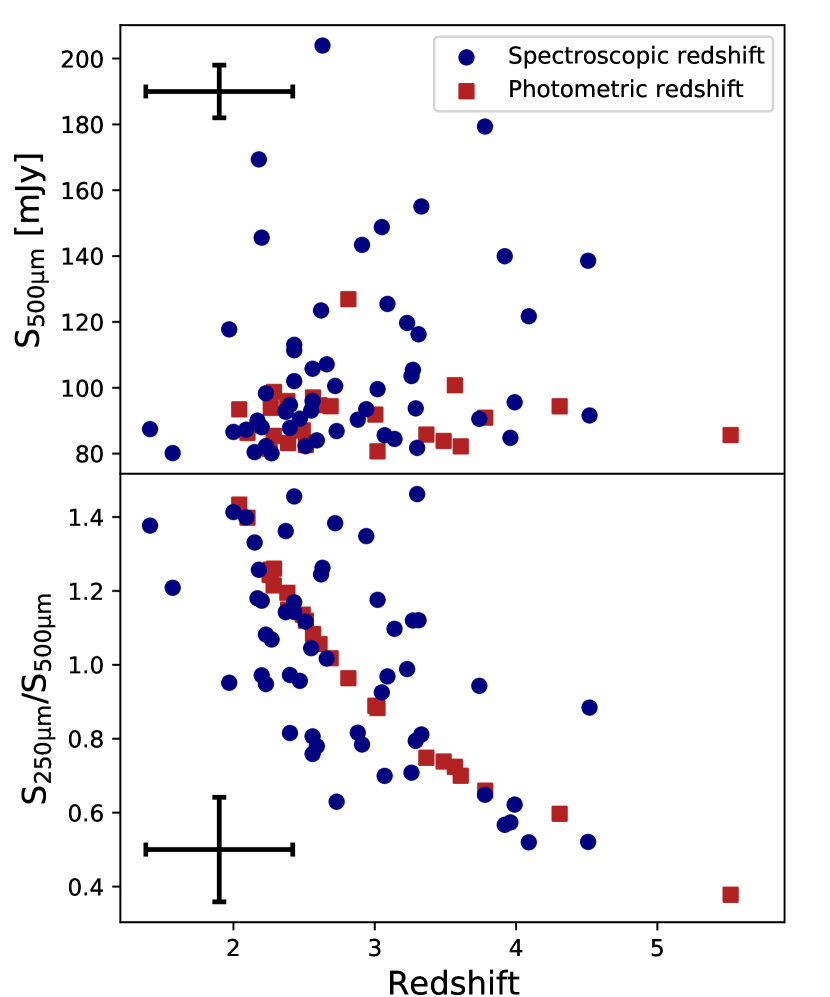
Figure 1: Top panel: 500 $\mu$m flux density against redshift. Sources with spectroscopic redshifts are shown as blue dots, while sources with only photometric redshifts are shown as red squares. Sources are selected with 500 $\upmu\mathrm{m}$ greater than 80 mJy. We show the typical uncertainties on these values in the top-left of the figure, assuming a $z_{\rm phot}=3$. For sources with multiple galaxies at different redshifts, we use the average spectroscopic redshift. Bottom panel: Submm colours and redshifts of our sample, illustrating the photometric selection function above $z_{\rm phot}=2$. Typical uncertainties in the colour and photometric redshift estimates are shown in the bottom-left of the graph.

Our targets are taken from the Herschel Astrophysical Terahertz Large Area Survey (H-ATLAS, Eales et al., 2010). H-ATLAS was the largest open-time key project on Herschel in terms of time awarded and legacy catalogue size, covering 550 deg², which was by far the widest area of any extragalactic Herschel survey. H-ATLAS mapped 150 deg² in the Northern Galactic Pole (NGP), three equatorial fields each of 36 deg² covering the Galaxy and Mass Assembly (GAMA) survey at RAs of 9h, 12h and 15h and two Southern Galactic Pole (SGP) fields of 102 deg² and 160 deg² respectively.

Our sample selection for this paper is based on the criteria set out in Bakx et al. (2018):

• $500$ $\upmu\mathrm{m}$ flux density $\geq 80$ mJy;

• Lack of cross-identification with known blazars or bright local galaxies (following the gravitational lens selection technique of Negrello et al., 2010);

• Photometric redshift estimate of $z_{\rm phot}\geq 2$ based on the Herschel SPIRE flux densities at $250$ $\upmu\mathrm{m}$, 350 $\upmu\mathrm{m}$ and 500 $\upmu\mathrm{m}$;

• Location in the H-ATLAS South Galactic Pole field.

The photometric redshift estimates were derived using the two-temperature modified black-body template from Pearson et al. (2013). In total, they find 209 sources, of which 88 were located in the SGP field, three of which already had spectroscopic redshifts at the start of our redshift campaign.

The spectral line survey was originally started as a pathfinder experiment with the ACA in Band 3 in Cycle 4 (in programme 2016.2.00133.S), and these Band 3 ACA observations were continued in Cycle 6 (in programme 2018.1.00804.S). An analysis after the Cycle 6 observations determined that more reliable redshifts could be measured by including Band 4 observations. This led to observations with the ALMA 12 m Array that covered all 85 fields in Band 4 as well as Band 3 (in programme 2019.1.01477.S) where emission lines were not already obvious.

All the sources with redshifts have band 4 observations using the ALMA 12 m array, with 74 sources also having band 3 observations using the 12 m array. Eleven sources, instead, rely on ACA observations in band 3. We find spectroscopic redshifts for one or multiple sources in 62 of the 85 Herschel fields. As reported by Bendo et al. in prep, we find 142 individual galaxies in the ALMA images, and here we report the 71 galaxies with spectroscopic redshifts. The targets are as presented in Table LABEL:tab:data_table (see Table A1 for integrated flux densities).

Figure 1 shows the submm colours of the 85 selected sources, and illustrates the selection function resulting from the flux limit and photometric redshift constraint. Of the 11 sources that rely on ACA data in band 3, 9 resulted in robust spectroscopic redshifts. This is a similar success rate as with the full baseline, and as such, we do not expect significant differences between the sources using ALMA full baseline array and ACA-dependent data. Note that the 2 mm and 3 mm integrated continuum flux density limits in our ALMA observations do not affect our sample selection in any way, because all targets were detected with continuum signal to noise ratios in excess of 8 at 3 mm and 10 at 2 mm (see Bendo et al., in prep.). This is also evident from Figure 1 in which no trends in redshift determination with colour or redshift are apparent.

Table 1: Sources with robust spectroscopic redshifts. (1) H-ATLAS source ID; (2) HerBS ID (Bakx et al., 2018) where available; (3) number of continuum sources; (4) source designation (section 2.1); (5) and (6) RA and Dec coordinates respectively; (7) spectroscopic redshifts obtained in this work; and (8) VIKING derived lens redshift from Bakx et al. (2020a).

H-ATLAS ID	HerBS ID	Number	Source	Coordinates (J2000)		$z_{\rm spec}$	$z_{\rm lens}$
		of sources	designation	RA	Dec
J012407.4$-$281434	11	1		01:24:07.50	$-$28:14:34.7	2.631
J013840.5$-$281856	14	1		01:38:40.41	$-$28:18:57.5	3.782
J232419.8$-$323927	18	1		23:24:19.82	$-$32:39:26.5	2.182	0.647
J234418.1$-$303936	21	2	[A+B]	23:44:18.11	$-$30:39:38.9	3.323
J002624.8$-$341738	22	2	A	00:26:24.99	$-$34:17:38.1	3.050
J004736.0$-$272951	24	1		00:47:36.09	$-$27:29:52.0	2.198
J235827.7$-$323244	25	1		23:58:27.50	$-$32:32:44.8	2.912
J011424.0$-$333614	27	1		01:14:24.01	$-$33:36:16.5	4.509
J230815.6$-$343801	28	1		23:08:15.73	$-$34:38:00.5	3.925	0.840
J235623.1$-$354119	36	1		23:56:23.08	$-$35:41:19.5	3.095
J232623.0$-$342642	37	1		23:26:23.10	$-$34:26:44.0	2.619	0.475
J232900.6$-$321744	39	1		23:29:00.81	$-$32:17:45.0	3.229	0.654
J013240.0$-$330907	40	1		01:32:40.28	$-$33:09:08.0	1.971
J000124.9$-$354212	41	3	A	00:01:24.79	$-$35:42:11.0	4.098
J000007.5$-$334060	42	3	[A+B+C]	00:00:07.45	$-$33:41:03.0	3.307
J005132.8$-$301848	45	3	A	00:51:32.95	$-$30:18:49.7	2.434
J225250.7$-$313658	47	1		22:52:50.76	$-$31:36:59.9	2.433	0.656
J230546.3$-$331039	49	2	[A+B]				0.620
			A	23:05:46.41	$-$33:10:38.1	2.724
			B	23:05:46.58	$-$33:10:43.1	2.730
J013951.9$-$321446	55	1		01:39:52.08	$-$32:14:45.5	2.656
J003207.7$-$303724	56	4	C	00:32:07.67	$-$30:37:34.3	2.561
J004853.3$-$303110	57	1		00:48:53.38	$-$30:31:09.9	3.265
J005724.2$-$273122	60	1		00:57:24.33	$-$27:31:23.3	3.261
J005132.0$-$302012	63	3	A	00:51:31.70	$-$30:20:20.6	2.432
J223753.8$-$305828	68	1		22:37:53.85	$-$30:58:27.9	2.719
J012416.0$-$310500	69	2	[A+B]
			A	01:24:16.16	$-$31:04:59.5	2.075
			B	01:24:15.87	$-$31:05:05.1	2.073
J012853.0$-$332719	73	1		01:28:53.07	$-$33:27:19.1	3.026
J005629.6$-$311206	77	2	[A+B]	00:56:29.25	$-$31.12:07.5	2.228
J230002.6$-$315005	80	3	[A+B]				0.651
			A	23:00:02.54	$-$31:50:08.9	2.231
			B	23:00:02.88	$-$31:50:08.0	1.968
J002054.6$-$312752	81	2	[A+B]
			A	00:20:54.20	$-$31:27:57.4	3.160
			B	00:20:54.74	$-$31:27:50.8	2.588
J235324.7$-$331111	86	1		23:53:24.56	$-$33:11:11.8	2.564
J005659.4$-$295039	90	2	A	00:56:59.28	$-$29:50:39.3	3.992
J234750.5$-$352931	93	1		23:47:50.44	$-$35:29:30.2	2.400
J233024.1$-$325032	102	2	A	23:30:24.43	$-$32:50:32.3	3.287
J225324.2$-$323504	103	1		22:53:24.24	$-$32:35:04.2	2.942	0.666
J001802.2$-$313505	106	2	A	00:18:02.46	$-$31:35:05.1	2.369
J014520.0$-$313835	107	1		01:45:20.07	$-$31:38:32.5	2.553
J223942.4$-$333304	111	1		22:39:42.34	$-$33:33:04.1	2.371	1.3
J000806.8$-$351205	117	2	A	00:08:07.20	$-$35:12:05.0	4.526
J012222.3$-$274456	120	2	[A+B]
			A	01:22:22.44	$-$27:44:53.7	3.125
			B	01:22:22.13	$-$27:44:59.0	3.124
J223615.2$-$343301	121	2	A	22:36:15.31	$-$34:33:02.3	3.741
J003717.0$-$323307	122	2	A	00:37:16.69	$-$32:32:57.4	2.883
J233037.3$-$331218	123	1		23:30:37.45	$-$33:12:16.8	2.170
J225339.1$-$325550	131	2	B	22:53:39.50	$-$32:55:52.3	2.197
J231205.2$-$295027	132	1		23:12:05.31	$-$29:50:26.5	2.473	0.652
J225611.7$-$325653	135	2	A	22:56:11.79	$-$32:56:52.0	2.401	0.640
J011730.3$-$320719	138	2	B	01:17:30.74	$-$32:07:18.0	1.407
J224759.7$-$310135	141	1		22:47:59.75	$-$31:01:35.7	2.085	0.653
J012335.1$-$314619	145	2	A	01:23:34.65	$-$31:46:23.6	2.730
J232210.9$-$333749	146	2	B	23:22:10.62	$-$33:37:58.4	2.003	0.760
J000330.7$-$321136	155	2	A	00:03:30.65	$-$32:11:35.1	3.077
J235122.0$-$332902	159	2	[A+B]
			A	23:51:21.76	$-$33:29:00.4	2.236
			B	23:51:22.36	$-$33:29:08.1	2.235
J011014.5$-$314814	160	1		01:10:14.46	$-$31:48:15.9	3.955
J000745.8$-$342014	163	3	A	00:07:46.24	$-$34:20:03.0	3.140
J225045.5$-$304719	168	2	A	22:50:45.48	$-$30:47:20.3	2.583	0.470
J011850.1$-$283642	178	4	[A+B+C]
			A	01:18:50.26	$-$28:36:43.9	2.658
			B	01:18:50.09	$-$28:36:40.6	2.655
			C	01:18:49.98	$-$28:36:43.2	2.656
J230538.5$-$312204	182	1		23:05:38.80	$-$31:22:05.6	2.227	0.778
J234955.7$-$330833	184	1		23:49:55.66	$-$33:08:34.4	2.507
J225600.7$-$313232	189	1		22:56:00.74	$-$31:32:33.0	3.300	0.672
J014313.2$-$332633	200	1		01:43:13.30	$-$33:26:33.1	2.151
J005506.5$-$300027	207	1		00:55:06.51	$-$30:00:28.3	1.569
J225744.6$-$324231	208	2	[A+B]
			A	22:57:44.59	$-$32:42:33.0	2.478
			B	22:57:44.83	$-$32:42:32.8	2.483
J224920.6$-$332940	209	2	A	22:49:21.04	$-$33:29:41.5	2.272	0.508

2.2 ACA observations

Data were acquired with the ACA (also called the Morita Array) during ALMA Cycles 4 and 6 in programmes 2016.2.00133.S and 2018.1.00804.S (P.I.: S. Serjeant). Some details about these observations are listed in Table 2. The observations of each target consisted of single pointings with a series of 5 spectral tunings set up to cover the sky frequency range between 86.6 and 115.7 GHz (2.59 - 3.46 mm; Fig. 2 top panel). Each spectral tuning consisted of four spectral windows that were 2 GHz ($\sim$5500 km s^-1) in size, with two spectral windows placed adjacent to each other in a lower sideband and two more in an upper sideband, with the sidebands separated by 8 GHz. Not all observations with all spectral tunings were executed in Cycle 4. For some targets, however, line emission was detected using the limited Cycle 4 data that were acquired. For these sources, we did not request any additional Cycle 6 observations to complete the coverage of the 86.6 to 115.7 GHz range. Typically, several targets located close to each other in the sky were observed with the same spectral settings within one Execution Block, and thus the sources share bandpass, flux density, and phase calibrators. The calibrators were typically quasars, although Solar System objects were used for flux calibration in some observations.

Our spectral coverage allows us to detect CO lines between the (2$-$1) and (6$-$5) transitions depending on the redshift of the sources as seen in Figure 2. In addition, we can also potentially detect the [CI](${}^{3}\rm P_{1}-^{3}\rm P_{0})$ fine-structure line at 492 GHz for z=3.3-5.7 sources and the [CI](${}^{3}\rm P_{2}-^{3}\rm P_{1})$ at 809 GHz for z=7.0-9.3 sources. Given the redshift range of the sources, other molecular lines might be expected (e.g., H₂O, HCO⁺, HCN, CN, Spilker et al., 2014), but these would not be detectable in our data given the limited observation time per source. The CO and [CI ] lines covered in the 86.6$-$115.7 GHz range would allow us to measure spectral lines between $0.0<z<0.3$, $1.0<z<1.7$, or $2.0<z<9.6$.

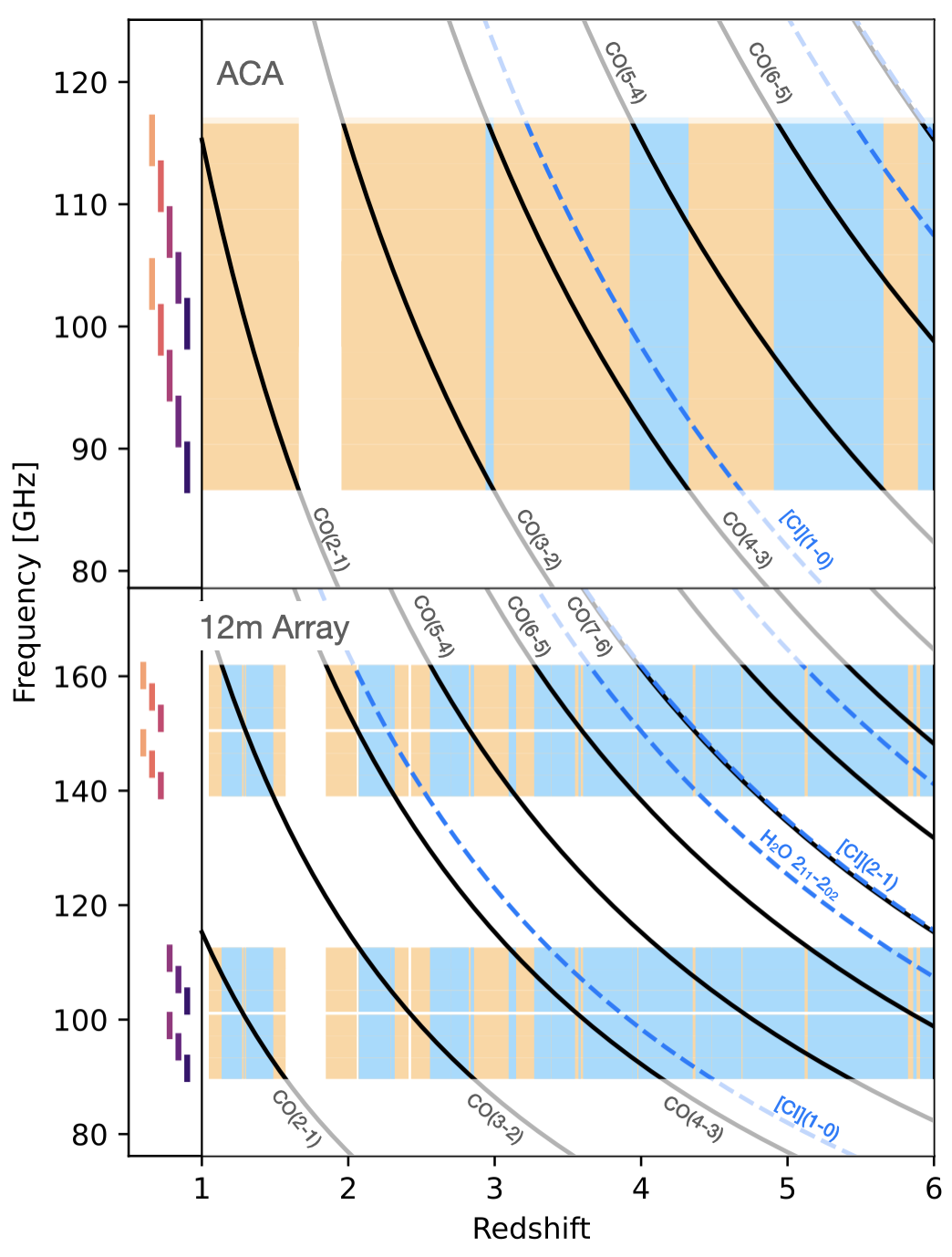
Figure 2: Redshift as a function of frequency for the ACA Band 3 spectral coverage (86.6-115.7 GHz; top panel) and ALMA 12-m Array (89.6-112.6 and 139-162 GHz; bottom panel) for the ${}^{12}\rm CO$ (solid black lines), C i and water (dashed blue lines) emission lines. The blue areas identify the redshift range where at least 2 CO emission lines fall within this frequency range, and the orange areas show where only one CO line falls within the frequency range. “Redshift deserts" are shown as white areas. The coloured bars at the left-hand side of the plots show the location of the spectral tunings that were used for the ACA and 12-m Array. Our 12-m Array tunings (Section 2.3) dramatically improved our ability to find robust redshifts drastically from an estimated 12 to 90 per cent using only one extra tuning.

The sensitivity goals were set to 3 mJy, as measured within a velocity width of 308 km s^-1, since this was the expected line width of the data; this was typically matched by our observations. Our sensitivity goal was determined by the relationship between bolometric ($40-500$ $\upmu\mathrm{m}$) and CO luminosities (Solomon & Vanden Bout, 2005), where, for the purposes of observation planning, no correction was made for differing excitation of CO lines (Bothwell et al. (2013) and references therein). For the transitions in the Band 3 window ($84-116$ GHz), we predicted CO fluxes of $4.6-8.0$ Jy km s^-1 for our targets, which is consistent with our CO detections of H-ATLAS lensed galaxies to date (e.g., Neri et al., 2020) and broadly consistent with the predictions of Combes et al. (1999) once the latter is scaled to our H-ATLAS fluxes. The spectral resolution was set to 7.813 MHz, which is equivalent to a velocity bin of $20-25$ km s^-1. These channels could be binned as needed to improve the detection of the line emission.

2.3 12-m Array observations

Data were acquired with the ALMA 12-m Array during ALMA Cycle 7 in programme 2019.1.01477.S (P.I.: S. Urquhart). Each field was observed in Bands 3 (if it had not been observed with the ACA in this band) and 4 using a single pointing with the 12-m Array in either the C43-1, C43-2, or C43-3 configurations. These configuration yielded beams with full width at half-maxima (FWHM) of approximately 3 arcsec in Band 3 and 2 arcsec in Band 4. Additional details of the observations are listed in Table 2. Note that these configurations are sufficient for detecting line emission, which was the primary intention of this programme, and the configurations can also be used to resolve Herschel sources into multiple individual galaxies; however, most of the detected targets will be unresolved point sources.

The observations used six spectral tunings with three in each band, as shown in Figure 2. These observations produce near-continuous coverage of 23.25 GHz bandwidth centred at 101 and 151 GHz (89.6$-$112.6 and 139$-$162 GHz). We based the precise tunings in Bands 3 and 4 on the method detailed in Bakx et al. (2020c), where we optimised the expected number of sources with robust redshifts (x, two or more spectral lines) assuming that the proposed sources follow the existing redshift distribution of Herschel-selected galaxies (Bakx et al. 2018; Bakx et al. 2020c; Neri et al. 2020 and references therein). We derive this optimised solution using a Monte-Carlo approach, where we generated 1000 fake redshift catalogues of 1000 redshifts, drawn from the previously-mentioned redshift distribution assuming a standard error of $\Delta z/(1+z)=0.13$ (e.g., Pearson et al. 2013; Ivison et al. 2016). We test all potential ALMA tuning configurations using between four and eight ALMA tunings, placed randomly across Bands 3 to 6.

This optimisation indicated that stacking the tunings to create a continuous coverage is always favoured. The typical ALMA tuning used in studies such as Weiß et al. (2013) and our earlier ACA data — to essentially fully cover Band 3, as in the top panel of Figure 2 — was found to be particularly good at detecting at least one spectral line (an expected 87 per cent across our sample). However, this approach is rather inefficient given the large overlap between the upper sidebands of the lower-frequency tunings and lower sidebands of the higher-frequency tunings. Similarly, this set-up only results in a robust multi-line detection for galaxies beyond redshift 3.5 (an expected $\sim$12 per cent of our sample). Instead, two sets of three tunings in Bands 3 and 4 significantly increased the number of sources with robust redshifts to an expected 65 per cent, and it diminished the size of the redshift desert around redshift 2. An added benefit from this larger per centage of robust redshift detections, is that we can exclude redshift solutions where we would have detected more than one line. In fact, we can identify the spectroscopic redshifts of sources robustly with just a single line, by excluding redshift solutions that would have resulted in multi-line detections. In other words, if we would have detected two spectral lines within our covered bandwidth for every redshift solution except one, we can identify the redshift robustly from a single bright detected spectral line. This method is explained in more detail in Bakx et al. (2020c), and a dedicated discussion of this method will be presented in Bakx et al. in prep.. In total, this statistical exercise raised the probability for detecting robust redshifts (both by multiple spectral line, and by inference) from 12 per cent to 90 per cent while only requiring 20 per cent extra observation time for the additional band 4 tuning. Based on the results of the ACA campaign described above, we required an RMS of 0.8 mJy for a 300 km s^-1 line; this was typically matched by our observations.

2.4 Data processing

The 12-m Array data were pipeline-calibrated with the Common Astronomy Software Applications (CASA) package version 5.6.1 (McMullin et al., 2007), while the ACA data were manually calibrated with the same version of CASA. In both cases, the first steps of the calibration of the visibility data included amplitude corrections based on the system temperature and antenna position corrections. Phase corrections based on water vapour radiometer measurements were also applied at this point to the 12-m Array data only. After this, we flagged shadowed antennas and channels with low sensitivities at the edges of the spectral windows. In the ACA data, we also visually inspected the data and flagged any data where the amplitude gains were outliers, where the amplitudes varied irregularly across the spectral window, or where the phases show jumps between observations or unusually high scatter. For both the ACA and 12-m Array data, we then calibrated the amplitudes and phases both as a function of channel and as a function of time. The uncertainty in the flux calibration is 5 per cent (Remijan, 2019).

Imaging was done with the tclean command within CASA version 5.6.1. Slightly different settings were used for the Band 3 ACA data, the Band 3 12-m Array data, and the Band 4 12-m Array data, and these different settings are listed in Table 2. All images were created using natural weighting, the standard gridder, and the Hogbom deconvolver. The pixel scale was set to so that the full-width at half-maximum (FWHM) of the beam was sampled by at least three pixels, and the image size was set to cover the area over which the primary beam is $>$0.20$\times$ the peak value. Spectral lines were initially identified in the image cube without continuum subtraction. Once spectral lines were found, the continuum was subtracted from the visibility data, and the data were re-imaged with manual adjustments made to the channel width in the final image cubes to optimize the balance between the sampling of the spectral line emission and the signal-to-noise ratio (as measured in both the individual image slices and the extracted spectrum).

Table 2: ALMA image characteristics.

Array	Band	Central	Total	Typical	Pixel	Image size
		frequency	bandwidth	beam FWHM	scale	[pixels]	[arcsec]
		[GHz]	[GHz]	[arcsec]	[arcsec]
ACA	3	101	29.1	17 $\times$ 10	2.0	100 $\times$ 100	200 $\times$ 200
12-m Array	3	101	23.25	3.6 $\times$ 2.7	0.5	240 $\times$ 240	120 $\times$ 120
12-m Array	4	151	23.25	2.2 $\times$ 1.8	0.3	240 $\times$ 240	72 $\times$ 72

3 Spectroscopic Redshifts

3.1 Line extraction

Line measurements were made using aperture photometry within the image cubes. Lines were first identified by visual inspection of the data independently by several of the authors, and then confirmed through the following process. Circular apertures were centered on the peaks of the corresponding continuum emission, and the radii of the apertures were manually adjusted for each source in each image to include as much line emission as possible while still measuring that emission at higher than the 5$\sigma$ level. Similarly, we manually selected frequency channels that measured as much of the line flux as possible without diluting the signal with background noise so much that the measurements fall below 5$\sigma$. Note that the continuum is detected at a higher S/N than the line emission. If we matched the apertures used to measure the continuum and line emission, we would either need to choose large apertures that included all of the detectable continuum emission but also included extra noisy pixels for the line emission or small apertures that optimize the line detections but do not include all of the continuum emission.

3.2 Redshift determination

With the precise frequencies of the spectral lines in hand, we calculate all potential redshift solutions for each line, and use the method described in Bakx et al. (2020c) to provide only robust redshifts. This method accounts for any sources that could be influenced by the redshift degeneracy that can affect the linear CO-ladder. In total, we find redshifts for 59 sources using multiple spectral lines that point to an unambiguous redshift solution. Meanwhile, this method also provides additional information. For thirteen sources, we find bright emission from only a single line. In these specific cases (HerBS-22, -39, -40, -60, -73, -80B, -81A, -103, -122A, -146B, -155 and -207, -208B), we are able to exclude all other redshift solutions. The exclusion of redshift solutions requires us to be confident that lines are indeed non-existent. Since adjacent CO spectral lines typically have similar integrated line fluxes, we can only exclude redshift solutions for galaxies with strong line detections in CO lines.

We note that the uncertainty of the spectroscopic redshifts is less than 0.001, however for clarity, we show only three trailing digits in Table LABEL:tab:data_table. For the SGP field, data were taken from H-ATLAS SGP Data Release 2 Catalogue version 1.4 (Smith et al., 2017; Maddox et al., 2018; Furlanetto et al., 2018). There are fields where we have detected multiple sources. In these cases, we have labelled them alphabetically with decreasing brightness and quoted redshifts for the sources where we were able to robustly detect them. Details on the continuum measurements, including information on additional sources detected only in continuum emission, will be given in Bendo et al. (in prep). In cases where our lowest angular resolution does not resolve the source into separate components, we only provide the redshift of the system, denoted by straight brackets (e.g., HerBS-21 [A+B] at $z_{\rm spec}=3.323$).

In total, across our 71 galaxies with robust redshifts (associated with 62 Herschel sources, Table 1), we find the following lines robustly (for upper limits we refer to the upcoming paper by Hagimoto et al.). We primarily detect CO(3$-$2), (4$-$3) and (5$-$4) emission (38, 36 and 28 sources, respectively), with only a handful of sources with CO(2-1), CO(6-5) and CO(7-6) emission (two, nine and four, respectively). For 21 galaxies we find CI(${}^{3}\rm P_{1}-^{3}\rm P_{0}$) emission, for one galaxy CI(${}^{3}\rm P_{2}-^{3}\rm P_{1}$) emission, and one galaxy shows H₂O 2₁₁-2₀₂ emission. We detail the line fluxes in Table LABEL:tab:lines, and the lines can be seen graphically in Figure 3. Here we note that these individually-resolved components are likely to be individual galaxies (e.g., Hayward et al. 2013). However, it is possible that a small fraction are multiple images of the same galaxy system lensed by foreground cluster lenses. The exact nature of the individual components (among which are protocluster cores; e.g., Oteo et al. 2018) will be discussed more in upcoming papers. Multiple images in galaxy-galaxy gravitational lensing systems would not be resolved in our ALMA data, since for source redshifts $\gg$ lens redshifts, the critical radius in a Singular Isothermal Sphere lens asymptotes to $\sim 1.5^{\prime\prime}\times(\sigma_{\rm v}/230$ km s${}^{-1})^{2}$ where $\sigma_{\rm v}$ is the lens velocity dispersion.

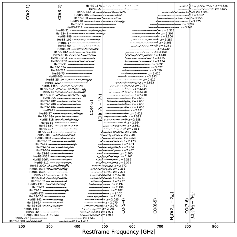
Figure 3: ALMA spectra of the 71 galaxies with spectroscopic redshifts reported in this paper shown at their rest-frame frequency, offset vertically for clarity. Vertical lines indicate the transitions of CO, H₂O and C i lines. The sources are ordered by redshift and the flux scaling for each spectrum is arbitrary. The optimised 3- and 2-mm band tunings resulted in a successful redshift identification for the majority of sources.

3.3 Sources without robust redshifts

We were unable to identify the redshifts for 23 Herschel sources with the ALMA 12m-Array data. Only for five of these sources did we not detect any line emission, indicative that our true redshift desert is relatively small. For seven of these targets, we did not deem the main line bright enough to use the exclusion method to remove any of the adjacent redshift options (two of which had ACA Band 3 observations instead of from the ALMA 12m-Array). Nine targets have suggestive secondary lines, although none of them are above the 5$\sigma$ threshold to result in a redshift detection, and finally, seven sources have only a single line observed, with no ability to exclude any nearby redshift solutions, and thus remain ambiguous in their redshift solution. The objects without redshifts do not otherwise appear to be atypical of our sample, as can be seen in Fig. 1 and Bendo et al. in prep. We are currently underway with, and planning future follow-up observations to reveal the redshifts of these remaining 23 sources, and will provide the complete catalogue of redshifts in a future work.

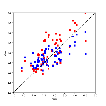
Figure 4: Comparison of the spectroscopic redshifts presented here with the photometric redshifts from Bakx et al. (2018) shown in red and from Ivison et al. (2016) shown in blue. Our results are consistent with the spread seen in, e.g., Ivison et al. (2016), Bakx et al. (2018), Pearson et al. (2013). Note that this diagram is necessarily restricted to objects with spectroscopic redshifts.

3.4 Spectroscopic versus photometric redshifts

Fig. 4 presents a comparison of the photometric redshifts from previous catalogues in Bakx et al. (2020b) which use an SED fit and the method described in Ivison et al. (2016) to the spectroscopic measurements presented here, showing a dispersion similar to the ones seem in Ivison et al. (2016) and Bakx et al. (2018). For Herschel sources with multiple components at the same redshift (HerBS 49, 69, 120, 159, 178 and 208), we show the weighted average of the spectroscopic redshift against the photometeric redshift estimate. The two sources with multiple components at different redshifts are excluded in this figure. We find similar uncertainties on the submm photometric redshifts as previously reported in Pearson et al. (2013); Ivison et al. (2016); Bakx et al. (2018); Jin et al. (2019). The average difference between $z_{spec}$ and $z_{phot}$, $\Delta z$, for the two samples are $\Delta z_{\rm Bakx}$= 0.469 and $\Delta z_{\rm Ivison}$= 0.388. The standard deviations are $\sigma(\Delta z_{\rm Bakx}/(1+z_{\rm spec}))=0.14$ and $\sigma(\Delta z_{\rm Ivison}/(1+z_{\rm spec}))=0.13$. Paper II (Bendo et al. in prep.) will present a more exhaustive analysis of the continuum spectral energy distributions and the photometric redshifts.

3.5 Comparison to foreground lens redshifts

Foreground lens redshifts and morphologies are the subject of multiple ongoing optical and near infrared imaging and spectroscopy campaigns with HST (e.g., Berta et al. 2021, see also Borsato et al. in prep.), Spitzer and large ground-based telescopes (e.g., VLT and Keck). Submm-selected strong lens candidates are found purely on the basis of the magnification bias, and unlike optically-selected or radio-selected lenses, the selection is independent of lensing morphology, lensing galaxy properties, or the presence of emission lines in the background source. This relatively clean magnification-based lensing detection, together with the negative submm K-correction that permits detection of background sources to $z=5$ and beyond, means that we are sensitive to foreground lenses out to $z\sim$2 and therefore, these follow-up programmes can be used to probe the evolution of stellar and halo mass distributions. For sources where the data currently exist, we compare our spectroscopic lensed redshift values with those of proposed foreground lensing galaxies taken from Bakx et al. (2020a), derived from the VISTA Kilo-degree Infrared Galaxy (VIKING) survey (Edge et al., 2013), a survey in zYJHK_S to sub-arcsecond resolution. This survey overlaps with both the equatorial GAMA fields and the Southern Galactic Pole (SGP) fields and thus covers a number of the H-ATLAS sources. At the time of writing, however, no VIKING catalogue has been published over the whole SGP and GAMA fields. For the 98 HerBS sources in their sample, Bakx et al. (2020a) found probable lenses for 56 and showed that, within 10 arcseconds, 82 per cent of the HerBS sources have associated foreground VIKING galaxies. Table LABEL:tab:data_table gives the probable lens redshifts applicable here and, as expected, they all have lower photometric redshifts than the sources we present.

4 Discussion

4.1 Redshift and CO line width distributions

We derived CO brightness estimates via equation 3 of Solomon & Vanden Bout (2005):

$$\frac{L^{\prime}_{\rm CO}}{\rm K\,km\,s^{-1}\,pc^{2}}=3.25\times 10^{7}\times\\ \frac{S_{\rm CO}\Delta v}{\rm Jy\,km\,s^{-1}}\left(\frac{\nu_{\rm obs}}{\rm GHz}\right)^{-2}\left(\frac{D_{\rm L}(z)}{\rm Mpc}\right)^{2}(1+z)^{-3},$$ (1)

where $D_{\rm L}$ is the luminosity distance to redshift $z$, $\Delta\nu$ is the linewidth, $\nu_{\rm obs}$ is the observed frequency, and $S_{\rm CO}$ is the observed line flux. Figure 5 shows the distribution of redshifts and line widths (FWHM) for the 71 galaxies with robust spectroscopic redshifts from this work. We compare them against two samples, roughly divided into a lensed and unlensed sample. The lensed sample is compiled from Neri et al. (2020), Harris et al. (2012), Yang et al. (2017), Aravena et al. (2016) and some well known individual sources. These are the lensed sources known as IRAS FSC 10214+4724 (e.g., Rowan-Robinson et al., 1991; Serjeant et al., 1995; Eisenhardt et al., 1996), the Cosmic Eyelash (Swinbank et al., 2010), the Cloverleaf Quasar (e.g., Magain et al., 1988; Barvainis et al., 1994; Solomon et al., 2003), APM 08279+5255 (e.g., Irwin et al., 1998) and the Cosmic Eyebrow (e.g., Dannerbauer et al., 2019). The unlensed sample comes from Bothwell et al. (2013), Harris et al. (2010) and several well known individual unlensed sources from literature. These are the sources known as BR 1202$-$0725 (N and S) and BRI 1335$-$0417 (Carilli & Walter, 2013; Dannerbauer et al., 2019), along with two binary hyper-luminous galaxies: HATLAS J084933+021443 ($z$=2.41, Ivison et al., 2013) and HXMM01 ($z$=2.308, Fu et al., 2013).

The redshift distribution of our sample has a mean redshift of 2.75 and median redshift of 2.61, with all sources lying within the redshift range $1.41<z<4.52$. For 67 of the sources, the exceptions being HerBS-40 ($z=1.971$), HerBS-80B ($z=1.968$), HerBS-138B ($z=1.41$) and HerBS-207 ($z=1.57$), we find redshifts above 2, which we would expect due to the photometric redshift pre-selection. The mean redshifts of these lensed and unlensed comparison samples are 3.04 and 2.65, respectively.

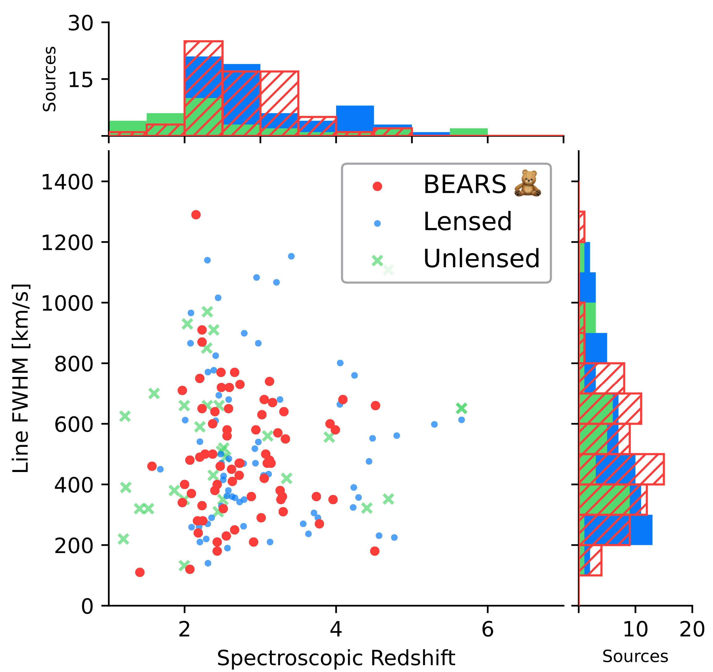
Figure 5: Distribution of the spectroscopic redshifts and linewidths of the 71 BEARS galaxies presented in this work, compared to the samples described in the text.

The mean line width (FWHM) distribution is also shown in Fig 5. We find a median width of 475 km s^-1 and a mean of 494 km s^-1, which lies below both the values of the lensed and unlensed samples reported which are 524 km s^-1 and 577 km s^-1 respectively, the median values are 496 km s^-1 (lensed) and 531 km s^-1 (unlensed). As we will discuss later, this is consistent with their lensing nature and we will discuss the physical interpretation of this, including their complex dynamics in subsequent sections.

4.2 The $L^{\prime}_{\rm CO}$ and $\Delta V$ relation

Bothwell et al. (2013) noted that the CO luminosities of submillimetre galaxies correlate with their line widths, which they interpreted as baryon-dominated gas dynamics. This relation extends a similar trend seen in molecular clouds (Bolatto et al., 2008). Lensed submillimetre galaxies occupy a different region of this relation, as noted by Harris et al. (2012), due to magnification effects predominantly affecting the luminosities and not line widths.

The ¹²CO (1-0) luminosities of our sample were calculated following the standard relation of Solomon & Vanden Bout (2005) (Eq. 1). The results are presented in Fig. 6 and show the relationship between apparent CO luminosities and the FWHM of the CO emission line, $\Delta V$ including data from a number of other studies. We use the previously defined “lensed" and “unlensed" samples (Section 4.1) and create an additional sample of ULIRGS. This is composed of data from Solomon et al. (1997), Combes et al. (2011) and Combes et al. (2013). The values of the CO luminosities used in this paper are explicitly for CO(1$-$0), $L^{\prime}_{\rm CO(1-0)}$, in order to make a direct comparison with the majority of quoted literature values, a correction for excitation was applied using the median brightness temperature ratios for SMGs in Table 4 of Bothwell et al. (2013), and accounting for errors. We calculate the CO(1$-$0) luminosity from the lowest CO transition available. For a minority of cases, where sources in the literature were not given as ${}^{12}\rm CO(1-0)$, the appropriate corrections (as already described) for excitation were applied. It should be noted that none of these (likely) gravitationally lensed sources are corrected for the effects of lensing magnification.

Including our sources in this diagram does not alter the observed trend reported in Neri et al. (2020) and also seen in, for example, Harris et al. (2012) whereby there is a clear distinction between sources that are strongly lensed and those that are unlensed.

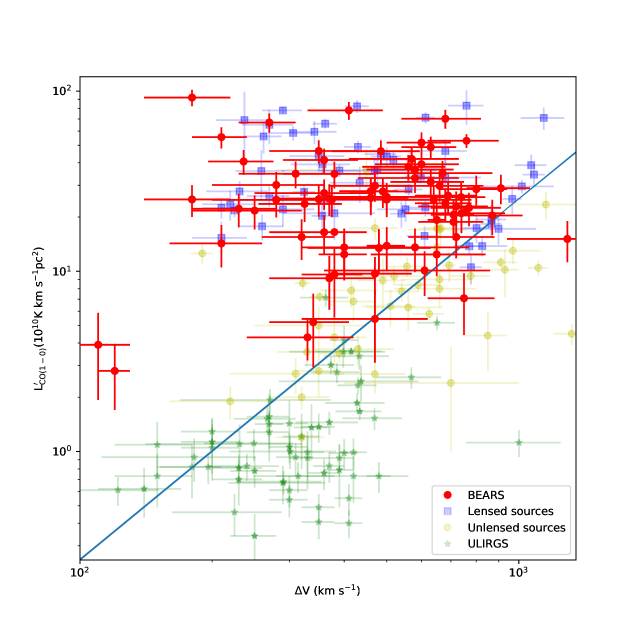
Figure 6: Apparent CO luminosity ($L^{\prime}_{\rm CO(1-0)}$) versus linewidth ($\Delta V$) for the sources identified in this work, along with sources from literature. Shown are both high-redshift lensed and unlensed samples (see Section 4.1 for more details) and a sample of ULIRGS (see Section 4.2 for more details). A trend line for the unlensed population is also shown.

4.3 ALMA as an efficient redshift hunter

Our Bands 3 and 4 observations with ALMA identified the redshifts for 71 galaxies, based on the initial positions of 62 Herschel sources (Table 1). We did not find robust redshifts for 23 Herschel sources, although two of those only had Band 3 data from ACA. Using our bespoke tuning set-up, we have a success-rate of 75 per cent ($=62/[62+23-2]$) which is lower than the initial 90 per cent promised by our simulations (see Section 2.3). As discussed in Section 3.3, only seven sources have single lines detected without the ability to exclude any nearby redshift solutions. Deeper observations promise to improve this fraction to 92 per cent ($=[85-7]/[85]$), given that we failed to use our exclusion method on seven sources, and nine sources had low-significance line features that were below our line detection criteria. The low-significance line features may be partially due to the large multiplicity found for many of our sources (see Bendo et al. in prep. for more details). Here, we also note, however, that this 92 per cent estimate might have been optimistic, since: (1) two sources were observed with the full five-tuning Band 3 coverage in ACA before a three-tuning follow-up in Band 4 using the 12-m Array; and (2) some of the nine sources with faint line emission might have redshifts that still prove ambiguous even with deeper observations, because sometimes the limiting factor is spectral coverage rather than signal-to-noise.

4.4 The effects of differential magnification on luminosities

Could differential magnification affect the observed distribution of magnification factors evident in Fig. 6? Whilst gravitational lensing is a purely geometrical effect, and as such is independent of wavelength, the degree of magnification will vary depending upon the line of sight. For example, an extended background source may exhibit intrinsic colour gradients, and the magnification may vary across the resolved background source. Therefore a lensed source and an unlensed source may have differing colours when averaged over the system. This is “differential magnification", potentially significantly affecting broad-band photometry and crucial emission line diagnostics (Serjeant, 2012). It is often assumed that this effect can be neglected, but here we would like to justify why this is an acceptable assumption to make in this paper.

We have repeated the methodology of Serjeant (2012) (to which the reader is referred for more details) to run a simulation of a $z=2.3$ background galaxy with a foreground gravitational lens at $z=0.9$. The background source structure was modelled on the original Swinbank et al. (2010) observations of the Cosmic Eyelash lens system, with four giant star-forming clumps, selected as an ostensibly typical example of the submm galaxy population. This is shown in Fig. 7. The $1\sigma$ spread in differential magnification effects are at around the 20 per cent level.

However, since the Swinbank et al. (2010) Submillimeter Array (SMA) observations of the Cosmic Eyelash, Ivison et al. (2020) using ALMA found a much smoother dust continuum and suggested that the SMA structures were artefacts of using CLEAN to image low signal-to-noise data, an issue that did not affect the images created from the ALMA data. The  $\sim\!\pm 20\%$ systematic in Fig. 7 is therefore the most pessimistic case. In order to quantify the effect of more smoothly distributing the star formation, we performed a new set of simulations with star formation contained in 100 giant molecular clouds, rather than four, again following the methodology of Serjeant (2012). This is shown as the red curve in Fig. 7, and is a $\pm 3.5\%$ effect. The differential magnification effects are larger when the CO emission is more concentrated, because it is easier for a large proportion of the CO flux to be close to a caustic curve.

In summary, the worst case is that the differential magnification effects are comparable to or smaller than the random errors, while in more realistic up-to-date models the effects in this case are negligible. We conclude that we can reasonably neglect differential magnification effects for the CO lines in this paper.

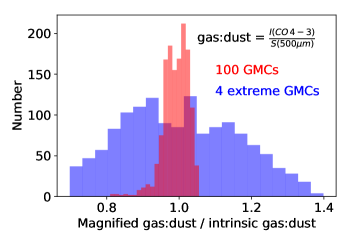
Figure 7: Simulation of differential magnification effects on a submm galaxy at $z=2.286$ lensed by a $z=0.9$ foreground galaxy. The blue histogram shows random realisations assuming the star formation is confined to only four giant molecular clouds as claimed originally for the Cosmic Eyelash by Swinbank et al. (2010), while the red histogram with narrower bins shows the distribution of random lensing realisations with star formation distributed over 100 identical molecular clouds, as suggested by the smooth continuum observed by Ivison et al. (2020). Note the much narrower distribution when the star formation is spread more uniformly throughout the system (red), and the wider distribution when the star formation is concentrated into a very small number of clumps (blue).

4.5 Magnification distribution

The vertical offset of lensed sources in Fig. 6 is due to gravitational magnification, which in turn depends only on the lensing geometry and is therefore formally independent of velocity width $\Delta V$. This figure can therefore be used to make magnification estimates. The magnifications from the offset from our fit to the unlensed samples are listed in Table LABEL:tab:MagnificationFactors.

The underlying magnification probability distribution generically tends to follow a $\Pr(\mu,z)\mathrm{d}\mu=a(z)\mu^{-3}\mathrm{d}\mu$ power law (Blain, 1996; Serjeant, 2014), but this is then convolved with the luminosity function, so the resulting magnification distribution may not necessarily be representable by such a simple power-law function. Therefore, a lensing population model is required.

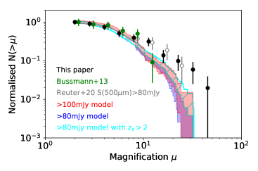
Figure 8: Observed cumulative magnification distribution of lensed submm galaxies (magnifications $\mu\geq 2$) with redshifts from this paper, compared to the LensPop submm population discussed in the text with a flux limit of $>100$ mJy (red) and $>80$ mJy (blue), and with a HERBS-like additional selection of source redshift $z_{\mathrm{source}}>2$ (cyan hatched). The shaded areas represent the Poisson uncertainties in the numbers from the model realisations. Note the good agreement between data and models over most of the magnification range, but the hint of an excess at large magnifications. Also shown is the magnification distribution from the 500 $\upmu\mathrm{m}$-selected sample of Bussmann et al. (2013), and the South Pole Telescope targets with $\geq 80$ mJy at 500 $\upmu\mathrm{m}$ and with modelled magnifications (Reuter et al., 2020), though note that the latter data points have flux limits at a total of three wavelengths so are not straightforwardly comparable.

The model used as the basis for the work presented in this section was described in Collett (2015) with its source code available as open source software, and was originally designed to predict strong gravitational lensing of optical galaxies. As described in that paper, the code was verified against observations of lenses by the galaxy-scale search of the Canada-France-Hawaii Telescope Legacy Survey (More et al., 2012; More et al., 2016; Gavazzi et al., 2014). The paper predicted lenses discoverable by the Wide Field Survey of Euclid (Laureijs et al., 2011), the Dark Energy Survey (Treu et al., 2018) and the Rubin Observatory (Ivezic et al., 2008). The model was used in Weiner (2019) to predict $122$ strong galaxy-galaxy lenses in COSMOS, in broad agreement with the 23 highly likely lenses and 159 lens candidates in that field (Faure et al., 2008; Jackson, 2008), to make predictions for the Euclid Deep Fields and to examine dependencies on cosmological parameters. A further prediction of $\geq$17 000 lenses discoverable by the Nancy Roman Space Telescope (Green et al., 2012) was presented in Weiner et al. (2020).

The model assumes strong lensing by elliptical galaxies, modelled as singular isothermal ellipsoids (SIEs). A population of foreground SIEs is generated with five key parameters: redshift, stellar velocity dispersion, flattening, effective radius and absolute magnitude. The lensing cross-section of the foreground population is then projected onto a selected background source population to generate an idealised set of lens systems (deflector + source). Finally, the model applies criteria based on the observing parameters of the survey being considered in order to discover the final set of strong lenses detectable by that survey.

To adapt the model for use in predicting lensing of submillimetre galaxies, we have made two major changes: firstly, a source catalogue of submillimetre galaxies was needed to replace the source catalogue of optical galaxies originally used; secondly, the criteria used to detect the lenses were altered. A mock submillimetre catalogue was created, based on the study by Cai et al. (2013) that allows for an estimate of number counts as a function of the (unlensed) flux at 500 $\upmu\mathrm{m}$ and redshift. For simplicity, we have used only submillimetre galaxies at $z>1$, and require that the background source lies within the Einstein radius in order for strong lensing to be possible. The LensPop model also requires the source galaxy angular size, which we have estimated using data from Ikarashi et al. (2015, figure 6: $z\sim 1-3$ and $z>3$ only). The source density parameter was calculated from the data in Cai et al. (2013) to be 0.011 arcsec^-2. The criterion for strong lens detection was simply that the 500 $\upmu\mathrm{m}$ flux density be greater than the chosen flux limit, replacing the seeing and signal-to-noise criteria of Collett (2015). A total of 10 per cent of the sky was simulated, to avoid Poisson errors in the models dominating the comparison with the data. A further simulation of $10\%$ of the sky was undertaken, from which a HERBS-like subset of source redshift $z_{\mathrm{source}}>2$ was selected.

Figure  8 shows the results of this modelling, compared to our observations. The flux density limit of $80$ mJy applies to the targets in this paper, but we have included a $100$ mJy prediction to demonstrate robustness to the precise choice of flux limit. The imposition of a HERBS-like $z_{\mathrm{source}}>2$ cut has a small effect on the magnification distribution. The HERBS-like selection (cyan in Fig. 8) agrees well with the observations out to magnifications of $\sim 10$, but there are hints of an excess of objects at higher magnifications. Also shown are the magnifications of a 500 $\upmu\mathrm{m}$-selected sample measured in interferometric mapping by Bussmann et al. (2013), and the magnifications estimated for South Pole Telescope targets that have 500 $\upmu\mathrm{m}$ fluxes above $80$ mJy and individual magnifications derived from lens modelling (Reuter et al., 2020), although note that this latter sample also has $1.4\,$mm and 870 $\upmu\mathrm{m}$ flux cuts so is not straightforwardly comparable.

There are at least three potential explanations. One possibility is that uncertainties in the magnification cause an Eddington-like bias in the magnification distribution in Fig. 8, and indeed Aravena et al. (2016) find that these magnification estimates can have large uncertainties; interferometric mapping will help determine whether this is the case. A second possible explanation is that this could indicate an additional contribution to the gravitational lensing optical depth that is not captured by the LensPop modelling. This model only considers galaxy-galaxy lensing, and has no contribution from strong lensing by galaxy clusters. There are other indications that the contribution from galaxy group or cluster lensing is not insignificant for wide blank-field surveys, as the measurement of a strong magnification bias (González-Nuevo et al., 2017; Dunne et al., 2020) or the fact that the submm–K-band offsets in Bakx et al. (2020a) are larger than the expectations from the modelling of Amvrosiadis et al. (2018). Predicting the lensing optical depth from clusters from first principles is challenging, and there remain discrepancies with observations that may either be artefacts of simulation resolution or incorrect assumptions about the properties of dark matter (Planelles et al., 2014; Meneghetti et al., 2020; Robertson, 2021). If there are cluster or group lenses among the BEARS lensed sources, then the lensing geometries would need to be consistent with the angular size constraints from ALMA. Indeed, while it is currently unknown which if any of our BEARS sample are cluster lenses, Bakx et al. (2020a) found that sources at lower flux densities are more likely to be lensed by cluster systems, in line with findings from González-Nuevo et al. (2017). The possibility of proto-clusters will be discussed in future papers in this series.

A third possibility is that differential magnification affects the emission line widths, not simply the line luminosities (Section 4.4). The magnification estimates depend quadratically on line width (Fig. 6), making magnification estimates sensitive to line width changes. In support of this possibility, Yang et al. (2017) found differences between the line width distributions of strongly and moderately lensed galaxies. The underlying line width distribution is purely a function of source properties, and therefore cannot depend on the foreground lensing galaxy. Therefore, Yang et al. (2017) attributed these differences to differential magnification affecting the line widths.

However, unlike in Yang et al. (2017), we argue here that the line width differences need not on its own imply differential magnification in our sample. Even without differential magnification there are still selection effects at work in our sample that mean that the observed line width distribution could depend on magnification. This is because it’s relatively easy to find a rare highly-magnified example of a common faint galaxy, and it’s relatively easy to find a rare bright galaxy with a common low magnification, but it’s harder to find rare bright galaxies that also have rare high magnifications. Therefore, the observed magnification distribution might reasonably be expected to depend on the source luminosity, and therefore so would the offsets in Fig. 6. The density of sources across this figure will also depend on the observational detection limits and the evolving luminosity function.

Therefore, we argue that a difference in our line width distributions of high-magnification and moderate-magnification objects is not enough on its own to prove that differential magnification of line widths is at work in our sample. The statistical effects on the population discussed above are incorporated in our LensPop simulations, though we consider only galaxy-galaxy lensing and do not consider the CO velocity and luminosity distributions within galaxies. The observations show a high-magnification excess above these models in Fig. 8 that therefore may yet be attributable to differential magnification on line widths as argued by Yang et al. (2017), and indeed it would be hard to imagine differential magnification being unimportant in extreme high-magnification events. There are also observational precedents for line widths depending on magnification in spatially resolved systems (e.g., Yang et al., 2019; Dye et al., 2015). The large line widths in some systems suggest complex dynamics or mergers, which in turn suggests that line widths may be susceptible to differential magnification effects. It would be very useful to extend these simulations to consider the effects of differential magnification on line widths with the benefit of realistic dynamical models of the gas in SMGs, and to follow up the candidate high-magnification systems with higher resolution multi-wavelength imaging.

5 Conclusions

We present spectroscopic redshifts for a sample of the brightest ($S_{500}>0.08$ Jy) sources from the equatorial and Southern fields of the H-ATLAS Survey using data taken with the ALMA ACA and the full 12-m Array. From these observations, 71 robust redshift measurements were obtained from emission line detection using ALMA at a high efficiency (73 per cent of sources). Our results can be further summarised as follows.

1. Combining our results, we find that our sources lie within the redshift range $1.4<z<4.5$ and, where available for comparison, all lie at redshifts greater than the likely foreground lens redshift.

2. The distribution of CO emission line widths was found to be 100 km s${}^{-1}<$ FWHM $<$ 1290 km s^-1, with a mean value of 494 km s^-1, suggestive of complex dynamics.

3. The observed magnification distribution is consistent with galaxy-galaxy strong lensing models at magnifications $<10$, but there are hints of an excess at higher magnifications. This could be due to an additional contribution to the strong gravitational lensing optical depth in wide, blank-field surveys from galaxy groups and clusters as found in SMG magnification bias studies.

Data Availability

The Herschel SPIRE data can be downloaded at https://www.h-atlas.org , while reduced and calibrated science-ready ALMA data is available on the ALMA Science Archive at https://almascience.eso.org/asax/ . This paper makes use of the following ALMA data: ADS/JAO.ALMA#2016.2.00133.S, 2018.1.00804.S, and 2019.1.01477.S.

Appendix A Line properties, CO Luminosities and magnification factors

In this Appendix we provide the identifications and line fluxes in table LABEL:tab:lines, while table LABEL:tab:MagnificationFactors provides the CO Luminosities, FWHM and magnification factors for all 71 galaxies.

Table 3: Identifications and line fluxes of the detected emission lines in Jy km s^-1.

H-ATLAS ID	HerBS	CO(2$-$1)	CO(3$-$2)	CO(4$-$3)	CO(5$-$4)	CO(6$-$5)	CO(7$-$6)	CI(1$-$0)	H2O $2_{11}-2_{02}$
J012407.4$-$281434	11	-	11.0 $\pm$ 0.7	-	21.1 $\pm$ 0.5	-	-	-	-
J013840.5$-$281856	14	-	-	7.3 $\pm$ 0.4	-	9.1 $\pm$ 0.5	-	2.1 $\pm$ 0.3	4.2 $\pm$ 0.5
J232419.8$-$323927	18	-	7.9 $\pm$ 0.7	9.0 $\pm$ 0.4	-	-	-	4.3 $\pm$ 0.5	-
J234418.1$-$303936	21	-	-	6.2 $\pm$ 0.7	-	10.8 $\pm$ 1.1	-	-	-
J002624.8$-$341738	22	-	-	-	13.3 $\pm$ 1.1	-	-	-	-
J004736.0$-$272951	24	-	5.3 $\pm$ 0.4	8.2 $\pm$ 0.5	-	-	-	5.0 $\pm$ 0.7	-
J235827.7$-$323244	25	-	6.6 $\pm$ 0.8	-	9.1 $\pm$ 0.4	-	-	-	-
J011424.0$-$33614	27	-	-	-	9.3 $\pm$ 0.6	-	10.7 $\pm$ 1.1	4.9 $\pm$ 2.1	-
J230815.6$-$343801	28	-	-	5.3 $\pm$ 1.2	-	9.7 $\pm$ 0.7	-	-	-
J235623.1$-$354119	36	-	-	4.5 $\pm$ 0.5	6.7 $\pm$ 0.5	-	-	-	-
J232623.0$-$342642	37	-	3.5 $\pm$ 0.9	-	4.8 $\pm$ 0.5	-	-	-	-
J232900.6$-$321744	39	-	-	6.0 $\pm$ 0.6	-	-	-	-	-
J013240.0$-$330907	40	-	-	6.7 $\pm$ 0.5	-	-	-	-	-
J000124.9$-$354212	41	-	-	2.3 $\pm$ 0.4	-	-	4.8 $\pm$ 0.6	-	-
J000007.5$-$334060	42	-	-	3.2 $\pm$ 0.8	-	6.5 $\pm$ 0.4	-	-	-
J005132.8$-$301848	45	-	2.3 $\pm$ 0.4	-	-	-	-	3.0 $\pm$ 0.5	-
J225250.7$-$313658	47	-	4.6 $\pm$ 1.6	-	-	-	-	1.6 $\pm$ 0.3	-
J230546.3$-$331039	49A	-	3.5 $\pm$ 1.1	-	3.7 $\pm$ 0.2	-	-	-	-
	49B	-	-	-	2.2 $\pm$ 0.4	-	-	-	-
J013951.9$-$321446	55	-	3.0 $\pm$ 0.4	-	6.7 $\pm$ 0.7	-	-	-	-
J003207.7$-$303724	56C	-	2.0 $\pm$ 0.3	-	2.5 $\pm$ 0.5	-	-	-	-
J004853.3$-$303110	57	-	-	6.4 $\pm$ 0.6	-	4.7 $\pm$ 0.5	-	-	-
J005724.2$-$273122	60	-	-	4.8 $\pm$ 0.5	-	-	-	-	-
J005132.0$-$302012	63	-	2.1 $\pm$ 0.3	-	-	-	-	2.0 $\pm$ 0.3	-
J223753.8$-$305828	68	-	6.5 $\pm$ 0.8	-	5.6 $\pm$ 0.5	-	-	-	-
J012416.0$-$310500	69A	-	5.5 $\pm$ 0.6	7.5 $\pm$ 0.4	-	-	-	3.0 $\pm$ 0.3	-
	69B	-	0.6 $\pm$ 0.2	2.7 $\pm$ 0.4	-	-	-	0.7 $\pm$ 0.2	-
J012853.0$-$332719	73	-	-	-	5.8 $\pm$ 0.6	-	-	-	-
J005629.6$-$311206	77	-	5.5 $\pm$ 0.5	5.8 $\pm$ 0.6	-	-	-	-	-
J230002.6$-$315005	80A	-	3.6 $\pm$ 0.6	2.6 $\pm$ 0.5	-	-	-	-	-
	80B	-	-	1.7 $\pm$ 0.3	-	-	-	-	-
J002054.6$-$312752	81A	-	-	5.1 $\pm$ 0.8	-	-	-	-	-
	81B	-	1.8 $\pm$ 0.3	-	2.8 $\pm$ 0.4	-	-	-	-
J235324.7$-$331111	86	-	5.6 $\pm$ 0.5	-	5.2 $\pm$ 0.5	-	-	-	-
J005659.4$-$295039	90	-	-	3.3 $\pm$ 0.5	-	-	3.5 $\pm$ 0.7	4.1 $\pm$ 1.0	-
J234750.5$-$352931	93	-	4.1 $\pm$ 0.7	-	-	-	-	2.7 $\pm$ 0.5	-
J233024.1$-$325032	102	-	-	3.7 $\pm$ 0.6	-	4.9 $\pm$ 0.6	-	-	-
J225324.2$-$323504	103	-	-	-	7.1 $\pm$ 0.5	-	-	-	-
J001802.2$-$313505	106	-	4.2 $\pm$ 0.5	-	-	-	-	1.7 $\pm$ 0.3	-
J014520.0$-$313835	107	-	3.3 $\pm$ 0.4	-	3.1 $\pm$ 0.4	-	-	-	-
J223942.4$-$333304	111	-	6.6 $\pm$ 0.7	-	-	-	-	2.9 $\pm$ 0.3	-
J000806.8$-$351205	117	-	-	-	3.0 $\pm$ 0.4	-	5.4 $\pm$ 0.5	-	-
J012222.3$-$274456	120A	-	-	2.0 $\pm$ 0.6	4.5 $\pm$ 0.5	-	-	-	-
	120B	-	-	0.9 $\pm$ 0.2	3.8 $\pm$ 0.6	-	-	-	-
J223615.2$-$343301	121	-	-	4.6 $\pm$ 0.7	-	4.1 $\pm$ 0.4	-	-	-
J003717.0$-$323307	122A	-	-	-	3.3 $\pm$ 0.3	-	-	-	-
J233037.3$-$331218	123	-	5.9 $\pm$ 0.6	8.5 $\pm$ 0.5	-	-	-	4.6 $\pm$ 0.6	-
J225339.1$-$325550	131B	-	-	2.0 $\pm$ 0.3	-	-	-	4.5 $\pm$ 0.4	-
J231205.2$-$295027	132	-	4.0 $\pm$ 0.5	-	-	-	-	1.2 $\pm$ 0.2	-
J225611.7$-$325653	135A	-	-	-	2.7$\pm 0.5$	-	-	1.1$\pm 0.2$	-
J011730.3$-$320719	138B	1.2 $\pm$ 0.2	3.2 $\pm$ 0.5	-	-	-	-	-	-
J224759.7$-$310135	141	-	5.8 $\pm$ 1.0	7.4 $\pm$ 0.7	-	-	-	5.1 $\pm$ 0.8	-
J012335.1$-$314619	145	-	3.5 $\pm$ 0.5	-	5.3 $\pm$ 0.7	-	-	-	-
J232210.9$-$333749	146B	-	-	4.3 $\pm$ 0.5	-	-	-	-	-
J000330.7$-$321136	155	-	-	-	4.5 $\pm$ 0.3	-	-	-	-
J235122.0$-$332902	159A	-	4.7 $\pm$ 0.4	3.7 $\pm$ 0.4	-	-	-	-	-
	159B	-	0.8 $\pm$ 0.2	2.4 $\pm$ 0.4	-	-	-	-	-
J011014.5$-$314814	160	-	-	2.5 $\pm$ 0.4	-	2.9 $\pm$ 0.4	-	-	-
J000745.8$-$342014	163A	-	-	0.8 $\pm$ 0.2	1.3 $\pm$ 0.2	-	-	-	-
J225045.5$-$304719	168	-	3.3 $\pm$ 0.4	-	7.1 $\pm$ 0.9	-	-	-	-
J011850.1$-$283642	178A	-	3.0 $\pm$ 0.3	-	3.7 $\pm$ 0.5	-	-	-	-
	178B	-	2.6 $\pm$ 0.3	-	2.1 $\pm$ 0.5	-	-	-	-
	178C	-	1.4 $\pm$ 0.3	-	1.7 $\pm$ 0.3	-	-	-	-
J230538.5$-$312204	182	-	3.9 $\pm$ 0.7	4.0 $\pm$ 0.4	-	-	-	3.1 $\pm$ 0.5	-
J234955.7$-$330833	184	-	-	3.3 $\pm$ 0.3	-	-	-	2.1 $\pm$ 0.3	-
J225600.7$-$313232	189	-	-	4.7 $\pm$ 0.5	-	5.3 $\pm$ 0.6	-	-	-
J014313.2$-$332633	200	-	3.0 $\pm$ 0.5	3.7 $\pm$ 0.5	-	-	-	-	-
J005506.5$-$300027	207	7.0 $\pm$ 0.6	-	-	-	-	-	-	-
J225744.6$-$324231	208A	-	3.5 $\pm$ 0.7	-	-	-	-	2.0 $\pm$ 0.3	-
	208B	-	2.4 $\pm$ 0.4	-	-	-	-	-	-
J224920.6$-$332940	209	-	2.6 $\pm$ 0.4	3.3 $\pm$ 0.5	-	-	-	-	-

Table 4: CO Luminosities, FWHM and magnification factors for all 71 galaxies. Magnification uncertainties are calculated using only the uncertainties in luminosity.

H-ATLAS ID	HerBS ID	FWHM	$\mu L^{\prime}_{\rm CO(1-0)}$	$\mu$
		[ km s-1]	[$10^{10}$ K km s-1 pc2]
J012407.4$-$281434	11	410 $\pm$ 80	78.1 $\pm$ 8.8	18.4 $\pm$ 2.1
J013840.5$-$281856	14	270 $\pm$ 40	67.0 $\pm$ 8.2	36.4 $\pm$ 4.5
J232419.8$-$323927	18	240 $\pm$ 40	40.7 $\pm$ 6.4	27.9 $\pm$ 4.4
J234418.1$-$303936	21	550 $\pm$ 110	46.3 $\pm$ 6.8	6.1$\pm$ 0.9
J002624.8$-$341738	22	680 $\pm$ 150	70.3 $\pm$ 8.4	6.1$\pm$ 0.7
J004736.0$-$272951	24	490 $\pm$ 80	27.7 $\pm$ 5.3	4.6$\pm$ 0.9
J235827.7$-$323244	25	210 $\pm$ 40	55.6 $\pm$ 7.5	49.8 $\pm$ 6.7
J011424.0$-$33614	27	500 $\pm$ 130	92.0 $\pm$ 6.5	14.6 $\pm$ 1.0
J230815.6$-$343801	28	600 $\pm$ 100	51.9 $\pm$ 7.2	5.7 $\pm$ 0.8
J235623.1$-$354119	36	470 $\pm$ 100	30.0 $\pm$ 5.5	5.4 $\pm$ 1.0
J232623.0$-$342642	37	450 $\pm$ 90	25.0 $\pm$ 5.0	4.9 $\pm$ 1.0
J232900.6$-$321744	39	570 $\pm$ 160	42.0 $\pm$ 6.5	5.1 $\pm$ 0.8
J013240.0$-$330907	40	710 $\pm$ 80	20.6 $\pm$ 4.5	1.6 $\pm$ 0.4
J000124.9$-$354212	41A	680 $\pm$ 100	23.9 $\pm$ 4.9	2.1 $\pm$ 0.4
J000007.5$-$334060	42A	490 $\pm$ 90	23.6 $\pm$ 4.9	3.9 $\pm$ 0.8
J005132.8$-$301848	45A	210 $\pm$ 60	14.3 $\pm$ 3.8	12.8 $\pm$ 3.4
J225250.7$-$313658	47	180 $\pm$ 50	28.6 $\pm$ 5.3	34.8 $\pm$ 6.4
J230546.3$-$331039	49A	190 $\pm$ 20	26.3 $\pm$ 5.1	28.8 $\pm$ 5.6
	49B	470 $\pm$ 100	9.7 $\pm$ 3.2	1.7 $\pm$ 0.6
J013951.9$-$321446	55	250 $\pm$ 60	21.7 $\pm$ 4.7	13.7 $\pm$ 3.0
J003207.7$-$303724	56C	580 $\pm$ 190	13.6 $\pm$ 3.7	1.6 $\pm$ 0.4
J004853.3$-$303110	57	350 $\pm$ 80	46.4 $\pm$ 6.8	15.0 $\pm$ 2.2
J005724.2$-$273122	60	380 $\pm$ 90	34.7 $\pm$ 5.9	9.5 $\pm$ 1.6
J005132.0$-$302012	63A	400 $\pm$ 60	12.4 $\pm$ 3.5	3.1 $\pm$ 0.9
J223753.8$-$305828	68	430 $\pm$ 60	48.9 $\pm$ 7.0	10.5 $\pm$ 1.5
J012416.0$-$310500	69A	500 $\pm$ 130	25.9 $\pm$ 5.1	4.1 $\pm$ 0.8
	69B	120 $\pm$ 10	2.83 $\pm$ 1.7	7.7 $\pm$ 4.6
J012853.0$-$332719	73	630 $\pm$ 140	31.3 $\pm$ 5.6	3.1 $\pm$ 0.6
J005629.6$-$311206	77	910 $\pm$ 150	28.9 $\pm$ 5.4	1.4 $\pm$ 0.3
J230002.6$-$315005	80A	650 $\pm$ 30	19.3 $\pm$ 4.4	1.8 $\pm$ 0.4
	80B	340 $\pm$ 70	5.2 $\pm$ 2.3	1.8 $\pm$ 0.8
J002054.6$-$312752	81A	670 $\pm$ 200	35.0 $\pm$ 5.9	3.1 $\pm$ 0.5
	81B	650 $\pm$ 190	12.4 $\pm$ 3.5	1.2 $\pm$ 0.3
J235324.7$-$331111	86	560 $\pm$ 120	38.0 $\pm$ 6.2	4.8 $\pm$ 0.8
J005659.4$-$295039	90A	580 $\pm$ 150	33.0 $\pm$ 5.7	3.9 $\pm$ 0.7
J234750.5$-$352931	93	640 $\pm$ 160	24.9 $\pm$ 5.0	2.4 $\pm$ 0.5
J233024.1$-$325032	102	360 $\pm$ 120	27.1 $\pm$ 5.2	8.3 $\pm$ 1.6
J225324.2$-$323504	103	580 $\pm$ 130	36.7 $\pm$ 6.1	4.3 $\pm$ 0.7
J001802.2$-$313505	106A	500 $\pm$ 170	25.0 $\pm$ 5.0	4.0 $\pm$ 0.8
J014520.0$-$313835	107	230 $\pm$ 50	22.2 $\pm$ 4.7	16.6 $\pm$ 3.5
J223942.4$-$333304	111	600 $\pm$ 120	39.3 $\pm$ 6.3	4.3 $\pm$ 0.7
J000806.8$-$351205	117A	660 $\pm$ 170	29.8 $\pm$ 5.5	2.7 $\pm$ 0.5
J012222.3$-$274456	120A	480 $\pm$ 150	13.5 $\pm$ 3.7	2.3 $\pm$ 0.6
	120B	740 $\pm$ 190	21.0 $\pm$ 4.6	1.5 $\pm$ 0.3
J223615.2$-$343301	121A	360 $\pm$ 80	41.4 $\pm$ 6.4	12.7 $\pm$ 2.0
J003717.0$-$323307	122A	360 $\pm$ 90	16.5 $\pm$ 4.1	5.1 $\pm$ 1.3
J233037.3$-$331218	123	280 $\pm$ 80	30.1 $\pm$ 5.5	15.2 $\pm$ 2.8
J225339.1$-$325550	131B	750 $\pm$ 130	7.1 $\pm$ 2.7	0.5 $\pm$ 0.2
J231205.2$-$295027	132	460 $\pm$ 100	25.6 $\pm$ 5.1	4.8 $\pm$ 1.0
J225611.7$-$325653	135A	380 $\pm$ 60	16.5 $\pm$ 4.1	4.5 $\pm$ 1.1
J011730.3$-$320719	138B	110 $\pm$ 20	3.9 $\pm$ 2.0	12.7 $\pm$ 6.5
J224759.7$-$310135	141	370 $\pm$ 90	25.3 $\pm$ 5.0	7.3 $\pm$ 1.4
J012335.1$-$314619	145A	730 $\pm$ 110	25.8 $\pm$ 5.1	1.9 $\pm$ 0.4
J232210.9$-$333749	146B	400 $\pm$ 80	13.7 $\pm$ 3.7	3.4 $\pm$ 0.9
J000330.7$-$321136	155A	500 $\pm$ 150	25.1 $\pm$ 5.0	4.0 $\pm$ 0.8
J235122.0$-$332902	159A	280 $\pm$ 80	24.9 $\pm$ 5.0	12.6 $\pm$ 2.5
	159B	330 $\pm$ 90	4.30 $\pm$ 2.1	1.6 $\pm$ 0.8
J011014.5$-$314814	160	350 $\pm$ 70	25.1 $\pm$ 5.0	8.1 $\pm$ 1.6
J000745.8$-$342014	163A	470 $\pm$ 150	5.44 $\pm$ 2.3	1.0 $\pm$ 0.4
J225045.5$-$304719	168	720 $\pm$ 130	22.9 $\pm$ 4.8	1.8 $\pm$ 0.4
J011850.1$-$283642	178A	680 $\pm$ 190	21.7 $\pm$ 4.7	1.9 $\pm$ 0.4
	178B	710 $\pm$ 120	18.8 $\pm$ 4.3	1.5 $\pm$ 0.3
	178C	610 $\pm$ 250	10.1 $\pm$ 3.2	1.1 $\pm$ 0.3
J230538.5$-$312204	182	870 $\pm$ 170	20.4 $\pm$ 4.5	1.1 $\pm$ 0.2
J234955.7$-$330833	184	320 $\pm$ 70	15.5 $\pm$ 4.0	6.0 $\pm$ 1.5
J225600.7$-$313232	189	310 $\pm$ 90	34.8 $\pm$ 5.9	14.3 $\pm$ 2.4
J014313.2$-$332633	200	1290 $\pm$ 400	15.1 $\pm$ 3.9	0.4 $\pm$ 0.1
J005506.5$-$300027	207	460 $\pm$ 70	27.8 $\pm$ 5.3	5.2 $\pm$ 1.0
J225744.6$-$324231	208A	770 $\pm$ 140	22.5 $\pm$ 4.7	1.5 $\pm$ 0.3
	208B	720 $\pm$ 160	15.5 $\pm$ 3.9	1.2 $\pm$ 0.3
J224920.6$-$332940	209A	500 $\pm$ 30	13.8 $\pm$ 3.7	2.2 $\pm$ 0.6

References

- Amvrosiadis et al. (2018) Amvrosiadis A., et al., 2018, MNRAS, 475, 4939
- Aravena et al. (2016) Aravena M., et al., 2016, MNRAS, 457, 4406
- Astropy Collaboration et al. (2013) Astropy Collaboration et al., 2013, A&A, 558, A33
- Astropy Collaboration et al. (2018) Astropy Collaboration et al., 2018, AJ, 156, 123
- Bakx et al. (2018) Bakx T. J. L. C., et al., 2018, MNRAS, 473, 1751
- Bakx et al. (2020a) Bakx T. J. L. C., Eales S., Amvrosiadis A., 2020a, MNRAS, 493, 4276
- Bakx et al. (2020b) Bakx T. J. L. C., et al., 2020b, MNRAS, 494, 10
- Bakx et al. (2020c) Bakx T. J. L. C., et al., 2020c, MNRAS, 496, 2372
- Barvainis et al. (1994) Barvainis R., Tacconi L., Antonucci R., Alloin D., Coleman P., 1994, Nature, 371, 586
- Berta et al. (2021) Berta S., et al., 2021, A&A, 646, A122
- Blain (1996) Blain A. W., 1996, MNRAS, 283, 1340
- Blain (1999) Blain A. W., 1999, MNRAS, 309, 955
- Bolatto et al. (2008) Bolatto A. D., Leroy A. K., Rosolowsky E., Walter F., Blitz L., 2008, ApJ, 686, 948
- Bothwell et al. (2013) Bothwell M. S., et al., 2013, MNRAS, 429, 3047
- Bussmann et al. (2013) Bussmann R. S., et al., 2013, ApJ, 779, 25
- Cai et al. (2013) Cai Z.-Y., et al., 2013, ApJ, 768, 21
- Carilli & Walter (2013) Carilli C. L., Walter F., 2013, ARA&A, 51, 105
- Casey et al. (2012) Casey C. M., et al., 2012, ApJ, 761, 140
- Chapman et al. (2015) Chapman S. C., et al., 2015, MNRAS, 453, 951
- Collett (2015) Collett T. E., 2015, ApJ, 811, 20
- Combes et al. (1999) Combes F., Maoli R., Omont A., 1999, A&A, 345, 369
- Combes et al. (2011) Combes F., García-Burillo S., Braine J., Schinnerer E., Walter F., Colina L., 2011, A&A, 528, A124
- Combes et al. (2013) Combes F., et al., 2013, A&A, 558, A124
- Danielson et al. (2017) Danielson A. L. R., et al., 2017, ApJ, 840, 78
- Dannerbauer et al. (2019) Dannerbauer H., Harrington K., Díaz-Sánchez A., Iglesias-Groth S., Rebolo R., Genova-Santos R. T., Krips M., 2019, AJ, 158, 34
- Dunne et al. (2020) Dunne L., Bonavera L., Gonzalez-Nuevo J., Maddox S. J., Vlahakis C., 2020, MNRAS, 498, 4635
- Dye et al. (2015) Dye S., et al., 2015, MNRAS, 452, 2258
- Eales et al. (2010) Eales S., et al., 2010, PASP, 122, 499
- Edge et al. (2013) Edge A., Sutherland W., Kuijken K., Driver S., McMahon R., Eales S., Emerson J. P., 2013, The Messenger, 154, 32
- Eisenhardt et al. (1996) Eisenhardt P. R., Armus L., Hogg D. W., Soifer B. T., Neugebauer G., Werner M. W., 1996, ApJ, 461, 72
- Engel et al. (2010) Engel H., et al., 2010, ApJ, 724, 233
- Faure et al. (2008) Faure C., et al., 2008, ApJS, 176, 19
- Fu et al. (2013) Fu H., et al., 2013, Nature, 498, 338
- Furlanetto et al. (2018) Furlanetto C., et al., 2018, MNRAS, 476, 961
- Gavazzi et al. (2014) Gavazzi R., Marshall P. J., Treu T., Sonnenfeld A., 2014, ApJ, 785, 144
- González-Nuevo et al. (2017) González-Nuevo J., et al., 2017, J. Cosmology Astropart. Phys., 2017, 024
- Green et al. (2012) Green J., et al., 2012, arXiv e-prints, p. arXiv:1208.4012
- Harrington et al. (2021) Harrington K. C., et al., 2021, ApJ, 908, 95
- Harris et al. (2010) Harris A. I., Baker A. J., Zonak S. G., Sharon C. E., Genzel R., Rauch K., Watts G., Creager R., 2010, ApJ, 723, 1139
- Harris et al. (2012) Harris A. I., et al., 2012, ApJ, 752, 152
- Harris et al. (2020) Harris C. R., et al., 2020, Nature, 585, 357
- Hayward et al. (2013) Hayward C. C., Behroozi P. S., Somerville R. S., Primack J. R., Moreno J., Wechsler R. H., 2013, MNRAS, 434, 2572
- Hodge & da Cunha (2020) Hodge J. A., da Cunha E., 2020, Royal Society Open Science, 7, 200556
- Hunter (2007) Hunter J. D., 2007, Computing in Science & Engineering, 9, 90
- Ikarashi et al. (2015) Ikarashi S., et al., 2015, ApJ, 810, 133
- Irwin et al. (1998) Irwin M. J., Ibata R. A., Lewis G. F., Totten E. J., 1998, ApJ, 505, 529
- Ivezic et al. (2008) Ivezic Z., et al., 2008, Serbian Astronomical Journal, 176, 1
- Ivison et al. (1998) Ivison R. J., et al., 1998, ApJ, 494, 211
- Ivison et al. (2013) Ivison R. J., et al., 2013, ApJ, 772, 137
- Ivison et al. (2016) Ivison R. J., et al., 2016, ApJ, 832, 78
- Ivison et al. (2020) Ivison R. J., Richard J., Biggs A. D., Zwaan M. A., Falgarone E., Arumugam V., van der Werf P. P., Rujopakarn W., 2020, MNRAS, 495, L1
- Jackson (2008) Jackson N., 2008, MNRAS, 389, 1311
- Jin et al. (2019) Jin S., et al., 2019, ApJ, 887, 144
- Lapi et al. (2011) Lapi A., et al., 2011, ApJ, 742, 24
- Laureijs et al. (2011) Laureijs R., et al., 2011, arXiv e-prints, p. arXiv:1110.3193
- Lupu et al. (2012) Lupu R. E., et al., 2012, ApJ, 757, 135
- Madau & Dickinson (2014) Madau P., Dickinson M., 2014, ARA&A, 52, 415
- Maddox et al. (2018) Maddox S. J., et al., 2018, ApJS, 236, 30
- Magain et al. (1988) Magain P., Surdej J., Swings J. P., Borgeest U., Kayser R., 1988, Nature, 334, 325
- Marrone et al. (2018) Marrone D. P., et al., 2018, Nature, 553, 51
- Marsden et al. (2014) Marsden D., et al., 2014, MNRAS, 439, 1556
- McMullin et al. (2007) McMullin J. P., Waters B., Schiebel D., Young W., Golap K., 2007, in Shaw R. A., Hill F., Bell D. J., eds, Astronomical Society of the Pacific Conference Series Vol. 376, Astronomical Data Analysis Software and Systems XVI. p. 127
- Meneghetti et al. (2020) Meneghetti M., et al., 2020, Science, 369, 1347
- More et al. (2012) More A., Cabanac R., More S., Alard C., Limousin M., Kneib J. P., Gavazzi R., Motta V., 2012, ApJ, 749, 38
- More et al. (2016) More A., et al., 2016, MNRAS, 455, 1191
- Narayanan et al. (2015) Narayanan D., et al., 2015, Nature, 525, 496
- Nayyeri et al. (2016) Nayyeri H., et al., 2016, ApJ, 823, 17
- Negrello et al. (2010) Negrello M., et al., 2010, Science, 330, 800
- Neri et al. (2020) Neri R., et al., 2020, A&A, 635, A7
- Oliver et al. (2012) Oliver S. J., et al., 2012, MNRAS, 424, 1614
- Oteo et al. (2018) Oteo I., et al., 2018, ApJ, 856, 72
- Pearson et al. (2013) Pearson E. A., et al., 2013, MNRAS, 435, 2753
- Planck Collaboration VI (2020) Planck Collaboration VI 2020, A&A, 641, A6
- Planelles et al. (2014) Planelles S., Borgani S., Fabjan D., Killedar M., Murante G., Granato G. L., Ragone-Figueroa C., Dolag K., 2014, MNRAS, 438, 195
- Remijan (2019) Remijan A., 2019, in 74th International Symposium on Molecular Spectroscopy. , doi:10.15278/isms.2019.MG01
- Reuter et al. (2020) Reuter C., et al., 2020, ApJ, 902, 78
- Riechers (2011) Riechers D. A., 2011, ApJ, 730, 108
- Robertson (2021) Robertson A., 2021, arXiv e-prints, p. arXiv:2101.12067
- Rowan-Robinson et al. (1991) Rowan-Robinson M., et al., 1991, Nature, 351, 719
- Rowan-Robinson et al. (2016) Rowan-Robinson M., et al., 2016, MNRAS, 461, 1100
- Serjeant (2012) Serjeant S., 2012, MNRAS, 424, 2429
- Serjeant (2014) Serjeant S., 2014, ApJ, 793, L10
- Serjeant et al. (1995) Serjeant S., Lacy M., Rawlings S., King L. J., Clements D. L., 1995, MNRAS, 276, L31
- Smith et al. (2017) Smith M. W. L., et al., 2017, ApJS, 233, 26
- Solomon & Vanden Bout (2005) Solomon P. M., Vanden Bout P. A., 2005, ARA&A, 43, 677
- Solomon et al. (1997) Solomon P. M., Downes D., Radford S. J. E., Barrett J. W., 1997, ApJ, 478, 144
- Solomon et al. (2003) Solomon P., Vanden Bout P., Carilli C., Guelin M., 2003, Nature, 426, 636
- Spilker et al. (2014) Spilker J. S., et al., 2014, ApJ, 785, 149
- Strandet et al. (2016) Strandet M. L., et al., 2016, ApJ, 822, 80
- Swinbank et al. (2010) Swinbank A. M., et al., 2010, Nature, 464, 733
- Tacconi et al. (2008) Tacconi L. J., et al., 2008, ApJ, 680, 246
- Treu et al. (2018) Treu T., et al., 2018, MNRAS, 481, 1041
- Walter et al. (2012) Walter F., et al., 2012, Nature, 486, 233
- Wardlow et al. (2013) Wardlow J. L., et al., 2013, ApJ, 762, 59
- Weiner (2019) Weiner C., 2019, M.Phil. thesis, The Open University
- Weiner et al. (2020) Weiner C., Serjeant S., Sedgwick C., 2020, Research Notes of the American Astronomical Society, 4, 190
- Weiß et al. (2009) Weiß A., et al., 2009, ApJ, 707, 1201
- Weiß et al. (2013) Weiß A., et al., 2013, ApJ, 767, 88
- Yang et al. (2017) Yang C., et al., 2017, A&A, 608, A144
- Yang et al. (2019) Yang C., et al., 2019, A&A, 624, A138