DeepAlloc: Deep Learning Approach to Spectrum Allocation in Shared Spectrum Systems

Abstract

Shared spectrum systems facilitate spectrum allocation to unlicensed users without harming the licensed users; they offer great promise in optimizing spectrum utility, but their management (in particular, efficient spectrum allocation to unlicensed users) is challenging. To allocate spectrum efficiently to secondary users (SUs) in general scenarios, we fundamentally need to have knowledge of the signal path-loss function. In practice, however, even the best known path-loss models have unsatisfactory accuracy, and conducting extensive surveys to gather path-loss values is infeasible. Thus, the current allocation methods are either (i) too conservative in preventing interference that they sacrifice performance, or (ii) are based on imperfect propagation models and/or spectrum sensing with insufficient spatial granularity. This leads to poor spectrum utilization, the fundamental objective of shared spectrum systems.

In this work, we thus propose to learn the spectrum allocation function directly using supervised learning techniques. Such an approach has the potential to deliver near-optimal performance with sufficient and effective training data. In addition, it has the advantage of being viable even when certain information is unavailable; e.g., in settings where PUs’ information is not available, we make use of a crowdsourced sensing architecture and use the spectrum sensor readings as features. In general, for spectrum allocation to a single SU, we develop a CNN-based approach (called DeepAlloc) and address various challenges that arise in our context; to handle multiple SU requests simultaneously, we extend our approach based on recurrent neural networks (RNNs). Via extensive large-scale simulation and a small testbed, we demonstrate the effectiveness of our developed techniques; in particular, we observe that our approach improves the accuracy of standard learning techniques and prior work by up to 60%.

I Introduction

The RF spectrum is a natural resource in great demand due to the unabated increase in mobile (and hence, wireless) data consumption [4]. The research community has addressed this capacity crunch via the development of shared spectrum paradigms, wherein the spectrum is made available to unlicensed (secondary) users as long as they do not interfere with the transmission of licensed incumbents, i.e., primary users (PUs). Effective management (and in particular, allocation) of spectrum in such shared spectrum systems is challenging, and several spectrum management architectures have been proposed over the years [42, 26, 8, 7]. A significant shortcoming of these architectures and methods is that spectrum allocation is done very conservatively to ensure correctness, or is based on imperfect propagation modeling [13, 11] or spectrum sensing with poor spatial granularity. This leads to poor spectrum utilization, the fundamental objective of the shared spectrum systems. In this paper, we develop a learning-based approach to efficient allocation of spectrum in such shared spectrum systems.

Motivation and Overall Approach. In general, to allocate spectrum efficiently to secondary users, we fundamentally need to have knowledge of the signal path loss between largely arbitrary pair of points. In practice, however, even the best known path-loss models [13, 32] have unsatisfactory accuracy, and conducting extensive surveys to gather path-loss values is infeasible and moreover, may not even reflect real-time channel conditions. To circumvent the above challenge, we propose to instead learn the spectrum allocation function directly using supervised learning techniques. In scenarios where primary-user (PU) parameters may not be available (e.g., navy radars in CBRS band [1]), we use a crowdsourced sensing architecture where we utilize relatively low-cost spectrum sensors independently deployed with a high granularity [12, 10, 24, 39]. A sensing architecture also enables spectrum allocation based on real-time channel conditions [16].

We propose to use supervised learning techniques to learn the Spectrum Allocation (SA) function with the input (features) being the primary-user parameters, spectrum sensor (SS) readings, and secondary user (SU) request parameters, and the output (label) being the maximum power that can be allocated to the SU without resulting in any harmful interference to the PUs’ receivers. Based on the insight that the input to the SA function can be represented as an image and thus the SA function can be framed as an image regression problem, we develop a convolution neural network (CNN) model to learn the allocation function as CNNs have been most successful learning models for image regression and classification tasks. To develop an effective CNN-based learning architecture, we develop techniques to represent the inputs to the SA function as an image, design an efficient CNN architecture, and address associated challenges.

Our Contributions. We make the following contributions.

1. We motivate and propose the use of Convolution Neural Networks (CNNs) for efficient learning of the spectrum allocation function. In particular, we develop an efficient CNN architecture based on pre-training a deep model using a large number of auto-generated samples/images, followed by training using samples gathered over the given region.

2. To make our CNN architecture effective in learning the spectrum allocation function, we develop techniques to transform training samples into images as input to our CNN models, minimize false positive errors, handle multi-path effects, and further improve accuracy via synthetic samples.

3. To allocate spectrum simultaneously to multiple concurrent SUs, we develop a deep-learning architecture based on recurrent neural networks (RNNs) with inputs from our CNN-based architecture for single SUs.

4. We evaluate our techniques using large-scale simulations as well as an outdoor testbed, and demonstrate the effectiveness of our developed techniques. We observe that our approach improves the accuracy of other approaches by up to 60%.

II Model, Related Work, and Our Approach

Figure 1: Eqn. (1) Illustration. Optimal power that can be allocated to an SU is such that, at each PUR (a PU’s receiver) the signal-to-noise ratio is more than a desired ratio, $\beta$. Above, $R_{j}$ is a certain PUR, $I_{j}$ is the total interference at $R_{j}$ from other PUs, $s_{j}$ is the signal strength received at $R_{j}$ from its PU, and $\Pi\cdot\rho(l,l_{j})$ is the interference due to the SU at $R_{j}$ where $l$ and $l_{j}$ are their respective locations.

Shared Spectrum and Entities. A shared spectrum system mainly consists of licensed primary users (PUs) and unlicensed secondary users (SUs) who make spectrum allocation requests to the centralized spectrum manager. A secondary user (SU) requests authorization to transmit with certain desired parameters (e.g., location, duration, frequency, transmission power). For a given SU request, the spectrum manager determines whether the SU’s request can be granted based on whether its transmission under granted parameters would cause harmful interference to any of the intended receivers of a PUs signal, as discussed below. Additional entities in a shared spectrum system of relevance to our model are PU receivers and spectrum sensors, as described below.

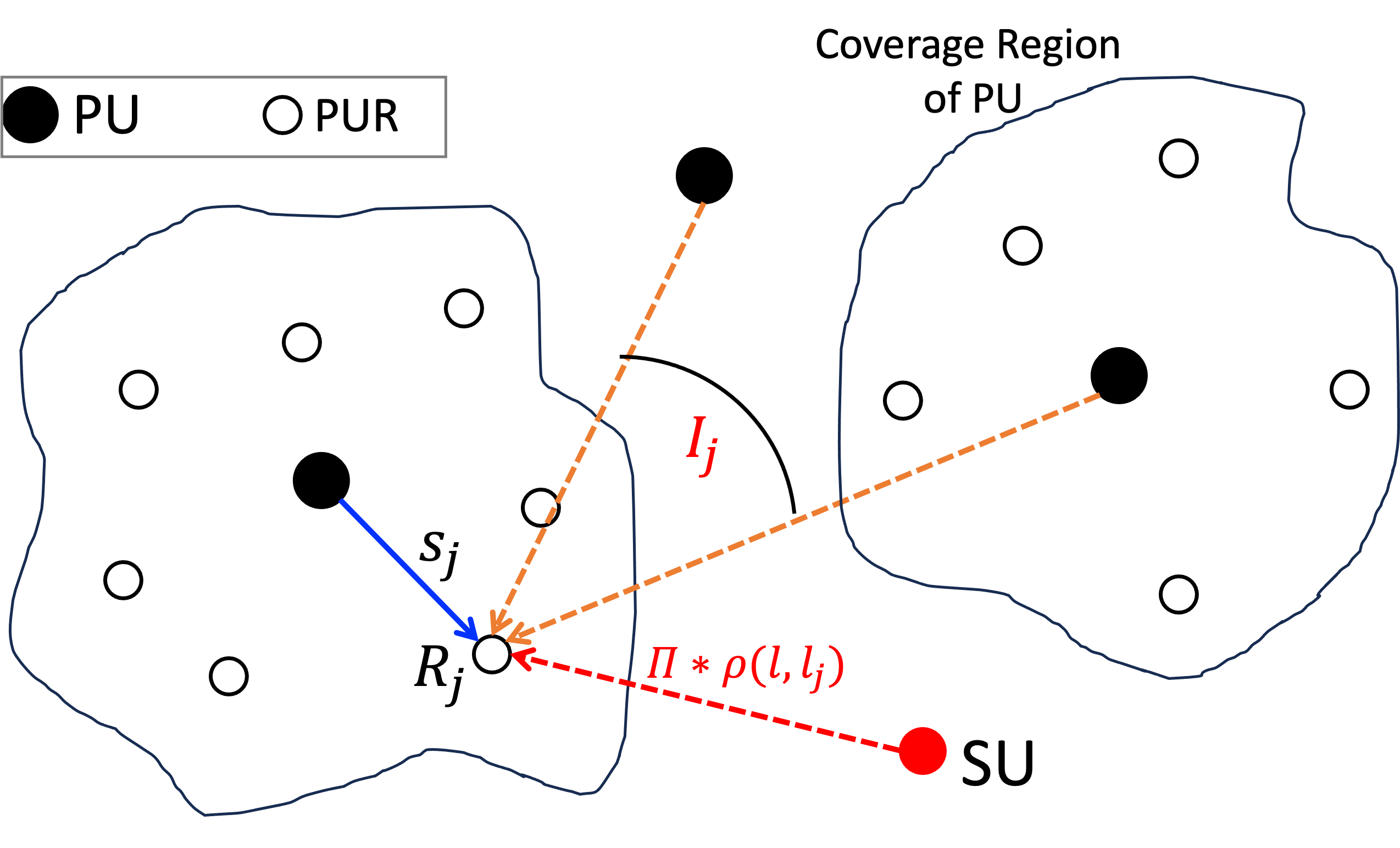
PU Receivers (PURs). A way of modeling the intended receivers of a PU could be to define a coverage region around PU wherein we wish to guarantee reception (see Fig. 1). In this work, as in [22, 25], we model the intended receivers of a PU as a finite set of receiver nodes, which we denote as PURs. The PUR model is without loss of generality since, in general, the PURs can be distributed arbitrarily around a PU. The PUR model is also more computationally efficient than the coverage-region model in determining whether an SU’s transmission causes harmful interference to PU’s receivers. Later, we assume that the distribution method for PURs is “similar” across all PUs, to obviate the need to represent them explicitly in the SA’s input image (see §III-A for more details).

Spectrum Allocation Objective: SU Transmission Power. The general spectrum allocation problem is to allocate optimal power to an SU’s request across spatial, frequency and temporal domains. We focus on the core function approximation problem, which is to determine the optimal power allocation to an SU for a given location, channel and time instant—since frequency and temporal domains are essentially “orthogonal” dimensions of the problem and thus can be easily handled independently (as done in §III-F). We thus assume a single channel and instant for now, and discuss multiple channels and request duration in §III-F.

Determining Optimal Power Allocation. Consider a shared spectrum area with PUs deployed, and an SU request for transmission from a given location $l$. If the PUs information and the path-loss function are known, then the optimal power that can be allocated to SU without causing harmful interference to PUs can be computed as follows [16, 17, 22]. Let us denote the path loss function between a pair of given locations by $\rho\left(,\right)$; thus, a signal transmitted at power $t_{i}$ from location $l_{i}$ yields a received power of $t_{i}\cdot\rho\left(l_{i},l_{j}\right)$ at location $l_{j}$. Let the total interference from other PUs plus noise at $R_{j}$ be $I_{j}$. To ensure that the signal-to-noise ratio at each $R_{j}$ is more than a desired value, say $\beta$, the maximum power $\Pi$ that can be allocated to the SU is:

$$\Pi\leq\min_{j}\frac{(s_{j}/\beta)-I_{j}}{\rho(l,l_{j})},$$ (1)

where $s_{j}=t_{i}\rho(l_{i},l_{j})$ is the signal strength received at $R_{j}$ from its PU transmitting at power $t_{i}$ from location $l_{i}$. See Fig. 1. Note that the above formulation is largely without loss of generality— as the path-loss function $\rho$ can be arbitrary. Irrespective, the fundamental techniques developed in our work are largely independent of the formulation or algorithm used to determine the optimal allocation power—since learning models and techniques are solely based on training examples. In §IV, we use the above formulation to generate the training examples used to train the models.

Two Settings: PU-Setting and SS-Setting The above formulation requires knowledge of PUs information as well as the path-loss functions. However, in most settings, neither of them may be available; in fact, this is one of the key motivations of our learning approach. In particular, PU parameters may not be available in military or government setting, e.g., in the CBRS 3.5GHz shared band [1] wherein the licensed users include Navy radar systems. In light of above, we consider two different settings in this paper, based on the availability of PU information/parameters.

PU-Setting. In this setting, the PUs’ parameters are available—for determination of spectrum allocation. A PU’s parameters include its location, transmit power, and its PURs’ locations.

SS-Setting. In this setting, PUs’ parameters may not be available, e.g., in military or government settings. In this case, to determine spectrum allocation, we make use of a crowdsourced sensing architecture where relatively low-cost spectrum sensors (SS) are deployed with a high granularity [12, 10, 24, 39]. In such a crowdsourced sensing architecture, allocation decision is based on SS parameters, which includes for each sensor its location and received (aggregated) signal strength from the PUs (which presumably is representative of the PUs parameters). Allocation based on SSs parameters is implicitly based on real-time channel conditions, which is important for accurate and optimized spectrum allocation as the conditions affecting signal attenuation (e.g., air, rain, vehicular traffic) may change over time.

II-A Related Work

The spectrum allocation problem has been studied extensively (see [50, 42, 19] for survey), especially in the context of shared spectrum systems. In a centralized SM architecture, it is generally assumed that the SM has complete knowledge of the PU parameters. Many prior works also assume a propagation model which, in conjunction with known PU parameters, allows spectrum allocation power to be computed via linear programming [42] or other simple techniques for common optimization objectives. However, in practice, PU parameters may not be available, e.g., in the CBRS (3550-3700 MHs, in the 3.5GHz) band [1] wherein the licensed users include Navy radar systems. As most propagation models have unsatisfactory accuracy, spectrum allocation must be done overly conservatively for correctness. In particular, in TV white spaces spectrum (54-698 MHz) [2], spectrum allocation is done based on a database with TV channel availability at each location; in essence, the SU is allowed to transmit with a certain power, if the signal received at its location is below a low threshold. Such a listen-before-talk [29, 41] allocation strategy in general can be very conservative due to a combination of reasons: (i) the observed signal is actually an aggregate over all PUs in the same band, (ii) path-loss need not be symmetric, (iii) SUs may want to transmit at a much lower power than the PUs, and (iv) PURs may be a distance away from the PUs. In static systems, a database approach [1] can also be used by pre-computing the SA function and storing in the databases; however, such an approach doesn’t work in any dynamic situation, e.g., SUs in tertiary level, PUs changing powers, path-loss changes due to real-time conditions. In a closely related work,  [22] has developed an interpolation-based spectrum allocation scheme that works by first estimating the desired path-loss values based on signal strength readings from deployed spectrum sensors. In particular, they use inverse-distance weighted and Ordinary Kriging interpolation schemes to estimate the path-loss values. We compare our approach with theirs in §IV-§V.

Machine Learning (ML) Based Approaches. To the best of our knowledge, there have been no prior works that have used supervised learning to directly learn the SA function, especially as defined here. The closest work is [5] which uses supervised learning to analyze spectrum occupancy based on the sensed signal at the SU. There have been some works [43] on learning the path-loss function, which can then be used to allocate spectrum using Eqn. 1. However, Eqn. 1 requires knowledge of PU parameters, which may not be available. Moreover, the path-loss function fundamentally encodes more information than the SA function, and thus, would likely require much more training.

Reinforcement Learning (RL) Approaches. Reinforcement learning (RL) models have been used in slightly different spectrum allocation settings wherein multiple agents are involved or competing with each other for spectrum resource and they undertake a sequence of actions. E.g., [33, 21, 49, 36, 14] have applied RL techniques for power control in multi-agent cellular networks, wherein the agents interact with each other and cell towers to determine power allocation. In addition, RL-based spectrum allocation works in radio networks (see [34, 46] for surveys) have largely focused on channel assignment; in contrast, our work is focused on power allocation. Zhang et al. [48] propose a deep RL algorithm where a deep neural network is used to help SUs obtain information about PUs’ power policies.

Multiple Channels and Other Objectives. In this paper, we implicitly assume a single channel for the most part. Spectrum allocation for multiple channels can be done by using single-channel techniques independently for each channel and then selecting one of the available channels based on some criteria (see §III-F). For example, H. Wang et al. [44] picks a channel that maximizes the aggregate data rate of SUs, and X. Li et al. [30] picks a channel that allows for minimum transmission power for a desired SU data rate. Other works have addressed spectrum allocation with other optimization objectives. e.g., researchers have considered throughput maximization as an objective [37, 45] under various constraints such as maximum allocated power [30], given QoS requirements [28], etc. Fairness and energy efficiency are some other criteria considered [47, 9, 20].

II-B Our Learning Approach

Motivation for Learning SA Function. Our goal is to allocate spectrum efficiently to SUs in general settings, e.g., when PU parameters may not be available. To motivate and justify our learning based approach, we make the following remarks. First, we note that to allocate spectrum near-optimally to secondary users in general scenarios, we fundamentally need to have knowledge of the signal path-loss function. In practice, however, even the best known path-loss models [13, 32] have unsatisfactory accuracy, and conducting extensive surveys to gather path-loss values is infeasible and moreover, may not even reflect real-time channel conditions. In absence of knowledge of a path-loss function, to allocate spectrum efficiently, we propose to just learn the spectrum allocation function directly using supervised learning techniques. Second, in our context, an unsupervised approach is meaningless as unlabelled samples have minimal information (actually, zero information in the PU-Setting), and as explained in §III, a reinforcement-learning approach is also not suitable for our setting. Third, learning the path-loss function first and then using Eqn. 1 to allocate spectrum is certainly a feasible approach – but, since the path-loss function fundamentally encodes more information than the SA function, it would likely require much more training (note that the SA function depends only on the most restrictive of the PURs). Finally, non-trivial parameters such as weather, terrain and obstacles, PU transmitters being directional, etc., can be relatively easily incorporated in a learning approach (see §III-F), while they would require more sophisticated modelling techniques and algorithms to be incorporated in non-learning approaches.

Based on the above observations and insights, we propose to learn the SA function directly from training examples. In general, our goal is to learn the SA function accurately with minimal training. Below, we discuss the inputs/features to our learning models, and the gathering/generation of training samples.

Inputs/Features of the SA Function $\mathcal{A}$. For most of the discussion in this paper, we focus on spectrum allocation to a single/first SU in a given area; multiple or subsequent SUs can be handled similarly as discussed later in §III-F. In the simplest of settings, the PUs’ information/parameters (location and transmit power) do not change over time, in which case the SA function can be simply represented as a function of just the SU’s location, as the fixed PU parameters will be automatically captured within the learned model. In this work, we focus on the more general settings wherein the PUs’ information (location and power) may change across training and evaluation samples. For our two settings, viz., PU-Setting and SS-Setting, inputs/features of our SA function are as follows.

1. PU-Setting. In this setting, the PUs’ parameters are available for spectrum allocation determination. Here, the inputs to the SA function are PU parameters $\mathcal{R}$ and location $l$ of the requesting SU, and thus, the SA function can be represented as a real-value function $\mathcal{A}(\mathcal{R},l)$.

2. SS-Setting. In this setting, PUs’ parameters may not be available, and, as mentioned before, we use spectrum sensors (SSs) to gather received power and use sensors’ readings to determine spectrum power allocation. Here, the inputs to the SA function are (i) SSs parameters $\mathcal{S}$, and (ii) location $l$ of the requesting SU. Thus, the SA function is can be represented as $\mathcal{A}(\mathcal{S},l)$. For each SS, its parameters may include its location and aggregate received power from the PUs, and in general, may also include the mean and variance of the Gaussian distribution of the received power.

Gathering and Labeling Training Samples. Note that gathering a training sample for $\mathcal{A}$ entails gathering feature values and determining its “label”—in our context, for a given feature vector (SU location and PUs/SSs parameters), the label is the maximum power that can be allocated to the SU without causing harmful wireless interference at any of the PURs. In the PU-Setting, the features are the available PU parameters. In the SS-Setting, for gathering training samples, we need to deploy SSs and gather received powers (see §V) for collecting sample features. In either setting, to label the sample, we need to estimate the maximum allowable power at a given SU’s location; this entails simulating PURs and determining the maximum SU transmission power that allows PURs to receive the PU signal (i.e., ensures that the signal-to-noise-ratio is above a desired constant). To estimate the maximum SU power allowed, we can do a binary search on SU power, as done in our tested setup described in §V. To circumvent the collection of noisy samples, we can throw out samples that cannot be reproduced. We acknowledge that the training process can incur a substantial cost, but can be automated using drones for entities. More importantly, training is done only one-time, and thus, some amount of training cost is tolerable.

III CNN-based Deep Learning Approach

In this section, we motivate convolutional neural network’s (CNN) suitability for our context, and design an an efficient CNN architecture and associated techniques for our problem.

Motivation for Using CNNs for SA Function. We observe that SA function can be looked upon as image regression function, with the inputs to the SA function (SU location, PUs/SSs parameters, etc.) represented as an image and the regression value representing the optimal allocation power. Framing SA function as an image regression function allows us to leverage known advanced image regression models. In particular, CNNs have been very successful in image classification or regression tasks or in capturing patterns/objects in images, because CNNs are able to exploit the spatial structure in images via use of learnable spatially-localized filters (or kernels) in its convolution layers. In our context, the spatial nature of the SA problem (i.e., entities deployed over a geographic area) means that the input to the SA problem can be represented as a 2D image with sufficient accuracy. Such a input representation allow us to use CNNs to learn the SA function effectively. We corroborate our above intuition about suitability of CNNs to our problem via extensive evaluations in §IV. For the general case of multiple SUs, we augment our CNN model with Recurrent-Neural Networks (RNNs) in §III-F.

Challenges. However, there are significant challenges that need to be addressed, to make CNN a viable and efficient approach to learn the SA function. These include the pre-processing of samples into ”images” to feed as input to a CNN model, creating an efficient CNN architecture, ensuring minimal false positives, handling multi-path fading effects, minimizing training cost, etc. We discuss these challenges in the following subsections.

Other Machine Learning Models. We believe that CNNs are best suited to model the (single SU) SA function. However, other machine learning models can also be used to learn the SA function—in particular, we also evaluate neural networks (NNs) and space-vector machines (SVMs) approaches in §IV-A.

However, we note that reinforcement learning (RL) approach is not suitable for learning the spectrum power allocation function, as defined in this work, for the following reason. Learning our SA function is fundamentally a supervised learning problem—since our learning goal is to approximate a function using labeled training examples (which can be gathered, as discussed before). In contrast, in RL settings, an agent learns a policy about which action to take on each state so as to maximize the cumulative reward; the learning of such a policy is driven by (i) the rewards given by the environment based on the current/next state(s) and/or the action taken, and (ii) the Markov-decision process (MDP) over the system states and actions that represents how the system transitions through states potentially influenced by actions. As there is no underlying MDP governing our spectrum allocation setting, the RL approach is not suitable to our context.

III-A SH-Alloc: Shallow CNN Model

In this subsection, we discuss our basic CNN architecture and approach, which we refer to as SH-Alloc, as it has a small number of layers. In the next subsection, we will extend this approach to the DeepAlloc approach that uses a much deeper CNN architecture with a larger number of layers. We start with discussing our strategy to pre-process training samples into images.

Pre-Processing Training Samples to Images. The first challenge in applying CNNs to our context effectively is to transform each training sample to an “image” for input to the CNN model, in a way that it is most conducive to efficient learning. Representing the entities (PUs, SSs, SUs) as objects in a 2D image is a natural choice. In particular, we could represent each entity type with a different color or shape, or more specifically, represent each entity by a disk of a certain color with a radius based on the transmit/received power. Our choice of image representation is tantamount to feature engineering [6], and can have a significant impact on the training cost. Below, we discuss the choice made in our model design. First, we assume that the PURs are distributed similarly across all PUs; more formally, we assume that the distribution of PURs around its PU $P$ is a function of $P$’s parameters (location and power). Under the above assumption, we do not need to represent PURs of any PU in the input image—as the distribution of PURs can be learned by the model from each PU’s parameters. E.g., if for each PU $P$, its PURs are distributed uniformly within a fixed radius around $P$ (or within a radius proportional to $P$’s power), then we don’t need to represent PURs in the input image.

Figure 2: Image representation of a sample for input to the DeepAlloc model. Here, there are four PUs (2 in the first sheet, and 1 in the other two sheets) and one SU (in the fourth sheet). Each sheet for the PUs corresponds to a range of PU’s transmit power; e.g., PUs whose transmit power is in the range -10 to 0 dBm are placed in the first sheet. When representing SSs in SS-Setting, we place SSs in the sheets based on their locations.

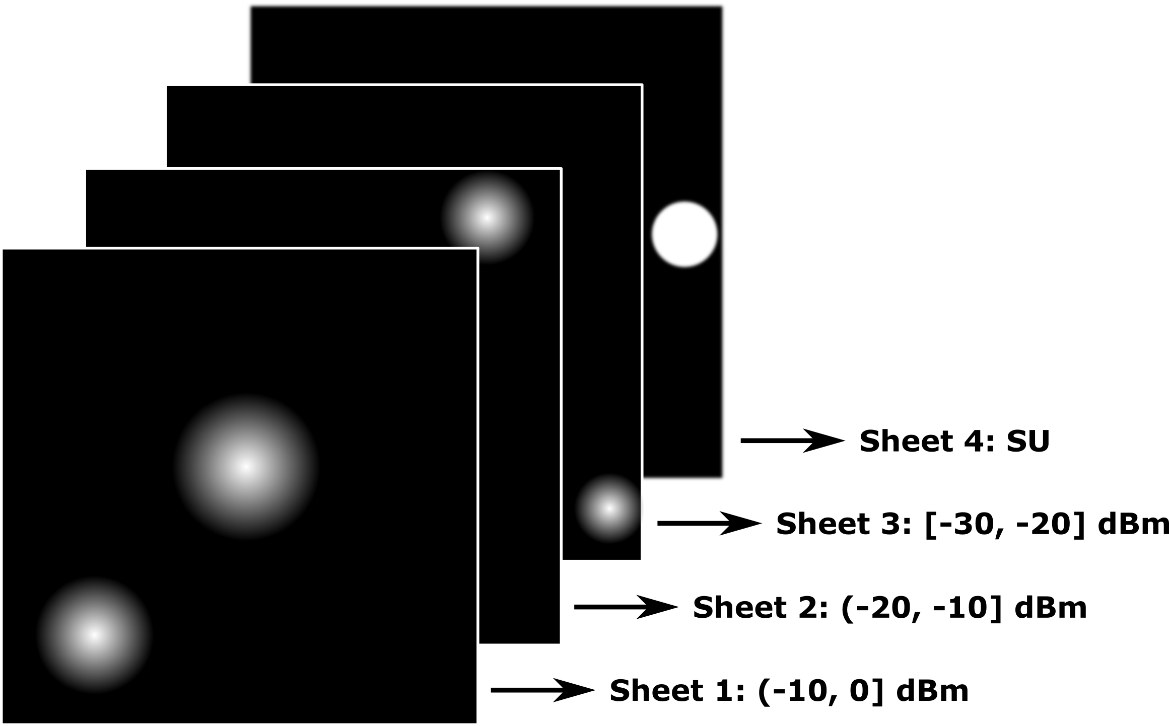
PU-Setting: Representing PUs in Multiple Image “Sheets.” Note that just using shapes or colors for different entities is not sufficient, as we also need to represent transmit/received powers. Just using radius to represent powers is not viable either, as we may start getting intersections between shapes. Thus, we compose the input image of a certain number of “sheets” (see Figure 2). Then, we divide the expected transmit-power range into ranges of about 5-10dBm, and assign each PU to the appropriate image sheet depending on its transmit power. Within each sheet, we then use disks to represent each PU, with the brightness of the center pixel as well as the radius of disk proportional to the transmit power. In addition, to give more importance to the center (which represents the true location) and to suggest signal attenuation away from the center, we decrease the brightness of the pixels away from the center in a logarithmic manner. If there is an intersection between two objects in the same sheet, we aggregate the intensity of the common pixels. Unlike normal images which are composed of three sheets corresponding to red, green, and blue colors, we may use more than three sheets.

SS-Setting: Representing Spectrum Sensors’ (SSs) Readings. SSs can be represented similar to PUs with the size of their disk proportional to the received (rather than transmit) power. However, unlike PUs, we place SSs among the sheets based on their location rather than received powers, e.g., SSs from certain grids were always placed on the first sheet irrespective of their received-power readings. In our evaluations, we observed that placing SSs over sheets based on locations improved the performance of our models significantly compared to placing the SSs based on received powers.

Representing SUs. We use a separate sheet to represent SU(s), instead of representing them with a different shape/color, to facilitate potentially more efficient training.

SH-Alloc CNN Model Architecture. To design a CNN architecture to learn the SA function efficiently, we need to carefully determine the various model parameters. For our SH-Alloc model, we choose these parameters as follows. (i) Number of convolution layers in a CNN model plays an important role in training cost as well as model accuracy. In general, a deeper model (i.e., with more number of convolution layers) performs better than a shallow one but incurs more training cost. In our context, only a few thousand training samples being feasible to gather, we use 5 convolution layers, and 3 fully-connected layers as in a neural-network architecture. (ii) Filter Size: To be able to ”detect” small-radius PUs of small power values, we use a $3\times 3$ filter in the convolution layers. The number of filters is small for the initial layers, and then increases with the ”depth”; this facilitates the detection of more and more complicated features in the deeper layers. (iii) Activation Function: In our context, as the final output of the model is a real number, we chose a linear activation function for the last network layer with only one neuron. For other layers, we use Rectified Linear Units (ReLU) [35] activation function as its non-linearity enables the model to learn a more complex function faster.

The overall CNN-based spectrum allocation system is shown in Fig. 3, including components discussed in the following subsections.

Figure 3: CNN-based Spectrum Allocation System. For the CNN Model component, SH-Alloc uses a shallow CNN model without any pre-training, while DeepAlloc uses a deep pre-trained CNN model obtained from Fig. 4. In both cases, after any pre-training, the (field) training samples are gathered, converted into images, and then used to (further) train the CNN model. The learned model is then used to allocate spectrum to requesting SUs.

III-B DeepAlloc: Pre-Trained Deep CNN Model

Figure 4: DeepAlloc Pre-Training Process. Here, we generate a large number ($\approx$ 1M) of images assuming a log-normal propagation model based on an estimate path-loss exponent, and pre-train a deep CNN model (we used ResNet) using these generated images. The pre-trained model is then used in Fig. 3 for further training using a smaller number of field training samples.

It is well understood that deeper neural networks, i.e., neural networks with more layers, and in particular, deeper CNN models can yield much better performance with their ability to learn more complex functions, with sufficient training data. However, there are two major challenges with using deep models. First, as the number of layers increase, so does the number of parameters to learn—which in turn requires a much larger number of training samples. Second, a deeper model is more likely to learn a function that overfits the training data, if the training data is not sufficient. The perfect solution is to use a deep network but also have a sufficiently large training set. However, in our context, it is infeasible to gather more than a few thousand samples as the deployment and/or labelling costs are high, while a very deep (e.g., with 20-100 layers) network may require close to a million samples to train properly [40, 23, 15].

Using Pre-Trained Models. Our approach to address the above challenge is to use a pre-trained deep model, i.e., a deep model that has already been trained with readily-available images, which may not represent spectrum allocation samples. Such a strategy has been often used in computer vision applications with great success. Similarly, we could also use pre-trained deep well-known models such as VGG [40], ResNet [23], Xception [15] which have been trained with around 1 million daily-life images, and then train them further with a few thousands of spectrum allocation training samples, as in the previous subsection.

DeepAlloc Approach. One unique aspect of our context is that the pre-training samples or images can be easily synthesized based on an assumed propagation model. Thus, to obtain better performance than the above models pre-trained with daily-life images, we can pre-train a deep architecture (we use ResNet [23]) with generated spectrum allocation images based on an assumed log-normal propagation model with an ”appropriate” path-loss exponent. (Results in Fig. 10(b) of §IV-A validate the above pre-training approach.) The path-loss exponent $\alpha$ can be derived by gathering a few (say 100-200) path-loss samples, and determining the best $\alpha$ that minimizes the error between the actual samples and those from the log-normal model. See Fig. 4. Then, as before, we train such a pre-trained model further with a few thousands of SA training samples as shown in Fig. 3. We refer to this overall approach as DeepAlloc.

III-C Minimizing False Positive Error

Note that we should rarely allocate a power higher than that determined by Eqn. 1, as it would cause harmful interference to some PURs. Ideally, we would like to minimize such cases, which we call false positives, drastically—perhaps, at the cost of higher number of (and/or errors in) the false negative cases. We address this issue by a combination of two strategies. First, we choose the hyper-parameters of the CNN model in a way that minimizes the number of false positives; the methodology here is largely trial and error, due to lack of techniques to systematically search for hyper-parameter values. Second, we use asymmetry in the training loss function as follows. Essentially, we change the training loss function $\textbf{J}(\boldsymbol{\theta})$ such that false positive samples (an SU requests that gets higher power than the maximum) be penalized more drastically than the other requests. More formally, we define the training loss function as:

$$\textbf{J}(\boldsymbol{\theta})=\frac{1}{m}\left(\alpha_{FP}\sum_{\hat{y_{i}}>y_{i}}{\textit{l}(\hat{y_{i}},y_{i},\boldsymbol{\theta})}+\alpha_{FN}\sum_{\hat{y_{i}}\leq y_{i}}{\textit{l}(\hat{y_{i}},y_{i},\boldsymbol{\theta})}\right)$$ (2)

Above, $\alpha_{FP}$ and $\alpha_{FN}$ are coefficient weights for the false positives and false negatives respectively, $y_{i}$ is the ”ground truth”, $\hat{y_{i}}$ is the predicted value, $\boldsymbol{\theta}$ is the internal set of the parameters being learned, and l(.) defines the error for a single sample. To minimize false positives, we can choose a much higher $\alpha_{FP}$ than $\alpha_{FN}$.

Figure 5: (a) Spectrum allocation function, when there is a single PU and a single SU, due to path-loss with shadowing and multi-path fading effects. Note that the path-loss function has a similar trend. The red plot is a conservative spectrum allocation, based on a similar conservative path-loss function. (b) Modifying labels of training samples to drive the model towards learning a simpler and more conservative spectrum allocation function.

III-D Handling Multi-Path Effect

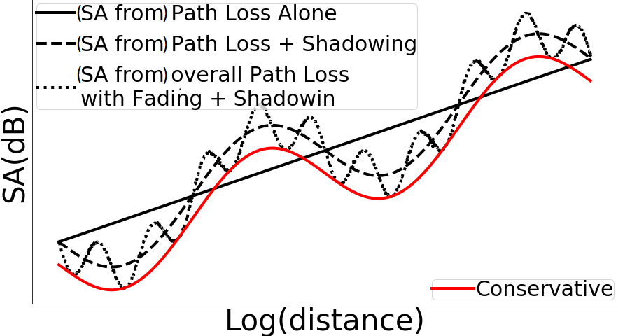
Wireless signal attenuation is a result of three mutually independent, multiplicative propagation phenomena [38], viz., large-scale signal attenuation, medium-scale shadowing, and small-scale multipath fading. The shadowing effect can cause overall path-loss to vary over 10s to 100s of meters, and the fading effect can cause an effect over a few wavelengths. See Fig. 5 (a). The overall effect of these phenomena in our context is that learning the SA function could require a much higher number of training samples—to sufficiently and accurately capture the small to medium scale fluctuations. This challenge is fortunately mitigated by the fact that the small-scale fluctuations in the path-loss function are unlikely to fully manifest in the SA function, as the SA function depends only on the most restrictive of the SU-PUR path losses.

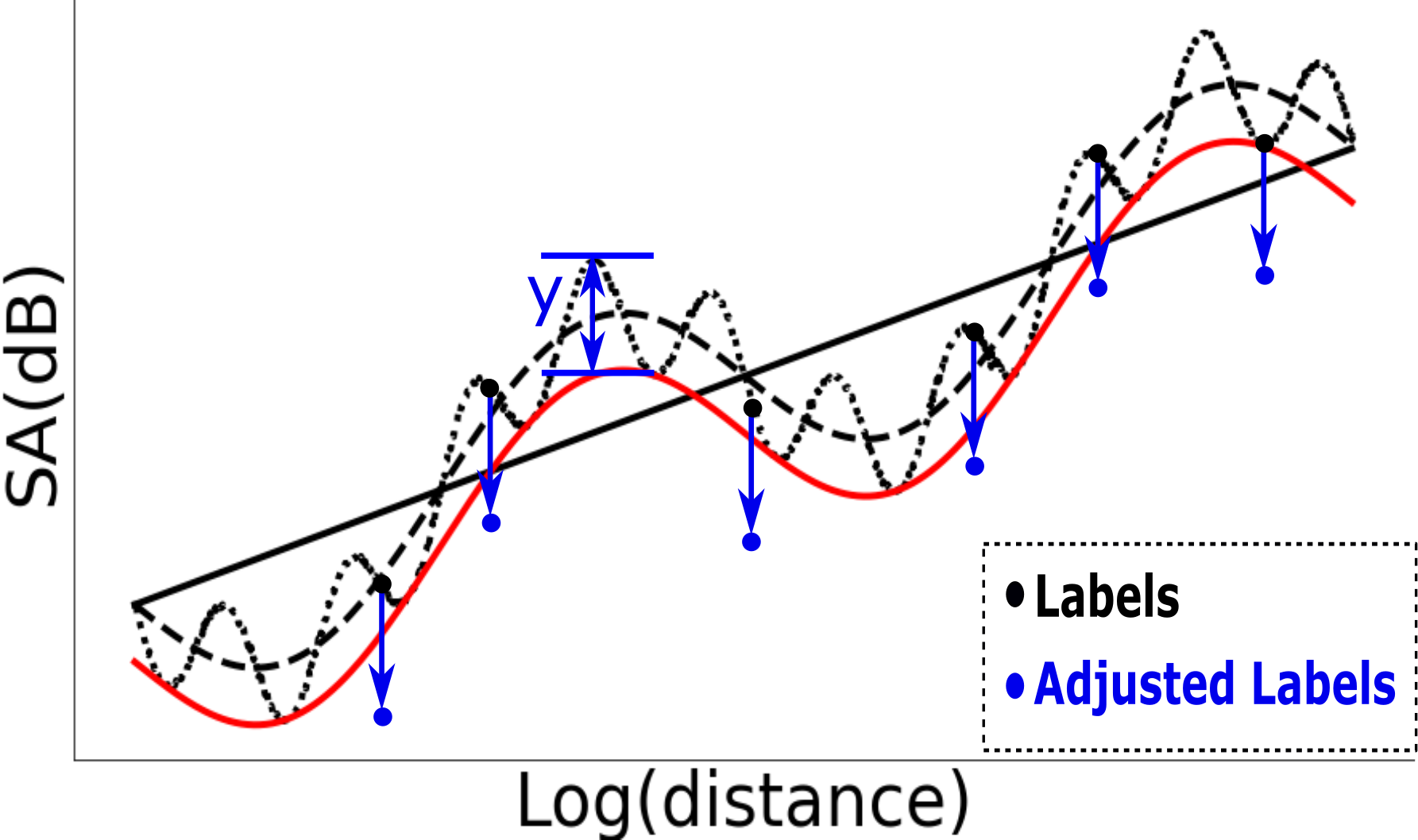
In our context, one way to address the above challenge is to learn instead of a more “conservative” SA function that may be easier to learn but may allocate sub-optimal power. E.g., the conservative SA may be based on a lower-bound approximation of the path-loss function. See the red curve in Fig. 5 (a). We note that the technique in the previous section is also driven towards learning a more conservative function via an appropriate training loss function. However, the model inaccuracy resulting from the multi-path effect is fundamentally due to a lack of sufficient training samples needed to learn a function with high spatial resolution/variability; thus, we can’t fix the model inaccuracy due to the multi-path effect by merely changing the loss function, model, or its training process. Our strategy to learn a more conservative function that addresses the multi-path effect challenge is to actually modify the labels of the training samples appropriately, as discussed below.

Learning a Conservative SA Function by Modifying Training Sample Labels. To ensure few false positives in face of the small-scale multi-path fading effect, we modify the training samples by lowering their labels from the optimal allocated power to smaller values so that the modified training samples represent a ”conservative” spectrum allocation function without the small-scale effects. In particular, let’s consider a training sample–corresponding to a certain set of PUs with given transmit powers, PURs, and SU $\mathrm{S_{i}}$ with allocated power $\Pi$ which satisfies Eqn. 1. (Our discussion in this subsection applies to both settings, viz., PU-Setting and SS-Setting.) Let $l_{i}$ be the location of the SU $\mathrm{S_{i}}$. Now, let PUR $R_{j}$ be the PUR that results in $\mathrm{S_{i}}$’s allocated power, i.e., let $j=\operatorname*{arg\,min}_{j}\frac{\tau_{j}-I_{j}}{\rho(l_{i},l_{j})}$ from Eqn. 1. In the following discussion, we vary $l_{i}$ while keeping everything else constant–thus, we can look at $j$, $R_{j}$ and allocated power $\Pi$ as functions of $l_{i}$. Now, in a sufficiently small neighborhood $N$ of $\mathrm{S_{i}}$, the PUR $R_{j}(l_{i})$ as computed above and thus $\Pi(l_{i})$ must remain fixed for $l_{i}\in N$. Moreover, $\Pi(l_{i})$ is also inversely proportion to $\rho(l_{i},l_{j})$ with $l_{j}$ fixed, and more importantly, variation of $\Pi(l_{i})$ within $N$ is largely dominated by the small-scale effect of the path-loss function. Let $y=\max_{l_{i}\in N}\Pi(l_{i})-\min_{l_{i}\in N}\Pi(l_{i})$, which in some sense is an estimate of the ”amplitude” of the small-scale effect. We now use the value of $y$ to lower the allocated power label of the training samples. See Fig. 5(b). The modified samples essentially correspond to a conservative spectrum allocation function, without the small scale effect. Note that the value $y$ depends on the small-scale effect of the terrain. If we assume the effect to be uniform across the given region, then the same value of $y$ can be used across all the training samples—else, we compute $y$ in each subarea.

III-E Synthetic Samples to Improve Performance

One way to improve performance, i.e., to aid the model in extracting the most information from the given training samples, is to create additional synthetic samples from the training samples. In effect, the new synthetic samples incorporate the domain knowledge used in creating them. In general, from a given sample $\{X,y\}$ where $X$ is the set of features (PU parameters or SS readings, and the requesting SU’s location) and $y$ is the label (allocated power), we create synthetic samples of the type $\{X^{\prime},y\}$ where $X^{\prime}$ is another set of features that yields (approximately) the same label $y$. Below, we discuss the generation of synthetic samples for our two settings, and evaluate the improvement from these strategies in §IV-A.

PU-Setting. Consider a sample $\{X,y\}$ where $X$ includes the PU parameters. For this sample, let $P$ be the PU for the PUR $R_{j}$ that determines the SU’s optimal power allocation, as in previous subsection. Let $\mathcal{P}$ be a set of PUs that are sufficiently far away from $P$. Note that $P$ is determined when labeling the given sample, and $\mathcal{P}$ can be determined from $P$ and the available PU parameters. Now, note that decreasing the power of PUs in $\mathcal{P}$ should not change the optimal power allocated to SU. Thus, we can create additional synthetic samples by considering $X^{\prime}$ which differs from $X$ in that the transmit powers of PUs in $\mathcal{P}$ is lower than that in $X$.

SS-Setting. In the setting, wherein the features are composed of sensor readings, we generate synthetic samples by determining sensor readings at additional locations via interpolation techniques. In particular, based on the log-distance like behavior of signal attenuation, we use a slight modification of the traditional IDW technique. More formally, for a known set of sensor readings $(p_{i},l_{i})$ where $p_{i}$ is the received power at location $l_{i}$, the interpolated value $q$ at a new location $l$ is given by: $q=\frac{\sum_{i}w_{i}p_{i}}{\sum_{i}w_{i}}$, where $w_{i}$ is the weight defined as $w_{i}=\frac{1}{\log_{10}(d(l_{i},l))}$. Based on the above interpolation scheme, for a given sample $(X,y)$ where $X$ is the set of real sensor readings, we can created synthetic samples of the type $(X^{\prime},y)$ where $X^{\prime}$ consists of some readings from $X$ and some interpolated readings.

Rotated Images. In addition to above, we also synthesize additional samples by just ”rotating” the images of the original samples; such a strategy is bound to be useful in regions where the propagation model is largely dependent on the distance. In our evaluations, we rotate the given images by 90 or 180 degrees.

III-F Multiple SUs

Till now, we have only considered spectrum allocation to the initial single SU. Handling subsequent SUs in the same manner as the initial SU above requires allocated power to the active SUs. We start with discussing how to handle multiple SUs one at a time, and then discuss handling multiple SUs simultaneously.

Handling SUs One at a Time. To handle subsequent SUs, we can augment the list of features to include the active SUs’ parameters, and train the model accordingly. This approach is viable, especially in the context of our DeepAlloc model, since active SUs with their parameters (location and allocated power) can easily be represented in the single input sheet dedicated to SUs. The only change we need to make is that we must now represent SU’s allocated power too; we can represent them with a disk similar to PUs, i.e., with the center’s brightness and radius proportional to the allocated power. If multiple SU requests arrive together, then to use the above approach, we need to decide on an order in which to handle the requests. One approach is to handle them in a greedy order as follows; we call this approach DeepAlloc-Greedy. We divide the whole area into non-overlapping subareas, and assign each subarea $X$ a weighted score equal to the total aggregated power transmitting from all the PUs and active SUs in $X$ or its adjoining cells. Then, we pick the SU requests in the ascending order of the weight of the subarea they belong to.

Figure 6: RNN-based Architecture for Simultaneous Allocation to Concurrent SUs. The input to the encoder is the convolution output $F_{i}$ of DeepAlloc for each SU $S_{i}$, and the output of the model is the SU power allocations $\{Q_{i}\}$. The input to DeepAlloc for each $S_{i}$ is a set of sheets representing $S_{i}$’s location $l_{i}$ and independent power $P_{i}$ and PUs/SSs information.

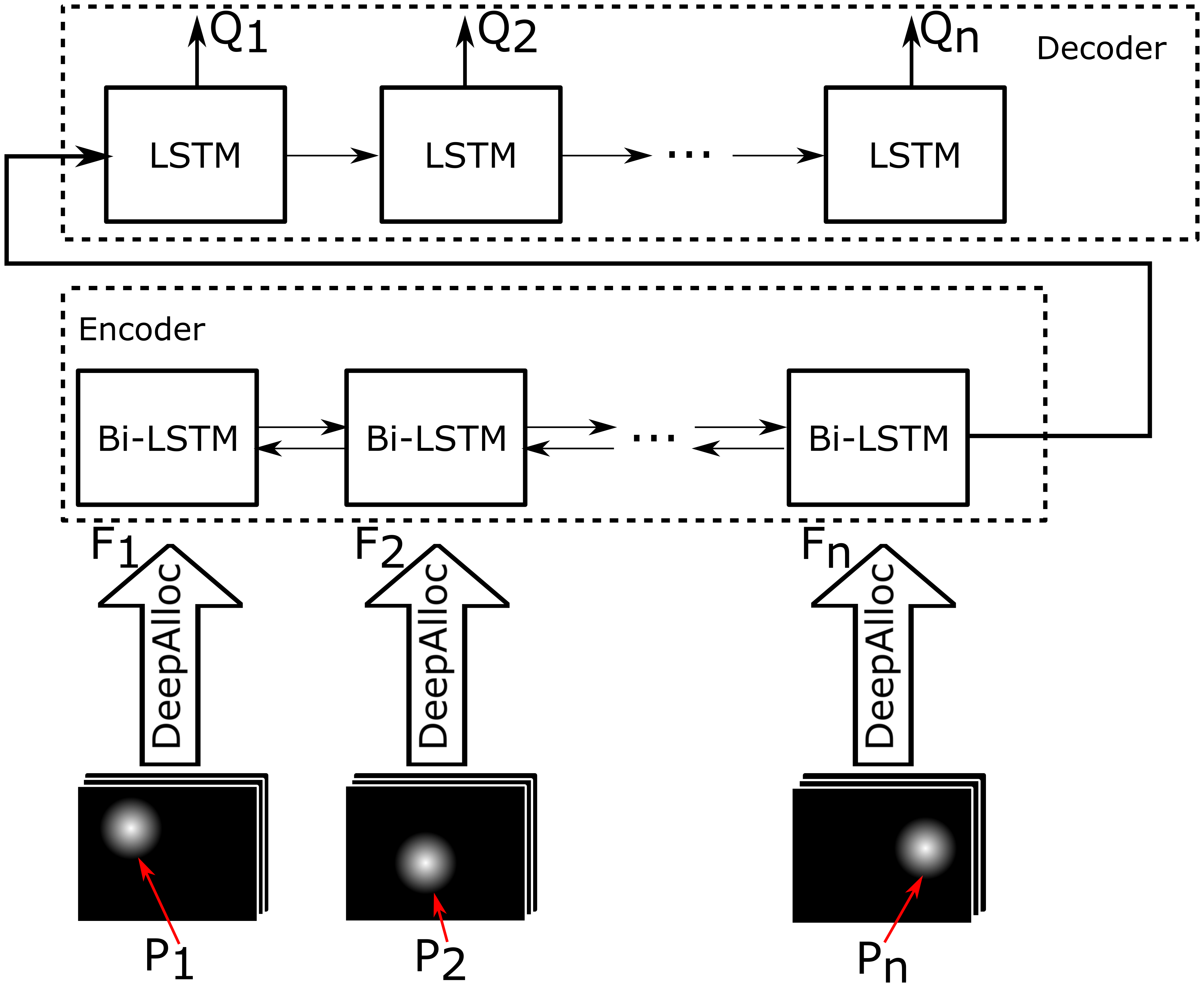
Handling Multiple SUs Simultaneously. Handling SUs one-at-a-time, though easier and simpler, can lead to unfair and/or far-from-optimal (in terms of say, total power allocated) allocation. Thus, we now discuss how to extend our deep-learning models to facilitate simultaneous allocation of powers to multiple SUs. Recall that our DeepAlloc model is trained to predict the maximum power that can be allocated to a single SU. To allocate powers to multiple SUs $\{S_{1},S_{2},\ldots,S_{n}\}$ simultaneously, we need to essentially learn a function that maps the list of SUs’ locations $\langle l_{1},l_{2},\ldots,l_{n}\rangle$ to the list of simultaneous allocated powers $\langle Q_{1},Q_{2},\ldots,Q_{n}\rangle$. To learn the above function, we use two different learning approaches.

(1) DeepAlloc-NN. The simplest approach is to use a traditional neural-network (NN), with inputs as the list of SUs’ locations $\langle l_{1},l_{2},\ldots,l_{n}\rangle$ and other available PU or SS parameters, and the output as the list of allocated simultaneous powers $\langle Q_{1},Q_{2},\ldots,Q_{n}\rangle$. To leverage our developed single-SU model DeepAlloc and facilitate more efficient training, instead of passing the PU or SS parameters, we pass the set of “independently allocated” powers $\{P_{1},P_{2},\ldots,P_{n}\}$ where $P_{i}$ is the power allocated to $S_{i}$ assuming no other SU $S_{j}(j\neq i)$ is active. Thus, the input to the NN is the list $\langle(P_{1},l_{1}),(P_{2},l_{2}),\ldots,(P_{n},l_{n})\rangle$, with the output being the list of simultaneous power allocations $\langle Q_{1},Q_{2},\ldots,Q_{n}\rangle$. The NN is trained using training samples with labels determined as described below. In our simulations, we used a 4-layer NN with 128 neurons in each layer and a dropout of 80% before the last layer.

(2) DeepAlloc-RNN. As mentioned above, we need to learn a model that maps a list/sequence of SUs’ locations to a list/sequence of allocated powers. In recent years, the Seq2Seq models have achieved a lot of success in learning tasks that involving mapping a sequence of words to another sequence of words, e.g, in machine translation, text summarization, image captioning, etc. In particular, Google Translate uses Seq2Seq model to translate a paragraph from one language to another. The Seq2Seq model comprises of an encoder to encode the input sequence, and a decoder to map the encoded data to a target sequence. The encoder essentially creates a sequence of hidden state vectors each of which depends upon the previous input and state vector. Similarly, the decoder uses the created hidden state vectors with appropriate attention/weighting schemes to generate a target sequence.

As our multi-SU spectrum allocation problem entails mapping a sequence of SUs’ information to SUs’ power allocations, we develop a Seq2Seq model with appropriate inputs, outputs, and internal components as follows. For our purposes, we propose to use an RNN-based Seq2Seq model, which we call DeepAlloc-RNN. In particular, we implement the encoder using a bi-directional long short-term memory (LSTM) model and the decoder as a uni-directional LSTM. See Fig. 6. We use bi-directional LSTM as the encoder to facilitate interpretation of the input set of SUs as unordered to signify simultaneous allocation. In addition, rather than passing $\langle(P_{1},l_{1}),(P_{2},l_{2}),\ldots,(P_{n},l_{n})\rangle$ as the input to the RNN model as we did in the above NN approach, we pass the set of feature-sets $\{F_{i}\}$ as input where $F_{i}$ is as follows (see below for the motivation). The feature-set $F_{i}$ (for a given $S_{i}$) is the output of the average-polling layer (Fig. 4) of the DeepAlloc model, when the input (represented in sheets) is SU $S_{i}$’s location $l_{i}$ and independent power $P_{i}$ and given PUs/SSs parameters. See Fig. 6. The above idea of passing $F_{i}$’s to the RNN allows us to encode more information in the input to the RNN, rather than just the power $P_{i}$’s. The final output of the decoder represents the powers allocated to the SUs together.

Determining Training Sample Labels (Binary-Alloc). To train the above models, we need a method to label the training samples; in particular, we need to design an algorithm to determine optimal powers to allocate to multiple concurrent SUs. Our implicit performance metric is the total power allocated to the given set of SUs. Here, in the training phase, even though we can assume knowing whether a certain power allocation to multiple SUs causes interference to any PUR, to determine optimal power allocation to multiple SUs is still non-trivial. Since we couldn’t design an optimal algorithm, we use the following Binary-Alloc heuristic which performed well in practice. The Binary-Alloc heuristic is a binary-search-like iterative algorithm as follows. At any iteration, each SU $i$ is assigned a range $[l_{i},u_{i}]$ of powers such that if all SUs are allocated the lower-end $l_{i}$ of their ranges then there is no interference caused to any of the PURs. The algorithm iteratively reduces (in half) the range of one of the SUs, till the range of each SU is smaller than a a threshold. In particular, in each iteration, the algorithm picks the SU $i$ with the largest range $(u_{i}-l_{i})$, and either moves the lower-bound $l_{i}$ or upper-bound $u_{i}$ to $(u_{i}+l_{i})/2$ depending on whether $(u_{i}+l_{i})/2$ causes interference to a PUR.

Multiple Channels; Request Duration. Till now, we have implicitly assumed a single channel. To handle multiple channels, we can extend our schemes easily. If the signal propagation characteristics are different for different channels, then we can create a separate model for each channel. Then, for a single-SU request, we can pick the channel that allows for maximum power allocation. We can also modify the above multi-SU approaches, for the multi-SU scenario, as follows. The DeepAlloc-Greedy approach extends naturally. For DeepAlloc-NN and DeepAlloc-RNN, we use a simple scheme of uniformly (and randomly) partitioning the given set of SUs into multiple sets and assign a channel to each set; incorporating channel assignment in the model would require much more training, and thus not considered for simplicity. Finally, to handle requests for a specified duration, whenever a currently active SU becomes inactive (i.e., at the end of its authorized duration), we reallocate other active SUs’ allocations.

Other Generalization: Non-Isotropic Users, Weather, Obstacles. We now briefly discuss how our approach can be generalized to handle more general and sophisticated scenarios. We start with discussing how to handle non-isotropic PUs or SUs. In the PU-Setting, the non-isotropic PUs can be represented by an appropriate cone (instead of a disk). In the SS-Setting, the SS readings would naturally incorporate the impact of non-isotropic PUs—and hence, there are no changes to the approach. To handle changes in propagation models due to different weather conditions, we can train different models for different weather conditions (e.g., rainy, summer, winter, etc). To incorporate more fine-grained weather conditions, we can use a separate sheet to represent weather information over the given area. Note that obstacles and terrain information, being largely fixed, is already implicitly incorporated in the learned model.

IV Large-Scale Simulations

In this section, we discuss our large-scale simulation results conducted over a large geographical area (we discuss an outdoor testbed evaluation in the next section). We start with describing the underlying propagation model used in our simulations. All our developed software is open-source [3].

Longley-Rice Propagation Model and Setting. To evaluate our techniques over a realistic propagation model, we use the well-known Longley-Rice  [13] Irregular Terrain With Obstruction Model (ITWOM), which is a complex model of wireless propagation based on many parameters including locations, terrain data, obstructions, soil conditions, etc. We use SPLAT! [31] to generate path-loss values; SPLAT! is an open-source software implementing the Longley-Rice propagation model. When simulating the above propagation model, we consider an area of 1km $\times$ 1km in our state and use the 600 MHz band to generate path losses using SPLAT!. As the height of an entity is an important factor in determining the path loss, we place the transmitters (PU or SU) at a height of 30m and the receivers (PURs and SSs) at 15m above the ground level. For clarity of presentation and due to limited space, in many plots, we only show results for the PU-Setting; in these cases, the observed trend in SS-Setting is similar.

Performance Metrics ($\mathrm{\mathcal{A}_{err}}$, $\mathrm{\mathcal{A}_{fp}}$) and Algorithms. The main performance metric used to evaluate our technique is the average (absolute) difference in power allocated to the requesting SU with respect to an optimal algorithm; here, the optimal algorithm has the knowledge of the exact path-loss values and is thus able to use the Eqn. 1 to compute the power to be allocated to the SU. We denote this measure by $\mathrm{\mathcal{A}_{err}}$. To evaluate the impact of false positives, we also consider the average false-positive error metric $\mathrm{\mathcal{A}_{fp}}$ which is computed as the aggregate error in the false-positive samples over the false positives divided by the total number of samples. The $\mathrm{\mathcal{A}_{fp}}$ metric informally measures the level of interference caused by the spectrum allocations. We implement standard ML techniques, viz., a 3-layered neural network (NN), support vector regression (SVR) [18], our CNN-based approaches SH-Alloc (§III-A) and DeepAlloc (§III-B). Recall that DeepAlloc is based on a pre-trained deep CNN architecture based on ResNet [23] architecture. As detailed in §II, the closest work relevant to our setting is the one in [22] which has available the PUs’ parameter values as well as the SS readings, and uses interpolation techniques to estimate path-loss values between relevant entities; we denote this approach by IP-Based. We note that the simple Listen-Before-Talk approach resulted in a $\mathrm{\mathcal{A}_{err}}$ of a several 10s of dB in our simulations, and has not been shown in the plots for clarity. The large $\mathrm{\mathcal{A}_{err}}$ value for the very conservative Listen-Before-Talk approach (see §II-A) is due to the fact that in a large majority of evaluation samples SU is not allocated any spectrum power as some of the PUs’ power is always received in a large fraction of the area.

Training Samples. As described in §III, there are two types of training samples used in training our models: (i) pre-training samples used to pre-train the DeepAlloc; these samples are based on the log-normal propagation model with an path-exponent computed from a small number of path-loss samples; we computed an exponent of 3.3 from 200 path-loss samples. (ii) training samples, which are gathered in the field as described below; these samples are used to train all the ML models, including the DeepAlloc after pre-training. In addition, for our schemes, we also use synthetic samples (§III-E), which are derived from the training samples. To create a training/evaluation sample, we place 10 to 20 PUs at random locations in the given area and assign them a random power within the range of 0 to -30dBm. Each PU has a random number (5 to 10) of PURs distributed randomly within a distance of 50m from the PU. We vary the number of sensors from 49 to 625 (with 400 as the default) sensors uniformly distributed in the field. For NN and SVR models, we assume the maximum number of PUs to be 20, and use dummy parameter values if the number is less than 20.

Validation and Evaluation Samples. In most of our plots, we vary the total number of training samples from 256 to about 4096 (with a default value of 2048), of which 20% are used for validation purposes (to tune the model’s hyper-parameters) and the remaining are used to train the model. In addition, we create and use 40,000 separate samples for evaluation purposes.

Training CNN models. To pre-train the DeepAlloc using the generated pre-training samples (we used 1m samples), we used SGD optimizer with a mini-batch size of 64. The learning rate starts from 0.01 and is divided by every 10 epochs. We use a weight decay of 0.00001 and a momentum of 0.9. Then, for fine-tuning the DeepAlloc model using real (field) samples, we use Adam [27] optimizer with a very low initial learning rate of 0.00001 while keeping the other parameter values the same. Among all the hyper-parameters, we only optimize the regularization value.

IV-A Performance Results (Single SU)

We now present our performance results for various algorithms and settings. We evaluate various techniques for the case of a single SU request; we consider multiple SUs in the next subsection. Each data point in the plots is an average of over 40,000 evaluation samples.

(a)

(a) PU-Setting.

(b) SS-Setting.

Figure 7: Performance comparison of various schemes for pre-processing the training samples into images.

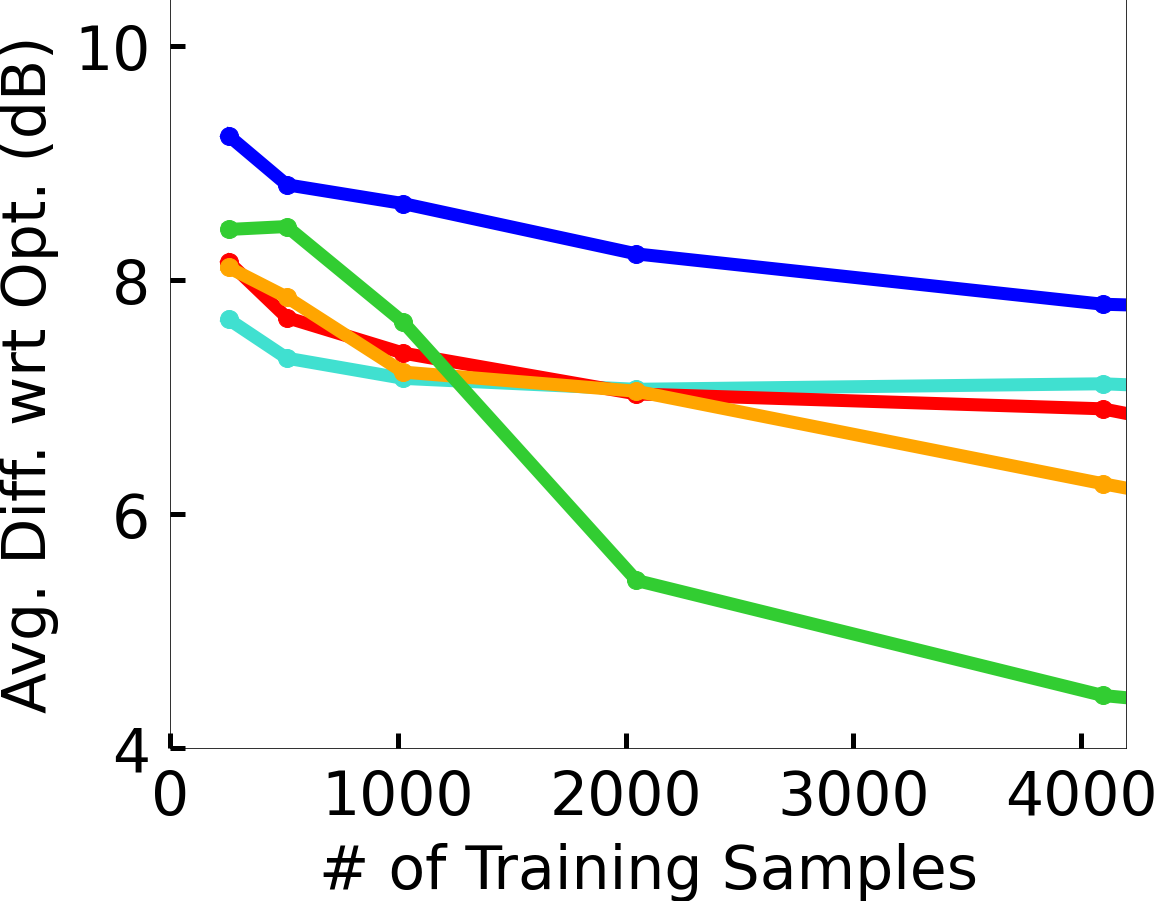
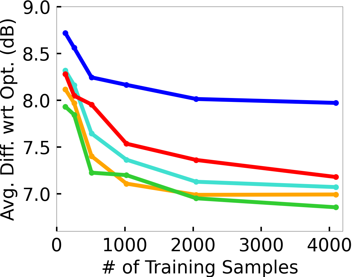
Various Pre-Processing Schemes. We start with evaluating various pre-processing schemes of creating images from the training samples, as input to our basic CNN approach SH-Alloc. Here, we refer to the multi-sheets based approaches (i.e., from Fig. 2) as SH-Alloc-$N$, where $N$ is the number of sheets used for the PUs/SSs. We also evaluate the Colored and Shapes schemes, where the Colored scheme uses different colored-disks (red, green, and blue) for the three entities (PU, SS, and SU) and the Shapes scheme uses a greyscale image with different shapes for the entities (PU: circle, SU: square, SS: rectangle). We maintain the shape sizes to be small (to avoid intersection) and uniform for each entity, but vary the intensity to represent the transmitted (received) power. See Fig. 7 for a performance comparison of the above schemes in both settings. We observe that the SH-Alloc-$N$ schemes outperform the other two schemes, with the increase in $N$ improving the performance as expected. Thus, we use 6 image sheets for PUs/SSs.

(a)

(a) PU-Setting with increasing number of training samples and 10-20 PUs.

(b) PU-Setting with increasing number of PUs and 2k training samples.

(c) SS-Setting with increasing number of training samples and 10-20 PUs.

(d) SS-Setting with increasing number of SSs and 2k training samples..

Figure 8: Performance comparison of various algorithms for increasing number of training samples and PUs/SSs.

(a) Minimizing $\mathrm{\mathcal{A}_{fp}}$.

(b) Handling Multi-Path Effects.

(c) Synthetic samples in PU-Setting.

(d) Synthetic samples in SS-Setting.

Figure 9: (a) Minimizing false-positive error ($\mathrm{\mathcal{A}_{fp}}$), (b) Handing multi-path effect via learning a more conservative function, and (c)-(d) Using synthetic samples to improve performance. Here, (a)-(b) are in PU-Setting; the SS-Setting had similar results.

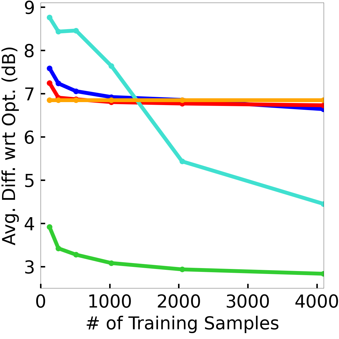
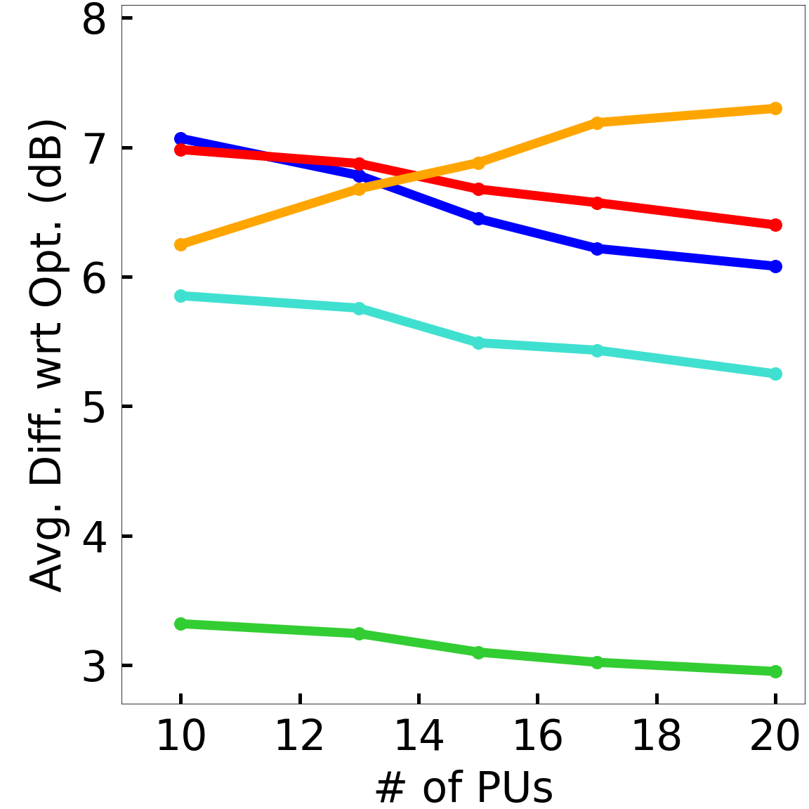
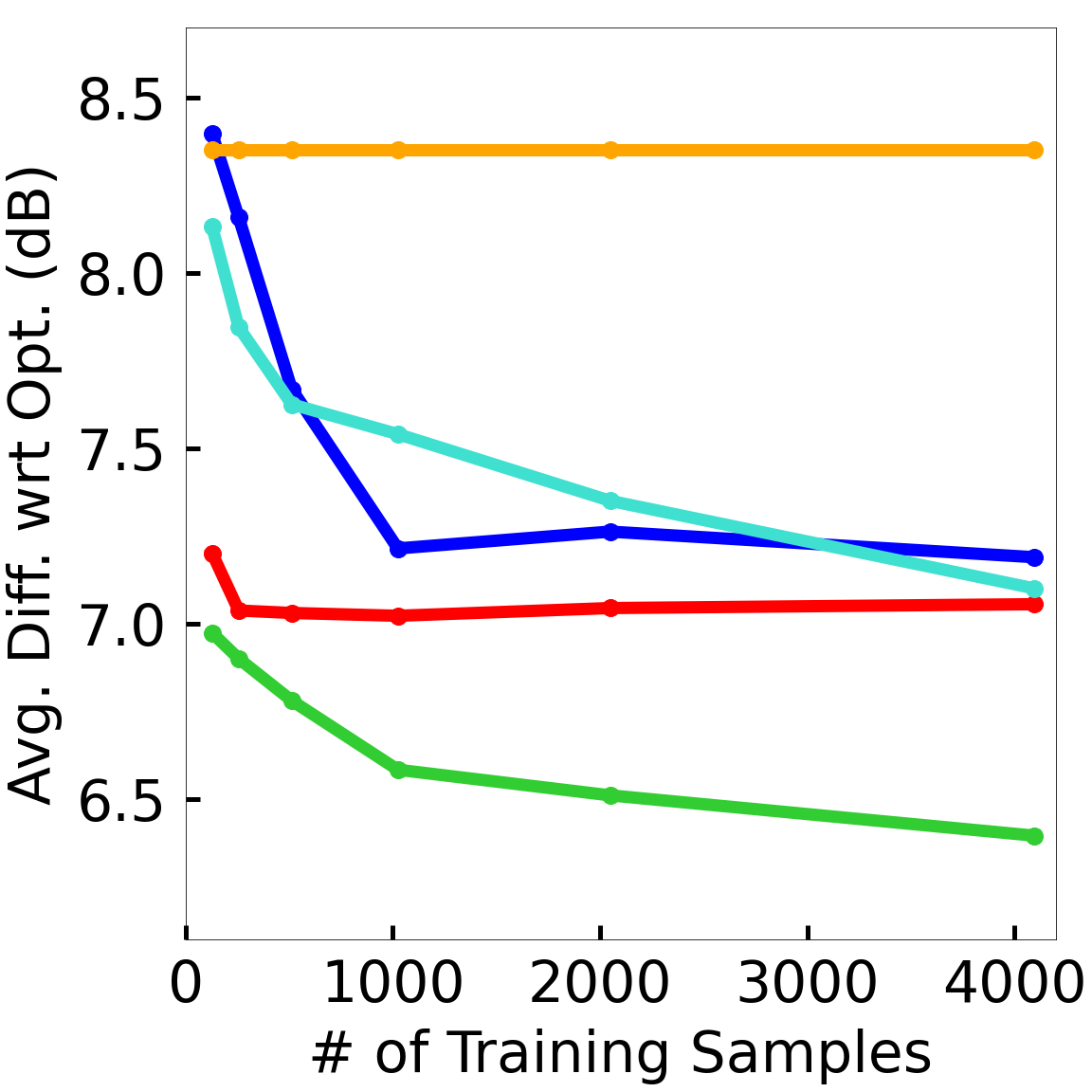
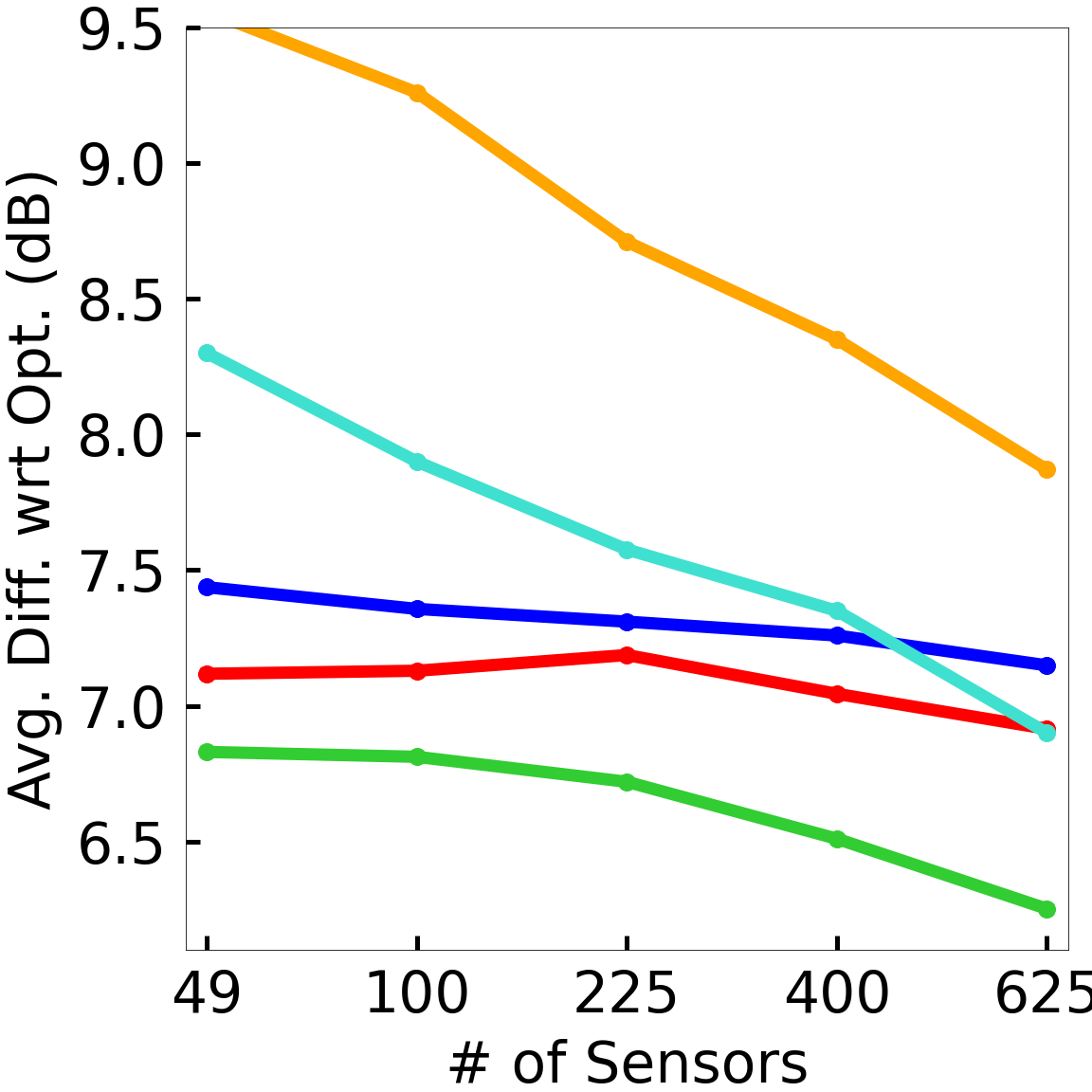
Varying Training Cost and Number of PUs/SSs. We now evaluate the fundamental performance of various algorithms in terms of the key $\mathrm{\mathcal{A}_{err}}$ metric in our two settings, PU-Setting and SS-Setting, for varying number of (field-gathered) training samples and a number of PUs/SSs. See Fig. 8. First, our main DeepAlloc approach outperforms all the other approaches for both settings. More importantly, DeepAlloc delivers great performance for the PU-Setting with less than 3dB performance gap with the optimal solution. As expected, the performance of our approaches is better in PU-Setting than that in SS-Setting, since fundamentally the PU-Setting has more direct information relevant to the spectrum allocation function. Second and more specifically, we observe that both the CNN-based approaches outperform the IP-Based algorithm by a large margin in the PU-Setting; in the SS-Setting, the DeepAlloc approach easily outperforms the IP-Based algorithm, except for large number of sensors wherein both techniques perform similarly. Recall that the IP-Based approach has the advantage of knowing both the PU parameters as well as SS readings, while the ML algorithms have knowledge of only one of these inputs—thus, it is surprising and commendable that DeepAlloc is able to outperform the IP-Based approach. Above observations suggest that DeepAlloc is able to learn the spectrum allocation function effectively. Lastly, we observe that the performance gap between the CNN-based approaches (SH-Alloc and DeepAlloc) is significant—which demonstrates the value of pre-training a deep CNN model.

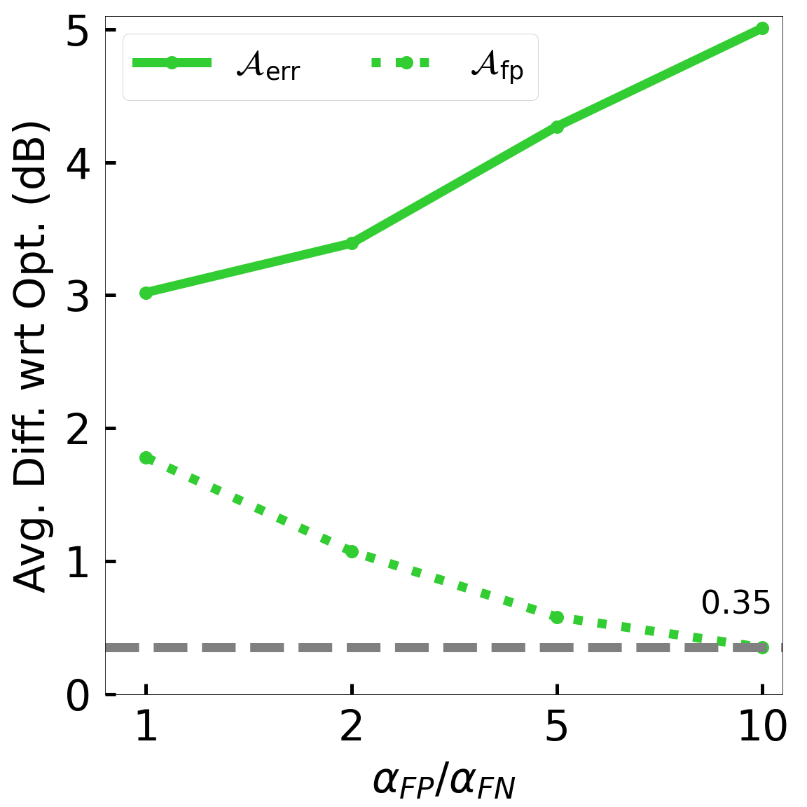
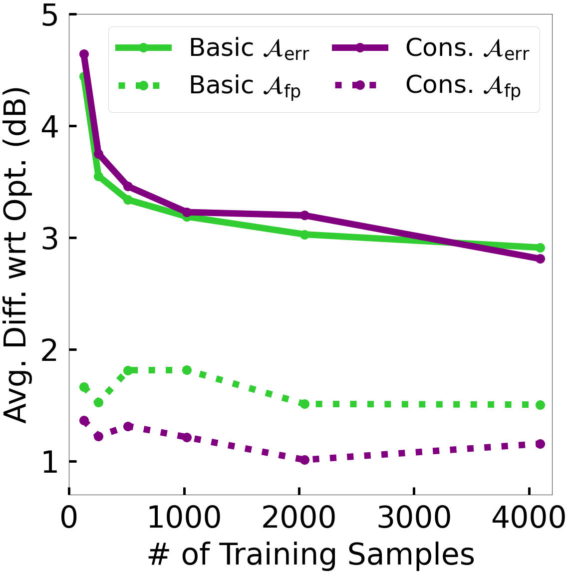
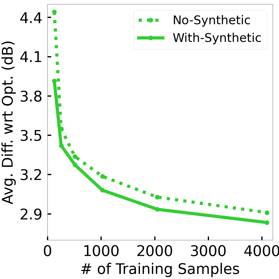
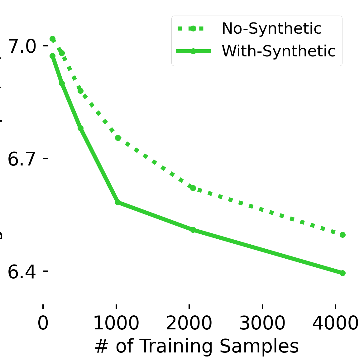
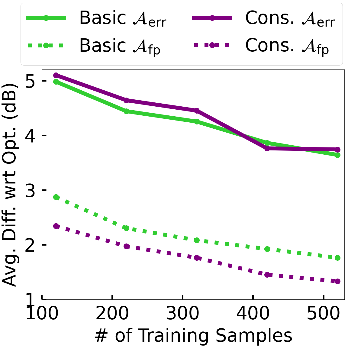
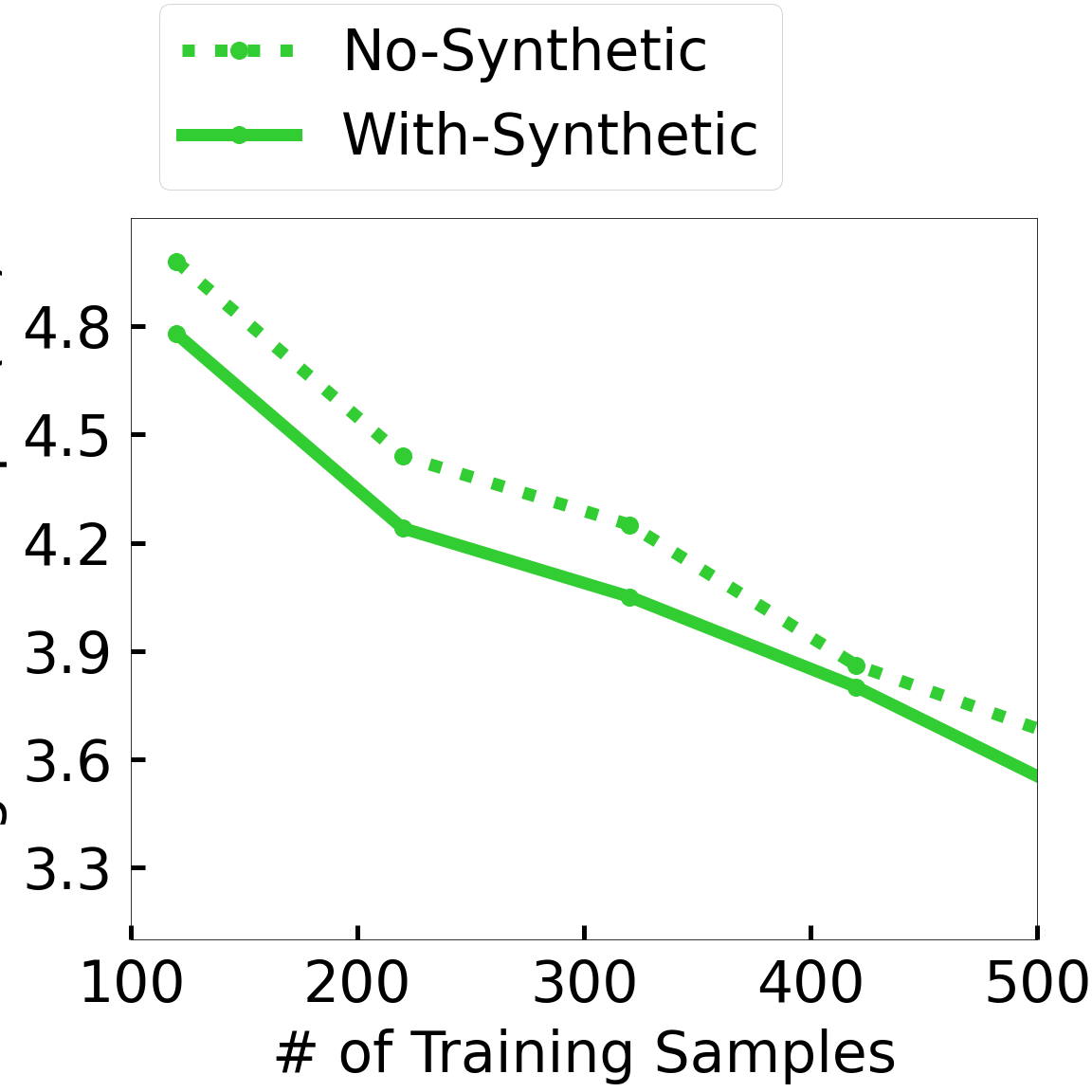
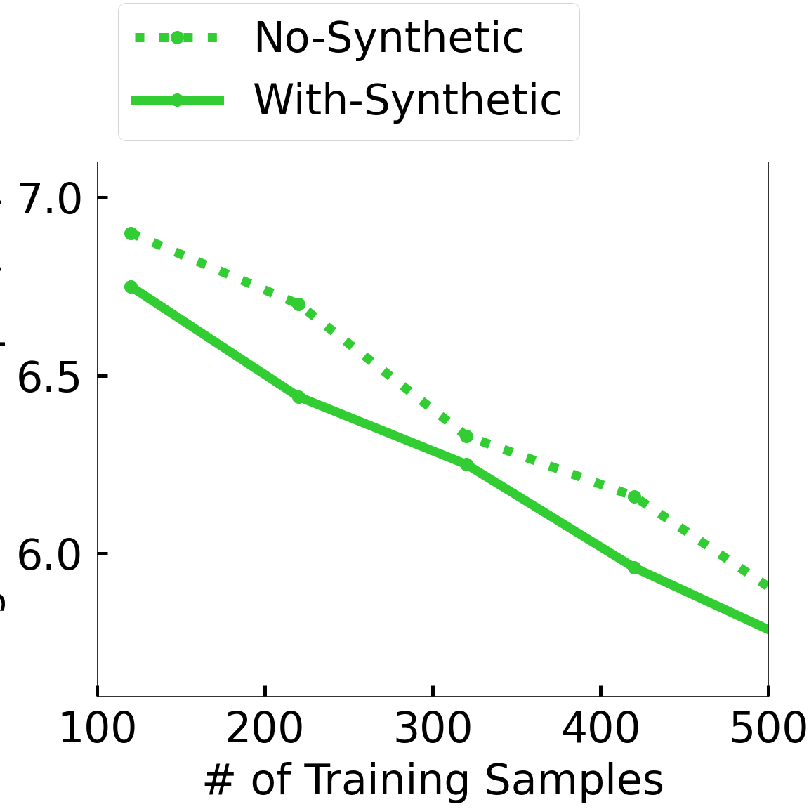
Evaluating Techniques for Minimizing False-Positive Errors, Handing Multi-Path Effect, and Synthetic Samples. We now evaluate our specialized techniques developed in §III-C-III-E for various aspects. See Fig. 9. Fig. 9(a) evaluates the §III-D’s technique to minimize false positives. We plot $\mathrm{\mathcal{A}_{err}}$ and $\mathrm{\mathcal{A}_{fp}}$ metrics for varying $\alpha_{FP}$/$\alpha_{FN}$ ratio; we see that increase in $\alpha_{FP}$/$\alpha_{FN}$ ratio is effective in minimizing the false-positive error $\mathrm{\mathcal{A}_{fp}}$, at the cost of higher average $\mathrm{\mathcal{A}_{err}}$. Next, in Fig. 9(b), we evaluate the technique from §III-D to handle multi-path fading effects by learning a conservative function via modified labels. Here, we plot the $\mathrm{\mathcal{A}_{err}}$ and $\mathrm{\mathcal{A}_{fp}}$ for the basic as well as the conservative technique. We observe that the conservative technique’s false-positive error ($\mathrm{\mathcal{A}_{fp}}$) is indeed reduced without much increase in the total error ($\mathrm{\mathcal{A}_{err}}$), compared to the basic approach. Fig. 9(a)-(b) are in PU-Setting; the SS-Setting results were similar (not shown). Finally, in Fig. 9(c)-(d), we evaluate the benefit of using synthetic samples as described in §III-E. Here, we show PU-Setting as well as SS-Setting as the algorithms for generating synthetic samples are very different. In PU-Setting (Fig. 9(c)), the performance gain due to synthetic samples in positive but minimal—perhaps, because the performance was already near-optimal. In SS-Setting (Fig. 9(d)), we see a significant performance improvement due to synthetic samples—validating our use of interpolation-based synthetic samples. Here, we added 2500 new uniformly-distributed sensors and interpolate their readings using the four nearest original sensors.

(a) Performance across regions.

(b) Various pre-trained CNN models.

Figure 10: Performance comparison of (a) DeepAlloc over different regions, and (b) various pre-trained models for increasing number of training samples.

(a) Last SU’s Allocation.

(b)

(b) Average difference of aggregated SUs power

(c) Fairness across multiple SUs.

(d) Average data rate by multiple SUs.

Figure 11: Multiple SUs. (a) Power allocated to subsequent SUs, in presence of other active SUs. (b)-(d) Average different wrt ground truth (GT), Fairness (max/min ratio), and Total data rate for multiple SUs by various multi-SU algorithms.

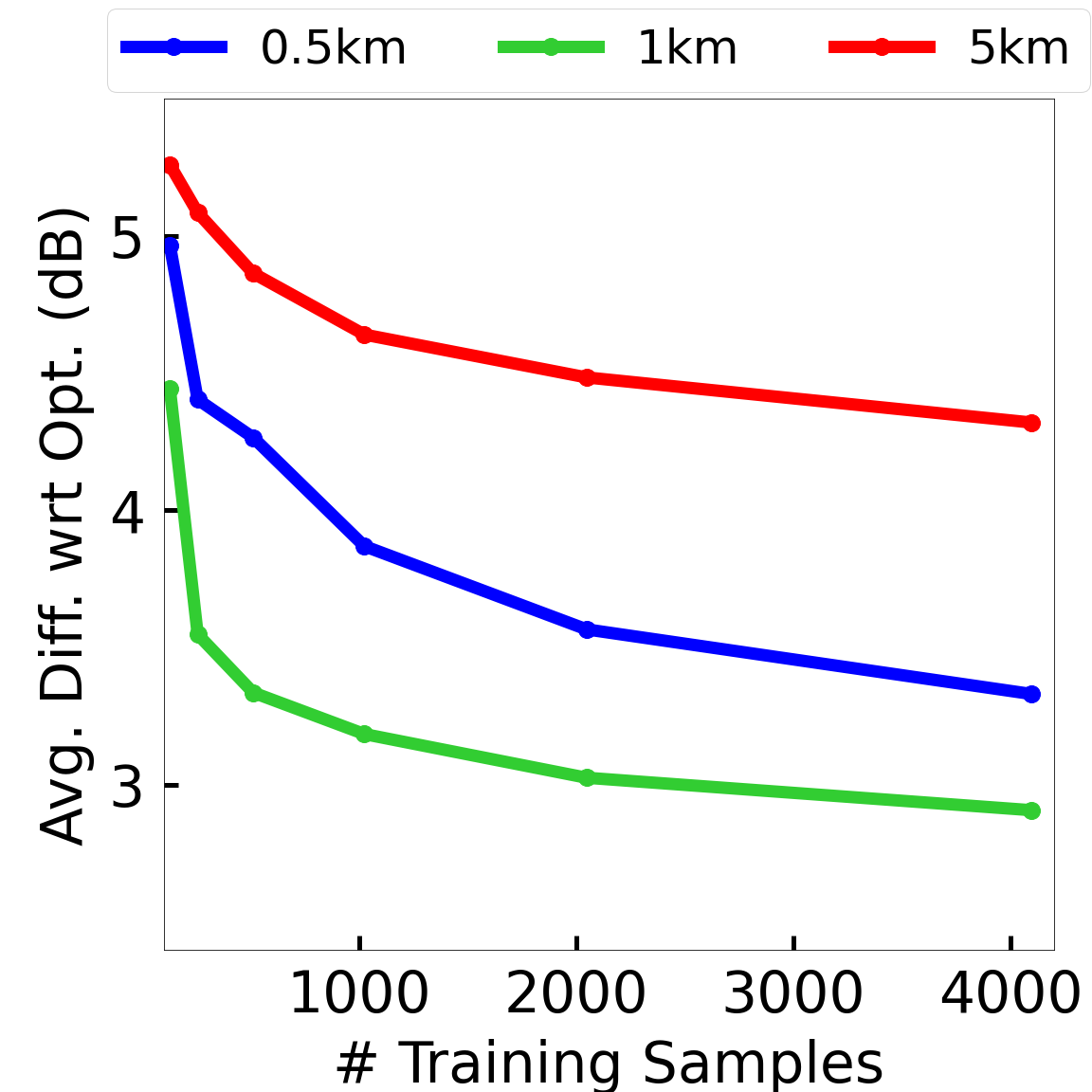
Multiple Regions. We also evaluated our DeepAlloc scheme over other regions with different sizes and terrain characteristics. See Fig. 10(a), which plots performance of DeepAlloc over three different regions—$500m\times 500m$ (our university campus), $1km\times 1km$ (airport landing area, the default region in all other plots), and $5km\times 5km$ (an urban area). We plot results for PU-Setting wherein the number of PUs is between 10 and 20. We see that DeepAlloc has an $\mathrm{\mathcal{A}_{err}}$ of 3-4.5 dB across all regions, and tt performs the best over the airport landing area likely due to lack of buildings and thus more uniform path-loss characteristics.

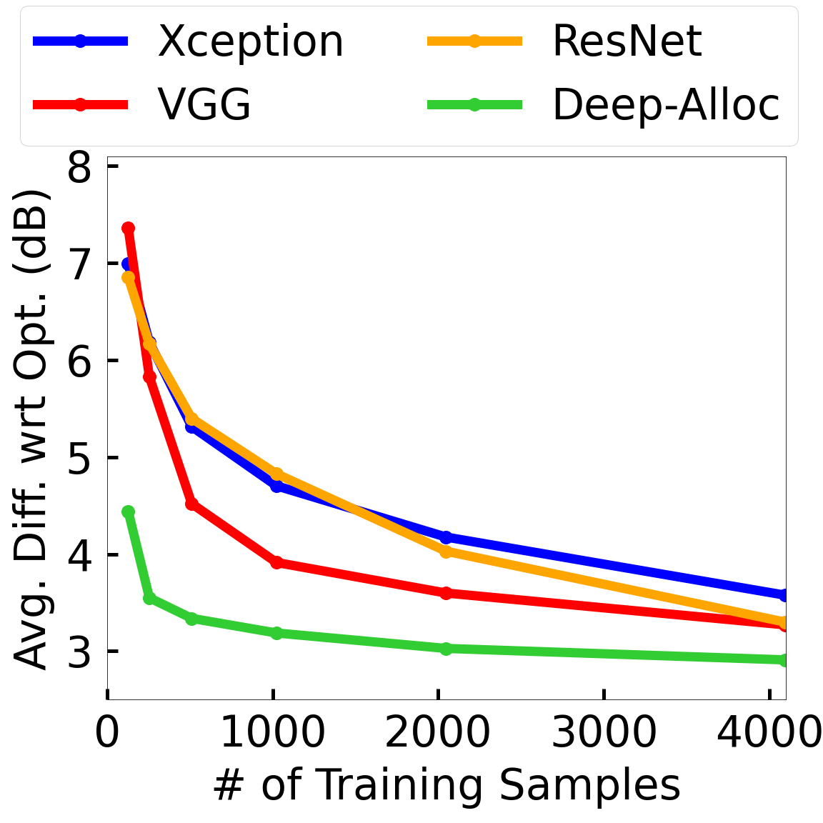
Various Pre-Trained Models. Finally, we present evaluation results for various pre-trained deep models. In particular, in addition to our DeepAlloc architecture, we also used some well-known Image Classification models such as VGG [40], ResNet [23], and Xception [15] which are all pre-trained with over 1 million images involving our daily-life objects; these pre-trained models were further trained with a varying number of (field-gathered) training samples. See Fig. 10(b), which plots the $\mathrm{\mathcal{A}_{err}}$ metric in PU-Setting for the above models compared with our DeepAlloc. We see that our approach of pre-training using log-normal model-based images in DeepAlloc yields a notable performance improvement; the performance gap is particularly significant for a lower number of training samples.

Computation Times and Complexity. The inference time complexity of all our ML approaches is linear in the size of the input, and thus, the inference time in practice is minimal (a fraction of a second). The training time complexity of most ML models depends on the training samples and the resulting convergence, and is thus, uncertain. The actual training times incurred from our set of training samples, on a 4GHz 8-core machine with a GeForce RTX 3080 GPU, were as follows: a few minutes for NN as well as SVR approaches, and a few hours for SH-Alloc. To train the DeepAlloc model, it took 5-7 days of computation time to pre-train the model using 1M images and a few hours to train/fine-tune the model after pre-training using SA training samples.

IV-B Multiple SUs/Channels

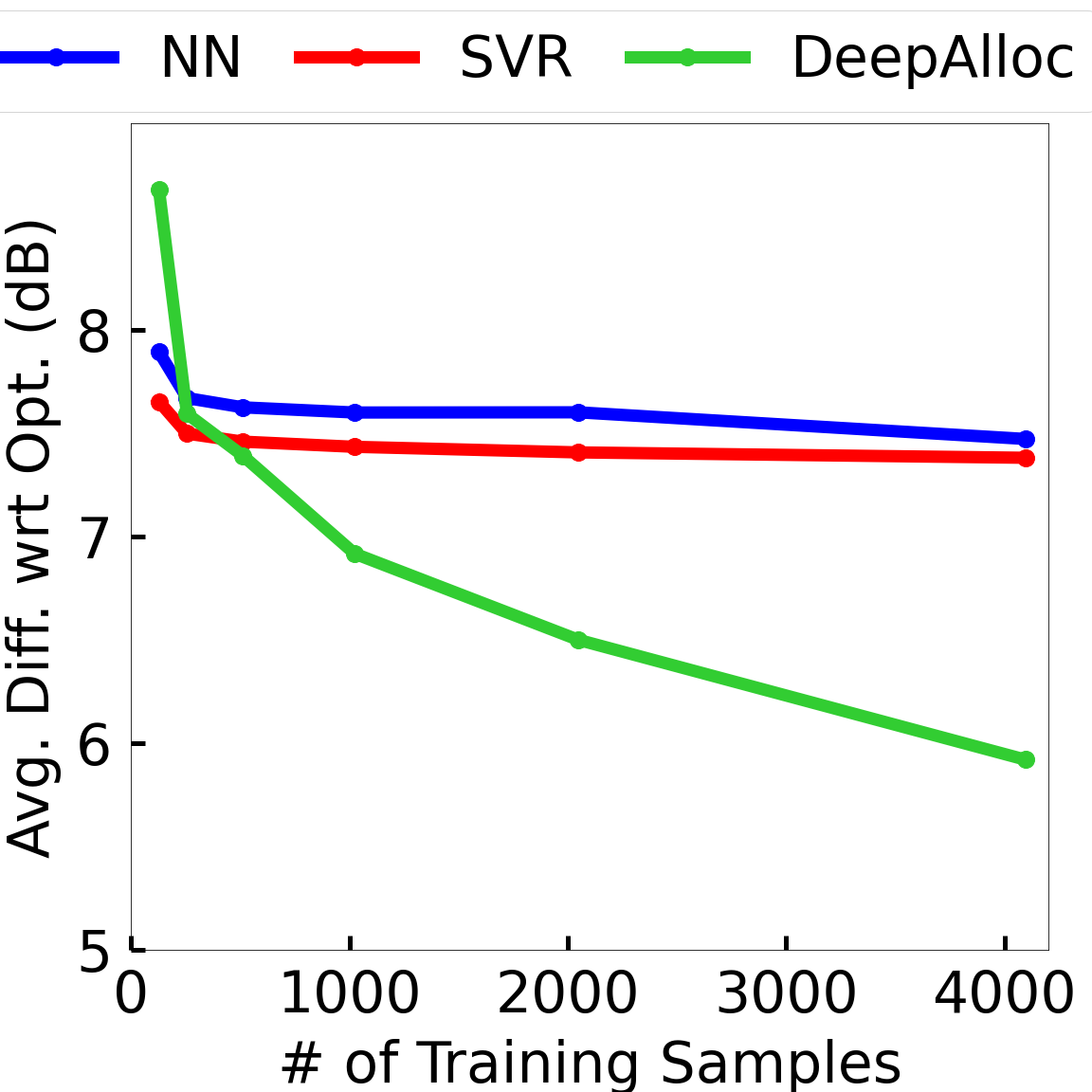
Subsequent SU. We start with comparing the spectrum power allocated to a single new SU with previous SUs being active. Each sample has a random number (between 1 and 10) of active SUs. For evaluation purposes, we assume that the active SUs are assigned the optimal power (as per Eqn. 1, with full knowledge of PU information and path-loss values) and they transmit using this optimal power. Then, the models predict the allocation power for the last requesting SU. See Fig. 11(a), which shows the performance of various ML algorithms in assigning the power to the last SU. We see that DeepAlloc easily outperforms the other ML approaches by a large margin. Also, not shown for clarity, but IP-Based had a poor $\mathrm{\mathcal{A}_{err}}$ of 21.6dB and SH-Alloc had a $\mathrm{\mathcal{A}_{err}}$’s of 7.5dB.

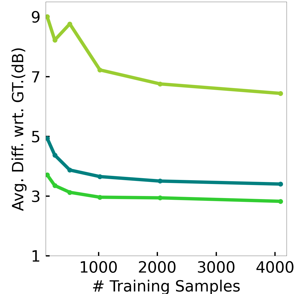
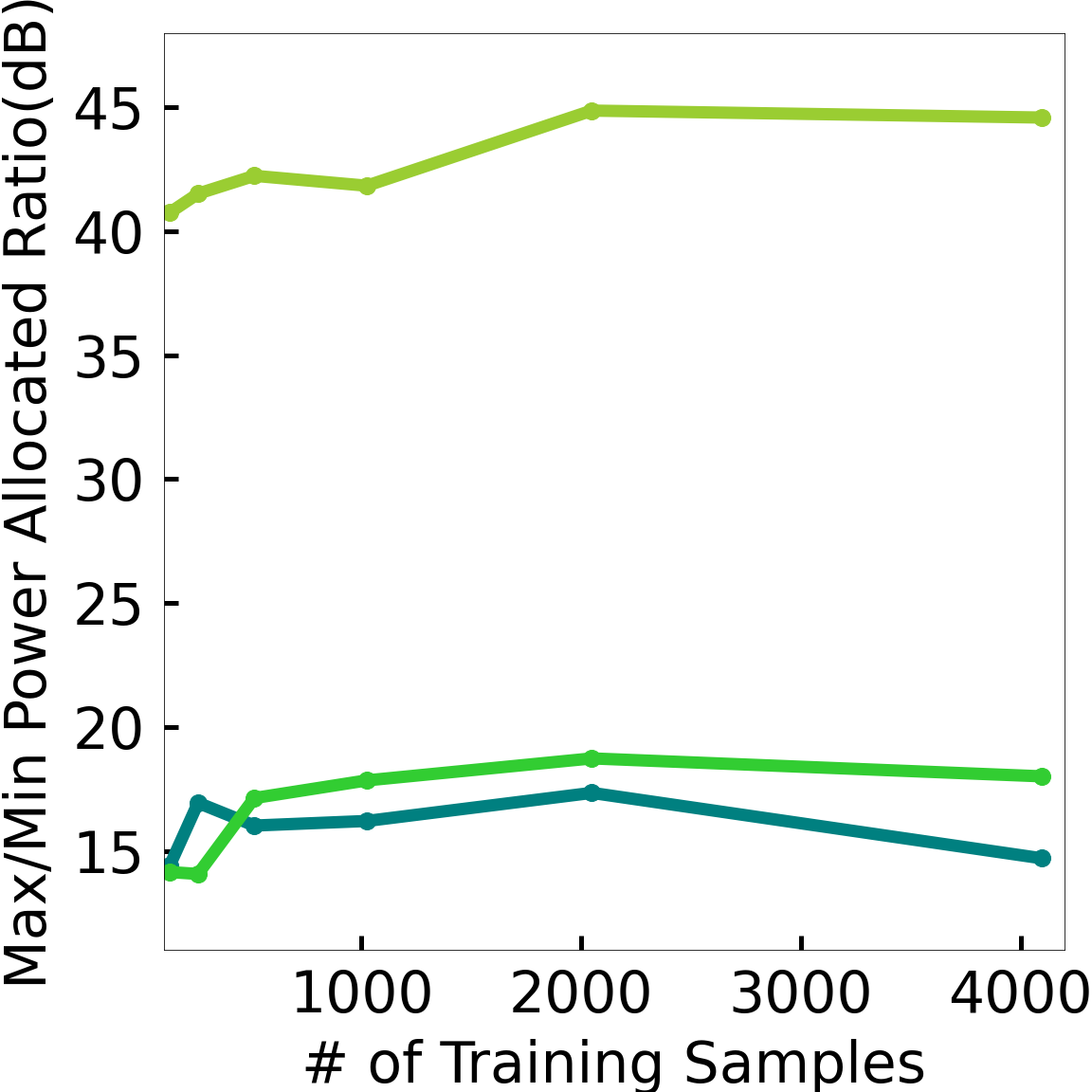
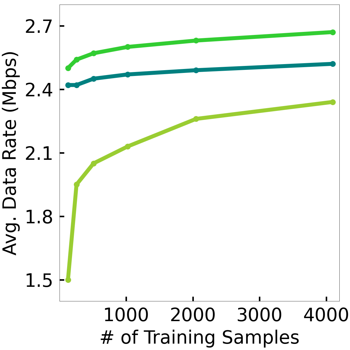
Concurrent SUs: Singular vs. Simultaneous Allocation. We now compare our approaches for handling concurrent SUs (§III-F), viz., DeepAlloc-Greedy, DeepAlloc-NN, and DeepAlloc-RNN; recall that the latter two approaches handle SUs simultaneously. We compare these algorithms in terms of (i) Average absolute-difference wrt to the ground truth (i.e., output of the Binary-Alloc heuristic); (ii) Fairness, in terms of the ratio of maximum to minimum power allocated to an SU; a lower value suggests a more fair allocation. (iii) Overall spectrum utilization, in terms of the total data rate achievable which is estimated as follows. For each SU, we assign a receiver in a random location around the SU (within 100m), calculate the total interference from PUs and other SUs at the receiver, and estimate the achievable data rate using Shannon’s capacity law. See Fig. 11(b)-(d). We observe that as expected the DeepAlloc-NN and DeepAlloc-RNN approaches that allocate powers simultaneously outperform DeepAlloc-Greedy significantly in all metrics, with DeepAlloc-RNN slightly outperforming the DeepAlloc-NN approach too (except in the fairness metric) which is not surprising as DeepAlloc-RNN has much more input information.

(a)

(a) Total allocated power.

(b) Fairness metric.

Figure 12: (a) Total allocated power, and (b) Fairness metric, in a four-channel setting with multiple SUs.

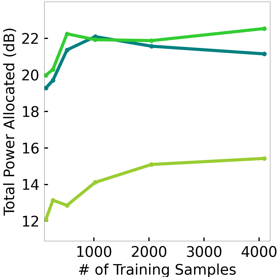
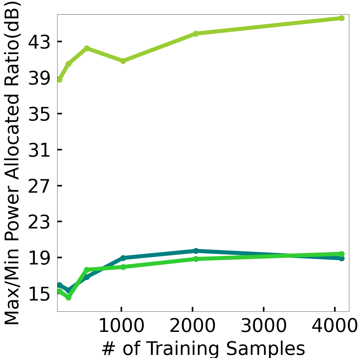
Multiple Channels. In Fig. 12, we compare our multi-SU approaches (tailored to multiple channels as described in §III-F) in the 4-channel PU-Setting with PUs transmitting over all the channels at all times. We allocate powers to 30 SUs. We observe that DeepAlloc-RNN still achieves the best performance in terms of total power allocation as well as fairness, with DeepAlloc-RNN performing closely. With respect to the single channel, the total power allocated is almost four times (in Watts).

(a) Devices

(b) Testbed Area

Figure 13: Outdoor testbed. (a) PU, PUR, SU, SS devices. (b) Testbed area (house backyard). Blue stars are the 17 sensors.

Figure 14: Testbed system overview, including the GNU-Radio based PU-to-PUR communication system .

(a)

(a) PU-Setting with 2-4 PUs.

(b) SS-Setting with 2-4 PUs, 17 SSs.

Figure 15: Testbed performance for increasing training set.

(a) Minimizing false positive error in PU-Setting.

(b) Handing multi-path effect in PU-Setting.

(c) Minimizing training cost via synthetic samples in PU-Setting.

(d) Minimizing training cost via synthetic samples in SS-Setting.

Figure 16: Evaluation of various aspects in the testbed.

V DeepAlloc TESTBED IMPLEMENTATION

In this section, we implement and evaluate a complete testbed system for our spectrum allocation system. We use the testbed to collect training samples, which are then used to train and evaluate the learned models. The testbed implementation demonstrates the effectiveness of our techniques in a realistic small-scale setting.

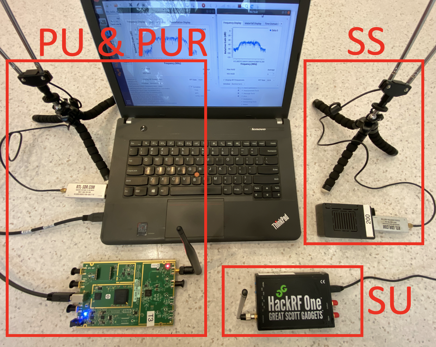
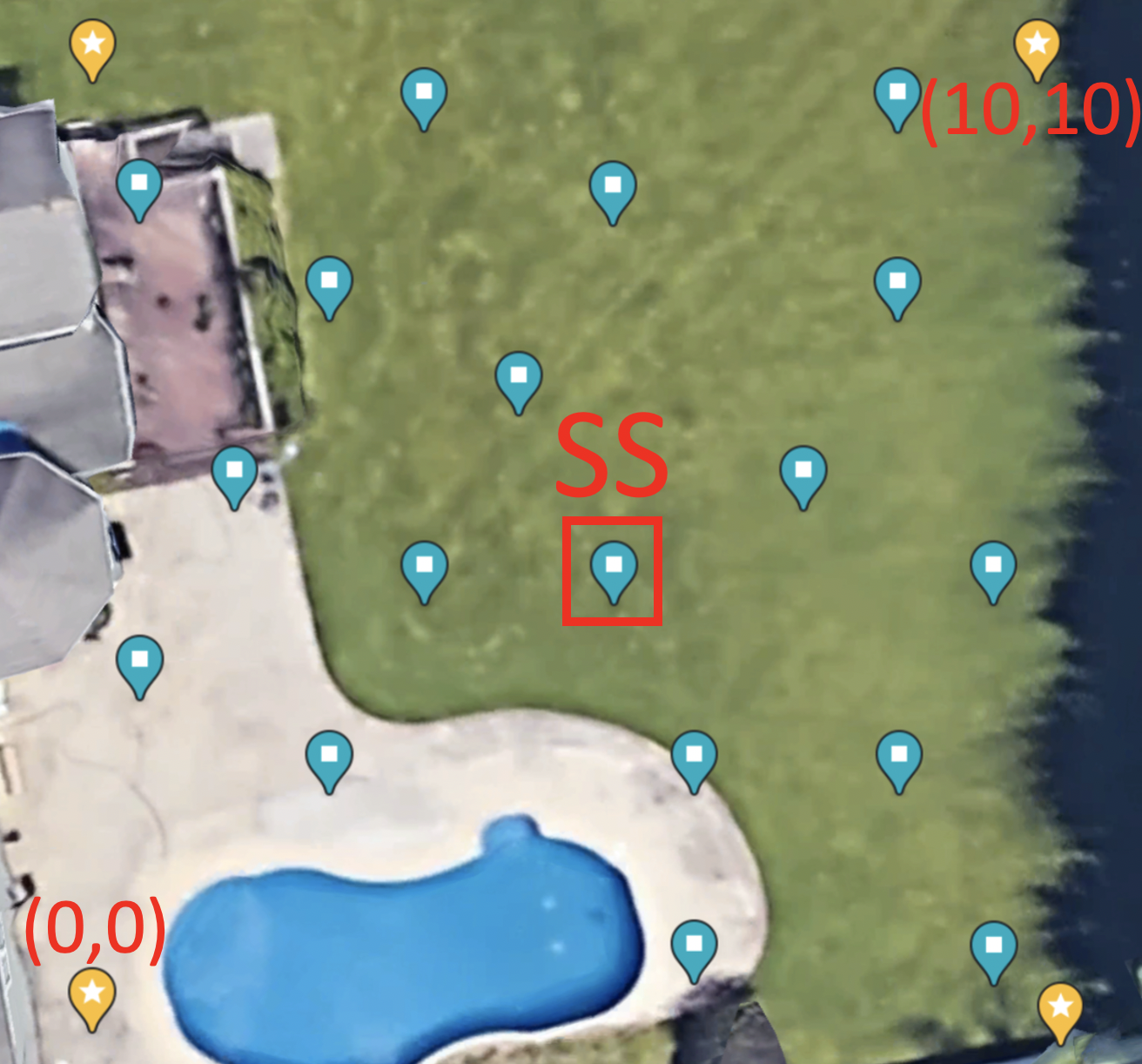
Transmitter and Receiver Devices Used. We use 4 USRP B200/B210 and 1 HackRF to play the role of the 4 PUs and 1 SU, respectively. A spectrum sensor (SS) is composed of an RTL-SDR dongle that connects to a dipole antenna and is powered by a single-board computer Odroid-C2. We deploy 17 of these spectrum sensors in the testbed. See Fig. 13(a). To simulate PU receivers (i.e., PURs), we use the same RTL-SDR dongle and antenna but power it by a laptop. Each PU is paired with one PUR, and they are both powered by a single laptop. Overall, we implemented a Python repository running on Linux that transmits and receives signals, and measures and collects relevant parameters in real time at 915 MHz ISM band at a sample rate of 1 MHz. We built our custom communication system based on GNU Radio for data communication between PU and PURs, used to determine labels (see below). See Fig. 14.

Collecting Training Samples. Recall that a sample in PU-Setting is comprised of a sample of PUs’ parameters (location and power) and the optimal power allocated to the SU. In SS-Setting, a training sample is comprised of spectrum sensors’ received power readings. The location of entities is available by using a GPS dongle connected to the laptops as described below, and the sensor’s received power is computed as follows. First, we compute an FFT on the I/Q samples collected within a time window to get a power spectral density (PSD) plot. Then, we compute the area under the PSD curve over the 1 MHz channel of interest (see below), and finally, convert the computed area to an appropriate unit.

Determining Labels (Optimal Power Allocated to SU). We essentially do a binary search to estimate the optimal power that can be allocated to SU. To determine whether PU to PUR transmission is incurring any harmful interference from SU, we have PU continuously streaming ASCII messages over the 1 MHz bandwidth channel centered at frequency 915.8 MHz, and check if the messages are successfully received at the PUR. This end-to-end communication system is implemented using GNU Radio.

Testbed Area and Setting. Due to the ongoing pandemic, the testbed was conducted in the backyard of a private house. The whole area is $24m\times 24m$ large. We divide the area into 100 grid cells where each represents $2.4m\times 2.4m$. See Figure 13(b). We use a GPS dongle that returns the location in (latitude, longitude) and the program converts it into coordinates. We determine the location of PU, SU, and the sensors with the help of GPS dongles and manual observation. All the Odroids and laptops are connected to an outdoor WiFi router and communicate through ssh protocol. For training and evaluation, the 17 sensing devices are placed on the ground and are uniformly spread out. PUs and SU are randomly placed in the area such that different regions of the backyard are ”covered”. PUs’ power is randomly assigned within a certain range.

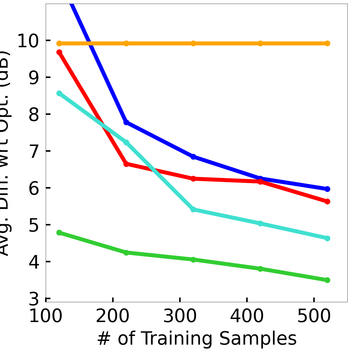
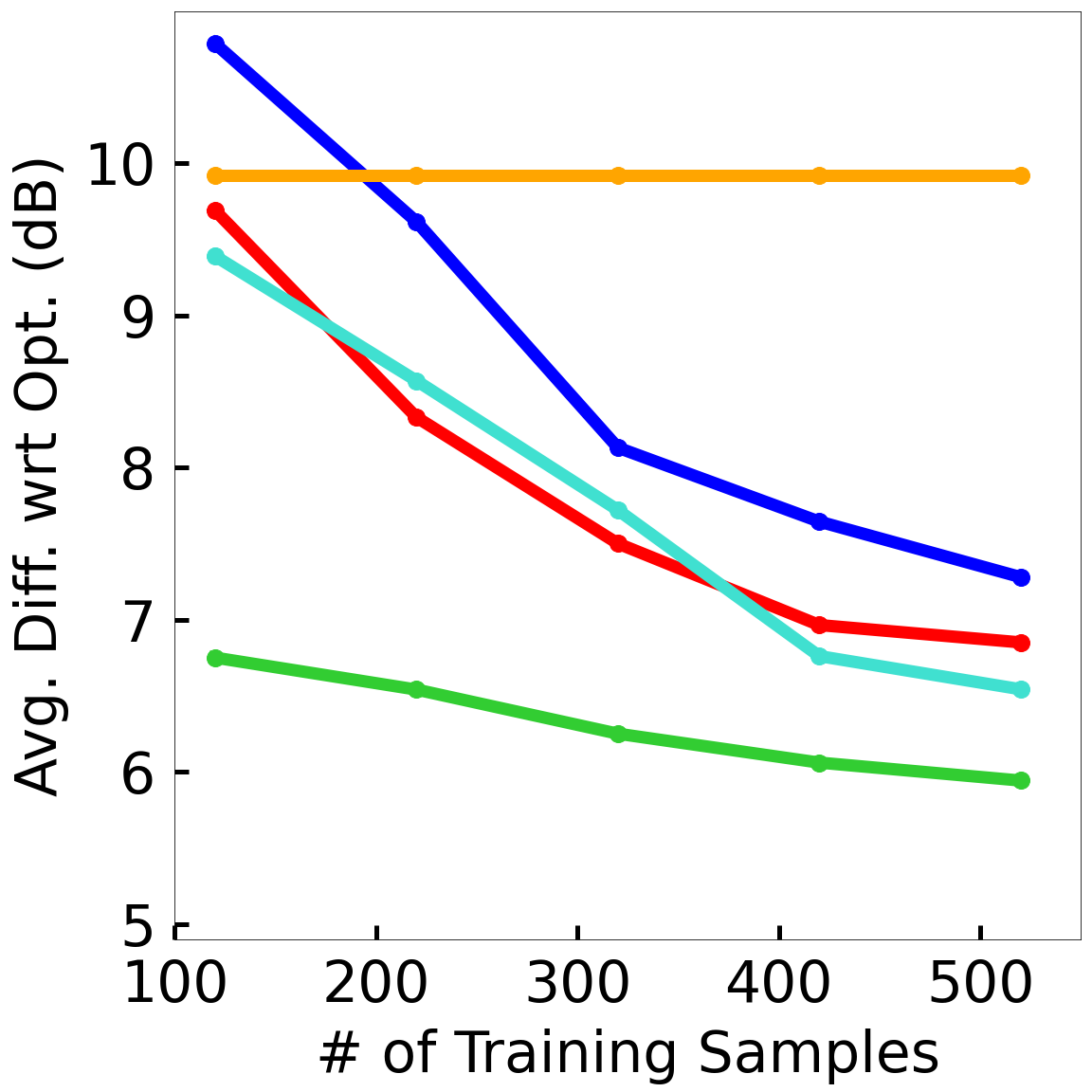
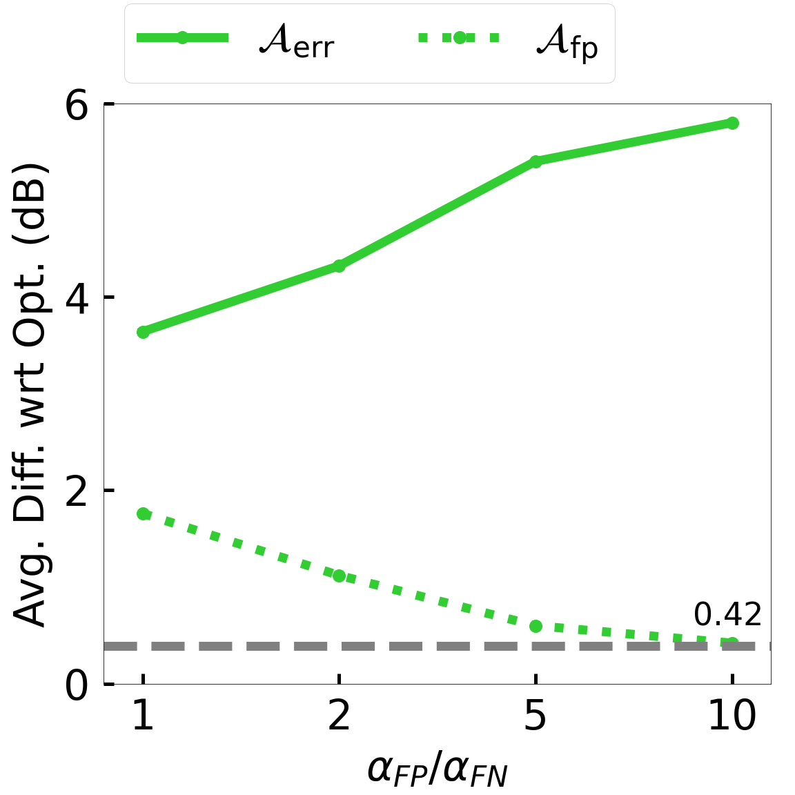
Results. First, we evaluate the performance of an increasing number of training samples. See Fig. 15. We observe a similar trend as in the previous section of large-scale simulation, with DeepAlloc outperforming other algorithms with a notable margin. In particular, the overall performance of DeepAlloc is good, with 4-5dB error using only 500 training samples. The performance of all algorithms is better in PU-Setting relative to the SS-Setting, as in §IV. Note that IP-Based performs quite poorly in this realistic setting, in spite of having knowledge of PU information as well as SS readings, as it assumes an imprecise propagation model. Finally, we evaluate our techniques to handle various aspects, viz., false positive error, multi-path effect, and synthetic samples in Fig. 16. Overall, we observe a similar trend as in the large-scale simulations.

VI Conclusions

We have developed an effective deep-learning technique based on CNNs to learn the spectrum allocation function, and have demonstrated its effectiveness via extensive large-scale simulations as well as a small outdoor testbed. There are many avenues for further improvement of our techniques. First, one could easily pre-train the DeepAlloc model with a much larger number of pre-training samples; as our pre-training samples can be automatically generated, this only incurs additional computational cost but no additional field training/deployment cost. Second, we could also use a more sophisticated models to generate high-fidelity pre-training samples. Lastly, we could incorporate terrain information in the image sheets to aid the learning process. These directions form the focus of our future work.

Mohammad Ghaderibaneh received the B.S. degree in electrical engineering from Azad University, Urmia, Iran in 2008 and the M.S. degree in telecommunication engineering from Shahid Beheshti University, Tehran, Iran in 2011. He received his Ph.D. degree in computer science at Stony Brook University, NY, USA in 2023. From 2012 to 2018, he worked in the industry as a Software and Telecommunication Engineer developing wireless communication networks like TETRA. He now works at Google YouTube. His research interests include quantum networks and machine learning application in wireless networks.

Caitao Zhan received his B.S. degree in computer science and technology from China University of Geosciences in Wuhan, China in 2017. He then joined the PhD program at Stony Brook University at the Department of Computer Science and is now a PhD candidate. He does research in the broad area of computer networks and his interest lies at the intersection of wireless networks and machine learning. He is also interested in quantum communication and quantum sensing.

Himanshu Gupta is a professor of computer science at Stony Brook University, where he has been a faculty since 2002. His area of research has been in wireless networks, with recent focus on free-space optical communication networks and spectrum management. His current research focuses on quantum networks and communication, and distributed quantum algorithms. He graduated with an M.S. and Ph.D. in Computer Science from Stanford University in 1999, and a B.Tech. in Computer Science and Engineering from IIT Bombay in 1992.

References

- [1] FCC 3.5GHz Band. "https://www.fcc.gov/wireless/bureau-divisions/mobility-division/35-ghz-band/35-ghz-band-overview.
- [2] FCC White Space. https://www.fcc.gov/general/white-space.
- [3] DeepAlloc’s source code repository, 2023. https://github.com/Wings-Lab/SpectrumAllocationDL.
- [4] Jeffrey G. Andrews, Stefano Buzzi, et al. What will 5g be? IEEE Journal on Selected Areas in Communications, 2014.
- [5] F. Azmat, Y. Chen, and N. Stocks. Analysis of spectrum occupancy using machine learning algorithms. IEEE Transactions on Vehicular Technology, Sep. 2016.
- [6] Yoshua Bengio, Ian Goodfellow, and Aaron Courville. Deep learning, volume 1. MIT press Massachusetts, USA:, 2017.
- [7] Sudeep Bhattarai et al. An overview of dynamic spectrum sharing: Ongoing initiatives, challenges, and a roadmap for future research. IEEE TCCN, 2016.
- [8] Milind M. Buddhikot et al. Dimsumnet: new directions in wireless networking using coordinated dynamic spectrum. In IEEE WOWMOM, June 2005.
- [9] S. Byun et al. Dynamic spectrum allocation in wireless cognitive sensor networks: Improving fairness and energy efficiency. In IEEE VTC, 2008.
- [10] Roberto Calvo-Palomino, Domenico Giustiniano, Vincent Lenders, and Aymen Fakhreddine. Crowdsourcing spectrum data decoding. In IEEE INFOCOM, 2017.
- [11] Ayon Chakraborty and Samir R. Das. Measurement-augmented spectrum databases for white space spectrum. In CoNEXT, 2014.
- [12] Ayon Chakraborty, M. S. Rahman, H. Gupta, and S. Das. Specsense: Crowdsensing for efficient querying of spectrum occupancy. In IEEE INFOCOM, 2017.
- [13] K. Chamberlin and R. Luebbers. An evaluation of longley-rice and gtd propagation models. IEEE Transactions on Antennas and Propagation, November 1982.
- [14] Wentai Chen et al. A reinforcement learning based joint spectrum allocation and power control algorithm for D2D communication underlaying cellular networks. In AICON, 2019.
- [15] F. Chollet. Xception: Deep learning with depthwise separable convolutions, 2017.
- [16] Max Curran, Xiao Liang, Himanshu Gupta, Omkant Pandey, and S. Das. Procsa: Protecting privacy in crowdsourced spectrum allocation. In ESORICS, 2019.
- [17] Y. Dou, K. Zeng, et al. -SAS: Privacy-preserving centralized dynamic spectrum access system. IEEE Journal on Selected Areas in Communications, Jan 2017.
- [18] Harris Drucker, Christopher JC Burges, Linda Kaufman, Alex J Smola, and Vladimir Vapnik. Support vector regression machines. In NeurIPS, 1997.
- [19] M. El Tanab and W. Hamouda. Resource allocation for underlay cognitive radio networks: A survey. IEEE Communications Surveys Tutorials, 2017.
- [20] S. Gao, L. Qian, and D. R. Vaman. Distributed energy efficient spectrum access in wireless cognitive radio sensor networks. In WCNC, 2008.
- [21] Euhanna Ghadimi, Francesco Davide Calabrese, Gunnar Peters, and Pablo Soldati. A reinforcement learning approach to power control and rate adaptation in cellular networks. In 2017 IEEE International Conference on Communications (ICC), pages 1–7, 2017.
- [22] H. Gupta, M. Rahman, and M. Curran. Shared spectrum allocation via pathloss estimation in crowdsensed shared spectrum systems. In DySPAN, Nov 2019.
- [23] Kaiming He, Xiangyu Zhang, Shaoqing Ren, and Jian Sun. Deep residual learning for image recognition. In IEEE CVPR, 2016.
- [24] S. He, D. Shin, J. Zhang, and J. Chen. Toward optimal allocation of location dependent tasks in crowdsensing. In IEEE INFOCOM, 2014.
- [25] A. T. Hoang et al. Power control and channel allocation in cognitive radio networks with primary users’ cooperation. IEEE TMC, March 2010.
- [26] P. Karimi, W. Lehr, I. Seskar, and D. Raychaudhuri. Smap: A scalable and distributed architecture for dynamic spectrum management. In DySPAN, Oct 2018.
- [27] Diederik P Kingma and Jimmy Ba. Adam: A method for stochastic optimization. arXiv preprint arXiv:1412.6980, 2014.
- [28] W. Lee and I. F. Akyldiz. A spectrum decision framework for cognitive radio networks. IEEE Transactions on Mobile Computing, 2011.
- [29] Alexe E Leu et al. Modeling and analysis of interference in listen-before-talk spectrum access schemes. International Journal of Network Management, 2006.
- [30] Xiukui Li and Seyed A. (Reza) Zekavat. Distributed channel assignment in cognitive radio networks. In IWCMC, 2009.
- [31] J. A. Magliacane. Splat! a terrestrial rf path analysis application for linux/unix. Downloaded from https://www.qsl.net/kd2bd/splat.html, 2008.
- [32] A. Medeisis and A. Kajackas. On the use of the universal okumura-hata propagation prediction model in rural areas. In IEEE VTC, May 2000.
- [33] Fan Meng, Peng Chen, Lenan Wu, and Julian Cheng. Power allocation in multi-user cellular networks: Deep reinforcement learning approaches. IEEE Transactions on Wireless Communications, 19(10):6255–6267, 2020.
- [34] Nils Morozs. Accelerating Reinforcement Learning for Dynamic Spectrum Access in Cognitive Wireless Networks. PhD thesis, University of York, 2015.
- [35] Vinod Nair and Geoffrey E Hinton. Rectified linear units improve restricted boltzmann machines. In ICML, 2010.
- [36] Yasar Sinan Nasir and Dongning Guo. Deep reinforcement learning for joint spectrum and power allocation in cellular networks. In 2021 IEEE Globecom Workshops (GC Wkshps), pages 1–6, 2021.
- [37] H. Salameh. Throughput-oriented channel assignment for opportunistic spectrum access networks. Mathematical and Computer Modelling, 2011.
- [38] P Mohana Shankar. Fading and shadowing in wireless systems. Springer, 2017.
- [39] J. Shi, Z. Guan, C. Qiao, T. Melodia, G. Challen, et al. Crowdsourcing access network spectrum allocation using smartphones. In HotNets, 2014.
- [40] Karen Simonyan and Andrew Zisserman. Very deep convolutional networks for large-scale image recognition. In ICLR, 2015.
- [41] Y. Song, K. W. Sung, and Y. Han. Coexistence of wi-fi and cellular with listen-before-talk in unlicensed spectrum. IEEE Communications Letters, 2016.
- [42] E. Z. Tragos et al. Spectrum assignment in cognitive radio networks: A comprehensive survey. IEEE Communications Surveys Tutorials, 2013.
- [43] M. Uccellari, F. Facchini, et al. On the application of support vector machines to the prediction of propagation losses at 169mhz for smart metering applications. IET Microwaves, Antennas Propagation, 2018.
- [44] H. Wang, J. Ren, and T. Li. Resource allocation with load balancing for cognitive radio networks. In GlobCom, 2010.
- [45] W. Wang, K. G. Shin, and W. Wang. Joint spectrum allocation and power control for multihop cognitive radio networks. IEEE TMC, 2011.
- [46] Yonghua Wang et al. A survey of dynamic spectrum allocation based on reinforcement learning algorithms in cognitive radio networks. AIR, 2019.
- [47] L. Yu, C. Liu, and W. Hu. Spectrum allocation algorithm in cognitive ad-hoc networks with high energy efficiency. In ICGCS, 2010.
- [48] H. Zhang, N. Yang, W. Huangfu, K. Long, and V. C. M. Leung. Power control based on deep reinforcement learning for spectrum sharing. IEEE TWC, 2020.
- [49] Yong Zhang, Canping Kang, Tengteng Ma, Yinglei Teng, and Da Guo. Power allocation in multi-cell networks using deep reinforcement learning. In 2018 IEEE 88th Vehicular Technology Conference (VTC-Fall), pages 1–6, 2018.
- [50] Q. Zhao and B. M. Sadler. A survey of dynamic spectrum access. IEEE Signal Processing Magazine, 2007.
![[Uncaptioned image]](/html/2201.07762/assets/figures/people/mg.jpg) |