Wannier Functions Dually Localized in Space and Energy

Abstract

Wannier functions are real-space representations of Bloch orbitals that provide a useful picture for chemical bonding and offer a localized description of single-particle wave functions. There is a unitary freedom in the construction of Wannier functions from Bloch orbitals, which can be chosen to produce Wannier functions that have advantageous properties. A popular choice for this freedom is the minimization of spatial variance, which leads to maximally localized Wannier functions. We minimize a weighted sum of the spatial and energy variances, yielding what we call dually localized Wannier functions. Localization in energy results in Wannier functions that are associated with a particular energy and allows for dually localized Wannier functions to be comprised of occupied and unoccupied spaces simulatneously. This can lead to Wannier functions that are fractionally occupied, which is a key feature that is used in correcting the delocalization error in density functional approximations. We show how this type of localization results in bonding (antibonding) functions for the occupied (unoccupied) spaces around the frontier energy of silicon in the diamond lattice and of molecular ethylene. Dually localized Wannier functions therefore offer a relevant description for chemical bonding and are well suited to orbital-dependent methods that associate Wannier functions with specific energy ranges without the need to consider the occupied and unoccupied spaces separately.

I Introduction

In the single-particle picture of electronic structure theory, the eigenfunctions of the Hamiltonian may be delocalized in space. This is especially true when the Hamiltonian is periodic and the solutions are Bloch functions $\psi_{n}^{\mathbf{k}}(\mathbf{r})=e^{i\mathbf{k}\cdot\mathbf{r}}u_{n}^{\mathbf{k}}(\mathbf{r})$, where $u_{n}^{\mathbf{k}}(\mathbf{r})$ shares the periodicity of the Hamiltonian. Bloch functions are indexed by $\mathbf{k}$, a point in reciprocal space, and a band index corresponding to the $n^{\text{th}}$ eigenvalue for that $\mathbf{k}$-point, i.e., $H\psi_{n}^{\mathbf{k}}=\epsilon_{n}^{\mathbf{k}}\psi_{n}^{\mathbf{k}}$. As can be seen from the plane wave $e^{i\mathbf{k}\cdot\mathbf{r}}$ in their definition, the Bloch orbitals are delocalized in space while being perfectly localized in energy, limiting their utility in describing spatially local properties such as chemical bonds. Dual to the Bloch orbitals are the Wannier functions, which are the Fourier transform of the Bloch orbitals over the Brillouin zone [1]. They are localized in real space, making them useful for evaluating position-dependent quantities such as the dipole moment [2, 3], as a basis set for large-scale simulations [4, 5, 6, 7], interpolating band structures [8], as a picture of chemical bonding [9, 10], and as localized orbitals in orbital-dependent methods [11, 12, 13, 14].

If a finite number $N_{k}$ of $\mathbf{k}$-points in the first Brillouin zone are sampled, Wannier functions take the form

$$\lvert w_{n}^{\mathbf{R}}\rangle=\frac{1}{N_{k}}\sum_{\mathbf{k}}e^{-i\mathbf{k}\cdot\mathbf{R}}\lvert\psi_{n}^{\mathbf{k}}\rangle,$$ (1)

where $\mathbf{R}$ indexes unit cells in the unfolded supercell on which the Wannier functions are periodic. Equal weighting of all $\mathbf{k}$-points is equivalent to sampling on a Monkhorst-Pack mesh [15], which we assume throughout the text. This $\mathbf{k}$-sampling procedure also yields Wannier functions that are periodic on an unfolded supercell obeying Born–von Karman boundary conditions, with the number of primitive unit cells in each real-space lattice direction equal to the number of $\mathbf{k}$-points sampled in the corresponding reciprocal lattice direction [16]. The Fourier transform normalization convention in Eq. (1) also implies a Bloch orbital normalization $\langle\psi_{n}^{\mathbf{k}}|\psi_{m}^{\mathbf{q}}\rangle=N_{k}\delta_{nm}\delta_{\mathbf{k}\mathbf{q}}$. The inverse transform from Bloch orbital to Wannier function is then

$$\lvert\psi_{n}^{\mathbf{k}}\rangle=\sum_{\mathbf{R}}e^{i\mathbf{k}\cdot\mathbf{R}}\lvert w_{n}^{\mathbf{R}}\rangle.$$ (2)

Since the Bloch orbitals are eigenfunctions, they have a phase freedom in their formulation. This leads to a gauge freedom in the construction of the Wannier functions:

$$\begin{split}\lvert w_{n}^{\mathbf{R}}\rangle&=\frac{1}{N_{k}}\sum_{\mathbf{k}}e^{-i\mathbf{k}\cdot\mathbf{R}}e^{i\theta_{n}(\mathbf{k})}\lvert\psi_{n}^{\mathbf{k}}\rangle.\end{split}$$ (3)

For obtaining localized Wannier functions, a natural choice for this gauge freedom is to choose the phase factors $\theta_{n}(\mathbf{k})$ such that $\lvert\psi_{n}^{\mathbf{k}}\rangle$ is as smooth as possible in its dependence on $\mathbf{k}$. If it is analytic, the resulting Wannier function is exponentially localized [17]. However, multiple bands may cross one another in the Brillouin zone, yielding $\mathbf{k}$-points with a set of degenerate Bloch functions. Any unitary combination $U^{\mathbf{k}}$ of the degenerate bands remains a set of eigenfunctions of the Hamiltonian. These freedoms lead to generalized Wannier functions, which allows the bands to mix at a fixed $\mathbf{k}$-point by an arbitrary unitary operator $U^{\mathbf{k}}$ [18],

$$\begin{split}\lvert w_{n}^{\mathbf{R}}\rangle&=\frac{1}{N_{k}}\sum_{\mathbf{k}}e^{-i\mathbf{k}\cdot\mathbf{R}}\sum_{m}U_{mn}^{\mathbf{k}}\lvert\psi_{m}^{\mathbf{k}}\rangle\\ &=\frac{1}{N_{k}}\sum_{\mathbf{k}}e^{-i\mathbf{k}\cdot\mathbf{R}}\lvert\phi_{n}^{\mathbf{k}}\rangle.\end{split}$$ (4)

We call the set $\{\lvert\phi_{n}^{\mathbf{k}}\rangle\}$ the transformed Bloch orbitals. Thus, a generalized Wannier function can be comprised of a combination of bands, and the combination may vary across the Brillouin zone.

I.1 Cost functions

The unitary freedom in the construction of the Wannier functions can be chosen to satisfy a desired criterion. In the case of the maximally localized Wannier functions (MLWFs) proposed by Marzari and Vanderbilt [9], the $U^{\mathbf{k}}$ minimize the spatial variance

$$\begin{split}\Omega&=\sum_{n}\langle w_{n}|\Delta r^{2}|w_{n}\rangle,\\ \end{split}$$ (5)

where $\langle f|x|g\rangle=\int_{\mathcal{D}}d\mathbf{r}\,f^{*}(\mathbf{r})x(\mathbf{r})g(\mathbf{r})$ for any operator $x$ and functions $f,g$. The domain of integration $\mathcal{D}$ depends on the periodicity of $f$ and $g$. In the case of the Wannier functions, $\mathcal{D}$ is the Born–von Karman unit cell [16]. We write $\langle\Delta x^{2}\rangle=\langle x^{2}\rangle-\lvert\langle{x}\rangle\rvert^{2}$ for the variance of $x$. Note that the MLWF localization cost function of Eq. (5) is the bulk-system extension of the Foster-Boys localization for finite systems [19]. The Wannier functions are translationally symmetric on the primitive unit cell, so without loss of generality we only include the Wannier functions indexed by the home unit cell, $\mathbf{R}=\mathbf{0}$. Summing over all unit cells $\mathbf{R}$ in the Born–von Karman unit cell would only change the cost function by a multiplicative constant. The MLWF formulation was originally applied to a composite set of energy bands, which is a set of Bloch orbitals separated by an energy gap from all other states at every point in the Brillouin zone. The gradient of $\Omega$ was shown analytically for a composite set by Marzari and Vanderbilt [9], and descent methods are applied to obtain the $U^{\mathbf{k}}$ which minimize $\Omega$. Applied to the occupied orbitals of gapped systems with vanishing Chern numbers, MLWFs have been proven to be real and exponentially localized in three and fewer dimensions [20, 17, 21, 22].

We now introduce the dual localization criteria, adding an energy variance term to the MLWF cost function:

$$\begin{split}F&=(1-\gamma)\sum_{n}\langle w_{n}|\Delta r^{2}|w_{n}\rangle+\gamma\sum_{n}\langle w_{n}|\Delta h^{2}|w_{n}\rangle\\ &=(1-\gamma)\Omega+\gamma\Xi,\end{split}$$ (6)

where $h$ is the single-particle Hamiltonian, $\Omega$ denotes the spatial spread, and $\Xi$ denotes the energy spread. The mixing term $\gamma$ can be tuned to prioritize spatial or energy localization (see Sec. II.4). This cost function was used in the localized orbital scaling correction (LOSC) [23], which aims to systemically eliminate delocalization error using localized orbitals [24]. In the case of finite systems, the localized orbitals based on the optimization of the cost function, Eq. (6) are called orbitalets to highlight its space and energy localization [24, 23]. The form of $F$ was first suggested by Gygi et al. in [25]; however, the algorithm there proposed is only applicable to $\Gamma$-sampled systems, where the Brillouin zone is sampled only at the origin. In that case, the transformed Bloch orbitals are equivalent to the Wannier functions, and varying the mixing term $\gamma$ progresses between MLWFs and Bloch orbitals. Additionally, the $\Gamma$-only algorithm does not offer guidance on how to treat both occupied and unoccupied spaces together. We show how using the cost function in Eq. (6) can produce physically meaningful localizations when any number of virtual orbitals are included in its domain. The resulting Wannier functions are localized in both space and energy; we therefore refer to them as dually localized Wannier functions (DLWFs).

I.2 Occupied and unoccupied spaces

The inclusion of energy localization allows occupied and unoccupied Bloch orbitals to be considered together for Wannier function construction. When using a cost function that solely minimizes spatial variance, only a set of Bloch bands that are close together in energy are typically used to construct MLWFs. This is because the basis of Hamiltonian eigenstates is complete and the MLWF cost function allows Bloch bands to mix freely regardless of their relative energy. Adding more bands to the construction of MLWFs will therefore yield states arbitrarily localized in space, while losing virtually all information about the energy content carried by the Bloch bands from which they were constructed. On the other hand, if energy variance is included in addition to spatial variance, then the mixing of Bloch orbitals that are far apart in energy is suppressed. This means that a set of Bloch orbitals spanning a large energy range can be considered and results in Wannier functions that are localized in space as well as associated with a particular energy.

When there is an energy gap between the occupied and unoccupied Bloch orbitals, a set of Wannier functions can be comprised of the occupied Bloch orbitals, and the projector onto the occupied space may be written in the Bloch orbital or Wannier function basis as

$$\begin{split}P_{\text{occ}}&=\frac{1}{N_{k}}\sum_{n\mathbf{k}}f_{n}^{\mathbf{k}}\lvert\psi_{n}^{\mathbf{k}}\rangle\!\langle\psi_{n}^{\mathbf{k}}\rvert\\ &=\sum_{n\mathbf{R}}f_{n}^{\mathbf{R}}\lvert w_{n}^{\mathbf{R}}\rangle\!\langle w_{n}^{\mathbf{R}}\rvert,\end{split}$$ (7)

where $f_{n}^{\mathbf{k}},f_{n}^{\mathbf{R}}\in\{0,1\}$ are the occupations of the Bloch orbitals and Wannier functions respectively. When the set of Wannier functions includes both occupied and unoccupied bands, the Wannier functions may not have integer occupancy: that is, $\langle w_{n}^{\mathbf{R}}|P_{\text{occ}}|w_{n}^{\mathbf{R}}\rangle\not\in\{0,1\}$. The fractional occupiations were used in the LOSC approach to correct the major underestimation of the total energy in molecular ions at large bond length, which is caused by the delocalization error in the functional approximation. Fractional occupation also means the occupied projector $P_{\text{occ}}$ is no longer diagonal in the transformed band index $n$. If the transformed bands include all of the occupied Bloch orbitals, the occupied projector can be written using the transformed Bloch orbitals as

$$\begin{split}P_{\text{occ}}&=\frac{1}{N_{k}^{2}}\sum_{m\mathbf{q}}\sum_{n\mathbf{k}}\left(\langle\phi_{m}^{\mathbf{q}}|P_{\text{occ}}|\phi_{n}^{\mathbf{k}}\rangle\right)\lvert\phi_{m}^{\mathbf{q}}\rangle\!\langle\phi_{n}^{\mathbf{k}}\rvert\\ &=\frac{1}{N_{k}}\sum_{mn\mathbf{k}}\lambda_{mn}^{\mathbf{k}}\,\lvert\phi_{m}^{\mathbf{k}}\rangle\!\langle\phi_{n}^{\mathbf{k}}\rvert,\end{split}$$ (8)

where $\lvert\phi_{n}^{\mathbf{k}}\rangle=\sum_{m}U_{mn}^{\mathbf{k}}\lvert\psi_{m}^{\mathbf{k}}\rangle$ is a transformed Bloch orbital. The $\lambda_{mn}^{\mathbf{k}}$ can be viewed as local occupations of the transformed Bloch functions; observe that the matrix $[\Lambda^{\mathbf{k}}]_{mn}=\lambda_{mn}^{\mathbf{k}}$ is not necessarily diagonal in $n$ as it is when the Wannier functions are constructed only from occupied Bloch bands. The trace of $\Lambda^{\mathbf{k}}$ is $N_{f}^{\mathbf{k}}$, the number of Bloch states below the Fermi energy at $\mathbf{k}$. For simplicity, we have omitted the spin index, but these arguments also apply to open-shell systems, albeit for each spin channel independently. As the unitary transform of a diagonal projector, $\Lambda^{\mathbf{k}}$ is a Hermitian matrix with $0\leq\lambda_{ii}^{\mathbf{k}}\leq 1$.

We can also write the occupied projector in terms of the Wannier functions as

$$\begin{split}P_{\text{occ}}&=\sum_{m\mathbf{R}}\sum_{n\mathbf{T}}\left(\langle w_{m}^{\mathbf{R}}|P_{\text{occ}}|w_{n}^{\mathbf{T}}\rangle\right)\lvert w_{m}^{\mathbf{R}}\rangle\!\langle w_{n}^{\mathbf{T}}\rvert\\ &=\sum_{\mathbf{R}\mathbf{T}}\sum_{mn}\lambda_{mn}^{\mathbf{R}\mathbf{T}}\,\lvert w_{m}^{\mathbf{R}}\rangle\!\langle w_{n}^{\mathbf{T}}\rvert.\end{split}$$ (9)

The matrix $[\Lambda^{\mathbf{R}\mathbf{T}}]_{mn}=\lambda_{mn}^{\mathbf{R}\mathbf{T}}$ is the element-wise discrete Fourier transform of the occupation matrix $\Lambda^{\mathbf{k}}$ of transformed Bloch orbitals. $\Lambda^{\mathbf{R}\mathbf{T}}$ can be viewed as the occupation matrix of the Wannier functions; restricted to the home cell, it has unit cell trace $\operatorname{Tr}_{c}[\Lambda^{(\mathbf{0}\mathbf{0})}]=\sum_{n}\Lambda^{(\mathbf{0}\mathbf{0})}_{nn}=N_{k}^{\text{-}1}\sum_{k}N_{f}^{\mathbf{k}}$.

II Methods

The procedure outlined by Marzari and Vanderbilt in [9] detailed how to find the analytic gradient for minimizing $\Omega$ for a composite set of energy bands. This was accomplished by splitting the cost function into two positive definite quantities. One of these, $\Omega_{\text{I}}$, is invariant under the Wannier functions’ gauge freedom, so minimizing $\Omega$ is equivalent to minimizing only the gauge-dependent term $\widetilde{\Omega}$. For a set of $N_{w}$ Wannier functions, the gauge-invariant term of the spatial cost is given by

$$\begin{split}\Omega_{\text{I}}&=\sum_{n}^{N_{w}}\Big{(}\langle w_{n}^{\mathbf{0}}\rvert r^{2}\lvert w_{n}^{\mathbf{0}}\rangle-\sum_{m}^{N_{w}}\sum_{\mathbf{R}}^{N_{k}}\left|\langle w_{m}^{\mathbf{R}}\rvert\mathbf{r}\lvert w_{n}^{\mathbf{0}}\rangle\right|^{2}\Big{)}.\end{split}$$ (10)

The gauge-dependent term for the spatial cost is

$$\begin{split}\widetilde{\Omega}&=\sum_{n\neq m}^{N_{w}}\sum_{\mathbf{R}}^{N_{k}}\left|\langle w_{m}^{\mathbf{R}}\rvert\mathbf{r}\lvert w_{n}^{\mathbf{0}}\rangle\right|^{2}+\sum_{n}^{N_{w}}\sum_{\mathbf{R}\neq\mathbf{0}}^{N_{k}}\left|\langle w_{n}^{\mathbf{R}}\rvert\mathbf{r}\lvert w_{n}^{\mathbf{0}}\rangle\right|^{2}.\end{split}$$ (11)

The valence bands of metals, and the conduction bands of most systems, cannot be separated from the rest of the bands by an energy gap everywhere in the Brillouin zone; such bands are said to form an entangled set. Souza et al. developed a method called disentanglement to extract a subset of interest from a set of entangled bands [8]. Given $N_{b}$ Bloch bands, the disentanglement procedure extracts $N_{w}\leq N_{b}$ composite bands, chosen by minimizing $\Omega_{\text{I}}$. The disentangled bands represent the smoothest possible $N_{w}$-dimensional subspace given the original $N_{b}$ bands, and are used to construct $N_{w}$ Wannier functions. To differentiate between disentanglement and localization, we refer to the orbitals obtained by minimizing $\Omega_{\text{I}}$ as disentangled Bloch orbitals, and to those obtained by minimizing a cost function for a fixed number of (possibly disentangled) Bloch bands as transformed Bloch orbitals.

When considering dual energy and spatial localization, we show two possible ways to evaluate the energy of the Wannier functions needed for minimizing the energy variance. First, we show how the energy variance can be evaluated using the true Bloch orbital energies. Second, we demonstrate how using the disentangled Bloch orbital energies creates a simpler and more readily implementable representation. Finally, we detail the regime where these two approaches agree.

II.1 Bloch orbital basis

Following the procedure for disentangling a set of Bloch orbitals $\{\lvert\psi_{n}^{\mathbf{k}}\rangle\}$ outlined by [8] results in a set of disentangled Bloch orbitals $\{\lvert\varphi_{n}^{\mathbf{k}}\rangle\}$. A disentangled band can be represented in the Bloch orbital basis as

$$\lvert\varphi_{n}^{\mathbf{k}}\rangle=\sum_{b}^{N_{b}}V_{nb}^{\mathbf{k}}\lvert\psi_{b}^{\mathbf{k}}\rangle,$$ (12)

where $V^{\mathbf{k}}$ is an $N_{w}$$\times$$N_{b}$ matrix obeying the relation $V^{\mathbf{k}}(V^{\mathbf{k}})^{\dagger}=\mathbb{1}$ ($\mathbb{1}$ is the $N_{w}$$\times$$N_{w}$ identity operator). We may then write a transformed Bloch orbital for generalized Wannier function construction in the basis of disentangled Bloch orbitals as

$$\lvert\phi_{n}^{\mathbf{k}}\rangle=\sum_{a}^{N_{w}}U_{na}^{\mathbf{k}}\lvert\varphi_{b}^{\mathbf{k}}\rangle.$$ (13)

A generalized Wannier function constructed from a set of disentangled Bloch orbitals then takes the form

$$\begin{split}\lvert w_{m}^{\mathbf{R}}\rangle&=\frac{1}{N_{k}}\sum_{\mathbf{k}}^{N_{k}}e^{-i\mathbf{k}\cdot\mathbf{R}}\sum_{a}^{N_{w}}U_{ma}^{\mathbf{k}}\sum_{b}^{N_{b}}V_{ab}^{\mathbf{k}}\lvert\psi_{a}^{\mathbf{k}}\rangle\\ &=\frac{1}{N_{k}}\sum_{\mathbf{k}}^{N_{k}}e^{-i\mathbf{k}\cdot\mathbf{R}}\sum_{b}^{N_{b}}L_{mb}^{\mathbf{k}}\lvert\psi_{b}^{\mathbf{k}}\rangle,\end{split}$$ (14)

where $L_{mb}^{\mathbf{k}}=[U^{\mathbf{k}}V^{\mathbf{k}}]_{mb}$.

Using this formulation, we may break the energy cost function $\Xi$ into a transformation-invariant term similar to $\Omega_{\text{I}}$, but where the position operator $\mathbf{r}$ is replaced with $h$:

$$\begin{split}\Xi_{\text{I}}&=\sum_{n}^{N_{w}}\Big{(}\langle w_{n}^{\mathbf{0}}\rvert h^{2}\lvert w_{n}^{\mathbf{0}}\rangle-\sum_{m}^{N_{w}}\sum_{\mathbf{R}}^{N_{k}}\left|\langle w_{m}^{\mathbf{R}}\rvert h\lvert w_{n}^{\mathbf{0}}\rangle\right|^{2}\Big{)}\\ &=\frac{1}{N_{k}}\sum_{\mathbf{k}}^{N_{k}}\bigg{\{}\operatorname{Tr}\Big{[}P^{\mathbf{k}}\big{(}H^{\mathbf{k}}\big{)}^{2}\Big{]}-\operatorname{Tr}\Big{[}\big{(}P^{\mathbf{k}}H^{\mathbf{k}}\big{)}^{2}\Big{]}\bigg{\}},\end{split}$$ (15)

where $P^{\mathbf{k}}=(V^{\mathbf{k}})^{\dagger}V^{\mathbf{k}}$ is the projector from the space spanned by the $N_{b}$ Bloch orbitals to the $N_{w}$-dimensional space of disentangled Bloch orbitals. If the commutator $[P^{\mathbf{k}},H^{\mathbf{k}}]=0$, then by the cyclic property of the trace $\Xi_{\text{I}}=0$. This happens when the disentangled Bloch orbitals are a subset of the true Bloch orbitals, or for any mixing of degenerate Bloch orbitals at a fixed $\mathbf{k}$-point.

II.2 Disentangled orbital basis

The energy spread cost function may also be evaluated using the energy of the disentangled Bloch orbitals. In the procedure outlined in [8], the energy of the disentangled subspace is diagonalized in the space spanned by the disentangled Bloch orbitals. This means that

$$\big{[}\widetilde{H}^{\mathbf{k}}\big{]}_{nm}=\langle\varphi_{n}^{\mathbf{k}}\rvert\tilde{h}\lvert\varphi_{m}^{\mathbf{q}}\rangle=N_{k}\delta_{\mathbf{k}\mathbf{q}}\delta_{nm}\tilde{\epsilon}_{n}^{\mathbf{k}},$$ (16)

where $\widetilde{H}^{\mathbf{k}}=V^{\mathbf{k}}H^{\mathbf{k}}(V^{\mathbf{k}})^{\dagger}$. If we replace the full Hamiltonian $h$ by the disentangled Hamiltonian $\tilde{h}$, then the projector $P^{\mathbf{k}}$ in Eq. (15) becomes the identity matrix and $\Xi_{\text{I}}$ vanishes. Therefore, even if a disentanglement leads to a nonzero $\Xi_{\text{I}}$, using $\tilde{h}$ instead of the full $h$ in the definition of $\Xi$ yields $\Xi_{\text{I}}=0$. Using the disentangled Hamiltonian also means the $\tilde{h}^{2}$ terms are unitarily invariant:

$$\begin{split}\sum_{n}^{N_{w}}\langle w_{n}^{\mathbf{0}}\rvert\tilde{h}^{2}\lvert w_{n}^{\mathbf{0}}\rangle=\frac{1}{N_{k}}\sum_{\mathbf{k}}\operatorname{Tr}\Big{[}(\widetilde{H}^{\mathbf{k}})^{2}\Big{]}.\end{split}$$ (17)

This allows us to break the energy cost term into the squared average energy term, $\Xi_{\text{SA}}=\sum_{n}\langle w_{n}\rvert\tilde{h}^{2}\lvert w_{n}\rangle$, and an average energy squared term, $\Xi_{\text{AS}}=\sum_{n}|\langle w_{n}\rvert\tilde{h}\lvert w_{n}\rangle|^{2}$, such that the total energy spread cost is $\Xi=\Xi_{\text{SA}}-\Xi_{\text{AS}}$. Similar to the spatial variance in the $\Gamma$-sampled case [25], this means that minimizing the energy spread is equivalent to maximizing the average energy squared $\Xi_{\text{AS}}$.

The difference between using the projected subspace Hamiltonian $\tilde{h}$ and the full Hamiltonian $h$ depends on the set of matrices $\{V^{\mathbf{k}}\}$. If the disentangled multiset of eigenvalues is a subset of the Bloch orbital eigenvalues at every $\mathbf{k}$-point, $\{\tilde{\epsilon}_{n}^{\mathbf{k}}\}\subseteq\{\epsilon_{n}^{\mathbf{k}}\}$, then $[\widetilde{H}^{\mathbf{k}},H^{\mathbf{k}}]=0$ and using $\tilde{h}$ is equivalent to using $h$ in the energy cost function. A multiset is a set that accounts for multiplicity, which is necessary to account for degenerate eigenvalues. We find that we can use the existing disentanglement procedure to create a disentangled band structure that is almost equivalent to the full band structure in the energy range of interest. For example, we can find Wannier functions around the Fermi energy by including a sufficiently large number of unoccupied bands above the Fermi energy when applying the disentanglement procedure. This produces a disentangled band structure that only appreciably differs from the original band structure far away from the Fermi energy. This is because the disentanglement procedure implemented in wannier90 diagonalizes $\tilde{h}$ at the end of each iteration in the minimization [8]. If the projected subspace fully spans the area of interest around the Fermi energy, then the eigenvalues of $\tilde{h}$ will correspond to those of $h$ near that energy value. We do note that it is possible to include $\Xi_{\text{I}}$ in the disentanglement procedure, so that the resulting disentangled eigenspectrum would more closely resemble the full eigenspectrum for all energy values.

II.3 Energy cost gradient

Following the breakdown of the cost function into $\Xi_{\text{SA}}$ and $\Xi_{\text{AS}}$ as outlined in the previous section, we now derive the gradient of $\Xi_{\text{AS}}$ with respect to the unitary rotation $U^{\mathbf{k}}$. We approximate $U^{\mathbf{k}}$ to first order using a small anti-Hermitian matrix, $U^{\mathbf{k}}\approx\mathbb{1}+W^{\mathbf{k}}$, with $(W^{\mathbf{k}})^{\dagger}=-W^{\mathbf{k}}$. Then we find the derivative with respect to $U^{\mathbf{k}}$ using the matrix calculus identity

$$\frac{d\,\operatorname{Re}\big{\{}\operatorname{Tr}\big{[}M\,W\big{]}\big{\}}}{dW}=\frac{1}{2}\big{(}M-M^{\dagger}\big{)}=\mathcal{A}[M].$$ (18)

To see why this is useful, observe that we may write $\Xi_{\text{AS}}$ as

$$\begin{split}\Xi_{\text{AS}}&=\sum_{n}\left\lvert\langle w_{n}|\tilde{h}|w_{n}\rangle\right\rvert^{2}\\ &=\sum_{n}\Big{\lvert}\frac{1}{N_{k}}\sum_{m,\mathbf{k}}|U_{mn}^{\mathbf{k}}|^{2}\tilde{\epsilon}_{m}^{\mathbf{k}}\Big{\rvert}^{2}\\ &=\sum_{n}\Big{|}\frac{1}{N_{k}}\sum_{\mathbf{k}}B_{nn}^{\mathbf{k}}\Big{|}^{2},\end{split}$$ (19)

where $[B^{\mathbf{k}}]_{mn}=[U^{\mathbf{k}}\widetilde{H}^{\mathbf{k}}(U^{\mathbf{k}})^{\dagger}]_{mn}$ is the Hamiltonian in the transformed Bloch orbital basis. After transforming the Bloch functions at each $\mathbf{k}$-point by $U^{\mathbf{k}}\approx\mathbb{1}+W^{\mathbf{k}}$, the change in $\Xi_{\text{AS}}$ to first order in $W^{\mathbf{k}}$ is

$$\begin{split}d\Xi_{\text{AS}}&=\frac{4}{N_{k}^{2}}\sum_{n}\Big{(}\sum_{\mathbf{k}}\operatorname{Re}\big{\{}[B^{\mathbf{k}}W^{\mathbf{k}}]_{nn}\big{\}}\Big{)}\Big{(}\sum_{\mathbf{q}}B_{nn}^{\mathbf{q}}\Big{)}\\ &=\frac{4}{N_{k}^{2}}\sum_{\mathbf{k}\mathbf{q}}\operatorname{Re}\big{\{}\operatorname{Tr}[C^{(\mathbf{k},\mathbf{q})}W^{\mathbf{k}}]\big{\}}\end{split}$$ (20)

where $C^{(\mathbf{k},\mathbf{q})}_{mn}=B^{\mathbf{k}}_{mn}B^{\mathbf{q}}_{mm}$. This allows us to write the gradient in terms of $\mathcal{A}$, defined in Eq. (18), as

$$\begin{split}\frac{d\Xi_{\text{AS}}}{dW^{\mathbf{k}}}&=\frac{4}{N_{k}}\sum_{\mathbf{q}}\mathcal{A}[C^{(\mathbf{k},\mathbf{q})}]\\ &=\frac{2}{N_{k}}\sum_{\mathbf{q}}\Big{(}C^{(\mathbf{k},\mathbf{q})}-\left(C^{(\mathbf{k},\mathbf{q})}\right)^{\dagger}\Big{)}.\end{split}$$ (21)

In this form it appears the gradient at each $\mathbf{k}$-point depends on every other $\mathbf{k}$-point, which would indicate $N_{k}^{2}$ scaling with the number of $\mathbf{k}$-points. However, we can sum the matrix $C^{(\mathbf{k},\mathbf{q})}$ over the Brillouin zone, removing the dependence on $\mathbf{q}$  prior to evaluating the gradient. Thus

$$\begin{split}\bigg{[}\frac{d\Xi_{\text{AS}}}{dW^{\mathbf{k}}}\bigg{]}_{mn}&=2B^{\mathbf{k}}_{mn}\left(E_{m}-E_{n}\right),\end{split}$$ (22)

where $E_{m}=\langle w_{m}^{\mathbf{0}}\rvert\tilde{h}\lvert w_{m}^{\mathbf{0}}\rangle$ is the average energy of a Wannier function. In essence, these terms penalize the mixing of Bloch orbitals proportionally to the difference in average energy of the Wannier functions they are used to construct. This also means the computational cost of constructing an element of $d\Xi_{\text{AS}}/dW^{\mathbf{k}}$ is independent of $N_{k}$.

II.4 Mixing parameter

We now remark on the mixing parameter $\gamma$ introduced in Eq. (6). Setting $\gamma=0$ recovers the MLWF cost function $\Omega$. Setting $\gamma=1$ returns the Bloch orbitals in the case of $\Gamma$ sampling. However, when $N_{k}>1$, setting $\gamma=1$ yields transformed Bloch orbitals that are simply the Bloch orbitals ordered by their energy at each $\mathbf{k}$-point. When there are band crossings in the Brillouin zone, the energy-ordered Bloch orbitals will not be smooth in $\mathbf{k}$, giving poor spatial localization. Choosing $\gamma$ strictly between 0 and 1 provides Wannier functions localized in both space and energy.

In a related work for molecules, this cost function was used in an orbital-dependent density functional method called the localized orbital scaling correction (LOSC) [23]. In that work, $\gamma$ was chosen to minimize the error in several experimentally realizable quantities in a test suite of molecules. In Å and eV, the units of space and energy used in wannier90, this value is $\gamma=0.47714$. For details on this value in relation to the value published in [23], see the Supplemental Material.

When using localized orbitals in the context of LOSC [24, 23], we refer to them as orbitalets, to highlight their compromise of spatial and energy localization, following the concept of wavelets having compromise of spatial and momentum localization [26]. A key difference between MLWFs and DLWFs is that DLWFs naturally allow the inclusion of unoccupied orbitals in their construction. Energy cutoffs must be enforced manually for MLWFs, because including high-energy bands will result in unphysically localized Wannier functions; indeed, including the full space of occupied and unoccupied Bloch orbitals is expected to yield arbitrarily localized MLWFs, approaching Dirac delta distributions as the number of unoccupied bands is increased. By contrast, for suitable values of $\gamma$, the energy localization of DLWFs induce convergence to stable frontier orbitals when enough higher-energy orbitals are included. When $\gamma=0.47714$, we find that Bloch orbitals can mix substantially in the construction of DLWFs at a given $\mathbf{k}$-point as long as their energy difference is less than about $2\text{\,}\mathrm{eV}$.

II.5 Computational details

Following the MLWF formulation of Marzari and Vanderbilt [9], we compute the gradient of the cost function $F$ at each $\mathbf{k}$-point. Given an initial guess or disentanglement, either a conjugate gradient or steepest descent algorithm is used to minimize $F$. We implement the energy-space localization in a fork of the open-source wannier90 code [27, 28, 29]. In order to include $\Xi$, some modifications to the descent algorithm were required. The steepest descent portion of the algorithm was left unchanged, but we found that the step size that produced the best localization was system-dependent. To account for this, we sweep a range of step sizes in order to obtain the best minimum for each localization. For steps when the conjugate-gradient descent and parabolic line search were used, we found that the Polak–Ribiere coefficient [30] provides better convergence than the default Fletcher–Reeves coefficient [31, 32].

Because we allow the inclusion of unoccupied orbitals, we also use the disentanglement procedure on the highest-energy conduction bands considered for localization [8]. When including virtual bands, the choice of how many bands and DLWFs to include is increased until the orbitals of interest, typically the ones around the Fermi energy, are converged. Convergence of high-lying virtual bands was found to be difficult; to sidestep this issue, we implement a program option allowing the exclusion of specified bands from the cost function convergence criterion. We consider the DLWFs converged if their cost from Eq. (6) does not appreciably change with the addition of more unoccoupied bands. The modified version of the code may be found at [33] and more details on the functionality added to the wannier90 code are in the Supplemental Material.

III Results

We obtain Bloch functions using the PBE density functional [34] in the plane-wave basis, using the optimized norm-conserving Vanderbilt pseudopotentials [35] generated from PseudoDojo [36]; calculations are performed using the open-source Quantum ESPRESSO code suite [37, 38]. The Brillouin zone is always sampled with Monkhorst-Pack meshes [15] centered at $\Gamma$, the origin of reciprocal space. For silicon and ethylene, we use a wave function kinetic energy cutoff $E_{\text{cut}}=60$ Ry; for copper, we set $E_{\text{cut}}=100$ Ry. In all cases $E_{\text{cut}}$ for the density is four times that used for the wave functions. As mentioned in Sec. II, we use a modified version of the wannier90 code [27, 28, 29] to obtain the DLWFs. We select the LOSC mixing parameter $\gamma=0.47714$, unless stated otherwise. Since the DLWFs are not always real, isoplots are of the DLWF densities, $|w_{n}(\mathbf{r})|^{2}$, rather than of the DLWFs themselves. All lengths are reported in $\mathrm{\SIUnitSymbolAngstrom}$ and all energies in $\mathrm{eV}$.

III.1 Silicon

First we consider the well-studied semiconductor silicon in the diamond lattice. For the self-consistent calculation we use an 8$\times$8$\times$8 $\mathbf{k}$-mesh; for computational efficiency, we use a 4$\times$4$\times$4 $\mathbf{k}$-mesh for obtaining virtual Bloch orbitals and localization. We use the experimental lattice parameter $a_{\text{lat}}=$5.431\text{\,}\mathrm{\SIUnitSymbolAngstrom}$$ [39]. The gap of Si is small, with the self-consistent calculation yielding $0.71\text{\,}\mathrm{eV}$. It is an indirect gap, however, and the smallest direct gap in the Brillouin zone is $2.56\text{\,}\mathrm{eV}$ at the $\Gamma$ point.

III.1.1 Occupied states

Constructing DLWFs from only the occupied bands of silicon yields Wannier functions which are not degenerate in energy and have different shapes; this contrasts with the MLWF procedure, which yields four degenerate Wannier functions related by space-group symmetry operations. The lowest-energy DLWF is tetrahedral, while the two highest-energy orbitalets are degenerate, each having three lobes centered along a Si–Si bond. The MLWFs, on the other hand, all have tight-binding character, with a single lobe centered along a bond.

III.1.2 Frontier States

We expect the valence bands of semiconductors to yield degenerate MLWFs that approximate bonding molecular orbitals; localizing the same number of low-lying conduction bands with the MLWF procedure often yields degenerate functions of antibonding character. Since the conduction states are entangled with higher-energy bands, Souza et al. [8] disentangled 12 bands down to 8 when investigating silicon. Here, we use the same disentanglement with a frozen disentanglement window at the Fermi energy, $6.23\text{\,}\mathrm{eV}$. Using Eq. (6) for the cost function on this subspace, we obtain occupied orbitals very similar to those found in Sec. III.1.1 above. The conduction orbitals, however, form a fourfold degenerate anti-bonding set, qualitatively equivalent to MLWFs when considering only the four lowest-lying conduction bands.

We also use this system to explore the effects of varying values of $\gamma$ in the cost function. Allowing both valence and conduction bands to mix in the MLWF construction yields eight Wannier functions degenerate in energy. As we increase $\gamma$, we observe WFs more closely associated with specific energy ranges and stepwise lifting of degeneracy (see Fig. 1), but spatial localization is suppressed at the same time (see Fig. 2).

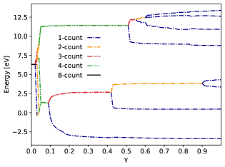
Figure 1: Degeneracy pattern of the average energy $\langle\tilde{h}\rangle$ of the DLWFs in silicon against $\gamma$ from Eq. (6). The color and line type indicate the degeneracy of the DLWFs; we call $\lvert w_{m}\rangle$ and $\lvert w_{n}\rangle$ degenerate if $|\langle\tilde{h}\rangle_{n}-\langle\tilde{h}\rangle_{m}|<$0.15\text{\,}\mathrm{eV}$$. At $\gamma=0$ (MLWFs), we obtain degenerate $sp^{3}$ hybrid orbitals, with each MLWF having occupancy $\lambda_{nn}=0.5$ and $\langle h\rangle=6.3$ eV. In the range $0.02<\gamma<0.05$, the DLWF degeneracy pattern rapidly changes before splitting into two degenerate sets between $0.05\leq\gamma\leq 0.09$: the occupied and unoccupied orbitals. The degeneracy of unoccupied DLWFs is lifted at $\gamma=0.53$, while the first lifting of degeneracy for occupied DLWFs occurs at $\gamma=0.1$.

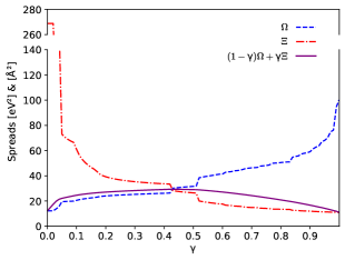
Figure 2: Spatial cost $\Omega$, energy cost $\Xi$, and total cost $F$ against $\gamma$ in Eq. (6). Since the total cost is a convex sum of $\Omega$ and $\Xi$, it always remains between their two values. The sharp changes in $\Omega$ and $\Xi$ correspond to degeneracy splitting in Fig. 1. Note the discontinuity in the vertical axis.

III.1.3 Converged frontier states

Next, we show convergence results when higher-energy virtual bands are included. For this result, we find that the spatial variance of the highest-energy occupied DLWF is well converged when 34 bands are disentangled to 30. Notably, we find that the shapes of the resulting DLWFs are qualitatively the same as those found when including only occupied orbitals (frontier orbitals), as in Sec. III.1.1 (Sec. III.1.2). We note, however, that the spatial variance $\Delta r^{2}$ of the lowest unoccupied DLWFs is larger than when only four unoccupied bands are included. This is due to the fact that the disentanglement in the latter case directly modifies the conduction bands, smoothing them in $\mathbf{k}$-space and unphysically increasing the localization of the resulting Wannier functions. Including more virtual orbitals in the localization procedure means that disentanglement smooths only the high-energy conduction bands, removing this effect. For isosurface plots of the eight lowest-energy DLWF densities, see Fig. 3. For more data on individual DLWFs, see the Supplemental Material.

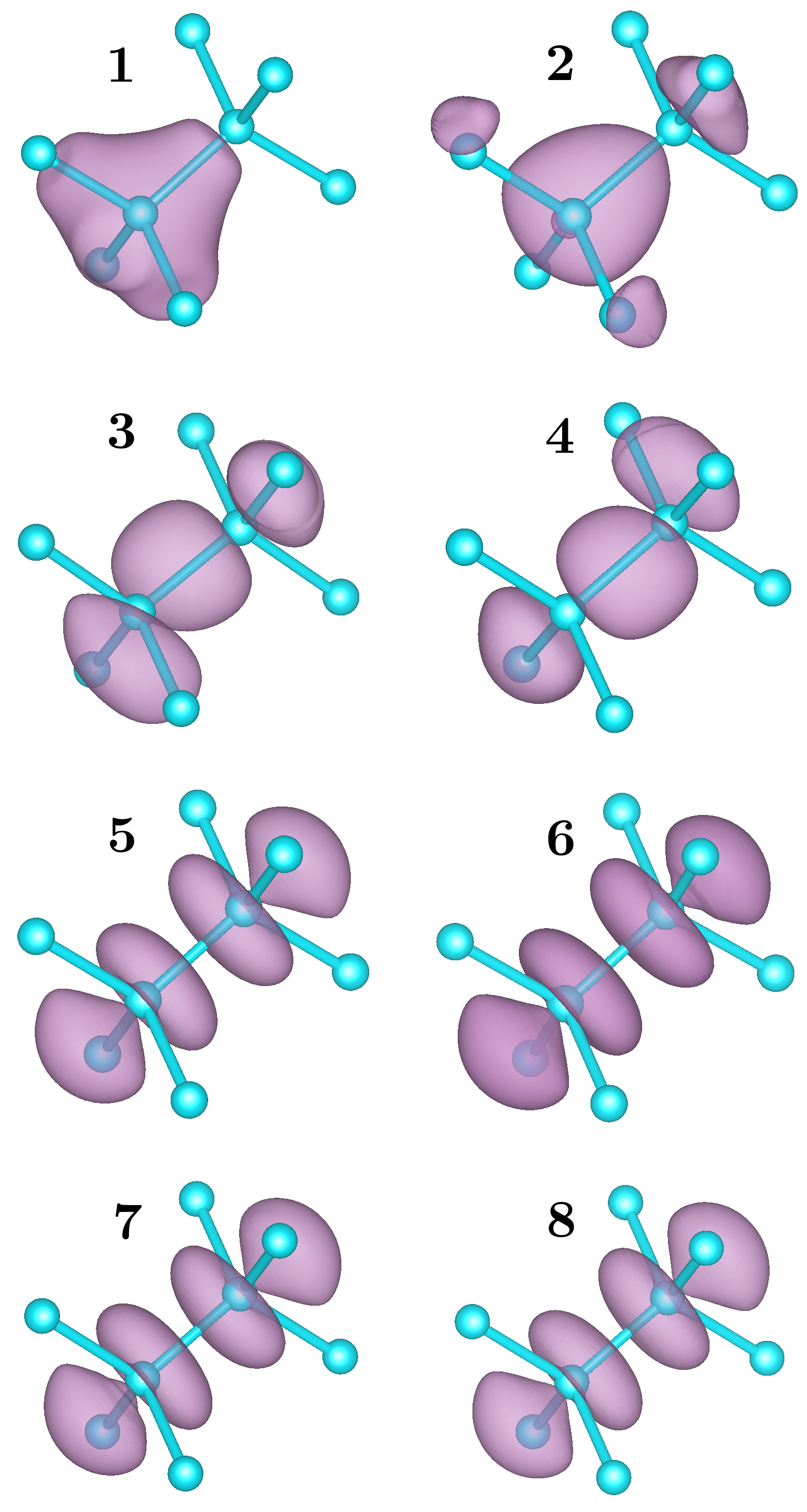
Figure 3: DLWF density isoplots for silicon (isovalue $0.6$) using $\gamma=0.47714$. They are labeled in ascending order of DLWF average energy starting at the lowest energy. Note that even though this is the result of using 30 disentangled Bloch orbitals per $\mathbf{k}$-point for construction, the degeneracy pattern is the same as the frontier-only case show in Fig. 1 for the value of $\gamma=0.47714$.

III.2 Copper

We next investigate copper in an face-centered cubic lattice using an experimental lattice parameter of $3.614\text{\,}\mathrm{\SIUnitSymbolAngstrom}$ [40]. For the self-consistent calculation we use a 16$\times$16$\times$16 $bk$-mesh, while for the virtual states and localization we use a 10$\times$10$\times$10 $\mathbf{k}$-mesh. Since the unoccupied bands of copper are very steep, and energy localization restricts mixing bands far apart in energy, we do not require many bands above the Fermi level. Noting that there are 9.5 electrons per spin channel, we use 23 bands and disentangle to 17 bands with a frozen disentanglement window of $40\text{\,}\mathrm{eV}$, well above the Fermi energy ($17.04\text{\,}\mathrm{eV}$). This results in a set of disentangled bands that only differs from the parent DFA at the top of the energy window. Using the $\gamma=0.47714$, we find that the fully occupied orbitals self-organize into pure $s$, $p$, and $d$-type DLWFs (see Fig. 4). The partially occupied DLWF associated with the frontier band has $d$-type character, but is delocalized across multiple atoms. Information on individual DLWFs is provided in the Supplemental Material.

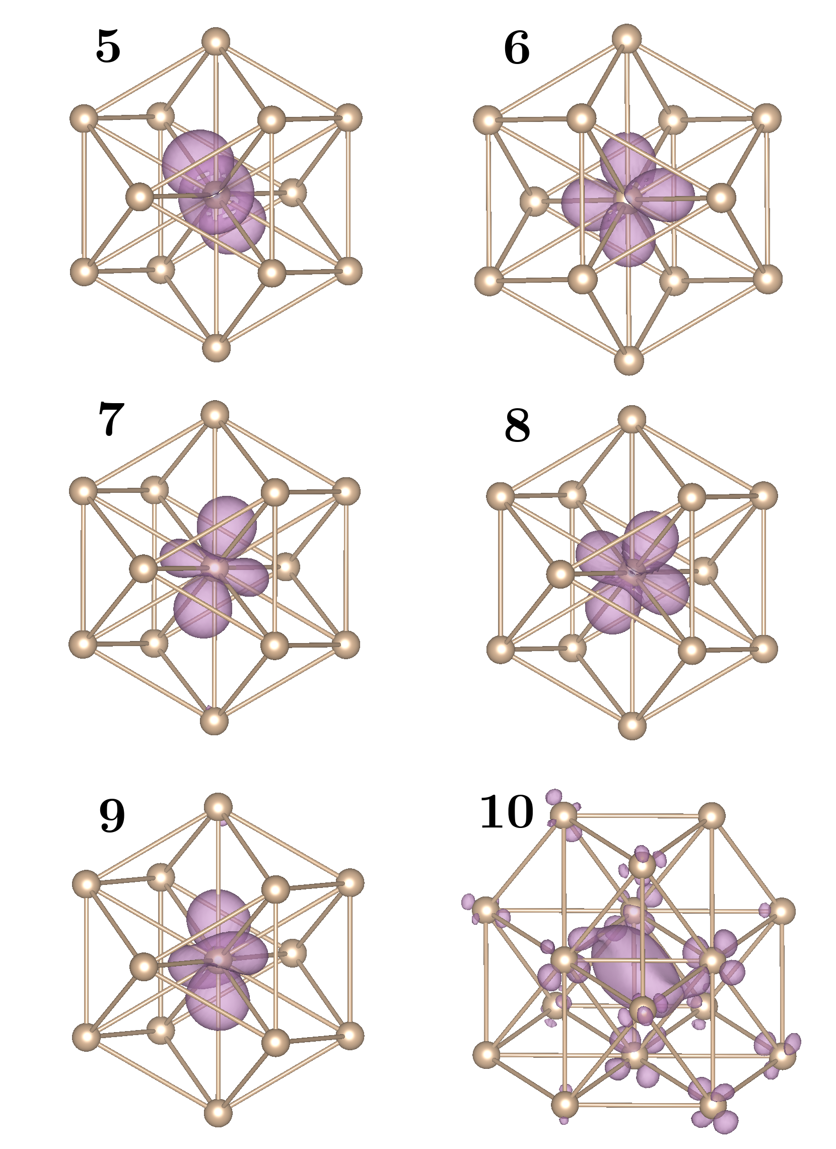
Figure 4: DLWF density isoplots of copper at isovalue $0.6$ using $\gamma=0.47714$. These are the six highest-energy occupied DLWFs labeled in ascending order of average energy, starting with the fifth-lowest energy. The four DLWFs of lowest energy (not shown) correspond to the occupied $3s$ and $3p$ states (not shown). DLWF 10 is only partially occupied, as it is mainly comprised of the frontier Bloch band. More atoms are shown for the isoplot of DLWF 10 due to its delocalized nature.

III.3 Ethylene

To demonstrate the utility of dual localization in molecules, we simulate ethylene with the geometry from [9]. We use a $10\text{\,}\mathrm{\SIUnitSymbolAngstrom}$ unit cell with the molecule centered at the origin and sample only the $\Gamma$. Thus, disentanglement is unnecessary, and we construct 36 DLWFs from 36 bands, 6 of which are occupied. Setting $\gamma=0.47714$ recovers DLWFs closely related to molecular orbitals. The lowest-energy DLWF corresponds to a $\sigma$ bond between the carbon atoms, and the next four resemble combinations of C–C and C–H bonding orbitals. The highest-energy occupied DLWF corresponds to a $\pi$ bonding orbital, and the lowest unoccupied DLWF to a $\pi^{*}$ antibonding orbital. Their isoplots are shown in Fig. 5, and the individual DLWF data are in the Supplemental Material.

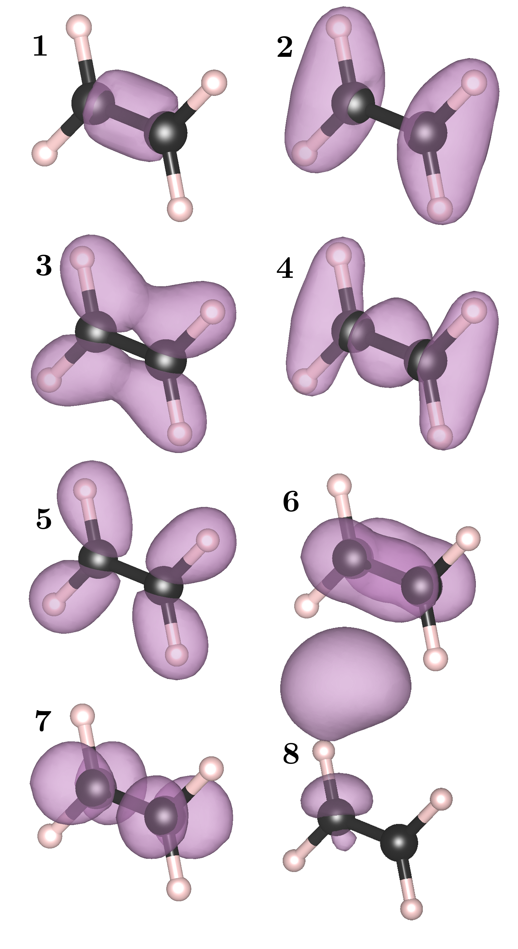
Figure 5: DLWF density isoplots for ethylene using $\gamma=0.47714$. DLWF 1 uses an isovalue of 160, DLWF 2–DLWF 7 use an isovalue of 60, and DLWF 8 uses an isovalue of 30. The isosurface between DLWF 6 and DLWF 8 belongs to DLWF 8.

IV Discussion

We have shown that including energy localization in the construction of Wannier functions results in DLWFs localized both in space and in energy. This allows for bands widely separated in energy to be included in the Wannier function construction without allowing the unphysical mixing of bands far apart in energy; furthermore, the localization procedure naturally produces orbitals associated with certain energies, organizing itself along the Hamiltonian’s spectrum. DLWFs with occupation close to $1$ also retain the behavior seen in MLWFs, appearing as tight-binding or atomic orbitals and retaining the symmetry of the underlying system. Using the LOSC cost function, $\gamma=0.47714$, the localization identifies atomic states such as the $d$ orbitals of copper (figure 4). The LOSC cost function also recovers molecular orbitals such as the ethylene $\sigma$ and $\pi$ bonding orbitals in Fig. 5. This shows that DLWFs have the potential to produce chemically relevant frontier orbitals automatically, without the need for manually enforced energy cutoffs or for separating the occupied and unoccupied spaces.

The fact that DLWFs offer a frontier orbital description localized in space means that they can be employed for orbital-dependent DFT methods [11, 12, 13, 14, 23]. Many of these methods attempt to correct the well-known failure of density functional approximations to give energy piecewise linear in fractional occupation [41]. In order to correct this nonlinear behavior, many of these corrections invoke localized frontier orbitals. A popular choice for these orbitals is to use MLWFs constructed from the highest-energy composite set of occupied Bloch bands. The fractional occupations in DLWFs are a key features distingushing them from other Wannier functions, and play an important role in the LOSC correction to density functional approximations [24, 23]. As DLWFs are explicitly associated with an energy level, they offer a localized charge description of frontier orbitals for both the occupied and unoccupied spaces. This means they can also generate relevant Wannier functions for both occupied and unoccupied frontier orbitals without having to localize each separately.

When the Wannier function construction includes entangled bands, Damle and Lin [42] have questioned whether sequential disentanglement and localization can find the globally optimal solution as separate procedures. The unified localization method proposed therein offers a possible solution to this problem. For a composite set of bands, this method reduces to the selected columns of the density matrix method [43, 44]; in that case, as with the original MLWF construction, energy cutoffs can be enforced explicitly to limit the energy spread of the Wannier functions. However, because the unified method of Damle and coworkers relies on the exponential decay of off-diagonal elements of the one-particle density matrix in space, it is unclear whether it can be adapted to include energy localization in the construction of the Wannier functions while allowing the inclusion of Bloch orbitals widely separated in energy, as shown in this work.

Finally, we comment on the (lack of) reality of the DLWFs. When $\gamma=0$, so that $F=\Omega$ in Eq. (6), Marzari and Vanderbilt conjectured in [9] that the resulting maximally localized Wannier functions would be purely real (up to a global phase). This was proven in [21] for Wannier functions constructed by minimizing any functional symmetric under time reversal, provided that the optimum is unique. Our cost function $F$ obeys time-reversal symmetry, and numerical tests show that the DLWFs with an occupation of $1$ are real. However, we observe substantial imaginary character in DLWFs that have an occupation numerically distinguishable from $1$. Even though the arguments in [21] do not differentiate between the occupied and unoccupied spaces, we conjecture that the reality arguments do not apply to Wannier functions whose occupation is far from 1. It is possible that the non-uniqueness of these minima could account for their lack of reality.

V Acknowledgements

All of the authors acknowledge support from the National Science Foundation (Grant No. CHE-1900338); A.M. from the Molecular Sciences Software Institute Phase-II Software Fellowship; and J.Z.W. from the National Institutes of Health (Grant No. 5R01GM061870).

References

- Wannier [1937] G. Wannier, Physical Review 52, 191 (1937).
- Silvestrelli and Parrinello [1999a] P. L. Silvestrelli and M. Parrinello, Phys. Rev. Lett. 82, 3308 (1999a), publisher: American Physical Society.
- Silvestrelli and Parrinello [1999b] P. L. Silvestrelli and M. Parrinello, The Journal of Chemical Physics 111, 3572 (1999b), publisher: American Institute of PhysicsAIP.
- Lee et al. [2005] Y.-S. Lee, M. B. Nardelli, and N. Marzari, Phys. Rev. Lett. 95, 076804 (2005), publisher: American Physical Society.
- Li and Marzari [2011] E. Y. Li and N. Marzari, ACS Nano 5, 9726 (2011), publisher: American Chemical Society.
- Shelley et al. [2011] M. Shelley, N. Poilvert, A. A. Mostofi, and N. Marzari, Computer Physics Communications 182, 2174 (2011).
- Goedecker [1999] S. Goedecker, Rev. Mod. Phys. 71, 1085 (1999).
- Souza et al. [2001] I. Souza, N. Marzari, and D. Vanderbilt, Phys. Rev. B 65, 035109 (2001), publisher: American Physical Society.
- Marzari and Vanderbilt [1997] N. Marzari and D. Vanderbilt, Phys. Rev. B 56, 12847 (1997), publisher: American Physical Society.
- Resta [2000] R. Resta, Berry’s phase and geometric quantum distance (2000), publisher: EPFL. Lausanne.
- Stengel and Spaldin [2008] M. Stengel and N. A. Spaldin, Phys. Rev. B 77, 155106 (2008), publisher: American Physical Society.
- Borghi et al. [2014] G. Borghi, A. Ferretti, N. L. Nguyen, I. Dabo, and N. Marzari, Phys. Rev. B 90, 075135 (2014), publisher: American Physical Society.
- Ma and Wang [2016] J. Ma and L.-W. Wang, Sci Rep 6, 24924 (2016).
- Wing et al. [2020] D. Wing, G. Ohad, J. B. Haber, M. R. Filip, S. E. Gant, J. B. Neaton, and L. Kronik, arXiv:2012.03278 [cond-mat] (2020), arXiv: 2012.03278.
- Monkhorst and Pack [1976] H. J. Monkhorst and J. D. Pack, Phys. Rev. B 13, 5188 (1976).
- Ashcroft and Mermin [2003] N. Ashcroft and D. Mermin, Solid State Physics (Thomson Press, 2003).
- Cloizeaux [1964] J. D. Cloizeaux, Phys. Rev. 135, A685 (1964).
- Cloizeaux [1963] J. D. Cloizeaux, Phys. Rev. 129, 554 (1963), publisher: American Physical Society.
- Foster and Boys [1960] J. M. Foster and S. F. Boys, Rev. Mod. Phys. 32, 300 (1960), publisher: American Physical Society.
- Kohn [1959] W. Kohn, Phys. Rev. 115, 809 (1959).
- Brouder et al. [2007] C. Brouder, G. Panati, M. Calandra, C. Mourougane, and N. Marzari, Phys. Rev. Lett. 98, 046402 (2007), publisher: American Physical Society.
- Panati and Pisante [2013] G. Panati and A. Pisante, Commun. Math. Phys. 322, 835 (2013).
- Su et al. [2020] N. Q. Su, A. Mahler, and W. Yang, J. Phys. Chem. Lett. 11, 1528 (2020).
- Li et al. [2018] C. Li, X. Zheng, N. Q. Su, and W. Yang, National Science Review 5, 203 (2018).
- Gygi et al. [2003] F. Gygi, J.-L. Fattebert, and E. Schwegler, Computer Physics Communications 155, 1 (2003).
- Daubechies [1992] I. Daubechies, Ten Lectures on Wavelets, CBMS-NSF Regional Conference Series in Applied Mathematics (Society for Industrial and Applied Mathematics, 1992).
- Mostofi et al. [2008] A. A. Mostofi, J. R. Yates, Y.-S. Lee, I. Souza, D. Vanderbilt, and N. Marzari, Computer Physics Communications 178, 685 (2008).
- Mostofi et al. [2014] A. A. Mostofi, J. R. Yates, G. Pizzi, Y.-S. Lee, I. Souza, D. Vanderbilt, and N. Marzari, Computer Physics Communications 185, 2309 (2014).
- Pizzi et al. [2020] G. Pizzi, V. Vitale, R. Arita, S. Blügel, F. Freimuth, G. Géranton, M. Gibertini, D. Gresch, C. Johnson, T. Koretsune, J. Ibañez-Azpiroz, H. Lee, J.-M. Lihm, D. Marchand, A. Marrazzo, Y. Mokrousov, J. I. Mustafa, Y. Nohara, Y. Nomura, L. Paulatto, S. Poncé, T. Ponweiser, J. Qiao, F. Thöle, S. S. Tsirkin, M. Wierzbowska, N. Marzari, D. Vanderbilt, I. Souza, A. A. Mostofi, and J. R. Yates, J. Phys.: Condens. Matter 32, 165902 (2020).
- Polak and Ribiere [1969] E. Polak and G. Ribiere, R.I.R.O. 3, 35 (1969).
- Fletcher and Reeves [1964] R. Fletcher and C. M. Reeves, The Computer Journal 7, 149 (1964).
- Press et al. [1992] W. Press, S. Taukolsky, W. Vetterling, and B. Flannery, Numerical Recipes in Fotran, The Art of Scientific Computing, 2nd ed. (Cambridge University Press, 1992).
- [33] github.com/mtesseracted/wannier90/tree/costSE.
- Perdew et al. [1996] J. P. Perdew, K. Burke, and M. Ernzerhof, Phys. Rev. Lett. 77, 3865 (1996).
- Hamann [2013] D. R. Hamann, Phys. Rev. B 88, 085117 (2013).
- van Setten et al. [2018] M. J. van Setten, M. Giantomassi, E. Bousquet, M. J. Verstraete, D. R. Hamann, X. Gonze, and G. M. Rignanese, Computer Physics Communications 226, 39 (2018).
- Giannozzi et al. [2009] P. Giannozzi, S. Baroni, N. Bonini, M. Calandra, R. Car, C. Cavazzoni, D. Ceresoli, G. L. Chiarotti, M. Cococcioni, I. Dabo, A. D. Corso, S. d. Gironcoli, S. Fabris, G. Fratesi, R. Gebauer, U. Gerstmann, C. Gougoussis, A. Kokalj, M. Lazzeri, L. Martin-Samos, N. Marzari, F. Mauri, R. Mazzarello, S. Paolini, A. Pasquarello, L. Paulatto, C. Sbraccia, S. Scandolo, G. Sclauzero, A. P. Seitsonen, A. Smogunov, P. Umari, and R. M. Wentzcovitch, J. Phys.: Condens. Matter 21, 395502 (2009), publisher: IOP Publishing.
- Giannozzi et al. [2017] P. Giannozzi, O. Andreussi, T. Brumme, O. Bunau, M. B. Nardelli, M. Calandra, R. Car, C. Cavazzoni, D. Ceresoli, M. Cococcioni, N. Colonna, I. Carnimeo, A. D. Corso, S. d. Gironcoli, P. Delugas, R. A. DiStasio, A. Ferretti, A. Floris, G. Fratesi, G. Fugallo, R. Gebauer, U. Gerstmann, F. Giustino, T. Gorni, J. Jia, M. Kawamura, H.-Y. Ko, A. Kokalj, E. Küçükbenli, M. Lazzeri, M. Marsili, N. Marzari, F. Mauri, N. L. Nguyen, H.-V. Nguyen, A. Otero-de-la Roza, L. Paulatto, S. Poncé, D. Rocca, R. Sabatini, B. Santra, M. Schlipf, A. P. Seitsonen, A. Smogunov, I. Timrov, T. Thonhauser, P. Umari, N. Vast, X. Wu, and S. Baroni, J. Phys.: Condens. Matter 29, 465901 (2017), publisher: IOP Publishing.
- Hom et al. [1975] T. Hom, W. Kiszenik, and B. Post, J Appl Crystallogr 8, 457 (1975).
- Rutt et al. [2006] O. J. Rutt, G. R. Williams, and S. J. Clarke, Chem. Commun. , 2869 (2006).
- Perdew et al. [1982] J. P. Perdew, R. G. Parr, M. Levy, and J. L. Balduz, PHYSICAL REVIEW LETTERS 49, 4 (1982).
- Damle and Lin [2018] A. Damle and L. Lin, Multiscale Model. Simul. 16, 1392 (2018).
- Damle et al. [2015] A. Damle, L. Lin, and L. Ying, J. Chem. Theory Comput. 11, 1463 (2015).
- Damle et al. [2017] A. Damle, L. Lin, and L. Ying, Journal of Computational Physics 334, 1 (2017).