Interplay of hyperbolic plasmons and superconductivity

Abstract

Hyperbolic plasmons are collective electron excitations in layered conductors. They are of relevance to a number of superconducting materials, including the cuprates and layered hyperbolic metamaterials [V. N. Smolyaninova, et al. Scientific Reports 6, 34140 (2016)]. This work studies how the unusual dispersion of hyperbolic plasmons affects Cooped pairing. We use the Migdal-Eliashberg equations, which are solved both numerically and analytically using the Grabowski-Sham approximation, with consistent results. We do not find evidence for plasmon-mediated pairing within a reasonable parameter range. However, it is shown that the hyperbolic plasmons can significantly reduce the effects of Coulomb repulsion in the Cooper channel leading to an enhancement of the transition temperature originating from other pairing mechanisms. In the model of a hyperbolic material composed of identical layers, we find this enhancement to be the strongest in the $d$-wave channel. We also discuss strategies for engineering an optimal hyperbolic plasmon background for a further enhancement of superconductivity in both $s$-wave and $d$-wave channels.

I Introduction

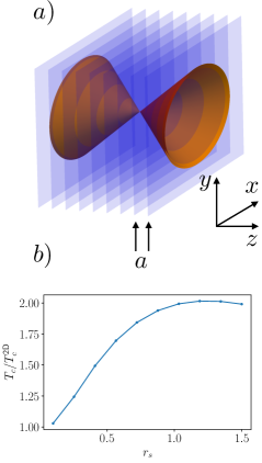
Figure 1: Superconductivity in a layered electron gas. a) Sketch of the setup: layered electron gas with inter-layer distance $a$. Hyperbolic plasmon dispersion is shown in orange. b) Enhancement of superconductivity in a $d$-wave channel: coupling constant $\mu^{*}$ as function of the Wigner-Seitz parameter $r_{s}$. The ratio between the superconducting transition temperatures in the layered electron gas and the 2DEG. The additional pairing interaction parameters are chosen as $\lambda=0.5$, $\omega_{0}=0.1E_{F}$. The interlayer distance $a=q_{0}^{-1}$ corresponds to the inverse of the Thomas-Fermi screening vector.

Plasmons are collective excitations of conducting electrons (Basov et al., 2021). In strongly anisotropic conductors, the plasmon dispersion is hyperbolic and can strongly modify the electromagnetic properties of such materials (Shekhar et al., 2014; Hawrylak et al., 1988). Some examples include the possibility of engineering a negative refraction index and lensing (Poddubny et al., 2013) beyond the diffraction limit (Smolyaninov, 2018). Hyperbolic materials were also proposed to enable long-range dipole-dipole interactions (Cortes and Jacob, 2017), which is potentially useful for efficient quantum information processing and transfer.

Hyperbolic plasmons in layered metals (Das Sarma and Quinn, 1982; Jain and Das Sarma, 1987) have the density of states, which is linear in energy, as was theoretically shown in (Morawitz et al., 1993). As a result, such plasmons are expected to strongly influence superconducting properties of hyperbolic materials. The effect of layering on superconductivity has been theoretically studied in a simplified way in Refs. (Kresin and Morawitz, 1988; Bill et al., 2003), where it was argued that the layering can increase the transition temperature.

The possibility of superconductivity mediated by two- and three-dimensional bulk plasmons was first theoretically considered in the early works by Takada (Takada, 1978, 1992) within the so-called Kirzhnits-Maksimov-Khomskii (KMK) Kirzhnits et al. (1973) approximation of the Migdal-Eliashberg equations. In particular, it was suggested that pairing can occur at low charge carrier densities. However, it was later realized (and we confirm this conclusion here) that the KMK approximation is not reliable. In particular, it underestimates the transition temperature (Schuh and Sham, 1983; Khan and Allen, 1980) in the case of the phonon-induced superconductivity and also fails to correctly describe the plasmonic mechanism of Cooper pairing Rietschel and Sham (1983).

The proper treatment of the plasmon-induced and plasmon-assisted pairing requires the use of full Migdal-Eliashberg equations (Grabowski and Sham, 1984), which is the focus of this paper, where we focus on layered materials. This research is partially motivated by recent experimental works (Smolyaninova et al., 2016, 2014), which demonstrated a strong enhancement of superconductivity in meta-materials with epsilon-near-zero (ENZ) properties (Liberal and Engheta, 2017; Smolyaninov, 2018). In particular, this has been achieved in a layered structure composed of conducting aluminium layers separated by thin dielectric layers of aluminium oxide. Due to the strong anisotropy of such materials, the plasmon spectrum is hyperbolic with the dielectric constant approaching zero along a set of cones in the phase space, as schematically shown in Fig. 1 (a). Based on the KMK arguments in (Smolyaninova et al., 2016, 2014) the authors directly attribute the observed increased critical temperature to the plasmon-induced mechanism of pairing. In the current work by solving the Migdal-Eliashberg equations we rule out the possibility of the superconductivity induced by hyperbolic plasmons only. Therefore the enhancement of the critical temperature in (Smolyaninova et al., 2016, 2014) must be explained by other mechanisms e.g. hyperbolic phonons, which will be considered elsewhere. However, we find here that hyperbolic plasmons in combination with an additional intrinsic attractive interaction can lead to an enhancement of pairing.

In this work we perform a systematic study of the effect of hyperbolic plasmons on superconductivity. We consider both pairing due to plasmon mechanism and a hyperbolic plasmon-assisted pairing on top of another intrinsic pairing mechanism, e.g., due to phonons or magnons. Within the Random Phase Approximation (RPA) we numerically solve the complete set of Migdal-Eliashberg equations (Marsiglio, 2020), and as shown in Fig. 1 (b), find a significant enhancement of superconductivity in the $d$-wave channel and in the presence of additional attractive pairing mechanism in the corresponding channel. The latter may be of relevance to high-temperature superconductivity in cuprates Tsuei and Kirtley (2000). In order to get a qualitative insight into our numerical solution, we employ the Grabowski-Sham approximation (Grabowski and Sham, 1984) and consider the band-averaged electron-electron interaction. We find that the effect of hyperbolic plasmons on the transition temperature is two-fold. On the one hand, they screen the Coulomb repulsion more efficiently compared to the conventional two-dimensional plasmons. On the other, they have a larger effective screening energy range. These two effects are found to compete in how they impact the superconducting transition temperature. We also consider the possibility of engineering (Little, 1964) a plasmon structure of layered materials to optimize the enhancement effect on superconductivity. One proposed proof-of-principle scenario involves a layered structure, where one of the layers is distinct from the other identical layers. We demonstrate a possible significant enhancement of the superconducting transition temperature in such a configuration in both $s$-wave and $d$-wave channels.

This paper is structured as follows: Sec. II introduces the Migdal-Eliashberg formalism that takes into account retardation effects. In Sec. III, we solve the Migdal-Eliashberg equations numerically for pure Coulomb interaction in the layered electron gas. To elucidate the numerical results, in Sec. IV we introduce several approximation schemes that allow us to provide an intuitive picture of the hyperbolic plasmon-mediated pairing. In Sec. V, we consider the effect of hyperbolic plasmons on other pairing mechanisms and demonstrate a possible enhancement of pairing the $d$-wave channel. Sec. V.2 provides an example of a setup for the further enhancement of pairing by engineering the plasmon dispersion in a hyperbolic/layered structure.

II Formulation

We consider a layered electron gas with the inter-layer spacing $a$ (see, Fig. 1) Das Sarma and Quinn (1982), which can be either a meta-material structure Smolyaninov (2018) or a layered compound (e.g., a cuprate material). We describe electron properties of each layer by a Coulomb-interacting 2-dimensional electron gas (2DEG) model. The full Hamiltonian reads:

$$\hat{H}_{\text{full}} =\hat{H}_{0}+\hat{H}_{\text{int}},$$ (1)

$$\hat{H}_{0} =\sum_{i,{\bf k},\sigma}\xi_{k}\hat{\psi}_{{\bf k},\sigma}^{\left(i\right)\dagger}\hat{\psi}_{{\bf k},\sigma}^{\left(i\right)},$$ (2)

$$\hat{H}_{\text{int}} =\frac{1}{2A}\sum_{i\leq j,{\bf k,k^{\prime},q},\sigma,\sigma^{\prime}}\tilde{V}_{{\bf q}}^{\left(i,j\right)}\hat{\psi}_{{\bf k}+{\bf k},\sigma}^{(i)\dagger}\hat{\psi}_{{\bf k}^{\prime}-{\bf q},\sigma^{\prime}}^{(j)\dagger}\hat{\psi}_{{\bf k}^{\prime},\sigma^{\prime}}^{(j)}\hat{\psi}_{{\bf k},\sigma}^{(i)},$$ (3)

where $\hat{\psi}_{{\bf k},\sigma}^{\left(i\right)}$ denotes the creation/annihilation operator of spin-$\sigma$ electron on $i$-th layer. $\xi_{k}=k^{2}/2m-E_{F}$ where $m$ refers to the bare electron mass, $A$ is the surface area of each layer and $E_{F}$ is the Fermi energy. $\tilde{{\cal V}}_{{\bf q}}^{\left(i,j\right)}=2\pi e^{2}e^{-aq\left|i-j\right|}/\epsilon_{\infty}q$ denotes the bare Coulomb interaction of electrons on $i$-th and $j$-th layers, $a$ denotes the interlayer distance and $\epsilon_{\infty}$ is the background dielectric constant and $e$ is the electron charge. In the following ${\bf q}$ denotes the two-dimensional in-plane momentum. In our model Eq. (1) we neglected the electron tunnelling between layers. In Fourier space with respect to the layer index the bare Coulomb interaction is

$$\tilde{{\cal V}}_{{\bf q},q_{z}}=\frac{2\pi e^{2}}{\epsilon_{\infty}q}\frac{\sinh aq}{\cosh aq-\cos q_{z}},$$

where $q_{z}\in[-\pi,\pi]$ denotes the out-of-plane momentum. The conventional RPA-renormalized interaction reads:

$${\cal V}_{{\bf q},q_{z}}\left(i\Omega_{m}\right)=\frac{1}{\tilde{{\cal V}}_{{\bf q},q_{z}}^{-1}+\frac{m}{\pi}\Pi_{{\bf q}}\left(i\Omega_{m}\right)}$$ (4)

where $\Pi_{{\bf q}}$ is the polarization operator of the 2D electron gas normalized as $\Pi_{{\bf q}\rightarrow 0}\left(0\right)=1$ and $\Omega_{m}=2\pi m/\beta$.

$${\cal V}_{{\bf q},q_{z}}\left(i\Omega_{m}\right)=\frac{2\pi e^{2}}{\epsilon_{\infty}}\frac{1}{q\frac{\cosh aq-\cos q_{z}}{\sinh aq}+q_{0}\Pi_{{\bf q}}\left(i\Omega_{m}\right)},$$ (5)

where $q_{0}=2me^{2}/\epsilon_{\infty}$ denotes the Thomas-Fermi screening length. The latter characterizes the momentum-scale below which the interaction is efficiently screened.

Within the RPA the normal-state electron Green’s function has the following form:

$${\cal G}_{{\bf k}}\left(i\varepsilon_{n}\right) \equiv-\int_{0}^{\beta}e^{i\varepsilon_{n}\tau}\left\langle\hat{\psi}_{{\bf k,\sigma}}^{\left(i\right)}\left(\tau\right)\hat{\psi}_{{\bf k},\sigma}^{\left(i\right)\dagger}\left(0\right)\right\rangle$$

$$=\frac{1}{-\xi_{k}+i\varepsilon_{n}-\Sigma_{{\bf k}}\left(i\varepsilon_{n}\right)}$$ (6)

where $\varepsilon_{n}=\left(2n+1\right)\pi/\beta,n\in\mathbb{Z}$ and $\beta$ denotes the inverse temperature. As we assume all layers to be identical and neglect tunnelling between layers, the Green function in Eq. (6) is independent of the layer index. The normal state self-energy denoted above as $\Sigma_{{\bf k}}$ obeys the Dyson equation:

$$\Sigma_{{\bf k}}\left(i\varepsilon_{n}\right) =-\frac{1}{\beta A}\sum_{{\bf k^{\prime}},m}G_{{\bf k^{\prime}}}\left(i\varepsilon_{m}\right){\cal V}_{{\bf k}-{\bf k^{\prime}}}^{\left(i,i\right)}\left(i\varepsilon_{m}-i\varepsilon_{n}\right),$$ (7)

where ${\cal V}_{{\bf q}}^{(i,j)}(i\Omega_{m})=(2\pi)^{-1}\int dq_{z}e^{iq_{z}(i-j)}{\cal V}_{{\bf q},q_{z}}(i\Omega_{m})$ denotes the Fourier transform of the interaction Eq. (4). The superconducting anomalous self-energy on $i$-th layer obeys the following equation:

$$\phi_{{\bf k}}\left(i\varepsilon_{n}\right) =-\left(\beta A\right)^{-1}\sum_{{\bf k^{\prime}},m}{\cal V}^{(i,i)}_{{\bf k}-{\bf k^{\prime}}}\left(i\varepsilon_{n}-i\varepsilon_{m}\right)$$

$$\times{\cal G}_{{\bf k^{\prime}}}\left(i\varepsilon_{m}\right){\cal G}_{-{\bf k^{\prime}}}\left(-i\varepsilon_{m}\right)\phi_{{\bf k^{\prime}}}\left(i\varepsilon_{m}\right).$$ (8)

We solve this equation numerically for both pure Coulomb interaction and it co-existing with other pairing mechanisms. We also consider simplified analytical models for both cases, which help us develop an intuitive physical picture behind the numerical results.

II.1 Hypebolic plasmon dispersion

We now describe the plasmon structure of the layered electron gas defined above. For that we perform the analytic continuation of the Coulomb propagator to real-frequency:

$$\text{Im}V_{q,q_{z}}(\omega+i0^{+})=\frac{2\pi e^{2}}{\epsilon_{\infty}}\text{Im}\frac{1}{q\frac{\cosh aq-\cos q_{z}}{\sinh aq}+q_{0}\Pi_{q}\left(\omega\right)},$$ (9)

Its poles correspond to the collective excitations of the layered electron gas (plasmons). We readily find the long-wavelength plasmon excitation dispersion for $q_{z}\neq 0$:

$$\varepsilon_{q}=v_{F}\sqrt{1+\frac{aq_{0}}{2\sin^{2}(q_{z}/2)}}q,$$ (10)

where $v_{F}=k_{F}/m$ is the Fermi velocity. For $q_{z}=0$ the spectrum is gapped and the dispersion is $\varepsilon_{q\rightarrow 0}\approx v_{F}\sqrt{q_{0}/a}$. For any non-zero $q_{z}$ the fixed-frequency curves form cones in momentum space as schematically shown in Fig. 1 (a). The full plasmon spectrum is shown in Fig. 2. We note several features of the spectrum Eq. (10). First, it has a finite density of states at low energies. Second, it extends to higher frequencies compared to the pure two-dimensional plasmons.

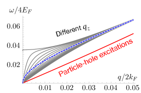
Figure 2: Layered plasmon spectrum for the interlayer spacing $a=1/q_{0}$. Different gray curves correspond to different values of $q_{z}\in\left[0,\pi\right]$ . Blue dashed line stands for the pure 2-dimensional plasmon spectrum. Red curve corresponds to the particle-hole excitation spectrum of the electron gas.

II.2 Angular averaging. Migdal-Eliashberg equations.

To solve Eq. (8), we first project the gap function onto a particular angular momentum eigenstate $\phi_{{\bf k}}\propto e^{il\vartheta}+c.c.$, where $\vartheta$ is the angular coordinate. For the sake of convenience below we express all energy and momentum variables in $4E_{F}$ and $2k_{F}$ respectively: $k\rightarrow 2k_{F}k$, $a\rightarrow a/2k_{F}$, $\beta\rightarrow\beta/4E_{F}$. In these units the normal-state Green function has the following form ${\cal G}_{k}^{-1}\left(i\varepsilon_{m}\right)=i\varepsilon_{m}-k^{2}+1/4-\Sigma_{\bf{k}}$.

Let us now explicitly consider the gap equation Eq. (8) in the $l$-wave channel. By transforming summations into integrals we readily find:

$$\phi_{{\bf k}}^{(l)}\left(i\varepsilon_{n}\right)= -T\sum_{n}\int k^{\prime}dk^{\prime}\int_{0}^{2\pi}\frac{d\vartheta}{2\pi}\int_{-\pi}^{\pi}\frac{dk_{z}}{2\pi}$$

$$\times\frac{q_{0}}{u\frac{\cosh au-\cos k_{z}}{\sinh au}+q_{0}\Pi_{u}}\frac{\phi_{{\bf k^{\prime}}}^{(l)}\left(i\varepsilon_{m}\right)}{\left|{\cal G}_{k^{\prime}}^{-1}\left(i\varepsilon_{m}\right)\right|^{2}},$$ (11)

where $u\equiv\left|{\bf k}-{\bf k^{\prime}}\right|=\sqrt{k^{2}+k^{\prime 2}-2kk^{\prime}\cos(\vartheta)}$. As we see from the expression the result depends only on two variables: $q_{0}$ and $a$. Now assuming a particular angular momentum $l$ of the gap we can perform the angular integral:

$$\phi_{k}^{(l)}\left(i\varepsilon_{n}\right)=-T\sum_{m}\int k^{\prime}dk^{\prime}{\cal V}_{k,k^{\prime}}^{(l)}\left(i\varepsilon_{n}-i\varepsilon_{m}\right)\frac{\phi_{{\bf k^{\prime}}}^{(l)}\left(i\varepsilon_{m}\right)}{\left|{\cal G}_{k^{\prime}}^{-1}\left(i\varepsilon_{m}\right)\right|^{2}},$$ (12)

where the angular-averaged interaction is defined as:

$${\cal V}_{k,k^{\prime}}^{(l)}\left(i\Omega_{n}\right)=\int\frac{d\vartheta}{2\pi}\int_{-\pi}^{\pi}\frac{dk_{z}}{2\pi}\frac{q_{0}\cos(\vartheta l)}{u\frac{\cosh au-\cos q_{z}}{\sinh au}+q_{0}\Pi_{u}}$$

$$=\int\frac{d\vartheta}{2\pi}\frac{q_{0}\sinh(au)\cos(\vartheta l)}{\sqrt{\left(u\cosh au+q_{0}\sinh au\Pi_{u}\left(i\Omega_{n}\right)\right)^{2}-u^{2}}}$$ (13)

We note that the propagator for the nearest-neighbor layers can also be found analytically. Analogously, we find the corresponding equation for the normal-state self-energy:

$$\Sigma_{k}\left(i\varepsilon_{n}\right) =-T\sum_{m}\int k^{\prime}dk^{\prime}{\cal V}_{k,k^{\prime}}^{(l=0)}\left(i\varepsilon_{m}-i\varepsilon_{n}\right){\cal G}_{k^{\prime}}\left(i\varepsilon_{m}\right).$$ (14)

We now define the conventional 2-dimensional Wigner-Seitz parameter $2\pi a_{\text{Bohr}}^{2}r_{s}^{2}n=1$, where $a_{\text{Bohr}}$ is the Bohr radius in dielectric with the polarizability $\epsilon_{\infty}$. $r_{s}$ can be expressed via the dimensionless Thomas-Fermi vector as $r_{s}=\sqrt{2}q_{0}$. In the following section we solve Eqs. (12, 14) numerically.

III Numerical solution of Migdal-Eliashberg equations

In this section we provide details of numerical solution of Migdal-Eliashberg equations Eqs. (12, 14). In Sec. III.1 we discuss the calculation of the normal-state self energy. We then numerically solve the gap equation for $s$- and $d$-wave pairing channels. We find that the plasmon induced pairing is impossible in the reasonable parameter range.

III.1 Normal state self-energy

The self-consistent solution of the gap equation in case of Coulomb interaction requires caution as the interaction kernel in Eqs. (12, 14) has a logarithmic singularity for $k=k^{\prime}$ (Rietschel and Sham, 1983). We therefore introduce a momentum grid which has density of momentum points with the smallest $\Delta k\propto 10^{-3}k_{F}$. We first solve Eq. (14) iteratively. As we explain in more detail below, it is convenient to make the conventional variable change (Rietschel and Sham, 1983):

$$\chi_{k}\left(i\varepsilon_{n}\right)= \frac{\Sigma_{k}\left(i\varepsilon_{n}\right)+\Sigma_{k}\left(-i\varepsilon_{n}\right)}{2},$$ (15)

$$Z_{k}\left(i\varepsilon_{n}\right)= 1+i\frac{\Sigma_{k}\left(i\varepsilon_{n}\right)-\Sigma_{k}\left(-i\varepsilon_{n}\right)}{2\varepsilon_{n}},$$ (16)

where from Eq. (14) $Z_{k}\left(i\varepsilon_{n}\right)$ is found to obey:

$$\varepsilon_{n}\left(Z_{k}\left(i\varepsilon_{n}\right)-1\right)=$$

$$T\int k^{\prime}dk^{\prime}\sum_{m}\frac{\varepsilon_{m}Z_{k^{\prime}}\left(i\varepsilon_{m}\right)}{\left|{\cal G}_{k^{\prime}}^{-1}\left(i\varepsilon_{m}\right)\right|^{2}}{\cal V}_{k,k^{\prime}}^{(l=0)}\left(i\varepsilon_{m}-i\varepsilon_{n}\right),$$ (17)

The even-frequency part of the normal-state self-energy $\chi_{k}\left(i\varepsilon_{n}\right)$ function has static and dynamical contributions:

$$\chi_{k}\left(i\varepsilon_{n}\right) =\chi_{k}^{\left(0\right)}+\chi_{k}^{\left(1\right)}\left(i\varepsilon_{n}\right)$$ (18)

$$\chi_{k}^{\left(0\right)} =-T\int k^{\prime}dk^{\prime}\sum_{m}\frac{\xi_{k^{\prime}}+\chi_{k^{\prime}}\left(i\varepsilon_{m}\right)}{\left|{\cal G}_{k^{\prime}}^{-1}\left(i\varepsilon_{m}\right)\right|^{2}}{\cal\tilde{V}}_{k,k^{\prime}},$$ (19)

$$\chi_{k}^{\left(1\right)}\left(i\varepsilon_{n}\right) =-T\int k^{\prime}dk^{\prime}\sum_{m}\frac{\xi_{k^{\prime}}+\chi_{k^{\prime}}\left(i\varepsilon_{m}\right)}{\left|{\cal G}_{k^{\prime}}^{-1}\left(i\varepsilon_{m}\right)\right|^{2}}\delta{\cal V}_{k,k^{\prime}}^{(l=0)}\left(i\varepsilon_{m}-i\varepsilon_{n}\right)$$ (20)

where ${\cal\tilde{V}}_{k,k^{\prime}}$ refers to the bare unrenormalized Coulomb interaction and $\delta{\cal V}_{k,k^{\prime}}^{(l)}\equiv{\cal V}_{k,k^{\prime}}^{(l=0)}-{\cal\tilde{V}}_{k,k^{\prime}}$. The advantage of this representation is that $\chi_{k}^{\left(0\right)}$ is frequency-independent while $\chi_{k}^{\left(1\right)}$ has finite frequency range and can be solved by introducing a frequency cut-off. Equations for $\chi$ and $Z$ can be solved iteratively starting with some initial value (Rietschel and Sham, 1983).

III.2 Numerical procedure

For solution of Eqs. (12), we note that the gap function is frequency-dependent and does not vanish at large frequencies:

$$\phi_{k}^{\left(i,j\right)}\left(\pm i\infty\right)=-T\sum_{m}\int k^{\prime}dk^{\prime}\frac{\phi_{k^{\prime}}^{\left(i,j\right)}\left(i\varepsilon_{m}\right)}{\left|{\cal G}_{k^{\prime}}^{-1}\left(i\varepsilon_{m}\right)\right|^{2}}{\cal\tilde{V}}_{k,k^{\prime}}.$$ (21)

This implies that we cannot impose a simple frequency cutoff in the integral equation. Here instead we introduce a cut-off, $\epsilon_{*}$, above which the gap function is assumed constant and reaches its infinite-frequency value $\phi_{k^{\prime}}^{(i,j)}(i|\varepsilon_{n}|>\varepsilon_{\epsilon_{*}})=\phi_{k^{\prime}}^{(i,j)}\left(i\infty\right)$. The value of $\epsilon_{*}$ is chosen to ensure the convergence of the iterative procedure and by the condition that a further increase of $\epsilon_{*}$ does not affect the transition temperature withing desired accuracy.

With the above in mind we now describe the iterative numerical procedure for solving Eqs. (12, 14). We start with the iterative procedure with the Green function for a free Fermi gas; i.e. $\Sigma^{(0)}_{k}=0$. Using the decomposition into odd- and even-frequency parts described in Sec. III.1, we numerically apply the integral operator on the right-hand side of Eq. (14) $n$ times and find $\Sigma^{(n)}_{k}$. It is typically sufficient to perform approximately 10 iterative steps until the difference $|\Sigma^{(n)}_{k}-\Sigma^{(n-1)}_{k}|\ll|\Sigma^{(n)}|$ is negligible and the iteration scheme converges. Once normal-state self energy is obtained we can solve the gap equation Eq. (12). A solution of this equation determines the critical temperature $T_{c}$. Equivalently, at the transition temperature the discretized integral operator on the right-hand side of Eq. (12) has eigenvalue 1.

We find the transition point by changing temperature as a parameter of the integral kernel.

III.3 Numerical results

We now discuss the results of the numerical solution of the gap equation Eq. (12) according to the procedure outlined above. In addition to the pure plasmon-induced superconductivity, we also consider the case when some additional attraction between electrons is present. For the latter case here we only describe the final result leaving most of the details to Sec. V.

At the electron densities corresponding to the regime of validity of the RPA, we find no possible plasmon-induced pairing in both layered and in the conventional 2-dimensional electron gas regime. While in agreement with the earlier studies (Takada, 1978),(Rietschel and Sham, 1983) the solution of Eliashberg equations exists for $r_{s}>r^{*}_{s}$, where $r^{*}_{s}\approx 2$, which is beyond the applicability of the RPA. In this case, it is important to keep vertex corrections which may qualitatively change the result. Extrapolating the results outside the RPA validity range we find that the layering is decreasing the transition temperature for $r_{s}>r^{*}_{s}$. The same behavior occurs in the $d$-wave channel as well. In conclusion, within the RPA we do not find a regime where plasmon-induced pairing is possible.

The situation is, however, different if we add an additional attractive interaction in the $d$-wave channel. More precisely, we consider the following modification of the Coulomb interaction Eq. (13):

$${\cal V}_{k,k^{\prime}}^{(l)}(i\Omega_{n})\rightarrow{\cal V}_{k,k^{\prime}}^{(l)}(i\Omega_{n})-\lambda\delta_{l,2}\frac{\omega_{0}^{2}}{\omega_{0}^{2}+\Omega_{n}^{2}},$$ (22)

where $\lambda$ is some effective interaction strength and $\omega_{0}$ is the characteristic frequency. We note that the additional interaction in Eq. (22) can be induced by a single-frequency bosonic mode. As shown in Fig. 1 (c), we find an enhancement of the transition temperature in a layered electron gas compared to the conventional 2-dimensional electron gas. We note that depending on the parameters the observed enhancement can be quite significant. In particular for our choice of parameters in Fig. 1 (c) the critical temperature is doubled at $r_{s}=1$. In the next section, we study a simplified model which, as we show, can explain all the features of the transition temperature.

IV Toy model of plasmon-mediated pairing

In this section, we discuss a toy model that reproduces the behavior of $T_{c}$ shown discussed above. The aim of this section is solely to develop an intuitive picture of the plasmon-mediated Cooper pairing. For that, we use a simplified model with no renormalization of the normal-state Green’s function. We start with Eq. (12):

$$\phi_{k}^{(l)}\left(i\varepsilon_{n}\right)=$$

$$-T\sum_{m}\int k^{\prime}dk^{\prime}{\cal V}_{k,k^{\prime}}^{(l)}\left(i\varepsilon_{m}-i\varepsilon_{n}\right)\frac{\phi_{k^{\prime}}^{(l)}\left(i\varepsilon_{m}\right)}{\varepsilon_{m}^{2}+\xi_{k^{\prime}}^{2}}.$$ (23)

To get an analytical insight we now reduce the complete 2-dimensional Migdal-Eliashberg equation (23) to an effective 1-D form. Due to the long-range nature of Coulomb interaction, we cannot perform the conventional Fermi-surface averaging of the interaction. Indeed, at high Matsubara frequencies we find:

$${\cal V}_{k_{F},k_{F}}^{(l)}\left(i\Omega_{n}\right)\propto\int_{0}^{2\pi}d\vartheta\frac{\cos(\vartheta l)}{\sqrt{1+\cos\vartheta}}.$$

The right-hand side of this integral logarithmically diverges at $\vartheta\sim\pi$ (Rietschel and Sham, 1983). This divergence is present for all frequencies except for the zeroth one. to circumvent this technical issue, we resort to the heuristic Grabowski-Sham approximation introduced in (Grabowski and Sham, 1984). Following their approach (with a slight modification that produces more accurate results in comparison with the brute-force numerical solution of the original integral equation), we replace the momentum-dependent interaction with:

$${\cal V}^{(l)}\left(i\Omega_{n}\right)\equiv\frac{\int kdk\theta\left(k_{\text{c}}-k\right){\cal V}_{k,k_{F}}^{(l)}\left(i\Omega_{n}\right)}{\int kdk\theta\left(k_{\text{c}}-k\right)},$$ (24)

where $\theta$ is the Heaviside theta-function and $k_{c}$ is the cut-off momentum chosen according to the bandwidth of the electron gas. Overall, we can conveniently parameterize (Grabowski and Sham, 1984) the interaction as follows:

$${\cal V}^{(l)}\left(i\varepsilon_{m}-i\varepsilon_{n}\right)\equiv\mu\left(1-\sigma v_{m,n}\right)$$ (25)

with $v_{m,n\rightarrow\infty}\rightarrow 0,v_{0,0}=1$ and $\sigma$ being a dimensionless coefficient, characterizing screening strength. A typical example of this function is shown in Fig. 3. Here we observe a suppression of the Coulomb interaction at Matsubara frequencies below some characteristic screening energy scale $\varepsilon_{\text{sc}}$. The latter can be heuristically inferred from the curves Fig. 3 by fitting $v_{m,n}$ with e.g. Lorentz curve (the result is shown in insets).

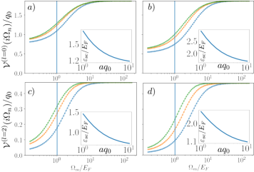
Figure 3: Effective interaction ${\cal V}(i\Omega_{n})$ Eq. (24) for $aq_{0}=1$ (blue), $aq_{0}\approx 3.2$ (orange) and $aq_{0}=10$ (green). $s$-wave channel with electron density is a) $r_{s}=0.8$, b) $r_{s}=1.5$. $d$-wave channel with electron density is c) $r_{s}=0.8$, d) $r_{s}=1.5$. Insets shows the effective screening energy $\varepsilon_{\text{sc}}$ as function of the inter-layer distance $a$. In both figures the blue vertical line corresponds to the Fermi energy.

Since we now ignore the momentum dependence of the interaction potential the gap equation simplifies to:

$$\phi^{(l)}\left(i\varepsilon_{n}\right)=-T\sum_{m}{\cal V}^{(l)}\left(i\varepsilon_{m}-i\varepsilon_{n}\right)\int\frac{\phi^{(l)}\left(i\varepsilon_{m}\right)d\xi_{k^{\prime}}}{\varepsilon_{m}^{2}+\xi_{k^{\prime}}^{2}}.$$ (26)

Eq. (25) is one-dimensional and therefore it is straightforward to solve numerically. It is however more practical to use the pseudo-potential method Grabowski and Sham (1984). It allows us to define the coupling strength even in the case when there is no superconductivity: $\mu^{*}<0$. In the latter case the quantity $-\mu^{*}$ is typically referred to as the Coulomb pseudopotential. The idea behind the pseudopotential method is to replace the long-range (in frequency) interaction in Eq. (26) with a short-range one. For the latter, the critical temperature can be found trivially as discussed in the SM. The superconducting coupling constant obtained from the approximation Eq. (25) is shown in Fig. 4. We observe that in the regime when $\mu^{*}$ is positive the layering is typically detrimental for the pairing in $s$- and $d$-wave channels. The only regime where layering is useful is in $d$-wave channel at $r_{s}\approx 1$.

IV.1 Analytical estimate of the transition temperature

In order to explain the properties of the plasmon-mediated Cooper pairing it is instructive to consider the exactly solvable model. More precisely, we assume a separable square-well model for the interaction: $v_{m,n}\approx\theta(\varepsilon_{\text{sc}}^{2}-\varepsilon_{m}^{2})\theta(\varepsilon_{\text{sc}}^{2}-\varepsilon_{n}^{2})$, where $\theta$ is the Heaviside theta-function. By inserting this ansatz to Eq. (26) in the limit $\varepsilon_{\text{sc}}\ll E_{F}$ the transition temperature is found to be (see Appendix A):

$$T_{c}=1.134E_{F}e^{-1/\mu^{*}}$$ (27)

with $\mu^{*}=-\log(E_{F}/\varepsilon_{\text{sc}})+\mu\left(\sigma-1/(1+\mu\log\frac{E_{F}}{\varepsilon_{\text{sc}}})\right)$. The condition on existence of the superconductivity is given by $\mu^{*}>0$. We also see the suppression of the overall Coulomb repulsion term by the logarithmic prefactor. From Eq. (27) we find the optimal value $\varepsilon_{\text{sc}}=e^{\left(\sigma-2\right)/\mu\sigma}E_{F}$ at which the critical temperature is maximal. At larger values the critical temperature is decreasing becoming exactly zero at $\varepsilon_{\text{sc}}=e^{\left(\sigma-1\right)/\mu\sigma}E_{F}$.

With the above in mind we now analyze the properties of the effective interaction ${\cal V}\left(i\Omega_{n}\right)$ shown in Fig. 3. The effect of layering is found to be two-fold: first it increases the screening strength, $\sigma$, and second, it increases the corresponding screening energy range $\varepsilon_{\text{sc}}$. As clear from Eq. (27), the two effects discussed above contribute to $T_{c}$ in the opposite way. Besides the negative effect is usually dominating. The only regime when the pairing is enhanced is found in the $d$-wave channel at smaller values $r_{s}<1$. This can be explained by the fact that the effective interaction has the lowest screening energy scale $\varepsilon_{\text{sc}}$ and the highest relative screening strength $\sigma$. We note that although $\mu^{*}$ is enhanced by layering, the Cooper pairing itself is not possible due to the overall sign of $\mu^{*}<0$. It therefore appears impossible to achieve a pure plasmon-induced superconductivity or an enhancement thereof by hyperbolic plasmons (unless we consider high $r_{s}$ values, where no reliable theoretical methods exist).

In conclusion of this section, we reiterate that the renormalization of the Coulomb pseudopotential by hyperbolic plasmons contain two competing factors: the enhancement of the plasmon-induced screening parameterized by $\sigma$ and the increase of the effective screening energy range, $\varepsilon_{\text{sc}}$. In the case of $d$-wave superconductivity, the microscopic details of the interaction favor the increase of the coupling constant $\mu^{*}$ thereby decreasing Coulomb repulsion. In the next section we show that this effect can be beneficial in case when superconductivity is induced by other mechanisms.

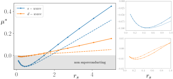
Figure 4: Plasmon-induced coupling constant $\mu^{*}$ as function of the electron gas density $r_{s}$ for $s$-and $d$-wave pairing channels. Solid line corresponds to an infinite inter-layer distance $a\rightarrow\infty$, dashed corresponds to $aq_{0}=1$. Right panel: detailed zoom on the electron density density range $r_{s}\in[0,1]$.

V Plasmon-assisted pairing

In this section we study how hyperbolic plasmons in a layered material affect other pairing mechanisms. We also provide an example of plasmon-engineering, where superconductivity is enhanced more efficiently.

V.1 Additional attractive interaction

We now consider the Migdal-Eliashberg equations in the presence of additional attractive interaction e.g. phonon- or magnon-induced. A physical origin of the additional attraction is not important for the model, we study, where on top of the Coulomb repulsion we add another pairing interaction in the $l$-wave angular momentum channel as follows [c.f., Eq. (22)]:

$${\cal V}_{k,k^{\prime}}^{(l)}(i\Omega_{n})\rightarrow{\cal V}_{k,k^{\prime}}^{(l)}(i\Omega_{n})-\lambda\frac{\omega_{0}^{2}}{\omega_{0}^{2}+\Omega_{n}^{2}}.$$

The numerical result of the solution of Eqs. (12) is shown in Fig. 1 (c) for the $d$-wave channel. Below we provide an explanation of the enhancement based on the toy model.

Analytically the transition temperature can be estimated using the same formalism as in Sec. IV.

$$T_{c}=1.134E_{F}e^{-1/\tilde{\mu}^{*}},$$ (28)

where $\tilde{\mu}^{*}=\lambda_{E_{F}}+\mu^{*}$, where $\mu^{*}$ is the coupling constant due to plasmons only and the from the other pairing mechanism gives rise to the effective coupling $\lambda_{E_{F}}\equiv\lambda/\left[1+\lambda\log\left(E_{F}/\omega_{0}\right)\right]$ renormalized to the Fermi energy scale. Provided that $\mu^{*}$ is approximately the same as we computed in the previous section we can expect the overall energy scale in Fig. 4 to be lifted by the amount of this renormalized coupling $\lambda_{E_{F}}$. This leads to the enhancement of the $d$-wave pairing.

We now solve the gap equation Eq. (23) including the additional attractive interaction Eq. (22). The result of full numerical solution is shown in Fig. 5 (a, b). We find an insignificant enhancement of superconductivity in the $s$-wave channel for $r_{s}<0.5$. In contrast, in the $d$-wave channel we find enhancement in a broad range of parameters as was expected from our toy model. As can be seen from Fig. 5 (c, d) the toy-model results are in good qualitative agreement with the Migdal-Eliasberg equation. In the following section we provide an example of modifying the hyperbolic metamaterial structure to achieve a plasmon dispersion that both enhances the superconductivity more efficiently in the $d$-wave channel and achieves a noticeable enhancement in the conventional $s$-wave channel.

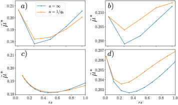
Figure 5: Superconducting coupling constant $\tilde{\mu}^{*}$ (eq. 28) extracted from solution of Migdal-Eliashberg equations. a) $s$-wave channel, b) $d$-wave channel. The toy-model results in the $s$- and $d$-wave channels are shown in (c, d). We take the following parameters for the additional coupling constant projected onto the corresponding angular momentum channel ${\cal V}=-\lambda\omega_{0}^{2}/(\omega_{0}^{2}+\Omega_{m}^{2}$): $\lambda=0.5,$ $\omega_{0}=E_{F}/10$.

V.2 Engineered plasmon-assisted enhancement

In this section, we show how the superconducting transition temperature can be enhanced by varying the electronic properties on one of the layers ($i=0$) as shown in Fig. 6 (a, b). Guided by the qualitative analysis of Sec. IV, we seek to reduce the screening energy range $\varepsilon_{\text{sc}}$ on the layer shown in red, which we label as $i=0$. This is expected to have a positive effect on the coupling strength based on the transition temperature estimate in Eqs. (27) and (28). As a simple proof-of-principle example, we show that this can occur if the target $i=0$ layer is distinct from the other layers. Experimentally this may correspond to inserting a layer of a different material with a higher standalone Fermi energy than that in the other layers (it may also occur by targeted gating/doping or naturally on a boundary layer). We do not specify a particular experimental realization, but point out that it seems to be a reasonable setup, as Fermi energies in different metals may vary by almost an order of magnitude (Ashcroft et al., 1976). For a quantitative description of the realistic metamaterial structures of this type, we may need to consider complications associated with a redistribution of charges, induced surface potentials in different layers due to tunneling, Volta barrier, etc. The form and shape of Fermi surfaces in different materials may also play a role.

We however disregard these possible complications and consider the simplified toy model instead, where both materials have a circular electronic dispersion, $\xi_{k}^{i}=k^{2}/2m_{i}-E_{F}^{(i)}$, with the the electron gas on the zeroth layer having a distinct Fermi energy $E_{F}^{(0)}$ and Fermi momentum $k_{F}^{(0)}$, while the other layers are characterized by $E_{F}^{(1)}$ and $k_{F}^{(1)}$ as shown in Fig. 6 (b). Denoting the bare Coulomb interaction matrix as ${\cal\widetilde{V}}_{{\bf q}}^{(i,j)}$, the complete RPA-renormalized interaction $\check{{\cal V}}_{{\bf q}}^{(i,j)}$ can be written in the following dimensionless matrix form (defined in the layer space parameterized by $i$ and $j$):

$$(\check{{\cal V}}_{{\bf q}}^{-1})^{(i,j)}=({\cal\widetilde{V}}_{{\bf q}}^{-1})^{(i,j)}+\delta_{i,j}q_{1}\Pi_{{\bf q}\zeta_{K}}\left(i\Omega_{n}\zeta_{E}\right)+\delta_{i,0}\delta_{j,0}\varXi_{{\bf q}},$$ (29)

where $\varXi_{{\bf q}}=q_{0}\Pi_{{\bf q}}\left(i\Omega_{n}\right)-q_{1}\Pi_{{\bf q}\zeta_{K}}\left(i\Omega_{n}\zeta_{E}\right)$, $\zeta_{E}=E_{F}^{\left(0\right)}/E_{F}^{\left(1\right)}$, $\zeta_{K}=k_{F}^{\left(0\right)}/k_{F}^{\left(1\right)}$ and $q_{0}$, $q_{1}$ are the Thomas-Fermi vectors of the $i=0$ and the rest layers respectively. The first two terms to the righthand side of Eq. (29) represent the inverse of the Coulomb interaction matrix in an infinite system of identical layers henceforth denoted as $({\cal V}_{{\bf q}}^{-1})^{(i,j)}\equiv({\cal\widetilde{V}}_{{\bf q}}^{-1})^{(i,j)}+\delta_{i,j}q^{(1)}\Pi_{{\bf q}\zeta_{K}}\left(i\Omega_{n}\zeta_{E}\right)$. The matrix inversion in Eq. (29) can be performed using the Sherman-Morrison formula (Sherman and Morrison, 1950):

$$\check{{\cal V}}_{{\bf q}}^{(i,j)} ={\cal V}_{{\bf q}}^{(i,j)}-\varXi_{{\bf q}}\frac{{\cal V}_{{\bf q}}^{\left(i,0\right)}{\cal V}_{{\bf q}}^{\left(0,j\right)}}{1+{\cal V}_{{\bf q}}^{\left(0,0\right)}\varXi_{{\bf q}}},$$ (30)

We thus expressed the interaction Eq. (29) in terms of the Coulomb propagator of a translationally-invariant system. The latter can be straightforwardly found in Fourier space. In particular, for the interaction on $i=0$ layer we get:

$$\check{{\cal V}}_{{\bf q}}^{\left(0,0\right)} =\frac{{\cal V}_{{\bf q}}^{\left(0,0\right)}}{1+{\cal V}_{{\bf q}}^{\left(0,0\right)}\varXi_{{\bf q}}}.$$ (31)

We now calculate the coupling constant induced by this interaction. We employ the following parametrization $\zeta_{K}=\sqrt{\zeta_{E}m_{1}/m_{0}}$ and vary only the $\zeta_{E}$ parameter for different electron mass ratios. Larger values $\zeta_{E}$ correspond to the lower value of the Fermi and screening energies $\varepsilon_{\text{sc}}$ of $i\neq 0$ layers. Based on the qualitative analysis in Sec. IV we thus expect to increase the coupling strength on $i=0$ layer. Numerically obtained coupling constant $\tilde{\mu}^{*}$ is shown in Fig. 6 (c, d) for pairing in $s$- and $d$-wave channels respectively. In case of the $d$-wave channel the additional enhancement of the coupling constant is found for all values $\zeta_{E}>1$. In the $s$-wave channel at low values of $\zeta_{E}$ we find that the layering is decreasing $\tilde{\mu}^{*}$. We also find that higher values of $\zeta_{E}$ tend to increase the coupling strength in accord with the qualitative discussion above. As a result we find that there is a threshold value of $\zeta_{E}$ above which the engineered layered structure enhances the electron pairing. In particular, for the electron mass ratio $m_{1}/m_{0}=3$ the threshold is $\zeta_{E}\approx 3$. At smaller electron mass rations the enhancement is expected to occur at larger values of $\zeta_{E}$.

In conclusion, in this section we studied the plasmon-assisted pairing in layered metals. We found a significant enhancement in the $d$-wave channel in the case of a perfectly regular metallic array. We also provided a way to engineer the plasmon environment in a layered metal such as to enhance Cooper pairing of electrons in both $s$- and $d$-wave channels.

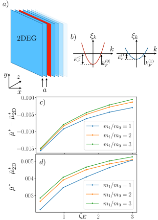
Figure 6: Engineered enhancement of superconductivity in a layered electron gas. a) Setup of an infinitely large layered electron gas with inter-layer distance $a$ the layer having distinct properties is shown in red. b) Electron properties on different layers: we assume massive dispersions but with the same Fermi momentum. Coupling constant $\tilde{\mu}^{*}$ in (c) $s$-wave and (d) $d$-wave (orange) channels as function of $\zeta_{E}$ for different electron mass ratios. The inter-layer distance and Wigner-Seitz parameters are respectively chosen to be $a=1/q_{0}$, $r_{s}=1$. The additional pairing parameters are $\lambda=1$, $\omega_{0}=0.1E_{F}$

VI Conclusions

The interplay between Coulomb interactions and superconductivity has been studied since the early days of superconductivity research. This includes numerous studies of the effect of plasmons on phonon-mediated superconductivity and also scenarios of plasmon-mediated superconductivity. It is therefore somewhat surprising that a standard Migdal-Eliashberg treatment of plasmons in layered materials, of obvious interest to the cuprates for example, has not been performed until this work. Here, we systematically studied various effects of plasmons in layered structures on superconductivity using both full Migdal-Eliashberg theory and qualitative arguments, which allowed us to develop useful intuition.

While we find neither an enhancement of $s$-wave pairing nor a plasmon-only pairing in hyperbolic structures, we do find a surprising effect of a sizable enhancement of $d$-wave pairing there. What it implies is that given a $d$-wave intrinsic superconductor (e.g., thin superconducting film), layering such films would lead to a significant enhancement of $T_{c}$. Furthermore, we point out that the “simple” layering is not the only possible way to affect the plasmon physics, and show that realistic paths exist to bootstrap both conventional $s$-wave and unconventional superconductivity to higher temperatures by engineering more favorable plasmon dispersions.

Apart from a possible connection to the layered oxide superconductors, there are additional arguments for why such a study is of interest and timely. Namely, there has been much interest (Curtis et al., 2019; Allocca et al., 2019; Schlawin et al., 2019; Sentef et al., 2018; Thomas et al., 2019; Kennes et al., 2021; Chen et al., 2020; Song and Gabor, 2018) recently in engineering electromagnetic environment (Rösner et al., 2018; Fatemi and Ruhman, 2018) in metamaterials and using cavities to achieve an enhancement of superconductivity. Of particular note are a series of works by Smolyaninova et al. (Smolyaninova et al., 2016, 2014), where a clear and significant enhancement of both transition temperature and critical field has been observed in fabricated aluminum/aluminum oxide layered structures. It was speculated that this could happen because of the anomalous hyperbolic plasmon dispersion, which may mediate superconductivity. The present work seems to rule out this scenario. This negative result however points towards phonons as a “culprit.” In particular, related hyperbolic phononic modes are of interest and will be discussed in a separate study.

Acknowledgements

The authors are grateful to Igor Smolyaninov and Sankar Das Sarma for helpful discussions. This work was supported by the National Science Foundation under Grant No. DMR-2037158, the U.S. Army Research Office under Contract No. W911NF1310172, and the Simons Foundation.

Appendix A Analytical solution

In this section we provide an exact solution of the gap equation in the case of a simplistic model, where the energy-dependence of the interaction is separable and is a product of two step-functions – a “square-well” model.

A.0.1 “Square-well” model

In order to get an analytical estimate of the superconducting transition temperature we assume the following separable form of the interaction in Eq. (25): $v_{m,n}\approx v_{n}v_{m}$ with $v_{n}=\theta(\varepsilon_{\text{sc}}^{2}-\varepsilon_{n}^{2})$. The gap equation becomes

$$\phi^{\left(i,j\right)}\left(i\varepsilon_{n}\right)=-\frac{\mu}{\beta}\sum_{m}\left(1-\sigma v_{n}v_{m}\right)f_{m}\phi^{(l)}\left(i\varepsilon_{m}\right),$$ (32)

where we denoted $f_{m}=\int_{-E_{F}}^{E_{F}}d\xi_{k^{\prime}}/(\varepsilon_{m}^{2}+\xi_{k^{\prime}}^{2})$. We note that since we work with dimensionless units, the Fermi energy is $E_{F}=1/4$. Due to the separability of the interaction, we define $A=\sum_{n}v_{n}f_{n}\phi^{\left(i,j\right)}\left(i\varepsilon_{n}\right)$ and $B=\sum_{n}\left(1-v_{n}\right)f_{n}\phi^{\left(i,j\right)}\left(i\varepsilon_{n}\right)$, which form the closed set of equations:

$$A= -\frac{\mu}{\beta}\left(A+B\right)\left(\sum f_{n}v_{n}\right)+\left(\sum f_{n}v_{n}\right)\frac{\mu\sigma}{\beta}A,$$

$$B= -\frac{\mu}{\beta}\left(A+B\right)\sum_{n}\left(1-v_{n}\right)f_{n}.$$

These equations lead to the self-consistency equation, which determines temperature condition.

$$1= \frac{\mu}{\beta}\left(\sigma-\frac{1}{1+\frac{\mu}{\beta}\sum_{n}\left(1-v_{n}\right)f_{n}}\right)\sum f_{n}v_{n}$$

We now use the following relations:

$$T \!\!\!\!\!\!\sum_{n}f_{n}v_{n} \approx\log\frac{2e^{\gamma}\varepsilon_{\text{sc}}\beta}{\pi},$$

$$T \!\!\!\!\!\!\!\!\!\sum_{n}f_{n} =\int_{0}^{E_{F}}d\xi_{k}\frac{\tanh\frac{\beta\xi_{k}}{2}}{\xi_{k}}\approx\log\frac{2e^{\gamma}E_{F}\beta}{\pi}.$$

By substituting this form to the Migdal-Eliashberg equation Eq. (32) and using (25) we readily find the transition temperature assuming $\varepsilon_{\text{sc}}\ll E_{F}$:

$$T_{c}=1.134\varepsilon_{\text{sc}}e^{-1/\mu_{\text{pl}}^{*}},$$ (33)

where

$$\mu_{\text{pl}}^{*}=\mu\left(\sigma-\frac{1}{1+\mu\log\frac{E_{F}}{\varepsilon_{\text{sc}}}}\right).$$ (34)

Superconductivity is only present if $\mu^{*}>0$. We observe that the Coulomb repulsion is strongly suppressed at the energy scales of order $\varepsilon_{\text{sc}}\ll E_{F}$ (Polchinski, 1992). Although the realistic interaction potential (see main text) is more complex than the one used in this Appendix, the qualitative arguments behind the result here – Eqs. (33) and (34) – are universal. Specifically, the transition temperature is primarily determined by two dimensionless parameters: $\sigma$ (effective screening strength) and $\varepsilon_{\text{sc}}/E_{F}$ (effective screening energy range).

Appendix B Pseudopotential method

In this section we provide details on the pseudopotential method, which we use to determine the effective pairing strength. The derivation follows Ref. (Grabowski and Sham, 1984). We start with the gap equation Eq (26):

$$\phi^{(l)}\left(i\varepsilon_{n}\right)=-T\sum_{m}{\cal V}\left(i\varepsilon_{n}-i\varepsilon_{m}\right)f_{m}\phi^{(l)}\left(i\varepsilon_{m}\right),$$

where $f_{m}=\int_{-E_{F}}^{E_{F}}d\xi_{k^{\prime}}\frac{1}{\varepsilon_{m}^{2}+\xi_{k^{\prime}}^{2}}$. We now introduce a low-energy frequency cut-off function $v_{n}=\theta\left(\varepsilon_{\text{c}}^{2}-\varepsilon_{n}^{2}\right)$ with the assumption $\varepsilon_{\text{c}}\ll\varepsilon_{\text{sc}}\ll E_{F}$.

$$\phi^{(l)}\left(i\varepsilon_{n}\right)= -T\sum_{m}{\cal V}\left(i\varepsilon_{n}-i\varepsilon_{m}\right)f_{m}v_{m}\phi^{(l)}\left(i\varepsilon_{m}\right)$$

$$-T\sum_{m}{\cal V}\left(i\varepsilon_{n}-i\varepsilon_{m}\right)f_{m}\left(1-v_{m}\right)\phi^{(l)}\left(i\varepsilon_{m}\right).$$

With this, we now integrate out the high-energy modes and find,

$$\phi^{(l)}\left(i\varepsilon_{n}\right)=-T\sum_{m}{\cal V}_{n,m}^{\text{eff}}f_{m}v_{m}\phi^{(l)}\left(i\varepsilon_{m}\right)$$ (35)

with ${\cal V}^{\text{eff}}$ obeying the equation,

$${\cal V}_{n,m}^{\text{eff}}=$$ (36)

$${\cal V}\left(i\varepsilon_{n}-i\varepsilon_{m}\right)-T\sum_{n^{\prime}}{\cal V}\left(i\varepsilon_{n}-i\varepsilon_{n^{\prime}}\right)\left(1-v_{n^{\prime}}\right){\cal V}_{n^{\prime},m}^{\text{eff}}.$$

If the cut-off energy is low enough, we can safely assume $\phi_{n}^{(l)}\approx\phi^{(l)}\left(i\varepsilon_{n=0}\right)$ and ${\cal V}_{n,m}^{\text{eff}}\approx{\cal V}_{0,0}^{\text{eff}}$. The critical temperature is then

$$T\approx\frac{2e^{\gamma}\varepsilon_{\text{co}}}{\pi}e^{\frac{1}{V_{0,0}^{\text{eff}}}}\approx 1.134\varepsilon_{\text{co}}e^{\frac{1}{V_{0,0}^{\text{eff}}}}$$

We thus identify the term $(-V_{0,0}^{\text{eff}})$ as the Coulomb pseudopotential at energy $\varepsilon_{\text{c}}$. In this approach, the problem of finding the critical temperature reduces to solving Eq. (36). The latter represents a system of linear equations, which can be solved numerically. An estimate can be obtained for the separable potential in analogy with the previous Appendix A.

Appendix C Kirzhnits-Maksimov-Khomskii theory

Here we briefly discuss the commonly-used approach by Kirzhnits, Maksimov, and Khomski (KMK) to plasmon-induced superconductivity based on Ref. (Kirzhnits et al., 1973). This theory deals with the gap equation in the real frequency domain as opposed to the Matsubara formalism in the conventional Eliashberg formulation presented in the main text. The gap equation in the KMK approach is of the BCS form:

$$\Delta_{p}=-\int d\xi_{k}K_{p,k}\frac{\tanh\frac{\beta\xi_{k}}{2}}{2\xi_{k}}\Delta_{k},$$ (37)

where the gap is defined as $\Delta_{p}\equiv 2\epsilon_{p}\int_{0}^{\infty}dxf\left(x,p\right)$ and $f$ is the analytical continuation of the pair propagator $F_{{\bf q},n}=-\int e^{i\varepsilon_{n}\tau}\langle\hat{\psi}_{{\bf q}}^{\left(i\right)}\left(\tau\right)\hat{\psi}_{-{\bf q}}^{\left(i\right)}\left(0\right)\rangle$. The kernel of the KMK gap equation (37) is given by

$$K_{p,k}=V_{p,k}^{\left(0\right)}-2\int_{0}^{\infty}d\varepsilon\frac{\text{Im}V_{p,k}^{R}\left(\varepsilon\right)}{\varepsilon+\left|\epsilon_{p}\right|+\left|\xi_{k}\right|},$$ (38)

where $V_{p,k}^{R}$ is the analytically continued interaction Eq. (4). KMK have derived Eq. (37) by performing the analytical continuation in the Eliashberg gap equation (23) and neglecting several terms that are not singular at the transition point. However, these terms are still be important for correct determination of the transition temperature, as was argued in Refs. (Schuh and Sham, 1983; Khan and Allen, 1980). The transition temperature in Eq. (37) can be estimated analytically assuming the separability of the interaction kernel $K$ analogously to Sec. A. We solve Eq. (37) numerically Takada (1978). The typical pairing strength is shown in Fig. 7. We find that the KMK approximation severely underestimates the pairing strength compared to the Migdal-Eliashberg equations. We therefore conclude that the KMK approach is quantitatively unreliable.

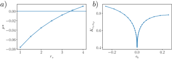
Figure 7: a) Coulomb pseudopotential for $a\rightarrow\infty$. b) effective interaction $K$ expressed in energy Eq. (38) for $r_{s}=2.5$.

Appendix D Effects of disorder in layer positions

In this section we study the effect of disorder in layer positions on the superconducting transition. For that we take the bare Coulomb interaction matrix as $\widetilde{{\cal V}}_{{\bf q}}^{(i,j)}=e^{-a_{i,j}q\left|i-j\right|}/q$, where $a_{i,j}$ is the set of random interlayer spacings. In the following we will treat $\widetilde{{\cal V}}_{{\bf q}}^{(i,j)}$ as a matrix in the layer-index space as in Sec. V.2. For the inter-layer spacings we assume $a_{i,j}=a_{i,j}^{(0)}+a_{i,j}^{\delta},$ where $a_{i,j}^{\delta}$ is a uniformly distributed random variable $a_{i,j}^{\delta}\in[0,\delta]$ and $a_{i,j}^{(0)}$ is the minimal inter-layer distance. Adopting the formalism of Sec. V.2, we write the interaction matrix in the absence of translational symmetry along $z$ axis as

$$({\cal V}_{{\bf q}}^{-1})^{(i,j)}=\left({\cal\widetilde{V}}_{{\bf q}}^{-1}\right)^{(i,j)}+\delta_{i,j}q_{0}\Pi_{{\bf q}}\left(i\Omega_{n}\right).$$ (39)

Below we find the transition temperature corresponding to Eliashberg equations with interaction (39).

D.0.1 Plasmon localization

Plasmon modes in a disordered layered gas correspond to the eigenvalues of the matrix (39). We denote them as $\left\{\lambda\right\}$ and the corresponding eigenvectors as $\{\zeta_{j}^{\left(\lambda\right)}\}$:

$$\sum_{j}{\cal V}_{{\bf q}}^{(i,j)}(i\Omega_{n})\zeta_{j}^{(\lambda)}=\epsilon_{\lambda}\zeta_{i}^{(\lambda)}.$$ (40)

Here, the eigenvalues are functions of both the in-plane momentum ${\bf q}$ and the frequency $i\Omega_{n}$: $\epsilon_{\lambda}=\epsilon_{\lambda}\left(i\Omega_{n}\right)$. The typical eigenvector of Eq. (40) is shown in Fig. 8 (a), where performed the analytic continuation to real frequencies $i\Omega_{n}\rightarrow\omega+i0^{+}$. We observe Anderson localisation Sarma et al. (1986) of plasmons in the apical direction (Anderson, 1958) for $N=50$ layers. In Fig. 8 (b) we study the effective interaction between layers close to the center of the sample. More precisely, we consider the approach of Sec. (IV) for the disorder interaction given in Eq. (39). As can be seen in Fig. 8 (b) the interaction is barely affected by the disorder. We therefore conclude that disorder does not modify the critical temperature.

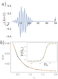
Figure 8: Anderson localization of plasmons. a) Typical plasmon distribution for the lowest eigenvalue $\lambda=1$ (Eq. 40), b) Typical static interaction ${\cal V}\left(0\right)$ as function of the electron gas Wigner-Seitz density parameter $r_{s}$ for 8 layers: the random layer spacing $a_{i,j}=a_{i,j}^{(0)}+a_{i,j}^{\delta}$ shown in blue with the average spacing $a_{i,j}^{\left(0\right)}=q_{0}^{-1}$ and $\delta=q_{0}^{-1}$, regular array result shown in orange. Inset shows the interaction as function of the imaginary frequency $\Omega_{n}$. The infinite layer number is shown in green color for comparison.

Appendix E Finite thickness of layers

In this section we consider the setup with the finite-thickness layers Bondarev et al. (2020); Bondarev and Shalaev (2017). In this section we follow the approach Sarma (1984). For a given thickness $w$ of each layer we now need to keep the quantization of electron wavefuntion along the $z$ direction. The generalization of electron polarization operator can be written as:

$$\Pi_{{\bf q}}^{\left(w\right)}\left(i\Omega_{m},z,z^{\prime}\right) =\frac{T}{A}\sum_{{\bf k},n}\sum_{l,l^{\prime}}\frac{\zeta_{l}\left(z\right)\zeta_{l}\left(z^{\prime}\right)}{i\varepsilon_{n}-\epsilon_{{\bf k}}-\frac{k_{l}^{2}}{2m}}$$

$$\times\frac{\zeta_{l^{\prime}}\left(z\right)\zeta_{l^{\prime}}\left(z^{\prime}\right)}{i\varepsilon_{n}+i\Omega_{m}-\epsilon_{{\bf k}+{\bf q}}-\frac{k_{l^{\prime}}^{2}}{2m}},$$

where $\zeta_{l}\left(z\right)\equiv\sqrt{2/w}\sin(k_{l}z)$ denotes the $l$-th subband mode profile of the electron gas and $k_{l}=\pi l/w$ with $l\in\mathbb{Z}$. Here we restrict to the case when layers are sufficiently thin and restrict our consideration to the lowest-energy sub-band:

$$\Pi_{q}^{\left(w\right)}\left(z,z^{\prime}\right)\approx\zeta_{1}^{2}\left(z\right)\zeta_{1}^{2}\left(z^{\prime}\right)\Pi_{q},$$ (41)

where $\Pi_{q}$ is the usual two-dimensional polarization operator. It is now convenient to project the Coulomb interaction onto the lowest sub-band wavefunction. In particular, for the bare interaction we have:

$${\cal\widetilde{V}}_{{\bf q}}^{\left(i,j\right)}\left(w\right) \equiv\frac{1}{q}\int dzdz^{\prime}e^{-q\left|z-z^{\prime}\right|}\zeta_{1}^{2}\left(z+ai\right)\zeta_{1}^{2}\left(z^{\prime}+aj\right).$$

This integral can be taken analytically. In particular for $i\neq j$ we find:

$${\cal\widetilde{V}}_{{\bf q}}^{\left(i\neq j\right)}\left(w\right)=\widetilde{{\cal V}}_{{\bf q}}^{\left(i\neq j\right)}\left(w=0\right)\times\frac{16\pi^{4}e^{-wq}\left(e^{wq}-1\right)^{2}}{w^{2}q^{2}\left(w^{2}q^{2}+4\pi^{2}\right)^{2}}.$$ (42)

The term $i=j$ is more cumbersome and we will not reproduce it here. We now transform into Fourier space with respect to the layer index and get:

$$\widetilde{{\cal V}}_{{\bf q},q_{z}}\left(w\right) =\sum_{j\neq 0}e^{-iq_{z}j}\widetilde{{\cal V}}_{{\bf q}}^{\left(j,0\right)}\left(w\right)+\widetilde{{\cal V}}_{{\bf q}}^{\left(0,0\right)}\left(w\right)$$

$$=\frac{1}{q}\frac{\sinh aq}{\cosh aq-\cos q_{z}}\frac{16\pi^{4}e^{-wq}\left(e^{wq}-1\right)^{2}}{w^{2}q^{2}\left(w^{2}q^{2}+4\pi^{2}\right)^{2}}$$

$$+\widetilde{{\cal V}}_{{\bf q}}^{\left(0,0\right)}\left(w\right)-\frac{1}{q}\times\frac{16\pi^{4}e^{-wq}\left(e^{wq}-1\right)^{2}}{w^{2}q^{2}\left(w^{2}q^{2}+4\pi^{2}\right)^{2}}$$

We this we can now repeat the same procedure of RPA renormalization of interaction.

$${\cal V}_{{\bf q},q_{z}}\left(i\Omega_{m},w\right)=\frac{1}{\widetilde{{\cal V}}_{{\bf q},q_{z}}^{-1}(w)+q_{0}\Pi_{{\bf q}}\left(i\Omega_{m}\right)}.$$

As shown in Fig. 9 the effect of layer thickness on the transition temperature is insignificant under our approximations.

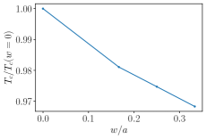
Figure 9: Superconducting transition temperature as function of layer thickness. Simulation parameters are chosen as $a=1/q_{0}$, $r_{s}=1$, $\lambda=1$.

References

- Basov et al. (2021) D. Basov, A. Asenjo-Garcia, P. J. Schuck, X. Zhu, and A. Rubio, Nanophotonics 10, 549 (2021).
- Shekhar et al. (2014) P. Shekhar, J. Atkinson, and Z. Jacob, Nano Convergence 1, 14 (2014).
- Hawrylak et al. (1988) P. Hawrylak, G. Eliasson, and J. J. Quinn, Phys. Rev. B 37, 10187 (1988).
- Poddubny et al. (2013) A. Poddubny, I. Iorsh, P. Belov, and Y. Kivshar, Nature photonics 7, 948 (2013).
- Smolyaninov (2018) I. I. Smolyaninov, in World Scientific Handbook of Metamaterials and Plasmonics: Volume 1: Electromagnetic Metamaterials (World Scientific, 2018) pp. 87–138.
- Cortes and Jacob (2017) C. L. Cortes and Z. Jacob, Nature communications 8, 1 (2017).
- Das Sarma and Quinn (1982) S. Das Sarma and J. J. Quinn, Phys. Rev. B 25, 7603 (1982).
- Jain and Das Sarma (1987) J. K. Jain and S. Das Sarma, Phys. Rev. B 36, 5949 (1987).
- Morawitz et al. (1993) H. Morawitz, I. Bozovic, V. Kresin, G. Rietveld, and D. Van Der Marel, Zeitschrift für Physik B Condensed Matter 90, 277 (1993).
- Kresin and Morawitz (1988) V. Z. Kresin and H. Morawitz, Phys. Rev. B 37, 7854 (1988).
- Bill et al. (2003) A. Bill, H. Morawitz, and V. Kresin, Physical Review B 68, 144519 (2003).
- Takada (1978) Y. Takada, Journal of the Physical Society of Japan 45, 786 (1978).
- Takada (1992) Y. Takada, Journal of the Physical Society of Japan 61, 238 (1992).
- Kirzhnits et al. (1973) D. A. Kirzhnits, E. G. Maksimov, and D. I. Khomskii, Journal of Low Temperature Physics 10, 79 (1973).
- Schuh and Sham (1983) B. Schuh and L. J. Sham, Journal of Low Temperature Physics 50, 391 (1983).
- Khan and Allen (1980) F. Khan and P. Allen, Solid State Communications 36, 481 (1980).
- Rietschel and Sham (1983) H. Rietschel and L. J. Sham, Phys. Rev. B 28, 5100 (1983).
- Grabowski and Sham (1984) M. Grabowski and L. J. Sham, Phys. Rev. B 29, 6132 (1984).
- Smolyaninova et al. (2016) V. N. Smolyaninova, C. Jensen, W. Zimmerman, J. C. Prestigiacomo, M. S. Osofsky, H. Kim, N. Bassim, Z. Xing, M. M. Qazilbash, and I. I. Smolyaninov, Scientific Reports 6, 34140 (2016).
- Smolyaninova et al. (2014) V. N. Smolyaninova, B. Yost, K. Zander, M. S. Osofsky, H. Kim, S. Saha, R. L. Greene, and I. I. Smolyaninov, Scientific Reports 4, 7321 (2014).
- Liberal and Engheta (2017) I. Liberal and N. Engheta, Nature Photonics 11, 149 (2017).
- Marsiglio (2020) F. Marsiglio, Annals of Physics 417, 168102 (2020).
- Tsuei and Kirtley (2000) C. Tsuei and J. Kirtley, Physical review letters 85, 182 (2000).
- Little (1964) W. A. Little, Phys. Rev. 134, A1416 (1964).
- Ashcroft et al. (1976) N. W. Ashcroft, N. D. Mermin, et al., “Solid state physics,” (1976).
- Sherman and Morrison (1950) J. Sherman and W. J. Morrison, The Annals of Mathematical Statistics 21, 124 (1950).
- Curtis et al. (2019) J. B. Curtis, Z. M. Raines, A. A. Allocca, M. Hafezi, and V. M. Galitski, Phys. Rev. Lett. 122, 167002 (2019).
- Allocca et al. (2019) A. A. Allocca, Z. M. Raines, J. B. Curtis, and V. M. Galitski, Phys. Rev. B 99, 020504 (2019).
- Schlawin et al. (2019) F. Schlawin, A. Cavalleri, and D. Jaksch, Phys. Rev. Lett. 122, 133602 (2019).
- Sentef et al. (2018) M. A. Sentef, M. Ruggenthaler, and A. Rubio, Science Advances 4, eaau6969 (2018), https://www.science.org/doi/pdf/10.1126/sciadv.aau6969 .
- Thomas et al. (2019) A. Thomas, E. Devaux, K. Nagarajan, T. Chervy, M. Seidel, D. Hagenmüller, S. Schütz, J. Schachenmayer, C. Genet, G. Pupillo, et al., arXiv preprint arXiv:1911.01459 (2019).
- Kennes et al. (2021) D. M. Kennes, M. Claassen, L. Xian, A. Georges, A. J. Millis, J. Hone, C. R. Dean, D. N. Basov, A. N. Pasupathy, and A. Rubio, Nature Physics 17, 155 (2021).
- Chen et al. (2020) X. Chen, X. Fan, L. Li, N. Zhang, Z. Niu, T. Guo, S. Xu, H. Xu, D. Wang, H. Zhang, A. S. McLeod, Z. Luo, Q. Lu, A. J. Millis, D. N. Basov, M. Liu, and C. Zeng, Nature Physics 16, 631 (2020).
- Song and Gabor (2018) J. C. W. Song and N. M. Gabor, Nature Nanotechnology 13, 986 (2018).
- Rösner et al. (2018) M. Rösner, R. Groenewald, G. Schoenhoff, J. Berges, S. Haas, and T. O. Wehling, arXiv preprint arXiv:1803.04576 (2018).
- Fatemi and Ruhman (2018) V. Fatemi and J. Ruhman, Phys. Rev. B 98, 094517 (2018).
- Polchinski (1992) J. Polchinski, arXiv preprint hep-th/9210046 (1992).
- Sarma et al. (1986) S. D. Sarma, A. Kobayashi, and R. Prange, Physical review letters 56, 1280 (1986).
- Anderson (1958) P. W. Anderson, Phys. Rev. 109, 1492 (1958).
- Bondarev et al. (2020) I. V. Bondarev, H. Mousavi, and V. M. Shalaev, Physical review research 2, 013070 (2020).
- Bondarev and Shalaev (2017) I. V. Bondarev and V. M. Shalaev, Optical Materials Express 7, 3731 (2017).
- Sarma (1984) S. D. Sarma, Physical Review B 29, 2334 (1984).