Investigating the architecture and internal structure of the TOI-561 system planets with CHEOPS, HARPS-N and TESS

Abstract

We present a precise characterization of the TOI-561 planetary system obtained by combining previously published data with TESS and CHEOPS photometry, and a new set of $62$ HARPS-N radial velocities (RVs). Our joint analysis confirms the presence of four transiting planets, namely TOI-561 b ($P=0.45$ d, $R=1.42$ R_⊕, $M=2.0$ M_⊕), c ($P=10.78$ d, $R=2.91$ R_⊕, $M=5.4$ M_⊕), d ($P=25.7$ d, $R=2.82$ R_⊕, $M=13.2$ M_⊕) and e ($P=77$ d, $R=2.55$ R_⊕, $M=12.6$ R_⊕). Moreover, we identify an additional, long-period signal ($>450$ d) in the RVs, which could be due to either an external planetary companion or to stellar magnetic activity. The precise masses and radii obtained for the four planets allowed us to conduct interior structure and atmospheric escape modelling. TOI-561 b is confirmed to be the lowest density ($\rho_{\rm b}=3.8\pm 0.5$ g cm^-3) ultra-short period (USP) planet known to date, and the low metallicity of the host star makes it consistent with the general bulk density-stellar metallicity trend. According to our interior structure modelling, planet b has basically no gas envelope, and it could host a certain amount of water. In contrast, TOI-561 c, d, and e likely retained an H/He envelope, in addition to a possibly large water layer. The inferred planetary compositions suggest different atmospheric evolutionary paths, with planets b and c having experienced significant gas loss, and planets d and e showing an atmospheric content consistent with the original one. The uniqueness of the USP planet, the presence of the long-period planet TOI-561 e, and the complex architecture make this system an appealing target for follow-up studies.

1 Introduction

Since the announcement of the first exoplanet orbiting a Sun-like star (Mayor & Queloz, 1995), the growing number of discoveries in exoplanetary science have yielded a surprising variety of exoplanets and exoplanetary systems. The field has benefited hugely from dedicated space-based missions, such as CoRoT, Kepler, K2 (Baglin et al., 2006; Borucki et al., 2010; Howell et al., 2014), and recently TESS (Ricker et al., 2014). With more than $170$ confirmed planets, and $\sim 4000$ planet candidates, the majority of which will likely turn out to be planets, TESS has increased the census of confirmed exoplanets to more than $4500$. Alongside the aforementioned missions, which are designed to discover a large number of exoplanets by searching for transit-like signatures around hundreds of thousands of stars, new characterization missions, with a specific focus on the detailed study of known exoplanets, are now starting to operate. Among them, the CHaracterising ExOPlanet Satellite (CHEOPS, Benz et al. 2021), launched on 18 December 2019, is a $30$ cm telescope which is collecting ultra-high precision photometry of known exoplanets, aiming at their precise characterization. CHEOPS met its precision requirements both on bright and faint stars, achieving a noise level of $\sim 15$ ppm per $6$ h intervals for $V\sim 9$ mag stars, and $75$ ppm per $3$ h for $V\sim 12$ mag stars (Benz et al., 2021). The importance of such a high photometric precision is reflected in CHEOPS’ first scientific results, which span a variety of different fields (Lendl et al. 2020; Bonfanti et al. 2021b; Leleu et al. 2021; Delrez et al. 2021; Morris et al. 2021a; Borsato et al. 2021; Van Grootel et al. 2021; Szabó et al. 2021; Hooton et al. 2021; Swayne et al. 2021; Maxted et al. 2021; Barros et al. 2022; Wilson et al. 2022; Deline et al. 2022). As part of its main scientific goals, CHEOPS is refining the radii of known exoplanets to achieve the precision on the bulk density needed for internal structure and atmospheric evolution modelling. To fulfil this aim, radial velocity (RV) follow-ups using high-precision spectrographs are essential to provide the precise planetary masses that can be combined with radii measurements to determine accurate densities. Among the exoplanets having both radius and mass measurements, the ones in well-characterised multiplanetary systems are of particular interest, since they allow for investigation of their formation and evolution processes through comparative planetology, e.g. by comparing their individual inner bulk compositions (e.g. Guenther et al. 2017; Prieto-Arranz et al. 2018), by studying their mutual inclinations and eccentricities (e.g. Fabrycky et al. 2014; Van Eylen et al. 2019; Mills et al. 2019), and by investigating the correlations between their relative sizes, masses and orbital separations (e.g. Lissauer et al. 2011; Ciardi et al. 2013; Millholland et al. 2017; Weiss et al. 2018; Jiang et al. 2020; Adams et al. 2020).

Within this context, TOI-561, announced simultaneously by Lacedelli et al. (2021) and Weiss et al. (2021) (L21 and W21 hereafter, respectively), is a particularly interesting system, both from the stellar (Section 2.1) and planetary (Section 2.2) perspective. The low stellar metallicity, the presence of an ultra-short period (USP) planet, where USP planets are meant here as planets with periods shorter than one day and radii smaller than $2$ R_⊕, and the complexity of its planetary configuration make TOI-561 an appealing target for in-depth investigations. In this study, we combine literature data with new TESS observations (Section 3.1), CHEOPS photometry (Section 3.2), and HARPS-N RVs (Section 3.3) to shed light on the planetary architecture and infer the internal structure of the transiting planets. After assessing the planetary configuration using CHEOPS observations (Section 4.1) and performing a thorough analysis of the global RV data set (Section 4.2), we jointly modelled the photometric and spectroscopic data to obtain the planetary parameters (Section 5). We used our derived stellar and planetary properties to model the internal structures of the transiting planets (Section 6) and their atmospheric evolution (Section 7), before discussing our results and presenting our conclusions (Section 8).

2 The TOI-561 system

2.1 The host star

TOI-561 is an old, metal-poor, thick disk star (L21, W21), slightly smaller and cooler than the Sun, located $\sim 84$ pc away from the Solar System. We report the main astrophysical properties of the star in Table 1.

We adopted the spectroscopic parameters and stellar abundances from L21 (Table 1), which were derived exploiting the high SNR, high-resolution HARPS-N co-added spectrum (L21, § 3.1) through an accurate analysis using three independent methods, namely the ARES+MOOG equivalent width method (Sousa, 2014; Mortier et al., 2014), the Stellar Parameter Classification (Buchhave et al., 2012, 2014) and the CCFpams method (Malavolta et al., 2017).

Taking advantage of the updated parameters coming from the Gaia EDR3 release (Gaia Collaboration et al., 2021), we then used the L21 spectral parameters as priors on spectral energy distribution selection to infer the stellar radius ($R_{\star}$) of TOI-561 using the infrared flux method (IRFM, Blackwell & Shallis 1977). The IRFM compares optical and infrared broadband fluxes and synthetic photometry of stellar atmospheric models, and uses known relationships between stellar angular diameter, $T_{{\rm eff}}$ and parallax to derive $R_{\star}$, in a MCMC fashion as detailed in Schanche et al. (2020). For this study, we retrieved from the most recent data releases the Gaia G, G_BP, G_RP (Gaia Collaboration et al., 2021), 2MASS $J$, $H$, $K$ (Skrutskie et al., 2006), and WISE $W1$, $W2$ (Wright et al., 2010) broadband photometric magnitudes, and we used the stellar atmospheric models from the ATLAS Catalogues (Castelli & Kurucz, 2003) and the Gaia EDR3 parallax with the offset of Lindegren et al. (2021) applied, to obtain $R_{\star}$ $=0.843\pm 0.005$ R_⊙.

We combined two different sets of stellar evolutionary tracks and isochrones, PARSEC (PAdova & TRieste Stellar Evolutionary Code, v1.2S; Marigo et al., 2017) and CLES (Code Liègeois d’Évolution Stellaire, Scuflaire et al., 2008), to derive the stellar mass ($M_{\star}$) and age ($t_{\star}$) of TOI-561. As the star is significantly alpha-enhanced, we avoided using $[$Fe/H$]$ as a proxy for the stellar metallicity; instead, we inserted both $[$Fe/H$]$ and [$\alpha$/Fe] in relation (3) provided by Yi et al. (2001), obtaining an overall scaling of metal abundances $\mathrm{[M/H]}=-0.23\pm 0.06$. Besides $[$M/H$]$, the main input parameters for computing $M_{\star}$ and $t_{\star}$ were $T_{\mathrm{eff}}$ and $R_{\star}$. In addition, we used as inputs $\log{\rm R}^{\prime}_{\rm HK}$ and the upper limit on $v$ sin $i$ from L21, and the yttrium over magnesium abundance $\mathrm{[Y/Mg]}=-0.22\pm 0.07$, as computed from $[$Mg/H$]$ and $[$Y/H$]$ reported by W21. These indices improve the model convergence by discarding unlikely young isochrones, as broadly discussed in Section 2.2.3 of Bonfanti & Gillon (2020), and references therein. The PARSEC results were obtained using the isochrone placement algorithm of Bonfanti et al. (2015, 2016), which retrieves the best-fit parameters by interpolating within a pre-computed grid of models, while the CLES algorithm models directly the star through a Levenberg-Marquardt minimisation (Salmon et al., 2021). The final adopted values ($M_{\star}=0.806\pm 0.036$ M_⊙, $t_{\star}=11.0_{-3.5}^{+2.8}$ Gyr) are a combination of the outputs from both sets of models, as described in detail in Bonfanti et al. (2021b). The derived mass and radius, listed in Table 1, are consistent within $1\sigma$ with the values reported in L21 ($\mbox{$R_{\star}$}=0.849\pm 0.007$ R_⊙, $\mbox{$M_{\star}$}=0.785\pm 0.018$ M_⊙).

Table 1: Stellar properties of TOI-561.

[t] TOI-561 TIC 377064495 Gaia EDR3 3850421005290172416 2MASS J09524454+0612589 Parameter Value Source RA (J2016; hh:mm:ss.ss) 09:52:44.43 A Dec (J2016; dd:mm:ss.ss) $+$06:12:57.94 A $\mu_{\alpha}$ (mas yr^-1) $-108.504\pm 0.022$ A $\mu_{\delta}$ (mas yr^-1) $-61.279\pm 0.019$ A $\gamma$ (km s^-1) $79.54\pm 0.56$ A Parallax (mas) $11.8342\pm 0.0208$ A Distance (pc) $84.25\pm 0.12$ B TESS (mag) $9.527\pm 0.006$ C G (mag) $10.0181\pm 0.0028$ A G_BP (mag) $10.3945\pm 0.0028$ A G_RP (mag) $9.4692\pm 0.0038$ A V (mag) $10.252\pm 0.006$ C B (mag) $10.965\pm 0.082$ C J (mag) $8.879\pm 0.020$ D H (mag) $8.504\pm 0.055$ D K (mag) $8.394\pm 0.019$ D W1 (mag) $8.337\pm 0.023$ E W2 (mag) $8.396\pm 0.020$ E $T_{{\rm eff}}$ (K) $5372\pm 70$ F log g  (cgs) $4.50\pm 0.12$ F $[{\rm Fe}/{\rm H}]$  (dex) $-0.40\pm 0.05$ F $[$Mg/H$]$ (dex) $-0.17\pm 0.05$ F $[$Si/H$]$ (dex) $-0.22\pm 0.05$ F $[$Ti/H$]$ (dex) $-0.12\pm 0.03$ F $[\alpha$/Fe$]$ (dex) $0.23\pm 0.04$ F $[$M/H$]$ (dex) $-0.23\pm 0.06$ G $[$Y/Mg$]$ (dex) $-0.22\pm 0.07$ G^a $\log{\rm R}^{\prime}_{\rm HK}$ $-5.003\pm 0.012$ F $v$ sin $i$ (km s^-1) $<2$ F $R_{\star}$ (R_⊙) $0.843\pm 0.005$ G, IRFM $M_{\star}$ (M_⊙) $0.806\pm 0.036$ G, isochrones $t_{\star}$ (Gyr) $11.0_{-3.5}^{+2.8}$ G, isochrones $\rho_{\star}$ ($\rho_{\odot}$) $1.34\pm 0.06$ G, from $R_{\star}$ and $M_{\star}$ $\rho_{\star}$ (g cm^-3) $1.89\pm 0.09$ G, from $R_{\star}$ and $M_{\star}$ $L_{\star}$ ($L_{\odot}$) $0.533\pm 0.029$ G, from $R_{\star}$ and $T_{{\rm eff}}$ Spectral type G9V F

• A) Gaia EDR3 (Gaia Collaboration et al., 2021). B) Bailer-Jones et al. (2021). C) TESS Input Catalogue Version 8 (TICv8, Stassun et al. 2018). D) Two Micron All Sky Survey (2MASS, Cutri et al. 2003). E) Wide-field Infrared Survey Explorer (WISE; Wright et al., 2010). F) L21. G) This work.
  ^a Based on W21 abundances.

2.2 The planetary system

The discovery of a multiplanetary system orbiting TOI-561 was announced simultaneously by L21 and W21 in two independent papers. The main planetary parameters from both studies are reported in Table 2.

The two papers presented different RV data sets, collected with HARPS-N and HIRES respectively, to confirm the planetary nature of three candidates identified by TESS in sector $8$, the only available sector at the time of the publications. The TESS-identified signals had periods of $\sim 0.45$, $\sim 10.8$, and $\sim 16$ days. The two inner candidates were confirmed by both L21 and W21, with the names of TOI-561 b (an USP super-Earth, with period $P_{\rm b}\sim 0.4465$ d, and radius $R_{\rm b}\sim 1.4$ R_⊕), and TOI-561 c (a warm mini-Neptune, with $P_{\rm c}\sim 10.779$ d, and $R_{\rm c}\sim 2.9$ R_⊕). However, two different interpretations for the third TESS signal were proposed by the authors. In the scenario presented in L21, the two transits related to the third TESS signal were interpreted as single transits of two distinct planets, TOI-561 d ($P_{\rm d}\sim 25.6$ d, $R_{\rm d}\sim 2.5$ R_⊕), and TOI-561 e ($P_{\rm e}\sim 77$ d, $R_{\rm e}\sim 2.7$ R_⊕). The periods of these two planets were inferred from the RV analysis, which played an essential role in determining the final planetary architecture. In fact, the ephemeris match between the RV and photometric fits (See Fig. 5 of L21) and the non-detection of the $16$ d signal in the HARPS-N data set, combined with the different durations of the two TESS transits and results from the long-term stability analysis led the authors to converge on a 4-planet configuration, presenting robust mass and radius detection for all the four planets in the system (L21, Table 5). In contrast, W21 proposed the presence of a single planet at the period suggested by TESS (TOI-561 f, $P_{\rm f}\sim 16.29$ d, $R_{\rm f}\sim 2.3$ R_⊕), based on the analysis of the two available transits. W21 pointed out that the $8.1$ d alias of planet f’s orbital period is also consistent with the TESS data, with the even transit falling into the TESS download gap, even though in this case the transit duration would be too long compared to what is expected for a 8 d period planet (§4.9, W21). However, the authors could not obtain an accurate mass determination for this planet, with the $60$ HIRES RVs being consistent with a non-detection (§ 7.2, W21). An additional discrepancy between the two studies is the mass of the USP planet, differing by almost a factor two. According to the W21 analysis, TOI-561 b has a mass of $3.2\pm 0.8$ M_⊕, making it consistent with a rocky composition and placing it among the population of typical small ($<2$ R_⊕), extremely irradiated USP planets (Sanchis-Ojeda et al., 2015; Dai et al., 2021). Instead, assuming the low mass ($M_{\rm b}=1.59\pm 0.36$ M_⊕) inferred from L21 analysis, TOI-561 b is not consistent with a pure rocky composition, and it is the lowest density USP super-Earth known to date, calling for a more complex interpretation (e.g. lighter core composition, deep water reservoirs, presence of a high-metallicity, volatile materials or water steam envelope, etc.).

The complexity of this system and the differences between the two studies demanded further investigations. We therefore decided to collect additional, precise photometric and RV data (Section 3) to shed light on the planetary configuration and on the internal composition of the TOI-561 planets.

Table 2: Literature parameters of the proposed planets orbiting TOI-561.

[t] TOI-561 b Lacedelli et al. (2021) Weiss et al. (2021) $P$ (d) $0.446578\pm 0.000017$ $0.446573^{+0.000032}_{-0.000021}$ $T_{0}$ (TBJD) $1517.498\pm 0.001$ $1517.4973\pm 0.0018$ $R_{\rm p}$ (R_⊕) $1.423\pm 0.066$ $1.45\pm 0.11$ $K$ (m s^-1) $1.56\pm 0.35$ $3.1\pm 0.8$ $M_{\rm p}$ (M_⊕) $1.59\pm 0.36$ $3.2\pm 0.8$ TOI-561 c $P$ (d) $10.779\pm 0.004$ $10.77892\pm 0.00015$ $T_{0}$ (TBJD) $1527.060\pm 0.004$ $1527.05825\pm 0.00053$ $R_{\rm p}$ (R_⊕) $2.878\pm 0.096$ $2.90\pm 0.13$ $K$ (m s^-1) $1.84\pm 0.33$ $2.4\pm 0.8$ $M_{\rm p}$ (M_⊕) $5.40\pm 0.98$ $7.0\pm 2.3$ TOI-561 d $P$ (d) $25.62\pm 0.04$ - $T_{0}$ (TBJD) $1521.882\pm 0.004$ - $R_{\rm p}$ (R_⊕) $2.53\pm 0.13$ - $K$ (m s^-1) $3.06\pm 0.33$ - $M_{\rm p}$ (M_⊕) $11.95\pm 1.28$ - TOI-561 e $P$ (d) $77.23\pm 0.39$ - $T_{0}$ (TBJD) $8538.181\pm 0.004$ - $R_{\rm p}$ (R_⊕) $2.67\pm 0.11$ - $K$ (m s^-1) $2.84\pm 0.41$ - $M_{\rm p}$ (M_⊕) $16.0\pm 2.3$ - TOI-561 f$\,{}^{a}$ $P$ (d) - $16.287\pm 0.005$ $T_{0}$ (TBJD) - $1521.8828\pm 0.0035$ $R_{\rm p}$ (R_⊕) - $2.32\pm 0.16$ $K$ (m s^-1) - $0.9\pm 0.6$ $M_{\rm p}$ (M_⊕) - $3.0^{+2.4}_{-1.9}$ $\mathrm{\mbox{$M_{\star}$}\ (\mbox{M${}_{\odot}$})}$ $0.785\pm 0.018$ $0.805\pm 0.030$

• ^a Referred as TOI-561 d in W21.

3 Observations

3.1 TESS photometry

During its two-year primary mission (Ricker et al., 2014), TESS observed TOI-561  in two-minute cadence mode between 2 February and 27 February 2019 (sector $8$). After entering its extended mission, TESS re-observed the star in two-minute cadence mode during sector $35$, between 9 February and 6 March 2021. At the beginning of the second orbit, the spacecraft dropped out of Fine Pointing mode for $3.44$ days, entering Coarse Pointing mode. Data collected during Coarse Pointing mode were flagged and removed from the Pre-search Data Conditioning Simple Aperture Photometry (PDCSAP, Smith et al., 2012; Stumpe et al., 2012; Stumpe et al., 2014) light curves, leading to a total of $19.86$ days of science data. The photometric observations of TOI-561 were reduced by the Science Processing Operations Center (SPOC) pipeline and searched for evidence of transiting planets (Jenkins et al., 2016; Jenkins, 2020). For our photometric analysis, we used the light curves based on the PDCSAP, downloading the two-minute cadence data from the Mikulski Archive for Space Telescopes (MAST), and removing all the observations encoded as NaN or flagged as bad-quality (DQUALITY>0) points by the SPOC pipeline. We performed outlier rejection by doing a cut at $3\sigma$ for positive outliers and $5\sigma$ (i. e. larger than the deepest transit) for negative outliers. The resulting TESS light curves of sectors 8 and 35 are shown in Figure 1, and Table 3 summarizes the total number of transits observed by TESS for each planet.

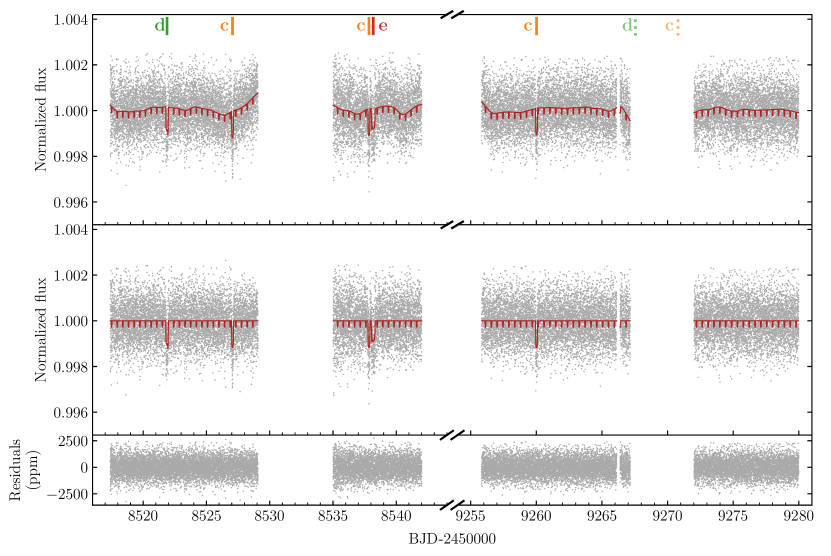
Figure 1: TESS sector $8$ (left) and $35$ (right) PDCSAP light curves of TOI-561. In the top panel, the dark red solid line shows the best-fitting transit and Matérn-3/2 kernel Gaussian Process (GP) model, as detailed in Section 5. The central panel shows the flattened light curve after the removal of the GP component, with the best-fitting transit model superimposed (dark red solid line). The transits of planets c, d and e are labelled and highlighted with orange, green and red vertical lines, respectively. The expected locations of the transits of planets c and d occurring during the data gaps of sector 35 are marked with pale, dashed orange and green lines, respectively. Planet e is not expected to transit in sector 35. The transits of the USP planet are too shallow to be individually visible, and are not indicated. Light curve residuals are shown in the bottom panel.

To refine the ephemeris of planet d in time for the scheduling of the CHEOPS observations (Section 4.1), we also extracted the $10$-minute cadence light curve of sector $35$ using the quick-look TESS Full Frame Images (FFIs) calibrated using the TESS Image CAlibrator package (tica, Fausnaugh et al. 2020).

Table 3: Number of TOI-561 transits observed by TESS.

	TOI-561 b	TOI-561 c	TOI-561 d	TOI-561 e
Sector 8	41	2	1	1
Sector 35	43	1	-	-

3.2 CHEOPS photometry

To confirm the planetary architecture and improve the planetary parameters, we obtained three visits of TOI-561 with CHEOPS, the ESA small class mission dedicated to the characterization of known exoplanets (Benz et al., 2021). The observations, collected within the Guaranteed Time Observing (GTO) programme, were carried out between 23 January and 15 April 2021, for a total of $73.85$ hours on target. During the three visits, we observed a total of eight transits of TOI-561 b, two transits of TOI-561 c, and one transit of TOI-561 d. The three CHEOPS light curves have an observing efficiency, i.e. the actual time spent observing the target with respect to the total visit duration, of 64%, 75%, and 61%, respectively. The observing efficiency is linked to data gaps, which are intrinsically present in all CHEOPS light curves (see e.g. Delrez et al. 2021, Bonfanti et al. 2021b, Leleu et al. 2021), and are related to CHEOPS’s low-Earth orbit. In fact, during (1) South Atlantic Anomaly (SAA) crossing, (2) target occultation by the Earth, and (3) too high stray light contamination, no data are downlinked. This results in data gaps, whose number and extension depend on the target sky position (Benz et al., 2021). For all the visits, we adopted an exposure time of $60$ s. The summary log of the CHEOPS observations is reported in Table 4.

Table 4: Log of TOI-561 CHEOPS observations.

Visit	File key	Starting date	Duration	Data points	Efficiency	Exposure time	Planets
(#)		(UTC)	(h)	(#)	(%)	(s)
1	CH_PR100031_TG037001_V0200	2021-01-23T15:29:07	15.67	604	64	60	b,c
2	CH_PR100008_TG000811_V0200	2021-03-29T10:19:08	4.42	207	75	60	b,c
3	CH_PR100031_TG039301_V0200	2021-04-12T23:52:28	53.76	1978	61	60	b,d

Data were reduced using the latest version of the CHEOPS automatic Data Reduction Pipeline (DRP v13; Hoyer et al. 2020), which performs aperture photometry of the target after calibrating the raw images (event flagging, bias, gain, non-linearity, dark current, and flat field) and correcting them for instrumental and environmental effects (smearing trails, cosmic rays, de-pointing, stray light, and background). The target flux is obtained for a set of three fixed-radius apertures, namely $R=22.5$ arcsec (RINF), $25.0$ arcsec (DEFAULT), $30.0$ arcsec (RSUP), plus an additional one specifically computed to optimize the radius based on the instrumental noise and contamination level of each target (OPTIMAL). Moreover, the DRP estimates the contamination in the photometric aperture due to nearby targets using the sources listed in the Gaia DR2 catalog (Gaia Collaboration et al., 2018) to simulate the CHEOPS Field-of-View (FoV) of the target, as described in detail in Hoyer et al. (2020). No strong contaminants are present in the TOI-561 FoV, and the main contribution to the contamination is due to the smearing trails of a $G=10.20$ mag star at a projected sky distance of $\sim 117.9$ arcsec, which rotates around the target inside the CCD window because of the CHEOPS field rotation (Benz et al., 2021). During the third visit three telegraphic pixels (pixels with a non-stable and abnormal behaviour during the visit) appeared within the CHEOPS aperture, one of them inside the CHEOPS PSF (Figure 2). A careful treatment, described in detail in Appendix A, was applied to correct for their effect. In the subsequent analysis we adopted for all the visits the RINF photometry (see Figure 16 in Appendix A), which minimized the light curve root mean square (RMS) dispersion, and we removed the outliers by applying a $4\sigma$ clipping.

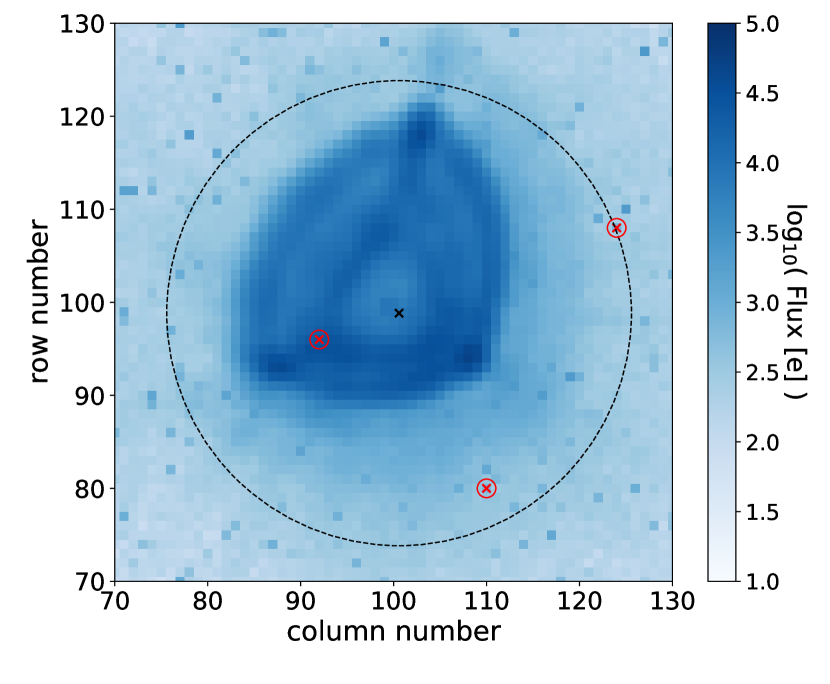
Figure 2: Extraction of $60\times 60$ arcsec of the CHEOPS FoV during the third visit centered on TOI-561. The dashed black circle represents the RINF photometric aperture surrounding the CHEOPS PSF, whose centroid is marked by the black cross. The positions of the three identified telegraphic pixels, including the one located within the CHEOPS PSF (see Appendix A), are highlighted by the red, circled crosses.

Finally, a variety of non-astrophysical sources, such as varying background, nearby contaminants or others, can produce short-term photometric trends in the CHEOPS light curves on the timescale of one orbit, due to the rotation of the CHEOPS FoV around the target and due to the nature of the spacecraft orbit. To correct for these effects, we detrended the light curves using the basis vectors provided by the DRP, as detailed in Section 5. The resulting detrended light curves are shown in Figure 3.

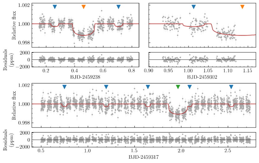
Figure 3: CHEOPS detrended light curves of TOI-561. Visits $1$, $2$ and $3$ are shown in the top left, top right, and bottom panel, respectively. The best-fitting model is over-plotted as a red solid line, and residuals are shown for each visit. The transits of planets b, c, and d are highlighted with blue, orange, and green triangles, respectively.

3.3 HARPS-N spectroscopy

In addition to the $82$ RVs published in L21, we collected $62$ high-resolution spectra using HARPS-N at the Telescopio Nazionale Galileo (TNG), in La Palma (Cosentino et al., 2012, 2014). These were used to refine the planetary masses and confirm the system configuration. The new observations were collected between 15 November 2020 and 1 June 2021. Following the same strategy of the previous season (L21), in addition to $30$ single observations, we collected six points per night on 8 and 10 February 2021, and two points per night on ten additional nights, specifically targeting the USP planet. The exposure time for all the observations was set to $1800$ s, resulting in a signal-to-noise ratio (SNR) at $550$ nm of $83\pm 20$ (median $\pm$ standard deviation) and a radial velocity measurement uncertainty of $1.0\pm 0.4$ m s^-1. All the observations were gathered with the second HARPS-N fibre illuminated by the Fabry–Perot calibration lamp to correct for the instrumental RV drift.

We reduced the global HARPS-N data set ($144$ RVs in total) using the new version of the HARPS-N Data Reduction Software based on the ESPRESSO pipeline (DRS, version 2.3.1; see Dumusque et al. 2021 for more details). We used a G2 flux template to correct for variations in the flux distribution as a function of wavelength, and a G2 binary mask to compute the cross-correlation function (CCF, Baranne et al. 1996; Pepe et al. 2002). We report the RVs and the associated activity indices (see Section 4.2) with their $1\sigma$ uncertainties in Table 5. As in L21, we removed from the first season data set five RVs with associated errors $>2.5$ m s^-1 from spectra with SNR $<35$ (see Appendix B in L21). All the RV uncertainties of the second season data set were below $2.5$ m s^-1, so no points were removed.

Table 5: HARPS-N radial velocity and activity indices measurements.

BJDTDB	RV	$\sigma_{\rm RV}$	FWHM	$\sigma_{\rm FWHM}$	BIS	$\sigma_{\rm BIS}$	Contrast	$\sigma_{\rm contr}$	S-index	$\sigma_{\text{S}}$	H$\alpha$	$\sigma_{\text{H}\alpha}$
$($d$)$	(m s-1)	(m s-1)	(km s-1)	(km s-1)	(m s-1)	(m s-1)					(dex)	(dex)
2458804.70780	79695.97	1.13	6.415	0.002	-86.82	2.26	59.879	0.021	0.1643	0.0005	0.2101	0.0002
2458805.77552	79699.66	0.85	6.419	0.002	-85.13	1.71	59.810	0.016	0.1702	0.0003	0.2124	0.0001
2458806.76769	79697.50	0.91	6.415	0.002	-83.66	1.82	59.861	0.017	0.1689	0.0003	0.2082	0.0001
…	…	…	…	…	…	…	…	…	…	…	…	…
This table is available in its entirety in machine-readable form.

3.4 HIRES spectroscopy

We included in our analysis $60$ high-resolution spectra collected with the W.M. Keck Observatory HIRES instrument on Mauna Kea, Hawaii between May 2019 and October 2020. The data set was published in W21, and we refer to that paper for details regarding the observing and data reduction procedures. The HIRES data set has an RMS of $5$ m s^-1, and a median individual RV uncertainty of $1.4$ m s^-1 (W21).

4 Probing the system architecture

4.1 CHEOPS confirmation of TOI-561 d

To solve the discrepancy among the planetary architectures proposed by L21 and W21 (Section 2.2), we initially looked for the transits of TOI-561 d ($\sim 25$ d) and TOI-561 f ($\sim 16$ d) in the TESS sector $35$ light curve, whereas TOI-561 e ($\sim 77$ d) was not expected to transit during those TESS observations. However, as shown in the top panel of Figure 4, the transits of planet d and f occurred during the light curve gap (Section 3.1), and so we could not use the new TESS data to conclusively discriminate between the two planetary configurations. Nonetheless, these observations ruled out the planet f alias at $\sim 8.1$ d mentioned in W21, since no transit events were detected at its predicted transit times.

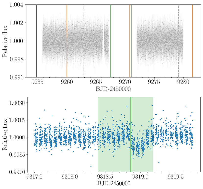
Figure 4: Top: 2-min cadence detrended TESS light curve of sector 35. The predicted transit times of TOI-561 c and d (according to L21 ephemeris), and TOI-561 f (according to W21 ephemeris), are highlighted with orange, green and black vertical solid lines, respectively. The black dashed lines indicate the predicted position of planet f alias at $\sim 8.1$ d. The only transit present in the light curve is the one of TOI-561 c at $\sim 9260$  BJD$-2450000$, while no transit events occurred at the predicted times of planet f alias. The transits of planet d and f fall into the time series gap. Bottom: CHEOPS visit scheduled to observe TOI-561 d. The green vertical solid line indicates the predicted transit time used to compute the CHEOPS observing window after the ephemeris update (Section 4.1). The transit occurred within the 68 per cent highest probability density interval, highlighted by the pale green region. We note that this transit is not consistent with the ephemeris propagation of planet f, which would have transited at $9319.94$ BJD$-2450000$, so almost one day after the observed CHEOPS transit.

We therefore decided to probe the L21 scenario collecting a transit of TOI-561 d using CHEOPS. We opted for the scheduling of the last seasonal observing window, in April, in order to take advantage of the most updated ephemeris to optimize the scheduling. For this reason, we performed a global fit adding to the literature data a partial set of the new HARPS-N RVs, as of 16 March 2021, and including the TESS sector $35$ light curve extracted from the second data release of the tica FFIs in March 2021. Even if no transit was detected, the new TESS sector helped to reduce the time window in which to search. In fact, the TESS data partially covered the $3\sigma$-uncertainty transit window, enabling us to exclude some time-spans in the computation of the CHEOPS visit. Thanks to the ephemeris update, the CHEOPS $3\sigma$ observing window shrank from $\sim 7.4$ d to $\sim 2.2$ d, demonstrating the importance of the early TESS data releases in the scheduling of follow-up observations. The bottom panel of Figure 4 shows the CHEOPS visit scheduled to observe TOI-561 d, whose transit occurred almost exactly at the predicted time, so confirming the planetary period and giving further credence to the 4-planet scenario proposed by L21 .

Even updating the ephemeris using the partial new HARPS-N data set, the last possible CHEOPS observing window of TOI-561 e in the 2021 season was still longer than seven days because of ephemeris uncertainties. Even including the full set of RVs would have not helped as the target was no longer observable with CHEOPS when the HARPS-N campaign finished. Given the high pressure on the CHEOPS schedule, we therefore plan the TOI-561 e observations for the 2022 observing season. The ephemeris for the 2022 CHEOPS observations will be updated using the TESS Sectors 45 and 46 observations in Nov-Dec 2021, and the results will be presented in a future publication.

4.2 Additional signals in the RV data

Before proceeding with the global modelling, we analyzed the RV data sets in order to confirm the robustness of the L21 scenario and search for potential new signals. The $\ell_{1}$-periodogram (Hara et al., 2017) of the combined HARPS-N and HIRES RVs (Figure 5) shows four significant peaks corresponding to the planetary periods reported in L21, plus hints of a possible longer period signal with a broad peak around $400-600$ days. We investigated the presence of this additional signal in a Bayesian framework using PyORBIT (Malavolta et al., 2016, 2018), a package for light curve and RVs analysis. We employed the dynesty nested-sampling algorithm (Skilling, 2004, 2006; Speagle, 2020), assuming $1000$ live points, and including offset and jitter terms for each data set. We first performed a 4-planet fit of the combined data sets, using the L21 values to impose Gaussian priors on periods and transit times, and assuming eccentric orbits with a half-Gaussian zero-mean prior on the eccentricity (with variance $0.098$; Van Eylen et al. 2019), except for the circular orbit of the USP planet. We let the semi-amplitude $K$ vary between $0.01$ and $100$ m s^-1. As can be seen in Figure 6, the RV residuals show an anomalous positive variation at $\sim 9000$ BJD-$2450000$, and the Generalized Lomb-Scargle (GLS, Zechmeister & Kürster 2009) periodogram of the RV residuals revealed the presence of a significant, broad peak at low frequencies. Moreover, the HARPS-N jitter was $1.84$ m s^-1, which is unusually high when compared to the value reported in L21 ($\sigma_{\rm HARPS-N}=1.29\pm 0.23$ m s^-1). We therefore performed a second fit including a fifth Keplerian signal, allowing the period to span between $2$ and $900$ d. According to the Bayesian Evidence, this model is strongly favoured with respect to the 4-planet model, with a difference in the logarithmic evidences $\Delta\ln\mathcal{Z}=19.0$ (Kass & Raftery, 1995). Moreover, the HARPS-N jitter decreased to $\sim 1.37$ m s^-1. After this fit, the periodogram of the residuals did not show evidence of additional significant peaks (Figure 6). This is confirmed also by the comparison with a 6-Keplerian model that we tested, with the period of the sixth Keplerian free to span between $2$ and $900$ d, whose Bayesian Evidence differed by less than $2$ from the 5-Keplerian model one, indicating that there was no strong evidence to favour a more complex model (Kass & Raftery, 1995).

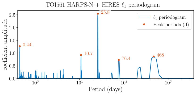
Figure 5: $\ell_{1}$-periodogram of the combined HARPS-N and HIRES data sets, computed on a grid of frequencies from $0$ to $2.5$ cycles per day. The total time-span of the observations is $768$ days. The code automatically accounts for the offset between HARPS-N and HIRES data by using the mean value of each data set.

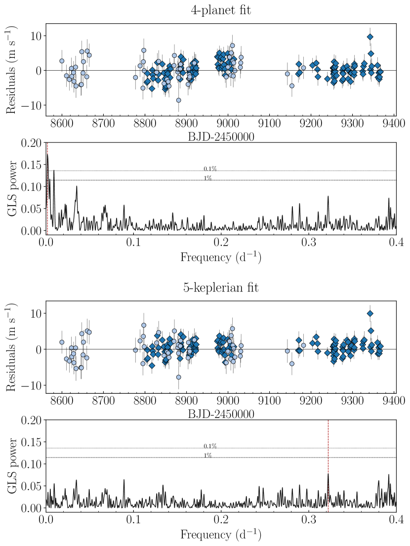
Figure 6: Time series and GLS periodogram of the RV residuals after the 4-planet and 5-Keplerian fits as described in Section 4.2. In the residuals plot, the HARPS-N and HIRES RVs are plotted with dark blue diamonds and light blue circles, respectively. In the periodogram plots, the dashed and dotted horizontal lines show the $1$ and $0.1$ per cent False Alarm Probability (FAP) level, respectively. The red vertical line indicates the main peak of each periodogram. The long-period peak around frequencies $0.0017-0.0025$ d^-1 ($P=400-600$ d) in the 4-planet residuals periodogram is modelled by the fifth Keplerian, and no more significant peaks are identified in the 5-Keplerian residuals periodogram. Moreover, the positive variation at $\sim 9000$ BJD-2450000 in the 4-planet fit residuals disappears in the 5-Keplerian fit residuals.

The fitted period of the fifth Keplerian was $\sim 480$ d. Such a long-term signal could be induced either by stellar activity, considering that stellar magnetic fields related to magnetic cycles can show variability on timescales of the order of $1-3$ years (e.g. Collier Cameron 2018; Hatzes 2019; Crass et al. 2021), or by an additional long-period planet. We refer here to an eventual long-period planet because, given the inferred semi-amplitude of $\sim 2$ m s^-1 (Table 6), an external companion with mass equal to $13$ $M_{\rm j}$ (assuming this value to be the threshold between planetary and sub-stellar objects) would have an inclination of $\sim 0.03$ deg. Such an inclination would imply an almost perpendicular orbit with respect to the orbital plane of the four inner planets, hinting at a very unlikely configuration. Therefore, in the hypothesis of the presence of an external companion, it would most likely be a planetary-mass object.
On one hand, all the five signals, including the long-term one, are recovered in an independent analysis that we performed with the CCF-based scalpels algorithm (Collier Cameron et al., 2021). Concisely, scalpels projects the RV time series onto the highest variance principal components of the time series of autocorrelation functions of the CCF, with the aim of distinguishing RV variations caused by orbiting planets from activity-induced distortions on each CCF. The absence of the signal in the scalpels shape-driven velocities indicates that the long-term periodicity is not due to shape changes in the line profiles, supporting the idea of a planetary origin. Moreover, TOI-561 is not expected to be a particularly active star given its old age and low $\log{\rm R}^{\prime}_{\rm HK}$, as assessed in the L21 and W21 activity analyses. As can be seen in Figure 7, the GLS periodogram of the majority of the activity indicators extracted with the HARPS-N DRS, i.e. full width at half maximum (FWHM), bisector span (BIS), contrast and H_α, do not show significant peaks, with none of them exceeding the $0.1$ False Alarm Probability (FAP) threshold, which we computed using a bootstrap approach, at the frequency of interest. On the other hand, the periodogram of the S-index, which is particularly sensitive to magnetically-induced activity, shows a significant, broad peak at low frequencies, potentially suggesting that the previously identified long-term variability is related to stellar activity. Considering this, we performed an additional dynesty fit assuming a 4-planet model and including a Gaussian Process (GP) regression with a quasi-periodic kernel, as formulated in Grunblatt et al. (2015), to account for the long-term signal. We modelled simultaneously the RVs and the S-index time series in order to better inform the GP (Langellier et al., 2021; Osborn et al., 2021), using two independent covariance matrices for each dataset with common GP hyper-parameters except for the amplitude of the covariance matrix, assuming uniform, non-informative priors on all of them. The fit suggests a periodicity longer than $\sim 570$ d, but the GP model is too flexible to derive a precise period value, considering also that the global RV baseline ($\sim 768$ d) is comparable with the periodicity of the long-term signal. The inferred semi-amplitudes of the four known planets differed by less than $0.07\sigma$ from the 5-Keplerian model ones, indicating that the different modelling of the long-term signal is not influencing the results for the known, transiting planets. Finally, as in the case of the 5-Keplerian fit, the HARPS-N jitter is significantly improved ($\sigma_{\rm HARPS-N}\sim 1.30$ m s^-1) when including the GP model. Therefore, since our Bayesian analyses showed that the modelling of the long-term signal is necessary to obtain the best picture of the system, we decided to perform the global fit assuming a 5-Keplerian model, but without drawing conclusions on the origin of the fifth signal. We stress that the 5-Keplerian fit does not provide absolute evidence of the presence of a fifth planet, since also poorly sampled stellar activity could be well modelled using a Keplerian (Pepe et al., 2013; Mortier & Collier Cameron, 2017; Affer et al., 2016), especially in our case where the RV baseline is of the order of the signal periodicity. Since it is not possible to distinguish a true planetary signal from an activity signal that has not been observed long enough to exhibit a loss of coherence in its phase or amplitude, only a follow-up campaign over several years can allow one to better understand the nature of this long-term signal.

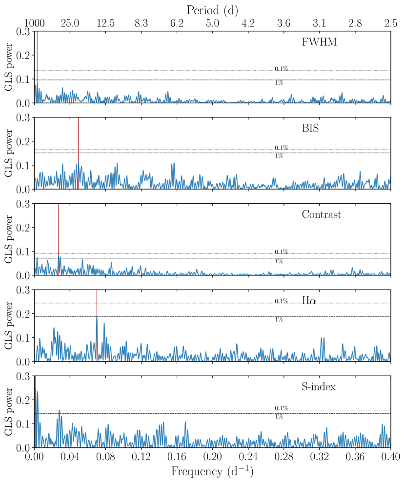
Figure 7: GLS periodogram of the HARPS-N activity indices. The main peak of each periodogram is highlighted with a red vertical line. The dashed and dotted horizontal lines indicate the $1$ and $0.1$ per cent FAP levels, respectively. The only peak above the $0.1$ FAP level is the low-frequency peak in the S-index periodogram, as discussed in Section 4.2.

5 Joint photometric and RV analysis

To infer the properties of the TOI-561 planets, we jointly modelled all photometric and spectroscopic data with PyORBIT, using PyDE + emcee (Foreman-Mackey et al., 2013) as described in Section 5 of L21, and adopting the same convergence criteria. We ran $96$ chains (twice the number of the model parameters) for $250000$ steps, discarding the first $50000$ as burn-in.

Based on the analysis presented in the previous section, we assumed a 5-Keplerian model, including four planets plus a fifth Keplerian with period free to span between $2$ to $900$ d. We fitted a common value for the stellar density, using the value reported in Table 1 as Gaussian prior. We adopted the quadratic limb-darkening law as parametrized by Kipping (2013), putting Gaussian priors on the $u_{1}$, $u_{2}$ coefficients, obtained for the TESS and CHEOPS passband through a bilinear interpolation of limb darkening profiles by Claret (2017) and Claret (2021) respectively, and assuming a $1\sigma$ uncertainty of $0.1$ for each coefficient. We imposed a half-Gaussian zero-mean prior (Van Eylen et al., 2019) on the planet eccentricities, except for the USP planet, whose eccentricity was fixed to zero. We assumed uniform priors for all the other parameters.

To model the long-term correlated noise in the TESS light curve, we included in the fit a GP regression with a Matérn-3/2 kernel against time, as shown in Figure 1, and we added a jitter term to account for possible extra white noise. We pre-decorrelated the CHEOPS light curves with the pycheops package (Maxted et al., 2021), selecting the detrending parameters according to the Bayes factor to obtain the best correlated noise model for each visit. For all the three CHEOPS visits, a decorrelation for the first three harmonics of the roll angle was necessary, plus first-order polynomials in time, x-y centroid position, and smearing. We then used the detrended light curves (Figure 3) for the global PyORBIT fit. In order to check if the detrending was affecting our results for the planetary parameters, we also performed an independent global analysis with the juliet package (Espinoza et al., 2019), including in the global modelling the basis vectors selected with pycheops to detrend the data simultaneously. All the results were consistent within $1\sigma$, indicating that the pre-detrending did not significantly alter our inferred results. Finally, for both the HARPS-N and HIRES data sets we included jitter and offset terms as free parameters.

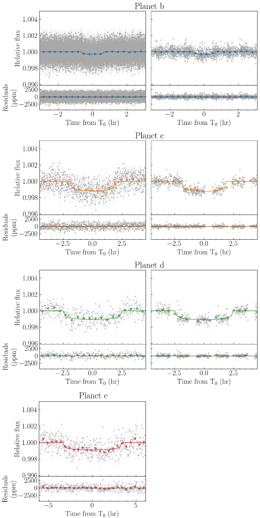
Figure 8: Phase-folded TESS (left) and CHEOPS (right) light curves of TOI-561 b, c, and d. Planet e shows a single transit in the TESS light curve, and it has no CHEOPS observations. For each planet, the coloured line indicates the best-fitting model, and residuals are shown in the bottom panels. Data points binned over $20$ min (planet b) and $30$ min (planets c, d and e) are shown with coloured dots.

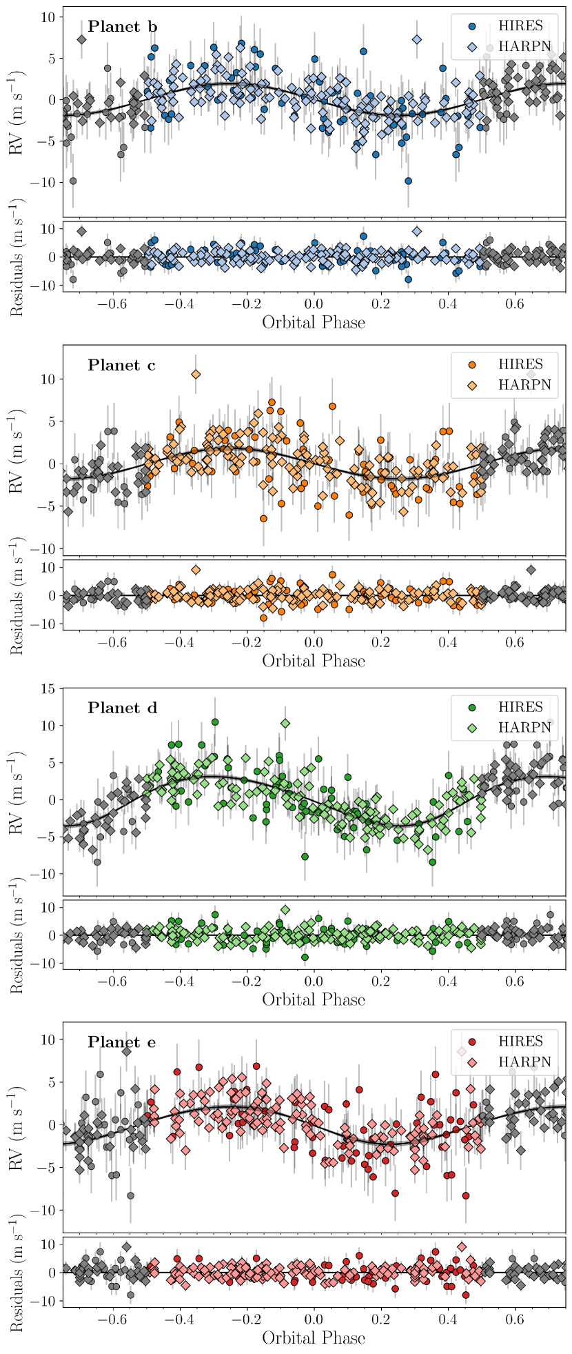
Figure 9: Phase-folded HARPS-N and HIRES RVs with residuals of TOI-561 b, c, d and e, as resulting from the joint photometric and spectroscopic fit. The error bars include the jitter term added in quadrature.

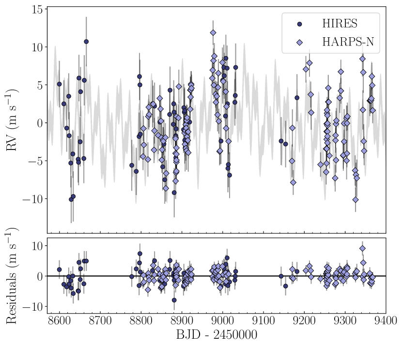
Figure 10: Global model (grey line) with residuals of HARPS-N and HIRES RVs according to the 5-Keplerian photometric and spectroscopic fit. The error bars include the jitter term added in quadrature.

We summarize our best-fitting model results in Table 6, and we show the transit model, phase-folded RVs and global RV model in Figures 8, 9, and 10, respectively. We inferred precise masses and radii for all the four planets in the system, whose positions in the mass-radius diagram are shown in Figure 11. With a radius of $R_{\rm b}=1.425\pm 0.037$ R_⊕ and a mass of $M_{\rm b}=2.00\pm 0.23$ M_⊕ (from $K_{\rm b}=1.93\pm 0.21$ m s^-1), TOI-561 b is located in a region of the mass-radius diagram which is not consistent with a pure rocky composition, as will be also shown in Section 6 by our internal structure modelling. Our analysis confirms TOI-561 b to be the lowest density ($\rho_{\rm b}=3.8\pm 0.5$ g cm^-3) USP planet known to date (Figure 12). In order to further confirm the planetary density, we also performed a specific RV analysis of TOI-561 b using the Floating Chunk Offset method (FCO; Hatzes 2014). The FCO analysis, detailed in Appendix B, confirms the low mass inferred for TOI-561 b, and consequently its low density. Thanks to the CHEOPS observations, we also improved significantly the radius of TOI-561 c, for which we obtained a value of $R_{\rm c}=2.91\pm 0.04$ R_⊕. From the semi-amplitude $K_{\rm c}=1.81_{-0.22}^{+0.23}$ m s^-1 we inferred a mass of $M_{\rm c}=5.39_{-0.68}^{+0.69}$ M_⊕, implying a density of $\rho_{\rm c}=1.2\pm 0.2$ g cm^-3. From the combined fit of one TESS and one CHEOPS transit, we inferred a radius of $2.82\pm 0.07$ R_⊕ for planet d, which has a mass of $M_{\rm c}=13.2_{-0.9}^{+1.0}$ M_⊕ (from $K_{\rm d}=3.34_{-0.22}^{+0.23}$ m s^-1) and a resulting density of $\rho_{\rm d}=3.2\pm 0.3$ g cm^-3. Finally, for TOI-561 e, which shows a single transit in TESS sector $8$, we derived a radius of $R_{\rm e}=2.55_{-0.13}^{+0.12}$ R_⊕, a mass of $M_{\rm e}=12.6\pm 1.4$ M_⊕, and an average density of $\rho_{\rm d}=4.2\pm 0.8$ g cm^-3. Lastly, the period inferred for the fifth Keplerian in the model was $473_{-25}^{+36}$ d, with a $7.2\sigma$ detected semi-amplitude of $1.94\pm 0.27$ m s^-1. As discussed in Section 4.2, additional data spanning a longer baseline are needed to definitively confirm the planetary nature of this long-term signal.

Table 6: Parameters of the TOI-561 system, including the fifth Keplerian signal, as determined from the joint photometric and spectroscopic fit described in Section 5.

[t] Planetary parameters TOI-561 b TOI-561 c TOI-561 d TOI-561 e $5^{\rm th}$ Keplerian $P$ (d) $0.4465688_{-0.0000008}^{+0.0000007}$ $10.778831_{-0.000036}^{+0.000034}$ $25.7124_{-0.0002}^{+0.0001}$ $77.03_{-0.24}^{+0.25}$ $473_{-25}^{+36}$ $T_{0}$ (TBJD)^a $2317.7498\pm 0.0005$ $2238.4629_{-0.0009}^{+0.0008}$ $2318.966_{-0.004}^{+0.003}$ $1538.180_{-0.005}^{+0.004}$ $1664_{-33}^{+28}$ $a/$$R_{\star}$ $2.685_{-0.025}^{+0.024}$ $22.43_{-0.21}^{+0.20}$ $40.04_{-0.37}^{+0.36}$ $83.22_{-0.79}^{+0.77}$ $279_{-10}^{+14}$ $a$ (AU) $0.0106\pm 0.0001$ $0.0884\pm 0.0009$ $0.158\pm 0.002$ $0.328\pm 0.003$ $1.1_{-0.4}^{+0.6}$ $R_{\mathrm{p}}/$$R_{\star}$ $0.0155\pm 0.0004$ $0.0316\pm 0.0004$ $0.0306\pm 0.0008$ $0.0278_{-0.0014}^{+0.0016}$ - $R_{\rm p}$ (R_⊕) $1.425\pm 0.037$ $2.91\pm 0.04$ $2.82\pm 0.07$ $2.55_{-0.13}^{+0.12}$ - $b$ $0.13_{-0.09}^{+0.10}$ $0.12_{-0.08}^{+0.13}$ $0.45_{-0.17}^{+0.11}$ $0.28_{-0.18}^{+0.15}$ - $i$ (deg) $87.2_{-2.1}^{+1.9}$ $89.69_{-0.31}^{+0.21}$ $89.40_{-0.11}^{+0.21}$ $89.80_{-0.10}^{+0.13}$ - $T_{14}$ (h) $1.31\pm 0.02$ $3.75_{-0.08}^{+0.05}$ $4.54_{-0.29}^{+0.32}$ $6.98_{-0.40}^{+0.24}$ - $e$ $0$ (fixed) $0.030_{-0.021}^{+0.035}$ $0.122_{-0.048}^{+0.054}$ $0.079_{-0.050}^{+0.058}$ $0.085_{-0.059}^{+0.083}$ $\omega$ (deg) $90$ (fixed) $291_{-84}^{+55}$ $235_{-26}^{+14}$ $143_{-44}^{+42}$ $348_{-53}^{+198}$ $K$ (m s^-1) $1.93\pm 0.21$ $1.81_{-0.22}^{+0.23}$ $3.34_{-0.22}^{+0.23}$ $2.19\pm 0.23$ $1.94\pm 0.27$ $M_{\rm p}$ (M_⊕) $2.00\pm 0.23$ $5.39_{-0.68}^{+0.69}$ $13.2_{-0.9}^{+1.0}$ $12.6\pm 1.4$ $20\pm 3\,^{b}$ $\rho_{\rm p}$ ($\rho_{\oplus}$) $0.69\pm 0.10$ $0.22\pm 0.03$ $0.59\pm 0.06$ $0.76\pm 0.14$ - $\rho_{\rm p}$ (g cm^-3) $3.8\pm 0.5$ $1.2\pm 0.2$ $3.2\pm 0.3$ $4.2\pm 0.8$ - $S_{\rm p}$ ($S_{\oplus}$) $4745\pm 269$ $68.2\pm 3.9$ $21.4\pm 1.3$ $4.96\pm 0.28$ - $T_{\rm eq}^{c}$ (K) $2310\pm 33$ $800\pm 11$ $598\pm 9$ $415\pm 6$ - $g_{\rm p}^{d}$ (m s^-2) $9.7\pm 1.2$ $6.2\pm 0.8$ $16.3\pm 1.5$ $19.0\pm 2.9$ - Common parameters $R_{\star}$^e (R_⊙) $0.843\pm 0.005$ $M_{\star}$^e (M_⊙) $0.806\pm 0.036$ $\rho_{\star}$ ($\rho_{\odot}$) $1.31\pm 0.05$ $u_{1,\mathrm{TESS}}$ $0.33\pm 0.08$ $u_{2,\mathrm{TESS}}$ $0.23\pm 0.09$ $u_{1,\mathrm{CHEOPS}}$ $0.46\pm 0.07$ $u_{2,\mathrm{CHEOPS}}$ $0.22\pm 0.09$ $\sigma_{\rm HARPS-N}^{\rm f}$ (m s^-1) $1.40_{-0.14}^{+0.15}$ $\sigma_{\rm HIRES}^{\rm f}$ (m s^-1) $2.77_{-0.31}^{+0.36}$ $\gamma^{\rm g}_{\rm HARPS-N}$ (m s^-1) $79700.41\pm 0.26$ $\gamma^{\rm g}_{\rm HIRES}$ (m s^-1) $-1.20\pm 0.42$

• ^a TESS Barycentric Julian Date (BJD$-2457000$). ^b Minimum mass in the hypothesis of a planetary origin. ^c Computed as $T_{\rm eq}=T_{\star}\,\biggl{(}\dfrac{R_{\star}}{2a}\biggr{)}^{1/2}\,[f(1-A_{\rm B})]^{1/4}$, assuming $f=1$ and a null Bond albedo ($A_{\rm B}=0$). ^d Planetary surface gravity. ^e As determined from the stellar analysis in Section 2.1. ^f RV jitter term. ^g RV offset.

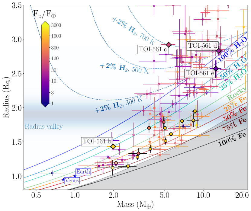
Figure 11: Mass-radius diagram for exoplanets with radii and masses measured with a precision better than $30$%, colour coded according to their incidental flux. Data are taken from the Extrasolar Planets Encyclopaedia catalogue (http://exoplanet.eu/catalog/) as of 18 October 2021. The TOI-561 planets are labelled, and highlighted with coloured diamonds. The USP planets are emphasized with thick, black-contoured circles. The theoretical mass-radius curves for various chemical compositions (Zeng et al., 2019) are represented by solid coloured lines, while the dashed lines indicate the curves for an Earth-like core surrounded by a H₂ envelope ($2$% mass fraction) at varying equilibrium temperatures. The forbidden region predicted by collisional stripping (Marcus et al., 2010) is marked by the shaded grey region.

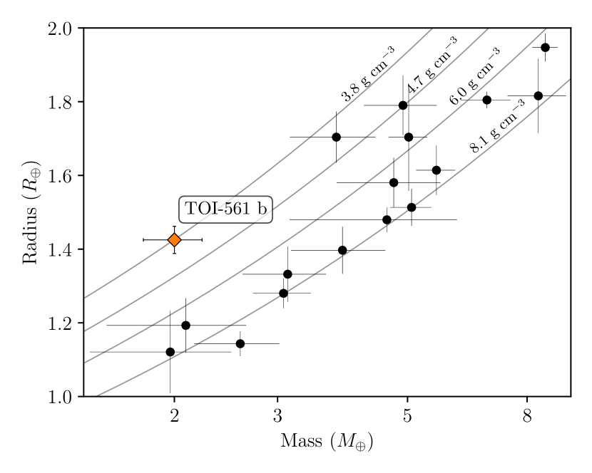
Figure 12: Mass-radius diagram of confirmed USP planets ($P<1$ d, $R_{\rm p}$< 2 R_⊕) as taken from the Extrasolar Planets Encyclopaedia catalogue in date 18 October 2021. Iso-density lines are plotted in grey. TOI-561 b stands out as the lowest density USP planet known to date ($\rho_{\rm b}=3.8\pm 0.5$ g cm^-3).

6 Internal structure modelling

We modelled the internal planetary structure in a Bayesian framework, following the procedure detailed in Leleu et al. (2021). Our model assumes fully-differentiated planets composed of four layers, comprising an iron and sulfur central core, a silicate mantle which includes Si, Mg and Fe, a water layer, and a pure H/He gas layer. The inner core is modelled assuming the Hakim et al. (2018) equation of state (EOS), the silicate mantle uses the Sotin et al. (2007) EOS, and the water layer uses the Haldemann et al. (2020) EOS. The core, mantle and water layer compose the ‘solid’ part of the planet. The thickness of the gas envelope is computed as a function of stellar age and irradiation, and mass and radius of the solid part, according to the model presented in Lopez & Fortney (2014). We assumed no compression effects of the gas envelope on the solid part, a hypothesis which is justified a posteriori given the low mass fraction of gas obtained for each planet (see below).

Our Bayesian model fits the planetary system as a whole, rather than performing an independent fit for each planet, in order to account for the correlations between the absolute planetary masses and radii, which depend on the stellar properties. The model fits the stellar (mass, radius, effective temperature, age, chemical abundances of Fe, Mg, Si), and planetary properties (RV semi-amplitudes, transit depths, orbital periods) to derive the posterior distributions of the internal structure parameters. The internal structure parameters modelled for each planet are the mass fractions of the core, mantle and water layer, the mass of the gas envelope, the iron molar fraction in the core, the silicon and magnesium molar fraction in the mantle, the equilibrium temperature and the age of the planet (equal to the age of the star). For a more extensive discussion on the relation among input data and derived parameters we refer to Leleu et al. (2021). We assumed the mass fraction of the inner core, mantle, and water layer to be uniform on the simplex (the surface on which they add up to one), with the water mass fraction having an upper boundary of 0.5 (Thiabaud et al., 2014; Marboeuf et al., 2014). For the mass of the gas envelope, we assumed a uniform prior in logarithmic space. Finally, we assumed the Si/Mg/Fe molar ratios of each planet to be equal to the stellar atmospheric values (even though Adibekyan et al. (2021a) recently showed that the stellar and planetary abundances may not be always correlated in a one-to-one relation). We emphasize the fact that, as in many Bayesian analyses, the results presented below in terms of planet internal structure depend to some extent on the selection of the priors, which we chose following i.e. Dorn et al. (2017), Dorn et al. (2018), and Leleu et al. (2021). Analysing the same data with very different priors (e.g. non uniform core/mantle/water mass fraction or gas fraction uniform in linear scale) would lead to different conclusions.

We show the results of the internal structure modelling for the four planets in Figure 13. As expected from its closeness to the host star, planet b has basically no H/He envelope, while the other three planets show a variable amount of gas mass. Planet c hosts a relatively massive gaseous envelope, with a gas mass of (5 and 95 per cent quantiles) $M_{\rm gas,c}=0.07_{-0.02}^{+0.04}$ M_⊕ ($1.3_{-0.4}^{+0.8}$ weight percent wt%). Planet d hosts the most massive envelope ($M_{\rm gas,d}=0.10_{-0.07}^{+0.13}$ M_⊕), which, considering the total mass of the planet, correspond to a smaller relative mass fraction of $0.8_{-0.5}^{+1.0}$ wt%, while TOI-561 e’s envelope spans a range between $-10.7<\log M_{\rm gas,e}<-1.0$, implying an upper limit on the gas mass of $0.11$ M_⊕ ($<0.9$ wt%). As expected from its low density, TOI-561 b could host a significant amount of water, having a water mass of $M_{\rm H_{2}O,b}=0.62_{-0.44}^{+0.32}$ M_⊕ ($31_{-22}^{+16}$ wt%). We stress that this result is highly dependent on the caveat of including only a solid water layer in the model. In fact, a massive water layer, if present on a planet with such a high equilibrium temperature, would imply the presence of a massive steam atmosphere (Turbet et al., 2020). This would in turn considerably change the inferred water mass fraction with respect to a model that includes only a solid water layer. Due to the presence of the gas envelope, the amount of water in both planet c and d is almost unconstrained ($M_{\rm H_{2}O,c}=1.29_{-1.14}^{+1.24}$ M_⊕, i.e. $24_{-21}^{+23}$ wt%; $M_{\rm H_{2}O,d}=3.56_{-3.18}^{+2.78}$ M_⊕, i.e. $27_{-24}^{+21}$ wt%), while TOI-561 e modelling points toward a massive water layer, with $M_{\rm H_{2}O,e}=4.50_{-3.65}^{+1.69}$ M_⊕ ($36_{-29}^{+13}$ wt%).

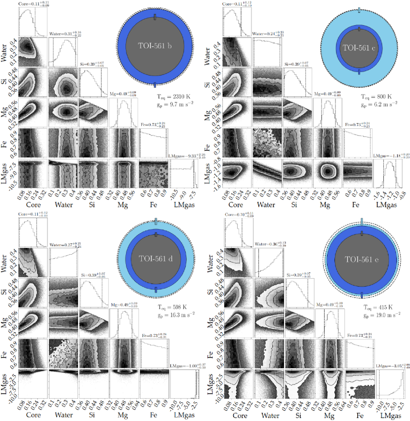
Figure 13: Posterior distributions of the main parameters describing the internal structure of TOI-561 b (top left), c (top right), d (bottom left), and e (bottom right). Each corner plot shows the mass fraction of the inner core and of the water layer, the molar fractions of silicon and magnesium in the mantle, the iron molar fraction in the inner core, and the mass of gas in logarithmic scale. On top of each column are printed the mean and the 5 per cent and 95 per cent quantiles values. For each planet, and we show an illustration of the radius fractions of the inner core+mantle (dark gray), water layer (dark blue), and gas envelope (light blue), corresponding to the medians of the posterior distributions. The coloured rectangles indicate the uncertainty on the corresponding layer thickness, while the black dashed outer rings represent the uncertainty on the total radius. Equilibrium temperature and planetary surface gravity are reported for each planet.

7 Atmospheric evolution

We employed the system parameters derived in this work to constrain the evolution of the stellar rotation period, which we use as a proxy for the evolution of the stellar high-energy emission affecting atmospheric escape, and the predicted initial atmospheric mass fraction of the detected transiting planets $f_{\rm atm}^{\rm start}$, that is the mass of the planetary atmosphere at the time of the dispersal of the protoplanetary disk. To this end, we used the planetary atmospheric evolution code Pasta described by Bonfanti et al. (2021a), which is an updated version of the original code presented by Kubyshkina et al. (2019b, a). The code models the evolution of the planetary atmospheres combining a model predicting planetary atmospheric escape rates based on hydrodynamic simulations (this has the advantage over other commonly used analytical estimates to account for both XUV-driven and core-powered mass loss; Kubyshkina et al., 2018), a model of the stellar high-energy (X-ray plus extreme ultraviolet; XUV) flux evolution (Bonfanti et al., 2021a), a model relating planetary parameters and atmospheric mass (Johnstone et al., 2015b), and stellar evolutionary tracks (Choi et al., 2016). The main assumptions of the framework are that planet migration did not occur after the dispersal of the protoplanetary disk, and that the planets hosted at some point in the past or still host a hydrogen-dominated atmosphere.

For each planet, the evolution calculations begin at an age of 5 Myr, which is the age assumed in the code for the dispersal of the protoplanetary disk. At each time step, the framework derives the mass-loss rate from the atmospheric escape model employing the stellar flux and the system parameters, and uses it to update the atmospheric mass fraction. This procedure is then repeated until the age of the system is reached or the planetary atmosphere has completely escaped. The free parameters of the algorithm are the initial atmospheric mass fraction at the time of the dispersal of the protoplanetary disk, and the indexes of the power law controlling the stellar rotation period (see Bonfanti et al., 2021a, for a detailed description of the mathematical formulation of the power law), that we use as proxy for the stellar XUV emission.

The free parameters are constrained by implementing the atmospheric evolution algorithm in a Bayesian framework employing the MCMC tool presented by Cubillos et al. (2017). The framework uses the system parameters with their uncertainties as input priors. It then computes millions of forward planetary evolutionary tracks, varying the input parameters according to the shape of the prior distributions, and varying the free parameters within pre-defined ranges, fitting the current planetary atmospheric mass fractions obtained as described in Section 6. The fit is done at the same time for all planets, thus simultaneously constraining the rotational period, and the results are posterior distributions of the free parameters. In particular, we opted for fitting for the planetary atmospheric mass fractions instead of the planetary radii. This enables the code to be more accurate by avoiding the continuous conversion of the atmospheric mass fraction into planetary radius, given the other system parameters (see also Delrez et al., 2021).

Figure 14 shows the results of the planetary atmospheric evolution simulations. As a proxy for the evolution of the stellar rotation period, in Figure 14, we show the posterior distribution of the stellar rotation period at an age of 150 Myr, further comparing it to the distribution of stellar rotation periods observed in stars member of young clusters of comparable age and with masses that deviate from $M_{\star}$ less than $0.1$ M_⊙ (from Johnstone et al., 2015a). The inferred posterior distribution for the rotation period is consistent with membership of the slowly-rotating period-colours sequence in clusters of this age. However, this comparison should be taken with some caution, since there are no comprehensive studies on the rotation-colour distributions of $150$ Myr-old clusters with the same metallicity as TOI-561. The initial atmospheric mass fractions of planets b and c are rather broad and peak at about one planetary mass. This is because both planets are close enough to the host star and have a small enough mass to have been subject to significant atmospheric escape. Therefore, to enable the presence of a thin hydrogen atmosphere, as predicted by the internal structure model, both planets had to host a significant hydrogen envelope after the formation and atmospheric accretion processes. Instead, planets d and e are far from the host star and massive enough not to have been subject to significant atmospheric escape, which is why we obtain an initial atmospheric mass fraction that resembles the current one. We also find that the posterior distributions of all input parameters match well the inserted priors (not shown here). As a whole, the results indicate that the currently observed system parameters are compatible with a scenario in which migration happened (if at all) exclusively inside the protoplanetary disk. Otherwise the code would have led to mismatches between the prior and posterior of the input parameters (particularly for what concerns the planetary masses and/or the stellar mass and age), in addition to showing incoherent results in the posterior distribution of the output parameters. This is for example the case of the TOI-1064 system, which is composed by two transiting planets with comparable masses and irradiation levels, but significantly different radii (Wilson et al., 2022). In our framework in which planets do not migrate after the dispersal of the protoplanetary nebula, reproducing the physical parameters of the planets composing the TOI-1064 system requires different evolutions of the stellar rotation rate, which is not possible, thus calling for a post-nebula migration.

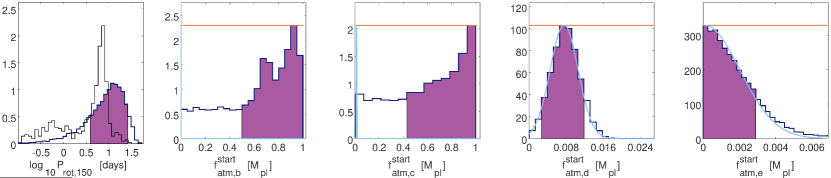
Figure 14: From left to right: Posterior distributions (dark blue lines) of the stellar rotation period at an age of $150$ Myr and of the initial atmospheric mass fractions of TOI-561 b, c, d and e. In each panel, the purple region represents the $68$ per cent highest probability density intervals. In the left panel, the black thin line shows the rotation period distribution of stars member of open clusters with ages around $150$ Myr. Data are taken from Johnstone et al. (2015a), who report the rotation period of $\sim\,2000$ stars belonging to the Pleiades, M50, M35, and NGC 2516, whose ages are between $125$ and $150$ Myr. To generate the black histogram we selected a sub-sample of $578$ stars, which have masses that deviate from $M_{\star}$ less than $0.1$ M_⊙. In the other panels, the horizontal orange lines mark the uniform prior used in the fit, scaled to the highest peak of each posterior distribution for better visualization. The light blue lines indicate the current atmospheric mass fraction of each planet determined as described in Section 6.

8 Discussion and conclusions

In this study, we confirm the presence of four transiting planets around TOI-561, with orbital periods of approximately $0.44$, $10.8$, $25.7$, and $77$ days (Table 6). Our analysis disproves the presence of the previously suggested planet TOI-561 f ($P\sim 16.3$ day; W21). TOI-561 is one of the few 4-planet systems having precise radius and mass measurements for all the planets. Thanks to our global photometric and RV analysis, we refined all masses and radii with respect to the L21 values, and we precisely determined the planetary bulk densities, with uncertainties of $14.4$%, $13.6$%, $10.2$%, and $18.4$% for planets b, c, d, and e, respectively. The higher uncertainty on planet e reflects the lower precision in the radius determination ($5$% uncertainty), which is based on the analysis of a single TESS transit, and highlights the importance of the high-precision CHEOPS photometry. In fact, with a single CHEOPS transit we managed to decrease the uncertainty on the radius of planet d from $5.1$% (L21, based on one TESS transit) to $2.5$%. Including also the improvement on the mass, this implied a decrease on the density uncertainty from $18.9$% to $10.2$%. We expect a similar improvement for planet e with future CHEOPS observations scheduled for 2022. The improvement in the radius of TOI-561 e is particularly important, since the planet is an interesting target for the study of the internal structure of cold sub-Neptunes. Its long period ($P_{\rm d}=77.03_{-0.24}^{+0.25}$ d) implies an insolation flux of $S_{\rm e}=4.96\pm 0.28$ $S_{\oplus}$ and a relatively cool zero Bond albedo equilibrium temperature of $T_{\rm eq,e}=415\pm 6$ K. As shown in Figure 15, TOI-561 e is one of the few cool, long-period planets orbiting a star bright enough for precise RV characterization, and it is therefore an optimal test-case to refine tools and models that will be useful to characterize targets of future long-staring missions like PLATO.

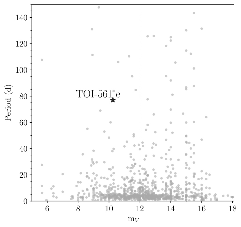
Figure 15: $V$ magnitude versus planetary periods for confirmed transiting exoplanets as reported in the Extrasolar Planets Encyclopaedia catalogue (http://exoplanet.eu/catalog/) in date 18 October 2021. The dashed vertical line marks $V=12$ mag. TOI-561 e is one of the few long-period planets orbiting a star bright enough for precise RV characterization.

TOI-561 hosts one of the most intriguing USP planets discovered to date. As initially suggested by L21, our analysis confirms that TOI-561 b is the lowest density ($\rho_{\mathrm{b}}=3.8\pm 0.5$ g cm^-3) USP super-Earth that we know of (see Figure 12), and it paves the way for in-depth studies of interior composition, and formation and evolution processes of USP planets. Even though now the mass values are consistent within $1\sigma$, contrary to what proposed by W21 (see Section 2.2) TOI-561 b is not consistent with a pure rocky composition, and to explain the planetary density our internal structure modelling (Section 6) predicts basically no H/He envelope, and a massive water layer. In this regard, an important point to consider is that, with an insolation flux of $S_{\rm b}\simeq 4745$ $S_{\oplus}$, the planet receives more irradiation from the star than the theoretical runaway greenhouse limit (Kasting et al., 1993; Goldblatt & Watson, 2012; Kopparapu et al., 2013). In this case, a large water content would imply the presence of an extended steam atmosphere, which in turn would increase the measured radius with respect to a purely condensed water world, leading in our model to an overestimation of the bulk water content (Turbet et al., 2020). The presence of a water steam envelope could eventually be tested with the James Webb Space Telescope (JWST). In fact, with an Emission Spectroscopy Metric (ESM, Kempton et al. 2018) value of $8.2$, TOI-561 b is a promising target for secondary eclipse and phase curve observations. More complex models, including a lighter core compositions (i.e. a Ca/Al enriched core), the modelling of water steam envelopes, or wet-melt solid interiors related to deep water reservoirs (Dorn & Lichtenberg, 2021), could be an interesting step forward in the understanding of the planet structure and composition. The low density of TOI-561 b could also be related to the fact that the host star is a metal-poor, thick-disk star. Adibekyan et al. (2021a) showed that the composition of the rocky planets reflects the chemical abundances of the host star (even though not in a one-to-one relation), so implying a lighter composition for TOI-561 b with respect to other USP planets that orbit more metal-rich stars. According to Adibekyan et al. (2021a), the low density of TOI-561 b is consistent with the general $\rho$/$\rho_{\rm Earth-like}$ – $f_{\rm iron}^{\rm star}$ trend and dispersion inferred from the sample of rocky planets analysed by the authors (see Figs. 2, 3 therein), where $\rho$/$\rho_{\rm Earth-like}$ is the planetary density normalised to that expected for an Earth-like composition, and $f_{\rm iron}^{\rm star}$ is the iron-to-silicate mass fraction of the protoplanetary disk as inferred from the stellar properties. An additional interesting remark concerns the Galactic kinematics of the host star. According to our analysis, performed as described in Mustill et al. (2021), TOI-561 is located in a low-density region of the 6-dimensional Galactic phase space (see Winter et al. 2020, Mustill et al. 2021, and Kruijssen et al. 2021 for definition and discussion), which is not surprising given that TOI-561 is a thick disk star (Mustill et al., 2021). Kruijssen et al. (2020) showed that stars in low-density regions seem to host no super-Earths, but only sub-Neptunes, i.e. planets having a significant H/He envelope and therefore located above the radius gap. In this context, TOI-561 b is an interesting object that runs counter to this finding. We point out that this result should be taken with some caution, since the Kruijssen et al. (2020) sample does not include planets with periods shorter than one day, and it excludes stars with ages $>4.5$ Gyr.

All the four planets seem to host a large water layer (Section 6), although with high uncertainties, especially for planet c and d, due to the degeneracy related to the possible presence of a gas envelope. Also in this case, the presence of a considerable amount of water could be linked with the stellar properties. In fact, Santos et al. (2017) showed that metal-poor, thick disk stars are expected to form planetary building blocks with a higher water mass fraction ($\sim 76$%) compared to metal-rich, thin disk stars ($\sim 58$%). Therefore, we would expect these stars to produce water-rich planets, a result that is in agreement with our findings on the TOI-561 system.

Except for TOI-561 b, all the other planets are suggested to host a non-negligible H/He envelope. In particular, the gas content of planet c ($\sim 1.3$ wt%, the highest mass fraction among the four planets) implies a much lower density with respect to the density of planet d, even though the two planets have a similar size. This is reflected in the different positions of the planets in the mass-radius diagram (Figure 11). The two planets show hints of a different evolution for what concerns their gas content. In fact, our atmospheric evolution model (Section 7) suggests that planet c underwent a strong envelope loss after the atmospheric accretion and the dispersal of the protoplanetary nebula, while planet d (as well as planet e) did not experience strong atmospheric escape, with a current gas content that is comparable to the original one. The surprising difference in gas mass fraction between planets c, d and e, not only at present time but also at the end of their formation phase, takes probably its origin in the conditions that prevailed during the protoplanetary disk phase. Planet c is indeed likely sub-critical because of its low mass, where sub-critical planets are those with masses below the critical value required to initiate runaway gas accretion (see Helled et al. 2014 for a recent review on the core accretion model), whereas planets d and e never accreted large amounts of gas as demonstrated in Section 7, and so they also remained always below the critical mass. The interpretation of the different gas mass fractions could therefore result from the structure of sub-critical planets. In this case, the gas mass fraction depends on the core mass, the thermodynamical properties in the disk, and more importantly the accretion rate of solids (lower accretion rate translating in larger gas mass fraction). Interpreting the internal structure of the four planets of the system in a global planetary system formation model could therefore constrain these parameters.

With its derived properties, TOI-561 c has a Transmission Spectroscopy Metric (TSM, Kempton et al. 2018) of $110.4$, and is therefore a suitable target for atmospheric characterization with JWST. Instead, planets d and e have lower TSM values of $30.7$ and $16.2$, respectively. As the TSM is proportional to the equilibrium temperature, it is not surprising to obtain lower values for the two planets, given their longer periods.

In addition to the characterization of the four planets, we also identified a significant long-term signal ($P\sim 473$ d) in the RVs. On the basis of our current dataset, we are not able to distinguish between a stellar (magnetically-induced) or planetary origin. Long-term monitoring using both spectroscopic ground-based facilities and future long-staring missions like the PLATO spacecraft will allow us to shed light on the nature of this additional signal, and to potentially find new outer companions. It is worth noting that, if the above-mentioned signal proves in future to be of planetary origin, there is a non-zero chance that, under the assumption of co-planarity, such a planet would transit. In fact, assuming the same inclination of planet e and using the semi-major axis $a/\mbox{$R_{\star}$}=279_{-10}^{+14}$ derived from our global fit, we infer an impact parameter of $0.97_{-0.63}^{+0.49}$. Moreover, the planet would orbit in TOI-561’s empirical habitable zone ($175\lesssim P\lesssim 652$ d), as originally defined by Kasting et al. (1993) using a 1D climate model, and later updated in Kopparapu et al. (2013); Ramirez & Kaltenegger (2016) for main-sequence stars with $2600<$ $T_{{\rm eff}}$ $<10000$ K.

This work bears witness to the fruitful results that can be obtained by the timely combination of data coming from different instruments. It adds to the works (Bonfanti et al., 2021b; Leleu et al., 2021; Delrez et al., 2021) that prove the potential of CHEOPS in precisely characterizing TESS-discovered exoplanets, as well as demonstrating the key role of high-precision spectrographs such as HARPS-N when working in synergy with space-based facilities.

Data Availability

HARPS-N observations and data products are available through the Data & Analysis Center for Exoplanets (DACE) at https://dace.unige.ch/. TESS data products can be accessed through the official NASA website https://heasarc.gsfc.nasa.gov/docs/tess/data-access.html. All underlying data are available either in the appendix/online supporting material or will be available via VizieR at CDS.

Appendix A CHEOPS light curves and telegraphic pixel treatment

As described in Section 3.2, the three CHEOPS visits of TOI-561 were reduced via the standard DRP processing. The light curves presented in this study, obtained using the RINF aperture size (RINF $=0.9\,\times$ DEFAULT, where DEFAULT = $25$ px; see also Section 3.2), are shown in Figure 16. While for the two initial visits the automatic DRP processes was performed, the appearance of some telegraphic pixels during the third visit required a more in-depth analysis.

In addition to the large number of known hot pixels present in the CHEOPS CCD (some of them visible in Figure 2), some normal pixels can change their behaviour during the duration of a visit, for example becoming ‘hot’ after a SAA crossing. These pixels, called ‘telegraphic’ for their abnormal behaviour, can affect the photometry if located within the photometric aperture (see for example Leleu et al. 2021). During the third CHEOPS visit, we identified an unusual flux bump before the ingress of TOI-561 d transit, at BJD $\sim 2459318.75$ (top panel, Figure 17). After analyzing the statistics of each pixel light curve within the photometric aperture, we detected a telegraphic pixel with a large flux variation (second panel, Figure 17) located within the CHEOPS PSF. The exact position of this pixel on the CHEOPS CCD is shown in Figure 2. We masked the pixel flux and repeated the photometric extraction of the visit using the RINF aperture, so removing the flux jump in the light curve (bottom panel, Figure 17). During this analysis, we detected two additional telegraphic pixels within the photometric aperture, inducing smaller, but still significant variations in the light curve flux (third panel, Figure 17). We corrected for the effect of these pixels as described above.

While investigating the nature of the flux bump happening during the third visit, we also extracted the light curve using a PSF-photometry approach exploiting the PIPE (PSF Imagette Photometric Extraction) software. PIPE is a photometric extraction package specifically developed to extract CHEOPS light curves by applying PSF photometry on the $60$-pixel imagettes, complementing the offical DRP extraction. The use of PSF photometry makes usually easier to filter out the impact of hot pixels and cosmic rays, by either giving them a lower weight or masking them entirely in the fitting process. However, in this case the telegraphic pixel was located inside the CHEOPS PSF, requiring a careful manual masking. As for the DRP light curve, the flux bump in the PIPE photometry is reduced after masking the telegraphic pixel (bottom panel, Figure 18). The PIPE-extracted light curve resulted in a slightly lower mean absolute deviation (MAD) with respect to the DRP photometry (top panel, Figure 18), mainly due to the lower number of outliers present in the PSF photometry. For a more detailed comparison between PIPE and DRP photometries, see Morris et al. (2021b). We performed the same global analysis described in Section 5 using the PIPE light curve instead of the DRP one, obtaining consistent results and comparable uncertainties on the transit parameters of both planets b and d. We therefore decided to use the light curve obtained with the official DRP extraction in our final analysis.

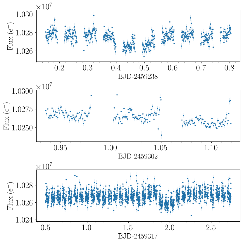
Figure 16: CHEOPS RINF light curves of TOI-561 as extracted from the DRP, with $4\sigma$-clipping for outliers removal. Visits $1$, $2$ and $3$ are shown from top to bottom.

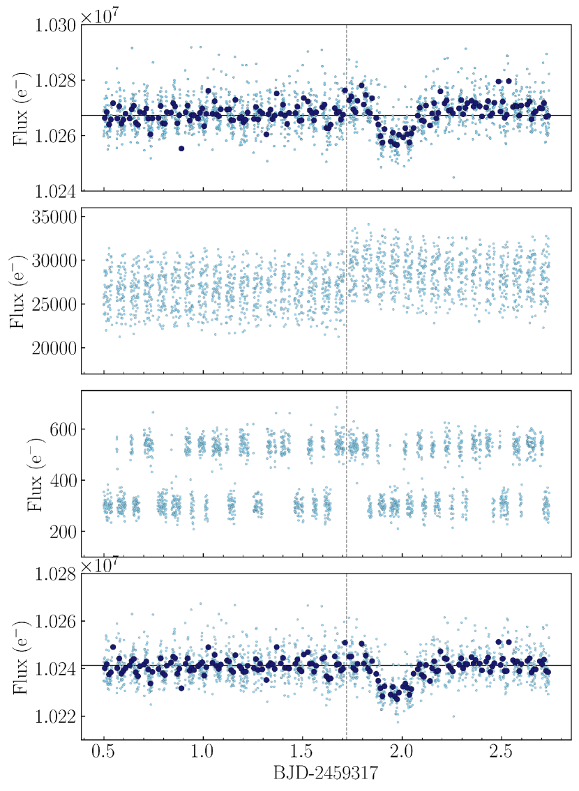
Figure 17: Top panel: TOI-561 RINF original light curve of the third visit (light blue dots) after the removal of $4\sigma$ outliers, with over-plotted the $15$-minute binned light curve (dark blue dots). The start of the flux jump due to the telegraphic pixel is marked with the dashed vertical line. Second panel: light curve of the telegraphic pixel located within the CHEOPS PSF. Third panel: light curve of the two additional telegraphic pixels located within the RINF aperture. Bottom panel: corrected light curve after masking the three telegraphic pixels.

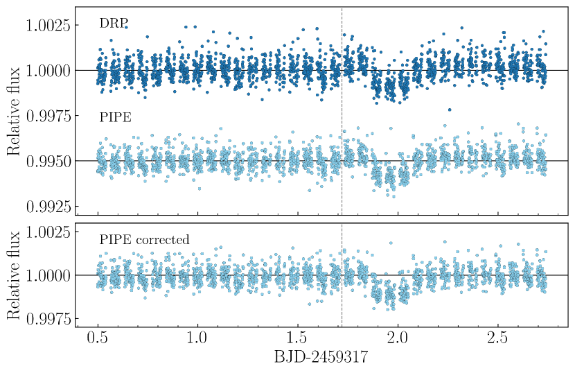
Figure 18: Top panel: comparison between DRP and PIPE-extracted light curve of TOI-561 third visit, before the telegraphic pixel correction and with $4\sigma$ outliers removal. The DRP has an MAD of $371$ ppm over the whole visit, while PIPE of $325$ ppm. Bottom panel: PIPE light curve after the telegraphic pixel correction. The light curve gets slightly noisier (MAD $=331$ ppm) because one less pixel is considered in the reduction, but more reliable thanks to the exclusion of the telegraphic pixel flux. In both panels, the beginning of the flux jump is highlighted with a vertical dashed line.

Appendix B Floating Chunk Offset method on TOI-561 b

In order to investigate the literature discrepancy on the mass of TOI-561 b (Section 2.2), we adopted a specific observing strategy with HARPS-N targeting the USP planet (Section 3.3), obtaining multiple observations during the same night for $22$ nights. Multiple nightly observations can be used to precisely infer the mass of USP planets using the Floating Chunk Offset method (FCO; Hatzes 2014), which consists in applying a nightly offset to remove all the other signals present in the system, both of planetary and stellar origin (i.e. Howard et al. 2013; Pepe et al. 2013; Malavolta et al. 2018; Frustagli et al. 2020). The FCO method is only applicable when the separation between the USP period and the period of all the other signals is large enough, and the RV semi-amplitude has a similar or larger value with respect to the other signals. As demonstrated in L21, these conditions apply to TOI-561 b, for which the authors derived an FCO semi-amplitude of $K_{\rm b,FCO}=1.80\pm 0.38$ m s^-1 ($M_{\rm b,FCO}=1.83\pm 0.39$ M_⊕) exploiting multiple observations collected over ten nights.

Here, we applied the FCO method to TOI-561 b on a total of $22$ HARPS-N nights, adding $12$ novel nights to the $10$ nights already presented in L21. Out of the total set, four nights have six multiple observations extending over more than $40$ per cent of the orbital period of the planet, and span opposite orbital phases to provide an optimal phase coverage. We performed a PyDE + emcee fit with PyORBIT, assuming a fixed zero eccentricity and Gaussian priors on period and $T_{0}$ coming from the global fit, and we added a jitter term to account for possible additional white noise. We derived a semi-amplitude of $K_{\rm b}=1.81\pm 0.31$ m s^-1, corresponding to a mass of $M_{\rm b}=1.86\pm 0.33$ M_⊕, with a jitter of $0.96_{-0.23}^{+0.25}$ m s^-1. Figure 19 shows the resulting phase-folded RVs. The derived mass and semi-amplitude are nicely in agreement with the L21 values, and they support the values inferred from our joint photometric and RV modelling (Section 5), being consistent within $1\sigma$. Given the higher number of RVs included in the joint fit, which led to smaller uncertainties on the derived parameters, we decided to adopt as final values for TOI-561 b the ones obtained from the global modelling, i.e. $K_{\rm b}=1.93\pm 0.21$ m s^-1, $M_{\rm b}=1.99\pm 0.22$ M_⊕.

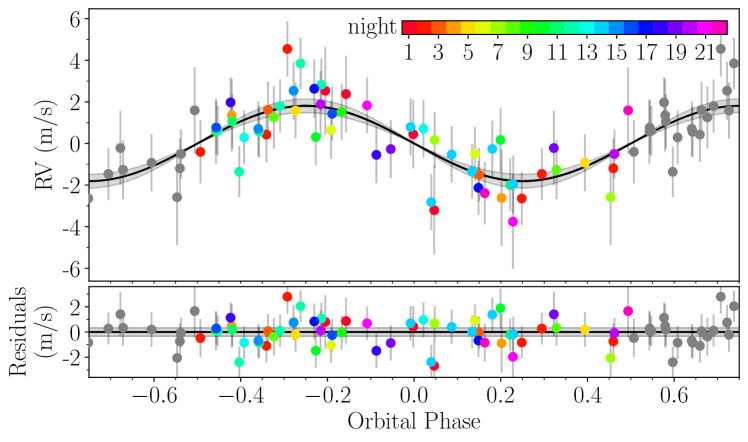
Figure 19: Phase-folded RVs of the $22$ HARPS-N nights used to model TOI-561 b with the FCO method. The error bars include the jitter term added in quadrature.

Affiliations

¹ Dipartimento di Fisica e Astronomia "Galileo Galilei", Università degli Studi di Padova, Vicolo dell’Osservatorio 3, 35122 Padova, Italy
² INAF, Osservatorio Astronomico di Padova, Vicolo dell’Osservatorio 5, 35122 Padova, Italy
³ Centre for Exoplanet Science, SUPA School of Physics and Astronomy, University of St Andrews, North Haugh, St Andrews KY16 9SS, UK
⁴ Physikalisches Institut, University of Bern, Gesellsschaftstrasse 6, 3012 Bern, Switzerland
⁵ Center for Space and Habitability, Gesellsschaftstrasse 6, 3012 Bern, Switzerland
⁶ Astrophysics Group, Cavendish Laboratory, University of Cambridge, J.J. Thomson Avenue, Cambridge CB3 0HE, UK
⁷ Kavli Institute for Cosmology, University of Cambridge, Madingley Road, Cambridge CB3 0HA, UK
⁸ Space Research Institute, Austrian Academy of Sciences, Schmiedlstrasse 6, A-8042 Graz, Austria
⁹ Astrophysics Group, University of Exeter, Exeter EX4 2QL, UK
¹⁰ Aix Marseille Univ, CNRS, CNES, LAM, 38 rue Frédéric Joliot-Curie, 13388 Marseille, France
¹¹ Department of Astronomy, University of Geneva, Chemin Pegasi 51, Versoix, Switzerland
¹² Department of Physics and Kavli Institute for Astrophysics and Space Research, Massachusetts Institute of Technology, Cambridge, MA 02139, USA
¹³ Department of Astronomy, University of Wisconsin-Madison, Madison, WI 53706, USA
¹⁴ Center for Astrophysics | Harvard and Smithsonian, 60 Garden Street, Cambridge, MA 02138, USA
¹⁵ SUPA, Institute for Astronomy, University of Edinburgh, Blackford Hill, Edinburgh EH9 3HJ, Scotland, UK
¹⁶ Centre for Exoplanet Science, University of Edinburgh, Edinburgh EH93FD, UK
¹⁷ Department of Astronomy, Stockholm University, AlbaNova University Center, 10691 Stockholm, Sweden
¹⁸ Fundación Galileo Galilei - INAF, Rambla J. A. F. Perez, 7, E-38712 S.C. Tenerife, Spain
¹⁹ INAF – Osservatorio Astronomico di Brera, via E. Bianchi 46, I-23807 Merate (LC), Italy
²⁰ Instituto de Astrofisica e Ciencias do Espaco, Universidade do Porto, CAUP, Rua das Estrelas, 4150-762 Porto, Portugal
²¹ INAF - Osservatorio Astrofisico di Torino, Via Osservatorio 20, I-10025 Pino Torinese, Italy
²² Space sciences, Technologies and Astrophysics Research (STAR) Institute, Université de Liège, Allée du 6 Août 19C, 4000 Liège, Belgium
²³ University of Southern Queensland, Centre for Astrophysics, West Street, Toowoomba, QLD 4350 Australia
²⁴ Lund Observatory, Dept. of Astronomy and Theoretical Physics, Lund University, Box 43, 22100 Lund, Sweden
²⁵ Instituto de Astrofisica de Canarias, 38200 La Laguna, Tenerife, Spain
²⁶ Departamento de Astrofísica, Universidad de La Laguna, E-38206 La Laguna, Tenerife, Spain
²⁷ Institut de Ciencies de l’Espai (ICE, CSIC), Campus UAB, Can Magrans s/n, 08193 Bellaterra, Spain
²⁸ Institut d’Estudis Espacials de Catalunya (IEEC), 08034 Barcelona, Spain
²⁹ Admatis, 5. Kandó Kálmán Street, 3534 Miskolc, Hungary
³⁰ Depto. de Astrofisica, Centro de Astrobiologia (CSIC-INTA), ESAC campus, 28692 Villanueva de la Cañada (Madrid), Spain
³¹ Departamento de Fisica e Astronomia, Faculdade de Ciencias, Universidade do Porto, Rua do Campo Alegre, 4169-007 Porto, Portugal
³² Université Grenoble Alpes, CNRS, IPAG, 38000 Grenoble, France
³³ DTU Space, National Space Institute, Technical University of Denmark, Elektrovej 328, DK-2800 Kgs. Lyngby, Denmark
³⁴ Institute of Planetary Research, German Aerospace Center (DLR), Rutherfordstrasse 2, 12489 Berlin, Germany
³⁵ Université de Paris, Institut de physique du globe de Paris, CNRS, F-75005 Paris, France
³⁶ Centre for Mathematical Sciences, Lund University, 22100 Lund, Sweden
³⁷ Astrobiology Research Unit, Université de Liège, Allée du 6 Août 19C, B-4000 Liège, Belgium
³⁸ Department of Astronomy, Stockholm University, SE-106 91 Stockholm, Sweden
³⁹ Leiden Observatory, University of Leiden, PO Box 9513, 2300 RA Leiden, The Netherlands
⁴⁰ Department of Space, Earth and Environment, Chalmers University of Technology, Onsala Space Observatory, 43992 Onsala, Sweden
⁴¹ Dipartimento di Fisica, Università degli Studi di Torino, via Pietro Giuria 1, I-10125, Torino, Italy
⁴² Department of Astrophysics, University of Vienna, Tuerkenschanzstrasse 17, 1180 Vienna, Austria
⁴³ Division Technique INSU, CS20330, 83507 La Seyne sur Mer cedex, France
⁴⁴ Department of Physics, University of Warwick, Gibbet Hill Road, Coventry CV4 7AL, United Kingdom
⁴⁵ Science and Operations Department - Science Division (SCI-SC), Directorate of Science, European Space Agency (ESA), European Space Research and Technology Centre (ESTEC), Keplerlaan 1, 2201-AZ Noordwijk, The Netherlands
⁴⁶ NASA Ames Research Center, Moffett Field, CA 94035, USA
⁴⁷ Konkoly Observatory, Research Centre for Astronomy and Earth Sciences, 1121 Budapest, Konkoly Thege Miklós út 15-17, Hungary
⁴⁸ ELTE Eötvös Loránd University, Institute of Physics, Pázmány Péter sétány 1/A, 1117 Budapest, Hungary
⁴⁹ IMCCE, UMR8028 CNRS, Observatoire de Paris, PSL Univ., Sorbonne Univ., 77 av. Denfert-Rochereau, 75014 Paris, France
⁵⁰ Institut d’astrophysique de Paris, UMR7095 CNRS, Université Pierre & Marie Curie, 98bis blvd. Arago, 75014 Paris, France
⁵¹ Astrophysics Group, Keele University, Staffordshire, ST5 5BG, United Kingdom
⁵² INAF - Osservatorio Astronomico di Palermo, Piazza del Parlamento 1, I-90134 Palermo, Italy
⁵³ INAF - Osservatorio Astronomico di Cagliari, Via della Scienza 5, I-09047, Selargius, Italy
⁵⁴ Komaba Institute for Science, The University of Tokyo, 3-8-1 Komaba, Meguro, Tokyo 153-8902, Japan
⁵⁵ Astrobiology Center, 2-21-1 Osawa, Mitaka, Tokyo 181-8588, Japan
⁵⁶ INAF, Osservatorio Astrofisico di Catania, Via S. Sofia 78, 95123 Catania, Italy
⁵⁷ P&P Software GmbH, High Tech Center, Taegerwilen, CH-8274, Switzerland
⁵⁸ Institute of Optical Sensor Systems, German Aerospace Center (DLR), Rutherfordstrasse 2, 12489 Berlin, Germany
⁵⁹ ESTEC, European Space Agency, 2201AZ, Noordwijk, NL
⁶⁰ Center for Astronomy and Astrophysics, Technical University Berlin, Hardenbergstrasse 36, 10623 Berlin, Germany
⁶¹ Institut für Geologische Wissenschaften, Freie Universität Berlin, 12249 Berlin, Germany
⁶² Department of Earth, Atmospheric, and Planetary Sciences, Massachusetts Institute of Technology, Cambridge, MA 02139, USA
⁶³ Department of Aeronautics and Astronautics, Massachusetts Institute of Technology, Cambridge, MA 02139, USA
⁶⁴ ELTE Eötvös Loránd University, Gothard Astrophysical Observatory, 9700 Szombathely, Szent Imre h. u. 112, Hungary
⁶⁵ MTA-ELTE Exoplanet Research Group, 9700 Szombathely, Szent Imre h. u. 112, Hungary
⁶⁶ SETI Institute, Mountain View, CA 94043, USA
⁶⁷ Institute of Astronomy, University of Cambridge, Madingley Road, Cambridge, CB3 0HA, United Kingdom
⁶⁸ Department of Astrophysical Sciences, Princeton University, 4 Ivy Lane, Princeton, NJ 08544, USA

References

- Adams et al. (2020) Adams F. C., Batygin K., Bloch A. M., Laughlin G., 2020, MNRAS, 493, 5520
- Adibekyan et al. (2021a) Adibekyan V., et al., 2021a, Science, 374, 330–332
- Adibekyan et al. (2021b) Adibekyan V., et al., 2021b, A&A, 649, A111
- Affer et al. (2016) Affer L., et al., 2016, A&A, 593, A117
- Baglin et al. (2006) Baglin A., et al., 2006, in 36th COSPAR Scientific Assembly. p. 3749
- Bailer-Jones et al. (2021) Bailer-Jones C. A. L., Rybizki J., Fouesneau M., Demleitner M., Andrae R., 2021, VizieR Online Data Catalog, p. I/352
- Baranne et al. (1996) Baranne A., et al., 1996, A&AS, 119, 373
- Barros et al. (2022) Barros S. C. C., Akinsanm B., Boué G., Smith A. M. S., Laskar J., Ulmer-Moll S., Lillo-Box J., the CHEOPS Team 2022, arXiv e-prints, p. arXiv:2201.03328
- Benz et al. (2021) Benz W., et al., 2021, Experimental Astronomy, 51, 109
- Blackwell & Shallis (1977) Blackwell D. E., Shallis M. J., 1977, Monthly Notices of the Royal Astronomical Society, 180, 177
- Bonfanti & Gillon (2020) Bonfanti A., Gillon M., 2020, A&A, 635, A6
- Bonfanti et al. (2015) Bonfanti A., Ortolani S., Piotto G., Nascimbeni V., 2015, A&A, 575, A18
- Bonfanti et al. (2016) Bonfanti A., Ortolani S., Nascimbeni V., 2016, A&A, 585, A5
- Bonfanti et al. (2021a) Bonfanti A., Fossati L., Kubyshkina D., Cubillos P. E., 2021a, arXiv e-prints, p. arXiv:2110.09106
- Bonfanti et al. (2021b) Bonfanti et al., 2021b, A&A, 646, A157
- Borsato et al. (2021) Borsato L., et al., 2021, MNRAS, 506, 3810
- Borucki et al. (2010) Borucki W. J., et al., 2010, Science, 327, 977
- Buchhave et al. (2012) Buchhave L. A., et al., 2012, Nature, 486, 375
- Buchhave et al. (2014) Buchhave L. A., et al., 2014, Nature, 509, 593
- Castelli & Kurucz (2003) Castelli F., Kurucz R. L., 2003, in Piskunov N., Weiss W. W., Gray D. F., eds, IAU Symposium Vol. 210, Modelling of Stellar Atmospheres. p. A20 (arXiv:astro-ph/0405087)
- Choi et al. (2016) Choi J., Dotter A., Conroy C., Cantiello M., Paxton B., Johnson B. D., 2016, ApJ, 823, 102
- Ciardi et al. (2013) Ciardi D. R., Fabrycky D. C., Ford E. B., Gautier T. N. I., Howell S. B., Lissauer J. J., Ragozzine D., Rowe J. F., 2013, ApJ, 763, 41
- Claret (2017) Claret A., 2017, A&A, 600, A30
- Claret (2021) Claret A., 2021, Research Notes of the American Astronomical Society, 5, 13
- Collier Cameron (2018) Collier Cameron A., 2018, The Impact of Stellar Activity on the Detection and Characterization of Exoplanets. Springer International Publishing, Cham, pp 1791–1799, doi:10.1007/978-3-319-55333-7_23, https://doi.org/10.1007/978-3-319-55333-7_23
- Collier Cameron et al. (2021) Collier Cameron A., et al., 2021, MNRAS, 505, 1699
- Cosentino et al. (2012) Cosentino R., et al., 2012, in Society of Photo-Optical Instrumentation Engineers (SPIE) Conference Series. p. 1, doi:10.1117/12.925738
- Cosentino et al. (2014) Cosentino R., et al., 2014, in Society of Photo-Optical Instrumentation Engineers (SPIE) Conference Series. p. 8, doi:10.1117/12.2055813
- Crass et al. (2021) Crass J., et al., 2021, Extreme Precision Radial Velocity Working Group Final Report (arXiv:2107.14291)
- Cubillos et al. (2017) Cubillos P., Harrington J., Loredo T. J., Lust N. B., Blecic J., Stemm M., 2017, AJ, 153, 3
- Cutri et al. (2003) Cutri R. M., et al., 2003, VizieR Online Data Catalog, 2246
- Dai et al. (2021) Dai F., et al., 2021, The Astronomical Journal, 162, 62
- Deline et al. (2022) Deline A., et al., 2022, arXiv e-prints, p. arXiv:2201.04518
- Delrez et al. (2021) Delrez L., et al., 2021, Nature Astronomy, 5, 775
- Dorn & Lichtenberg (2021) Dorn C., Lichtenberg T., 2021, arXiv e-prints, p. arXiv:2110.15069
- Dorn et al. (2017) Dorn C., Venturini, Julia Khan, Amir Heng, Kevin Alibert, Yann Helled, Ravit Rivoldini, Attilio Benz, Willy 2017, A&A, 597, A37
- Dorn et al. (2018) Dorn C., Mosegaard K., Grimm S. L., Alibert Y., 2018, ApJ, 865, 20
- Dumusque et al. (2021) Dumusque X., et al., 2021, A&A, 648, A103
- Espinoza et al. (2019) Espinoza N., Kossakowski D., Brahm R., 2019, MNRAS, 490, 2262
- Fabrycky et al. (2014) Fabrycky D. C., et al., 2014, The Astrophysical Journal, 790, 146
- Fausnaugh et al. (2020) Fausnaugh M. M., Burke C. J., Ricker G. R., Vanderspek R., 2020, Research Notes of the American Astronomical Society, 4, 251
- Foreman-Mackey et al. (2013) Foreman-Mackey D., Hogg D. W., Lang D., Goodman J., 2013, PASP, 125, 306
- Frustagli et al. (2020) Frustagli G., et al., 2020, A&A, 633, A133
- Gaia Collaboration et al. (2018) Gaia Collaboration et al., 2018, A&A, 616, A1
- Gaia Collaboration et al. (2021) Gaia Collaboration et al., 2021, A&A, 649, A1
- Goldblatt & Watson (2012) Goldblatt C., Watson A. J., 2012, Philosophical Transactions of the Royal Society of London Series A, 370, 4197
- Grunblatt et al. (2015) Grunblatt S. K., Howard A. W., Haywood R. D., 2015, ApJ, 808, 127
- Guenther et al. (2017) Guenther E. W., et al., 2017, preprint, (arXiv:1705.04163)
- Hakim et al. (2018) Hakim K., Rivoldini A., Van Hoolst T., Cottenier S., Jaeken J., Chust T., Steinle-Neumann G., 2018, Icarus, 313, 61
- Haldemann et al. (2020) Haldemann Alibert, Yann Mordasini, Christoph Benz, Willy 2020, A&A, 643, A105
- Hara et al. (2017) Hara N. C., Boué G., Laskar J., Correia A. C. M., 2017, Monthly Notices of the Royal Astronomical Society, 464, 1220
- Hatzes (2014) Hatzes A. P., 2014, A&A, 568, A84
- Hatzes (2019) Hatzes A. P., 2019, The Doppler Method for the Detection of Exoplanets. 2514-3433, IOP Publishing, doi:10.1088/2514-3433/ab46a3, http://dx.doi.org/10.1088/2514-3433/ab46a3
- Helled et al. (2014) Helled R., et al., 2014, in Beuther H., Klessen R. S., Dullemond C. P., Henning T., eds, Protostars and Planets VI. p. 643 (arXiv:1311.1142), doi:10.2458/azu_uapress_9780816531240-ch028
- Hooton et al. (2021) Hooton M. J., et al., 2021, arXiv e-prints, p. arXiv:2109.05031
- Howard et al. (2013) Howard A. W., et al., 2013, Nature, 503, 381
- Howell et al. (2014) Howell S. B., et al., 2014, PASP, 126, 398
- Hoyer et al. (2020) Hoyer S., Guterman P., Demangeon O., Sousa S. G., Deleuil M., Meunier J. C., Benz W., 2020, A&A, 635, A24
- Jenkins (2020) Jenkins J. M., 2020, Kepler Data Processing Handbook, Kepler Science Document KSCI-19081-003, https://archive.stsci.edu/kepler/documents.html
- Jenkins et al. (2016) Jenkins J. M., et al., 2016, in Chiozzi G., Guzman J. C., eds, Society of Photo-Optical Instrumentation Engineers (SPIE) Conference Series Vol. 9913, Software and Cyberinfrastructure for Astronomy IV. SPIE, pp 1232 – 1251, doi:10.1117/12.2233418, https://doi.org/10.1117/12.2233418
- Jiang et al. (2020) Jiang C.-F., Xie J.-W., Zhou J.-L., 2020, AJ, 160, 180
- Johnstone et al. (2015a) Johnstone C. P., Güdel M., Brott I., Lüftinger T., 2015a, A&A, 577, A28
- Johnstone et al. (2015b) Johnstone C. P., et al., 2015b, ApJ, 815, L12
- Kass & Raftery (1995) Kass R. E., Raftery A. E., 1995, Journal of the American Statistical Association, 90, 773
- Kasting et al. (1993) Kasting J. F., Whitmire D. P., Reynolds R. T., 1993, Icarus, 101, 108
- Kempton et al. (2018) Kempton E. M. R., et al., 2018, PASP, 130, 114401
- Kipping (2013) Kipping D. M., 2013, MNRAS, 435, 2152
- Kopparapu et al. (2013) Kopparapu R. K., et al., 2013, ApJ, 765, 131
- Kruijssen et al. (2020) Kruijssen J. M. D., Longmore S. N., Chevance M., 2020, ApJ, 905, L18
- Kruijssen et al. (2021) Kruijssen J. M. D., Longmore S. N., Chevance M., Laporte C. F. P., Motylinski M., Keller B. W., Henshaw J. D., 2021, arXiv e-prints, p. arXiv:2109.06182
- Kubyshkina et al. (2018) Kubyshkina D., et al., 2018, A&A, 619, A151
- Kubyshkina et al. (2019a) Kubyshkina D., et al., 2019a, A&A, 632, A65
- Kubyshkina et al. (2019b) Kubyshkina D., et al., 2019b, ApJ, 879, 26
- Lacedelli et al. (2021) Lacedelli G., et al., 2021, MNRAS, 501, 4148 (L21)
- Langellier et al. (2021) Langellier N., et al., 2021, AJ, 161, 287
- Leleu et al. (2021) Leleu et al., 2021, A&A, 649, A26
- Lendl et al. (2020) Lendl M., et al., 2020, A&A, 643, A94
- Lindegren et al. (2021) Lindegren L., et al., 2021, A&A, 649, A4
- Lissauer et al. (2011) Lissauer J. J., et al., 2011, The Astrophysical Journal Supplement Series, 197, 8
- Lopez & Fortney (2014) Lopez E. D., Fortney J. J., 2014, The Astrophysical Journal, 792, 1
- Malavolta et al. (2016) Malavolta L., et al., 2016, A&A, 588, A118
- Malavolta et al. (2017) Malavolta L., Lovis C., Pepe F., Sneden C., Udry S., 2017, MNRAS, 469, 3965
- Malavolta et al. (2018) Malavolta L., et al., 2018, AJ, 155, 107
- Marboeuf et al. (2014) Marboeuf Thiabaud, Amaury Alibert, Yann Cabral, Nahuel Benz, Willy 2014, A&A, 570, A36
- Marcus et al. (2010) Marcus R. A., Sasselov D., Stewart S. T., Hernquist L., 2010, ApJ, 719, L45
- Marigo et al. (2017) Marigo et al., 2017, The Astrophysical Journal, 835, 77
- Maxted et al. (2021) Maxted P. F. L., et al., 2021, arXiv e-prints, p. arXiv:2111.08828
- Mayor & Queloz (1995) Mayor M., Queloz D., 1995, Nature, 378, 355
- Millholland et al. (2017) Millholland S., Wang S., Laughlin G., 2017, ApJ, 849, L33
- Mills et al. (2019) Mills S. M., Howard A. W., Petigura E. A., Fulton B. J., Isaacson H., Weiss L. M., 2019, AJ, 157, 198
- Morris et al. (2021a) Morris B. M., et al., 2021a, arXiv e-prints, p. arXiv:2106.07443
- Morris et al. (2021b) Morris Heng, Kevin Brandeker, Alexis Swan, Andrew Lendl, Monika 2021b, A&A, 651, L12
- Mortier & Collier Cameron (2017) Mortier A., Collier Cameron A., 2017, A&A, 601, A110
- Mortier et al. (2014) Mortier A., Sousa S. G., Adibekyan V. Z., Brandão I. M., Santos N. C., 2014, A&A, 572, A95
- Mustill et al. (2021) Mustill A. J., Lambrechts M., Davies M. B., 2021, arXiv e-prints, p. arXiv:2103.15823
- Osborn et al. (2021) Osborn H. P., et al., 2021, MNRAS, 502, 4842
- Pepe et al. (2002) Pepe F., Mayor M., Galland F., Naef D., Queloz D., Santos N. C., Udry S., Burnet M., 2002, A&A, 388, 632
- Pepe et al. (2013) Pepe F., et al., 2013, Nature, 503, 377
- Prieto-Arranz et al. (2018) Prieto-Arranz J., et al., 2018, A&A, 618, A116
- Ramirez & Kaltenegger (2016) Ramirez R. M., Kaltenegger L., 2016, ApJ, 823, 6
- Ricker et al. (2014) Ricker G. R., et al., 2014, Journal of Astronomical Telescopes, Instruments, and Systems, 1, 1
- Salmon et al. (2021) Salmon S. J. A. J., Van Grootel V., Buldgen G., Dupret M. A., Eggenberger P., 2021, A&A, 646, A7
- Sanchis-Ojeda et al. (2015) Sanchis-Ojeda R., et al., 2015, The Astrophysical Journal, 812, L11
- Santos et al. (2017) Santos N. C., et al., 2017, A&A, 608, A94
- Schanche et al. (2020) Schanche N., et al., 2020, MNRAS, 499, 428
- Scuflaire et al. (2008) Scuflaire R., Théado S., Montalbán J., Miglio A., Bourge P. O., Godart M., Thoul A., Noels A., 2008, Ap&SS, 316, 83
- Skilling (2004) Skilling J., 2004, in Fischer R., Preuss R., Toussaint U. V., eds, American Institute of Physics Conference Series Vol. 735, Bayesian Inference and Maximum Entropy Methods in Science and Engineering: 24th International Workshop on Bayesian Inference and Maximum Entropy Methods in Science and Engineering. pp 395–405, doi:10.1063/1.1835238
- Skilling (2006) Skilling J., 2006, Bayesian Anal., 1, 833
- Skrutskie et al. (2006) Skrutskie M. F., et al., 2006, AJ, 131, 1163
- Smith et al. (2012) Smith J. C., et al., 2012, PASP, 124, 1000
- Sotin et al. (2007) Sotin C., Grasset O., Mocquet A., 2007, Icarus, 191, 337
- Sousa (2014) Sousa S. G., 2014, [arXiv:1407.5817],
- Speagle (2020) Speagle J. S., 2020, MNRAS, 493, 3132
- Stassun et al. (2018) Stassun K. G., et al., 2018, The Astronomical Journal, 156, 102
- Stumpe et al. (2012) Stumpe M. C., et al., 2012, PASP, 124, 985
- Stumpe et al. (2014) Stumpe M. C., Smith J. C., Catanzarite J. H., Van Cleve J. E., Jenkins J. M., Twicken J. D., Girouard F. R., 2014, PASP, 126, 100
- Swayne et al. (2021) Swayne M. I., et al., 2021, MNRAS, 506, 306
- Szabó et al. (2021) Szabó G. M., et al., 2021, arXiv e-prints, p. arXiv:2108.02149
- Thiabaud et al. (2014) Thiabaud A., Marboeuf U., Alibert Y., Cabral N., Leya I., Mezger K., 2014, A&A, 562, A27
- Turbet et al. (2020) Turbet M., Bolmont E., Ehrenreich D., Gratier P., Leconte J., Selsis F., Hara N., Lovis C., 2020, A&A, 638, A41
- Van Eylen et al. (2019) Van Eylen V., et al., 2019, AJ, 157, 61
- Van Grootel et al. (2021) Van Grootel V., et al., 2021, A&A, 650, A205
- Weiss et al. (2018) Weiss L. M., et al., 2018, AJ, 156, 254
- Weiss et al. (2021) Weiss L. M., et al., 2021, AJ, 161, 56 (W21)
- Wilson et al. (2022) Wilson T. G., et al., 2022, arXiv e-prints, p. arXiv:2201.03570
- Winter et al. (2020) Winter A. J., Kruijssen J. M. D., Longmore S. N., Chevance M., 2020, Nature, 586, 528
- Wright et al. (2010) Wright E. L., et al., 2010, AJ, 140, 1868
- Yi et al. (2001) Yi S., Demarque P., Kim Y.-C., Lee Y.-W., Ree C. H., Lejeune T., Barnes S., 2001, ApJS, 136, 417
- Zechmeister & Kürster (2009) Zechmeister M., Kürster M., 2009, A&A, 496, 577
- Zeng et al. (2019) Zeng L., et al., 2019, Proceedings of the National Academy of Science, 116, 9723