Spatially-resolved relation between [C I] ${}^{3}P_{1}$–${}^{3}P_{0}$ and ¹²CO (1–0) in Arp 220

Abstract

We present $\sim$03 (114 pc) resolution maps of [C I] ${}^{3}P_{1}$–${}^{3}P_{0}$ (hereafter [C I] (1–0)) and ¹²CO (1–0) obtained toward Arp 220 with the Atacama Large Millimeter/submillimeter Array. The overall distribution of the [C I] (1–0) emission is consistent with the CO (1–0). While the [C I] (1–0) and CO (1–0) luminosities of the system follow the empirical linear relation for the unresolved ULIRG sample, we find a sublinear relation between [C I] (1–0) and CO (1–0) using the spatially-resolved data. We measure the [C I] (1–0)/CO (1–0) luminosity ratio per pixel in star-forming environments of Arp 220 and investigate its dependence on the CO (3–2)/CO (1–0) ratio ($R_{\rm CO}$). On average, the [C I] (1–0)/CO (1–0) luminosity ratio is almost constant up to $R_{\rm CO}\simeq 1$ and then increases with $R_{\rm CO}$. According to the radiative transfer analysis, a high C I/CO abundance ratio is required in regions with high [C I] (1–0)/CO (1–0) luminosity ratios and $R_{\rm CO}>1$, suggesting that the C I/CO abundance ratio varies at $\sim$100 pc scale in Arp 220. The [C I] (1–0)/CO (1–0) luminosity ratio depends on multiple factors and may not be straightforward to interpret. We also find the high-velocity components traced by [C I] (1–0) in the western nucleus, likely associated with the molecular outflow. The [C I] (1–0)/CO (1–0) luminosity ratio in the putative outflow is 0.87 $\pm$ 0.28, which is four times higher than the average ratio of Arp 220. While there is a possibility that the [C I] (1–0) and CO (1–0) emission traces different components, we suggest that the high line ratios are likely because of elevated C I/CO abundance ratios based on our radiative transfer analysis. A C I-rich and CO-poor gas phase in outflows could be caused by the irradiation of the cosmic rays, the shock heating, and the intense radiation field.

1 Introduction

Cold molecular gas is the fuel for star formation that is a crucial process to drive the evolution of galaxies. The lowest rotational transition of carbon monoxide (¹²CO (1–0), hereafter CO (1–0)) is commonly used as a tracer of molecular gas mass in nearby galaxies (e.g., [Kennicutt (1998), Saintonge et al. (2017)]). The H₂ column density can be calculated from the luminosity of the CO (1–0) line via the CO-to-H₂ conversion factor. However, the ability of CO in tracing molecular gas could be limited due to several issues, such as the dependence of CO-to-H₂ conversion factor on metallicity and gas density and the fact that CO is generally optically thick (e.g., [Bolatto et al. (2013)]).

It has been proposed that one of the fine structure lines of atomic carbon, [C I] ${}^{3}P_{1}$–${}^{3}P_{0}$ (hereafter [C I] (1–0)), is an alternative tracer of molecular gas mass as a substitute for CO (Papadopoulos et al., 2004). Papadopoulos & Greve (2004) have conducted the [C I] (1–0) observations of the two typical ultraluminous infrared galaxies (ULIRGs; $10^{12}\,L\leq L_{\rm IR}<10^{13}\,L_{\solar}$), NGC 6240 and Arp 220, with the James Clerk Maxwell Telescope (JCMT). They found that the molecular gas mass estimated from the [C I] (1–0) data agrees with the mass calculated from the CO (1–0) data. Jiao et al. (2019) found that the [C I] (1–0) luminosity correlates linearly with the CO (1–0) luminosity for the different types of galaxies (see also Jiao et al. (2017)). However, recent studies claim that caution is needed when the [C I] (1–0) line is used as a tracer of molecular gas mass in resolved galaxies because the physical conditions strongly affect the intensities (e.g., Salak et al. (2019); Saito et al. (2020); Miyamoto et al. (2021)). It is also predicted that the relative abundance of C I is enhanced in outflows and cosmic-ray (CR) dominated regions by destroying CO (Bialy & Sternberg, 2015; Bisbas et al., 2015; Papadopoulos et al., 2018). Therefore, it is necessary to understand how the [C I] (1–0) intensity and its relation to the CO (1–0) change in various regions of galaxies. In this study, we investigate the relationship between [C I] (1–0) and CO (1–0) at $\sim$100 pc scale in Arp 220, which is a well-studied source because of its relative proximity, extreme environment and brightness. The availability of a wealth of auxiliary data helps us investigate the physical properties derived from the C I data comprehensively. Although Arp 220 does not represent the majority of galaxies in the local universe, it can be a good template for high-redshift galaxies. This paper presents the first high-resolution [C I] observations of Arp 220.

Arp 220 is the closest ULIRG ($L_{\rm IR}=10^{12.28}\,L_{\solar}$; Armus et al. (2009)). The luminosity distance is 81 Mpc based on the parameters from the Planck 2015 results (Planck Collaboration et al., 2016) so that 1 corresponds to 380 pc. Arp 220 is a late-stage merger, but it still has a double-nucleus separated by $\sim$1 on the sky (Norris, 1988). Infrared observations indicate that its energy output is dominated by a massive starburst, probably triggered by the merging process (e.g., Genzel et al. (1998); Armus et al. (2007)). The presence of an active galactic nucleus (AGN) in one or both nuclei has been inferred from multi-wavelength observations. The excess of $\gamma$-ray flux indicates the presence of an AGN, providing the extra CRs, likely in the western nucleus (Yoast-Hull et al., 2017). The X-ray emission obtained with NuSTAR appears to be consistent with only a starburst (Teng et al., 2015), but there is a possibility that a deeply buried AGN is present in this system.

The distribution and the characteristics of molecular gas have been investigated in detail using millimeter/submillimeter telescopes (e.g., Sakamoto et al. (2008); Greve et al. (2009); Scoville et al. (2017)). Sakamoto et al. (1999) found that both nuclei have nuclear gas disks embedded in the outer gas disk rotating around the dynamical center of the system. The [C I] observations were carried out using the JCMT (Papadopoulos & Greve, 2004), the Herschel (Rangwala et al., 2011; Israel et al., 2015; Kamenetzky et al., 2016), and the Atacama Compact Array (Michiyama et al., 2021), but the spatial resolutions are larger than 1 kpc.

This paper is organized as follows. We summarize the archival ALMA data of Arp 220 and the data reduction procedure in Section 2. We show new results in Section 3. In Section 4, we discuss the relation between the [C I] (1–0) and CO (1–0) luminosities and the dependence of the [C I] (1–0)/CO (1–0) luminosity ratio on the CO (3–2)/CO (1–0) ratio. We summarize this paper in Section 5.

2 Archival ALMA data

We used the archival ALMA data of Arp 220, which were obtained with the 12 m array. Data calibration and imaging were carried out using the Common Astronomy Software Applications package (CASA; McMullin et al. (2007)). We used the appropriate versions for calibration and CASA 5.6.1 for imaging.

2.1 [C I] (1–0)

We used the [C I] (1–0) ($\nu_{\rm rest}$ = 492.161 GHz) data taken as a part of 2013.1.00368S. One spectral window was set to cover the redshifted [C I] (1–0) line. The bandwidth of the spectral window is 1.875 GHz, and the frequency resolution is 1.953 MHz. The system temperatures ranged from 600 K to 1000 K at the observing frequency. The data were obtained using single pointing. The primary beam of the 12 m antenna is 12. The quasar J1256-0547 was observed for bandpass calibration, and the quasar J1516+1932 was observed for phase calibration. Absolute flux calibration was performed using Titan. We adopt the typical systematic errors on the absolute flux calibration of 20% for the Band 8 data (Lundgren, 2013).

We first restored the calibrated measurement set using the observatory-provided reduction script (CASA version 4.3.1). We added flagging commands into the script to improve the calibration. After the calibration, the number of antennas available is 35. We made an image of the continuum emission using channels with negligible contamination from the spectral line. Next, we created a gain table of phase-only self-calibration using the continuum map. Then, we applied the gain table of self-calibration to all the data, including the line data. After the continuum subtraction, we created a data cube with a velocity resolution of 5 km s^-1. As a result of self-calibration, the peak signal-to-noise ratios increase, and the noise levels decrease in channels where the bright emission were detected. The size of the synthesized beam is 0298 $\times$ 0219 (pa = -277) by adopting Briggs weighting of the visibilities (robust= 0.5). The image rms per channel is 6.3 mJy beam^-1.

2.2 ¹²CO (1–0)

We used the CO (1–0) ($\nu_{\rm rest}$ = 115.271 GHz) data taken as a part of 2017.1.00042.S. Although there are three scheduling blocks (SBs) targeting the CO (1–0) emission in the project, we used two SBs whose $uv$ range matches the [C I] data. One spectral window was set to cover the redshifted CO (1–0) line. The bandwidth of the spectral window is 1.875 GHz, and the frequency resolution is 1.953 MHz. The system temperatures ranged from 70 K to 200 K at the observing frequency. The data were obtained using single pointing. The primary beam of the 12-m antenna is 51. The quasar J1550+0527 was observed for amplitude and bandpass calibration, and the quasar J1532+2344 was observed for phase calibration. We adopt the typical systematic errors on the absolute flux calibration of 5% for the Band 3 data (Andreani, 2017).

The data reduction procedure was the same as that for the [C I] data. The calibration was done by using the CASA version 5.1.1. After the self-calibration and continuum subtraction, we clipped the visibilities to have the shortest $uv$ range (the $uv$ distance $\simeq$ 26.9 k$\lambda$) similar to the [C I] data. Then we created a data cube with a velocity resolution of 5 km s^-1. The size of the synthesized beam is 0238 $\times$ 0200 (P.A. = -128) by adopting Briggs weighting of the visibilities (robust = 0.5). The image RMS per channel is 0.70 mJy beam^-1.

2.3 Supplemental data: ¹²CO (3–2)

We also used the CO (3–2) ($\nu_{\rm rest}$ = 345.796 GHz) data taken as a part of 2015.1.00113.S in the discussion. One spectral window was set to cover the redshifted CO (3–2) line. The bandwidth of the spectral window is 1.875 GHz, and the frequency resolution is 3.906 MHz. The system temperatures ranged from 80 K to 250 K at the observing frequency. The data were obtained using a single pointing with a primary beam of 17. The quasars J1751+0939, J1550+0527, and J1516+1932 were observed for bandpass, amplitude, and phase calibration, respectively. We adopt the typical systematic errors on the absolute flux calibration of 10% for the Band 7 data (Andreani, 2015).

The data reduction procedure was the same as that for the [C I] data. The calibration was done by using the CASA version 4.7.2. After the self-calibration and continuum subtraction, we clipped the visibilities to have the shortest $uv$ range (the $uv$ distance $\simeq$ 26.9 k$\lambda$) similar to the [C I] data. We created a data cube with a velocity resolution of 5 km s^-1. The size of the synthesized beam is 0239 $\times$ 0158 (P.A. = -333) by adopting Briggs weighting of the visibilities (robust = 0.5). The image RMS per channel is 1.42 mJy beam^-1. We note that the CO (3–2) spectra are affected by contamination from other molecular lines, possibly H¹³CN (4–3) ($\nu_{\rm rest}$ = 345.340 GHz) (Wheeler et al., 2020), in the velocity range of $>$5630 km s^-1. We use only the CO (3–2) data in the velocity range of 4845–5630 km s^-1 in §4.2.

3 Results

3.1 Distribution and Kinematics

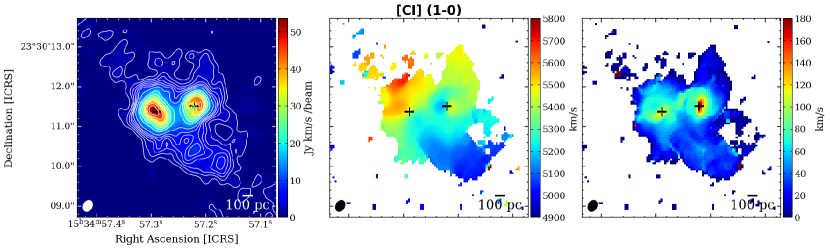
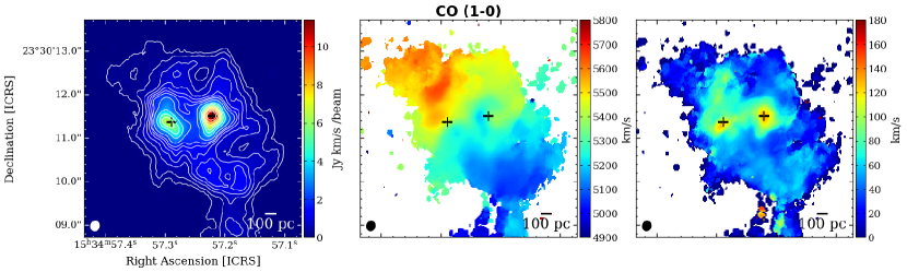
Figure 1: (top) The [C I] (1–0) integrated intensity, velocity field, and velocity dispersion maps of Arp 220. The integrated velocity ranges are 1050 km s^-1 (4845–5895 km s^-1). The contour levels of the integrated intensity map are the peak integrated intensity (54 Jy km s^-1 beam^-1) $\times$ (0.025, 0.050, 0.075, 0.100, 0.125, 0.150, 0.2, 0.3, 0.4, 0.5, 0.6, 0.7, 0.8, 0.9). The plus signs show the nuclei defined by the 880 $\mu$m continuum emission, and the ellipse in the bottom left corner shows the beam size. (bottom) Same as the top figures but for the CO (1–0). The contour levels of the integrated intensity map are the peak integrated intensity (11 Jy km s^-1 beam^-1) $\times$ (0.010, 0.025, 0.050, 0.075, 0.100, 0.125, 0.150, 0.2, 0.3, 0.4, 0.5, 0.6, 0.7, 0.8, 0.9).

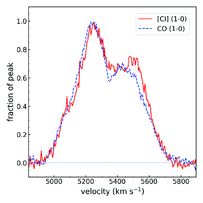
Figure 2: The [C I] (1–0) and CO (1–0) spectra for the central 5region are presented by the solid red and dashed blue lines, respectively. The y-axis is the flux density normalized by the peak.

The integrated intensity, velocity field, and velocity dispersion maps of [C I] (1–0) and CO (1–0) are presented in Figure 1. The integrated intensity maps were created without clipping the intensities. The velocity field and velocity dispersion maps were made after clipping the cleaned image cubes at the 4$\sigma$ level per channel. The apparent distribution of the [C I] (1–0) emission is similar to the CO (1–0) distribution overall. However, the strongest [C I] (1–0) and CO (1–0) peaks are inconsistent, and they are located in the eastern and western nuclei, respectively. An arc-like feature in the [C I] (1–0) map seen around the western nucleus is due to self-absorption. The [C I] (1–0) velocity dispersion is 186 km s^-1 and 117 km s^-1 in the western and eastern nuclei, respectively. On the other hand, the CO (1–0) velocity dispersion is 133 km s^-1 and 128 km s^-1 in the western and eastern nuclei, respectively. Thus, the [C I] (1–0) velocity dispersion is $\sim$1.4 times higher than the CO (1–0) in the western nucleus. In addition, we present the [C I] (1–0) and CO (1–0) spectra for the central 5region (the region with a radius of 25 from the pointing center located between the two nuclei) in Figure 2. The spectral profiles are similar, but subtle differences can be seen at $v$ = 5100–5600 km s^-1.

3.2 Molecular mass

The integrated [C I] (1–0) line flux density within the central 5(1.9 kpc) region is 760 $\pm$ 150 Jy km s^-1. The integrated CO (1–0) line flux density within the same region is 190 $\pm$ 10 Jy km s^-1. Since our data were not corrected with the zero-spacing information and visibilities are clipped, the data suffer from missing flux. For example, we compare the integrated [C I] (1–0) line flux density with the measurement taken by the JCMT (1160 $\pm$ 350 Jy km s^-1 ($\Omega_{\rm PB}$ = 10); Papadopoulos & Greve (2004)). The recovered flux is 66 %. The shortest $uv$ range of our data is 26.9 k$\lambda$, which corresponds to the maximum recoverable scale of 1.75 kpc for Arp 220. Thus, we discuss components smaller than 1.75 kpc in this study. We calculate the line luminosity from the integrated line flux density using Equation (3) of Solomon & Vanden Bout (2005):

$$L^{\prime}_{\rm line}=3.25\times 10^{7}S_{\rm line}\Delta\,v\nu_{\rm obs}^{-2}D_{\rm L}^{2}(1+z)^{-3},$$ (1)

where $L^{\prime}_{\rm line}$ is the luminosity in K km s^-1 pc², $S_{\rm line}\Delta\,v$ is the integrated line flux density in Jy km s^-1, $\nu_{\rm obs}$ is the observing frequency in GHz, $D_{\rm L}$ is the luminosity distance in Mpc, and $z$ is the redshift. The derived line luminosity is summarized in Table Spatially-resolved relation between [C I] ${}^{3}P_{1}$–${}^{3}P_{0}$ and ¹²CO (1–0) in Arp 220. We calculate the [C I] (1–0)/CO (1–0) (hereafter [C I]/CO) luminosity ratio of Arp 220. The derived luminosity ratio is 0.22 $\pm$ 0.04, which is comparable to the average [C I]/CO ratio (0.22 $\pm$ 0.09) of 20 U/LIRGs presented in Valentino et al. (2018).

Assuming the optically thin condition, we calculate the molecular gas mass ($M_{\rm CI}$) from the integrated [C I] (1–0) line flux density using Equation (6) of Bothwell et al. (2017):

$$M_{\rm CI}({\rm H_{2}})=1375.8\frac{D_{\rm L}^{2}}{1+z}\left(\frac{X_{\rm CI}}{10^{-5}}\right)^{-1}\left(\frac{A_{10}}{10^{-7}{\rm s^{-1}}}\right)^{-1}Q_{10}^{-1}S_{\rm CI}\Delta v,$$ (2)

where $M_{\rm CI}$(H₂) is the molecular gas mass in the unit of $M_{\solar}$, $X_{\rm CI}$ is the C I abundance relative to H₂, $A_{10}$ is the Einstein coefficient (= $7.93\times 10^{-8}$ s^-1), $Q_{10}$ is the [C I] excitation factor, and $S_{\rm CI}\Delta v$ is the integrated [C I] (1–0) line flux density. We calculate $M_{\rm CI}$ by applying $X_{\rm CI}$ = $3\times 10^{-5}$, which was used in the previous [C I] (1–0) study of Arp 220 (Papadopoulos & Greve, 2004). We also adopt $Q_{10}$ = 0.48, which is the mean value of $Q_{10}$ for the typical ISM conditions in galaxies where the [C I] lines are globally subthermally excited ($n_{\rm H_{2}}$ = (0.3 – 1.0) $\times$ 10⁴ cm^-3 and $T_{\rm kin}$ = 25 – 80 K) (Papadopoulos et al., 2021). The derived $M_{\rm CI}$ is $(6.0\pm 1.2)\times 10^{9}M_{\solar}$. In addition, we calculate the molecular gas mass ($M_{\rm CO}$) from the integrated CO (1–0) line flux density by using a ULIRG-like CO luminosity-to-H2 mass conversion factor ($\alpha_{\rm CO}$ = 0.8 $M_{\solar}$ pc^-2 (K km s^-1)^-1; Bolatto et al. (2013)) and derive $M_{\rm CO}$ of $(2.4\pm 0.1)\times 10^{9}M_{\solar}$. In this case, $M_{\rm CI}$ is $\sim$2.5 times larger than $M_{\rm CO}$. The relative abundance of CI varies from $1.6\times 10^{-5}$ to $8.4\times 10^{-5}$ depending on the source (e.g., Walter et al. (2011); Valentino et al. (2018); Boogaard et al. (2020)). Jiao et al. (2019) suggest that $X_{\rm CI}$ in local U/LIRGs (Avg. $X_{\rm CI}=(8.3\pm 3.0)\times 10^{-5}$) is about three times higher than $X_{\rm CI}$ of spiral galaxies. When applying this abundance, $M_{\rm CI}$ of Arp 220 results in $(2.2\pm 0.4)\times 10^{9}M_{\solar}$, which is similar to $M_{\rm CO}$. Assuming that $M_{\rm CI}$ is consistent with $M_{\rm CO}$ and the assumed $\alpha_{\rm CO}$ and $Q_{\rm 10}$ are correct, we derive $X_{\rm CI}$ of $7.5\times 10^{-5}$, which is consistent with the average $X_{\rm CI}$ in local U/LILRGs (Jiao et al., 2019) within the errors. Thus, the [C I] (1–0) line can be used as a substitute for CO (1–0) to estimate the molecular gas mass, but we need to carefully choose the parameters, including the relative abundance of C I.

3.3 High-velocity components in the western nucleus

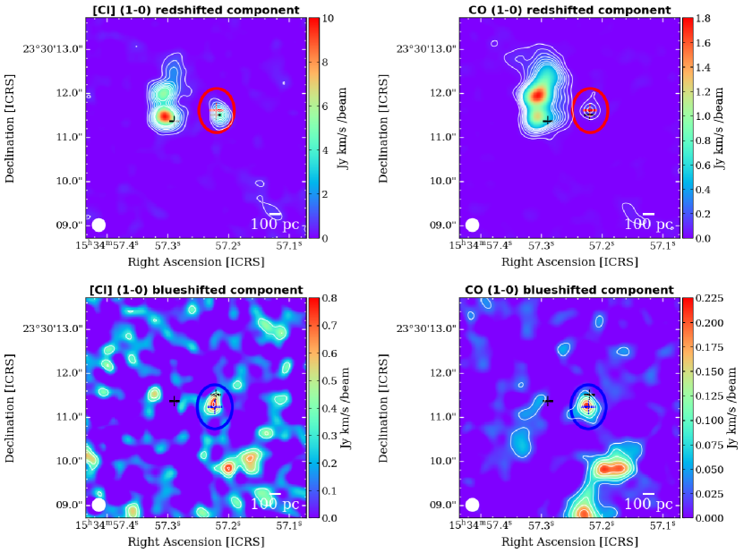
Figure 3: (top) The [C I] (1–0) and CO (1–0) integrated intensity maps of the redshifted component. The integrated velocity range is [5625, 5895] km s^-1 ($\Delta v$ = 270 km s^-1). The contour levels are 0.26 Jy beam^-1 km s^-1 $\times$ (2, 4, 6, 8, 10, 12, 14, 16) for the [C I] map and 25 mJy beam^-1 km s^-1 $\times$ (2, 4, 6, 8, 10, 12, 14, 16) for the CO map. The black plus signs show the nuclei defined by the 880 $\mu$m continuum emission, and the ellipse in the bottom left corner shows the beam size ($\theta$ = 03). The red plus sign shows the peak of the CO redshifted component. We measure the flux densities of the redshifted component (Table Spatially-resolved relation between [C I] ${}^{3}P_{1}$–${}^{3}P_{0}$ and ¹²CO (1–0) in Arp 220) by integrating the pixel values within the red ellipse (08 $\times$ 10). (bottom) Same as the top figures but for the blueshifted component. The integrated velocity range is [4845, 4990] km s^-1 ($\Delta v$ = 140 km s^-1). The contour levels are 0.15 Jy beam^-1 km s^-1 $\times$ (2, 3, 4, 5) for the [C I] map and 18 mJy beam^-1 km s^-1 $\times$ (2, 4, 6, 8, 10) for the CO map. The blue plus sign shows the peak of the CO blueshifted component. We measure the flux densities of the blueshifted component by integrating the pixel values within the blue ellipse (08 $\times$ 10).

Recent high-resolution observations with ALMA discovered the collimated molecular outflow in the western nucleus of Arp 220 (Wheeler et al., 2020; Barcos-Muñoz et al., 2018). The molecular outflow was detected in diffuse and dense gas tracers, such as CO (1–0) and HCN (1–0) lines. We created the CO (1–0) integrated intensity maps of high-velocity components (see Figure 3) by using the same velocity ranges used in Barcos-Muñoz et al. (2018) because it is difficult to identify the morphology of the outflowing components due to the coarse angular resolution. The velocity ranges of the blueshifted and redshifted components are -510 km s^-1 $<v-v_{\rm sys}<$ -370 km s^-1 and 270 km s^-1 $<v-v_{\rm sys}<$ 540 km s^-1, respectively. The systemic velocity is $v_{\rm sys}$ = 5355 $\pm$ 15 km s^-1 for the western nucleus (Sakamoto et al., 1999). As discovered by the previous observations, high-velocity components were detected around the western nucleus (Figure 3). The blueshifted component is located in the south of the western nucleus, whereas the redshifted component is located close to the nucleus. There are also disk components in the maps. In addition, we created the [C I] (1–0) integrated intensity maps using the same velocity ranges (Figure 3). While the blueshifted component around the western nucleus was only marginally detected, the redshifted component was clearly detected. The [C I] (1–0) emission peaks are consistent with the CO (1–0) emission peaks within the beam size. Since the location and velocity of the [C I] (1–0) components are consistent with the CO (1–0), the [C I] (1–0) high-velocity components are likely associated with the outflow. Furthermore, although the angular resolutions are not high enough to reveal the detailed distributions, the redshifted components of [C I] (1–0) and CO (1–0) seem to be slightly separated, implying that the [C I] (1–0) and CO (1–0) distributions are different in the outflow. Future high-resolution observations are necessary to confirm this.

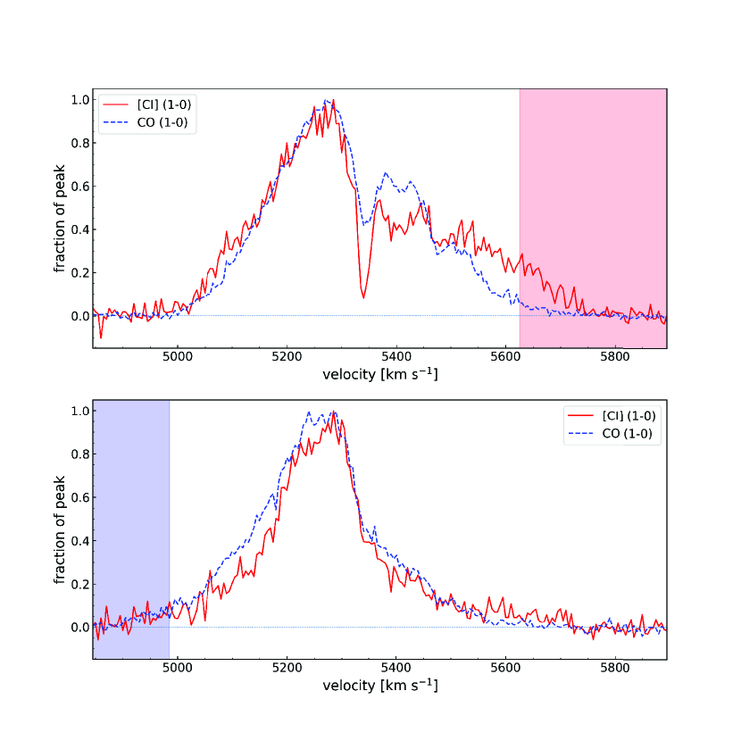
Figure 4: (top) The [C I] (1–0) and CO (1–0) spectra in the peak of the CO redshifted component ([15h34m57.219s, +23D30’11.606”)]; see also the red plus sign in Figure 3 (top)). The y-axis is the flux density normalized by the peak. The red background color shows the velocity range of the redshifted component. (bottom) The spectra in the peak of the CO blueshifted component ([15h34m57.222s, +23D30’11.231”]; see also the blue plus sign in Figure 3 (bottom)). The blue background color shows the velocity range of the blueshifted component.

We calculate the molecular gas mass of the high-velocity components from the integrated [C I] (1–0) and CO (1–0) line flux densities in the same way as the previous section. Firstly, we measure the line flux densities within 08 $\times$ 10 from the CO (1–0) peak of each high-velocity component. The regions are shown by the blue and red ellipses in Figure 3 and are chosen to include the lowest (2$\sigma$) contour. The image RMS was measured in the line-free region of each integrated intensity map. Then, we calculate $M_{\rm CI}$ by applying $Q_{10}$ = 0.47 (Papadopoulos & Greve, 2004) and $X_{\rm CI}=7.5\times 10^{-5}$ we derive in §3.2 and $M_{\rm CO}$ by using $\alpha_{\rm CO}$ = 0.8 $M_{\solar}$ pc^-2 (K km s^-1)^-1 (Bolatto et al., 2013). The derived molecular gas mass is presented in Table Spatially-resolved relation between [C I] ${}^{3}P_{1}$–${}^{3}P_{0}$ and ¹²CO (1–0) in Arp 220. While $M_{\rm CI}$ of the blueshifted component is 0.76 times smaller than $M_{\rm CO}$, $M_{\rm CI}$ of the redshifted component is 5.3 times larger than $M_{\rm CO}$. One possibility is that $M_{\rm CI}$ of the redshifted component is overestimated due to the contamination of gas associated with the main body. The spectral profiles of the redshifted component are significantly different between [C I] (1–0) and CO (1–0) (Figure 4), implying that the [C I] (1–0) and CO (1–0) emission traces different components. However, even if we take into account this possibility, it is not possible to explain the difference between $M_{\rm CI}$ and $M_{\rm CO}$ of the blueshifted component. These inconsistencies indicate that the parameters, such as $\alpha_{\rm CO}$, $X_{\rm CI}$ and $Q_{10}$, differ between the galaxy-averaged and outflow components and even between the blueshifted and redshifted components. For example, matching $M_{\rm CO}$ of the redshifted component with $M_{\rm CI}$ requires a CO luminosity-to-H₂ conversion factor of $\alpha_{\rm CO}$ = 4.3. This value is larger than the ULIRG-like CO luminosity-to-H2 mass conversion factor but similar to the standard CO luminosity-to-H2 mass conversion factor (e.g., $\alpha_{\rm CO}$ = 4.35 $M_{\solar}$ pc^-2 (K km s^-1)^-1 Bolatto et al. (2013)). Future high-resolution [C I] observations would reveal the detailed morphology of the atomic carbon outflow, allowing us to derive the spatial distribution of the different physical parameters.

4 Discussion

4.1 The relation between [C I] and CO

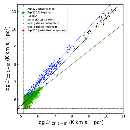
Figure 5: Plot of the [C I] (1–0) luminosity vs. the CO (1–0) luminosity. The different symbols present the different samples. The green dots are star forming environments in Arp 220. The blue circles are resolved galaxies in the local universe (Jiao et al., 2019). The other symbols show the integrated values. The green star and red circle are the values integrated over the central 5region and redshifted component of Arp 220, respectively. The black triangles are U/LIRGs (Liu et al. (2015); Kamenetzky et al. (2016); Valentino et al. (2018)), the yellow triangles are proto-cluster galaxies at $z$ = 2,2 (Emonts et al., 2018), and the blue triangles are integrated values of local galaxies (Jiao et al., 2019).

We plot the [C I] (1-0) and CO (1–0) luminosities of Arp 220 and the literature samples of local galaxies (non-U/LIRGs) (Jiao et al., 2019), unresolved U/LIRGs (Liu et al. (2015); Kamenetzky et al. (2016); Valentino et al. (2018)), and proto-cluster galaxies at $z$ = 2.2 (Emonts et al., 2018) in Figure 5. Jiao et al. (2019) found two different linear relations in the [C I] (1–0) vs. CO (1–0) plot. One is for the non-U/LIRGs, and the other is for the U/LIRGs and the proto-cluster galaxies. The best-fit lines for these two groups are shown by dashed blue and black lines in Figure 5. Arp 220 (integrated) is consistent with the linear relation for the unresolved ULIRG sample.

We check whether the [C I] (1–0) luminosity correlates with the CO (1–0) luminosity at $\sim$100 pc scale using the channel maps of Arp 220. We create beam-matched maps by smoothing the original channel maps and perform the pixel binning. The final angular resolution is 03, which corresponds to $\sim$110 pc. The pixel size is 57 pc $\times$ 57 pc, and the velocity resolution is 5 km s^-1. Then, we measure the [C I] (1–0) and CO (1–0) luminosities per pixel, but we exclude pixels in which either [C I] (1–0) or CO (1–0) flux densities are below the 3$\sigma$ level. The lower limits of the [C I] (1–0) and CO (1–0) luminosities are $1.5\times 10^{5}$ K km s^-1 pc² and $3.0\times 10^{5}$ K km s^-1 pc², respectively. We also exclude pixels within 300 pc from each nucleus because self-absorption can affect our interpretation.

We plot the [C I] (1–0) and CO (1–0) luminosities measured in each pixel (Arp 220 (channel map)) in Figure 5 and perform a linear fitting to the [C I] (1–0) and CO (1–0) data points using the python package linmix (Kelly, 2007). This gives the best-fit line,

$$\log L^{\prime}_{\rm CO(1-0)}=(0.76\pm 0.01)\log L^{\prime}_{\rm[CI](1-0)}+(1.89\pm 0.05),$$ (3)

but we exclude pixels in which the [C I] (1–0) luminosity is below log $L^{\prime}_{\rm[CI](1-0)}$ = 5.3 for fitting because the sampled data are dominated by noise. The slope of the best-fit line is smaller than the unity. Such a sublinear relation between $L^{\prime}_{\rm[CI](1-0)}$ and $L^{\prime}_{\rm CO(1-0)}$ has been found in the previous study on a ULIRG, IRAS F18293-3413 (Saito et al., 2020). While the [C I] (1–0) and CO (1–0) luminosities integrated across the system of Arp 220 follow the empirical linear relation for the unresolved ULIRG sample, we find a sublinear relation between $L^{\prime}_{\rm[CI](1-0)}$ and $L^{\prime}_{\rm CO(1-0)}$ using the spatially-resolved data of Arp 220, indicating that the [C I]/CO luminosity ratios are not constant in the system.

4.2 Variations in the C I/CO abundance ratios

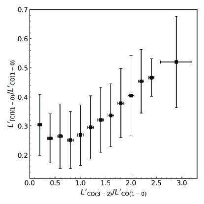
Figure 6: Plot of the average [C I] (1–0)/CO (1–0) luminosity ratio vs. the CO (3–2)/CO (1–0) luminosity ratio.

We check the dependence of the [C I]/CO luminosity ratio on the CO (3–2)/CO (1–0) ratio ($R_{\rm CO}$) in order to investigate what causes variations of $L^{\prime}_{\rm[CI](1-0)}$/$L^{\prime}_{\rm CO(1-0)}$ in Arp 220. In general, $R_{\rm CO}$ is enhanced in active star forming regions because increasing the gas density and heating the interstellar medium due to ultraviolet (UV) emission from newly born stars are responsible for collisionally exciting the CO gas to the $J$ = 3 level. Thus, $R_{\rm CO}$ can be interpreted as an indicator of the physical properties of the gas. We divide the pixels into bins with $\Delta R_{\rm CO}$ = 0.2 (0.1 $\leq R_{\rm co}<$ 2.5) and the others ($R_{\rm co}\geq 2.5$) because the sample size is small in a range of $R_{\rm co}\geq 2.5$. Then, we calculate the average $L^{\prime}_{\rm[CI](1-0)}/L^{\prime}_{\rm CO(1-0)}$ of each bin and plot them as a function of $R_{\rm CO}$ in Figure 6. As a result, the average $L^{\prime}_{\rm[CI](1-0)}/L^{\prime}_{\rm CO(1-0)}$ is roughly constant up to $R_{\rm CO}$ = 1.0 and then increases with $R_{\rm CO}$.

We perform non-local thermodynamic equilibrium (non-LTE) analysis using the radiative transfer code RADEX (van der Tak et al., 2007) to check whether this trend can be reproduced by changing the physical properties of gas. RADEX has been developed to infer the physical and chemical parameters, such as temperature, density, and molecular abundances, in molecular clouds. It requires the line width that reflects the internal velocity dispersions of molecular clouds as one of the input parameters. However, we cannot measure the line width using our maps due to coarse angular resolutions. We thus adopt the typical line-width of molecular clouds in the Galaxy (5 km s^-1; e.g., Heyer et al. (2009)), assuming that similar molecular clouds form in Arp 220. We fixed the CO column density ($N_{\rm CO}$) to 5 $\times$ 10¹⁷ cm^-2 based on the radiative transfer analysis (Sliwa & Downes, 2017). They performed RADEX calculations to model the CO lines of Arp 220 and derived the mean $N_{\rm co}$ of (1.1–2.3) $\times 10^{19}$ cm^-2 (d$V$ = 120–320 km s^-1). This gives $N_{\rm co}$/d$V$ of (7–9) $\times$ 10¹⁶. We thus adopt $N_{\rm CO}$ of $5\times 10^{17}$ (d$V$ = 5 km s^-1). We also fix the background temperature to 2.73 K. We vary the C I column density ($N_{\rm CI}$) and the kinetic temperature ($T_{\rm k}$) or the H₂ density ($n_{\rm H_{2}}$), and calculate the radiation temperature of the lines. RADEX yields the opacity of [C I] (1–0) $<$1 and the opacity of CO (3–2) $>$1 for most conditions. The opacity of CO (1–0) is large ($>$1) at the low $T_{\rm kin}$ and $n_{H_{2}}$ and decreases with increasing $T_{\rm kin}$ and $n_{\rm H_{2}}$. The CO (1–0) is optically thin in regions with $R_{\rm CO}>1$.

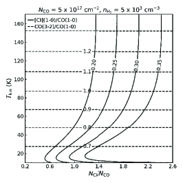
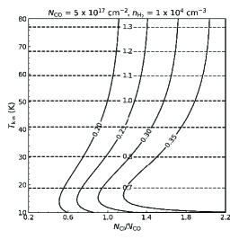
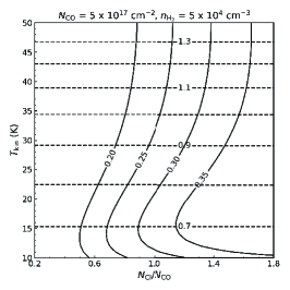
Figure 7: Results of RADEX calculation when the H₂ density is fixed to $n_{\rm H_{2}}$ = [0.5, 1.0, 5.0] $\times$ 10⁴ cm^-3 and the CO column density is fixed to $N_{\rm CO}$ = 5 $\times$ 10¹⁷ cm^-2. The solid black lines show the constant [C I] (1–0)/CO (1–0) line ratios, and the dashed black lines show the constant CO (3–2)/CO (1–0) line ratios.

In Figure 7, we show the results of RADEX calculation when the H₂ density is fixed to $n_{\rm H_{2}}$ = [0.5, 1.0, 5.0] $\times$ 10⁴ cm^-3. These fixed densities are similar to or higher than the mean gas densities derived by Sliwa & Downes (2017). Their radiative transfer analysis yields the mean gas densities of 10^2.54–10^3.76 cm^-3 and the mean kinetic temperatures of 105–240 K. Relatively high densities ($\geq 5\times 10^{4}$ cm^-3) are required for reproducing high CO (3-2)/CO (1-0) line ratios at the kinetic temperatures of $<$ 300 K. In addition, Israel et al. (2015) found that the interstellar medium in LIRGs is dominated by dense ($n_{\rm H2}$ = 10⁴–10⁵ cm^-3) and moderately warm ($T_{\rm kin}\sim$ 30 K) gas clouds. Considering these results, the density range adopted for our RADEX calculations is likely appropriate for typical gas conditions in IR-bright galaxies, including Arp 220.

The [C I]/CO line ratio decreases with increasing $R_{\rm CO}$ (or $T_{\rm kin}$) at the fixed C I/CO abundance ratio, except under kinetic temperature below 10 K. For example, in the case where $n_{\rm H_{2}}=1\times 10^{4}$ cm^-3 and $N_{\rm CI}$/$N_{\rm CO}$ = 1.0 (Figure 7 (middle)), the [C I]/CO line ratio is $\sim$0.26 at $R_{\rm CO}$ = 0.8 and decreases to $\sim$0.19 at $R_{\rm CO}$ = 1.2. This is different from the observed trend (Figure 6). We also check the modeled line ratios when the kinetic temperature is fixed to $T_{\rm k}$ = [75, 100, 125] K and the H₂ density is changed. In this case, the [C I]/CO line ratio does not change significantly with increasing $R_{\rm CO}$ (or $n_{\rm H_{2}}$) at the fixed C I/CO abundance ratio. According to our RADEX calculation, the observed trend is not fully explained by changing only the temperature or gas density.

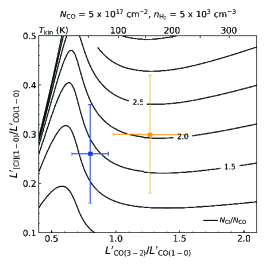
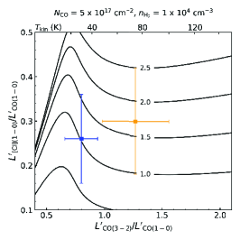
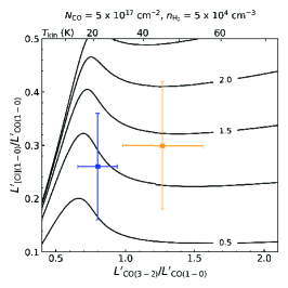
Figure 8: Plot of the [C I] (1–0)/CO (1–0) luminosity ratio vs. the CO (3–2)/CO (1–0) luminosity ratio for comparison between the observed and modeled data. The orange and blue squares show the representative parameters of Group 1 (CO (3–2)/CO(1–0) $\geq$ 1) and Group 2 (CO (3–2)/CO (1–0) $<$ 1), respectively. These parameters are calculated from the observations. The black lines show the constant C I/CO abundance ratios calculated from the RADEX analysis when the H₂ density is fixed to $n_{\rm H_{2}}$ = [0.5, 1.0, 5.0] $\times$ 10⁴ cm^-3 and the CO column density is fixed to $N_{\rm CO}$ = 5 $\times$ 10¹⁷ cm^-2.

Furthermore, we compare the RADEX results with the observational data. For simplicity, we divide the observational data points (pixels) into two groups by $R_{\rm CO}$. Group 1 has $R_{\rm CO}\geq 1$, and Group 2 has $R_{\rm CO}<1$. Then we compute the mean $L^{\prime}_{\rm[CI](1-0)}/L^{\prime}_{\rm CO(1-0)}$ and $R_{\rm CO}$ of each group. Group 1 has $L^{\prime}_{\rm[CI](1-0)}/L^{\prime}_{\rm CO(1-0)}$ = 0.30 $\pm$ 0.12 and $R_{\rm CO}$ = 1.27 $\pm$ 0.29, and Group 2 has $L^{\prime}_{\rm[CI](1-0)}/L^{\prime}_{\rm CO(1-0)}$ = 0.26 $\pm$ 0.10 and $R_{\rm CO}$ = 0.80 $\pm$ 0.14. In Figure 8, we show the parameter sets ( $L^{\prime}_{\rm[CI](1-0)}/L^{\prime}_{\rm CO(1-0)}$ and $R_{\rm CO}$) of Group 1 and Group 2 by the orange and blue squares, respectively, and plot lines to show the constant C I/CO abundance ratios calculated from the RADEX analysis when the H₂ density is fixed to $n_{\rm H_{2}}$ = [0.5, 1.0, 5.0] $\times$ 10⁴ cm^-3. We find that the C I/CO abundance ratio at Group 1 is similar to or a few times higher than that at Group 2. For example, in the case of $n_{\rm H_{2}}=1\times 10^{4}$ cm^-3 (Figure 8 (middle)), the C I/CO abundance ranges from 0.69 to 2.00 for Group 1, and it ranges from 0.18 to 1.32 for Group 2. While the C I/CO abundance ranges partially overlap between the two groups, an elevated abundance ratio is likely to be required to explain the observed high $L^{\prime}_{\rm[CI](1-0)}/L^{\prime}_{\rm CO(1-0)}$ in regions with high $R_{\rm CO}$. We obtain similar results when calculating the abundance ratio by changing the $H_{2}$ density. The study of the central region of the starburst galaxy NGC 1808 reaches a similar conclusion that $L^{\prime}_{\rm[CI](1-0)}/L^{\prime}_{\rm CO(1-0)}$ is enhanced owing to high excitation and atomic carbon abundance (Salak et al., 2019). We also check the RADEX results when the parameters ($N_{\rm co}$ or d$V$) are fixed to different values. For example, we adopt $N_{\rm CO}$ = [0.1, 0.5, 1.0] $\times 10^{18}$ cm^-2. While the C I/CO abundance ratios for Group 1 are on average higher than those for Group 2 in all three cases, the difference between Group 1 and Group 2 decreases with decreasing $N_{\rm CO}$. The same trend is seen when d$V$ is increased, which is a natural consequence of the RADEX calculation as it depends on $N_{\rm co}$/d$V$. In this study, assuming a constant $N_{\rm CO}$, we have performed the radiative transfer analysis. If $N_{\rm CO}$ is significantly changing from one region to another in the science target, the cause of various $L^{\prime}_{\rm[CI](1-0)}$/$L^{\prime}_{\rm CO(1-0)}$ cannot be straightforward to interpret. Under the assumption that $N_{\rm CO}$ is constant in the observed region, the comparison between the observational and modeled data suggests that the C I/CO abundance ratio varies at $\sim$100 pc scale in Arp 220.

4.3 High line ratio in the redshifted component

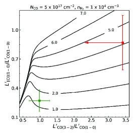
Figure 9: The same as Figure 8, but the symbols are different. The red and green squares show the average line ratios for the redshifted component and the main body of Arp 220, respectively. The black lines show the constant C I/CO abundance ratios calculated from the RADEX analysis when the CO column density is fixed to $N_{\rm CO}$ = 5 $\times$ 10¹⁷ cm^-2 and the H₂ density is fixed to $n_{\rm H_{2}}$ = 1.0 $\times$ 10⁴ cm^-3.

We calculate the [C I]/CO luminosity ratios of the high-velocity components using pixels in which both [C I] (1–0) and CO (1–0) flux densities are above the 3$\sigma$ levels. The average $L^{\prime}_{\rm[CI](1-0)}/L^{\prime}_{\rm CO(1-0)}$ of the redshifted component is 0.87 $\pm$ 0.28, which is four times higher than the average $L^{\prime}_{\rm[CI](1-0)}/L^{\prime}_{\rm CO(1-0)}$ of Arp 220 (0.22 $\pm$ 0.04) (see Figure 5). The average $L^{\prime}_{\rm[CI](1-0)}/L^{\prime}_{\rm CO(1-0)}$ of the blueshifted component is 0.41 $\pm$ 0.11, but only five pixels meet the threshold. High [C I]/CO line ratios have been found in the root point of the bipolar outflow of the NGC 253 ($\sim$0.4–0.6; Krips et al. (2016)) and the bipolar outflow of the Galactic molecular cloud G5.2-0.74N ($\sim$0.4; Little et al. (1998)). While we cannot rule out the possibility that the [C I] (1–0) and CO (1–0) emission traces different components, as mentioned in §3.3, we suggest that the high [C I]/CO line ratios are caused by an elevated C I/CO abundance ratio based on our RADEX analysis (Figure 9). Since the CO (3–2) spectra of the redshifted component are affected by contamination from other molecular lines, possibly H¹³CN (4–3), we calculate an upper limit for $R_{\rm CO}$ in the redshifted component and plot it with $L^{\prime}_{\rm[CI](1-0)}/L^{\prime}_{\rm CO(1-0)}$ of the redshifted component in Figure 9. The high C I/CO abundance ratio is required for the [C I]/CO luminosity ratios measured in the redshifted component, regardless of the value of $R_{\rm CO}$.

The possibility of CO-poor/C I-rich molecular gas in outflows is predicted by the theoretical study (Papadopoulos et al., 2018). Low-density, gravitationally-unbound molecular gas is expected to be in outflows because of Kelvin-Helmholtz instabilities and shear acting on the envelopes of denser clouds. Such a gas phase could be invisible in CO due to the destruction of CO induced by the CRs, which have been identified as a potentially more effective agent of CO-destruction than far-UV photons (e.g., Bialy & Sternberg (2015); Bisbas et al. (2015); Papadopoulos et al. (2018)). Varenius et al. (2016) found an elongated feature extending 09 from the western nucleus in the radio continuum maps at 150 MHz, 1.4 GHz, and 6 GHz, indicating the presence of outflow. This elongated feature requires the shock-acceleration of CRs in the outflow. In addition, the $\gamma$-ray observations suggest the presence of an AGN, providing the extra CRs, in the western nucleus (Yoast-Hull et al., 2017). In the high-velocity components of Arp 220, CRs could help enrich C I by destroying CO.

Another possibility of the high $L^{\prime}_{\rm[CI](1-0)}/L^{\prime}_{\rm CO(1-0)}$ is the CO dissociation by mechanical perturbation such as shocks and the strong radiation field. The dissociation of C-bearing molecules such as CO can significantly enhance the C abundance in active environments where shocks occur and/or strong UV and X-ray radiation fields associated with intense star formation and an AGN (e.g., Meijerink et al. (2007), Meijerink et al. (2011), Tanaka et al. (2011)). Krips et al. (2016) found that the [C I] (1–0) line emission is enhanced compared to CO (1–0) in the region of NGC 253 where outflows or shocks are important dynamical players, suggesting that shocks affect the [C I]/CO ratio.

5 Summary

We present the new [C I] (1–0) map of Arp 220 and the uv-matched CO (1–0) map as well. The distributions and kinematics of the [C I] (1–0) and CO (1–0) emission are similar overall, but the [C I] (1–0) velocity dispersion is 1.4 times higher than the CO (1–0) in the western nucleus.

The [C I]/CO luminosity ratio integrated over the system is 0.22 $\pm$ 0.04, which is comparable to the previous measurements of 20 U/LIRGs, and the [C I] (1–0) and CO (1–0) luminosities of Arp 220 are consistent with the empirical linear relation between $L^{\prime}_{\rm[CI](1-0)}$ and $L^{\prime}_{\rm CO(1-0)}$ for the unresolved ULIRG sample. However, when measuring the [C I] (1–0) and CO (1–0) luminosities per pixel (1 pix = 57 pc $\times$ 57 pc, $\Delta v$ = 5 km s^-1), we find a sublinear relation between them, indicating that the [C I]/CO luminosity ratios are not constant in Arp 220.

We investigate the dependence of the [C I]/CO luminosity ratio on $R_{\rm CO}$. The average $L^{\prime}_{\rm[CI](1-0)}/L^{\prime}_{\rm CO(1-0)}$ is almost constant up to $R_{\rm CO}$ = 1.0 and then increases with $R_{\rm CO}$. We perform non-LTE analysis using the radiative transfer code RADEX to check whether this trend can be reproduced by changing the physical properties of the gas or the abundance ratio. As a result, a high abundance ratio is required to explain the enhanced $L^{\prime}_{\rm[CI](1-0)}/L^{\prime}_{\rm CO(1-0)}$ in regions with $R_{\rm CO}>1$. This suggests that the C I/CO abundance ratio varies at $\sim$100 pc scale within the system of Arp 220.

Finally, the atomic carbon was detected in the high-velocity components, which are likely to be the outflow. The average $L^{\prime}_{\rm[CI](1-0)}/L^{\prime}_{\rm CO(1-0)}$ of the redshifted component is 0.87 $\pm$ 0.28, which is four times higher than the average $L^{\prime}_{\rm[CI](1-0)}/L^{\prime}_{\rm CO(1-0)}$ of Arp 220. The theoretical work on the CR-driven astrochemistry supports such a gas phase of C I-rich and CO-poor. CRs could help enrich CI by destroying CO in the outflowing gas.

We thank Qian Jiao for providing the data of local galaxies published in Jiao et al. (2019). We also thank Kouichiro Nakanishi for advising us about the data reduction. J.U. was supported by the ALMA Japan Research Grant of NAOJ ALMA Project, NAOJ-ALMA-258. D.I. is supported by JSPS KAKENHI Grant Number JP18H03725.

This paper makes use of the following ALMA data: ADS/JAO.ALMA#2013.1.00368.S, ADS/JAO.ALMA#2015.1.00113.S, ADS/JAO.ALMA#2017.1.00042.S. ALMA is a partnership of ESO (representing its member states), NSF (USA) and NINS (Japan), together with NRC (Canada), MOST and ASIAA (Taiwan), and KASI (Republic of Korea), in cooperation with the Republic of Chile. The Joint ALMA Observatory is operated by ESO, AUI/NRAO and NAOJ.

Data analysis was carried out on the Multi-wavelength Data Analysis System operated by the Astronomy Data Center (ADC), National Astronomical Observatory of Japan.

The [C I] and CO measurements in the central 5region of Arp 220 $S_{\rm[CI]}\Delta v$ 760 $\pm$ 150 Jy km s^-1 $S_{\rm CO}\Delta v$ 190 $\pm$ 10 Jy km s^-1 $L^{\prime}_{\rm[CI]}$ (6.6 $\pm$ 1.3) $\times$ 10⁸ K km s^-1 pc^-2 $L^{\prime}_{\rm CO}$ (3.0 $\pm$ 0.2) $\times$ 10⁹ K km s^-1 pc^-2 $L^{\prime}_{\rm[CI]}/L^{{}^{\prime}}_{\rm CO}$ 0.22 $\pm$ 0.04

The [C I] and CO measurements of the high-velocity components Component $S_{\rm[CI]}\Delta v$ $S_{\rm CO}\Delta v$ $M_{\rm CI}$ $M_{\rm CO}$ $M_{\rm CI}$/$M_{\rm CO}$ (Jy km s^-1) (Jy km s^-1) ($M_{\solar}$) ($M_{\solar}$) Redshifted component 5.3 $\pm$ 1.1 0.25 $\pm$ 0.03 $(1.7\pm 0.4)\times 10^{7}$ $(3.2\pm 0.4)\times 10^{6}$ 5.3 $\pm$ 1.3 Blueshifted component 1.0 $\pm$ 0.2 0.33 $\pm$ 0.03 $(3.2\pm 0.6)\times 10^{6}$ $(4.2\pm 0.4)\times 10^{6}$ 0.76 $\pm$ 0.17 Columns 2 and 3: The integrated [C I] (1–0) and CO (1–0) line flux density measured within $0\farcs 8\times 1\farcs 0$ from the CO (1–0) peak of each high-velocity component. Columns 4 and 5: The molecular gas mass estimated from the [C I] (1–0) and CO (1–0) line flux density by applying $X_{\rm CI}=7.5\times 10^{-5}$ and $\alpha_{\rm CO}$ = 0.8 $M_{\solar}$ pc^-2 (K km s^-1)^-1.

Channel maps of the [C I] (1–0)/CO (1–0) luminosity ratio

We present a figure with channel maps of the [C I]/CO luminosity. We rebinned three channels to reduce the number of channels for plotting. The final velocity resolution is 15 km s^-1.

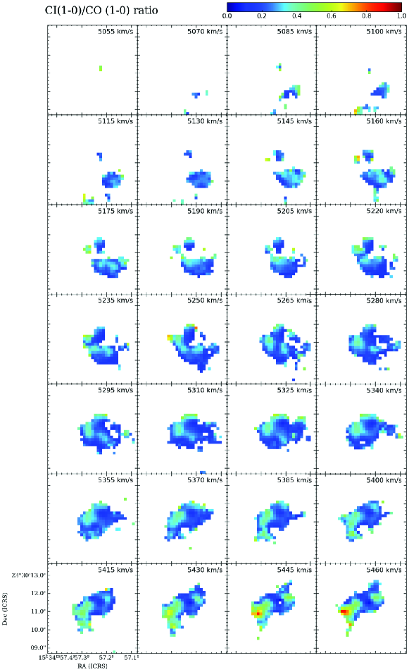
Figure 10: Channel maps of the [C I] (1–0)/CO (1–0) luminosity ratio. The velocity resolution is 15 km s^-1.

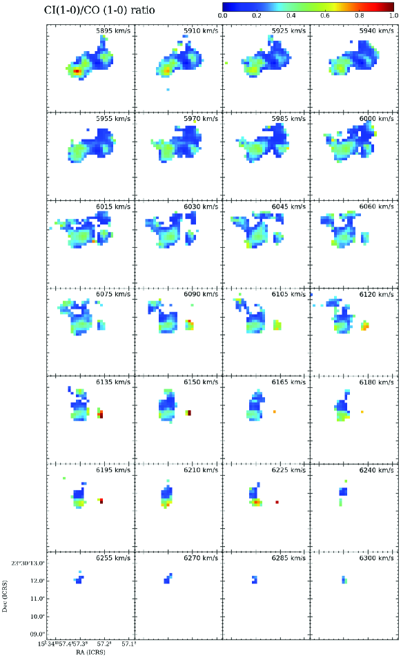
Figure 10: Continued.

References

- Andreani (2015) Andreani, P. 2015, ALMA Cycle 3 Proposer’s Guide and Capabilities, Version 1.0, ALMA. https://almascience.nao.ac.jp/documents-and-tools/cycle3/alma-proposers-guide
- Andreani (2017) Andreani, P. 2017, ALMA Cycle 5 Proposer’s Guide and Capabilities, Version 1.0, ALMA. https://almascience.nao.ac.jp/documents-and-tools/cycle5/alma-proposers-guide
- Armus et al. (2007) Armus, L., Charmandaris, V., Bernard-Salas, J., et al. 2007, ApJ, 656, 148
- Armus et al. (2009) Armus, L., Mazzarella, J. M., Evans, A. S., et al. 2009, PASP, 121, 559
- Barcos-Muñoz et al. (2018) Barcos-Muñoz, L., Aalto, S., Thompson, T. A., et al. 2018, ApJ, 853, L28
- Bialy & Sternberg (2015) Bialy, S. & Sternberg, A. 2015, MNRAS, 450, 4424
- Bisbas et al. (2015) Bisbas, T. G., Papadopoulos, P. P., & Viti, S. 2015, ApJ, 803, 37
- Bolatto et al. (2013) Bolatto, A. D., Wolfire, M., & Leroy, A. K. 2013, ARA&A, 51, 207
- Boogaard et al. (2020) Boogaard, L. A., van der Werf, P., Weiss, A., et al. 2020, ApJ, 902, 109
- Bothwell et al. (2017) Bothwell, M. S., Aguirre, J. E., Aravena, M., et al. 2017, MNRAS, 466, 2825
- Emonts et al. (2018) Emonts, B. H. C., Lehnert, M. D., Dannerbauer, H., et al. 2018, MNRAS, 477, L60
- Genzel et al. (1998) Genzel, R., Lutz, D., Sturm, E., et al. 1998, ApJ, 498, 579
- Greve et al. (2009) Greve, T. R., Papadopoulos, P. P., Gao, Y., et al. 2009, ApJ, 692, 1432
- Heyer et al. (2009) Heyer, M., Krawczyk, C., Duval, J., et al. 2009, ApJ, 699, 1092
- Israel et al. (2015) Israel, F. P., Rosenberg, M. J. F., & van der Werf, P. 2015, A&A, 578, A95
- Jiao et al. (2017) Jiao, Q., Zhao, Y., Zhu, M., et al. 2017, ApJ, 840, L18
- Jiao et al. (2019) Jiao, Q., Zhao, Y., Lu, N., et al. 2019, ApJ, 880, 133
- Kamenetzky et al. (2016) Kamenetzky, J., Rangwala, N., Glenn, J., et al. 2016, ApJ, 829, 93
- Kelly (2007) Kelly, B. C. 2007, ApJ, 665, 1489
- Kennicutt (1998) Kennicutt, R. C. 1998, ApJ, 498, 541
- Krips et al. (2016) Krips, M., Martín, S., Sakamoto, K., et al. 2016, A&A, 592, L3
- Little et al. (1998) Little, L. T., Kelly, M. L., & Murphy, B. T. 1998, MNRAS, 294, 105
- Liu et al. (2015) Liu, D., Gao, Y., Isaak, K., et al. 2015, ApJ, 810, L14
- Lundgren (2013) Lundgren, A. 2013, ALMA Cycle 2 Technical Handbook Version 1.1, ALMA. https://almascience.nao.ac.jp/documents-and-tools/cycle-2/alma-technical-handbook
- Meijerink et al. (2007) Meijerink, R., Spaans, M., & Israel, F. P. 2007, A&A, 461, 793
- Meijerink et al. (2011) Meijerink, R., Spaans, M., Loenen, A. F., et al. 2011, A&A, 525, A119
- McMullin et al. (2007) McMullin, J. P., Waters, B., Schiebel, D., et al. 2007, \asp, 376, 127
- Michiyama et al. (2021) Michiyama, T., Saito, T., Tadaki, K.-. ichi ., et al. 2021, arXiv:2107.12529
- Miyamoto et al. (2021) Miyamoto, Y., Yasuda, A., Watanabe, Y., et al. 2021, PASJ, 73, 552
- Norris (1988) Norris, R. P. 1988, MNRAS, 230, 345
- Papadopoulos et al. (2018) Papadopoulos, P. P., Bisbas, T. G., & Zhang, Z.-Y. 2018, MNRAS, 478, 1716
- Papadopoulos & Greve (2004) Papadopoulos, P. P. & Greve, T. R. 2004, ApJ, 615, L29
- Papadopoulos et al. (2004) Papadopoulos, P. P., Thi, W.-F., & Viti, S. 2004, MNRAS, 351, 147
- Papadopoulos et al. (2021) Papadopoulos, P., Dunne, L., & Maddox, S. 2021, arXiv:2111.02260
- Planck Collaboration et al. (2016) Planck Collaboration, Ade, P. A. R., Aghanim, N., et al. 2016, A&A, 594, A13
- Rangwala et al. (2011) Rangwala, N., Maloney, P. R., Glenn, J., et al. 2011, ApJ, 743, 94
- Saintonge et al. (2017) Saintonge, A., Catinella, B., Tacconi, L. J., et al. 2017, ApJS, 233, 22
- Saito et al. (2020) Saito, T., Michiyama, T., Liu, D., et al. 2020, MNRAS, 497, 3591
- Sakamoto et al. (1999) Sakamoto, K., Scoville, N. Z., Yun, M. S., et al. 1999, ApJ, 514, 68
- Sakamoto et al. (2008) Sakamoto, K., Wang, J., Wiedner, M. C., et al. 2008, ApJ, 684, 957
- Salak et al. (2019) Salak, D., Nakai, N., Seta, M., et al. 2019, ApJ, 887, 143
- Scoville et al. (2017) Scoville, N., Murchikova, L., Walter, F., et al. 2017, ApJ, 836, 66
- Sliwa & Downes (2017) Sliwa, K. & Downes, D. 2017, A&A, 604, A2
- Solomon & Vanden Bout (2005) Solomon, P. M. & Vanden Bout, P. A. 2005, ARA&A, 43, 677
- Tanaka et al. (2011) Tanaka, K., Oka, T., Matsumura, S., et al. 2011, ApJ, 743, L39
- Teng et al. (2015) Teng, S. H., Rigby, J. R., Stern, D., et al. 2015, ApJ, 814, 56
- Valentino et al. (2018) Valentino, F., Magdis, G. E., Daddi, E., et al. 2018, ApJ, 869, 27
- van der Tak et al. (2007) van der Tak, F. F. S., Black, J. H., Schöier, F. L., et al. 2007, A&A, 468, 627
- Varenius et al. (2016) Varenius, E., Conway, J. E., Martí-Vidal, I., et al. 2016, A&A, 593, A86
- Walter et al. (2011) Walter, F., Weiß, A., Downes, D., et al. 2011, ApJ, 730, 18
- Wheeler et al. (2020) Wheeler, J., Glenn, J., Rangwala, N., et al. 2020, ApJ, 896, 43
- Yoast-Hull et al. (2017) Yoast-Hull, T. M., Gallagher, J. S., Aalto, S., et al. 2017, MNRAS, 469, L89
The [C \emissiontypeI] and CO measurements in the central 5\arcsecregion of Arp 220 760 150 Jy km s-1 190 10 Jy km s-1 (6.6 1.3) 108 K km s-1 pc-2 (3.0 0.2) 109 K km s-1 pc-2 0.22 0.04
The [C \emissiontypeI] and CO measurements of the high-velocity components Component / (Jy km s-1) (Jy km s-1) () () Redshifted component 5.3 1.1 0.25 0.03 5.3 1.3 Blueshifted component 1.0 0.2 0.33 0.03 0.76 0.17 {tabnote} Columns 2 and 3: The integrated [C \emissiontypeI] (1–0) and CO (1–0) line flux density measured within from the CO (1–0) peak of each high-velocity component. Columns 4 and 5: The molecular gas mass estimated from the [C \emissiontypeI] (1–0) and CO (1–0) line flux density by applying and = 0.8 pc-2 (K km s-1)-1.
Channel maps of the [C \emissiontypeI] (1–0)/CO (1–0) luminosity ratio