Poseur: Direct Human Pose Regression with Transformers

Abstract

We propose a direct, regression-based approach to 2D human pose estimation from single images. We formulate the problem as a sequence prediction task, which we solve using a Transformer network. This network directly learns a regression mapping from images to the keypoint coordinates, without resorting to intermediate representations such as heatmaps. This approach avoids much of the complexity associated with heatmap-based approaches. To overcome the feature misalignment issues of previous regression-based methods, we propose an attention mechanism that adaptively attends to the features that are most relevant to the target keypoints, considerably improving the accuracy. Importantly, our framework is end-to-end differentiable, and naturally learns to exploit the dependencies between keypoints. Experiments on MS-COCO and MPII, two predominant pose-estimation datasets, demonstrate that our method significantly improves upon the state-of-the-art in regression-based pose estimation. More notably, ours is the first regression-based approach to perform favorably compared to the best heatmap-based pose estimation methods. Code is available at: https://github.com/aim-uofa/Poseur

1 Introduction

Human pose estimation is one of the core challenges in computer vision, not least due to its importance in understanding human behaviour. It is also a critical pre-process to a variety of human-centered challenges including activity recognition, video augmentation, and human-robot interaction. Human pose estimation requires estimating the location of a set of keypoints in an image, in order that the pose of a simplified human skeleton might be recovered.

Existing methods for human pose estimation can be broadly categorized into heatmap-based and regression-based methods. Heatmap-based methods first predict a heatmap, or classification score map, that reflects the likelihood that each pixel in a region corresponds to a particular skeleton keypoint. The current state-of-the-art methods use a fully convolutional network (FCN) to estimate this heatmap. The final keypoint location estimate corresponds to the peak in the heatmap intensity. Most current pose estimation methods are heatmap-based because this approach has thus far achieved higher accuracy than regression-based approaches. Heatmap-based methods have their disadvantages, however. 1) The ground-truth heatmaps need to be manually designed and heuristically tuned. The noise inevitably introduced impacts on the final results [24, 28, 17]. 2) A post-processing operation is required to find a single maximum of the heatmap. This operation is often heuristic, and non-differentiable, which precludes end-to-end training-based approaches. 3) The resolution of heatmaps predicted by the FCNs is usually lower than the resolution of the input image. The reduced resolution results in a quantization error and limits the precision of keypoint localization. This quantization error might be ameliorated somewhat by various forms of interpolation, but this makes the framework less differentiable, more complicated and introduces some extra hyper-parameters.

Figure 1: Comparing the proposed Poseur against heatmap-based methods with various backbone networks on COCO val. set. Baseline refers to heatmap-based methods. Heatmap-based baseline of MobileNet-V2 and ResNet use the same deconvolutional head as SimpleBaseline [36].

Figure 2: Comparison of Poseur and previous regression-based methods. ‘GAP’ indicates global average pooling. (a) shows the feature misalignment issue. (b) shows crucial spatial information is inevitably lost with GAP. We alleviate both issues with the design in (c).       

Regression-based methods directly map the input image to the coordinates of body joints, typically using a fully-connected (FC) prediction layer, eliminating the need for heatmaps. The pipeline of regression-based methods is much more straightforward than heatmap-based methods, as pose estimation is naturally formulated as a process of predicting a set of coordinate values. A regression-based approach also alleviates the need for non-maximum suppression, heatmap generation, and quantization compensation, and is inherently end-to-end differentiable.

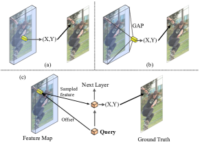
Regression-based pose-estimation has received less attention than heatmap-based methods due to its inferior performance. There are a variety of causes of this performance deficit. First, in order to reduce the number of parameters in the final FC prediction layer, models such as DeepPose [31] and RLE [18] employ a global average pooling that is applied to reduce the CNN feature map’s resolution before the FC layers, as illustrated in Fig. 2(b). This global average pooling destroys the spatial structure of the convolutional feature maps, and has a significantly negative impact on performance. Next, as shown in Fig. 2(a), the convolutional features and predictions of some regression-based models (e.g. DirectPose [30] and SPM [26]) are misaligned, which consequently reduces localization precision. Lastly, regression-based methods only regress the coordinates of body joints and do not exploit the structured dependency between them [28].

Recently, Transformers have been applied to a range of tasks in computer vision, achieving impressive results [40, 12, 4]. This, and the fact that transformers were originally designed for sequence-to-sequence tasks, motivated our formulation of single person pose estimation as a sequence prediction problem. Specifically, we pose the problem as that of predicting a length-$K$ sequence of coordinates, where $K$ is the number of body joints for one person. This leads to a simple and novel regression-based pose estimation framework, that we label as Poseur.

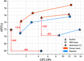
As shown in Fig. 3, taking as inputs the feature maps of an encoder CNN, the transformer predicts $K$ coordinate pairs. In doing so, Poseur alleviates the aforementioned difficulties of regression-based methods. First, it does not need global average pooling to reduce feature dimensionality (cf. RLE [18]). Second, Poseur eliminates the misalignment between the backbone features and predictions with the proposed efficient cross-attention mechanism. Third, since the self-attention module is applied across the keypoint queries, the transformer naturally captures the structured dependencies among the keypoints. Lastly, as shown in Fig. 2, Poseur outperforms heatmap-based methods with a variety of backbones. The improvement is more significant for the backbones using low-resolution representation, e.g., MobileNet V2 and ResNet. The results indicate that Poseur can be deployed with fast backbones of low-resolution representation without large performance drop, which is difficult to be achieved for heatmap-based methods. We refer readers to Sec. 4.4 for more details.

Our main contributions are as follows.

• We propose a transformer-based framework (termed Poseur) for directly human pose regression, which is lightweight and can work well with the backbones using low-resolution representation. For example, with 49% fewer FLOPs, ResNet-50 based Poseur outperforms the heatmap-based method SimpleBaseline [36] by $5.0$ AP on the COCO val set.

• Poseur significantly improves the performance of regression-based methods, to the point where it is comparable to the state-of-the-art heatmap-based approaches. For example, it improves on the previously best regression-based method (RLE [18]) by $4.9$ AP with the ResNet-50 backbone on the COCO val set and outperforms the previously best heatmap-based method UDP-Pose [27] by $1.0$ AP with HRNet-W48 on the COCO test-dev set.

• Our proposed framework can be easily extended to an end-to-end pipeline without manual crop operation, for example, we integrate Poseur into Mask R-CNN [15], which is end-to-end trainable and can overcome many drawbacks of the heatmap-based methods. In this end-to-end setting, our method outperforms the previously best end-to-end top-down method PointSet Anchor [34] by $3.8$ AP with the HRNet-W48 backbone on the COCO val set.

2 Related Work

Heatmap-based pose estimation. Heatmap-based 2D pose estimation methods[6, 36, 27, 2, 21, 3, 7, 15, 25] estimate per-pixel likelihoods for each keypoint location, and currently dominate in the field of 2D human pose estimation. A few works [25, 27, 2] attempt to design powerful backbone networks which can maintain high-resolution feature maps for heatmap supervision. Another line of works [28, 39, 17] focus on alleviating biased data processing pipeline for heatmap-based methods. Despite the good performance, the heatmap representation bears a few drawbacks in nature, e.g. , non-differentiable decoding pipeline [29, 30] and quantization errors [17, 39] due to the down sampling of feature maps.

Regression-based pose estimation. 2D human pose estimation is naturally a regression problem[29]. However, regression-based methods have historically not been as accurate as heatmap-based methods, and it has received less attention as a result[31, 29, 28, 5, 30, 26]. Integral Pose [29] proposes integral regression, which shares the merits of both heatmap representation and regression approaches, to avoid non-differentiable post-processing and quantization error issues. However, integral regression is proven to have an underlying bias compared with direct regression according to [14]. RLE [18] develops a regression-based method using maximum likelihood estimation and flow models. RLE [18] is the first to push the performance of the regression-based method to a level comparable with that of the heatmap-based methods. However, it is trained on the backbone that pre-trained by the heatmap loss.

Transformer-based architectures. Transformers have been applied to the pose estimation task with some success. TransPose [37] and HRFormer [38] enhance the backbone via applying the Transformer encoder to the backbone; TokenPose [22] designs the pose estimation network in a ViT-style fashion by splitting image into patches and applying class tokens, which makes the pose estimation more explainable. These methods are all heatmap-based and use a heavy transformer encoder to improve the model capacity. In contrast, Poseur is a regression-based method with a lightweight transformer decoder. Thus, Poseur is more computational efficient while can still achieve high performance.

PRTR [20] leverage the encoder-decoder structure in transformers to perform pose regression. PRTR is based on DETR [4], i.e., it uses Hungarian matching strategy to find a bipartite matching between non class-specific queries and ground-truth joints. It brings two issues: 1) heavy computational cost; 2) redundant queries for each instance. In contrast, Poseur can alleviate both issues while achieving much higher performance.

3 Method

Figure 3: The architecture of Poseur. The model directly predicts a sequence of keypoint coordinates in parallel by combining (a) backbone network with (b) keypoint encoder and (c) query decoder. (d) Residual Log-likelihood Estimation [18]. (e) The proposed uncertainty score for our method.

3.1 Poseur Architecture

Our proposed pose estimator Poseur aims to predict $K$ human keypoint coordinates from a cropped single person image. As shown in Fig. 2(c), The core idea of our method is to represent human keypoints with queries, i.e., each query corresponds to a human keypoint. The queries are input to the deformable attention module [40], which adaptively attends to the image features that most relevant to the query/keypoint. In this way, the information about a specific keypoint can be summarized and encoded into a single query, which is used to regress the keypoint coordinate later. As such, the issue of losing spatial information caused by the global average pooling in RLE [19] (As shown in Fig. 2(b)) is well addressed.

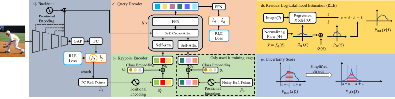
Specifically, in Poseur framework (shown in Fig. 3), two main components are added upon the backbone: a keypoint encoder and a query decoder. An input image is first encoded as dense feature maps with the backbone, which are followed by an FC layer to predict the rough keypoint coordinates, used as a set of rough proposals. We denote the proposal coordinates as ${\hat{\mathbf{{\boldsymbol{\mu}}}}_{f}}\in{\mathbb{R}}^{K\times 2}$. Then, those proposals are used to initialize the keypoint-specific query $\mathbf{Q}\in{\mathbb{R}}^{K\times C}$ (where $C$ is the embedding dimension) in the keypoint encoder. Finally, the feature maps from the backbone and $\mathbf{Q}$ are sent into the query decoder to obtain the final features for the keypoints, each of which is sent into a linear layer to predict the corresponding keypoint coordinates. In addition, unlike previous methods simply regressing the keypoint coordinates and applying the $L_{1}$ loss for supervision, Poseur, following RLE  [19], predicts a probability distribution reflecting the probability of the ground truth appearing in each location and supervise the network by maximum the probability on the ground truth location. Specifically, a location parameter ${\hat{\mathbf{{\boldsymbol{\mu}}}}_{q}}$ and a scale parameter ${\hat{\mathbf{{\boldsymbol{b}}}}_{q}}$ are predicted by Poseur ($\Theta$) for shifting and scaling the distribution generated by a flow model $\Phi$ (refer to Sec. 3.2). ${\hat{\mathbf{{\boldsymbol{\mu}}}}_{q}}$ is the center of the distribution and can be regarded as the predicted keypoint coordinates.

Backbone. Our method is applicable to both CNN (e.g. ResNet [16], HRNet [27]) and transformer backbones (e.g. HRFormer [38]). Given the backbone, multi-level feature maps are extracted and then fed into the query decoder. At the same time, a global average pooling operation is conducted in the last stage of the backbone and followed by an FC layer to regress the coarse keypoint coordinates ${\hat{\mathbf{{\boldsymbol{\mu}}}}_{f}}$ (normalized in $[0,1]$) and the corresponding scale parameter ${\hat{\mathbf{{\boldsymbol{b}}}}_{f}}$, supervised by Residual Log-Likelihood Estimation (RLE) process introduced in Sec. 3.2.

Keypoint encoder. The keypoint encoder is used to initialize each query $\mathbf{Q}$ for the query decoder. For initializing the query better, two keypoints’ attributes, location and category, are encoded into the query in the keypoint encoder. Specifically, first, for location attribute, we encode the rough x-y keypoint coordinates ${\hat{\mathbf{{\boldsymbol{\mu}}}}_{f}}$ with the fixed positional encodings, transforming the x-y coordinates to the sine-cosine positional embedding following  [32]. The obtained tensor is denoted by ${\hat{\mathbf{{\boldsymbol{\mu}}}}_{f}}^{*}\in{\mathbb{R}}^{K\times C}$; second, for the category attribute, $K$ learnable vectors ${{\mathbf{Q}}_{c}}\in{\mathbb{R}}^{K\times C}$, called class embedding, is used to represent K different categories separately. Finally, the initial queries ${{\mathbf{Q}}_{z}}\in{\mathbb{R}}^{K\times C}$ are generated by fusing the location and category attribute through element-wise addition of the positional and class embedding, i.e.${{\mathbf{Q}}_{z}}={{\mathbf{Q}}_{c}}+{\hat{\mathbf{{\boldsymbol{\mu}}}}_{f}}^{*}$.

However, ${\hat{\mathbf{{\boldsymbol{\mu}}}}_{f}}$ is just a coarse proposal, which sometimes goes wrong during inference. To make our model more robust for the wrong proposal, we introduce a query augmentation process, named noisy reference points sampling strategy, used only during training. The core idea of noisy reference points sampling strategy is to simulate the case that the coarse proposals ${\hat{\mathbf{{\boldsymbol{\mu}}}}_{f}}$ goes wrong and force the decoder to located correct keypoint with wrong proposal. Specifically, during training, we construct two types of keypoint queries. The first type of keypoint query is initialized with the proposal ${\hat{\mathbf{{\boldsymbol{\mu}}}}_{f}}$; the second type of keypoint query is initialized with normalized random coordinates ${\hat{\mathbf{{\boldsymbol{\mu}}}}_{n}}$ (noisy proposal). And then, both of two types query are processed equally in all following training stages. Our experiment shows that training the decoder network with noisy proposal ${\hat{\mathbf{{\boldsymbol{\mu}}}}_{n}}$ improves its robustness to errors introduced by coarse proposal ${\hat{\mathbf{{\boldsymbol{\mu}}}}_{f}}$ during the inference stage. Note, that during inference randomly initialized keypoint queries are not used.

Query decoder. In query decoder, query and feature map are mainly used to module the relationship between keypoints and input image. As shown in Fig. 3, the decoder follows the typical transformer decoder paradigm, in which, there are N identical layers in the decoder, each layer consisting of self-attention, cross-attention and feed-forward networks (FFNs). The query $\mathbf{Q}$ goes through these modules sequentially and generates an updated $\mathbf{Q}$ as the input to the next layer. As in DETR[4], the self-attention and FFNs are a multi-head self-attention [32] module and MLPs, respectively. For the cross-attention networks, we propose an efficient multi-scale deformable attention (EMSDA) module, based on MSDA proposed by Deformable DETR [40]. Similar to MSDA, in EMSDA, each query learns to sample relevant features from the feature maps by given the sampling offset around a reference point (a pair of coordinates, and which will be introduced later); and then, the sampled features are summarized by the attention mechanism to update the query. Different from MSDA, which applies a linear layer to the entire feature maps and thus is less efficient, we found that it is enough to only apply the linear layer to the sampled features after bilinear interpolation. Experiments show that the latter can have a similar performance while being much more efficient. Specifically, EMSDA can be written as

$$\operatorname{EMSDA}({\mathbf{Q}}_{q},\hat{{\mathbf{p}}}_{q},\{{\mathbf{x}}^{l}\}_{l=1}^{L})=\operatorname{Concat}(\text{head}_{\mathrm{1}},\ldots,\text{head}_{\mathrm{M}}){\mathbf{W}}^{o}$$ (1)

$$\text{where}\ \ \text{head}_{\mathrm{i}}=(\sum\limits_{l=1}^{L}{\sum\limits_{s=1}^{S}{{\mathbf{A}}_{i,l,q,s}\cdot{\mathbf{x}}^{l}(\phi_{l}(\hat{{\mathbf{p}}}_{q})+\Delta{p_{i,l,q,s}})}}){\mathbf{W}}^{v}_{i},$$

where ${\mathbf{Q}}_{q}\in{\mathbb{R}}^{C}$, $\hat{{\mathbf{p}}}_{q}\in{\mathbb{R}}^{2}$ and $\{{\mathbf{x}}^{l}\}_{l=1}^{L}$ are the $q$-th input query vector, the reference point offset of $q$-th query and $l$-th level of feature maps from the backbone; the dimension of each feature vector in ${\mathbf{x}}$ is $C$. $\text{head}_{i}$ represents $i$-th attention head. $L$, $M$ and $S$ represent the number of feature map levels used in the decoder, the number of attention heads and the number of sampling points on each level feature map, respectively. ${\mathbf{A}}_{i,l,q,s}\in{\mathbb{R}}^{1}$ and $\Delta{p_{i,l,q,s}}\in{\mathbb{R}}^{2}$ represent the attention weights and the sampling offsets of the $i$-th head, $l$-th level, $q$-th query and $s$-th sampling point, respectively; The query feature ${\mathbf{Q}}_{q}$ is fed to a linear projection to generate ${\mathbf{A}}_{i,l,q,s}$ and $\Delta{p_{i,l,q,s}}$. ${\mathbf{A}}_{i,l,q,s}$ satisfies the limitation, $\sum\limits_{l=1}^{L}{\sum\limits_{s=1}^{S}{{\mathbf{A}}_{i,l,q,s}}}=1$. $\phi_{l}(\cdot)$ is the function transforming the $\hat{{\mathbf{p}}}_{q}$ to the coordinate system of the $l$-th level features. ${\mathbf{x}}^{l}(\phi_{l}(\hat{{\mathbf{p}}}_{q})+\Delta{p_{i,l,q,s}})$ represents sampling the feature vector located in offset $(\phi_{l}(\hat{{\mathbf{p}}}_{q})+\Delta{p_{i,l,q,s}})$ on the feature map ${\mathbf{x}}^{l}$ by bilinear interpolation. ${\mathbf{W}}^{o}\in{\mathbb{R}}^{C\times C}$ and ${\mathbf{W}}^{v}_{i}\in{\mathbb{R}}^{C\times(C/M)}$ are two groups of trainable weights. The reference point $\hat{{\mathbf{p}}}_{q}$ will be updated at the end of each decoder layer by applying a linear layer on ${\mathbf{Q}}_{q}$. Note, the FC output ${\hat{\mathbf{{\boldsymbol{\mu}}}}_{f}}$ is leveraged as reference point for the initial query ${{\mathbf{Q}}_{z}}$. For more details and computational complexity, we refer readers to our supplementary material.

To sum up, the relations between different keypoints are modeled through a self-attention module, and the relations between the input image and keypoints are modeled through EMSDA module. Notably, the problem of feature misalignment in fully-connected regression is solved by EMSDA.

3.2 Training Targets and Loss Functions

Following RLE [18], we calculate a probability distribution $P_{{{\boldsymbol{\Theta}}},{{\boldsymbol{\Phi}}}}({\mathbf{x}}|\mathcal{I})$ reflecting the probability of the ground truth appearing in the location ${\mathbf{x}}$ conditioning on the input image $\mathcal{I}$, where ${\boldsymbol{\Theta}}$ is the parameters of Poseur and ${\boldsymbol{\Phi}}$ is the parameters of a flow model. As shown in Fig. 3(d), The flow model $f_{\phi}$ is leveraged to reflect the deviation of the output from the ground truth ${\boldsymbol{\mu}}_{g}$ by mapping a initial distribution $\bar{\textbf{z}}\sim\mathcal{N}(0,\mathbf{I})$ to a zero-mean complex distribution $\bar{\textbf{x}}\sim G_{\phi}(\bar{\textbf{x}})$. Then $P_{\phi}(\bar{{\mathbf{x}}})$ is obtained by adding a zero-mean Laplace distribution $L(\bar{{\mathbf{x}}})$ to $G(\bar{{\mathbf{x}}})$. The regression model ${\boldsymbol{\Theta}}$ predictions the center $\hat{{\boldsymbol{\mu}}}$, and scale $\hat{{\boldsymbol{b}}}$ of the distribution. Finally, the distribution $P_{{{\boldsymbol{\Theta}}},{{\boldsymbol{\Phi}}}}({\mathbf{x}}|\mathcal{I})$ is built upon $P_{\phi}(\bar{{\mathbf{x}}})$ by shifting and rescaling $\bar{{\mathbf{x}}}$ into ${\mathbf{x}}$, where ${\mathbf{x}}=\bar{{\mathbf{x}}}\cdot\hat{\boldsymbol{\sigma}}+\hat{{\boldsymbol{\mu}}}$. We refer readers to [18] for more details.

Different from RLE [18], we only use the proposal $(\hat{{\boldsymbol{\mu}}}_{f},\hat{\boldsymbol{b}}_{f})$ for coarse prediction. This prediction is then updated by the query-based approach described above to generate an improved estimate $(\hat{{\boldsymbol{\mu}}}_{q},\hat{\boldsymbol{b}}_{q})$. Both coarse proposal $(\hat{{\boldsymbol{\mu}}}_{f},\hat{\boldsymbol{b}}_{f})$ and query decoder preditions $(\hat{{\boldsymbol{\mu}}}_{q},\hat{\boldsymbol{b}}_{q})$ are supervised with the maximum likelihood estimation (MLE) process. The learning process of MLE optimizes the model parameters so as to make the observed ground truth ${\boldsymbol{\mu}}_{g}$ most probable. The loss function of FC predictions $(\hat{{\boldsymbol{\mu}}}_{f},\hat{\boldsymbol{b}}_{f})$ can be defined as:

$$\mathcal{L}_{rle}^{fc}=-\log P_{{{\boldsymbol{\Theta}}}_{f},{{\boldsymbol{\Phi}}}_{f}}({\mathbf{x}}|\mathcal{I})\Big{|}_{{\mathbf{x}}={\boldsymbol{\mu}}_{g}},$$ (2)

where ${\boldsymbol{\Theta}}_{f}$ and ${\boldsymbol{\Phi}}_{f}$ are the parameters of the backbone and flow model, respectively. Similarly, the loss of distribution associated with query decoder preditions $(\hat{{\boldsymbol{\mu}}}_{q},\hat{\boldsymbol{b}}_{q})$ can be defined as:

$$\mathcal{L}_{rle}^{dec}=-\log P_{{{\boldsymbol{\Theta}}}_{q},{{\boldsymbol{\Phi}}}_{q}}({\mathbf{x}}|\mathcal{I})\Big{|}_{{\mathbf{x}}={\boldsymbol{\mu}}_{g}},$$ (3)

where ${\boldsymbol{\Theta}}_{q}$ and ${\boldsymbol{\Phi}}_{q}$ are the parameters of the query decoder and another flow model, respectively. Finally, we sum the two loss functions to obtain the total loss:

$$\mathcal{L}_{total}=\mathcal{L}_{rle}^{fc}+\lambda\mathcal{L}_{rle}^{dec},$$ (4)

where $\lambda$ is a constant and used to balance the two losses. We set $\lambda=1$ by default.

3.3 Inference

Inference pipeline. During the inference stage, Poseur predicts the $(\hat{{\boldsymbol{\mu}}}_{q},\hat{{\boldsymbol{b}}}_{q})$ for each keypoint as mentioned; $\hat{{\boldsymbol{\mu}}}_{q}$ is taken as the predicted keypoint coordinates and $\hat{\boldsymbol{b}}_{q}$ is used to calculate the keypoint confidence score.

Prediction uncertainty estimation. For heatmap-based methods, e.g. SimpleBaseline [36], the prediction score of each keypoint is combined with a bounding box score to enhance the final human instance score:

$$\boldsymbol{s}^{inst}=\boldsymbol{s}^{bbox}\frac{\sum_{i=1}^{k}\boldsymbol{s}^{kp}_{i}}{K},$$ (5)

where $\boldsymbol{s}^{inst}$ is the final prediction score of the instance; $\boldsymbol{s}^{bbox}$ is the bounding box score predicted by the person detector, $\boldsymbol{s}_{i}^{kp}$ is the $i$-th keypoint score predicted by the keypoint detector and $K$ is the total keypoint number of each human. Most previous regression-based methods [31, 29] ignore the importance of the keypoint score. As a result, compared to heatmap based methods, regression methods typically achieve higher recall but lower precision. Given the same well-trained Poseur model, adding the keypoint score brings $4.7$ AP improvement ($74.7$ AP vs. $70.0$ AP) due to the significantly reduced number of false positives, and both of the models achieve almost the same average recall (AR).

Our model predicts a probability distribution over the image coordinates for each human keypoint. We define the $i$-th keypoint prediction score $\boldsymbol{s}^{kp}_{i}$ to be the probability of the keypoint falling into the region ($[\hat{{\boldsymbol{\mu}}}_{i}-\mathbf{a},\hat{{\boldsymbol{\mu}}}_{i}+\mathbf{a}]$) near the prediction coordinate $\hat{{\boldsymbol{\mu}}}_{i}$, i.e.

$$\boldsymbol{s}_{i}^{kp}=\int_{\hat{{\boldsymbol{\mu}}}_{i}-\mathbf{a}}^{\hat{{\boldsymbol{\mu}}}_{i}+\mathbf{a}}P_{{{\boldsymbol{\Theta}}}_{q},{{\boldsymbol{\Phi}}}_{q}}({\mathbf{x}}|\mathcal{I})dx,$$ (6)

where $\mathbf{a}$ is a hyperparameter that controls the size of the ${\boldsymbol{\mu}}$-adjacent interval, and $\hat{{\boldsymbol{\mu}}}_{i}$ are the coordinates of the corresponding keypoint predicted by Poseur. In practice, running the normalization flow model during the inference stage would add more computational cost. We found that comparable performance can be achieved by shifting and re-scaling the zero-mean Laplace distribution $L(\bar{{\mathbf{x}}})$ with query decoder predictions $(\hat{{\boldsymbol{\mu}}}_{q},\hat{\boldsymbol{b}}_{q})$. So the probability density function can be rewritten as:

$$P_{{{\boldsymbol{\Theta}}}_{q},{{\boldsymbol{\Phi}}}_{q}}({\mathbf{x}}|\mathcal{I})\approx f({\mathbf{x}}|\hat{{\boldsymbol{\mu}}}_{i},\hat{\boldsymbol{b}}_{i})=\frac{1}{2\hat{\boldsymbol{b}}_{i}}\exp{(-\frac{|{\mathbf{x}}-\hat{{\boldsymbol{\mu}}}_{i}|}{\hat{\boldsymbol{b}}_{i}})},$$ (7)

where $\hat{{\boldsymbol{\mu}}}_{i}$ is the center of the Laplacian distribution and the predicted keypoint coordinates, and $\hat{\boldsymbol{b}}_{i}$ is the scale parameter predicted by Poseur. Finally, $\boldsymbol{s}_{i}^{kp}$ can be written as:

$$\boldsymbol{s}_{i}^{kp}=\int_{\hat{{\boldsymbol{\mu}}}_{i}-\mathbf{a}}^{\hat{{\boldsymbol{\mu}}}_{i}+\mathbf{a}}f({\mathbf{x}}|\hat{{\boldsymbol{\mu}}}_{i},\hat{\boldsymbol{b}}_{i})dx=1-\exp{(-\frac{\mathbf{a}}{\hat{\boldsymbol{b}}_{i}})}.$$ (8)

Note that the score $\boldsymbol{s}_{i}^{kp}$ on x-axis and y-axis will be calculated separately and then merged by a multiplication operation.

4 Experiments

4.1 Implementation Details

Datasets. Our experiments are mainly conducted on COCO2017 Keypoint Detection[33] benchmark, which contains about $250K$ person instances with 17 keypoints. We report results on the val set for ablation studies and compare with other state-of-the-art methods on both of the val set and test-dev sets. The Average Precision (AP) based on Object Keypoint Similarity (OKS) is employed as the evaluation metric on COCO dataset. We also conduct experiments on MPII [1] dataset with Percentage of Correct Keypoint (PCK) as evaluation metric.

Model settings. Unless specified, ResNet-50[16] is used as the backbone in ablation study. The size of input image is $256\times 192$. The weights pre-trained on ImageNet[9] are used to initialize the ResNet backbone. The rest parts of our network are initialized with random parameters. All the decoder embedding size is set as 256; 3 decoder layers are used by default.

Training. All the models are trained with batch size 256 (batch size 128 for HRFormer-B due to the limited GPU memory), and are optimized by AdamW[23] with a base learning rate of $1\times 10^{-3}$ decreased to $1\times 10^{-4}$ and $1\times 10^{-5}$ at the 255-th epoch and 310-th epoch and ended at the 325-th epoch; $\beta_{1}$ and $\beta_{2}$ are set to $0.9$ and $0.999$, respectively; Weight decay is set to $10^{-4}$. Following Deformable DETR [40], the learning rate of the the linear projections for sampling offsets and reference points are multiplied by a factor of $0.1$. Following RLE [18], we adopt RealNVP [11] as the flow model. Other settings follow that of mmpose [8]. For HRNet-W48 and HRFormer-B, cutout [10] and color jitter augmentation are applied to avoid over-fitting.

Inference. Following conventional settings, we use the same person detector as in SimpleBaseline [36] for COCO evaluation. According to the bounding box generated by the person detector, the single person image patch is cropped out from the original image and resized to a fix resolution, e.g. $256\times 192$. The flow model is removed during the inference. We set $\mathbf{a}=0.2$ in Eq. 7 by default.

4.2 Ablation Study

Initialization of keypoint queries. We conduct experiments to verify the impact of initialization of keypoint queries. Deformable DETR [40] introduces reference points that represent the location information of object queries. In their paper, reference points are 2-d tensors predicted from the 256-d object queries via a linear projection. We set this configuration as our baseline model. As shown in  Table 1a, the baseline model achieves 72.3 AP with 3 decoder layers, which is $0.6$ AP lower than keypoint queries which initialized from coarse proposal ${\hat{\mathbf{{\boldsymbol{\mu}}}}_{f}}$. This indicates that coarse proposal ${\hat{\mathbf{{\boldsymbol{\mu}}}}_{f}}$ provide a good initialization for the keypoint queries.

Table 1: Ablation of proposed Poseur on COCO val2017 split. “Ours”: Using the fully convolutional layer at the end of backbone to regress the coarse proposal ${\hat{\mathbf{{\boldsymbol{\mu}}}}_{f}}$; “Noisy Reference Points”: applying the noisy reference points sampling strategy in the keypoint encoder; “Res-$i$”: $i$-th level feature map of ResNet; “$N_{d}$”: the number of decoder layers

Initial Ref. Points	AP
Def. DETR[40]	72.3
Ours	72.9

(a) Varying Initial Reference Points Methods

Noisy Ref. Points	AP
✗	73.7
✓	74.3

(b) Varying the Noisy Reference Points

Uncertainty Esti.	AP
RLE [18]	73.6
Ours	74.7

(c) Varying the Uncertainty Estimation

Res2	Res3	Res4	Res5	Params	GFLOPs	AP
			✓	28.3M	4.12	73.7
		✓	✓	28.7M	4.18	74.2
	✓	✓	✓	28.9M	4.28	74.4
✓	✓	✓	✓	29.0M	4.48	74.7

(d) Varying the scale levels of input feature map for decoder

$N_{d}$	Params	GFLOPs	AP	AP50	AP75
3	28.8M	4.48	74.7	90.2	81.6
4	30.2M	4.51	75.3	90.5	82.1
5	31.6M	4.54	75.4	90.3	82.2
6	33.1M	4.57	75.4	90.5	82.2

(e) Varying the numbers of decoder layers

Noisy reference points sampling strategy. As mentioned in Sec. 3.1, we apply the noisy reference points sampling strategy during the training. To validate its effectiveness, we perform ablation experiment on COCO, as show in  Table 1b. The experiment result shows that the noisy reference points sampling strategy can improve the accuracy by 0.6 AP without adding any extra computational cost during inference.

Varying the levels of feature map. We explore the impact of feeding different levels of backbone features into the proposed query decoder. As shown in Table 1d, the performance grows consistently with more levels of feature maps, e.g., 73.7 AP, 74.2 AP, 74.4 AP, 74.7 AP for 1, 2, 3, 4 levels of feature maps, respectively.

Uncertainty estimation. As mentioned in  Sec. 3.3, we redesign the prediction confidence score proposed in [18]. To study the effectiveness of the proposed score $\boldsymbol{s}^{kp}$, we compare it with predictions without re-score and predictions with RLE score [18] using the same model. As shown in Table 1c, the proposed method brings significant improvement (4.7 AP) to the model without uncertainty estimation, and outperforms the RLE score [18] by 1.0 AP.

Varying decoder layers. Here we study the effect of query decoder’s depth. Specifically, we conduct experiments by varying the number of decoder layers in Transformer decoder. As shown in  Table 1e, the performance grows at the first three layers and saturates at the sixth decoder layer.

Table 2: Comparison with heatmap methods by varying the backbone and the input resolution on the COCO val set. “SimBa”: SimpleBaseline [36]. For (a), the input resolution is 256$\times$192 and the number of decoder layers is 5. For (b), we use ResNet-50 as backbone and the number of decoder layers is 3.

Method	Backbone	GFLOPs	AP
SimBa.	MobileNet-V2	4.55	65.9
Poseur	MobileNet-V2	0.52	71.9
SimBa.	ResNet-50	8.27	72.4
Poseur	ResNet-50	4.54	75.4
HRNet	HRNet-W32	7.68	75.0
Poseur	HRNet-W32	7.95	76.9

(a) Varying the backbone

Method	Input size	Params	GFLOPs	AP
SimBa. [36]	64$\times$64	34.0M	0.69	31.4
Poseur	64$\times$64	28.8M	0.49	47.9
SimBa. [36]	128$\times$128	34.0M	2.76	59.3
Poseur	128$\times$128	28.8M	1.55	67.1
SimBa. [36]	256$\times$192	34.0M	8.26	71.0
Poseur	256$\times$192	28.8M	4.48	74.7

(b) Varying the input resolution

Varying the input size. We conduct experiments to explore the robust of Poseur under different input resolutions. Table 2b compares Poseur with SimpleBaseline, showing that our method consistently outperforms SimpleBaseline in all input sizes. The results also indicate that heatmap-based method suffers larger performance drop with the low-resolution input. For example, the proposed method outperforms SimpleBaseline by 14.6 AP in 64$\times$64 input resolution.

4.3 Extensions: End-to-End Pose Estimation

Our framework can easily extend to end-to-end human pose estimation, i.e., detecting multi-person poses without the manual crop operation. With Poseur as a plug-and-play scheme, end-to-end top-down keypoint detectors can obtain additional improvement. Here, we take Mask-RCNN as example to show the superiority of our method. The original keypoint head of Mask R-CNN is stacked 8 convolutional layers, followed by a deconv layer and 2× bilinear upscaling, producing an output resolution of 56$\times$56. We replace the deconv layer by an average pooling layer and an FC layer like [18]. The output of the FC layer is used to produce initial coarse proposal ${\hat{\mathbf{{\boldsymbol{\mu}}}}_{f}}$. Then coarse proposal ${\hat{\mathbf{{\boldsymbol{\mu}}}}_{f}}$ is feed into the keypoint encoder and query decoder as described in Sec. 3.1. We randomly sample 600 queries per image for training efficiency. Note that we conduct EMSDA on multi-scale backbone feature maps, rather than on ROI features. The output of FC layer and transformer decoder are both supervised with RLE loss [18]. We perform scale jittering [13] with random crops during training. We train the entire network for 180,000 iterations, with a batchsize of 32 in total. Other parameters are the same as the Detectron2 [35]. As shown in Table 4, Poseur outperforms the heatmap-based Mask R-CNN with ResNet 101 by 1.9 AP. Poseur outperforms the state-of-the-art regression-based method, PointSet Anchor with HRNet-W48 by $3.8$ AP.

Table 3: Comparison with end-to-end top-down methods on the COCO val set. ^† denote flipping and multi-sacle testing. Reg: regression-based approach; HM: heatmap-based approach

Method	Backbone	Type	AP	AP50	AP75
PRTR [20]	HRNet-W48	Reg.	64.9	87.0	71.7
Mask R-CNN [15]	ResNet-101	HM.	66.0	86.9	71.5
Mask R-CNN + RLE [18]	ResNet-101	Reg.	66.7	86.7	72.6
PointSet Anchor† [34]	HRNet-W48	Reg.	67.0	87.3	73.5
Mask R-CNN + Poseur	ResNet-101	Reg.	68.6	87.5	74.8
Mask R-CNN + Poseur	HRNet-W48	Reg.	70.1	88.0	76.5
Mask R-CNN + Poseur †	HRNet-W48	Reg.	70.8	87.9	77.0

Table 4: Comparisons on MPII validation set (PCKh@0.5). SimBa: SimpleBaseline [36]. Reg: regression-base approach; HM: heatmap-based approach

Method	Backbone	Type	Mean
SimBa. [36]	ResNet-152	HM.	$89.6$
HRNet [27]	HRNet-W32	HM.	$90.1$
TokenPose [22]	L/D$24$	HM.	${90.2}$
Integral [29]	ResNet-101	Reg.	87.3
PRTR [20]	HRNet-W32	Reg.	89.5
Poseur	HRNet-W32	Reg.	90.5

Table 5: Comparisons with state-of-the-art methods on the COCO val set. Input size and the GFLOPs are calculated under top-down single person pose estimation setting. Unless specified, the number of decoder layers is set to 6. “3 Dec.”: three decoder layers.

Method	Backbone / Type	Input Size	GFLOPs	APkp	AP${}^{kp}_{50}$	AP${}^{kp}_{75}$	AP${}^{kp}_{M}$	AP${}^{kp}_{L}$
Heatmap-based methods
SimBa. [36]	ResNet-50	$256\times 192$	8.9	70.4	88.6	78.3	67.1	77.2
SimBa. [36]	ResNet-152	$256\times 192$	15.7	72.0	89.3	79.8	68.7	78.9
HRNet [27]	HRNet-W32	$256\times 192$	7.1	74.4	90.5	81.9	70.8	81.0
HRNet [27]	HRNet-W48	$384\times 288$	32.9	76.3	90.8	82.9	72.3	83.4
TransPose [37]	H-A6	$256\times 192$	21.8	75.8	-	-	-	-
TokenPose [22]	S-V2	$256\times 192$	11.6	73.5	89.4	80.3	69.8	80.5
TokenPose [22]	B	$256\times 192$	5.7	74.7	89.8	81.4	71.3	81.4
TokenPose [22]	L/D6	$256\times 192$	9.1	75.4	90.0	81.8	71.8	82.4
TokenPose [22]	L/D24	$256\times 192$	11.0	75.8	90.3	82.5	72.3	82.7
HRFormer [38]	HRFormer-T	$256\times 192$	1.3	70.9	89.0	78.4	67.2	77.8
HRFormer [38]	HRFormer-S	$256\times 192$	2.8	74.0	90.2	81.2	70.4	80.7
HRFormer [38]	HRFormer-B	$256\times 192$	12.2	75.6	90.8	82.8	71.7	82.6
HRFormer [38]	HRFormer-B	$384\times 288$	26.8	77.2	91.0	83.6	73.2	84.2
UDP-Pose [17]	HRNet-W32	$256\times 192$	7.2	76.8	91.9	83.7	73.1	83.3
UDP-Pose [17]	HRNet-W48	$384\times 288$	33.0	77.8	92.0	84.3	74.2	84.5
Regression-based methods
PRTR [20]	ResNet-50	$384\times 288$	11.0	68.2	88.2	75.2	63.2	76.2
PRTR [20]	HRNet-W32	$384\times 288$	21.6	73.1	89.4	79.8	68.8	80.4
PRTR [20]	HRNet-W32	$512\times 384$	37.8	73.3	89.2	79.9	69.0	80.9
RLE [19]	ResNet-50	$256\times 192$	4.0	70.5	88.5	77.4	-	-
RLE [19]	HRNet-W32	$256\times 192$	7.1	74.3	89.7	80.8	-	-
Ours	MobileNet-v2	$256\times 192$	0.5	71.9	88.9	78.6	65.2	74.3
Ours	ResNet-50	$256\times 192$	4.6	75.4	90.5	82.2	68.1	78.6
Ours	ResNet-152	$256\times 192$	11.9	76.3	91.1	83.3	69.1	79.5
Ours	HRNet-W32	$256\times 192$	7.4	76.9	91.0	83.5	70.1	79.7
Ours	HRNet-W48	$384\times 288$	33.6	78.8	91.6	85.1	72.1	81.8
Ours (3 Dec.)	HRFormer-T	$256\times 192$	1.4	74.3	90.1	81.4	67.5	76.9
Ours (3 Dec.)	HRFormer-S	$256\times 192$	3.0	76.6	91.0	83.4	69.8	79.4
Ours	HRFormer-B	$256\times 192$	12.6	78.9	92.0	85.7	72.3	81.7
Ours	HRFormer-B	$384\times 288$	27.4	79.6	92.1	85.9	72.9	82.9

Table 6: Comparison with top-down methods on the COCO test-dev set. The proposed paradigm outpeforms heatmap-based methods in various settings. The input resolution of all methods is $384\times 288$.

Method	Backbone	APkp	AP${}^{kp}_{50}$	AP${}^{kp}_{75}$	AP${}^{kp}_{M}$	AP${}^{kp}_{L}$
Heatmap-based methods
SimBa† [36]	ResNet-152	73.7	91.9	81.1	70.3	80.0
HRNet† [27]	HRNet-W32	74.9	92.5	82.8	71.3	80.9
HRNet† [27]	HRNet-W48	75.5	92.5	83.3	71.9	81.5
TokenPose [22]	L/D24	75.9	92.3	83.4	72.2	82.1
HRFormer [38]	HRFormer-B	76.2	92.7	83.8	72.5	82.3
UDP-Pose [17]	HRNet-W48	76.5	92.7	84.0	73.0	82.4
Regression-based methods
PRTR [20]	ResNet-101	68.8	89.9	76.9	64.7	75.8
PRTR [20]	HRNet-W32	71.7	90.6	79.6	67.6	78.4
RLE [19]	ResNet-152	74.2	91.5	81.9	71.2	79.3
RLE [19]	HRNet-W48	75.7	92.3	82.9	72.3	81.3
Ours (6 Dec.)	HRNet-W48	77.6	92.9	85.0	74.4	82.7
Ours (6 Dec.)	HRFormer-B	78.3	93.5	85.9	75.2	83.4

4.4 Main Results

Gains on low-resolution backbone. In this part, we show the great improvement of Poseur on non-HRNet paradigm backbone which encode the input image as low-resolution representation. All models and training settings are tightly aligned. The input resolution of all models is $256\times 192$.

In Table 2a, Poseur with ResNet-50 significantly outperforms SimpleBaseline, and it is even higher than HRNet-W32, while the computational cost is much lower. Apart from that, Poseur with the lightweight backbone MobileNet-V2 can achieve comparable performance with SimpleBaseline using ResNet-50 backbone. In contrast, the performance of the MobileNet-V2 based SimpleBaseline is much worse, $6.0$ AP lower than our method with the same backbone. It is worth noting that the computational cost of Poseur with MobileNet-V2 is only about one-ninth that of SimpleBaseline with the same backbone.

Comparison with the state-of-the-art methods. We compare the proposed Poseur with state-of-the-art methods on COCO and MPII dataset. Poseur outperforms all regression-based and heatmap-based methods when using the same backbone, and achieves state-of-the-art performance with HRFormer-B backbone, i.e., $79.6$ AP on the COCO val set and $78.3$ AP on the COCO test-dev set. Poseur with HRFormer-B can even outperform the previous state-of-the-art UDP-Pose ($384\times 288$) by 1.1 AP on the COCO val set, when using lower input resolution ($256\times 192$). Quantitative results are reported in Table 5 and Table 6. On the MPII val set, Poseur with HRNet-W32 is 0.4 PCKh higher than heatmap-based method with HRNet-W32. Quantitative results are reported in Table 4.

5 Conclusion

We have proposed a novel pose estimation framework named Poseur built upon Transformers, which largely improves the performance of the regression-based pose estimation and bypasses the drawbacks of heatmap-based methods such as the non-differentiable post-processing and quantization error. Extensive experiments on the MS-COCO and MPII benchmarks show that Poseur can achieve state-of-the-art performance among both regression-based methods and heatmap-based methods.

See pages - of supp.pdf

References

- [1] Andriluka, M., Pishchulin, L., Gehler, P., Schiele, B.: 2d human pose estimation: New benchmark and state of the art analysis. In: Proc. IEEE Conf. Comp. Vis. Patt. Recogn. pp. 3686–3693 (2014)
- [2] Cai, Y., Wang, Z., Luo, Z., Yin, B., Du, A., Wang, H., Zhang, X., Zhou, X., Zhou, E., Sun, J.: Learning delicate local representations for multi-person pose estimation. In: Proc. Eur. Conf. Comp. Vis. pp. 455–472. Springer (2020)
- [3] Cao, Z., Hidalgo, G., Simon, T., Wei, S.E., Sheikh, Y.: Openpose: realtime multi-person 2d pose estimation using part affinity fields. IEEE Trans. Pattern Anal. Mach. Intell. 43(1), 172–186 (2019)
- [4] Carion, N., Massa, F., Synnaeve, G., Usunier, N., Kirillov, A., Zagoruyko, S.: End-to-end object detection with transformers. In: Proc. Eur. Conf. Comp. Vis. pp. 213–229. Springer (2020)
- [5] Carreira, J., Agrawal, P., Fragkiadaki, K., Malik, J.: Human pose estimation with iterative error feedback. In: Proc. IEEE Conf. Comp. Vis. Patt. Recogn. pp. 4733–4742 (2016)
- [6] Chen, Y., Wang, Z., Peng, Y., Zhang, Z., Yu, G., Sun, J.: Cascaded pyramid network for multi-person pose estimation. In: Proc. IEEE Conf. Comp. Vis. Patt. Recogn. pp. 7103–7112 (2018)
- [7] Cheng, B., Xiao, B., Wang, J., Shi, H., Huang, T.S., Zhang, L.: Higherhrnet: Scale-aware representation learning for bottom-up human pose estimation. In: Proc. IEEE Conf. Comp. Vis. Patt. Recogn. pp. 5386–5395 (2020)
- [8] Contributors, M.: Openmmlab pose estimation toolbox and benchmark. https://github.com/open-mmlab/mmpose (2020)
- [9] Deng, J., Dong, W., Socher, R., Li, L.J., Li, K., Fei-Fei, L.: Imagenet: A large-scale hierarchical image database. In: Proc. IEEE Conf. Comp. Vis. Patt. Recogn. pp. 248–255. Ieee (2009)
- [10] DeVries, T., Taylor, G.W.: Improved regularization of convolutional neural networks with cutout. arXiv: Comp. Res. Repository (2017)
- [11] Dinh, L., Sohl-Dickstein, J., Bengio, S.: Density estimation using real NVP. In: Proc. Int. Conf. Learn. Representations (2017)
- [12] Dosovitskiy, A., Beyer, L., Kolesnikov, A., Weissenborn, D., Zhai, X., Unterthiner, T., Dehghani, M., Minderer, M., Heigold, G., Gelly, S., et al.: An image is worth 16x16 words: Transformers for image recognition at scale. arXiv: Comp. Res. Repository (2020)
- [13] Ghiasi, G., Cui, Y., Srinivas, A., Qian, R., Lin, T.Y., Cubuk, E., Le, Q., Zoph, B.: Simple copy-paste is a strong data augmentation method for instance segmentation. In: Proc. IEEE Conf. Comp. Vis. Patt. Recogn. pp. 2918–2928 (2021)
- [14] Gu, K., Yang, L., Yao, A.: Removing the bias of integral pose regression. In: Proc. IEEE Int. Conf. Comp. Vis. pp. 11067–11076 (2021)
- [15] He, K., Gkioxari, G., Dollár, P., Girshick, R.: Mask r-cnn. In: Proc. IEEE Int. Conf. Comp. Vis. pp. 2961–2969 (2017)
- [16] He, K., Zhang, X., Ren, S., Sun, J.: Deep residual learning for image recognition. In: Proc. IEEE Conf. Comp. Vis. Patt. Recogn. pp. 770–778 (2016)
- [17] Huang, J., Zhu, Z., Guo, F., Huang, G.: The devil is in the details: Delving into unbiased data processing for human pose estimation. In: Proc. IEEE Conf. Comp. Vis. Patt. Recogn. pp. 5700–5709 (2020)
- [18] Li, J., Bian, S., Zeng, A., Wang, C., Pang, B., Liu, W., Lu, C.: Human pose regression with residual log-likelihood estimation. In: Proc. IEEE Int. Conf. Comp. Vis. (2021)
- [19] Li, J., Bian, S., Zeng, A., Wang, C., Pang, B., Liu, W., Lu, C.: Human pose regression with residual log-likelihood estimation. In: Proc. IEEE Int. Conf. Comp. Vis. (2021)
- [20] Li, K., Wang, S., Zhang, X., Xu, Y., Xu, W., Tu, Z.: Pose recognition with cascade transformers. In: Proc. IEEE Conf. Comp. Vis. Patt. Recogn. pp. 1944–1953 (2021)
- [21] Li, W., Wang, Z., Yin, B., Peng, Q., Du, Y., Xiao, T., Yu, G., Lu, H., Wei, Y., Sun, J.: Rethinking on multi-stage networks for human pose estimation. arXiv: Comp. Res. Repository (2019)
- [22] Li, Y., Zhang, S., Wang, Z., Yang, S., Yang, W., Xia, S.T., Zhou, E.: TokenPose: Learning keypoint tokens for human pose estimation. In: Proc. IEEE Int. Conf. Comp. Vis. (2021)
- [23] Loshchilov, I., Hutter, F.: Decoupled weight decay regularization. In: Proc. Int. Conf. Learn. Representations (2019)
- [24] Luo, Z., Wang, Z., Huang, Y., Tan, T., Zhou, E.: Rethinking the heatmap regression for bottom-up human pose estimation. arXiv preprint arXiv:2012.15175 (2020)
- [25] Newell, A., Yang, K., Deng, J.: Stacked hourglass networks for human pose estimation. In: Proc. Eur. Conf. Comp. Vis. pp. 483–499. Springer (2016)
- [26] Nie, X., Feng, J., Zhang, J., Yan, S.: Single-stage multi-person pose machines. In: Proc. IEEE Int. Conf. Comp. Vis. pp. 6951–6960 (2019)
- [27] Sun, K., Xiao, B., Liu, D., Wang, J.: Deep high-resolution representation learning for human pose estimation. In: Proc. IEEE Conf. Comp. Vis. Patt. Recogn. pp. 5693–5703 (2019)
- [28] Sun, X., Shang, J., Liang, S., Wei, Y.: Compositional human pose regression. In: Proc. IEEE Int. Conf. Comp. Vis. pp. 2602–2611 (2017)
- [29] Sun, X., Xiao, B., Wei, F., Liang, S., Wei, Y.: Integral human pose regression. In: Proc. Eur. Conf. Comp. Vis. pp. 529–545 (2018)
- [30] Tian, Z., Chen, H., Shen, C.: Directpose: Direct end-to-end multi-person pose estimation. arXiv: Comp. Res. Repository (2019)
- [31] Toshev, A., Szegedy, C.: Deeppose: Human pose estimation via deep neural networks. In: Proc. IEEE Conf. Comp. Vis. Patt. Recogn. pp. 1653–1660 (2014)
- [32] Vaswani, A., Shazeer, N., Parmar, N., Uszkoreit, J., Jones, L., Gomez, A.N., Kaiser, L., Polosukhin, I.: Attention is all you need. In: Proc. Advances in Neural Inf. Process. Syst. pp. 5998–6008 (2017)
- [33] Wang, Z., Li, W., Yin, B., Peng, Q., Xiao, T., Du, Y., Li, Z., Zhang, X., Yu, G., Sun, J.: Mscoco keypoints challenge 2018. In: Proc. Eur. Conf. Comp. Vis. vol. 5 (2018)
- [34] Wei, F., Sun, X., Li, H., Wang, J., Lin, S.: Point-set anchors for object detection, instance segmentation and pose estimation (2020)
- [35] Wu, Y., Kirillov, A., Massa, F., Lo, W.Y., Girshick, R.: Detectron2. https://github.com/facebookresearch/detectron2 (2019)
- [36] Xiao, B., Wu, H., Wei, Y.: Simple baselines for human pose estimation and tracking. In: Proc. Eur. Conf. Comp. Vis. pp. 466–481 (2018)
- [37] Yang, S., Quan, Z., Nie, M., Yang, W.: TransPose: Keypoint localization via Transformer. In: Proc. IEEE Int. Conf. Comp. Vis. (2021)
- [38] Yuan, Y., Fu, R., Huang, L., Lin, W., Zhang, C., Chen, X., Wang, J.: HRFormer: High-resolution transformer for dense prediction. In: Proc. Advances in Neural Inf. Process. Syst. (2021)
- [39] Zhang, F., Zhu, X., Dai, H., Ye, M., Zhu, C.: Distribution-aware coordinate representation for human pose estimation. In: Proc. IEEE Conf. Comp. Vis. Patt. Recogn. (June 2020)
- [40] Zhu, X., Su, W., Lu, L., Li, B., Wang, X., Dai, J.: Deformable DETR: Deformable Transformers for end-to-end object detection. In: Proc. Int. Conf. Learn. Representations (2021)