Refined normal approximations for the central and noncentral chi-square distributions and some applications

Abstract

In this paper, we prove a local limit theorem for the chi-square distribution with $r>0$ degrees of freedom and noncentrality parameter $\lambda\geq 0$. We use it to develop refined normal approximations for the survival function. Our maximal errors go down to an order of $r^{-2}$, which is significantly smaller than the maximal error bounds of order $r^{-1/2}$ recently found by Horgan & Murphy, (2013) and Seri, (2015). Our results allow us to drastically reduce the number of observations required to obtain negligible errors in the energy detection problem, from $250$, as recommended in the seminal work of Urkowitz, (1967), to only $8$ here with our new approximations. We also obtain an upper bound on several probability metrics between the central and noncentral chi-square distributions and the standard normal distribution, and we obtain an approximation for the median that improves the lower bound previously obtained by Robert, (1990).

This manuscript was accepted for publication in Statistics (Taylor & Francis). This version may differ from the published version (doi:10.1080/02331888.2022.2084544) in typographic details.

1 Introduction

For any $r>0$ and $\lambda\geq 0$, the density function of the central and noncentral chi-square distribution $\chi_{r}^{2}(\lambda)$ is defined by

$$f_{r,\lambda}(x) =\begin{cases}\frac{(x/2)^{r/2-1}}{2e^{(x+\lambda)/2}},&\mbox{if }\lambda=0~{}~{}(\text{central}),\\ \frac{1}{2}e^{-(x+\lambda)/2}\left(\frac{x}{\lambda}\right)^{(r/2-1)/2}I_{r/2-1}(\sqrt{\lambda x}),&\mbox{if }\lambda>0~{}~{}(\text{noncentral}),\end{cases}$$ (1.1)

$$=\frac{(x/2)^{r/2-1}}{2e^{(x+\lambda)/2}}\sum_{j=0}^{\infty}\frac{(\lambda x/4)^{j}}{j!\,\Gamma(r/2+j)},\quad x>0,$$

using the convention $0^{0}\vcentcolon=1$, and where $I_{\nu}$ denotes the modified Bessel function of the first kind of order $\nu$. The special case $\lambda=0$ corresponds to the central chi-square distribution. Sometimes we refer to the chi-square distribution to include the central and noncentral cases all at once. When $r=n\in\mathbb{N}$, the expression in (1.1) corresponds to the density function of $X=\sum_{i=1}^{n}Z_{i}^{2}$, where $Z_{i}\sim\mathcal{N}(\mu_{i},1)$, and the noncentrality parameter $\lambda$ satisfies $\lambda=\sum_{i=1}^{n}\mu_{i}^{2}$. For all $r>0$, the mean and variance of $X\sim\chi_{r}^{2}(\lambda)$ are well known to be

$$\mathbb{E}[X]=r+\lambda\qquad\text{and}\qquad\mathbb{V}\mathrm{ar}(X)=2(r+2\lambda),$$ (1.2)

see, e.g., (Johnson et al.,, 1995, Chapter 29, Section 4).

The first goal of our paper (Lemma 3.1) is to establish a local asymptotic expansion for the ratio of the central and noncentral chi-square density (1.1) to the normal density with the same mean and variance, namely:

$$\frac{1}{\sqrt{2(r+2\lambda)}}\phi(\delta_{x}),\quad\text{where}~{}~{}\phi(z)\vcentcolon=\frac{e^{-z^{2}/2}}{\sqrt{2\pi}}~{}~{}\text{and}~{}~{}\delta_{x}\vcentcolon=\frac{x-(r+\lambda)}{\sqrt{2(r+2\lambda)}}.$$ (1.3)

In Horgan & Murphy, (2013) and Seri, (2015), the authors derived the following two uniform bounds on a basic approximation of the survival function of the $\chi_{r}^{2}(\lambda)$ distribution using the survival function of the standard normal distribution, respectively,

$$\max_{a\in\mathbb{R}}\Big{|}\int_{a}^{\infty}f_{r,\lambda}(x){\rm d}x-\int_{a}^{\infty}\frac{1}{\sqrt{2(r+2\lambda)}}\phi(\delta_{x}){\rm d}x\Big{|}\leq\frac{1}{\sqrt{9\pi r}}+\frac{\widetilde{C}_{0}}{r},\quad\text{as }r\to\infty,$$ (1.4)

$$\max_{a\in\mathbb{R}}\Big{|}\int_{a}^{\infty}f_{r,\lambda}(x){\rm d}x-\int_{a}^{\infty}\frac{1}{\sqrt{2(r+2\lambda)}}\phi(\delta_{x}){\rm d}x\Big{|}$$

$$\qquad\lessapprox\frac{(r+4\lambda)}{\pi W(1)(r+2\lambda)^{2}}\left(1+\frac{r^{2}}{32}\binom{r}{8}^{-1/4}\right)+\frac{(r+3\lambda)}{2\sqrt{\pi}(r+2\lambda)^{3/2}},\quad\text{for }r\geq 8,$$ (1.5)

where $\widetilde{C}_{0}>0$ is a universal constant, and $W(\cdot)$ is the Lambert $W$-function and $W(1)\simeq 0.5671433$. A much older reference, Wallace, (1959), derived a similar approximation with a maximal error of order $r^{-1/2}$ in the tails. The second goal in our paper is to refine those approximations significantly down to a maximal error of order $r^{-2}$. As a corollary, we can obtain an expansion for the percentage points (or quantiles) of the central and noncentral chi-square distributions in terms of the percentage points of the standard normal distribution. We will do so for the median in Section 4.2, where we improve a previous approximation given by Robert, (1990).

Here is a brief outline of the paper. In Section 2, we survey the literature on approximations of the cumulative distribution function (henceforth abbreviated by the acronym c.d.f.) and percentage points of the central and noncentral chi-square distribution. In Section 3, we present our main results, which include a local limit theorem for the central and noncentral chi-square distribution and corresponding approximations for the survival function (which improves the results in Horgan & Murphy, (2013) and Seri, (2015)). In Section 4, we present two applications of our main results: distance measure bounds between the chi-square distribution and the standard normal distribution, and the asymptotics of the median of the chi-square distribution. As mentioned above, the latter improves some results by Robert, (1990). The proofs of the main results are gathered in Appendix A, and some technical moment calculations are gathered in Appendix B.

Notation.

Throughout the paper, $u=\mathcal{O}(v)$ means that $\limsup_{r\to\infty}|u/v|<C$, where $C>0$ is a universal constant. Whenever $C$ might depend on some parameter, we add a subscript (for example, $u=\mathcal{O}_{\lambda}(v)$). Similarly, $u=\mathrm{o}(v)$ means that $\lim|u/v|=0$ as $r\to\infty$, and subscripts indicate which parameters the convergence rate can depend on.

2 Related works

In addition to the papers of Wallace, (1959), Horgan & Murphy, (2013) and Seri, (2015), several other works have discussed normal approximations to the central and/or noncentral chi-square distributions. We briefly mention some of them below. For a general reference, some of these approximations are surveyed in (Johnson et al.,, 1995, Chapter 29, Section 8). For the remainder of this section, $\Xi_{n}$ and $\Xi_{n,\lambda}$ (with $n\in\mathbb{N}$) will denote random variables distributed according to $\chi_{n}^{2}(0)$ and $\chi_{n}^{2}(\lambda)$, respectively.

Fisher, (1928) shows the approximate normality of a properly translated square root of a central chi-squared random variable, i.e.,

$$\sqrt{\Xi_{n}}-\sqrt{n-1}~{}~{}\text{is close in law to }\mathcal{N}(0,1),\quad\text{as }n\to\infty.$$ (2.1)

In a similar fashion, Wilson & Hilferty, (1931) show the approximate normality of properly translated third roots of central chi-squared random variables, i.e.,

$$\sqrt[3]{\Xi_{n}}-\sqrt[3]{n-2/3}~{}~{}\text{is close in law to }\mathcal{N}\left(0,\frac{2}{9}\sqrt[3]{\frac{1}{n-2/3}}\right),\quad\text{as }n\to\infty,$$ (2.2)

$$\sqrt[3]{\Xi_{n}/n}-\left(1-\frac{2}{9n}\right)~{}~{}\text{is close in law to }\mathcal{N}\left(0,\frac{2}{9n}\right),\quad\text{as }n\to\infty.$$ (2.3)

Merrington, (1941) compares numerically the percentage point approximations derived from the square root transformation of Fisher, (1928) and the third root transformation of Wilson & Hilferty, (1931), and he concludes that the latter is significantly more accurate. Germond & Hastings, (1944) develop various approximations for the c.d.f. of the noncentral chi-square distribution with two degrees of freedom, see (Johnson et al.,, 1995, p.466). Berkson, (1946) uses a method of “probits” and “logits” to approximate the chi-square distribution, showing the better approximation obtained by the logits. Patnaik, (1949) gives the following representation of the c.d.f. of the noncentral chi-square distribution:

$$\mathbb{P}(\Xi_{n,\lambda}\leq a)\leq\int_{0}^{a}\frac{e^{-(x+\lambda)/2}}{2^{n/2}}\sum_{j=0}^{\infty}\frac{x^{n/2+j-1}\lambda^{j}}{\Gamma(n/2+j)2^{2j}j!}{\rm d}x.$$ (2.4)

Patnaik presents many approximations for the c.d.f. One line of investigation suggests to approximate the above c.d.f. in terms of the central chi-square c.d.f. and to combine it with the approximation result of Fisher, which then enables a comparison between the noncentral chi-square c.d.f. and the standard normal c.d.f. Abdel-Aty, (1954) obtains approximate formulas for the percentage points and the c.d.f. of the noncentral chi-square distribution, using the first five cumulants of $(X/(r+\lambda))^{1/3}$, where $X\sim\chi_{r}^{2}(\lambda)$, expressed as series in inverse powers of $(r+\lambda)$ up to $(r+\lambda)^{-4}$. Sankaran, (1959) modifies Abdel-Aty’s method by taking $(X/(r+\lambda))^{h}$, for some $h$ that depends on $r$ and $\lambda$ and which makes the leading third cumulant of $(X/(r+\lambda))^{h}$ vanish. The objective was to make the distribution of $(X/(r+\lambda))^{h}$ more nearly normal than that of $(X/(r+\lambda))^{1/3}$. Results are given for a ‘first (normal) approximation’ and a ‘second approximation’, based on a Cornish-Fisher expansion. Tukey, (1957) presents an approximation for the 95% quantile of the noncentral chi-square distribution. Johnson, (1959) compares the c.d.f. approximations and corresponding percentage point (or quantile) approximations of Patnaik, (1949), Pearson, (1959) and others.

Severo & Zelen, (1960) gives an improved Wilson-Hilferty normalized deviate approximation to the chi-square distribution. Sankaran, (1963) examines a translated version of the third root transformation of a chi-squared random variable, namely $\sqrt[3]{(X-b)/(r+\lambda)}$ for $X\sim\chi_{r}^{2}(\lambda)$, and shows how the translation parameter $b$ can be chosen for the approximation to be as good as the ‘closer approximation’ of Abdel-Aty, (1954) for values of the noncentrality parameter that are not too small. Roy & Mohamad, (1964) give an approximation to the c.d.f. of the noncentral chi-square distribution in terms of central chi-square distributions, derived from a Laguerre series expansion of the density function. Their approximation add two corrective terms to the one in Patnaik, (1949), see also Tiku, (1965). Gray et al., (1969) uses the following expression to approximate the improper integral representation of the survival function of the central chi-square distribution:

$$\int_{a}^{\infty}f_{r,0}(x){\rm d}x$$ (2.5)

$$\approx\frac{e^{-(a-r)/2}}{(a/2-r/2+1)\sqrt{2\pi}}\left(\frac{a}{r}\right)^{r/2}\left(1-\frac{r/2-1}{(a/2-r/2+1)^{2}+a}\right)\left(\frac{12(r/2)^{3/2}}{6r+1}\right).$$

Robertson, (1969) gives the following formula

$$\int_{a}^{\infty}f_{r,\lambda}(x){\rm d}x$$ (2.6)

$$\approx\frac{e^{-\lambda/2}}{\Gamma(r/2)}\cdot\left[\begin{array}[]{l}\Gamma(r/2,a/2)+\frac{(\lambda/2)}{1!}\left\{\Gamma(r/2,a/2)+(a/r)(a/2)^{r/2-1}e^{-a/2}\right\}\\[2.84526pt] +\frac{(\lambda/2)^{2}}{2!}\left\{\Gamma(r/2,a/2)+\left(\frac{a}{r}+\frac{(a/2)^{2}}{r/2(r/2+1)}\right)(a/2)^{r/2-1}e^{-a/2}\right\}\\[5.69054pt] +\frac{(\lambda/2)^{3}}{3!}\left\{\begin{array}[]{l}\Gamma(r/2,a/2)\\ +\left(\frac{a}{r}+\frac{(a/2)^{2}}{r/2(r/2+1)}+\frac{(a/2)^{3}}{r/2(r/2+1)(r/2+2)}\right)(a/2)^{r/2-1}e^{-a/2}\end{array}\right\}\\ +\dots\end{array}\right]$$

for “accurate” approximations of the c.d.f. of the noncentral chi-square distribution over a wide range of degrees of freedom (even over 10,000).

In the same vein as Fisher and Wilson & Hilferty, Cressie & Hawkins, (1980) and Hawkins & Wixley, (1986) show the approximate normality of a properly translated fourth root of a chi-squared random variable. Chou et al., (1984) derive many new integral representations for the c.d.f. of the noncentral chi-square distribution; the numerical usefulness remains unclear. Bock & Govindarajulu, (1988) approximate the density and c.d.f. of a noncentral chi-square distribution using a table of modified Bessel functions. They give an exact expression when the degrees of freedom are odd. Dinges, (1989) presents two formulas to approximate the c.d.f. of the noncentral chi-square distribution, namely the following first and second order Wiener germ approximations:

$$\mathbb{P}(\Xi_{r,\lambda}\leq a)\approx\Phi\left(\pm\sqrt{\begin{array}[]{l}r(s-1)^{2}\left(\frac{1}{2s}+\mu^{2}-\frac{1}{s}h(1-s)\right)\\ -\log\left(\frac{1}{s}-\frac{2}{s}\cdot\frac{h(1-s)}{(1+2\mu^{2}s)}\right)+\frac{2(1+3\mu^{2})^{2}}{9r(1+2\mu^{2})^{3}}\end{array}}\right),$$ (2.9)

$$\mathbb{P}(\Xi_{r,\lambda}\leq a)\approx\Phi\left(\pm\sqrt{\begin{array}[]{l}r(s-1)^{2}\left(\frac{1}{2s}+\mu^{2}-\frac{1}{s}h(1-s)\right)\\ -\log\left(\frac{1}{s}-\frac{2}{s}\cdot\frac{h(1-s)}{(1+2\mu^{2}s)}\right)+\frac{2}{r}B(s)\end{array}}\right),$$ (2.12)

where

$$B(s) =-\frac{3}{2}\cdot\frac{(1+4\mu^{2}s)}{(1+2\mu^{2}s)^{2}}+\frac{5}{3}\cdot\frac{(1+3\mu^{2}s)^{2}}{(1+2\mu^{2}s)^{3}}+\frac{2(1+3\mu^{2}s)}{(s-1)(1+2\mu^{2}s)^{2}}$$ (2.13)

$$\quad+\frac{3\eta}{(s-1)^{2}(1+2\mu^{2}s)}-\frac{(1+2h(\eta))\eta^{2}}{2(s-1)^{2}(1+2\mu^{2}s)}.$$

and

$$h(y)=\begin{cases}\frac{1}{y^{2}}\left[(1-y)\log(1-y)+y-\frac{y^{2}}{2}\right],&\mbox{if }h\in(0,1),\\ 0,&\mbox{if }h=0,\end{cases}$$ (2.14)

$$\mu=\frac{\lambda}{r},\quad s=\frac{-1+\sqrt{1+(4x\mu^{2})/r}}{2\mu^{2}}~{}~{}\text{for some }x>0,$$

$$\eta=\frac{1+2\mu^{2}s-2h(1-s)-s-2\mu^{2}s^{2}}{1+2\mu^{2}s-2h(1-s)}.$$

The numerical implementation of these formulas is given by Penev & Raykov, (2000). Ashour & Abdel-Samad, (1990) give two computational approximations to the c.d.f. of the noncentral chi-square distribution of any degree of freedom and odd degrees of freedom respectively, using truncated infinite sums:

$$\mathbb{P}(\Xi_{n,\lambda}\leq a)=\frac{e^{-(a+\lambda)/2}(a/2)^{n/2}}{\Gamma(n/2+1)}\sum_{i=0}^{\infty}\frac{1}{i!}C_{i}(\lambda a/4,n/2)\sum_{s=0}^{\infty}C_{s}(a/2,n/2+i),$$ (2.15)

$$\qquad\text{where }C_{i}(\lambda a/4,n/2)=\frac{\lambda a/4}{n/2+i}C_{i-1}(\lambda a/4,n/2),\quad\text{for }i=1,2,3,\dots$$

$$\qquad\text{and }C_{0}(\lambda a/4,n/2)=1,$$

$$\mathbb{P}(\Xi_{2n+1,\lambda}>a)=\mathbb{P}(\Xi_{2n+1}>a)+\sqrt{\frac{2}{\pi}}e^{-a/2}\sum_{k=n+1}^{\infty}\frac{a^{k-1}}{(2k-1)!!}\mathbb{P}(\Xi_{2k-2n}\leq\lambda).$$ (2.16)

Robert, (1990) gives bounds on the quantiles of the noncentral chi-square distribution in terms of the noncentrality parameter. Increasing the accuracy requires shortening the range of the noncentrality parameter. Ding, (1992) gives an algorithm to compute the noncentral chi-square c.d.f. using a series representation based on a Poisson weighted sum of central chi-square c.d.f.s. Temme, (1993) gives two asymptotic expansions for the survival function of the noncentral chi-square distribution involving the survival function of the standard normal distribution, namely

$$\int_{a}^{\infty}f_{r,\lambda}(x){\rm d}x\sim 1-\left(\frac{a}{\lambda}\right)^{r/4-1/4}\Psi(\sqrt{r/2}-\sqrt{\lambda/2}),$$ (2.17)

$$\int_{a}^{\infty}f_{r,\lambda}(x){\rm d}x\sim\Psi\left(-u_{0}\sqrt{\frac{\lambda a}{2}}\right)+\phi\left(\frac{u_{0}}{\sqrt{\lambda a}}\right)\sum_{k=0}^{\infty}c_{2k}\frac{\Gamma(k+1/2)}{\Gamma(1/2)}\left(\frac{2}{\lambda a}\right)^{k},\quad\lambda a\to\infty,$$

for specific constants $u_{0},c_{0},c_{2},\dots$ given in (Temme,, 1993, p.60). Chattamvelli & Shanmugam, (1995) obtain an alternative error bound on Ruben’s algorithm (Ruben,, 1974) for the computation of the noncentral chi-square c.d.f. They also compare finite algorithms (such as Patnaik, (1949) and others) with the algorithms proposed by Ashour & Abdel-Samad, (1990) for such computation and they discuss the rates of convergence of two different series representations for the c.d.f. Fraser et al., (1998) uses third order asymptotic methods that only requires evaluation of the standard normal to approximate the c.d.f. of the noncentral chi-square distribution.

Canal, (2005) approximates the c.d.f. of a central chi-square distribution by considering a linear combination of fractional powers of a chi-squared random variable. The mean absolute error is shown to be lower than other power transformations (two of the most well known are the square root transformation by Fisher, (1922) and the third root transformation by Wilson & Hilferty, (1931)) for degrees of freedom $1\leq r\leq 1000$. Gaunt et al., (2017) uses Stein’s method to obtain an order $n^{-1}$ bound on the distributional distance over smooth test functions between Pearson’s statistics and its limiting chi-square distribution. Maširević, (2017) gives three formulas for the c.d.f. of the noncentral chi-square distribution in terms of modified Bessel functions, leaky aquifer functions, and generalized incomplete gamma functions, respectively. Okagbue et al., (2017) uses quantile mechanics methods to approximate the quantile density function (the derivative of the quantile function) and the corresponding quartiles of the chi-square distribution. The result of the method is a power series solution to an ordinary differential equation. Baricz et al., (2021) give various representations of the noncentral chi-square c.d.f. in terms of modified Bessel functions of the first kind, derived from two mean value theorems for definite integrals. Gaunt & Reinert, (2021) uses Stein’s method to obtain an order $n^{-1}$ bound on the distributional distance over smooth test functions between Friedman’s statistics and its limiting chi-square distribution.

For a discussion on the estimation of quadratic forms or the noncentrality parameter for a noncentral chi-square distribution, we refer the reader to de Waal, (1974), Perlman & Rasmussen, (1975), Neff & Strawderman, (1976), Anderson, (1981), Saxena & Alam, (1982), Spruill, (1986), Chow, (1987), Kubokawa et al., (1993), Shao & Strawderman, (1995), Johnstone, (2001b, a), Liu et al., (2009) and Kubokawa et al., (2017).

3 Main results

First, we need local approximations for the ratio of the noncentral chi-square density to the normal density function with the same mean and variance.

Lemma 3.1 (Local approximation).

For any $r>0$, $0\leq\lambda=\mathrm{o}(\sqrt{r})$ and $\eta\in(0,1)$, define

$$D_{r,\lambda}\vcentcolon=\frac{r+\lambda}{\sqrt{2(r+2\lambda)}},$$ (3.1)

and let

$$B_{r,\lambda}(\eta)\vcentcolon=\bigg{\{}x\in(0,\infty):\bigg{|}\frac{\delta_{x}}{D_{r,\lambda}}\bigg{|}\leq\eta\,r^{-1/3}\bigg{\}},$$ (3.2)

denote the bulk of the noncentral chi-square distribution. Then, uniformly for $k\in B_{r,\lambda}(\eta)$, we have, as $r\to\infty$,

$$\log\bigg{(}\frac{f_{r,\lambda}(x)}{\frac{1}{\sqrt{2(r+2\lambda)}}\phi(\delta_{x})}\bigg{)} =r^{-1/2}\,\bigg{\{}\frac{\sqrt{2}}{3}\,\delta_{x}^{3}-\sqrt{2}\,\delta_{x}\bigg{\}}+r^{-1}\,\bigg{\{}-\frac{1}{2}\,\delta_{x}^{4}+\delta_{x}^{2}-\frac{1}{6}\bigg{\}}$$

$$\quad+r^{-3/2}\,\bigg{\{}\frac{2^{3/2}}{5}\,\delta_{x}^{5}-\frac{2^{3/2}}{3}\,\delta_{x}^{3}\bigg{\}}+\mathcal{O}\bigg{(}\frac{(1\vee\lambda^{4})+\lambda^{2}|\delta_{x}|^{2}}{r^{2}}\bigg{)},$$ (3.3)

Furthermore,

$$\frac{f_{r,\lambda}(x)}{\frac{1}{\sqrt{2(r+2\lambda)}}\phi(\delta_{x})}=1 +r^{-1/2}\,\bigg{\{}\frac{\sqrt{2}}{3}\,\delta_{x}^{3}-\sqrt{2}\,\delta_{x}\bigg{\}}+r^{-1}\,\bigg{\{}\frac{1}{9}\,\delta_{x}^{6}-\frac{7}{6}\,\delta_{x}^{4}+2\,\delta_{x}^{2}-\frac{1}{6}\bigg{\}}$$

$$\quad+r^{-3/2}\,\bigg{\{}\frac{\sqrt{2}}{81}\,\delta_{x}^{9}-\frac{5}{9\sqrt{2}}\,\delta_{x}^{7}+\frac{47}{15\sqrt{2}}\,\delta_{x}^{5}-\frac{37}{9\sqrt{2}}\,\delta_{x}^{3}+\frac{1}{3\sqrt{2}}\,\delta_{x}\bigg{\}}$$

$$\quad+\mathcal{O}_{\eta}\bigg{(}\frac{(1\vee\lambda^{4})+|\delta_{x}|^{10}}{r^{2}}\bigg{)}.$$ (3.4)

For the interested reader, local approximations akin to Lemma 3.1 were derived for the Poisson, binomial, negative binomial, multinomial, Dirichlet, Wishart and multivariate hypergeometric distributions in (Ouimet,, 2021a, Lemma 2.1), (Ouimet,, 2022a, Lemma 3.1), (Ouimet,, 2021c, Lemma 2.1), (Ouimet,, 2021b, Theorem 2.1), (Ouimet,, 2022b, Theorem 1), (Ouimet,, 2022d, Theorem 1), (Ouimet,, 2022c, Theorem 1), respectively. See also earlier references such as Govindarajulu, (1965) (based on Fourier analysis results from Esseen, (1945)) for the Poisson, binomial and negative binomial distributions, and Cressie, (1978) for the binomial distribution.

By integrating the second local approximation in Lemma 3.1, we can approximate the survival function of the $\chi_{r}^{2}(\lambda)$ distribution, i.e.,

$$S_{r,\lambda}(a)\vcentcolon=\int_{a}^{\infty}f_{r,\lambda}(x){\rm d}x,\quad a\in\mathbb{R},$$ (3.5)

using the survival function of the normal distribution with the same mean and variance.

Theorem 3.2 (Survival function approximations).

For any $0\leq\lambda=\mathrm{o}(\sqrt{r})$, we have, as $r\to\infty$,

Order 0 approximation:

$$E_{0}\vcentcolon=\max_{a\in\mathbb{R}}\left|S_{r,\lambda}(a)-\Psi(\delta_{a})\right|\leq\frac{M_{0}}{r^{1/2}}+\frac{C_{0}}{r},$$ (3.6)

Order 1 approximation:

$$E_{1}\vcentcolon=\max_{a\in\mathbb{R}}\left|S_{r,\lambda}(a)-\Psi\big{(}\delta_{a-d_{1}}\big{)}\right|\leq\frac{M_{1}}{r}+\frac{C_{1}\,(1\vee\lambda)}{r^{3/2}},$$ (3.7)

Order 2 approximation:

$$E_{2}\vcentcolon=\max_{a\in\mathbb{R}}\left|S_{r,\lambda}(a)-\Psi\big{(}\delta_{a-(d_{1}+\frac{d_{2}}{\sqrt{r}})}\big{)}\right|\leq\frac{M_{2}}{r^{3/2}}+\frac{C_{2}\,(1\vee\lambda^{4})}{r^{2}},$$ (3.8)

Order 3 approximation:

$$E_{3}\vcentcolon=\max_{a\in\mathbb{R}}\left|S_{r,\lambda}(a)-\Psi\big{(}\delta_{a-(d_{1}+\frac{d_{2}}{\sqrt{r}}+\frac{d_{3}}{r})}\big{)}\right|\leq\frac{C_{3}\,(1\vee\lambda^{4})}{r^{2}},$$ (3.9)

where $\Psi$ denotes the survival function of the standard normal distribution, $C_{i},~{}0\leq i\leq 3,$ are universal constants, and

$$d_{1} \vcentcolon=\frac{2}{3}(\delta_{a}^{2}-1),\qquad d_{2}\vcentcolon=\frac{1}{9\sqrt{2}}(\delta_{a}-7\delta_{a}^{3}),$$ (3.10)

$$d_{3} \vcentcolon=\frac{1}{405}\left(219\delta_{a}^{4}+(270\lambda-14)\delta_{a}^{2}-(270\lambda+13)\right),$$

$$M_{0} \vcentcolon=\max_{y\in\mathbb{R}}\frac{\sqrt{2}}{3}|y^{2}-1|\phi(y)=\frac{1}{\sqrt{9\pi}}=0.188063\dots,$$

$$M_{1} \vcentcolon=\max_{y\in\mathbb{R}}\frac{1}{18}|7y^{3}-y|\phi(y)=0.171448\dots,$$

$$M_{2} \vcentcolon=\max_{y\in\mathbb{R}}\frac{1}{405\sqrt{2}}\left|219y^{4}+(270\lambda-14)y^{2}-(270\lambda+13)\right|\phi(y),$$

$$\qquad(\text{$M_{2}$ is equal to $0.326258$ when $\lambda=0$}).$$

The constants $M_{0}$, $M_{1}$, $M_{2}$ are illustrated numerically in Figure 3.1, for multiple values of $\lambda$. The maximal errors are plotted as a function of $r$ in Figure 3.2.

In Seri, (2015), it is mentioned that when using the $r=250$ recommendation of Urkowitz, (1967) for the energy detection problem, the maximal error is $0.01516183$ in (1.5) for $\lambda=0$ (the central chi-square approximation). When using the Order $1$ and $2$ approximations in Theorem 3.2 and ignoring the error terms of order $r^{-3/2}$ and $r^{-2}$, we would only need $r=12$ and $r=8$, respectively, to achieve a smaller maximal error, which is a significant improvement (although we have to keep in mind that the error bounds are asymptotic).

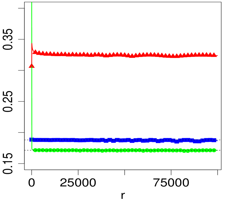
(a) $\lambda=0$

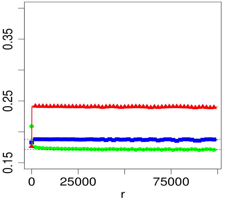
(b) $\lambda=2$

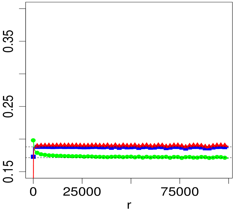
(c) $\lambda=4$

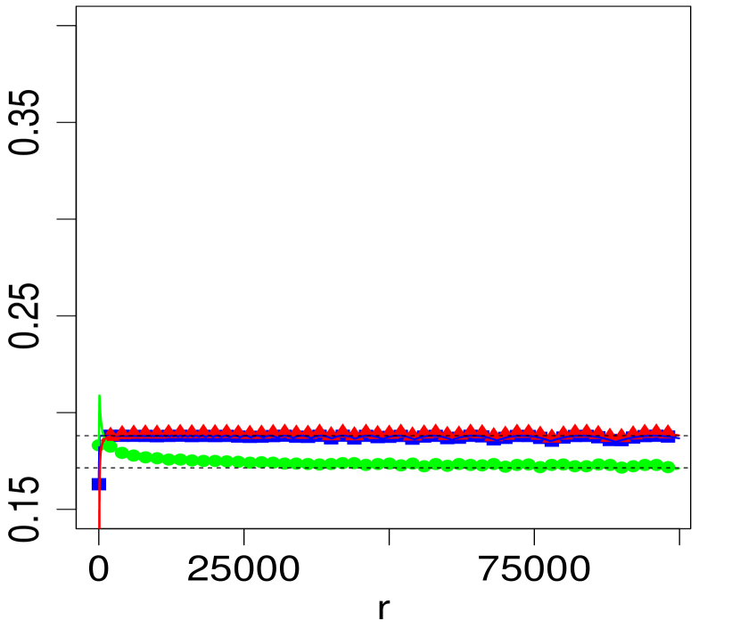
(d) $\lambda=6$

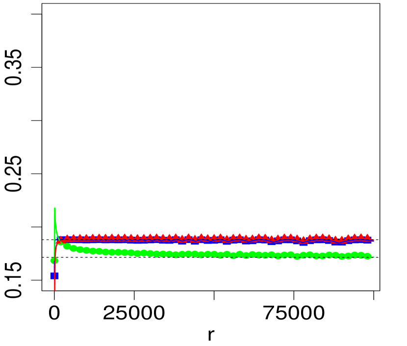
(e) $\lambda=8$

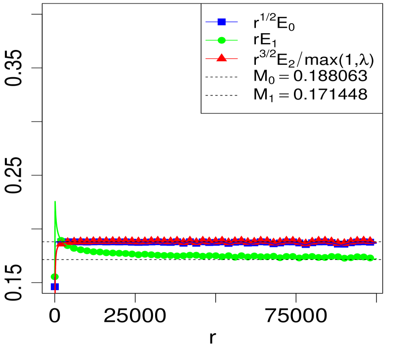
(f) $\lambda=10$

Figure 3.1: Numerical illustration of the asymptotic constants $M_{0}$, $M_{1}$ and $M_{2}$, for each $\lambda\in\{0,2,4,6,8,10\}$.

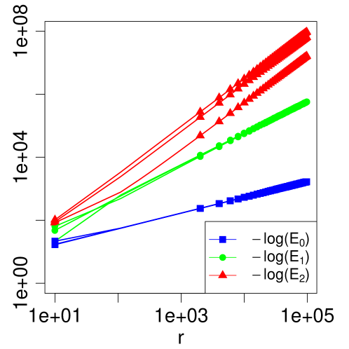
Figure 3.2: Log-log plot for the maximum absolute errors $E_{0}$, $E_{1}$ and $E_{2}$, as a function of $r$, for $\lambda=0$, $\lambda=2$ and $\lambda=10$.

4 Applications

4.1 Probability metrics upper bounds between chi-square and normal distributions

For our first application, we use Lemma 3.1 to compute an upper bound on the total variation between the probability measures induced by (1.1) and (1.3). Given the relation there is between the total variation and other probability metrics such as the Hellinger distance (see, e.g., Gibbs & Su, (2002, p.421)), we obtain upper bounds on other distance measures automatically.

Theorem 4.1 (Probability metrics bounds).

Let $r>0$ and $0\leq\lambda=\mathrm{o}(\sqrt{r})$. Let $\mathbb{P}_{r,\lambda}$ be the law of the $\chi_{r}^{2}(\lambda)$ distribution. Let $\mathbb{Q}_{r,\lambda}$ be the law of the $\mathrm{Normal}(r+\lambda,2(r+2\lambda))$ distribution. Then, as $r\to\infty$, we have

$$\mathrm{dist}\hskip 0.85358pt(\mathbb{P}_{r,\lambda},\mathbb{Q}_{r,\lambda})\leq\frac{C}{\sqrt{r}}\qquad\text{and}\qquad\mathcal{H}(\mathbb{P}_{r,\lambda},\mathbb{Q}_{r,\lambda})\leq\sqrt{\frac{2C}{\sqrt{r}}},$$ (4.1)

where $C>0$ is a universal constant, $\mathcal{H}(\cdot,\cdot)$ denotes the Hellinger distance, and $\mathrm{dist}\hskip 0.85358pt(\cdot,\cdot)$ can be replaced by any of the following probability metrics: Total variation, Kolmogorov (or Uniform) metric, Lévy metric, Discrepancy metric, Prokhorov metric.

Proof of Theorem 4.1.

Let $X\sim\mathbb{P}_{r,\lambda}$. By the comparison of the total variation norm $\|\cdot\|$ with the Hellinger distance on page 726 of Carter, (2002), we already know that

$$\|\mathbb{P}_{r,\lambda}-\mathbb{Q}_{r,\lambda}\|\leq\sqrt{2\,\mathbb{P}(X\in B_{r,\lambda}^{\hskip 0.56905ptc}(1/2))+\mathbb{E}\bigg{[}\log\left(\frac{{\rm d}\mathbb{P}_{r,\lambda}}{{\rm d}\mathbb{Q}_{r,\lambda}}(X)\right)\,\mathds{1}_{\{X\in B_{r,\lambda}(1/2)\}}\bigg{]}}.$$ (4.2)

Then, by applying a large deviation bound for the noncentral chi-square distribution (for example combine the Order $0$ approximation in Theorem 3.2 with a Mills ratio Gaussian tail inequality), we get, for $r$ large enough,

$$\mathbb{P}(X\in B_{r,\lambda}^{\hskip 0.56905ptc}(1/2)) \leq 100\,\exp\left(-\frac{1}{100}r^{1/3}\right).$$ (4.3)

By Lemma 3.1, we have

$$\mathbb{E}\bigg{[}\log\bigg{(}\frac{{\rm d}\mathbb{P}_{r,\lambda}}{{\rm d}\mathbb{Q}_{r,\lambda}}(X)\bigg{)}\,\mathds{1}_{\{X\in B_{r,\lambda}(1/2)\}}\bigg{]}$$ (4.4)

$$\quad=r^{-1/2}\cdot\mathbb{E}\left[\bigg{\{}\frac{\sqrt{2}}{3}\cdot\frac{(X-(r+\lambda))^{3}}{(2(r+2\lambda))^{3/2}}-\sqrt{2}\cdot\frac{(X-(r+\lambda))}{(2(r+2\lambda))^{1/2}}\bigg{\}}\,\mathds{1}_{\{X\in B_{r,\lambda}(1/2)\}}\right]$$

$$\quad\quad+r^{-1}\cdot\mathcal{O}\left(\frac{\mathbb{E}[(X-(r+\lambda))^{4}]}{(2(r+2\lambda))^{2}}+\frac{\mathbb{E}[(X-(r+\lambda))^{2}]}{2(r+2\lambda)}+1\right)$$

$$\quad\quad+\mathcal{O}(r^{-3/2}).$$

By Lemma B.1 and Corollary B.2, we get

$$\mathbb{E}\bigg{[}\log\bigg{(}\frac{{\rm d}\mathbb{P}_{r,\lambda}}{{\rm d}\mathbb{Q}_{r,\lambda}}(X)\bigg{)}\,\mathds{1}_{\{X\in B_{r,\lambda}(1/2)\}}\bigg{]}$$ (4.5)

$$\quad=r^{-1/2}\cdot(\mathbb{P}(X\in B_{r,\lambda}^{\hskip 0.56905ptc}(1/2)))^{1/2}+r^{-1}\cdot\mathcal{O}(1)+\mathcal{O}(r^{-3/2})$$

$$\quad=\mathcal{O}(r^{-1}).$$

This ends the proof. ∎

4.2 Asymptotics of the median

For our second application, we improve the lower bound for the median of the noncentral chi-square distribution found in Proposition 4.1 of Robert, (1990) (the upper bounds are comparable). The proof relies on the refined normal approximation in Theorem 3.2, a Taylor expansion for the c.d.f. of the standard normal distribution, and solving a quadratic equation involving the normalized (via $\delta_{\cdot}$) median.

Theorem 4.2.

Let $r>0$ and $0\leq\lambda=\mathrm{o}(\sqrt{r})$, and let $X\sim\chi_{r}^{2}(\lambda)$. Then, we have

$$\mathrm{Median}\hskip 0.85358pt(X)=r+\lambda-\frac{2}{3}+\mathcal{O}\left(\frac{1}{r^{1/2}}\right)+\mathcal{O}\left(\frac{1\vee\lambda}{r}\right),\quad\text{as }r\to\infty.$$ (4.6)

Proof of Theorem 4.2.

By definition, the median of the $\chi_{r}^{2}(\lambda)$ distribution is the point $a^{\star}>0$ that satisfies $S_{r,\lambda}(a^{\star})=1/2$. By the Order 1 approximation in Theorem 3.2, we want to find $a^{\star}$ such that

$$\left|\Psi\big{(}\delta_{a^{\star}-d_{1}}\big{)}-\frac{1}{2}\right|\leq\frac{M_{1}}{r}+\frac{C_{1}(1\vee\lambda)}{r^{3/2}}.$$ (4.7)

A Taylor expansion for $\Psi$ at $0$ yields

$$\Psi(x)=\frac{1}{2}-\frac{x}{\sqrt{2\pi}}+\mathcal{O}(x^{3}),\quad\text{as }x\to 0.$$ (4.8)

Equation (4.7) then becomes

$$\left|a^{\star}-d_{1}-(r+\lambda)+\mathcal{O}(r^{-1})\right|\leq\frac{\widetilde{M}_{1}}{r^{1/2}}+\frac{\widetilde{C}_{1}(1\vee\lambda)}{r},$$ (4.9)

for appropriate universal constants $\widetilde{M}_{1},\widetilde{C}_{1}>0$. The error $\mathcal{O}(r^{-1})$ in (4.9) does not depend on $\lambda$ because $\delta_{a^{\star}-d_{1}}=\mathcal{O}(r^{-1/2})$ by the a priori bounds we have from Proposition 4.1 in Robert, (1990). From (4.9) and the expression for $d_{1}$ (at $a=a^{\star}$) in (3.10), we deduce

$$\delta_{a^{\star}}=\frac{\frac{2}{3}(\delta_{a^{\star}}^{2}-1)}{\sqrt{2(r+2\lambda)}}+\mathcal{O}\left(\frac{1}{r}\right)+\mathcal{O}\left(\frac{1\vee\lambda}{r^{3/2}}\right).$$ (4.10)

This quadratic equation in the variable $\delta_{a^{\star}}$ yields the following two solutions (with the notation $\varepsilon_{r,\lambda}\vcentcolon=1/\sqrt{2(r+2\lambda)}$):

$$(\delta_{a^{\star}})_{1,2}=\frac{-1\pm\sqrt{1-4\cdot\frac{-2}{3}\varepsilon_{r,\lambda}\cdot\big{[}\frac{2}{3}\varepsilon_{r,\lambda}-\mathcal{O}\big{(}\frac{1}{r}\big{)}+\mathcal{O}\big{(}\frac{1\vee\lambda}{r^{3/2}}\big{)}\big{]}}}{2\cdot\frac{-2}{3}\varepsilon_{r,\lambda}}$$ (4.11)

Because of the a priori bounds on the median in Proposition 4.1 of Robert, (1990), the unique solution must be the one with the minus in (4.11). Therefore, the median $a^{\star}$ satisfies

$$a^{\star}-(r+\lambda)=\frac{1-\sqrt{1+\frac{16}{9}\varepsilon_{r,\lambda}^{2}+\mathcal{O}\big{(}\frac{1}{r^{3/2}}\big{)}+\mathcal{O}\big{(}\frac{1\vee\lambda}{r^{2}}\big{)}}}{\frac{4}{3}\varepsilon_{r,\lambda}^{2}}.$$ (4.12)

Using the Taylor expansion $\sqrt{1+y}=1+\frac{y}{2}+\mathcal{O}(y^{2}),~{}\text{as }y\to 0$, we have

$$a^{\star}-(r+\lambda)=-\frac{2}{3}+\mathcal{O}\left(\frac{1}{r^{1/2}}\right)+\mathcal{O}\left(\frac{1\vee\lambda}{r}\right).$$ (4.13)

This ends the proof. ∎

Remark 4.3.

It is possible to use the higher order approximations from Theorem 3.2 and apply the same logic in the proof of Theorem 4.2 to derive an expression for the median which is asymptotically more precise, but the algebra becomes much uglier. In particular, the degree of the polynomial equation to solve in (4.10) will increase.

Appendix A Proofs

Proof of Lemma 3.1.

By taking the logarithm in (1.1), we have

$$\log\big{(}f_{r,\lambda}(x)\big{)}=-\log 2-\frac{x+\lambda}{2}+\left(\frac{r}{2}-1\right)\log\left(\frac{x}{2}\right)+\log\sum_{j=0}^{\infty}\frac{(\lambda x/4)^{j}}{j!\,\Gamma(r/2+j)}.$$ (A.1)

Since

$$x=(r+\lambda)\,\left(1+\frac{\delta_{x}}{D_{r,\lambda}}\right),$$ (A.2)

we can rewrite (A.1) as

$$\log\big{(}f_{r,\lambda}(x)\big{)} =-\log 2-\frac{r+\lambda}{2}\left(1+\frac{\delta_{x}}{D_{r,\lambda}}\right)-\frac{\lambda}{2}+\left(\frac{r}{2}-1\right)\log\left(\frac{r+\lambda}{2}\right)$$ (A.3)

$$\quad+\left(\frac{r}{2}-1\right)\log\left(1+\frac{\delta_{x}}{D_{r,\lambda}}\right)-\log\Gamma\left(\frac{r}{2}\right)$$

$$\quad+\log\sum_{j=0}^{\infty}\frac{1}{j!}\left(\frac{\lambda}{2}\,\bigg{(}1+\frac{\delta_{x}}{D_{r,\lambda}}\bigg{)}\right)^{j}\,\frac{2^{-j}(r+\lambda)^{j}\Gamma(r/2)}{\Gamma(r/2+j)}.$$

Using the expansions

$$\left(\frac{r}{2}-1\right)\log\left(\frac{r+\lambda}{2}\right)=\left(\frac{r}{2}-1\right)\log\left(\frac{r}{2}\right)+\frac{\lambda}{2}-\frac{\lambda+\lambda^{2}/4}{r}+\mathcal{O}\left(\frac{1\vee\lambda^{3}}{r^{2}}\right),$$ (A.4)

and

$$\log\Gamma\left(\frac{r}{2}\right)=\left(\frac{r}{2}-\frac{1}{2}\right)\log\left(\frac{r}{2}\right)-\frac{r}{2}+\frac{1}{2}\log(2\pi)+\frac{1}{6r}+\mathcal{O}(r^{-3}),$$ (A.5)

(the first one is just a Taylor expansion for $r^{-1}$ at $0$, and the second one can be found, for example, in (Abramowitz & Stegun,, 1964, p.257)) we can rewrite (A.3) as

$$\log\big{(}f_{r,\lambda}(x)\big{)} =-\frac{1}{2}\log(2\pi\,2r)-\frac{r}{2}\,\frac{\delta_{x}}{D_{r,\lambda}}-\frac{\lambda}{2}\left(1+\frac{\delta_{x}}{D_{r,\lambda}}\right)$$ (A.6)

$$\quad+\left(\frac{r}{2}-1\right)\log\left(1+\frac{\delta_{x}}{D_{r,\lambda}}\right)-\frac{\frac{1}{6}+\lambda+\lambda^{2}/4}{r}+\mathcal{O}\left(\frac{1\vee\lambda^{3}}{r^{2}}\right)$$

$$\quad+\log\sum_{j=0}^{\infty}\frac{1}{j!}\left(\frac{\lambda}{2}\,\bigg{(}1+\frac{\delta_{x}}{D_{r,\lambda}}\bigg{)}\right)^{j}\,\frac{2^{-j}(r+\lambda)^{j}\Gamma(r/2)}{\Gamma(r/2+j)}.$$

Now,

$$\frac{2^{-j}(r+\lambda)^{j}\Gamma(r/2)}{\Gamma(r/2+j)} =1+\frac{j(\lambda+1)-j^{2}}{r}$$ (A.7)

$$\quad+\mathcal{O}\bigg{(}\frac{(1\vee\lambda^{2})(j+j^{2})+(1\vee\lambda)j^{3}+j^{4}}{r^{2}}\bigg{)},$$

and, for any $a\in\mathbb{R}$,

$$\log\left(\sum_{j=0}^{\infty}\frac{a^{j}}{j!}\,\left\{1+\frac{j(\lambda+1)-j^{2}}{r}+\mathcal{O}\bigg{(}\frac{(1\vee\lambda^{2})(j+j^{2})+(1\vee\lambda)j^{3}+j^{4}}{r^{2}}\bigg{)}\right\}\right)$$ (A.8)

$$=a+\log\left(1+\frac{a(\lambda-a)}{r}+\mathcal{O}\left(\frac{|a|}{r^{2}}\cdot\left\{\begin{array}[]{l}(1\vee\lambda^{2})(1+|a|)\\ +(1\vee\lambda)(1+|a|^{2})+(1+|a|^{3})\end{array}\right\}\right)\right),$$

so if we take

$$a=\frac{\lambda}{2}\,\bigg{(}1+\frac{\delta_{x}}{D_{r,\lambda}}\bigg{)},$$ (A.9)

we can rewrite (A.6) as

$$\log\big{(}f_{r,\lambda}(x)\big{)} =-\frac{1}{2}\log(2\pi\,2r)-\frac{r}{2}\,\frac{\delta_{x}}{D_{r,\lambda}}$$ (A.10)

$$\quad+\left(\frac{r}{2}-1\right)\log\left(1+\frac{\delta_{x}}{D_{r,\lambda}}\right)-\frac{\frac{1}{6}+\lambda+\lambda^{2}/4}{r}+\mathcal{O}\left(\frac{1\vee\lambda^{3}}{r^{2}}\right)$$

$$\quad+\log\left(1+\frac{\lambda}{2r}\,\left(1+\frac{\delta_{x}}{D_{r,\lambda}}\right)\left[\lambda-\frac{\lambda}{2}\,\left(1+\frac{\delta_{x}}{D_{r,\lambda}}\right)\right]+\mathcal{O}\left(\frac{1\vee\lambda^{4}}{r^{2}}\right)\right).$$

Using the Taylor expansion

$$\log(1+y)=y-\frac{y^{2}}{2}+\frac{y^{3}}{3}-\frac{y^{4}}{4}+\frac{y^{5}}{5}+\mathcal{O}_{\eta}(y^{6}),$$ (A.11)

valid for $|y|\leq\eta<1$, we have

$$\log\big{(}f_{r,\lambda}(x)\big{)} =-\frac{1}{2}\log(2\pi\,2r)-\frac{r}{2}\,\frac{\delta_{x}}{D_{r,\lambda}}-\frac{\frac{1}{6}+\lambda}{r}+\mathcal{O}\left(\frac{(1\vee\lambda^{4})+\lambda^{2}|\delta_{x}|^{2}}{r^{2}}\right)$$

$$\quad+\left(\frac{r}{2}-1\right)\,\left\{\begin{array}[]{l}\frac{\delta_{x}}{D_{r,\lambda}}-\frac{1}{2}\big{(}\frac{\delta_{x}}{D_{r,\lambda}}\big{)}^{2}+\frac{1}{3}\big{(}\frac{\delta_{x}}{D_{r,\lambda}}\big{)}^{3}-\frac{1}{4}\big{(}\frac{\delta_{x}}{D_{r,\lambda}}\big{)}^{4}\\ +\frac{1}{5}\big{(}\frac{\delta_{x}}{D_{r,\lambda}}\big{)}^{5}+\mathcal{O}_{\eta}\left(\frac{1+|\delta_{x}|^{6}}{r^{3}}\right)\end{array}\right\}$$ (A.14)

$$=-\frac{1}{2}\log(2\pi\,2r)-\frac{\frac{1}{6}+\lambda}{r}+\mathcal{O}\left(\frac{(1\vee\lambda^{4})+\lambda^{2}|\delta_{x}|^{2}}{r^{2}}\right)$$

$$\quad-\frac{\sqrt{2(r+2\lambda)}}{(r+\lambda)}\delta_{x}-\frac{(r-2)(r+2\lambda)}{2(r+\lambda)^{2}}\delta_{x}^{2}+\frac{(r-2)2^{1/2}(r+2\lambda)^{3/2}}{3(r+\lambda)^{3}}\delta_{x}^{3}$$

$$\quad-\frac{(r-2)(r+2\lambda)^{2}}{2(r+\lambda)^{4}}\delta_{x}^{4}+\frac{(r-2)2^{3/2}(r+2\lambda)^{5/2}}{5(r+\lambda)^{5}}\delta_{x}^{5}.$$ (A.15)

Since

$$-\frac{\sqrt{2(r+2\lambda)}}{(r+\lambda)} =-\frac{\sqrt{2}}{r^{1/2}}+\mathcal{O}\left(\frac{1\vee\lambda^{2}}{r^{5/2}}\right),$$ (A.16)

$$-\frac{(r-2)(r+2\lambda)}{2(r+\lambda)^{2}} =-\frac{1}{2}+\frac{1}{r}+\mathcal{O}\left(\frac{1\vee\lambda^{2}}{r^{2}}\right),$$

$$\frac{(r-2)2^{1/2}(r+2\lambda)^{3/2}}{3(r+\lambda)^{3}} =\frac{\sqrt{2}/3}{r^{1/2}}-\frac{2^{3/2}/3}{r^{3/2}}+\mathcal{O}\left(\frac{1\vee\lambda^{2}}{r^{5/2}}\right),$$

$$-\frac{(r-2)(r+2\lambda)^{2}}{2(r+\lambda)^{4}} =-\frac{1}{2r}+\mathcal{O}\left(\frac{1}{r^{2}}\right),$$

$$\frac{(r-2)2^{3/2}(r+2\lambda)^{5/2}}{5(r+\lambda)^{5}} =\frac{2^{3/2}/5}{r^{3/2}}+\mathcal{O}\left(\frac{1}{r^{5/2}}\right),$$

and

$$-\frac{1}{2}\log(2\pi\,2r)=-\frac{1}{2}\log(2\pi\,2(r+2\lambda))+\frac{\lambda}{r}+\mathcal{O}\left(\frac{1\vee\lambda^{2}}{r^{2}}\right),$$ (A.17)

we can rewrite (A) as

$$\log\bigg{(}\frac{f_{r,\lambda}(x)}{\frac{1}{\sqrt{2(r+2\lambda)}}\phi(\delta_{x})}\bigg{)} =r^{-1/2}\,\bigg{\{}\frac{\sqrt{2}}{3}\,\delta_{x}^{3}-\sqrt{2}\,\delta_{x}\bigg{\}}+r^{-1}\,\bigg{\{}-\frac{1}{2}\,\delta_{x}^{4}+\delta_{x}^{2}-\frac{1}{6}\bigg{\}}$$

$$\quad+r^{-3/2}\,\bigg{\{}\frac{2^{3/2}}{5}\,\delta_{x}^{5}-\frac{2^{3/2}}{3}\,\delta_{x}^{3}\bigg{\}}+\mathcal{O}\left(\frac{(1\vee\lambda^{4})+\lambda^{2}|\delta_{x}|^{2}}{r^{2}}\right),$$ (A.18)

which proves (3.1). To obtain (3.1) and conclude the proof, we take the exponential on both sides of the last equation and we expand the right-hand side with

$$e^{y}=1+y+\frac{y^{2}}{2}+\frac{y^{3}}{6}+\mathcal{O}(e^{\widetilde{\eta}}y^{4}),\quad-\infty<y\leq\widetilde{\eta}.$$ (A.19)

For $r$ large enough and uniformly for $x\in B_{r,\lambda}(\eta)$, the right-hand side of (A) is $\mathcal{O}_{\lambda}(1)$. When this bound is taken as $y$ in (A.19), it explains the error in (3.1). ∎

Proof of Theorem 3.2.

Let

$$c=d_{1}+\frac{d_{2}}{\sqrt{r}}+\frac{d_{3}}{r},$$ (A.20)

where $d_{1},d_{2},d_{3}\in\mathbb{R}$ are to be chosen later, then we have the Taylor expansion

$$\int_{\delta_{a-c}}^{\delta_{a}}\phi(y){\rm d}y =\phi(\delta_{a})\int_{\delta_{a-c}}^{\delta_{a}}{\rm d}y+\phi^{\prime}(\delta_{a})\int_{\delta_{a-c}}^{\delta_{a}}(y-\delta_{a}){\rm d}y+\frac{\phi^{\prime\prime}(\delta_{a})}{2}\int_{\delta_{a-c}}^{\delta_{a}}(y-\delta_{a})^{2}{\rm d}y$$ (A.21)

$$\quad+\mathcal{O}\left(\frac{\phi^{\prime\prime\prime}(\delta_{a})}{6}\int_{\delta_{a-c}}^{\delta_{a}}(y-\delta_{a})^{3}{\rm d}y\right)$$

$$=\phi(\delta_{a})\,\left\{\begin{array}[]{l}\frac{c}{\sqrt{2(r+2\lambda)}}+\frac{c^{2}\,\delta_{a}}{4(r+2\lambda)}\\[5.69054pt] +\frac{c^{3}(\delta_{a}^{2}-1)}{6\cdot 2^{3/2}(r+2\lambda)^{3/2}}+\mathcal{O}\big{(}\frac{1+|\delta_{a}|^{3}}{r^{2}}\big{)}\end{array}\right\}$$

$$=\phi(\delta_{a})\,\left\{\begin{array}[]{l}r^{-1/2}\,\frac{1}{\sqrt{2}}\,d_{1}+r^{-1}\,\big{(}\frac{\delta_{a}}{4}\,d_{1}^{2}+\frac{1}{\sqrt{2}}\,d_{2}\big{)}\\[2.84526pt] r^{-3/2}\,\bigg{(}\begin{array}[]{l}\frac{(\delta_{a}^{2}-1)}{12\sqrt{2}}\,d_{1}^{3}-\frac{\lambda}{\sqrt{2}}\,d_{1}\\[2.84526pt] +\frac{\delta_{a}}{2}\,d_{1}d_{2}+\frac{1}{\sqrt{2}}\,d_{3}\end{array}\bigg{)}+\mathcal{O}\big{(}\frac{1+|\delta_{a}|^{3}}{r^{2}}\big{)}\end{array}\right\}$$

We also have the straightforward large deviation bounds

$$\int_{[a,\infty)\cap B_{r,\lambda}^{\hskip 0.56905ptc}(1/2)}f_{r,\lambda}(x){\rm d}x=\mathcal{O}(e^{-\beta r^{1/3}}),$$ (A.22)

$$\int_{[a,\infty)\cap B_{r,\lambda}^{\hskip 0.56905ptc}(1/2)}\phi(y){\rm d}y=\mathcal{O}(e^{-\beta r^{1/3}}),$$

where $\beta=\beta(\lambda)>0$ is a small enough constant, and the local approximation in Lemma 3.1 yields

$$\int_{a}^{\infty}f_{r,\lambda}(x){\rm d}x-\int_{\delta_{a}}^{\infty}\phi(y){\rm d}y =r^{-1/2}\bigg{\{}\frac{\sqrt{2}}{3}\Psi_{3}(\delta_{a})-\sqrt{2}\Psi_{1}(\delta_{a})\bigg{\}}$$ (A.23)

$$\quad+r^{-1}\left\{\frac{1}{9}\Psi_{6}(\delta_{a})-\frac{7}{6}\Psi_{4}(\delta_{a})+2\Psi_{2}(\delta_{a})-\frac{1}{6}\Psi(\delta_{a})\right\}$$

$$\quad+r^{-3/2}\left\{\begin{array}[]{l}\frac{\sqrt{2}}{81}\Psi_{9}(\delta_{a})-\frac{5}{9\sqrt{2}}\Psi_{7}(\delta_{a})+\frac{47}{15\sqrt{2}}\Psi_{5}(\delta_{a})\\[4.2679pt] -\frac{37}{9\sqrt{2}}\Psi_{3}(\delta_{a})+\frac{1}{3\sqrt{2}}\Psi_{1}(\delta_{a})\end{array}\right\}$$

$$\quad+\mathcal{O}\left(\frac{1\vee\lambda^{4}}{r^{2}}\right),$$

where $\Psi_{k}(\delta_{a})\vcentcolon=\int_{\delta_{a}}y^{k}\phi(y){\rm d}y$. Now, using the fact that

$$\Psi_{9}(\delta_{a})=(384+192\delta_{a}^{2}+48\delta_{a}^{4}+8\delta_{a}^{6}+\delta_{a}^{8})\phi(\delta_{a}),$$ (A.24)

$$\Psi_{7}(\delta_{a})=(48+24\delta_{a}^{2}+6\delta_{a}^{4}+\delta_{a}^{6})\phi(\delta_{a}),$$

$$\Psi_{6}(\delta_{a})=(15\delta_{a}+5\delta_{a}^{3}+\delta_{a}^{5})\phi(\delta_{a})+15\Psi(\delta_{a}),$$

$$\Psi_{5}(\delta_{a})=(8+4\delta_{a}^{2}+\delta_{a}^{4})\phi(\delta_{a}),$$

$$\Psi_{4}(\delta_{a})=(3\delta_{a}+\delta_{a}^{3})\phi(\delta_{a})+3\Psi(\delta_{a}),$$

$$\Psi_{3}(\delta_{a})=(2+\delta_{a}^{2})\phi(\delta_{a}),$$

$$\Psi_{2}(\delta_{a})=\delta_{a}\phi(\delta_{a})+\Psi(\delta_{a}),$$

$$\Psi_{1}(\delta_{a})=\phi(\delta_{a}),$$

where $\Psi$ denotes the survival function of the standard normal distribution, Equations (A.21), (A.22) and (A.23) together yield

$$\int_{a}^{\infty}f_{r,\lambda}(x){\rm d}x-\int_{\delta_{a-c}}^{\infty}\phi(y){\rm d}y$$ (A.25)

$$\qquad=r^{-1/2}\bigg{\{}\frac{\sqrt{2}}{3}(\delta_{a}^{2}-1)-\frac{1}{\sqrt{2}}\,d_{1}\bigg{\}}\,\phi(\delta_{a})$$

$$\qquad\quad+r^{-1}\left\{\frac{\delta_{a}}{18}\left(2\delta_{a}^{4}-11\delta_{a}^{2}+3\right)-\left(\frac{\delta_{a}}{4}\,d_{1}^{2}+\frac{1}{\sqrt{2}}\,d_{2}\right)\right\}\,\phi(\delta_{a})$$

$$\qquad\quad+r^{-3/2}\left\{\begin{array}[]{l}\frac{\sqrt{2}}{81}\delta_{a}^{8}-\frac{29}{81\sqrt{2}}\delta_{a}^{6}+\frac{133}{135\sqrt{2}}\delta_{a}^{4}-\frac{23}{135\sqrt{2}}\delta_{a}^{2}-\frac{1}{135\sqrt{2}}\\[2.84526pt] -\left(\frac{(\delta_{a}^{2}-1)}{12\sqrt{2}}\,d_{1}^{3}-\frac{\lambda}{\sqrt{2}}\,d_{1}+\frac{\delta_{a}}{2}\,d_{1}d_{2}+\frac{1}{\sqrt{2}}\,d_{3}\right)\end{array}\right\}\,\phi(\delta_{a})$$

$$\qquad\quad+\mathcal{O}\left(\frac{1\vee\lambda^{4}}{r^{2}}\right).$$

If we select $d_{1}=d_{2}=d_{3}=0$, then

$$\max_{a\in\mathbb{R}}\left|\int_{a}^{\infty}f_{r,\lambda}(x){\rm d}x-\int_{\delta_{a-c}}^{\infty}\phi(y){\rm d}y\right|$$ (A.26)

$$\quad\leq r^{-1/2}\,\max_{a\in\mathbb{R}}\frac{\sqrt{2}}{3}|\delta_{a}^{2}-1|\phi(\delta_{a})+\mathcal{O}(r^{-1}).$$

Since $\max_{y\in\mathbb{R}}\frac{\sqrt{2}}{3}|y^{2}-1|\phi(y)=\frac{1}{\sqrt{9\pi}}$, this proves (3.6). If we select $d_{1}=\frac{2}{3}(\delta_{a}^{2}-1)$ and $d_{2}=d_{3}=0$ to cancel the first brace in (A.25), then

$$\max_{a\in\mathbb{R}}\left|\int_{a}^{\infty}f_{r,\lambda}(x){\rm d}x-\int_{\delta_{a-c}}^{\infty}\phi(y){\rm d}y\right|$$ (A.27)

$$\quad\leq r^{-1}\,\max_{a\in\mathbb{R}}\frac{1}{18}|7\delta_{a}^{3}-\delta_{a}|\phi(\delta_{a})+\mathcal{O}\left(\frac{1\vee\lambda}{r^{3/2}}\right),$$

which proves (3.7). If we select $d_{1}=\frac{2}{3}(\delta_{a}^{2}-1)$, $d_{2}=\frac{1}{9\sqrt{2}}(\delta_{a}-7\delta_{a}^{3})$ and $d_{3}=0$ to cancel the first two braces in (A.25), then

$$\max_{a\in\mathbb{R}}\left|\int_{a}^{\infty}f_{r,\lambda}(x){\rm d}x-\int_{\delta_{a-c}}^{\infty}\phi(y){\rm d}y\right|$$ (A.28)

$$\quad\leq r^{-3/2}\,\max_{a\in\mathbb{R}}\frac{1}{405\sqrt{2}}\left|219\delta_{a}^{4}+(270\lambda-14)\delta_{a}^{2}-(270\lambda+13)\right|\phi(\delta_{a})$$

$$\quad\quad+\mathcal{O}\left(\frac{1\vee\lambda^{4}}{r^{2}}\right),$$

which proves (3.8). If we select $d_{1}=\frac{2}{3}(\delta_{a}^{2}-1)$, $d_{2}=\frac{1}{9\sqrt{2}}(\delta_{a}-7\delta_{a}^{3})$ and $d_{3}=\frac{1}{405}\big{(}219\delta_{a}^{4}+(270\lambda-14)\delta_{a}^{2}-(270\lambda+13)\big{)}$ to cancel the three braces in (A.25), then

$$\max_{a\in\mathbb{R}}\left|\int_{a}^{\infty}f_{r,\lambda}(x){\rm d}x-\int_{\delta_{a-c}}^{\infty}\phi(y){\rm d}y\right|=\mathcal{O}\left(\frac{1\vee\lambda^{4}}{r^{2}}\right),$$ (A.29)

which proves (3.9). This ends the proof. ∎

Appendix B Moments of the central and noncentral chi-square distribution

In the lemma below, we prove a general formula for the central moments of the central and noncentral chi-square distribution, and we evaluate the first, second, third, fourth and sixth central moments explicitly. This lemma is used to estimate the $\asymp r^{-1}$ errors in (4.4) of the proof of Theorem 4.1. It is also a preliminary result for the proof of Corollary B.2 below, where the central moments are estimated on various events.

Lemma B.1 (Central moments).

Let $X\sim\chi_{r}^{2}(\lambda)$ for some $r>0$ and $\lambda\geq 0$. We have

$$\mathbb{E}[(X-(r+\lambda))]=0,$$ (B.1)

$$\mathbb{E}[(X-(r+\lambda))^{2}]=2\,(r+2\lambda),$$

$$\mathbb{E}[(X-(r+\lambda))^{3}]=8\,(r+3\lambda),$$

$$\mathbb{E}[(X-(r+\lambda))^{4}]=12\,(r^{2}+4r(1+\lambda)+4\lambda(4+\lambda)),$$

$$\mathbb{E}[(X-(r+\lambda))^{6}]=40\left(\begin{array}[]{l}3r^{3}+2r^{2}(26+9\lambda)+12r(8+26\lambda+3\lambda^{2})\\ +24\lambda(24+18\lambda+\lambda^{2})\end{array}\right).$$

Proof of Lemma B.1.

One way to compute these central moments would be to apply the recurrence formula developed in Withers & Nadarajah, (2007). An other method consists in differentiating the moment-generating function

$$\mathbb{E}[e^{tX}]=(1-2t)^{-r/2}\exp\bigg{(}\frac{\lambda t}{1-2t}\bigg{)},\quad t<1/2,$$ (B.2)

in order to find $\mathbb{E}[X^{i}],\,i\in\mathbb{N},$ and then use the binomial formula:

$$\mathbb{E}[(X-(r+\lambda))^{n}]=\sum_{i=0}^{n}\binom{n}{i}\mathbb{E}[X^{i}]\,(-1)^{n-i}(r+\lambda)^{n-i},\quad n\in\mathbb{N}.$$ (B.3)

Using the latter approach with Mathematica give us the result. ∎

We can also estimate the moments of Lemma B.1 on various events. The corollary below is used to estimate the $\asymp r^{-1/2}$ errors in (4.4) of the proof of Theorem 4.1.

Corollary B.2 (Central moments on various events).

Let $X\sim\chi_{r}^{2}(\lambda)$ for some $r>0$ and $0\leq\lambda\leq r$, and let $A\in\mathscr{B}(\mathbb{R})$ be a Borel set. Then,

$$\big{|}\mathbb{E}[(X-(r+\lambda))\,\mathds{1}_{\{X\in A\}}]\big{|}\leq 6^{1/2}\,r^{1/2}\,(\mathbb{P}(X\in A^{c}))^{1/2},$$ (B.4)

$$\big{|}\mathbb{E}[(X-(r+\lambda))^{2}\,\mathds{1}_{\{X\in A\}}]-2\,(r+2\lambda)\big{|}\leq 348^{1/2}\,r\,(\mathbb{P}(X\in A^{c}))^{1/2},$$

$$\big{|}\mathbb{E}[(X-(r+\lambda))^{3}\,\mathds{1}_{\{X\in A\}}]-8\,(r+3\lambda)\big{|}\leq 61960^{1/2}\,r^{3/2}\,(\mathbb{P}(X\in A^{c}))^{1/2}.$$

Proof of Corollary B.2.

Note that (B.1) implies

$$\mathbb{E}[(X-(r+\lambda))^{2}]=6\,r,$$ (B.5)

$$\mathbb{E}[(X-(r+\lambda))^{4}]\leq 348\,r^{2},$$

$$\mathbb{E}[(X-(r+\lambda))^{6}]\leq 61960\,r^{3}.$$

By (B.1), we also have

$$\big{|}\mathbb{E}[(X-(r+\lambda))\,\mathds{1}_{\{X\in A\}}]\big{|}=\big{|}\mathbb{E}[(X-(r+\lambda))\,\mathds{1}_{\{X\in A^{c}\}}]\big{|},$$ (B.6)

$$\big{|}\mathbb{E}[(X-(r+\lambda))^{2}\,\mathds{1}_{\{X\in A\}}]-2\,(r+2\lambda)\big{|}=\big{|}\mathbb{E}[(X-(r+\lambda))^{2}\,\mathds{1}_{\{X\in A^{c}\}}]\big{|},$$

$$\big{|}\mathbb{E}[(X-(r+\lambda))^{3}\,\mathds{1}_{\{X\in A\}}]-8\,(r+3\lambda)\big{|}=\big{|}\mathbb{E}[(X-(r+\lambda))^{3}\,\mathds{1}_{\{X\in A^{c}\}}]\big{|}.$$

We get (B.4) by applying the Cauchy-Schwarz inequality and bounding using (B.5). ∎

References

- Abdel-Aty, (1954) Abdel-Aty, S. H. 1954. Approximate formulae for the percentage points and the probability integral of the non-central distribution. Biometrika, 41(3/4), 538–540. doi:10.2307/2332731.
- Abramowitz & Stegun, (1964) Abramowitz, M., & Stegun, I. A. 1964. Handbook of mathematical functions with formulas, graphs, and mathematical tables. National Bureau of Standards Applied Mathematics Series, vol. 55. For sale by the Superintendent of Documents, U.S. Government Printing Office, Washington, D.C. MR0167642.
- Anderson, (1981) Anderson, D. A. 1981. Maximum likelihood estimation in the noncentral chi distribution with unknown scale parameter. Sankhyā Ser. B, 43(1), 58–67. MR661020.
- Ashour & Abdel-Samad, (1990) Ashour, S. K., & Abdel-Samad, A. I. 1990. On the computation of noncentral chi-square distribution function. Comm. Statist. Simulation Comput., 19(4), 1279–1291. MR1097704.
- Baricz et al., (2021) Baricz, A., Jankov, M. D., & Pogány, T. K. 2021. Approximation of CDF of non-central chi-square distribution by mean-value theorems for integrals. Mathematics, 9(2). doi:10.3390/math9020129.
- Berkson, (1946) Berkson, J. 1946. Approximation of chi-square by “probits” and by “logits.”. J. Amer. Statist. Assoc., 41, 70–74. MR15734.
- Bock & Govindarajulu, (1988) Bock, M. E., & Govindarajulu, Z. 1988. A note on the noncentral chi-square distribution. Statist. Probab. Lett., 7(2), 127–129. MR980908.
- Canal, (2005) Canal, L. 2005. A normal approximation for the chi-square distribution. Comput. Statist. Data Anal., 48(4), 803–808. MR2133578.
- Carter, (2002) Carter, A. V. 2002. Deficiency distance between multinomial and multivariate normal experiments. Ann. Statist., 30(3), 708–730. MR1922539.
- Chattamvelli & Shanmugam, (1995) Chattamvelli, R., & Shanmugam, R. 1995. Efficient computation of the noncentral distribution. Commun. Stat. - Simul. Comput., 24(3), 675–689. doi:10.1080/03610919508813266.
- Chou et al., (1984) Chou, Y.-M., Arthur, K. H., Rosenstein, R. B., & Owen, D. B. 1984. New representations of the noncentral chi-square density and cumulative. Comm. Statist. A—Theory Methods, 13(21), 2673–2678. MR759243.
- Chow, (1987) Chow, M. S. 1987. A complete class theorem for estimating a noncentrality parameter. Ann. Statist., 15(2), 800–804. MR888440.
- Cressie, (1978) Cressie, N. 1978. A finely tuned continuity correction. Ann. Inst. Statist. Math., 30(3), 435–442. MR538319.
- Cressie & Hawkins, (1980) Cressie, N., & Hawkins, D. M. 1980. Robust estimation of the variogram. I. J. Internat. Assoc. Math. Geol., 12(2), 115–125. MR595404.
- de Waal, (1974) de Waal, D. J. 1974. Bayes estimate of the noncentrality parameter in multivariate analysis. Comm. Statist., 3, 73–79. MR331611.
- Ding, (1992) Ding, C. G. 1992. Algorithm AS 275: Computing the non-central distribution function. J. R. Stat. Soc. C-Appl., 41(2), 478–482. doi:10.2307/2347584.
- Dinges, (1989) Dinges, H. 1989. Special cases of second order Wiener germ approximations. Probab. Theory Related Fields, 83(1-2), 5–57. MR1012493.
- Esseen, (1945) Esseen, C.-G. 1945. Fourier analysis of distribution functions. A mathematical study of the Laplace-Gaussian law. Acta Math., 77, 1–125. MR14626.
- Fisher, (1922) Fisher, R. A. 1922. On the interpretation of from contingency tables, and the calculation of P. J. R. Stat. Soc., 85(1), 87–94. doi:10.2307/2340521.
- Fisher, (1928) Fisher, R. A. 1928. Statistical methods for research workers. Second edition.
- Fraser et al., (1998) Fraser, D. A. S., Wong, A. C. M., & Wu, J. 1998. An approximation for the noncentral chi-squared distribution. Comm. Statist. Simulation Comput., 27(2), 275–287. MR1625949.
- Gaunt & Reinert, (2021) Gaunt, R. E., & Reinert, G. 2021. Bounds for the chi-square approximation of Friedman’s statistic by Stein’s method. Preprint, 1–38. arXiv:2111.00949.
- Gaunt et al., (2017) Gaunt, R. E., Pickett, A. M., & Reinert, G. 2017. Chi-square approximation by Stein’s method with application to Pearson’s statistic. Ann. Appl. Probab., 27(2), 720–756. MR3655852.
- Germond & Hastings, (1944) Germond, H. H., & Hastings, C. 1944. Scatter bombing of a circular target. Technical Report - Bombing Researcg Group - Columbia University, 95 pp. [URL] https://www.informs.org/content/download/302982/2898490/file/BombDIspersalANalysis.pdf.
- Gibbs & Su, (2002) Gibbs, A. L., & Su, F. E. 2002. On choosing and bounding probability metrics. Int. Stat. Rev., 70(3), 419–435. doi:10.2307/1403865.
- Govindarajulu, (1965) Govindarajulu, Z. 1965. Normal approximations to the classical discrete distributions. Sankhyā Ser. A, 27, 143–172. MR207011.
- Gray et al., (1969) Gray, H. L., Thompson, R. W., & McWilliams, G. V. 1969. A new approximation for the chi-square integral. Math. Comp., 23, 85–89. MR238470.
- Hawkins & Wixley, (1986) Hawkins, D. M., & Wixley, R. A. J. 1986. A note on the transformation of chi-squared variables to normality. Amer. Statist., 40(4), 296–298. doi:10.2307/2684608.
- Horgan & Murphy, (2013) Horgan, D., & Murphy, C. C. 2013. On the convergence of the chi square and noncentral chi square distributions to the normal distribution. IEEE Commun. Lett., 17(12), 2233–2236. doi:10.1109/LCOMM.2013.111113.131879.
- Johnson, (1959) Johnson, N. L. 1959. On an extension of the connexion between Poisson and distributions. Biometrika, 46, 352–363. MR109379.
- Johnson et al., (1995) Johnson, N. L., Kotz, S., & Balakrishnan, N. 1995. Continuous univariate distributions. Vol. 2. Second edn. Wiley Series in Probability and Mathematical Statistics: Applied Probability and Statistics. John Wiley & Sons, Inc., New York. MR1326603.
- Johnstone, (2001a) Johnstone, I. 2001a. Thresholding for weighted . Statist. Sinica, 11(3), 691–704. MR1863157.
- Johnstone, (2001b) Johnstone, I. M. 2001b. Chi-square oracle inequalities. Pages 399–418 of: State of the art in probability and statistics (Leiden, 1999). IMS Lecture Notes Monogr. Ser., vol. 36. Inst. Math. Statist., Beachwood, OH. MR1836572.
- Kubokawa et al., (1993) Kubokawa, T., Robert, C. P., & Saleh, A. K. Md. E. 1993. Estimation of noncentrality parameters. Canad. J. Statist., 21(1), 45–57. MR1221856.
- Kubokawa et al., (2017) Kubokawa, T., Marchand, É., & Strawderman, W. E. 2017. A unified approach to estimation of noncentrality parameters, the multiple correlation coefficient, and mixture models. Math. Methods Statist., 26(2), 134–148. MR3667406.
- Liu et al., (2009) Liu, H., Tang, Y., & Zhang, H. H. 2009. A new chi-square approximation to the distribution of non-negative definite quadratic forms in non-central normal variables. Comput. Statist. Data Anal., 53(4), 853–856. MR2657050.
- Maširević, (2017) Maširević, D. J. 2017. On new formulas for the cumulative distribution function of the noncentral chi-square distribution. Mediterr. J. Math., 14(2), Paper No. 66, 13 pp. MR3619428.
- Merrington, (1941) Merrington, M. 1941. Numerical approximations to the percentage points of the distribution. Biometrika, 32, 200–202. MR5588.
- Neff & Strawderman, (1976) Neff, N., & Strawderman, W. E. 1976. Further remarks on estimating the parameter of a noncentral chi-square distribution. Comm. Statist.–Theory Methods, A5(1), 65–76. MR0397966.
- Okagbue et al., (2017) Okagbue, H. I., Adamu, M. O., & Anake, T. A. 2017. Quantile approximation of the chi-square distribution using the quantile mechanics. In: Proceedings of the World Congress on Engineering and Computer Science, vol. 1. WCECS 2017, October 25-27, 2017, San Francisco, USA. http://eprints.covenantuniversity.edu.ng/9668/1/WCECS2017_pp477-483.pdf.
- Ouimet, (2021a) Ouimet, F. 2021a. On the Le Cam distance between Poisson and Gaussian experiments and the asymptotic properties of Szasz estimators. J. Math. Anal. Appl., 499(1), Paper No. 125033, 18 pp. MR4213687.
- Ouimet, (2021b) Ouimet, F. 2021b. A precise local limit theorem for the multinomial distribution and some applications. J. Statist. Plann. Inference, 215, 218–233. MR4249129.
- Ouimet, (2021c) Ouimet, F. 2021c. A refined continuity correction for the negative binomial distribution and asymptotics of the median. Preprint, 1–18. arXiv:2103.08846.
- Ouimet, (2022a) Ouimet, F. 2022a. An improvement of Tusnády’s inequality in the bulk. Adv. in Appl. Math., 133, Paper No. 102270, 24 pp. MR4340237.
- Ouimet, (2022b) Ouimet, F. 2022b. A multivariate normal approximation for the Dirichlet density and some applications. Stat, 11(1), Paper No. e410, 13 pp. MR4394974.
- Ouimet, (2022c) Ouimet, F. 2022c. On the Le Cam distance between multivariate hypergeometric and multivariate normal experiments. Results Math., 77(1), Paper No. 47, 11 pp. MR4361955.
- Ouimet, (2022d) Ouimet, F. 2022d. A symmetric matrix-variate normal local approximation for the Wishart distribution and some applications. J. Multivariate Anal., 189, Paper No. 104923, 17 pp. MR4358612.
- Patnaik, (1949) Patnaik, P. B. 1949. The non-central and -distributions and their applications. Biometrika, 36, 202–232. MR34564.
- Pearson, (1959) Pearson, E. S. 1959. Note on an approximation to the distribution of non-central . Biometrika, 46, 364. MR109380.
- Penev & Raykov, (2000) Penev, S., & Raykov, T. 2000. A Wiener Germ approximation of the noncentral chi square distribution and of its quantiles. Comput. Stat., 15, 219–228. doi:10.1007/s001800000029.
- Perlman & Rasmussen, (1975) Perlman, M. D., & Rasmussen, U. A. 1975. Some remarks on estimating a noncentrality parameter. Comm. Statist., 4, 455–468. MR378217.
- Robert, (1990) Robert, C. 1990. On some accurate bounds for the quantiles of a noncentral chi squared distribution. Statist. Probab. Lett., 10(2), 101–106. MR1072495.
- Robertson, (1969) Robertson, G. H. 1969. Computation of the noncentral chi-square distribution. Bell Syst. Tech. J., 48(1), 201–207. doi:10.1002/j.1538-7305.1969.tb01111.x.
- Roy & Mohamad, (1964) Roy, J., & Mohamad, J. 1964. An approximation to the non-central chi-square distribution. Sankhyā Ser. A, 26, 81–84. MR172370.
- Ruben, (1974) Ruben, H. 1974. A new result on the probability integral of non-central chi-square with even degrees of freedom. Comm. Statist., 3, 473–476. MR418308.
- Sankaran, (1959) Sankaran, M. 1959. On the non-central chi-square distribution. Biometrika, 46(1-2), 235–237. MR101581.
- Sankaran, (1963) Sankaran, M. 1963. Approximations to the non-central chi-square distribution. Biometrika, 50, 199–204. MR156397.
- Saxena & Alam, (1982) Saxena, K. M. L., & Alam, K. 1982. Estimation of the noncentrality parameter of a chi squared distribution. Ann. Statist., 10(3), 1012–1016. MR663453.
- Seri, (2015) Seri, R. 2015. A tight bound on the distance between a noncentral chi square and a normal distribution. IEEE Commun. Lett., 19(11), 1877–1880. doi:10.1109/LCOMM.2015.2461681.
- Severo & Zelen, (1960) Severo, N. C., & Zelen, M. 1960. Normal approximation to the chi-square and non-central probability functions. Biometrika, 47(3/4), 411–416. MR119270.
- Shao & Strawderman, (1995) Shao, P. Y.-S., & Strawderman, W. E. 1995. Improving on the positive part of the UMVUE of a noncentrality parameter of a noncentral chi-square distribution. J. Multivariate Anal., 53(1), 52–66. MR1333127.
- Spruill, (1986) Spruill, M. C. 1986. Computation of the maximum likelihood estimate of a noncentrality parameter. J. Multivariate Anal., 18(2), 216–224. MR832996.
- Temme, (1993) Temme, N. M. 1993. Asymptotic and numerical aspects of the noncentral chi-square distribution. Comput. Math. Appl., 25(5), 55–63. MR1199912.
- Tiku, (1965) Tiku, M. L. 1965. Laguerre series forms of non-central and distributions. Biometrika, 52, 415–427. MR216616.
- Tukey, (1957) Tukey, J. W. 1957. Approximations to the upper 5% points of Fisher’s B distribution and non-central . Biometrika, 44(3-4), 528–530. doi:10.1093/biomet/44.3-4.528.
- Urkowitz, (1967) Urkowitz, R. 1967. Energy detection of unknown deterministic signals. Proc. IEEE, 55(4), 523–531. doi:10.1109/PROC.1967.5573.
- Wallace, (1959) Wallace, D. L. 1959. Bounds on normal approximations to Student’s and the chi-square distributions. Ann. Math. Statist., 30, 1121–1130. MR125669.
- Wilson & Hilferty, (1931) Wilson, E. B., & Hilferty, M. M. 1931. The distribution of chi-square. PNAS USA, 17(12), 684–688. doi:10.1073/pnas.17.12.684.
- Withers & Nadarajah, (2007) Withers, C. S., & Nadarajah, S. 2007. A recurrence relation for moments of the noncentral chi square. Amer. Statist., 61(4), 337–338. MR2411792.