Overview frequency principle/spectral bias in deep learning

Abstract

Understanding deep learning is increasingly emergent as it penetrates more and more into industry and science. In recent years, a research line from Fourier analysis sheds lights into this magical “black box” by showing a Frequency Principle (F-Principle or spectral bias) of the training behavior of deep neural networks (DNNs) — DNNs often fit functions from low to high frequency during the training. The F-Principle is first demonstrated by one-dimensional synthetic data followed by the verification in high-dimensional real datasets. A series of works subsequently enhance the validity of the F-Principle. This low-frequency implicit bias reveals the strength of neural network in learning low-frequency functions as well as its deficiency in learning high-frequency functions. Such understanding inspires the design of DNN-based algorithms in practical problems, explains experimental phenomena emerging in various scenarios, and further advances the study of deep learning from the frequency perspective. Although incomplete, we provide an overview of F-Principle and propose some open problems for future research.

Keywords: neural network, frequency principle, deep learning, generalization, training, optimization

1 Introduction

1.1 Motivation

In practice, deep learning, often realized by deep neural networks (DNNs), has achieved tremendous success in many applications, such as computer vision, speech recognition, speech translation, and natural language processing, etc. It also has become an indispensable method for solving a variety of scientific problems. On the other hand, DNN sometimes fails and causes critical issues in applications. In theory, DNN remains a black box for decades. Many researchers make the analogy between the practical study of DNN and the alchemy. Due to the booming application of DNNs, it has become an important and urgent mission to establish a better theoretical understanding of DNNs.

In recent years, theoretical study of DNNs flourishes. Yet, we still need to demonstrate clearly how these theoretical results provides key insight and guidance to practical study of DNNs. An insightful theory usually provides guidance to practice from two aspects–capability and limitation. For example, the conservation of mass in chemistry informs the fundamental limitation of chemical reactions that they cannot turn one element into another, e.g., turning bronze into gold. On the other hand, they may combine elementary substances into their compounds. These understandings are extremely valuable, with which, the study of alchemy transforms into modern chemistry. In this work, we overview the discovery and studies about the frequency principle of deep learning (Xu et al., 2019, 2020; Rahaman et al., 2019; Zhang et al., 2021a), by which we obtain a basic understanding of the capability and limitation of deep learning, i.e., the difficulty in learning and achieving good generalization for high frequency data and the easiness and intrinsic preference for low frequency data. Based on this guideline of frequency principle, many algorithms has been developed to either employ this low frequency bias of DNN to well fit smooth data or design special tricks/architectures to alleviate the difficulty of DNN in fitting data known to be highly oscillatory (Liu et al., 2020; Jagtap et al., 2020; Cai et al., 2020; Tancik et al., 2020). Hopefully, by the development of frequency principle and theories from other perspectives, the practical study of deep learning would become a real science in the near future.

The discovery of frequency principle is made confronting the following open puzzle central for DNN theories: why over-parameterized DNNs generalize well in many problems, such as natural image classification. In 1995, Vladimir Vapnik and Larry Jackel made a bet, where Yann LeCun was the witness, that is, Larry claimed that by 2000 we will have a theoretical understanding of why big neural nets work well (in the form of a bound similar to what we have for SVMs). Also in 1995, Leo Breiman published a reflection after refereeing papers for NIPS (Breiman, 1995), where he raised many important questions regarding DNNs including “why don’t heavily parameterized neural networks overfit the data”. In 2016, an empirical study (Zhang et al., 2017) raises much attention again on this non-overfitting puzzle with systematic demonstration on modern DNN architectures and datasets. This non-overfitting puzzle contradicts the conventional generalization theory and traditional wisdom in modeling, which suggests that a model of too many parameters easily overfit the data. This is exemplified by von Neumann’s famous quote “with four parameters I can fit an elephant" (Dyson, 2004). Establishing a good theoretical understanding of this non-overfitting puzzle has since become more and more crucial as modern DNN architectures incorporates increasingly more parameters, e.g., $\sim 10^{8}$ for VGG19 (Simonyan and Zisserman, 2015), $\sim 10^{11}$ for GPT-3 (Brown et al., 2020), which indeed achieve huge success in practice.

To address this puzzle, a notable line of works, starting from the conventional complexity-based generalization theory, attempt to propose novel norm-based complexity measures suitable for DNNs. However, a recent empirical study shows that many norm-based complexity measures not only perform poorly, but negatively correlate with generalization, specifically, when the optimization procedure injects some stochasticity (Jiang et al., 2019). Another line of works start from a variety of idealized models of DNNs, e.g., deep linear network (Saxe et al., 2014, 2019; Lampinen and Ganguli, 2019), committee machine (Engel and Broeck, 2001; Aubin et al., 2018), spin glass model (Choromanska et al., 2015), mean-field model (Mei et al., 2018; Rotskoff and Vanden-Eijnden, 2018; Chizat and Bach, 2018; Sirignano and Spiliopoulos, 2020), neural tangent kernel (Jacot et al., 2018; Lee et al., 2019). These works emphasize on fully rigorous mathematical proofs and have difficulties in providing a satisfactory explanation for general DNNs (Zdeborová, 2020).

The frequency principle overviewed in this paper takes a phenomenological approach to the deep learning theory, which serves as an important approach over the history to understand complex systems, black boxes at first glance, in science and especially in physics. Taking this approach, the first difficulty we encounter is the extreme complexity of deep learning experiments in practice. For example, the MNIST dataset is a well-known simple (if not too simple) benchmark for testing a DNN. However, the learned DNN is already a very high dimensional (784-dimensional) mapping, which is impossible to be visualized and analyzed exactly. In face of such difficulty, an important step we take is to carefully design synthetic problems simple enough for thorough analysis and visualization of the DNN learning process, but complicated enough for reproducing interested phenomena. We train DNNs to fit a function with one-dimensional input and one-dimensional output like $\sin(x)+\sin(5x)$ shown in Fig. 1. Luckily, a clear phenomenon emerges from the thorough visualization of the DNN training process that the DNN first captures a coarse and relatively “flat” landscape of the target function, followed by more and more oscillatory details. It seems that the training of a DNN gives priority to the flat functions, which should generalize better by intuition, over the oscillatory functions. By the phenomenological approach, we next quantify this phenomenon by the Fourier analysis, which is a natural tool to quantify flatness and oscillation. As shown latter, by transforming the DNN output function into the frequency domain, the differences in convergence rate between flat and oscillatory components become apparent. We concludes this phenomenon of implicit low-frequency bias by the frequency principle/spectral bias (Xu et al., 2019, 2020; Rahaman et al., 2019; Zhang et al., 2021a), i.e., DNNs often fit target functions from low to high frequencies during the training, followed by extended experimental studies for real datasets and a series of theoretical studies detailed in the main text.

In the end, as a reflection, we note that the specialness of the discovery of frequency principle lies in our faith and insistence in performing systematic DNN experiments on simple $1$-d synthetic problems, which is clearly not understood and simple for observation and analysis. From the perspective of phenomenological study, such simple cases serve as an excellent starting point, however, they are rarely considered in the experimental studies of DNNs. Some researchers even deems MNIST experiments as too simple for an empirical study without realizing that even phenomenon regarding the training of DNN on $1$-d problems is not well studied. In addition, because Fourier analysis is not naturally considered for high dimensional problems due to the curse of dimensionality, it is difficult even to think about Fourier transform for DNNs on real datasets as done in Sec. 2 without making a direct observation of DNN learning from flat to oscillatory in 1-d problems. Therefore, by overviewing the discovery and studies of frequency principle, we advocate for the phenomenological approach to the deep learning theory, by which systematic experimental study on simple problems should be encouraged and serve as a key step for developing the theory of deep learning.

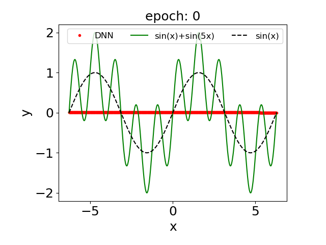
(a)

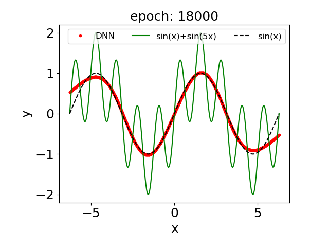
(b)

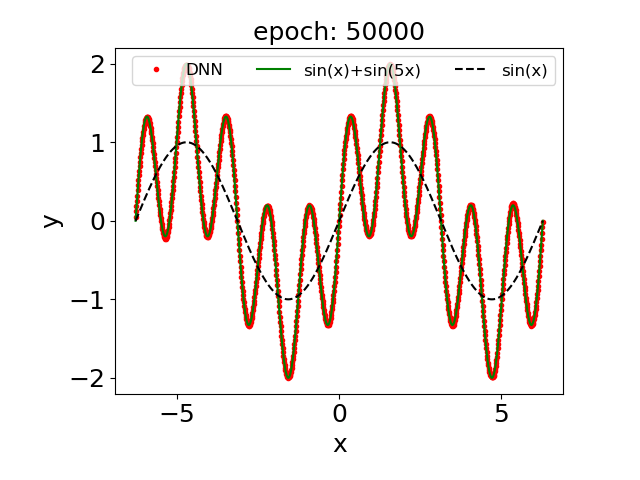
(c)

Figure 1: Illustration of the training process of a DNN. Training data are sampled from target function $\sin(x)+\sin(5x)$. Red, green and black curves indicates DNN output, $\sin(x)$, and $\sin(x)+\sin(5x)$ respectively.

1.2 Frequency principle

To visualize or characterize the training process in frequency domain, it requires a Fourier transform of the training data. However, the Fourier transform of high-dimensional data suffers from the curse of dimensionality and the visualization of high-dimensional data is difficult. Alternatively, one can study the problem of one-dimensional synthetic data. A series of experiments on synthetic low-dimensional data show that

• DNNs often fit target functions from low to high frequencies during the training.

This implicit frequency bias is named as frequency principle (F-Principle) (Xu et al., 2019, 2020; Zhang et al., 2021a) or spectral bias (Rahaman et al., 2019) and can be robustly observed no matter how overparameterized DNNs are. More experiments on real datasets are designed to confirm this observation (Xu et al., 2020). It is worthy to note that the frequency used here is a response frequency characterizing how the output is affected by the input. This frequency is easy to be confused in imaging classification problems. For example, in MNIST dataset, the frequency domain is also 784-dimensional but not 2-dimensional, i.e., the frequency of the classification function but not the image frequency w.r.t. 2-dimensional space.

Xu et al. (2020) proposed a key mechanism of the F-Principle that the regularity of the activation function converts into the decay rate of a loss function in the frequency domain. Theoretical studies subsequently show that the F-Principle holds in general setting with infinite samples (Luo et al., 2021a) and in the regime of wide DNNs (Neural Tangent Kernel (NTK) regime (Jacot et al., 2018)) with finite samples (Zhang et al., 2019, 2021a; Luo et al., 2020a) or samples distributed uniformly on sphere (Cao et al., 2021; Yang and Salman, 2019; Ronen et al., 2019; Bordelon et al., 2020). E et al. (2020) show that the integral equation would naturally leads to the F-Principle. In addition to characterizing the training speed of DNNs, the F-Principle also implicates that DNNs prefer low-frequency function and generalize well for low-frequency functions (Xu et al., 2020; Zhang et al., 2019, 2021a; Luo et al., 2020a).

The F-Principle further inspires the design of DNNs to fast learn a function with high frequency, such as in scientific computing and image or point cloud fitting problems (Liu et al., 2020; Jagtap et al., 2020; Cai et al., 2020; Tancik et al., 2020). In addition, the F-Principle provides a mechanism to understand many phenomena in applications and inspires a series of study on deep learning from frequency perspective. The study of deep learning is a highly inter-disciplinary problem. As an example, the Fourier analysis, an approach of signal processing, is an useful tool to understand better deep learning (Giryes and Bruna, 2020). A comprehensive understanding of deep learning remains an excited research subject calling for more fusion of existing approaches and developing new methods.

2 Empirical study of F-Principle

Before the discovery of the F-Principle, some works have suggested the learning of the DNNs may follow a order from simple to complex (Arpit et al., 2017). However, previous empirical studies focus on the real dataset, which is high-dimensional, thus, it is difficult to find a suitable quantity to characterize such intuition. In this section, we review the empirical study of the F-Principle, which first presents a clear picture from the one-dimensional data and then carefully designs experiments to verify the F-Principle in high-dimensional data (Xu et al., 2019, 2020; Rahaman et al., 2019).

2.1 One-dimensional experiments

To clearly illustrate the phenomenon of F-Principle, one can use $1$-d synthetic data to show the relative error of different frequencies during the training of DNN. The following shows an example from Xu et al. (2020).

Training samples are drawn from a $1$-d target function $f(x)=\sin(x)+\sin(3x)+\sin(5x)$ with three important frequency components and even space in $[-3.14,3.14]$, i.e., $\{x_{i},f(x_{i})\}_{i=0}^{n-1}$. The discrete Fourier transform (DFT) of $f(x)$ or the DNN output (denoted by $h(x)$) is computed by $\hat{f}_{k}=\frac{1}{n}\sum_{i=0}^{n-1}f(x_{i})\mathrm{e}^{-\mathrm{i}2\pi ik/n}$, where $k$ is the frequency. As shown in Fig. 2(a), the target function has three important frequencies as designed (black dots at the inset in Fig. 2(a)). To examine the convergence behavior of different frequency components during the training with MSE, one computes the relative difference between the DNN output and the target function for the three important frequencies at each recording step, that is, $\Delta_{F}(k)=|\hat{h}_{k}-\hat{f}_{k}|/|\hat{f}_{k}|$, where $|\cdot|$ denotes the norm of a complex number. As shown in Fig. 2(b), the DNN converges the first frequency peak very fast, while converging the second frequency peak much slower, followed by the third frequency peak.

A series of experiments are performed with relative cheap cost on synthetic data to verify the validity of the F-Principle and eliminate some misleading factors. For example, the stochasticity and the learning rate are not important to reproduce the F-Principle. If one only focuses on high-dimensional data, such as the simple MNIST, it would require a much more expensive cost of computation and computer memory to examine the impact of the stochasticity and the learning rate. The study of synthetic data shows a clear guidance to examine the F-Principle in the high-dimensional data. In addition, since frequency is a quantity which theoretical study is relative easy to access in, the F-Principle provides a theoretical direction for further study.

Figure 2: 1d input. (a) $f(x)$. Inset : $|\hat{f}(k)|$. (b) $\Delta_{F}(k)$ of three important frequencies (indicated by black dots in the inset of (a)) against different training epochs. Reprinted from Xu et al. (2020).

2.2 Two-dimensional experiments

An image can be regarded as a mapping from two-dimensional space coordinate to pixel intensity. The experiment in Fig. 3 uses a fully-connected DNN to fit the camera-man image in Fig. 3(a). The DNN learns from a coarse-grained image to one with more detail as the training proceeds, shown in Fig. 3(b-d). Obviously, this is also an order from low- to high-frequency, which is similar to how biological brain remembers an image. This 2d F-Principle example also shows that utilizing DNN to restore an image may take advantage of low-frequency preference, such as inpainting tasks, but also should be cautionary about its insufficiency in learning high-frequency structures. To overcome this insufficiency, some algorithms are developed (Chen et al., 2021a; Jiang et al., 2020; Xi et al., 2020; Tancik et al., 2020), which will be reviewed more in Section 6.2.

(a) True

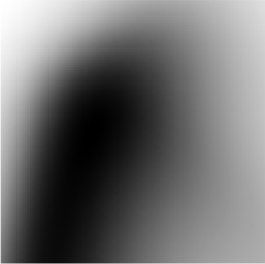
(b) step 80

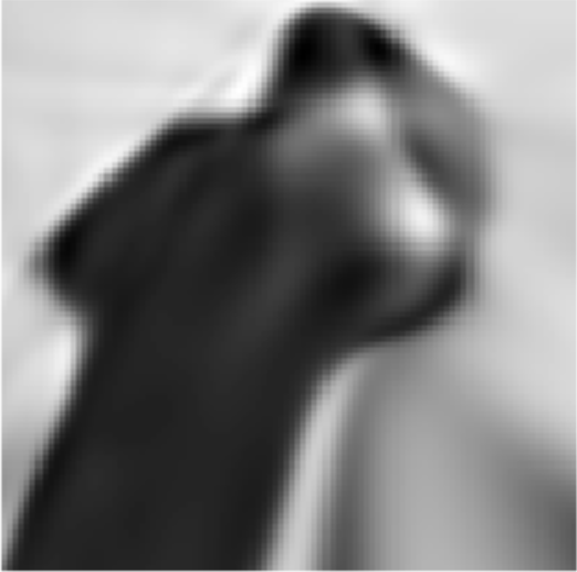
(c) step 2000

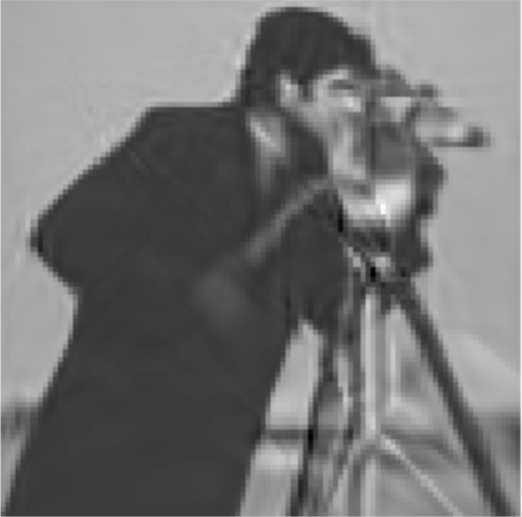
(d) step 58000

Figure 3: F-Principle in 2d datasets. Reprinted from Xu et al. (2020).

2.3 Frequency principle in high-dimensional problems

To study the F-Principle in high-dimensional data, two obstacles should be overcome first: what is the frequency in high dimension and how to separate different frequencies.

The concept of “frequency” often causes confusion in image classification problems. The image (or input) frequency (NOT used in the F-Principle of classification problems) is the frequency of $2$-d function $I:\mathbb{R}^{2}\to\mathbb{R}$ representing the intensity of an image over pixels at different locations. This frequency corresponds to the rate of change of intensity across neighbouring pixels. For example, an image of constant intensity possesses only the zero frequency, i.e., the lowest frequency, while a sharp edge contributes to high frequencies of the image.

The frequency used in the F-Principle of classification problems is also called response frequency of a general Input-Output mapping $f$. For example, consider a simplified classification problem of partial MNIST data using only the data with label $0$ and $1$, $f(x_{1},x_{2},\cdots,x_{784}):\mathbb{R}^{784}\to\{0,1\}$ mapping $784$-d space of pixel values to $1$-d space, where $x_{j}$ is the intensity of the $j$-th pixel. Denote the mapping’s Fourier transform as $\hat{f}(k_{1},k_{2},\cdots,k_{784})$. The frequency in the coordinate $k_{j}$ measures the rate of change of $f(x_{1},x_{2},\cdots,x_{784})$ with respect to $x_{j}$, i.e., the intensity of the $j$-th pixel. If $f$ possesses significant high frequencies for large $k_{j}$, then a small change of $x_{j}$ in the image might induce a large change of the output (e.g., adversarial example). For a real data, the response frequency is rigorously defined via the standard nonuniform discrete Fourier transform (NUDFT).

The difficulty of separating different frequencies is that the computation of Fourier transform of high-dimensional data suffers from the curse of dimensionality. For example, if one evaluates two points in each dimension of frequency space, then, the evaluation of the Fourier transform of a $d$-dimensional function is on $2^{d}$ points, an impossible large number even for MNIST data with $d=784$. Two approaches are proposed in (Xu et al., 2020).

2.3.1 Projection method

One approach is to study the frequency in one dimension of frequency space. For a dataset $\{(\bm{x}_{i},y_{i})\}_{i=0}^{n-1}$ with $y_{i}\in\mathbb{R}$. The high dimensional discrete non-uniform Fourier transform of $\{(\bm{x}_{i},y_{i})\}_{i=0}^{n-1}$ is $\hat{y}_{\bm{k}}=\frac{1}{n}\sum_{i=0}^{n-1}y_{i}\exp\left(-\mathrm{i}2\pi\bm{k}\cdot\bm{x}_{i}\right)$. Consider a direction of $\bm{k}$ in the Fourier space, i.e., $\bm{k}=k\bm{p}_{1}$, $\bm{p}_{1}$ is a chosen and fixed unit vector. Then we have $\hat{y}_{k}=\frac{1}{n}\sum_{i=0}^{n-1}y_{i}\exp\left(-\mathrm{i}2\pi(\bm{p}_{1}\cdot\bm{x}_{j})k\right)$, which is essentially the $1$-d Fourier transform of $\{(x_{\bm{p}_{1},i},y_{i})\}_{i=0}^{n-1}$, where $x_{\bm{p}_{1},i}=\bm{p}_{1}\cdot\bm{x}_{i}$ is the projection of $\bm{x}_{i}$ on the direction $\bm{p}_{1}$. Similarly, one can examine the relative difference between the DNN output and the target function for the selected important frequencies at each recording step. In the experiments in Xu et al. (2020), $\bm{p}_{1}$ is chosen as the first principle component of the input space. A fully-connected network and a convolutional network are used to learn MNIST and CIFAR10, respectively. As shown in Fig. 4(a) and 4(c), low frequencies dominate in both real datasets. As shown in Fig. 4(b) and 4(d), one can easily observe that DNNs capture low frequencies first and gradually capture higher frequencies.

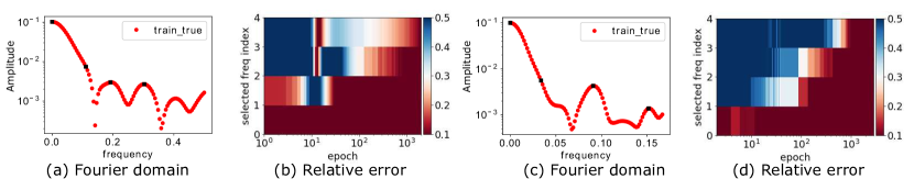
Figure 4: Projection method. (a, b) are for MNIST, (c, d) for CIFAR10. (a, c) Amplitude $|\hat{y}_{k}|$ vs. frequency. Selected frequencies are marked by black squares. (b, d) $\Delta_{F}(k)$ vs. training epochs for the selected frequencies. Reprinted from Xu et al. (2020).

2.3.2 Filtering method

The projection method examines the F-Principle at only several directions. To compensate the projection method, one can consider a coarse-grained filtering method which is able to unravel whether, in the radially averaged sense, low frequencies converge faster than high frequencies.

The idea of the filtering method is to use a Gaussian filter to derive the low-frequency part of the data and then examine the convergence of the low- and high-frequency parts separately. The low frequency part can be derived by

$$\bm{y}_{i}^{\mathrm{low},\delta}\triangleq(\bm{y}*G^{\delta})_{i},$$ (1)

where $*$ indicates convolution operator, $\delta$ is the standard deviation of the Gaussian kernel. Since the Fourier transform of a Gaussian function is still a Gaussian function but with a standard deviation $1/\delta$, $1/\delta$ can be regarded as a rough frequency width which is kept in the low-frequency part. The high-frequency part can be derived by

$$\bm{y}_{i}^{\mathrm{high},\delta}\triangleq\bm{y}_{i}-\bm{y}_{i}^{\mathrm{low},\delta}.$$ (2)

Then, one can examine

$$e_{\mathrm{low}}=\left(\frac{\sum_{i}|\bm{y}_{i}^{\mathrm{low},\delta}-\bm{h}_{i}^{\mathrm{low},\delta}|^{2}}{\sum_{i}|\bm{y}_{i}^{\mathrm{low},\delta}|^{2}}\right)^{\frac{1}{2}},$$ (3)

$$e_{\mathrm{high}}=\left(\frac{\sum_{i}|\bm{y}_{i}^{\mathrm{high},\delta}-\bm{h}_{i}^{\mathrm{high},\delta}|^{2}}{\sum_{i}|\bm{y}_{i}^{\mathrm{high},\delta}|^{2}}\right)^{\frac{1}{2}},$$ (4)

where $\bm{h}^{\mathrm{low},\delta}$ and $\bm{h}^{\mathrm{high},\delta}$ are obtained from the DNN output $\bm{h}$. If $e_{\mathrm{low}}<e_{\mathrm{high}}$ for different $\delta$’s during the training, F-Principle holds; otherwise, it is falsified. Note the DNN is trained as usual.

As shown in Fig. 5, low-frequency part converges faster in the following three settings for different $\delta$’s: a tanh fully-connected network for MNIST, a ReLU shallow convolutional network for CIFAR10, and a VGG16 (Simonyan and Zisserman, 2015) for CIFAR10.

Another approach to examine the F-Principle in high-dimensional data is to add noise to the training data and examine when the noise is captured by the network (Rahaman et al., 2019). Note that this approach contaminates the training data.

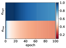
(a) $\delta=3$, DNN

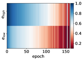
(b) $\delta=3$, CNN

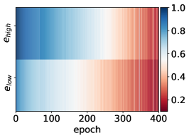
(c) $\delta=7$, VGG

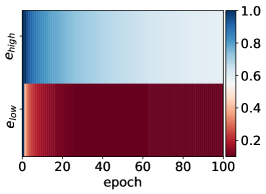
(d) $\delta=7$, DNN

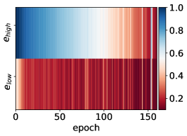
(e) $\delta=7$, CNN

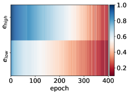
(f) $\delta=10$, VGG

Figure 5: F-Principle in real datasets. $e_{\mathrm{low}}$ and $e_{\mathrm{high}}$ indicated by color against training epoch. Reprinted from Xu et al. (2020).

3 Theoretical study of F-Principle

An advantage of studying DNNs from the frequency perspective is that frequency can often be theoretically analyzed. This is especially important in deep learning since deep learning is often criticized as a black box due to the the lack of theoretical support. In this section, we review theories of the F-Principle for various settings. A key mechanism of the F-Principle is based on the regularity of the activation function is first proposed in Xu (2018) and is formally published in Xu et al. (2020).

The theories has been developed to explore the F-Principle in an idealized setting (Xu et al., 2020), in general setting with infinite samples (Luo et al., 2021a), in a continuous viewpoint (E et al., 2020) and in the regime of wide DNNs (Neural Tangent Kernel (NTK) regime (Jacot et al., 2018)) with specific sample distributions (Cao et al., 2021; Yang and Salman, 2019; Ronen et al., 2019; Bordelon et al., 2020) or any finite samples (Zhang et al., 2019, 2021a; Luo et al., 2020a).

3.1 Intuitive analysis

3.1.1 Idealized setting for analyzing activation function

The following presents a simple case to illustrate how the F-Principles may arise. More details can be found in Xu (2018); Xu et al. (2020). The activation function we consider is $\sigma(x)=\tanh(x)$.

$$\sigma(x)=\tanh(x)=\frac{\mathrm{e}^{x}-\mathrm{e}^{-x}}{\mathrm{e}^{x}+\mathrm{e}^{-x}},\quad x\in\mathbb{R}.$$

For a DNN of one hidden layer with $m$ nodes, 1-d input $x$ and 1-d output:

$$h(x)=\sum_{j=1}^{m}a_{j}\sigma(w_{j}x+b_{j}),\quad a_{j},w_{j},b_{j}\in{\rm\mathbb{R}},$$ (5)

where $w_{j}$, $a_{j}$, and $b_{j}$ are training parameters. In the sequel, we will also use the notation $\theta=\{\theta_{lj}\}$ with $\theta_{1j}=a_{j}$, $\theta_{2j}=w_{j}$, and $\theta_{3j}=b_{j}$, $j=1,\cdots,m$. Note that the Fourier transform of $\tanh(x)$ is $\hat{\sigma}(k)=-\frac{\mathrm{i}\pi}{\sinh(\pi k/2)}$. The Fourier transform of $\sigma(w_{j}x+b_{j})$ with $w_{j},b_{j}\in{\rm\mathbb{R}}$, $j=1,\cdots,m$ reads as

$$\widehat{\sigma(w_{j}\cdot+b_{j})}(k)=\frac{2\pi\mathrm{i}}{|w_{j}|}\exp\Big{(}\frac{\mathrm{i}b_{j}k}{w_{j}}\Big{)}\frac{1}{\exp(-\frac{\pi k}{2w_{j}})-\exp(\frac{\pi k}{2w_{j}})}.$$ (6)

Note that the last term exponentially decays w.r.t. $|k|$. Thus

$$\hat{h}(k)=\sum_{j=1}^{m}\frac{2\pi a_{j}\mathrm{i}}{|w_{j}|}\exp\Big{(}\frac{\mathrm{i}b_{j}k}{w_{j}}\Big{)}\frac{1}{\exp(-\frac{\pi k}{2w_{j}})-\exp(\frac{\pi k}{2w_{j}})}.$$ (7)

Define the amplitude deviation between DNN output and the target function $f(x)$ at frequency $k$ as

$$D(k)\triangleq\hat{h}(k)-\hat{f}(k).$$

Write $D(k)$ as $D(k)=A(k)\mathrm{e}^{\mathrm{i}\phi(k)}$, where $A(k)\in[0,+\infty)$ and $\phi(k)\in\mathbb{R}$ are the amplitude and phase of $D(k)$, respectively. The loss at frequency $k$ is $L(k)=\frac{1}{2}\left|D(k)\right|^{2}$, where $|\cdot|$ denotes the norm of a complex number. The total loss function is defined as: $L=\int_{-\infty}^{+\infty}L(k)\mathop{}\!\mathrm{d}{k}$. Note that according to Parseval’s theorem, this loss function in the Fourier domain is equal to the commonly used loss of mean squared error, that is, $L=\int_{-\infty}^{+\infty}\frac{1}{2}(h(x)-f(x))^{2}\mathop{}\!\mathrm{d}{x}$.

The decrement along any direction, say, with respect to parameter $\theta_{lj}$, is

$$\frac{\partial L}{\partial\theta_{lj}}=\int_{-\infty}^{+\infty}\frac{\partial L(k)}{\partial\theta_{lj}}\mathop{}\!\mathrm{d}{k}.$$ (8)

The absolute contribution from frequency $k$ to this total amount at $\theta_{lj}$ is

$$\left|\frac{\partial L(k)}{\partial\theta_{lj}}\right|\approx A(k)\exp\left(-|\pi k/2w_{j}|\right)F_{lj}(\theta_{j},k),$$ (9)

where $\theta_{j}\triangleq\{w_{j},b_{j},a_{j}\}$, $\theta_{lj}\in\theta_{j}$, $F_{lj}(\theta_{j},k)$ is a function with respect to $\theta_{j}$ and $k$, which is approximate $O(1)$.

When the component at frequency $k$ where $\hat{h}(k)$ is not close enough to $\hat{f}(k)$, i.e., $A(k)\neq 0$, $\exp\left(-|\pi k/2w_{j}|\right)$ would dominate $G_{lj}(\theta_{j},k)$ for a small $w_{j}$. Intuitively, the gradient of low-frequency components dominates the training, thus, leading a fast convergence of low-frequency components.

The above analysis show the importance of the activation in the F-Principle. For most activations, such as tanh and RelU, they monotonically decay in the frequency domain. Therefore, we can easily observe F-Principle in Fig. 2. We can also design activation that does not monotonically decay in the frequency domain but monotonically increase up to a high frequency, where we expect to observe the frequency convergence order may flip up to a certain frequency. We use Ricker function with parameter $a$,

$$\frac{1}{15a}\pi^{1/4}\left(1-\left(\frac{x}{a}\right)^{2}\right)\exp\left(-\frac{1}{2}\left(\frac{x}{a}\right)^{2}\right).$$ (10)

With smaller $a$, Ricker function decays from a higher frequency. We perform similar learning task as Fig. 2. As shown in Fig. 6, in the first row, when the activation decays from a low frequency, we can clearly observe low frequency converges faster; however, in the second row, when the activation decays from a high frequency, we can not observe any frequency converges faster, which is consistent with our analysis.

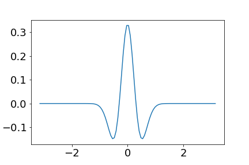
(a)

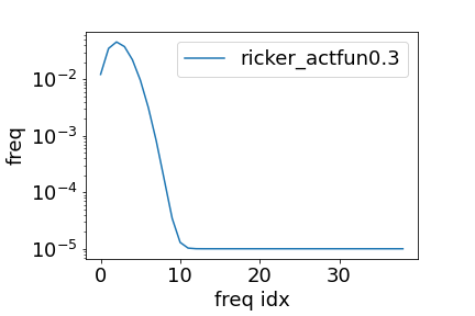
(b)

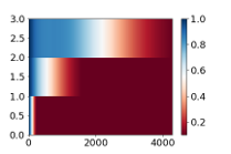
(c)

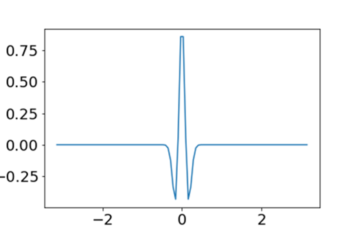
(d) activation in spatial domain

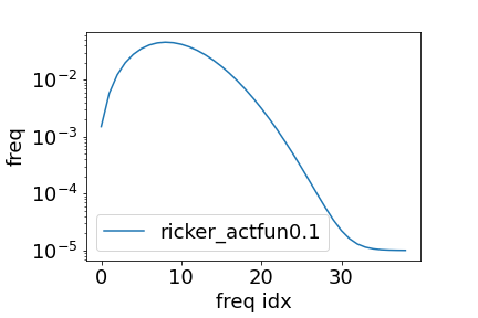
(e) activation in frequency domain

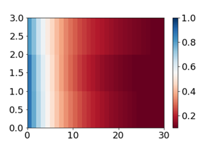
(f) convergence order

Figure 6: Ricker activation function. $a=0.3$ for the first row and $a=0.1$ for the second row.

3.1.2 Frequency weight in the loss function

The loss function form can affect the frequency convergence. For example, one can explicitly impose a large weight to some specific frequency component to accelerate the convergence of the frequency component. We consider two types of loss functions in learning the function as in Fig. 2, one is the common mean squared loss $L_{\rm nongrad}$, the other is one with an extra loss of gradient $L_{\rm nongrad}$,

$$L_{\rm nongrad}=\sum_{i=1}^{n}(f_{\theta}(x_{i})-f^{*}(x_{i}))^{2}/n,$$ (11)

$$L_{\rm nongrad}=L_{\rm nongrad}+\sum_{i=1}^{n}(\nabla_{x}f_{\theta}(x_{i})-\nabla_{x}f^{*}(x_{i}))^{2}/n.$$ (12)

As shown in Fig. 7, high frequency converges much faster in the case of the loss with gradient information. The key reason is that, the Fourier transform of $\nabla_{x}f_{\theta}(x_{i})$ is the product of the transform of $f_{\theta}(x_{i})$ and frequency $\xi$, which is equivalent to add more priority for higher frequency.

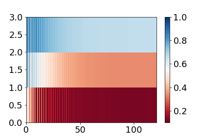
(a) $L_{\rm nongrad}$

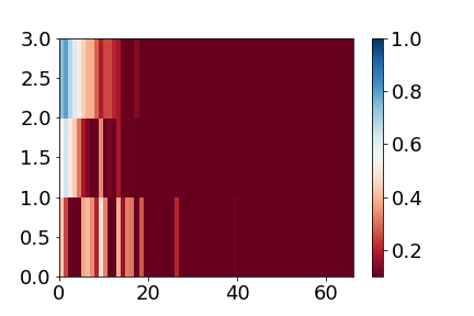
(b) $L_{\rm grad}$

Figure 7: The frequency convergence for networks with loss function $L_{\rm nongrad}$ and $L_{\rm grad}$.

3.1.3 The joint effect of activation and loss

The above analysis shows that the frequency convergence behavior is the joint effect of activation and loss. A more detailed analysis is shown in Eq. 62. For common loss functions and activation functions, F-Principle can be easily observed. However, in some specific setting or tasks, such as solving PDEs where the loss function often contains gradient information, F-Principle can be alleviated or disappear.

3.2 General setting

Luo et al. (2021a) consider DNNs trained by a general loss function $\tilde{R}_{\mathcal{D}}(\bm{\theta})$ and measure the convergence of different frequencies by a mean squared loss. Similarly to the filtering method, the basic idea in Luo et al. (2021a) is to decompose the frequency domain into a low-frequency part and a high-frequency part.

Based on the following assumptions, i.e., i) certain regularity of target function, sample distribution function and activation function; ii) bounded training trajectory with loss convergence. Luo et al. (2021a) prove that the change of high-frequency loss over the total loss decays with the separated frequency with a certain power, which is determined by the regularity assumption. A key ingredient in the proof is that the composition of functions still has a certain regularity, which renders the decay in frequency domain. This result thus holds for general network structure with multiple layers. Aside its generality, the characterization of the F-Principle is too coarse-grained to differentiate the effect network structure or the speciality of DNNs, but only gives a qualitative understanding.

E et al. (2020) present a continuous framework to study machine learning and suggests that the gradient flows of neural networks are nice flows, and they obey the frequency principle, basically because they are integral equations. The regularity of integral equations is higher, thus, leading to a faster decaying in the Fourier domain.

3.3 NTK setting and linear F-Principle

In general, it is difficult to analyze the convergence rate of each frequency due to its high dimensionality and nonlinearity. However, in a linear NTK regime (Jacot et al., 2018), where the network has a width $m$ approaching infinite and a scaling factor of $1/\sqrt{m}$, several works have explicitly shown the convergence rate of each frequency.

3.3.1 NTK dynamics

One can consider the following gradient-descent flow dynamics of the empirical risk $L_{S}$ of a network function $f(\cdot,\bm{\theta})$ parameterized by $\bm{\theta}$ on a set of training data $\{(\bm{x}_{i},y_{i})\}_{i=1}^{n}$

$$\left\{\begin{array}[]{l}\dot{\bm{\theta}}=-\nabla_{\bm{\theta}}L_{S}(\bm{\theta}),\\ \bm{\theta}(0)=\bm{\theta}_{0},\end{array}\right.$$ (13)

where

$$L_{S}(\bm{\theta})=\frac{1}{2}\sum_{i=1}^{n}(f(\bm{x}_{i},\bm{\theta})-y_{i})^{2}.$$ (14)

Then the training dynamics of output function $f(\cdot,\bm{\theta})$ is

$$\frac{\mathrm{d}}{\mathrm{d}t}f(\bm{x},\bm{\theta}) =\nabla_{\bm{\theta}}f(\bm{x},\bm{\theta})\cdot\dot{\bm{\theta}}$$

$$=-\nabla_{\bm{\theta}}f(\bm{x},\bm{\theta})\cdot\nabla_{\bm{\theta}}L_{S}(\bm{\theta})$$

$$=-\nabla_{\bm{\theta}}f(\bm{x},\bm{\theta})\cdot\sum_{i=1}^{n}\nabla_{\bm{\theta}}f(\bm{x}_{i},\bm{\theta})(f(\bm{x}_{i},\bm{\theta})-y_{i})$$

$$=-\sum_{i=1}^{n}K_{m}(\bm{x},\bm{x}_{i})(f(\bm{x}_{i},\bm{\theta})-y_{i})$$

where for time $t$ the NTK evaluated at $(\bm{x},\bm{x}^{\prime})\in\Omega\times\Omega$ reads as

$$K_{m}(\bm{x},\bm{x}^{\prime})(t)=\nabla_{\bm{\theta}}f(\bm{x},\bm{\theta}(t))\cdot\nabla_{\bm{\theta}}f(\bm{x}^{\prime},\bm{\theta}(t)).$$ (15)

As the NTK regime studies the network with infinite width, we denote

$$K^{*}(\bm{x},\bm{x}^{\prime})(t):=\lim_{m\rightarrow\infty}K_{m}(\bm{x},\bm{x}^{\prime})(t)$$ (16)

The gradient descent of the model thus becomes

$$\frac{\mathrm{d}}{\mathrm{d}t}\Big{(}f(\bm{x},\bm{\theta}(t))-f(\bm{x})\Big{)}=-\sum_{i=1}^{n}K^{*}(\bm{x},\bm{x}_{i})(t)\Big{(}f(\bm{x}_{i},\bm{\theta}(t))-f(\bm{x}_{i})\Big{)}.$$ (17)

Define the residual $\bm{u}(\bm{x},t)=f(\bm{x},\bm{\theta}(t))-f(\bm{x})$. Denote $\bm{X}\in\mathbb{R}^{n\times d}$ and $\bm{Y}\in\mathbb{R}^{n}$ as the training data, $u(\bm{X}),\nabla_{\bm{\theta}}f(\bm{X},\bm{\theta}(t))\in\mathbb{R}^{n}$, and

$$K^{*}(t)=\lim_{m\rightarrow\infty}K_{m}(t):=\lim_{m\rightarrow\infty}\nabla_{\bm{\theta}}f(\bm{X},\bm{\theta}(t))(\nabla_{\bm{\theta}}f(\bm{X},\bm{\theta}(t)))^{T}\in\mathbb{R}^{n\times n}.$$ (18)

Then, one can obtain

$$\frac{\mathrm{d}u(\bm{X})}{\mathrm{d}t}=-K^{*}(t)u(\bm{X}).$$ (19)

In a continuous form, one can define the empirical density $\rho(\bm{x})=\sum_{i=1}^{n}\delta(\bm{x}-\bm{x}_{i})/n$ and further denote $u_{\rho}(\bm{x})=u(\bm{x})\rho(\bm{x})$. Therefore the dynamics for $u$ becomes

$$\frac{\mathrm{d}}{\mathrm{d}t}u(\bm{x},t)=-\int_{\mathbb{R}^{d}}K^{*}(\bm{x},\bm{x}^{\prime})(t)u_{\rho}(\bm{x}^{\prime},t)\mathop{}\!\mathrm{d}{\bm{x}^{\prime}}.$$ (20)

Note that here we slightly abuse the usage of notation $K^{*}$. This continuous form renders an integral equation analyzed in E et al. (2020).

The convergence analysis of the dynamics in Eq. (19) can be done by performing eigen decomposition of $K^{*}$. The component in the sub-space of an eigen-vector converges faster with a larger eigen-value. For two-layer wide DNNs in NTK regime, one can derive $K^{*}(t)\sim K^{*}(0)$. A series of works further show that the eigenvector with a larger eigen-value is lower-frequency, therefore, providing a rigorous proof for the F-Principle in NTK regime for two-layer networks.

Consider a two-layer DNN

$$f(\bm{x},\bm{\theta}) =\frac{1}{\sqrt{m}}\sum_{j=1}^{m}a_{j}\sigma(\bm{w}_{j}^{\intercal}\bm{x}+b_{j}),$$ (21)

where the vector of all parameters $\bm{\theta}$ is formed of the parameters for each neuron ${(a_{j},\bm{w}_{j}^{\intercal},b_{j})}^{\intercal}\in\mathbb{R}^{d+2}$ for $j\in[m]$. At the infinite neuron limit $m\to\infty$, the following linearization around initialization

$$f^{{\rm lin}}\left(\bm{x};\bm{\theta}(t)\right)=f\left(\bm{x};\bm{\theta}(0)\right)+\nabla_{\bm{\theta}}f\left(\bm{x};\bm{\theta}(0)\right)\left(\bm{\theta}(t)-\bm{\theta}(0)\right)$$ (22)

is an effective approximation of $f\left(\bm{x};\bm{\theta}(t)\right)$, i.e., $f^{{\rm lin}}\left(\bm{x};\bm{\theta}(t)\right)\approx f\left(\bm{x};\bm{\theta}(t)\right)$ for any $t$, as demonstrated by both theoretical and empirical studies of neural tangent kernels (NTK) (Jacot et al., 2018; Lee et al., 2019). Note that, $f^{{\rm lin}}\left(\bm{x};\bm{\theta}(t)\right)$, linear in $\bm{\theta}$ and nonlinear in $\bm{x}$, reserves the universal approximation power of $f\left(\bm{x};\bm{\theta}(t)\right)$ at $m\to\infty$. In the following of this sub-section, we do not distinguish $f\left(\bm{x};\bm{\theta}(t)\right)$ from $f^{{\rm lin}}\left(\bm{x};\bm{\theta}(t)\right)$.

3.3.2 Eigen analysis for two-layer DNN with dense data distribution

For two-layer ReLU network, $K^{*}$ enjoys good properties for theoretical study. The exact form of $K^{*}$ can be theoretically obtained (Xie et al., 2017). Under the condition that training samples distributed uniformly on a sphere, the spectrum of $K^{*}$ can be obtained through spherical harmonic decomposition (Xie et al., 2017). In a rough intuition, each eigen-vector of $K^{*}$ corresponds to a specific frequency. Based on such harmonic analysis, Ronen et al. (2019); Cao et al. (2021) estimate the eigen values of $K^{*}$, i.e., the convergence rate of each frequency. Basri et al. (2020) further release the condition that data distributed uniformly on a sphere to that data distributed piecewise constant on a sphere but limit the result on 1d sphere. Similarly under the uniform distribution assumption in NTK regime, Bordelon et al. (2020) show that as the size of the training set grows, ReLU DNNs fit successively higher spectral modes of the target function. Empirical studies also validate that real data often align with the eigen-vectors that have large eigen-values, i.e., low frequency eigen-vectors (Dong et al., 2019; Kopitkov and Indelman, 2020; Baratin et al., 2020).

3.3.3 Linear F-Principle for two-layer neural network with arbitrary data distribution

The condition of dense distribution, such as uniform on a sphere, is often non-realistic in a training. A parallel work (Zhang et al., 2019, 2021a) studies the evolution of each frequency for two-layer wide ReLU networks with any data distribution, including randomly discrete case, and derive the linear F-Principle (LFP) model. Luo et al. (2020b) provides a rigorous version of Zhang et al. (2019, 2021a) and extend the study of ReLU activation function in Zhang et al. (2019, 2021a) to general activation functions.

The key idea is to perform Fourier transform of the kernel $K^{*}(\bm{x},\bm{x}^{\prime})$ w.r.t. both $\bm{x}$ and $\bm{x}^{\prime}$. To separate the evolution of each frequency, one has to assume the bias is significantly larger than $1$. In numerical experiments, by taking the order of bias as the maximum of the input weight and the output weight, one can obtains an accurate approximation of two-layer DNNs with LFP.

We use a LFP result for two-layer ReLU network for intuitive understanding. Consider the residual $\bm{u}(\bm{x},t)=f(\bm{x},\bm{\theta}(t))-f^{*}(\bm{x})$, one can obtain

$$\partial_{t}\hat{u}=-(\gamma(\bm{\xi}))^{2}\hat{u_{\rho}}(\bm{\xi}),$$ (23)

with

$$(\gamma(\bm{\xi}))^{2}=\frac{C_{1}}{\lVert\bm{\xi}\rVert^{d+3}}+\frac{C_{2}}{\lVert\bm{\xi}\rVert^{d+1}},$$ (24)

where $\hat{\cdot}$ is Fourier transform, $C_{1}$ and $C_{2}$ are constants depending on the initial distribution of parameters, $(\cdot)_{\rho}(\bm{x}):=(\cdot)(\bm{x})\rho(\bm{x})$. $\rho(\bm{x})$ is the data distribution, which can be a continuous function or $\rho(\bm{x})=\Sigma_{i=1}^{n}\delta(\bm{x}-\bm{x}_{i})/n$.

One can further prove that the long-time solution of (23) satisfies the following constrained minimization problem

$$\min_{h} \int\gamma(\bm{\xi})^{-2}|\hat{h}(\bm{\xi})-\hat{h}_{\rm ini}(\bm{\xi})|^{2}\mathop{}\!\mathrm{d}{\bm{\xi}},$$ (25)

$${\rm s.t.} h(\bm{x}_{i})=f^{*}(\bm{x}_{i}),\;i=1,\ldots,n.$$

Based on the equivalent optimization problem in (25), each decaying term for 1-d problems ($d=1$) can be analyzed. When $1/\xi^{2}$ term dominates, the corresponding minimization problem Eq. (25) rewritten into spatial domain yields

$$\min_{h}\int|h^{{}^{\prime}}(x)-h_{\rm ini}^{{}^{\prime}}(x)|^{2}\mathop{}\!\mathrm{d}{x},$$ (26)

$${\rm s.t.} \quad h(\bm{x}_{i})=f^{*}(\bm{x}_{i}),i=1,\cdots,n,$$

where ^′ indicates differentiation. For $h_{\rm ini}(x)=0$, Eq. (26) indicates a linear spline interpolation. Similarly, when $1/\xi^{4}$ dominates, $\int|h^{{}^{\prime\prime}}(x)-h_{\rm ini}^{{}^{\prime\prime}}(x)|^{2}\mathop{}\!\mathrm{d}{x}$ is minimized, indicating a cubic spline. In general, above two power law decay coexist, giving rise to a specific mixture of linear and cubic splines. For high dimensional problems, the model prediction is difficult to interpret because the order of differentiation depends on $d$ and can be fractal. Similar analysis in spatial domain can be found in a subsequent work in Jin and Montúfar (2020).

Inspired by the variational formulation of LFP model in (25), Luo et al. (2020c) propose a new continuum model for the supervised learning. This is a variational problem with a parameter $\alpha>0$:

$$\min_{h\in\mathcal{H}}Q_{\alpha}[h]=\int_{\mathbb{R}^{d}}\langle\bm{\xi}\rangle^{\alpha}\left\lvert\hat{h}(\bm{\xi})\right\rvert^{2}\mathop{}\!\mathrm{d}{\bm{\xi}},$$ (27)

$$\mathrm{s.t.}\quad h(\bm{x}_{i})=y_{i},\quad i=1,\cdots,n,$$ (28)

where $\langle\bm{\xi}\rangle=(1+\lVert\bm{\xi}\rVert^{2})^{\frac{1}{2}}$ is the “Japanese bracket” of $\bm{\xi}$ and $\mathcal{H}=\{h(x)|\int_{\mathbb{R}^{d}}\langle\bm{\xi}\rangle^{\alpha}\left\lvert\hat{h}(\bm{\xi})\right\rvert^{2}\mathop{}\!\mathrm{d}{\bm{\xi}}<\infty\}$.

Luo et al. (2020c) prove that $\alpha=d$ is a critical point. If $\alpha<d$, the variational problem leads to a trivial solution that is only non-zero at the training data point. If $\alpha>d$, the variational problem leads to a solution with certain regularity. The LFP model shows that a DNN is a convenient way to implement the variational formulation, which automatically satisfies the well-posedness condition.

Finally, we give some remarks on the difference between the eigen decomposition and the frequency decomposition. In the non-NTK regime, the eigen decomposition can be similarly analyzed but without informative explicit form. In addition, the study of bias from the perspective of eigen decomposition is very limited. For finite networks, which are practically used, the kernel evolves with training, thus, it is hard to understand what kind of the component converges faster or slower. The eigen mode of the kernel is also difficult to be perceived. In the contrast, frequency decomposition is easy to be interpreted, and a natural approach widely used in science.

4 Generalization

Generalization is a central issue of deep learning. In this section, we review how F-Principle gains understandings to the non-overfitting puzzle of over-parameterized DNN in deep learning (Zhang et al., 2017). First, we show that DNNs without F-Principle would end up with oscillated output in synthetic example. Second, we show how intuitively the F-Principle explains a strength and a weakness of deep learning (Xu et al., 2020). Third, we provide a rationale for the common trick of early-stopping (Xu et al., 2019), which is often used to improve the generalization. Fourth, we estimate an a priori generalization error bound for wide two-layer ReLU DNN (Luo et al., 2020b). Fifth, we discuss the effect of the F-Principle in alleviating the overfitting in Runge’s phenomenon.

4.1 DNN without F-Principle produces oscillated output

To examine the utility of the F-Principle, we compare DNNs outputs for two experiments in Fig. 6. For the one with F-Principle, as shown in Fig. 8, the initial output is smooth in (a), the DNN learns the training data well in (b), and the DNN output is smooth at test points in (c). However, for the one without the F-Principle, the initial output is rather oscillated in (d), the DNN can also learns the training data well in (e), but it is very oscillated with larger amplitude than the initial output at test points in (f). Apparently, such oscillated output usually leads to bad generalization. This example shows the F-Principle is an necessary condition underlying the good generalization of DNNs.

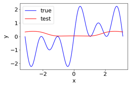
(a) initial output

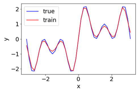
(b) final train output

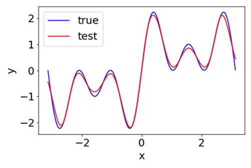
(c) final test output

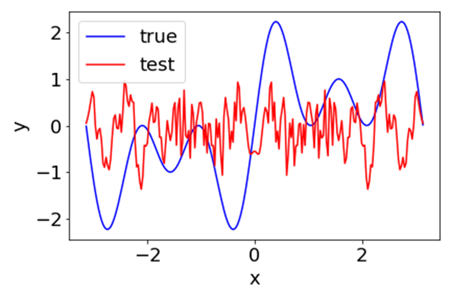
(d) initial output

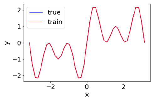
(e) final train output

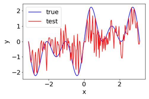
(f) final test output

Figure 8: DNN outputs with Ricker activation function. $a=0.3$ for the first row and $a=0.1$ for the second row. Same experiments as Fig. 6.

4.2 Strength and weakness

As demonstrated in the Introduction part, if the implicit bias or characteristics of an algorithm is consistent with the property of data, the algorithm generalizes well, otherwise not. By identifying the implicit bias of the DNNs in F-Principle, we can have a better understanding to the strength and the weakness of deep learning, as demonstrated by Xu et al. (2020) in the following.

DNNs often generalize well for real problems Zhang et al. (2017) but poorly for problems like fitting a parity function Shalev-Shwartz et al. (2017); Nye and Saxe (2018) despite excellent training accuracy for all problems. The following demonstrates a qualitative difference between these two types of problems through Fourier analysis and use the F-Principle to provide an explanation different generalization performances of DNNs.

Using the projection method in Sec. 2.3.1, one can obtain frequencies along the examined directions. For illustration, the Fourier transform of all MNIST/CIFAR10 data along the first principle component are shown in Fig. 9(a, b) for MNIST/CIFAR10, respectively. The Fourier transform of the training data (red dot) well overlaps with that of the total data (green) at the dominant low frequencies. As expected, the Fourier transform of the DNN output with bias of low frequency, evaluated on both training and test data, also overlaps with the true Fourier transform at low-frequency part. Due to the negligible high frequency in these problems, the DNNs generalize well.

However, DNNs generalize badly for high-frequency functions as follows. For the parity function $f(\bm{x})=\prod_{j=1}^{d}x_{j}$ defined on $\Omega=\{-1,1\}^{d}$, its Fourier transform is $\hat{f}(\bm{k})=\frac{1}{2^{d}}\sum_{x\in\Omega}\prod_{j=1}^{d}x_{j}\mathrm{e}^{-\mathrm{i}2\pi\bm{k}\cdot\bm{x}}=(-\mathrm{i})^{d}\prod_{j=1}^{d}\sin 2\pi k_{j}$. Clearly, for $\bm{k}\in[-\frac{1}{4},\frac{1}{4}]^{d}$, the power of the parity function concentrates at $\bm{k}\in\{-\frac{1}{4},\frac{1}{4}\}^{d}$ and vanishes as $\bm{k}\to\bm{0}$, as illustrated in Fig. 9(c) for the direction of $\bm{1}_{d}$. Given a randomly sampled training dataset $S\subset\Omega$ with $s$ points, the nonuniform Fourier transform on $S$ is computed as $\hat{f}_{S}(\bm{k})=\frac{1}{s}\sum_{x\in S}\prod_{j=1}^{d}x_{j}\mathrm{e}^{-\mathrm{i}2\pi\bm{k}\cdot\bm{x}}$. As shown in Fig. 9(c), $\hat{f}(\bm{k})$ and $\hat{f}_{S}(\bm{k})$ significantly differ at low frequencies, caused by the well-known aliasing effect. Based on the F-Principle, as demonstrated in Fig. 9(c), these artificial low frequency components will be first captured to explain the training samples, whereas the high frequency components will be compromised by DNN, leading to a bad generalization performance as observed in experiments.

The F-Principle implicates that among all the functions that can fit the training data, a DNN is implicitly biased during the training towards a function with more power at low frequencies, which is consistent as the implication of the equivalent optimization problem (25). The distribution of power in Fourier domain of above two types of problems exhibits significant differences, which result in different generalization performances of DNNs according to the F-Principle.

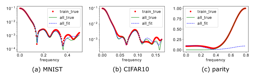
Figure 9: Fourier analysis for different generalization ability. The plot is the amplitude of the Fourier coefficient against frequency $k$. The red dots are for the training dataset, the green line is for the whole dataset, and the blue dashed line is for an output of well-trained DNN on the input of the whole dataset. For (c), $d=10$. The training data is $200$ randomly selected points. The settings of (a) and (b) are the same as the ones in Fig. 4. For (c), we use a tanh-DNN with widths 10-500-100-1, learning rate $0.0005$ under full batch-size training by Adam optimizer. The parameters of the DNN are initialized by a Gaussian distribution with mean $0$ and standard deviation $0.05$. Reprinted from Xu et al. (2020).

4.3 Early stopping

When the training data is contaminated by noise, early-stopping method is usually applied to avoid overfitting in practice (Lin et al., 2016). By the F-Principle, early-stopping can help avoid fitting the noisy high-frequency components. Thus, it naturally leads to a well-generalized solution. Xu et al. (2019) use the following example for illustration.

As shown in Fig. 10(a), the data are sampled from a function with noise. The DNN can well fit the sampled training set as the loss function of the training set decreases to a very small value (green stars in Fig. 10(b)). However, the loss function of the test set first decreases and then increases (red dots in Fig. 10(b)). Fig. 10(c), the Fourier transform for the training data (red) and the test data (black) only overlap around the dominant low-frequency components. Clearly, the high-frequency components of the training set are severely contaminated by noise. Around the turning step — where the best generalization performance is achieved, indicated by the green dashed line in Fig. 10(b) — the DNN output is a smooth function (blue line in Fig. 10(a)) in spatial domain and well captures the dominant peak in frequency domain (Fig. 10 (c)). After that, the loss function of the test set increases as DNN start to capture the higher-frequency noise (red dots in Fig. 10b). These phenomena conform with our analysis that early-stopping can lead to a better generalization performance of DNNs as it helps prevent fitting the noisy high-frequency components of the training set.

As a low-frequency function is more robust w.r.t. input than a high-frequency frequency function, the early-stopping can also enhance the robustness of the DNN. This effect is consistent with the study in Li et al. (2020a), which show that a two-layer DNN, trained only on the input weight and early stopped, can reconstruct the true labels from a noisy data.

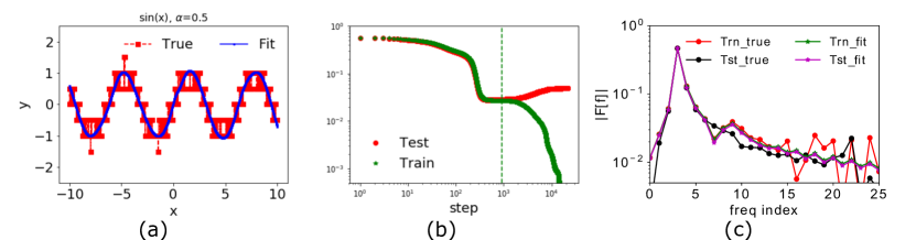
Figure 10: Effect of early-stopping on contaminated data. The training set and the test set consist of $300$ and $6000$ data points evenly sampled in $[-10,10]$, respectively. (a) The sampled values of the test set (red square dashed line) and DNN outputs (blue solid line) at the turning step. (b) Loss functions for training set (green stars) and test set (red dots) at different recording steps. The green dashed line is drawn at the turning step, where the best generalization performance is achieved. (c) The Fourier transform of the true data for the training set (red) and test set (black), and the Fourier transform of the DNN output for the training set (green), and test set (magenta) at the turning step. Reprinted from Xu et al. (2019).

4.4 Quantitative understanding in NTK regime

The static minimization problem (25) defines an FP-energy $E_{\gamma}(h)=\int\gamma^{-2}|\hat{h}|^{2}\mathop{}\!\mathrm{d}{\bm{\xi}}$ that quantifies the preference of the LFP model among all its steady states. Because $\gamma(\bm{\xi})^{-2}$ is an increasing function, say $\gamma(\bm{\xi})^{-2}=\lVert\bm{\xi}\rVert^{d+1}$, the FP-energy $\int\lVert\bm{\xi}\rVert^{d+1}|\hat{h}|^{2}\mathop{}\!\mathrm{d}{\bm{\xi}}$ amplifies the high frequencies while diminishing low frequencies. By minimizing $E_{\gamma}(h)$, problem (25) gives rise to a low frequency fitting, instead of an arbitrary one, of training data. By intuition, if target $f^{*}$ is indeed low frequency dominant, then $h_{\infty}$ likely well approximates $f^{*}$ at unobserved positions.

To theoretically demonstrate above intuition, Luo et al. (2020b) derive in the following an estimate of the generalization error of $h_{\infty}$ using the a priori error estimate technique (E et al., 2019). Because $h(\bm{x})=f^{*}(\bm{x})$ is a viable steady state, $E_{\gamma}(h_{\infty})\leq E_{\gamma}(f^{*})$ by the minimization problem. Using this constraint on $h_{\infty}$, one can obtain that, with probability of at least $1-\delta$,

$$\mathbb{E}_{\bm{x}}(h_{\infty}(\bm{x})-f^{*}(\bm{x}))^{2}\leq\frac{E_{\gamma}(f^{*})}{\sqrt{n}}C_{\gamma}\left(2+4\sqrt{2\log(4/\delta)}\right),$$ (29)

where $C_{\gamma}$ is a constant depending on $\gamma$. Error reduces with more training data as expected with a decay rate $1/\sqrt{n}$ similar to Monte-Carlo method. Importantly, because $E_{\gamma}(f^{*})$ strongly amplifies high frequencies of $f^{*}$, the more high-frequency components the target function $f^{*}$ possesses, the worse $h_{\infty}$ may generalize.

Note that the error estimate is also consistent with another result (Arora et al., 2019) published at similar time. Arora et al. (2019) prove that the generalization error of the two-layer ReLU network in NTK regime found by GD is at most

$$\sqrt{\frac{2Y^{T}(K^{*})^{-1}Y}{n}},$$ (30)

where $K^{*}$ is defined in (18), $Y\in\mathbb{R}^{n}$ is the labels of $n$ training data. If the data $Y$ is dominated more by the component of the eigen-vector that has small eigen-value, then, the above quantity is larger. Since in NTK regime the eigen-vector that has small eigen-value corresponds to a higher frequency, the error bound in (29) is larger, consistent with (30).

4.5 Runge’s phenomenon

In numerical analysis, Runge’s phenomenon is that oscillation at the edges of an interval would occur when using polynomial interpolation with polynomials of high degree over a set of equispaced interpolation points. Consider using mean squared loss and gradient descent to find the solution of a such polynomial interpolation. Since the solution is unique, the GD with infinite training time would find a some solution that produces Runge’s phenomenon. However, similar to the analysis of the F-Principle in the ideal case, apparently, the F-Principle should hold, as shown in Fig. 11. This example shows that the F-Principle can co-exist with Runge’s phenomenon, a clear over-fitting case. However, as the example of early-stopping shows, the F-Principle can help alleviate the overfitting by early-stopping. Similar analysis for why the double descent is rarely seen in DNN is analyzed in Ma et al. (2020).

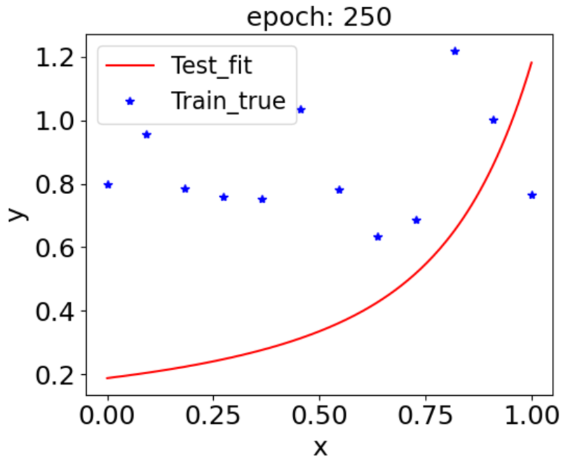
(a)

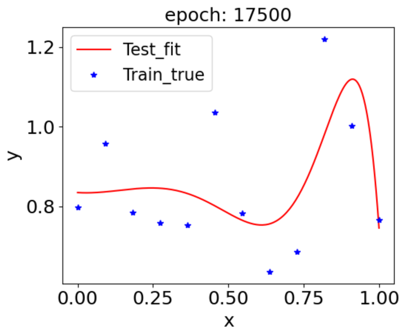
(b)

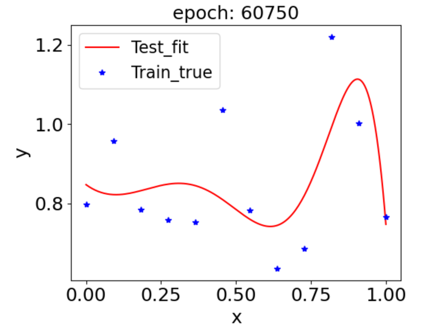
(c)

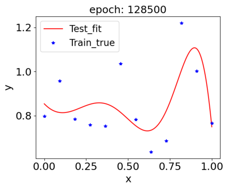
(d)

Figure 11: Using mean squared loss and gradient descent to find the solution of a polynomial interpolation with order 11 and 12 equispaced points.

5 F-Principle for scientific computing

Recently, DNN-based approaches have been actively explored for a variety of scientific computing problems, e.g., solving high-dimensional partial differential equations (E et al., 2017; Khoo and Ying, 2019; He et al., 2018; Fan et al., 2019; Han et al., 2019; Weinan et al., 2018; He and Xu, 2019; Strofer et al., 2019) and molecular dynamics (MD) simulations (Han et al., 2018). For solving PDEs, one can use DNNs to parameterize the solution of a specific PDE (Dissanayake and Phan-Thien, 1994; E et al., 2017; Raissi et al., 2019; Zang et al., 2020) or the operator of a type of PDE (Fan et al., 2019; Li et al., 2020b; Lu et al., 2021a; Zhang et al., 2021b). An overview of using DNN to solve high-dimensional PDEs can be found in E et al. (2021). We would focus on former approach.

F-Principle is an important characteristic of DNN-based algorithms. In this section, we will first review the frequency convergence difference between DNN-based algorithm and conventional methods, i.e., iterative methods and finite element method. Then, we rationalize their difference and understand the F-Principle from the iterative perspective. Finally, we review algorithms developed for overcoming the curse of high-frequency in DNN-based methods.

5.1 Parameterize the solution of a PDE

For intuitive illustration, we use Poisson’s equation as an example, which has broad applications in mechanical engineering and theoretical physics Evans (2010),

$$-\Delta u(\bm{x})=g(\bm{x}),\quad\bm{x}\in\Omega,$$ (31)

with the boundary condition

$$u(\bm{x})=\tilde{g}(\bm{x}),\quad\bm{x}\in\partial\Omega.$$ (32)

One can use a neural network $u(\bm{x};\bm{\theta})$, where $\bm{\theta}$ is the set of DNN parameters. A deep Ritz approach E and Yu (2018) utilize the following variational problem

$$u^{*}=\arg\min_{v}J(v),$$ (33)

where the solution of the above minimization problem can be prove to be the solution of the Possion’s problem and the energy functional is defined as

$$J(v)=\int_{\Omega}\left(\frac{1}{2}|\nabla v|^{2}+V(\bm{r})v^{2}\right)d\bm{r}-{\displaystyle\int\limits_{\Omega}}g(\mathbf{r})v(\mathbf{r})d\bm{r}\triangleq{\displaystyle\int\limits_{\Omega}}E(v(\mathbf{r}))dr.$$ (34)

In simulation, the Ritz loss function for training a DNN $u(\bm{x};\bm{\theta})$, which parameterizes the solution of the Possion’s problem, is chosen to be

$$L_{\rm ritz}(\bm{\theta})=\frac{1}{n}\sum_{\bm{x}\in S}(|\nabla u(\bm{x};\bm{\theta})|^{2}/2-g(\bm{x})u(\bm{x};\bm{\theta}))+\frac{\beta}{\tilde{n}}\sum_{\bm{x}\in\tilde{S}}(u(\bm{x};\bm{\theta})-\tilde{g}(\bm{x}))^{2},$$ (35)

where $S$ is the sample set from $\Omega$ and $n$ is the sample size, $\tilde{n}$ indicates sample set from $\partial\Omega$. The second penalty term with a weight $\beta$ is to enforce the boundary condition.

A more direct method, also known as physics-informed neural network (PINN) or least squared method, use the following loss function. In an alternative approach, one can simply use the loss function of Least Squared Error (LSE) ,

$$L_{\rm LSE}(\bm{\theta})=\frac{1}{n}\sum_{\bm{x}\in S}(\Delta u(\bm{x};\bm{\theta})+g(\bm{x}))^{2}+\frac{\beta}{\tilde{n}}\sum_{\bm{x}\in\tilde{S}}(u(\bm{x};\bm{\theta})-\tilde{g}(\bm{x}))^{2}.$$ (36)

To see the learning accuracy, one can compute the distance between $u(\bm{x};\bm{\theta})$ and $u_{\rm true}$,

$${\rm MSE}(u(\bm{x};\bm{\theta}),u_{\rm true}(\bm{x}))=\frac{1}{n+\tilde{n}}\sum_{\bm{x}\in S\cup\tilde{S}}(u(\bm{x};\bm{\theta})-u_{\rm true}(\bm{x}))^{2}.$$ (37)

5.2 Difference from conventional algorithms

5.2.1 Iterative methods

A stark difference between a DNN-based solver and the Jacobi method during the training/iteration is that DNNs learns the solution from low- to high-frequency (Xu et al., 2020), while Jacobi method learns the solution from high- to low-frequency. Therefore, DNNs would suffer from high-frequency curse.

Jacobi method

Before we show the difference between a DNN-based solver and the Jacobi method, we illustrate the procedure of the Jacobi method.

Consider a $1$-d Poisson’s equation:

$$-\Delta u(x)=g(x),\quad x\in\Omega\triangleq(-1,1),$$ (38)

$$u(-1)=u(1)=0.$$ (39)

$[-1,1]$ is uniformly discretized into $n+1$ points with grid size $h=2/n$. The Poisson’s equation in Eq. (38) can be solved by the central difference scheme,

$$-\Delta u_{i}=-\frac{u_{i+1}-2u_{i}+u_{i-1}}{h^{2}}=g(x_{i}),\quad i=1,2,\cdots,n,$$ (40)

resulting a linear system

$$\bm{A}\bm{u}=\bm{g},$$ (41)

where

$$\bm{A}=\left(\begin{array}[]{cccccc}2&-1&0&0&\cdots&0\\ -1&2&-1&0&\cdots&0\\ 0&-1&2&-1&\cdots&0\\ \vdots&\vdots&\cdots&&&\vdots\\ 0&0&\cdots&0&-1&2\end{array}\right)_{(n-1)\times(n-1)},$$ (42)

$$\bm{u}=\left(\begin{array}[]{c}u_{1}\\ u_{2}\\ \vdots\\ u_{n-2}\\ u_{n-1}\end{array}\right),\quad\bm{g}=h^{2}\left(\begin{array}[]{c}g_{1}\\ g_{2}\\ \vdots\\ g_{n-2}\\ g_{n-1}\end{array}\right),\quad x_{i}=2\frac{i}{n}.$$ (43)

A class of methods to solve this linear system is iterative schemes, for example, the Jacobi method. Let $\bm{A}=\bm{D}-\bm{L}-\bm{U}$, where $\bm{D}$ is the diagonal of $\bm{A}$, and $\bm{L}$ and $\bm{U}$ are the strictly lower and upper triangular parts of $-\bm{A}$, respectively. Then, we obtain

$$\bm{u}=\bm{D}^{-1}(\bm{L}+\bm{U})\bm{u}+\bm{D}^{-1}\bm{g}.$$ (44)

At step $t\in\mathbb{N}$, the Jacobi iteration reads as

$$\bm{u}^{t+1}=\bm{D}^{-1}(\bm{L}+\bm{U})\bm{u}^{t}+\bm{D}^{-1}\bm{g}.$$ (45)

We perform the standard error analysis of the above iteration process. Denote $\bm{u}^{*}$ as the true value obtained by directly performing inverse of $\bm{A}$ in Eq. (41). The error at step $t+1$ is $\bm{e}^{t+1}=\bm{u}^{t+1}-\bm{u}^{*}$. Then, $\bm{e}^{t+1}=\bm{R}_{J}\bm{e}^{t}$, where $\bm{R}_{J}=\bm{D}^{-1}(\bm{L}+\bm{U})$. The converging speed of $\bm{e}^{t}$ is determined by the eigenvalues of $\bm{R}_{J}$, that is,

$$\lambda_{k}=\lambda_{k}(\bm{R}_{J})=\cos\frac{k\pi}{n},\quad k=1,2,\cdots,n-1,$$ (46)

and the corresponding eigenvector $\bm{v}_{k}$’s entry is

$$v_{k,i}=\sin\frac{ik\pi}{n},i=1,2,\cdots,n-1.$$ (47)

So we can write

$$\bm{e}^{t}=\sum_{k=1}^{n-1}\alpha_{k}^{t}\bm{v}_{k},$$ (48)

where $\alpha_{k}^{t}$ can be understood as the magnitude of $\bm{e}^{t}$ in the direction of $\bm{v}_{k}$. Then,

$$\bm{e}^{t+1}=\sum_{k=1}^{n-1}\alpha_{k}^{t}\bm{R}_{J}\bm{v}_{k}=\sum_{k=1}^{n-1}\alpha_{k}^{t}\lambda_{k}\bm{v}_{k}.$$ (49)

$$\alpha_{k}^{t+1}=\lambda_{k}\alpha_{k}^{t}.$$

Therefore, the converging rate of $\bm{e}^{t}$ in the direction of $\bm{v}_{k}$ is controlled by $\lambda_{k}$. Since

$$\cos\frac{k\pi}{n}=-\cos\frac{(n-k)\pi}{n},$$ (50)

the frequencies $k$ and $(n-k)$ are closely related and converge with the same rate. Consider the frequency $k<n/2$, $\lambda_{k}$ is larger for lower frequency. Therefore, lower frequency converges slower in the Jacobi method.

Numerical experiments

Xu et al. (2020) consider the example with $g(x)=\sin(x)+4\sin(4x)-8\sin(8x)+16\sin(24x)$ such that the exact solution $u_{\mathrm{ref}}(x)$ has several high frequencies. After training with Ritz loss, the DNN output well matches the analytical solution $u_{\mathrm{ref}}$. For each frequency $k$, we define the relative error as

$$\Delta_{F}(\bm{k})=|\hat{u}_{\bm{\theta}}(\bm{k})-\hat{u}_{\rm true}(\bm{k})|/\hat{u}_{\rm true}(\bm{k}).$$

Focusing on the convergence of three peaks (inset of Fig. 12(a)) in the Fourier transform of $u_{\mathrm{ref}}$, as shown in Fig. 12(b), low frequencies converge faster than high frequencies as predicted by the F-Principle. For comparison, Xu et al. (2020) also use the Jacobi method to solve problem (38). High frequencies converge faster in the Jacobi method, as shown in Fig. 12(c).

As a demonstration, Xu et al. (2020) further propose that DNN can be combined with conventional numerical schemes to accelerate the convergence of low frequencies for computational problems. First, Xu et al. (2020) solve the Poisson’s equation in Eq. (38) by DNN with $M$ optimization steps (or epochs). Then, Xu et al. (2020) use the Jacobi method with the new initial data for the further iterations. A proper choice of $M$ is indicated by the initial point of orange dashed line, in which low frequencies are quickly captured by the DNN, followed by fast convergence in high frequencies of the Jacobi method. Similar idea of using DNN as initial guess for conventional methods is proved be effective in later works Huang et al. (2020).

This example illustrates a cautionary tale that, although DNNs has clear advantage, using DNNs alone may not be the best option because of its limitation of slow convergence at high frequencies. Taking advantage of both DNNs and conventional methods to design faster schemes could be a promising direction in scientific computing problems.

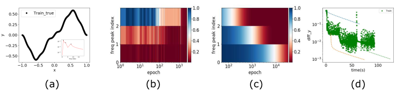
Figure 12: Poisson’s equation. (a) $u_{\mathrm{ref}}(x)$. Inset: $|\hat{u}_{\mathrm{ref}}(k)|$ as a function of frequency. Frequencies peaks are marked with black dots. (b,c) $\Delta_{F}(k)$ computed on the inputs of training data at different epochs for the selected frequencies for DNN (b) and Jacobi (c). (d) $\|h-u_{\mathrm{ref}}\|_{\infty}$ at different running time. Green stars indicate $\|h-u_{\mathrm{ref}}\|_{\infty}$ using DNN alone. The dashed lines indicate $\|h-u_{\mathrm{ref}}\|_{\infty}$ for the Jacobi method with different colors indicating initialization by different timing of DNN training. Xu et al. (2020) use a DNN with widths 1-4000-500-400-1 and full batch training by Adam optimizer Kingma and Ba (2014). The learning rate is $0.0005$. $\beta$ is $10$. The parameters of the DNN are initialized following a Gaussian distribution with mean $0$ and standard deviation $0.02$. Reprinted from Xu et al. (2020).

5.2.2 Ritz-Galerkin (R-G) method

Wang et al. (2020a) study the difference between R-G method and DNN methods, reviewed as follows.

R-G method.

We briefly introduce the R-G method (Brenner and Scott, 2008). For problem (38), we construct a functional

$$J(u)=\frac{1}{2}a(u,u)-(g,u),$$ (51)

where

$$a(u,v)=\int_{\Omega}\nabla u(\bm{x})\nabla v(\bm{x})d\bm{x},\quad(g,v)=\int_{\Omega}g(\bm{x})v(\bm{x})d\bm{x}.$$

The variational form of problem (38) is the following:

$$\text{Find}\;u\in H_{0}^{1}(\Omega),\;\text{s.t.}\;J(u)=\min_{v\in H_{0}^{1}(\Omega)}J(v).$$ (52)

The weak form of (52) is to find $u\in H_{0}^{1}(\Omega)$ such that

$$a(u,v)=(g,v),\quad\forall\;v\in H_{0}^{1}(\Omega).$$ (53)

The problem (38) is the strong form if the solution $u\in H_{0}^{2}(\Omega)$. To numerically solve (53), we now introduce the finite dimensional space $U_{h}$ to approximate the infinite dimensional space $H_{0}^{1}(\Omega)$. Let $U_{h}\subset H_{0}^{1}(\Omega)$ be a subspace with a sequence of basis functions $\{\phi_{1},\phi_{2},\cdots,\phi_{m}\}$. The numerical solution $u_{h}\in U_{h}$ that we will find can be represented as

$$u_{h}=\sum_{k=1}^{m}c_{k}\phi_{k},$$ (54)

where the coefficients $\{c_{i}\}$ are the unknown values that we need to solve. Replacing $H_{0}^{1}(\Omega)$ by $U_{h}$, both problems (52) and (53) can be transformed to solve the following system:

$$\sum_{k=1}^{m}c_{k}a(\phi_{k},\phi_{j})=(g,\phi_{j}),\quad j=1,2,\cdots,m.$$ (55)

From (55), we can calculate $c_{i}$, and then obtain the numerical solution $u_{h}$. We usually call (55) R-G equation.

For different types of basis functions, the R-G method can be divided into finite element method (FEM) and spectral method (SM) and so on. If the basis functions $\{\phi_{i}(\bm{x})\}$ are local, namely, they are compactly supported, this method is usually taken as the FEM. Assume that $\Omega$ is a polygon, and we divide it into finite element grid $\mathcal{T}_{h}$ by simplex, $h=\max_{\tau\in\mathcal{T}_{h}}\text{diam}(\tau)$. A typical finite element basis is the linear hat basis function, satisfying

$$\phi_{k}(\bm{x_{j}})=\delta_{kj},\quad\bm{x_{j}}\in\mathcal{N}_{h},$$ (56)

where $\mathcal{N}_{h}$ stands for the set of the nodes of grid $\mathcal{T}_{h}$. The schematic diagram of the basis functions in 1-D and 2-D are shown in Fig. 13. On the other hand, if we choose the global basis function such as Fourier basis or Legendre basis (Shen et al., 2011), we call R-G method spectral method.

Figure 13: The finite element basis function in 1d and 2d. Reprinted from Wang et al. (2020a).

The error estimate theory of R-G method has been well established. Under suitable assumption on the regularity of solution, the linear finite element solution $u_{h}$ has the following error estimate

$$\|u-u_{h}\|_{1}\leq C_{1}h\|u\|_{2},$$

where the constant $C_{1}$ is independent of grid size $h$. The spectral method has the following error estimate

$$\|u-u_{h}\|\leq\frac{C_{2}}{m^{s}},$$

where $C_{2}$ is a constant and the exponent $s$ depends only on the regularity (smoothness) of the solution $u$. If $u$ is smooth enough and satisfies certain boundary conditions, the spectral method has the spectral accuracy.

Different learning results.

DNNs with ReLU activation function can be proved to be equivalent with a finite element methods in the sense of approximation (He et al., 2018). However, the learning results have a stark difference. To investigate the difference, we utilize a control experiment, that is, solving PDEs given $n$ sample points and controlling the number of bases in R-G method and the number of neurons in DNN equal $m$. Although not realistic in the common usage of R-G method, we choose the case $m>n$ because the two methods are completely different in such situation especially when $m\rightarrow\infty$. Then replacing the integral on the r.h.s. of (55) with the form of MC integral formula, we obtain

$$\sum_{k=1}^{m}c_{k}a(\phi_{k},\phi_{j})=\frac{1}{n}\sum_{i=1}^{n}g(\bm{x}_{i})\phi_{j}(\bm{x}_{i}),\quad j=1,2,\cdots,m.$$ (57)

We consider the 2D case

$$\left\{\begin{array}[]{c}-\Delta u(\bm{x})=g(\bm{x}),\quad\bm{x}\in(0,1)^{2},\\ u(\bm{x})=0,\quad\bm{x}\in\partial(0,1)^{2},\end{array}\right.$$

where $\bm{x}=(x,y)$ and we know the values of $g$ at $n=5^{2}$ points sampled from the function $g(\bm{x}):=g(x,y)=2\pi^{2}\sin(\pi x)\sin(\pi y).$ For a large $m$, Fig. 14 (a,b) plot the R-G solutions with Legendre basis and piecewise linear basis function. It can be seen that the numerical solution is a function with strong singularity. However, Fig. 14(c,d) show that the two-layer DNN solutions are stable without singularity for large $m$.

The smooth solution of DNN, especially when neuron number is large, can be understood through the low-frequency bias, such as the analysis shown in the LFP theory. This helps understand the wide application of DNN in solving PDEs. For example, the low-frequency bias intuitively explains why DNN solve a shock wave by a smooth solution in Michoski et al. (2019).

For R-G method, the following theorem explains why there is singularity in the 2d case when $m$ is large.

Theorem 1.

When $m\rightarrow\infty$, the numerical method (57) is solving the problem

$$\left\{\begin{array}[]{c}\displaystyle-\Delta u(\bm{x})=\frac{1}{n}\sum_{i=1}^{n}\delta(\bm{x}-\bm{x}_{i})g(\bm{x}_{i}),\quad\bm{x}\in\Omega,\\ u(\bm{x})=0,\quad\bm{x}\in\partial\Omega,\end{array}\right.$$ (61)

where $\delta(x)$ represents the Dirac delta function.

This theorem shows that if we consider an over-parameterized FEM, it solves the green function of the PDE. In Poisson’s problem, the 2D Green function has singularity, thus, leading to singular solution. However, for DNN, due to the F-Principle of low-frequency preference, the solution is always relative smooth. Although there exists equivalence between DNN-based algorithm and conventional methods for solving PDEs in the sense of approximation, it is important to take the implicit bias when analyzing the learning results of DNNs.

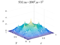
(a) SM

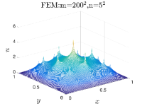
(b) FEM

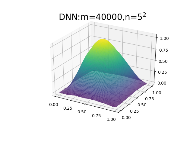
(c) ReLU-DNN

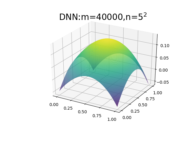
(d) Sin-DNN

Figure 14: R-G solutions (a,b) and two-layer DNN solutions (c,d). Reprinted from Wang et al. (2020a).

5.3 Understanding F-Principle by comparing the differential operator and the integrator operator

In this part, inspired by the analysis in (E et al., 2020) we use a very non-rigorous derivation to intuitively understand why DNN follows the F-Principle while Jacobi method not and shows a connection between these two methods.

Consider the elliptic equation in $1-d$ :

$$\left\{\begin{array}[]{l}Lu:=-\Delta u=g\quad g\in L^{2}([0,1])\\ u(0)=0\\ u(1)=0\end{array}\right.$$

Suppose that $g$ is sufficiently smooth and thus $u$ is smooth, $N>>1,h=1/N,x_{i}=ih=\frac{i}{N},i=0,\ldots,N$.
Let

$$\bm{v}=\left(\begin{array}[]{l}v_{0}\\ v_{1}\\ \vdots\\ v_{N}\end{array}\right)=\left(\begin{array}[]{l}u(0)\\ u(h)\\ \vdots\\ u(1)\end{array}\right),$$

$v_{0}=v_{N}=0$, we have

$$\left(A_{N}\bm{v}\right)_{i}=\frac{1}{h^{2}}\left(-v_{i-1}+2v_{i}-v_{i+1}\right)=g_{i},i=1,\ldots,N-1$$

$$A_{N}\bm{v}=\frac{1}{h^{2}}\left(\begin{array}[]{ccccc}2&-1&&&\\ -1&2&-1&&\\ &-1&\ddots&\ddots&\\ &&\ddots&\ddots&-1\\ &&&-1&2\end{array}\right)\left(\begin{array}[]{l}v_{1}\\ v_{2}\\ \vdots\\ v_{N-1}\end{array}\right)$$

$k=1,\cdots,N-1$ (mode) , $i=1,\cdots,N-1$, which can be extended to $i=0,N$ by considering the boundary conditions.

Define $\left(\bm{w}_{k}\right)_{i}:=\sin\frac{ik\pi}{N},\left(\bm{w}_{k}\right)_{0}:=\left(\bm{w}_{k}\right)_{N}:=0,$

$$\left(A_{N}\bm{w}_{k}\right)_{i} =\frac{1}{h^{2}}\left(-\left(\bm{w}_{k}\right)_{i-1}+2\left(\bm{w}_{k}\right)_{i}-\left(\bm{w}_{k}\right)_{i+1}\right)$$

$$=\frac{1}{h^{2}}\left(-\sin\frac{(i-1)k\pi}{N}+2\sin\frac{ik\pi}{N}-\sin\frac{(i+1)k\pi}{N}\right)$$

$$=\frac{1}{h^{2}}\left(-2\sin\frac{ik\pi}{N}\cos\frac{k\pi}{N}+2\sin\frac{ik\pi}{N}\right)$$

$$=\left(\bm{w}_{k}\right)_{i}\frac{2}{h^{2}}\left(1-\cos\frac{k\pi}{N}\right)$$

$$=\frac{4}{h^{2}}\sin^{2}\frac{k\pi}{2N}\left(\bm{\omega}_{k}\right)_{i}\quad i=1,\cdots,N-1$$

Thus we have

$$A_{N}\bm{w}_{k}=\lambda_{k}\bm{w}_{k},$$

where $\lambda_{k}=\frac{4}{h^{2}}\sin^{2}\frac{k\pi}{N}k=1,\cdots,N-1$.

As the analysis in Jacobi iteration in Section 5.2.1, for differential operator $A_{N}$, lower frequency converges more slowly. This can also be revealed by optimizing $\bm{v}$ through a mean square error as follows. Define $\bm{e}=\bm{v}-\bm{u}^{*}$ as the error on the discretized grid points, and

$$R_{A}:=\frac{1}{2N}\left\|A_{N}\bm{v}-g\right\|^{2},$$

By gradient descent flow, we have

$$\begin{aligned} \frac{d}{dt}\bm{v}=&-\nabla_{\bm{v}}R_{A}\\ =&-\frac{1}{N}A_{N}\left(A_{N}\bm{v}-\bm{g}\right)\end{aligned},$$

then,

$$\begin{aligned} \frac{d}{dt}\bm{e}=-\frac{1}{N}A_{N}^{2}\bm{e}\end{aligned}.$$

Similarly, we obtain that low frequency converges more slowly.

Then, we consider $u(\bm{x};\bm{\theta})$ be the NN function parameterized by $\bm{\theta}$ to approximate the PDE solution. The loss function is similarly defined,

$$\begin{aligned} R_{N}:&=\frac{1}{2N}\sum_{i=1}^{N-1}\left(\left(A_{N}u\right)\left(x_{i},\bm{\theta}\right)-g\left(x_{i}\right)\right)^{2}+\frac{1}{2}u\left(x_{0},\bm{\theta}\right)^{2}+\frac{1}{2}u\left(x_{N},\bm{\theta}\right)^{2}\\ &=\frac{1}{2N}\left\|A_{N}u-g\right\|^{2}+\frac{1}{2}u\left(x_{0},\bm{\theta}\right)^{2}+\frac{1}{2}u\left(x_{N},\bm{\theta}\right)^{2}\end{aligned},$$

The gradient flow w.r.t. $\bm{\theta}$ is

$$\dot{\bm{\theta}}=-\nabla_{\bm{\theta}}R_{N}(\bm{\theta}).$$

Then, the evolution of $u(\bm{x},\bm{\theta})$ is

$$\begin{aligned} \frac{d}{dt}u\left(x_{i},\bm{\theta}\right)=&-\nabla_{\bm{\theta}}u\left(x_{i},\bm{\theta}\right)\cdot\nabla_{\bm{\theta}}R_{N}(\bm{\theta})\\ =&-\nabla_{\bm{\theta}}u\left(x_{i},\bm{\theta}\right)\left[\frac{1}{N}\sum_{j=1}^{N-1}\left(\left(A_{N}^{2}u\right)_{j}-\left(A_{N}g\right)_{j}\right)\nabla_{\bm{\theta}}u\left(x_{j},\bm{\theta}\right)\right.\\ &\left.+u\left(x_{0},\bm{\theta}\right)\nabla_{\bm{\theta}}u\left(x_{0},\bm{\theta}\right)+u\left(x_{N},\bm{\theta}\right)\nabla_{\bm{\theta}}u\left(x_{N},\bm{\theta}\right)\right]\\ =&-\frac{1}{N}\sum_{j=1}^{N-1}K\left(x_{i},x_{j}\right)\left(\left(A_{N}^{2}u\right)_{j}-\left(A_{N}g\right)_{j}\right)\\ &-K\left(x_{i},x_{0}\right)u\left(x_{0}\right)-K\left(x_{i},x_{N}\right)u\left(x_{N}\right)\end{aligned},$$

where $K:=\left(K\left(x_{i},x_{j}\right)\right)_{(N-1)\times(N-1)}=\left(\nabla_{\bm{\theta}}u\left(x_{i},\bm{\theta}\right)\cdot\nabla_{\bm{\theta}}u\left(x_{j},\bm{\theta}\right)\right)_{(N-1)\times(N-1)}$ is the spectrum defined in Section 3.3.1.

We similarly define the error as $e:=u-u^{*}$. Then,

$$\frac{d}{dt}e\left(x_{i},\bm{\theta}\right)= -\frac{1}{N}\left[\sum_{i=1}^{N-1}K\left(x_{i},x_{j}\right)\left(A_{N}^{2}e\right)_{j}\right.$$

$$\left.-NK\left(x_{i},x_{0}\right)e_{0}-NK\left(x_{i},x_{N}\right)e_{N}\right]$$

where $K=\left(K\left(x_{i},x_{j}\right)\right),i,j=0,\cdots,N.$ Define $\bar{e}=(e_{0},\cdots,e_{N})$ and consider the augmented matrix:

$$\bar{A}_{N}\bar{\bm{v}}=\frac{1}{h^{2}}\left(\begin{array}[]{ccccccc}C\\ &2&-1&&&\\ &-1&2&-1&&\\ &&-1&\ddots&\ddots&\\ &&&\ddots&\ddots&-1\\ &&&&-1&2\\ &&&&&&C\end{array}\right)\left(\begin{array}[]{l}v_{0}\\ v_{1}\\ \vdots\\ v_{N}\end{array}\right).$$

where $C$ is to be determined. For $j=1,\cdots,N-1$, $\left.\bar{A}_{N}^{2}\bar{\bm{e}}\right|_{j}=\left.A_{N}^{2}\bm{e}\right|_{j}$, for $j=0$,

$$\left.\bar{A}_{N}^{2}\bar{e}\right|_{0}=\left(\frac{C}{h^{2}}\right)^{2}e_{0}=Ne_{0}\Leftrightarrow\frac{C}{h^{2}}=\sqrt{N}$$

$$C=h^{2}\frac{1}{\sqrt{h}}=h^{3/2}$$

Taken together, we have

$$\frac{d}{dt}\bar{e}=-\frac{1}{N}K\bar{A}_{N}^{2}\bar{e}.$$ (62)

Although for differential operator (derivative w.r.t. input), lower-frequency mode converges more slowly, for integral operator (loss consists of the summation w.r.t. input), i.e., spectrum $K$, lower-frequency mode (see Section 3.3) converges faster. Therefore, there is a competition between $K$ and $A_{N}$, which is the competition between integral and differential operators (also see analysis in E et al. (2020)). The effect of neural network can also be understood as a preconditioner. Another easy way to understand why differential operator enables faster convergence of high frequency is that the Fourier transform of $\nabla u(x)$ is $\xi\hat{u}(\xi)$, that is, a higher frequency would have a higher weight in the loss function.

5.4 Algorithm design to overcome the curse of high-frequency

The F-Principle provides valuable theoretical insights of the limit of DNN-based algorithms, that is, the curse of high-frequency (Xu et al., 2020).

To overcome the curse of high-frequency in DNN-based algorithms, a series of methods are proposed. Jagtap et al. (2020) replace the activation function $\sigma(x)$ by a $\sigma(\mu ax)$, where $\mu$ is a fixed scale factor with $\mu\geq 1$ and $a$ is a trainable variable shared for all neurons. Biland et al. (2019) explicitly impose high frequencies with higher priority in the loss function to accelerate the simulation of fluid dynamics. PhaseDNN Cai et al. (2020) convert high frequency component of the data downward to a low frequency spectrum for learning, and then convert the learned one back to original high frequency. Another way to understand PhaseDNN is that expanding the target function by a Fourier series, due to the cut-off of high-frequency, the coefficient should slightly depend on the input, i.e., coefficients should be low-frequency functions and easy to be learned by DNNs. Peng et al. (2020) call the used basis of Fourier expansion as prior dictionaries. Such approach is effective in low-dimensional problems. However, due to the number of Fourier terms exponentially increases with the dimension, the PhaseDNN would suffer from the curse of dimensionality.

To alleviate the effect of high dimension, a Multi-scale DNN (MscaleDNN) method, originally proposed in Cai and Xu (2019) and completed in Liu et al. (2020), considers the frequency conversion only in the radial direction. Li et al. (2020c, 2021) further improve the design of MscaleDNN. This can also similarly be understood by the Fourier expansion but only in the radial direction. The conversion in the frequency space can be done by a scaling, which is equivalent to a inverse scaling in the spatial space. Therefore, we can use the following ansatz to fit high-frequency data

$$f(\bm{x})\sim{\displaystyle\sum\limits_{i=1}^{M}}f_{\theta^{n_{i}}}(\alpha_{i}\bm{x}).$$ (63)

This can be easily implemented by multiplying the input to different neurons in the first hidden layer with different constant scalings. Fig. 15 shows two examples of MscaleDNN structures. Wang et al. (2020b); Li et al. (2020c, 2021) further use MscaleDNN to solve more multi-scale problems. Another key factor in practical experiments, without too much understanding, is the effect of activation function. Liu et al. (2020) use activation functions with compact support. Huang et al. (2021); Li et al. (2021) adopt the MscaleDNN structure and use the sine and cosine functions as the activation function with different scalings for neurons in the first hidden layer and obtain better results in solving PDEs. The MscaleDNN structure is now widely applied in alleviating the curse of high frequency Ying et al. (2022).

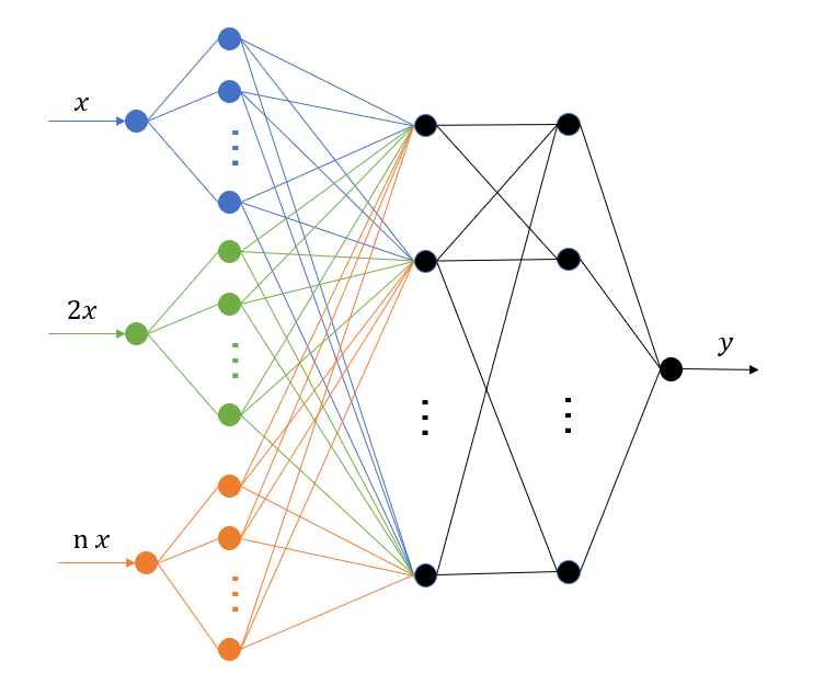
(a) MscaleDNN-1

(b) MscaleDNN-2

Figure 15: Illustration of two MscaleDNN structures. Reprinted from Liu et al. (2020).

6 Application of the F-Principle

The study of the F-Principle has been utilized to understand various phenomena emerging in applications of deep learning and to inspire the design of DNN-based algorithms. In this section, we briefly review some applications of the F-Principle, but not a complete list.

6.1 Frequency perspective for understanding experimental phenomena

Compression phase.

Xu et al. (2019) explain the compression phase in information plane, proposed by Shwartz-Ziv and Tishby (2017), by the F-Principle as follows. The entropy or information quantifies the possibility of output values, i.e., more possible output values leads to a higher entropy. In learning a discretized function, the DNN first fits the continuous low-frequency components of the discretized function, i.e., large entropy state. Then, the DNN output tends to be discretized as the network gradually captures the high-frequency components, i.e., entropy decreasing. Thus, the compression phase appears in the information plane.

Increasing complexity.

The F-Principle also explains the increasing complexity of DNN output during the training. For common small initialization, the initial output of a DNN is often close to zero. The F-Principle indicates that the output of DNN contains higher and higher frequency during the training. As frequency is a natural concept to characterize the complexity of a function, the F-Principle indicates that the complexity of the DNN output increases during the training. This increasing complexity of DNN output during training is consistent with previous studies and subsequent works (Arpit et al., 2017; Kalimeris et al., 2019; Goldt et al., 2020; He et al., 2020; Mingard et al., 2019; Jin et al., 2020).

Strength and limitation.

Ma et al. (2020) show that the F-Principle may be a general mechanism behind the slow deterioration phenomenon in the training of DNNs, where the effect of the “double descent” is washed out. Sharma and Ross (2020) utilize the low-frequency bias of DNNs to study effectiveness of an iris recognition DNN. Chen et al. (2019) show that under the same computational budget, a MuffNet is a better universal approximator for functions containing high frequency components, thus, better for mobile deep learning. Zhu et al. (2019) utilize the F-Principle to help understand why high frequency is a limit when DNNs is used to solve spectral deconvolution problem. Chakrabarty (2019) utilize the idea of F-Principle to study the spectral bias of the deep image prior.

Deep frequency principle.

Xu and Zhou (2021) propose a deep frequency principle to understand an effect of depth in accelerating the training. For a DNN, the effective target function of the $l$-th hidden layer can be understood in the following way. Its input is the output of the $(l-1)$-th layer. The part from the $l$-th layer is to learn the mapping from the output of the $(l-1)$-th layer to the true labels. Therefore, the effective target function of the $l$-th hidden layer consists of the output of the $(l-1)$-th layer and the true labels. Xu and Zhou (2021) empirically find a deep frequency principle: The effective target function for a deeper hidden layer biases towards lower frequency during the training. Due to the F-Principle, this empirical study provides a rationale for understanding why depth can accelerate the training.

Frequency approach.

Camuto et al. (2020) show that the effect of Gaussian noise injections to each hidden layer output is equivalent to a penalty of high-frequency components in the Fourier domain. Rabinowitz (2019); Deng and Zhang (2021) use the F-Principle as one of typical phenomena to study the difference between the normal learning and the meta-learning. Chen et al. (2021b) show the frequency principle holds in a broad learning system. Schwarz et al. (2021) study the frequency bias of generative models.

6.2 Inspiring the design of algorithm

In addition to scientific computing reviewed in section 5.4, to accelerate the convergence of high-frequency, different approaches are developed in various applications. Some examples are listed in the following.

Jagtap et al. (2020); Agarwal et al. (2020); Liang et al. (2021) design different types of activation functions. Campo et al. (2020) use a frequency filter to help reduce the interdependency between the low frequency and the (harder to learn) high frequency components of the state-action value approximation to achieve better results in reinforcement learning. Several works use multi-scale input by projecting data into a high dimensional space with a set of sinusoids in efficiently representing complex 3D objects and scenes. (Tancik et al., 2020; Mildenhall et al., 2020; Bi et al., 2020; Pumarola et al., 2021; Hennigh et al., 2021; Wang et al., 2021; Xu et al., 2021; Häni et al., 2020; Zheng et al., 2020; Peng et al., 2021; Guo et al., 2020). Tancik et al. (2021) use meta-learning to obtain a good initialization for fast and effective image restoration. Several works utilize frequency-aware information to improve the quality of high-frequency details of images generated by neural networks Chen et al. (2021a); Jiang et al. (2020); Yang et al. (2022); Li et al. (2022). Xi et al. (2020) argue that the performance improvement in low-resolution image classification is affected by the inconsistency of the information loss and learning priority on low-frequency components and high-frequency components, and propose a network structure to overcome this inconsistent issue.

The F-Principle shows that DNNs quickly learn the low-frequency part, which is often dominated in the real data and more robust. At the early stage, the DNN is similar to a linear model (Kalimeris et al., 2019; Hu et al., 2020). Some works take advantage of DNN at early training stage to save training computation cost. The original lottery ticket network (Frankle and Carbin, 2018) requires a full training of DNN, which has a very high computational cost. Most computation is used to capture high frequency while high frequency may be not important in many cases. You et al. (2020) show that a small but critical subnetwork emerge at the early training stage (Early-Bird ticket), and the performance of training this small subnetwork with the same initialization is similar to the training of the full network, thus, saving significant energy for training networks. Fu et al. (2021, 2020) utilize the robust of low frequency by applying low-precision for early training stage to save computational cost without sacrificing the generalization performance.

7 Anti-F-Principle

F-Principle is rather common in training DNNs. As we have understood F-Principle to a certain extent, it is also easy to construct examples in which F-Principle does not hold, i.e., anti-F-Principle. As analyzed in Section 3.3.3, if the priority of high frequency is too high, the optimization problem would lead to trivial solutions. Examples in overparameterized finite element method in Fig. 14 is also an example. In this section, we review some anti-F-Principle examples.

7.1 Derivative w.r.t. input

Imposing high priority on high frequency can alleviate the effect of the F-Principle and sometimes an anti-F-Principle can be observed. Similar to Section 5.3, if the loss function contains the gradient of the DNN output w.r.t. the input, it is equivalent to impose higher frequency with higher weight in the loss function. Then, whether there exists a F-Principle depends on the competition between the activation regularity and the loss function. If the loss function endorses more priority for the high frequency to compensate the low-priority induced by the activation function, an anti-F-Principle emerges. Since gradient often exists in solving PDEs, the anti-F-Principle can be observed in solving a PDE by designing a loss with high-order derivatives. Some analysis and numerical experiments can also be found in Lu et al. (2021b); E et al. (2020).

7.2 Large weights

Another way to observe anti-F-Principle is using large values for network weights. As shown in the analysis of idealized setting in Sec. 3.1, large weights alleviate the dominance of low-frequency in Eq. (9). In addition, large values would also cause large fluctuation of DNN output at initialization (experiments can be seen in Xu et al. (2019)), the amplitude term in Eq. (9) may endorse high frequency larger priority, leading to an anti-F-Principle, which is also studied in Yang and Salman (2019). In the NTK regime (Jacot et al., 2018), Zhang et al. (2020) theoretically show that the fluctuation of the initial output would be kept in the learned function after training.

8 Conclusion

F-Principle is very general and important for training DNNs. It serves as a basic principle to understand DNNs and to inspire the design of DNNs. As a good starting point, F-Principle leads to more interesting studies for better understanding DNNs. For examples, Empirical study also find the F-Principle holds in non-gradient training process Ma et al. (2021). It remains unclear how to build a theory of F-Principle for general DNNs with arbitrary sample distribution and study the generalization error. The precise description of F-Principle is only done in the NTK regime (Jacot et al., 2018), it is not clear whether it is possible to obtain a similarly precise description in the mean-field regime described by partial differential equations (Mei et al., 2018; Sirignano and Spiliopoulos, 2020; Rotskoff and Vanden-Eijnden, 2018). The Fourier analysis can be used to study DNNs from other perspectives, such as the effect of different image frequency on the learning results.

As a general implicit bias, F-Principle is insufficient to characterize the exact details of the training process of DNNs beyond NTK. To study the nonlinear behavior of DNNs in detail, it is important to study DNNs from other perspectives, such as the loss landscape, the effect of width and depth, the effect of initialization, etc. For example, Zhang et al. (2020); Luo et al. (2021b) have studied how initialization affects the implicit bias of DNNs and (Luo et al., 2021b) draw a phase diagram for wide two-layer ReLU DNNs (Luo et al., 2021b). Zhang et al. (2021c, d) show an embedding principle that the loss landscape of a DNN “contains” all the critical points of all the narrower DNNs.

References

- Xu et al. (2019) Zhi-Qin J Xu, Yaoyu Zhang, and Yanyang Xiao. Training behavior of deep neural network in frequency domain. International Conference on Neural Information Processing, pages 264–274, 2019.
- Xu et al. (2020) Zhi-Qin John Xu, Yaoyu Zhang, Tao Luo, Yanyang Xiao, and Zheng Ma. Frequency principle: Fourier analysis sheds light on deep neural networks. Communications in Computational Physics, 28(5):1746–1767, 2020.
- Rahaman et al. (2019) Nasim Rahaman, Devansh Arpit, Aristide Baratin, Felix Draxler, Min Lin, Fred A Hamprecht, Yoshua Bengio, and Aaron Courville. On the spectral bias of deep neural networks. International Conference on Machine Learning, 2019.
- Zhang et al. (2021a) Yaoyu Zhang, Tao Luo, Zheng Ma, and Zhi-Qin John Xu. A linear frequency principle model to understand the absence of overfitting in neural networks. Chinese Physics Letters, 38(3):038701, 2021a.
- Liu et al. (2020) Ziqi Liu, Wei Cai, and Zhi-Qin John Xu. Multi-scale deep neural network (mscalednn) for solving poisson-boltzmann equation in complex domains. Communications in Computational Physics, 28(5):1970–2001, 2020.
- Jagtap et al. (2020) Ameya D Jagtap, Kenji Kawaguchi, and George Em Karniadakis. Adaptive activation functions accelerate convergence in deep and physics-informed neural networks. Journal of Computational Physics, 404:109136, 2020.
- Cai et al. (2020) Wei Cai, Xiaoguang Li, and Lizuo Liu. A phase shift deep neural network for high frequency approximation and wave problems. SIAM Journal on Scientific Computing, 42(5):A3285–A3312, 2020.
- Tancik et al. (2020) Matthew Tancik, Pratul Srinivasan, Ben Mildenhall, Sara Fridovich-Keil, Nithin Raghavan, Utkarsh Singhal, Ravi Ramamoorthi, Jonathan Barron, and Ren Ng. Fourier features let networks learn high frequency functions in low dimensional domains. In Advances in Neural Information Processing Systems, volume 33, pages 7537–7547. Curran Associates, Inc., 2020.
- Breiman (1995) Leo Breiman. Reflections after refereeing papers for nips. The Mathematics of Generalization, XX:11–15, 1995.
- Zhang et al. (2017) Chiyuan Zhang, Samy Bengio, Moritz Hardt, Benjamin Recht, and Oriol Vinyals. Understanding deep learning requires rethinking generalization. In 5th International Conference on Learning Representations, ICLR 2017, Toulon, France, April 24-26, 2017, Conference Track Proceedings. OpenReview.net, 2017.
- Dyson (2004) Freeman Dyson. A meeting with Enrico Fermi. Nature, 427(6972):297–297, 2004.
- Simonyan and Zisserman (2015) Karen Simonyan and Andrew Zisserman. Very deep convolutional networks for large-scale image recognition. In 3rd International Conference on Learning Representations, ICLR 2015, San Diego, CA, USA, May 7-9, 2015, Conference Track Proceedings, 2015.
- Brown et al. (2020) Tom B Brown, Benjamin Mann, Nick Ryder, Melanie Subbiah, Jared Kaplan, Prafulla Dhariwal, Arvind Neelakantan, Pranav Shyam, Girish Sastry, Amanda Askell, et al. Language models are few-shot learners. arXiv preprint arXiv:2005.14165, 2020.
- Jiang et al. (2019) Yiding Jiang, Behnam Neyshabur, Hossein Mobahi, Dilip Krishnan, and Samy Bengio. Fantastic generalization measures and where to find them. In International Conference on Learning Representations, 2019.
- Saxe et al. (2014) Andrew M. Saxe, James L. McClelland, and Surya Ganguli. Exact solutions to the nonlinear dynamics of learning in deep linear neural networks. In The International Conference on Learning Representations, 2014.
- Saxe et al. (2019) Andrew M. Saxe, Yamini Bansal, Joel Dapello, Madhu Advani, Artemy Kolchinsky, Brendan D. Tracey, and David D. Cox. On the information bottleneck theory of deep learning. Journal of Statistical Mechanics: Theory and Experiment, 2019(12):124020, 2019. doi: 10.1088/1742-5468/ab3985.
- Lampinen and Ganguli (2019) Andrew K. Lampinen and Surya Ganguli. An analytic theory of generalization dynamics and transfer learning in deep linear networks. In The International Conference on Learning Representations, 2019.
- Engel and Broeck (2001) A. Engel and C. Van den Broeck. Statistical Mechanics of Learning. 2001. Google-Books-ID: qVo4IT9ByfQC.
- Aubin et al. (2018) Benjamin Aubin, Antoine Maillard, jean barbier, Florent Krzakala, Nicolas Macris, and Lenka Zdeborová. The committee machine: Computational to statistical gaps in learning a two-layers neural network. In Advances in Neural Information Processing Systems 31, pages 3223–3234. 2018.
- Choromanska et al. (2015) Anna Choromanska, Mikael Henaff, Michael Mathieu, Gérard Ben Arous, and Yann LeCun. The loss surfaces of multilayer networks. In Artificial Intelligence and Statistics, pages 192–204, 2015.
- Mei et al. (2018) Song Mei, Andrea Montanari, and Phan-Minh Nguyen. A mean field view of the landscape of two-layer neural networks. Proceedings of the National Academy of Sciences, 115(33):E7665–E7671, 2018.
- Rotskoff and Vanden-Eijnden (2018) Grant M Rotskoff and Eric Vanden-Eijnden. Parameters as interacting particles: long time convergence and asymptotic error scaling of neural networks. In Proceedings of the 32nd International Conference on Neural Information Processing Systems, pages 7146–7155, 2018.
- Chizat and Bach (2018) Lénaïc Chizat and Francis Bach. On the global convergence of gradient descent for over-parameterized models using optimal transport. Advances in Neural Information Processing Systems, 31:3036–3046, 2018.
- Sirignano and Spiliopoulos (2020) Justin Sirignano and Konstantinos Spiliopoulos. Mean field analysis of neural networks: A central limit theorem. Stochastic Processes and their Applications, 130(3):1820–1852, 2020.
- Jacot et al. (2018) Arthur Jacot, Franck Gabriel, and Clément Hongler. Neural tangent kernel: convergence and generalization in neural networks. In Proceedings of the 32nd International Conference on Neural Information Processing Systems, pages 8580–8589, 2018.
- Lee et al. (2019) Jaehoon Lee, Lechao Xiao, Samuel Schoenholz, Yasaman Bahri, Roman Novak, Jascha Sohl-Dickstein, and Jeffrey Pennington. Wide Neural Networks of Any Depth Evolve as Linear Models Under Gradient Descent. In Advances in Neural Information Processing Systems 32, pages 8572–8583. 2019.
- Zdeborová (2020) Lenka Zdeborová. Understanding deep learning is also a job for physicists. Nature Physics, 16:1–3, 2020. ISSN 1745-2481. doi: 10.1038/s41567-020-0929-2.
- Luo et al. (2021a) Tao Luo, Zheng Ma, Zhi-Qin John Xu, and Yaoyu Zhang. Theory of the frequency principle for general deep neural networks. CSIAM Transactions on Applied Mathematics, 2(3):484–507, 2021a. ISSN 2708-0579. doi: https://doi.org/10.4208/csiam-am.SO-2020-0005.
- Zhang et al. (2019) Yaoyu Zhang, Zhi-Qin John Xu, Tao Luo, and Zheng Ma. Explicitizing an implicit bias of the frequency principle in two-layer neural networks. arXiv preprint arXiv:1905.10264, 2019.
- Luo et al. (2020a) Tao Luo, Zheng Ma, Zhi-Qin John Xu, and Yaoyu Zhang. On the exact computation of linear frequency principle dynamics and its generalization. arXiv preprint arXiv:2010.08153, 2020a.
- Cao et al. (2021) Yuan Cao, Zhiying Fang, Yue Wu, Ding-Xuan Zhou, and Quanquan Gu. Towards understanding the spectral bias of deep learning. In Proceedings of the Thirtieth International Joint Conference on Artificial Intelligence, IJCAI-21, pages 2205–2211, 8 2021.
- Yang and Salman (2019) Greg Yang and Hadi Salman. A fine-grained spectral perspective on neural networks. arXiv preprint arXiv:1907.10599, 2019.
- Ronen et al. (2019) Basri Ronen, David Jacobs, Yoni Kasten, and Shira Kritchman. The convergence rate of neural networks for learned functions of different frequencies. Advances in Neural Information Processing Systems, 32:4761–4771, 2019.
- Bordelon et al. (2020) Blake Bordelon, Abdulkadir Canatar, and Cengiz Pehlevan. Spectrum dependent learning curves in kernel regression and wide neural networks. In International Conference on Machine Learning, pages 1024–1034. PMLR, 2020.
- E et al. (2020) Weinan E, Chao Ma, and Lei Wu. Machine learning from a continuous viewpoint, i. Science China Mathematics, pages 1–34, 2020.
- Giryes and Bruna (2020) Raja Giryes and Joan Bruna. How can we use tools from signal processing to understand better neural networks? Inside Signal Processing Newsletter, 2020.
- Arpit et al. (2017) Devansh Arpit, Stanisław Jastrzębski, Nicolas Ballas, David Krueger, Emmanuel Bengio, Maxinder S Kanwal, Tegan Maharaj, Asja Fischer, Aaron Courville, Yoshua Bengio, et al. A closer look at memorization in deep networks. In International Conference on Machine Learning, pages 233–242. PMLR, 2017.
- Chen et al. (2021a) Yuanqi Chen, Ge Li, Cece Jin, Shan Liu, and Thomas Li. Ssd-gan: Measuring the realness in the spatial and spectral domains. In Proceedings of the AAAI Conference on Artificial Intelligence, volume 35, pages 1105–1112, 2021a.
- Jiang et al. (2020) Liming Jiang, Bo Dai, Wayne Wu, and Chen Change Loy. Focal frequency loss for generative models. arXiv preprint arXiv:2012.12821, 2020.
- Xi et al. (2020) Yue Xi, Wenjing Jia, Jiangbin Zheng, Xiaochen Fan, Yefan Xie, Jinchang Ren, and Xiangjian He. Drl-gan: Dual-stream representation learning gan for low-resolution image classification in uav applications. IEEE Journal of selected topics in applied earth observations and remote sensing, 14:1705–1716, 2020.
- Xu (2018) Zhiqin John Xu. Understanding training and generalization in deep learning by fourier analysis. arXiv preprint arXiv:1808.04295, 2018.
- Xie et al. (2017) Bo Xie, Yingyu Liang, and Le Song. Diverse neural network learns true target functions. In Proceedings of the 20th International Conference on Artificial Intelligence and Statistics, AISTATS 2017, 20-22 April 2017, Fort Lauderdale, FL, USA, volume 54 of Proceedings of Machine Learning Research, pages 1216–1224. PMLR, 2017.
- Basri et al. (2020) Ronen Basri, Meirav Galun, Amnon Geifman, David Jacobs, Yoni Kasten, and Shira Kritchman. Frequency bias in neural networks for input of non-uniform density. In International Conference on Machine Learning, pages 685–694. PMLR, 2020.
- Dong et al. (2019) Bin Dong, Jikai Hou, Yiping Lu, and Zhihua Zhang. Distillation early stopping? harvesting dark knowledge utilizing anisotropic information retrieval for overparameterized neural network. arXiv preprint arXiv:1910.01255, 2019.
- Kopitkov and Indelman (2020) Dmitry Kopitkov and Vadim Indelman. Neural spectrum alignment: Empirical study. In International Conference on Artificial Neural Networks, pages 168–179. Springer, 2020.
- Baratin et al. (2020) Aristide Baratin, Thomas George, César Laurent, R Devon Hjelm, Guillaume Lajoie, Pascal Vincent, and Simon Lacoste-Julien. Implicit regularization via neural feature alignment. arXiv preprint arXiv:2008.00938, 2020.
- Luo et al. (2020b) Tao Luo, Zheng Ma, Zhi-Qin John Xu, and Yaoyu Zhang. On the exact computation of linear frequency principle dynamics and its generalization. arXiv preprint arXiv:2010.08153, 2020b.
- Jin and Montúfar (2020) Hui Jin and Guido Montúfar. Implicit bias of gradient descent for mean squared error regression with wide neural networks. arXiv preprint arXiv:2006.07356, 2020.
- Luo et al. (2020c) Tao Luo, Zheng Ma, Zhiwei Wang, Zhi-Qin John Xu, and Yaoyu Zhang. Fourier-domain variational formulation and its well-posedness for supervised learning. arXiv preprint arXiv:2012.03238, 2020c.
- Shalev-Shwartz et al. (2017) Shai Shalev-Shwartz, Ohad Shamir, and Shaked Shammah. Failures of gradient-based deep learning. In International Conference on Machine Learning, pages 3067–3075. PMLR, 2017.
- Nye and Saxe (2018) Maxwell Nye and Andrew Saxe. Are efficient deep representations learnable? arXiv preprint arXiv:1807.06399, 2018.
- Lin et al. (2016) Junhong Lin, Raffaello Camoriano, and Lorenzo Rosasco. Generalization properties and implicit regularization for multiple passes sgm. In International Conference on Machine Learning, pages 2340–2348. PMLR, 2016.
- Li et al. (2020a) Mingchen Li, Mahdi Soltanolkotabi, and Samet Oymak. Gradient descent with early stopping is provably robust to label noise for overparameterized neural networks. In International conference on artificial intelligence and statistics, pages 4313–4324. PMLR, 2020a.
- E et al. (2019) Weinan E, Chao Ma, and Lei Wu. A Priori Estimates of the Population Risk for Two-layer Neural Networks. Communications in Mathematical Sciences, 17(5):1407–1425, 2019. doi: 10.4310/CMS.2019.v17.n5.a11.
- Arora et al. (2019) Sanjeev Arora, Simon Du, Wei Hu, Zhiyuan Li, and Ruosong Wang. Fine-grained analysis of optimization and generalization for overparameterized two-layer neural networks. In International Conference on Machine Learning, pages 322–332. PMLR, 2019.
- Ma et al. (2020) Chao Ma, Lei Wu, and E Weinan. The slow deterioration of the generalization error of the random feature model. In Mathematical and Scientific Machine Learning, pages 373–389. PMLR, 2020.
- E et al. (2017) Weinan E, Jiequn Han, and Arnulf Jentzen. Deep learning-based numerical methods for high-dimensional parabolic partial differential equations and backward stochastic differential equations. Communications in Mathematics and Statistics, 5(4):349–380, 2017.
- Khoo and Ying (2019) Yuehaw Khoo and Lexing Ying. Switchnet: a neural network model for forward and inverse scattering problems. SIAM Journal on Scientific Computing, 41(5):A3182–A3201, 2019.
- He et al. (2018) Juncai He, Lin Li, Jinchao Xu, and Chunyue Zheng. Relu deep neural networks and linear finite elements. arXiv preprint arXiv:1807.03973, 2018.
- Fan et al. (2019) Yuwei Fan, Lin Lin, Lexing Ying, and Leonardo Zepeda-Núnez. A multiscale neural network based on hierarchical matrices. Multiscale Modeling & Simulation, 17(4):1189–1213, 2019.
- Han et al. (2019) Jiequn Han, Chao Ma, Zheng Ma, and E Weinan. Uniformly accurate machine learning-based hydrodynamic models for kinetic equations. Proceedings of the National Academy of Sciences, 116(44):21983–21991, 2019.
- Weinan et al. (2018) E Weinan, Chao Ma, and Jianchun Wang. Model reduction with memory and the machine learning of dynamical systems. Communications in Computational Physics, 25(4):947–962, 2018. ISSN 1991-7120.
- He and Xu (2019) Juncai He and Jinchao Xu. Mgnet: A unified framework of multigrid and convolutional neural network. Science china mathematics, 62(7):1331–1354, 2019.
- Strofer et al. (2019) Carlos Michelen Strofer, Jin-Long Wu, Heng Xiao, and Eric Paterson. Data-driven, physics-based feature extraction from fluid flow fields using convolutional neural networks. Communications in Computational Physics, 25(3):625–650, 2019.
- Han et al. (2018) Jiequn Han, Linfeng Zhang, Roberto Car, et al. Deep potential: A general representation of a many-body potential energy surface. Communications in Computational Physics, 23(3), 2018.
- Dissanayake and Phan-Thien (1994) MWMG Dissanayake and Nhan Phan-Thien. Neural-network-based approximations for solving partial differential equations. communications in Numerical Methods in Engineering, 10(3):195–201, 1994.
- Raissi et al. (2019) Maziar Raissi, Paris Perdikaris, and George E Karniadakis. Physics-informed neural networks: A deep learning framework for solving forward and inverse problems involving nonlinear partial differential equations. Journal of Computational Physics, 378:686–707, 2019.
- Zang et al. (2020) Yaohua Zang, Gang Bao, Xiaojing Ye, and Haomin Zhou. Weak adversarial networks for high-dimensional partial differential equations. Journal of Computational Physics, 411:109409, 2020.
- Li et al. (2020b) Zongyi Li, Nikola Kovachki, Kamyar Azizzadenesheli, Burigede Liu, Kaushik Bhattacharya, Andrew Stuart, and Anima Anandkumar. Fourier neural operator for parametric partial differential equations. arXiv preprint arXiv:2010.08895, 2020b.
- Lu et al. (2021a) Lu Lu, Pengzhan Jin, Guofei Pang, Zhongqiang Zhang, and George Em Karniadakis. Learning nonlinear operators via deeponet based on the universal approximation theorem of operators. Nature Machine Intelligence, 3(3):218–229, 2021a.
- Zhang et al. (2021b) Lulu Zhang, Tao Luo, Yaoyu Zhang, Zhi-Qin John Xu, and Zheng Ma. Mod-net: A machine learning approach via model-operator-data network for solving pdes. arXiv preprint arXiv:2107.03673, 2021b.
- E et al. (2021) Weinan E, Jiequn Han, and Arnulf Jentzen. Algorithms for solving high dimensional pdes: From nonlinear monte carlo to machine learning. Nonlinearity, 35(1):278, 2021.
- Evans (2010) Lawrence C Evans. Partial differential equations. 2010.
- E and Yu (2018) Weinan E and Bing Yu. The deep ritz method: A deep learning-based numerical algorithm for solving variational problems. Communications in Mathematics and Statistics, 6(1):1–12, 2018.
- Huang et al. (2020) Jianguo Huang, Haoqin Wang, and Haizhao Yang. Int-deep: A deep learning initialized iterative method for nonlinear problems. Journal of Computational Physics, 419:109675, 2020.
- Kingma and Ba (2014) Diederik P Kingma and Jimmy Ba. Adam: A method for stochastic optimization. arXiv preprint arXiv:1412.6980, 2014.
- Wang et al. (2020a) Jihong Wang, Zhi-Qin John Xu, Jiwei Zhang, and Yaoyu Zhang. Implicit bias with ritz-galerkin method in understanding deep learning for solving pdes. arXiv preprint arXiv:2002.07989, 2020a.
- Brenner and Scott (2008) Susanne C Brenner and L. Ridgway Scott. The mathematical theory of finite element methods. Springer, New York, third edition, 2008.
- Shen et al. (2011) Jie Shen, Tao Tang, and Li Lian Wang. Spectral methods. Algorithms, analysis and applications. Springer, 2011.
- Michoski et al. (2019) Craig Michoski, Milos Milosavljevic, Todd Oliver, and David Hatch. Solving irregular and data-enriched differential equations using deep neural networks. arXiv preprint arXiv:1905.04351, 2019.
- Biland et al. (2019) Simon Biland, Vinicius C Azevedo, Byungsoo Kim, and Barbara Solenthaler. Frequency-aware reconstruction of fluid simulations with generative networks. arXiv preprint arXiv:1912.08776, 2019.
- Peng et al. (2020) Wei Peng, Weien Zhou, Jun Zhang, and Wen Yao. Accelerating physics-informed neural network training with prior dictionaries. arXiv preprint arXiv:2004.08151, 2020.
- Cai and Xu (2019) Wei Cai and Zhi-Qin John Xu. Multi-scale deep neural networks for solving high dimensional pdes. arXiv preprint arXiv:1910.11710, 2019.
- Li et al. (2020c) Xi-An Li, Zhi-Qin John Xu, and Lei Zhang. A multi-scale dnn algorithm for nonlinear elliptic equations with multiple scales. Communications in Computational Physics, 28(5):1886–1906, 2020c.
- Li et al. (2021) Xi-An Li, Zhi-Qin John Xu, and Lei Zhang. Subspace decomposition based dnn algorithm for elliptic-type multi-scale pdes. arXiv preprint arXiv:2112.06660, 2021.
- Wang et al. (2020b) Bo Wang, Wenzhong Zhang, and Wei Cai. Multi-scale deep neural network (mscalednn) methods for oscillatory stokes flows in complex domains. Communications in Computational Physics, 28(5):2139–2157, 2020b.
- Huang et al. (2021) Xiang Huang, Hongsheng Liu, Beiji Shi, Zidong Wang, Kang Yang, Yang Li, Bingya Weng, Min Wang, Haotian Chu, Jing Zhou, Fan Yu, Bei Hua, Lei Chen, and Bin Dong. Solving partial differential equations with point source based on physics-informed neural networks. arXiv preprint arXiv:2111.01394, 2021.
- Ying et al. (2022) Jinyong Ying, Jiaxuan Liu, Jiaxin Chen, Sen Cao, Muzhou Hou, and Yinghao Chen. Multi-scale fusion network: a new deep learning structure for elliptic interface problems. Applied Mathematical Modelling, 2022.
- Shwartz-Ziv and Tishby (2017) Ravid Shwartz-Ziv and Naftali Tishby. Opening the black box of deep neural networks via information. arXiv preprint arXiv:1703.00810, 2017.
- Kalimeris et al. (2019) Dimitris Kalimeris, Gal Kaplun, Preetum Nakkiran, Benjamin Edelman, Tristan Yang, Boaz Barak, and Haofeng Zhang. Sgd on neural networks learns functions of increasing complexity. Advances in Neural Information Processing Systems, 32:3496–3506, 2019.
- Goldt et al. (2020) Sebastian Goldt, Marc Mézard, Florent Krzakala, and Lenka Zdeborová. Modeling the influence of data structure on learning in neural networks: The hidden manifold model. Physical Review X, 10(4):041044, 2020.
- He et al. (2020) Shilin He, Xing Wang, Shuming Shi, Michael R Lyu, and Zhaopeng Tu. Assessing the bilingual knowledge learned by neural machine translation models. arXiv preprint arXiv:2004.13270, 2020.
- Mingard et al. (2019) Chris Mingard, Joar Skalse, Guillermo Valle-Pérez, David Martínez-Rubio, Vladimir Mikulik, and Ard A Louis. Neural networks are a priori biased towards boolean functions with low entropy. arXiv preprint arXiv:1909.11522, 2019.
- Jin et al. (2020) Pengzhan Jin, Lu Lu, Yifa Tang, and George Em Karniadakis. Quantifying the generalization error in deep learning in terms of data distribution and neural network smoothness. Neural Networks, 130:85–99, 2020.
- Sharma and Ross (2020) Renu Sharma and Arun Ross. D-netpad: An explainable and interpretable iris presentation attack detector. In 2020 IEEE International Joint Conference on Biometrics (IJCB), pages 1–10. IEEE, 2020.
- Chen et al. (2019) Hesen Chen, Ming Lin, Xiuyu Sun, Qian Qi, Hao Li, and Rong Jin. Muffnet: Multi-layer feature federation for mobile deep learning. In Proceedings of the IEEE/CVF International Conference on Computer Vision Workshops, pages 0–0, 2019.
- Zhu et al. (2019) Hu Zhu, Yiming Qiao, Guoxia Xu, Lizhen Deng, and Yu Yu-Feng. Dspnet: A lightweight dilated convolution neural networks for spectral deconvolution with self-paced learning. IEEE Transactions on Industrial Informatics, 2019.
- Chakrabarty (2019) Prithvijit Chakrabarty. The spectral bias of the deep image prior. In Bayesian Deep Learning Workshop and Advances in Neural Information Processing Systems (NeurIPS), 2019.
- Xu and Zhou (2021) Zhi-Qin John Xu and Hanxu Zhou. Deep frequency principle towards understanding why deeper learning is faster. In Proceedings of the AAAI Conference on Artificial Intelligence, volume 35, 2021.
- Camuto et al. (2020) Alexander Camuto, Matthew Willetts, Umut Şimşekli, Stephen Roberts, and Chris Holmes. Explicit regularisation in gaussian noise injections. arXiv preprint arXiv:2007.07368, 2020.
- Rabinowitz (2019) Neil C Rabinowitz. Meta-learners’ learning dynamics are unlike learners’. arXiv preprint arXiv:1905.01320, 2019.
- Deng and Zhang (2021) Xiang Deng and Zhongfei Mark Zhang. Is the meta-learning idea able to improve the generalization of deep neural networks on the standard supervised learning? In 2020 25th International Conference on Pattern Recognition (ICPR), pages 150–157. IEEE, 2021.
- Chen et al. (2021b) Guang-Yong Chen, Min Gan, CL Philip Chen, Hong-Tao Zhu, and Long Chen. Frequency principle in broad learning system. IEEE Transactions on Neural Networks and Learning Systems, 2021b.
- Schwarz et al. (2021) Katja Schwarz, Yiyi Liao, and Andreas Geiger. On the frequency bias of generative models. Advances in Neural Information Processing Systems, 34, 2021.
- Agarwal et al. (2020) Rishabh Agarwal, Nicholas Frosst, Xuezhou Zhang, Rich Caruana, and Geoffrey E Hinton. Neural additive models: Interpretable machine learning with neural nets. arXiv preprint arXiv:2004.13912, 2020.
- Liang et al. (2021) Senwei Liang, Liyao Lyu, Chunmei Wang, and Haizhao Yang. Reproducing activation function for deep learning. arXiv preprint arXiv:2101.04844, 2021.
- Campo et al. (2020) Miguel Campo, Zhengxing Chen, Luke Kung, Kittipat Virochsiri, and Jianyu Wang. Band-limited soft actor critic model. arXiv preprint arXiv:2006.11431, 2020.
- Mildenhall et al. (2020) Ben Mildenhall, Pratul P Srinivasan, Matthew Tancik, Jonathan T Barron, Ravi Ramamoorthi, and Ren Ng. Nerf: Representing scenes as neural radiance fields for view synthesis. In European Conference on Computer Vision, pages 405–421. Springer, 2020.
- Bi et al. (2020) Sai Bi, Zexiang Xu, Pratul Srinivasan, Ben Mildenhall, Kalyan Sunkavalli, Miloš Hašan, Yannick Hold-Geoffroy, David Kriegman, and Ravi Ramamoorthi. Neural reflectance fields for appearance acquisition. arXiv preprint arXiv:2008.03824, 2020.
- Pumarola et al. (2021) Albert Pumarola, Enric Corona, Gerard Pons-Moll, and Francesc Moreno-Noguer. D-nerf: Neural radiance fields for dynamic scenes. In Proceedings of the IEEE/CVF Conference on Computer Vision and Pattern Recognition, pages 10318–10327, 2021.
- Hennigh et al. (2021) Oliver Hennigh, Susheela Narasimhan, Mohammad Amin Nabian, Akshay Subramaniam, Kaustubh Tangsali, Zhiwei Fang, Max Rietmann, Wonmin Byeon, and Sanjay Choudhry. Nvidia simnet: An ai-accelerated multi-physics simulation framework. In International Conference on Computational Science, pages 447–461. Springer, 2021.
- Wang et al. (2021) Sifan Wang, Hanwen Wang, and Paris Perdikaris. On the eigenvector bias of fourier feature networks: From regression to solving multi-scale pdes with physics-informed neural networks. Computer Methods in Applied Mechanics and Engineering, 384:113938, 2021.
- Xu et al. (2021) Rui Xu, Xintao Wang, Kai Chen, Bolei Zhou, and Chen Change Loy. Positional encoding as spatial inductive bias in gans. In Proceedings of the IEEE/CVF Conference on Computer Vision and Pattern Recognition, pages 13569–13578, 2021.
- Häni et al. (2020) Nicolai Häni, Selim Engin, Jun-Jee Chao, and Volkan Isler. Continuous object representation networks: novel view synthesis without target view supervision. arXiv preprint arXiv:2007.15627, 2020.
- Zheng et al. (2020) Quan Zheng, Vahid Babaei, Gordon Wetzstein, Hans-Peter Seidel, Matthias Zwicker, and Gurprit Singh. Neural light field 3d printing. ACM Transactions on Graphics (TOG), 39(6):1–12, 2020.
- Peng et al. (2021) Sida Peng, Yuanqing Zhang, Yinghao Xu, Qianqian Wang, Qing Shuai, Hujun Bao, and Xiaowei Zhou. Neural body: Implicit neural representations with structured latent codes for novel view synthesis of dynamic humans. In Proceedings of the IEEE/CVF Conference on Computer Vision and Pattern Recognition, pages 9054–9063, 2021.
- Guo et al. (2020) Michelle Guo, Alireza Fathi, Jiajun Wu, and Thomas Funkhouser. Object-centric neural scene rendering. arXiv preprint arXiv:2012.08503, 2020.
- Tancik et al. (2021) Matthew Tancik, Ben Mildenhall, Terrance Wang, Divi Schmidt, Pratul P Srinivasan, Jonathan T Barron, and Ren Ng. Learned initializations for optimizing coordinate-based neural representations. In Proceedings of the IEEE/CVF Conference on Computer Vision and Pattern Recognition, pages 2846–2855, 2021.
- Yang et al. (2022) Mengping Yang, Zhe Wang, Ziqiu Chi, and Yanbing Zhang. Fregan: Exploiting frequency components for training gans under limited data. arXiv preprint arXiv:2210.05461, 2022.
- Li et al. (2022) Yanyan Li, Weilong Peng, Keke Tang, and Meie Fang. Spatio-frequency decoupled weak-supervision for face reconstruction. Computational Intelligence & Neuroscience, 2022.
- Hu et al. (2020) Wei Hu, Lechao Xiao, Ben Adlam, and Jeffrey Pennington. The surprising simplicity of the early-time learning dynamics of neural networks. arXiv preprint arXiv:2006.14599, 2020.
- Frankle and Carbin (2018) Jonathan Frankle and Michael Carbin. The lottery ticket hypothesis: Finding sparse, trainable neural networks. arXiv preprint arXiv:1803.03635, 2018.
- You et al. (2020) Haoran You, Chaojian Li, Pengfei Xu, Yonggan Fu, Yue Wang, Xiaohan Chen, Yingyan Lin, Zhangyang Wang, and Richard G Baraniuk. Drawing early-bird tickets: Towards more efficient training of deep networks. International Conference on Learning Representations, 2020.
- Fu et al. (2021) Yonggan Fu, Han Guo, Meng Li, Xin Yang, Yining Ding, Vikas Chandra, and Yingyan Lin. CPT: Efficient Deep Neural Network Training via Cyclic Precision. arXiv:2101.09868, January 2021.
- Fu et al. (2020) Yonggan Fu, Haoran You, Yang Zhao, Yue Wang, Chaojian Li, Kailash Gopalakrishnan, Zhangyang Wang, and Yingyan Lin. Fractrain: Fractionally squeezing bit savings both temporally and spatially for efficient DNN training. In Advances in Neural Information Processing Systems 33: Annual Conference on Neural Information Processing Systems 2020, NeurIPS 2020, December 6-12, 2020, virtual, 2020.
- Lu et al. (2021b) Lu Lu, Xuhui Meng, Zhiping Mao, and George Em Karniadakis. Deepxde: A deep learning library for solving differential equations. SIAM Review, 63(1):208–228, 2021b.
- Zhang et al. (2020) Yaoyu Zhang, Zhi-Qin John Xu, Tao Luo, and Zheng Ma. A type of generalization error induced by initialization in deep neural networks. In Mathematical and Scientific Machine Learning, pages 144–164. PMLR, 2020.
- Ma et al. (2021) Yuheng Ma, Zhi-Qin John Xu, and Jiwei Zhang. Frequency principle in deep learning beyond gradient-descent-based training. arXiv preprint arXiv:2101.00747, 2021.
- Luo et al. (2021b) Tao Luo, Zhi-Qin John Xu, Zheng Ma, and Yaoyu Zhang. Phase diagram for two-layer relu neural networks at infinite-width limit. Journal of Machine Learning Research, 22:1–47, 2021b.
- Zhang et al. (2021c) Yaoyu Zhang, Zhongwang Zhang, Tao Luo, and Zhi-Qin John Xu. Embedding principle of loss landscape of deep neural networks. NeurIPS, 2021c.
- Zhang et al. (2021d) Yaoyu Zhang, Yuqing Li, Zhongwang Zhang, Tao Luo, and Zhi-Qin John Xu. Embedding principle: a hierarchical structure of loss landscape of deep neural networks. arXiv preprint arXiv:2111.15527, 2021d.