An Optimization Framework for General Rate Splitting for General Multicast
Abstract
Immersive video, such as virtual reality (VR) and multi-view videos, is growing in popularity. Its wireless streaming is an instance of general multicast, extending conventional unicast and multicast, whose effective design is still open. This paper investigates general rate splitting for general multicast. Specifically, we consider a multi-carrier single-cell wireless network where a multi-antenna base station (BS) communicates to multiple single-antenna users via general multicast. We consider linear beamforming at the BS and joint decoding at each user in the slow fading and fast fading scenarios. In the slow fading scenario, we consider the maximization of the weighted sum average rate, which is a challenging nonconvex stochastic problem with numerous variables. To reduce computational complexity, we decouple the original nonconvex stochastic problem into multiple nonconvex deterministic problems, one for each system channel state. Then, we propose an iterative algorithm for each deterministic problem to obtain a Karush-Kuhn-Tucker (KKT) point using the concave-convex procedure (CCCP). In the fast fading scenario, we consider the maximization of the weighted sum ergodic rate. This problem is more challenging than the one for the slow fading scenario, as it is not separable. First, we propose a stochastic iterative algorithm to obtain a KKT point using stochastic successive convex approximation (SSCA) and the exact penalty method. Then, we propose two low-complexity iterative algorithms to obtain feasible points with promising performance for two cases of channel distributions using approximation and CCCP. The proposed optimization framework generalizes the existing ones for rate splitting for various types of services. Finally, we numerically show substantial gains of the proposed solutions over existing schemes in both scenarios and reveal the design insights of general rate splitting for general multicast.
Index Terms:
General multicast, general rate splitting, linear beamforming, joint decoding, optimization, concave-convex procedure (CCCP), stochastic successive convex approximation (SSCA).I Introduction
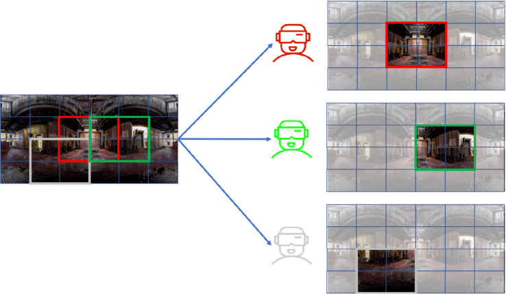
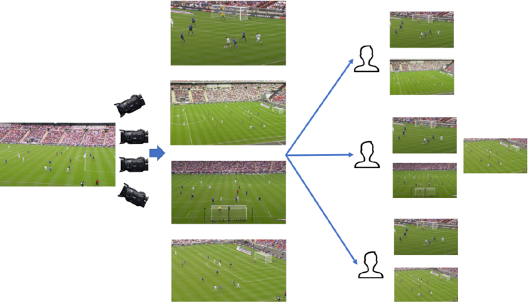
Conventional mobile Internet services include (traditional) video, audio, web browsing, social networking, software downloading, etc. These services can be supported by unicast, unicast with a common message, single-group multicast, and multi-group multicast. Immersive video, such as 360 video (projection of virtual reality (VR) spherical video onto a rectangle) and multi-view video (a key technique in free-viewpoint television, naked-eye 3D and VR), is growing in popularity. It is predicted that the VR market will reach 87.97 billion USD by 2025[1]. When watching a 360 video, the tiles in a user’s current FoV plus a safe margin are usually transmitted to the user in case of FoV change. On the other hand, when watching a multi-view video, a user’s current view and adjacent views are usually transmitted to the user in case of a view switch. In wireless streaming of a popular immersive video to multiple users simultaneously, multiple messages (e.g., tiles for 360 video and views for multi-view video) are transmitted to each user, and one message may be intended for multiple users[2, 3], as illustrated in Fig. 1. This emerging service plays an important role in online gaming, self-driving, and cloud meeting, etc. but cannot perfectly adapt to the conventional transmission schemes mentioned above. This motivates us to consider general multicast (also referred to as general connection[7, 8] and general groupcast [9]) where one message can be intended for any user. Clearly, general multicast includes conventional unicast, unicast with a common message, single-group multicast, and multi-group multicast as special cases.
References[2, 3, 4, 5] are pioneer works for supporting wireless streaming of a 360 video[2, 4] and wireless streaming of a multi-view video[3, 5], which are instances of general multicast. In [2, 3, 4, 5], Orthogonal Multiple Access (OMA), such as Time Division Multiple Access (TDMA)[2, 3] and Orthogonal Frequency Division Multiple Access (OFDMA)[4, 5], is adopted to convert general multicast to per resource block single-group multicast. While the OMA-based mechanisms are easy to implement, spatial multiplexing gain is not exploited. On the other hand, non-orthogonal transmission mechanisms achieve higher transmission efficiency but are also more challenging due to interference. Space Division Multiple Access (SDMA) and Non-Orthogonal Multiple Access (NOMA) are two solutions. The cost to suppress interference in SDMA can be high when the channels for some users are spatially aligned, while decoding interference in NOMA may not be possible when the interfering message rate is too high. Thus, SDMA and NOMA may have unsatisfactory performance. Rate splitting[6, 20] is introduced to partially suppress interference and partially decode interference to circumvent these limitations.
Rate splitting is originally proposed to effectively support unicast services[12]. Specifically, [12] investigates the simplest form of rate splitting for unicast, hereafter called 1-layer rate splitting, for the two-user interference channel. The idea of 1-layer rate splitting is as follows. First, each individual message is split into one private part and one common part, respectively. Then, the common parts of all the messages are re-assembled into one common message that is multicasted to all the users, and the private parts are unicasted to the corresponding receivers, respectively. In this way, part of the interference can be removed since it is decodable by design. Later, in [13], 1-layer rate splitting is applied to the multi-antenna broadcast channel (BC) and shown to provide a strict sum degree of freedom gain of a BC when only imperfect channel state information at the transmitter is available. In [14, 15, 16, 17, 18], the authors investigate the precoder optimization of 1-layer rate splitting for unicast for Gaussian multiple-input multiple-output channels. In particular, the rates and beamforming vectors for common and private messages are optimized to maximize the sum rate[14, 18], worst-case rate[15, 16] or ergodic sum rate[17]. On the one hand, [19, 20] extend 1-layer rate splitting for unicast to general rate splitting for unicast and study the optimization of three-user unicast[19] and multi-user unicast[20], respectively, with linear precoding. On the other hand, [21, 22, 23, 24, 25] generalize 1-layer rate splitting for unicast to 1-layer rate splitting for unicast together with a multicast message intended for all users [21] and multi-group multicast[22, 23, 24, 25], respectively, and investigate the optimizations with linear beamforming. Note that most works[14, 15, 16, 18, 19, 20, 21, 23, 24, 25] focus on the slow fading scenario, whereas [17],[22] concentrates on the fast fading scenario.
Optimization-based random linear network coding designs for general multicast have been studied in [7, 8] for wired networks. Besides, general rate splitting for general multicast has been studied in [9] for discrete memoryless broadcast channels. Here, we are interested in Gaussian fading channels and specifically the linear beamforming design from the optimization perspective. In general rate splitting for general multicast, each message intended for a user group is split into sub-messages, one for each subset of users containing the user group. Then, the sub-messages intended for the same group of users are re-assembled and multicasted to the group. In this way, each user group decodes the desired message and part of the message of any other user group. Note that general rate splitting for general multicast produces more sub-messages and enables more flexible and effective interference reduction than brute-force application of general rate splitting for unicast[19, 20] to general multicast.111One can brute-forcely apply general rate splitting[19, 20] for unicast to general multicast by treating a group of users who request the same message as a virtual user. Besides, the optimizations of rate splitting for unicast and its slight generalization in [21, 22, 23, 24, 25] cannot apply to general multicast. Therefore, for general multicast in both slow fading and fast fading scenarios, the optimization of general rate splitting with linear beamforming remains an open problem.
This paper intends to shed some light on the above issue. Specifically, we consider a multi-carrier single-cell wireless network, where a multi-antenna base station (BS) communicates to multiple single-antenna users via general multicast. Our main contributions are summarized below.
-
•
We present general rate splitting for general multicast and illustrate its connection with conventional unicast, unicast with a common message, single-group multicast, and multi-group multicast. We adopt linear beamforming at the BS and joint decoding at each user and characterize the corresponding rate regions in the slow fading and fast fading scenarios.
-
•
In the slow fading scenario, we optimize the transmission beamforming vectors and rates of sub-message units to maximize the weighted sum average rate. Note that the proposed problem formulation can reduce to those for general rate splitting for unicast[20], unicast with a common message[21], single-group multicast[26], and 1-layer rate splitting for multi-group multicast[23]. This problem is a challenging nonconvex stochastic problem with a large number of variables. To reduce computational complexity, we decouple the original nonconvex stochastic problem into multiple nonconvex deterministic problems, one for each system channel state. Then, for each nonconvex deterministic problem, we propose an iterative algorithm to obtain a Karush-Kuhn-Tucker (KKT) point using the concave-convex procedure (CCCP).
-
•
In the fast fading scenario, we optimize the transmission beamforming vectors and rates of sub-message units to maximize the weighted sum ergodic rate and show that the problem formulation can reduce to the one for 1-layer rate splitting for unicast[17]. This problem is more challenging than the one for the slow fading scenario, as it is not separable. First, we propose a stochastic iterative algorithm to obtain a KKT point using stochastic successive convex approximation (SSCA) and the exact penalty method. Then, we propose two low-complexity iterative algorithms to obtain feasible points with promising performance for two cases of channel distributions, i.e., spatially correlated channel and independent and identically distributed (i.i.d.) channel, using approximation and CCCP. It is noteworthy that the proposed optimization framework also provides general rate splitting designs for other service types in the fast fading scenario.
-
•
We compare the complexities of the proposed solutions in the slow fading and fast fading scenarios. We also numerically demonstrate substantial gains of the proposed solutions over existing schemes in both scenarios and reveal the design insights of general rate splitting for general multicast.
| Notation | Description |
| number of users | |
| set of user indices | |
| number of messages | |
| set of the indices of messages | |
| set of the indices of messages requested by user | |
| subset of | |
| set of the indices of the messages requested by each user in and not requested by any user in | |
| subsets of that contain | |
| rate of the message unit | |
| rate of the message unit under | |
| number of the antennas | |
| number of the subcarriers | |
| bandwidth of each subcarrier | |
| beamforming vector for transmitting on subcarrier under | |
| constant beamforming vector for transmitting on subcarrier |
Notation: We represent vectors by boldface lowercase letters (e.g., ), matrices by boldface uppercase letters (e.g., ), scalar constants by non-boldface letters (e.g., ), sets by calligraphic letters (e.g., ), and sets of sets by boldface calligraphic letters (e.g., ). The notation represents the -th element of vector . The symbol denotes complex conjugate transpose operator. denotes the Euclidean norm of a vector. denotes the real part of a complex number. denotes the statistical expectation. denotes the identity matrix. denotes the set of complex numbers.
II System Model
In this section, we first introduce general multicast in a single-cell wireless network and briefly illustrate its connection with unicast, unicast with a common message, single-group multicast, and multi-group multicast. Then, we present the physical layer model and general rate splitting with joint decoding for general multicast. The key notation used in this paper is listed in Table I.
II-A General Multicast
We consider a single-cell wireless network consisting of one BS and users. Let denote the set of user indices. The BS has independent messages. Let denote the set of the indices of messages. We consider general multicast. Specifically, each user can request arbitrary messages in , denoted by , from the BS. We do not have any assumptions on except that each message in is requested by at least one user, i.e., .
To facilitate serving the users, we partition the message set according to the requests from the users. For all , let
| (1) |
denote the set of the indices of messages requested by each user in and not requested by any user in [2]. Define
Thus, forms a partition of and specifies the user groups corresponding to the partition. We refer to each element in as a message unit.222 and are assumed to be given in [9]. We can see that different message units in are requested by different user groups in .
Example 1 (Illustration of and for Two-User Case)
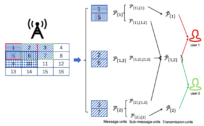
As illustrated in Fig. 2 (a), we consider , , , . Then, we have , , , , and . There are 3 message units that are requested by 3 groups of users, respectively. For example, message unit is requested only by user 1 and message unit is requested by user 1 and user 2.333This general multicast scenario coincides with unicast with a common message.
Example 2 (Illustration of and for Three-User Case)
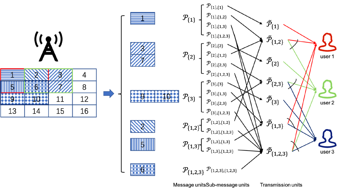
As illustrated in Fig. 2 (b), we consider , , , , . Then, we have , , , , , , , and . There are 6 message units that are requested by 6 groups of users, respectively. For example, message unit is requested only by user 1, message unit is requested by user 1 and user 2, and message unit is requested by user 1, user 2, and user 3.
Remark 1 (Connection with Unicast and Multicast)
The considered general multicast includes conventional unicast, unicast with a common message, single-group multicast, and multi-group multicast as special cases. (i) When , and , general multicast reduces to unicast[14, 15, 16, 17, 18, 19, 20]. In this case, and . (ii) When , and , general multicast reduces to unicast with a common message[21]. In this case, and . (iii) When , implying , and , general multicast becomes single-group multicast[26]. In this case, and . (iv) When and , general multicast reduces to multi-group (-group) multicast[22, 23, 24, 25]. In this case, and . The general multicast considered in this paper, general connection in [7, 8], and general groupcast considered in [9] mean the same.
II-B General Rate Splitting
We consider rate splitting in the most general form for general multicast to serve the users[9]. It allows each user group to decode not only the desired message unit but also part of the message unit of any other user group, for all , to flexibly reduce the interference level. For all , let . Namely, collects all subsets of that contain . Define . Obviously, . First, we split each message unit into sub-message units. Accordingly, the rate of the message unit , denoted by , is split into the rates of the sub-message units, denoted by 444When , and the message unit will not be split. For ease of exposition, we let for . i.e.,
| (2) |
Let . Then, for all , we re-assemble the sub-message units to form a transmission unit with rate:
| (3) |
That is, we first split message units, , into sub-message units and then we re-assemble these sub-message units to form transmission units, .
Example 3 (Illustration of and General Rate Splitting for Two-User Case)
For Example 1, we have , , . As shown in Fig. 2 (a), we first split 3 message units into 5 sub-message units and then re-assemble the 5 sub-message units to form 3 transmission units.
Example 4 (Illustration of and General Rate Splitting for Three-User Case)
For Example 2, we have , , , , , . As shown in Fig. 2 (b), we first split 6 message units into 17 sub-message units and then re-assemble the 17 sub-message units to form 7 transmission units.
Remark 2 (Connection with Rate Splitting for Unicast and Multicast)
(i) When general multicast degrades to unicast, the proposed general rate splitting reduces to the general rate splitting for unicast proposed in our previous work [20], which extends the one-layer rate splitting for unicast [17]. (ii) When general multicast degrades to unicast with a common message, the proposed general rate splitting reduces to the one-layer rate splitting for unicast with a common message[21]. (iii) When general multicast degrades to single-group multicast, the proposed general rate splitting reduces to the conventional single-group multicast transmission[26]. (iv) When general multicast degrades to multi-group multicast, the proposed general rate splitting reduces to the one-layer rate splitting for multi-group multicast [23].
II-C Physical Layer Model
The BS is equipped with antennas, and each user has one antenna. We consider a multi-carrier system. Let and denote the number of subcarriers and the set of subcarrier indices, respectively. The bandwidth of each subcarrier is (in Hz). We consider a discrete-time system, i.e., time is divided into fixed-length slots. We adopt the block fading model, i.e., for each user and subcarrier, the channel remains constant within each slot and is independent and identically distributed (i.i.d.) over slots. Let denote the -dimensional random channel vector for user and subcarrier , where denotes the -dimensional channel state space. Let denote the random system channel state, where represents the system channel state space. Besides, let denote a realization of in one slot, where is a realization of . Assume that user knows his channel state in each slot. We consider two channel models which are presented below.
II-C1 Slow Fading
We assume that the system channel state is known to the BS in each slot and adopt transmission rate adaptation over slots. We consider channel coding within each slot and across the subcarriers. For the sake of exposition, we consider an arbitrary slot with system channel state and any user group . Let denote the component of to be transmitted to user group in the slot, also referred to as message unit, and denote the corresponding (transmission) rate of . Then, the average rate of message unit is given by . We apply the general rate splitting scheme presented in Section II-B to transmit to all user groups in in the slot. Specifically, for all , message unit is split into sub-message units. The rate of and the rates of the sub-message unit, denoted by , satisfy:
| (4) |
Then, for all , we re-assemble sub-message units to form transmission unit with rate:
| (5) |
For all , transmission unit is encoded (channel coding) into codewords that span over the subcarriers. Let denote a symbol for that is transmitted on the -th subcarrier. For all , let , and assume that . We consider linear beamforming. For all , let denote the beamforming vector for transmitting on subcarrier in the slot. Using superposition coding, the transmitted signal on subcarrier , denoted by , is given by:
| (6) |
The transmission power on subcarrier is given by , and the total transmission power is given by . In the slow fading scenario, the total transmission power constraint is given by:
| (7) |
Here, denotes the transmission power budget. Define . Then, the received signal at user on subcarrier , denoted by , is given by:
| (8) |
where the last equality is due to (6), and is the additive white gaussian noise (AWGN). In (8), the first term represents the desired signal, and the second represents the interference. It is noteworthy that the main idea of rate splitting is to make the undesired messages partially decodable in order to reduce interference [20]. To exploit the full potential of the general rate splitting for general multicast, we consider joint decoding at each user.555We can easily extend it to successive decoding as in [20]. That is, each user jointly decodes the desired transmission units . Thus, in the slow fading scenario, the achievable rate region of the transmission units in the slot with system channel state is described by the following constraints:
| (9) |
where is given by (5).
Example 5 (Illustration of Physical Layer Design for Two-user Case in Slow Fading)
For Example 1, the rates of message units , , and are , , and , respectively. The rates of transmission units , , and are , , and , respectively. The beamforming vectors for transmitting , , and on subcarrier are , , and , respectively.
Example 6 (Illustration of Physical Layer Design for Three-user Case in Slow Fading)
For Example 2, the rates of message units , , , , , and are , , , , , and , respectively. The rates of transmission units , , , , , , and are , , , , , , and , respectively. The beamforming vectors for transmitting , , , , , , and on subcarrier are , , , , , , and , respectively.
II-C2 Fast Fading
We assume that the system channel state is unknown to the BS in each slot, but its distribution is known to the BS. We consider channel coding over many slots and across the subcarriers. We apply the general rate splitting scheme presented in Section II-B to transmit to all user groups in over many slots. For all , transmission unit is encoded into codewords that span over the subcarriers and many slots. Let denote a symbol for that is transmitted on the -th subcarrier. Let denote the constant beamforming vector for transmitting on subcarrier over these slots. Similarly, using superposition coding, the transmitted signal on subcarrier is given by:
| (10) |
The total transmission power is given by . In the fast fading scenario, the total transmission power constraint is given by:
| (11) |
Then, in a slot with system channel state , the received signal at user on subcarrier , denoted by , is given by:
where the last equality is due to (10). Similarly, we consider joint decoding at each user. The achievable ergodic rate region of the transmission units over these slots is given by:
| (12) |
where is given by (3).
Example 7 (Illustration of Physical Layer Design for Two-user Case in Fast Fading)
For Example 1, the rates of message units , , and are , , and , respectively. The rates of transmission units , , and are , , and , respectively. The beamforming vectors for transmitting , , and on subcarrier are , , and , respectively.
Example 8 (Illustration of Physical Layer Design for Three-user Case in Fast Fading)
For Example 2, the rates of message units , , , , , and are , , , , , and , respectively. The rates of transmission units , , , , , , and are , , , , , , and , respectively. The beamforming vectors for transmitting , , , , , , and on subcarrier are , , , , , , and , respectively.
III Average Rate Maximization In Slow Fading Scenario
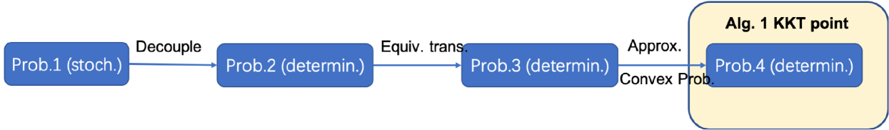
This section considers the slow fading scenario and maximizes the weighted sum average rate under the achievable rate constraints and total transmission power constraints. The proposed solution framework for the slow fading scenario is illustrated in Fig. 3.
III-A Optimization Problem Formulation
We would like to optimize the transmission beamforming vectors and rates of the sub-message units to maximize the weighted sum average rate,666The proposed problem formulation and solution method can be readily extended to maximize the sum average rate and worst-case average rate as in [20]. , where the coefficient denotes the weight for message unit , subject to the total transmission power constraints in (7) and the achievable rate constraints in (9). Therefore, we formulate the following optimization problem.
Problem 1 (Weighted Sum Average Rate Maximization)
where is given by (4).
As the objective function and constraints of Problem 1 are seperable with , Problem 1 is seperable and can be readily solved by solving the following problems for all in parallel.
Problem 2 (Weighted Sum Rate Maximization for )
| (13) | |||
| (14) |
Remark 3 (Connection with Rate Splitting for Unicast and Multicast)
(i) When general multicast degrades to unicast, Problem 2 reduces to the weighted sum rate maximization problem for general rate splitting for unicast in [20]. (ii) When general multicast degrades to unicast with a common message, Problem 2 can be viewed as a generalization of the weighted sum rate maximization for unicast with a common message in [21]. (iii) When general multicast degrades to single-group multicast, Problem 2 reduces to the rate maximization problem for single-group multicast in [26]. (iv) When general multicast degrades to multi-group multicast, Problem 2 can be viewed as a generalization of the weighted sum rate maximization for multi-group multicast in [23].
Therefore, we can focus on solving Problem 2 for all . Note that the objective function is linear, the constraint in (13) is convex, and the constraints in (14) are nonconvex. Thus, Problem 2 is nonconvex.777There are generally no effective methods for solving a nonconvex problem optimally. The goal of solving a nonconvex problem is usually to design an iterative algorithm to obtain a stationary point or a KKT point (which satisfies necessary conditions for optimality if strong duality holds).
III-B KKT Point
In this subsection, we propose an iterative algorithm to obtain a KKT point of Problem 2 using CCCP. First, we transform Problem 2 into the following equivalent problem by introducing auxiliary variables and and extra constraints:
| (15) | |||
| (16) |
| (17) |
Proof 1
First, by introducing auxiliary variables and and extra constraints:
| (18) |
we can equivalently transform Problem 2 into the following problem:
Let denote an optimal solution. It is obvious that is an optimal solution of Problem 2. Next, we transform the above problem to Problem 3 by relaxing the constrains in (18) to the constraints in (16). By contradiction and the monotonicity of the objective function with respect to (w.r.t.) in Problem 3, we can show that the constraints in (16) are active at the optimal solution. Thus, is an optimal solution of Problem 3. Therefore, we can show Lemma 1.
Based on Lemma 1, solving Problem 2 is equivalent to solving Problem 3. Problem 3 is a difference of convex functions (DC) programming (one type of nonconvex problems), and a KKT point can be obtained by CCCP[20].888CCCP can exploit the partial convexity and usually converges faster to a KKT point than conventional gradient methods. The main idea of CCCP is to solve a sequence of successively refined approximate convex problems, each of which is obtained by linearizing the concave part and preserving the remaining convex part in the DC problem. Specifically, at the -th iteration, the approximate convex problem of Problem 3 is given as follows. Let denote an optimal solution of the following problem.
Problem 4 (Approximation of Problem 3 at Iteration )
| (19) |
where , , and
| (20) |
Problem 4 is convex and can be solved efficiently using standard convex optimization methods[28]. Problem 4 has variables and constraints. Thus, when an interior point method is applied, the computational complexity for solving Problem 4 is as [28]. The details of CCCP for obtaining a KKT point of Problem 3 are summarized in Algorithm 1.999In practice, we can run each of Algorithms 1-4 multiple times with randomly selected feasible initial points to obtain multiple KKT points and choose the KKT point with the best objective value. As the number of iterations of Algorithm 1 does not scale with the problem size[29], the computational complexity for Algorithm 1 is the same as that for solving Problem 4, i.e., as .
Theorem 1 (Convergence of Algorithm 1)
Proof 2
The constraints in (13), (15), (16) are convex, and the constraint function in (17) can be regarded as a difference between two convex functions, i.e., and . Therefore, Problem 3 is a DC programming. Linearizing at and preserving give in (20). Thus, Algorithm 1 implements CCCP. It has been validated in [27] that solving DC programming through CCCP always returns a KKT point. Therefore, we can show Theorem 1.
This paper focuses mainly on exploiting the full potential of general rate splitting for general multicast. The computational complexity of Algorithm 1 can be formidable with a large . We can use successive decoding to reduce the computational complexity to as in [20].101010Note that may not scale with , and how scales with relies on the user requests. In the case of , the reduced computational complexity is , as . We can also apply rate splitting with a reduced number of layers together with successive decoding to further reduce the computational complexity to as in[20], for some satisfying Note that represents the reduced number of layers and satisfies .111111In the case of and , the reduced computational complexity is as . Low-complexity optimization methods are beyond the scope of this paper.
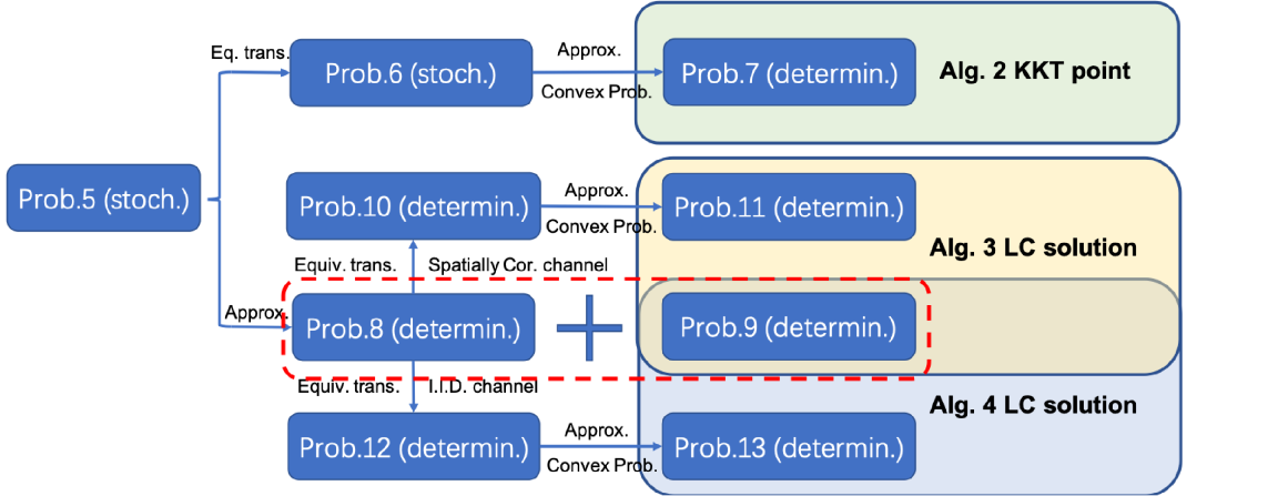
IV Ergodic Rate Maximization In Fast Fading Scenario
This section considers the fast fading scenario and maximizes the weighted sum ergodic rate under the total transmission power constraint and achievable ergodic rate constraints. The proposed solution framework for the fast fading scenario is illustrated in Fig. 4. It is noteworthy that in the fast fading scenario when general multicast degrades to unicast, the proposed solutions based on general rate splitting outperform the one based on 1-layer rate splitting in [17] due to the fact that our solution can exploit the full potential of rate splitting and obtain a KKT point.
IV-A Optimization Problem Formulation
We would like to optimize the transmission beamforming vectors and rates of sub-message units to maximize the weighted sum ergodic rate, , subject to the total transmission power constraint in (11) and the achievable ergodic rate constraints in (12). Therefore, we formulate the following problem.
Problem 5 (Weighted Sum Ergodic Rate Maximization)
where is given by (2).
Remark 4 (Connection with Rate Splitting for Unicast and Multicast)
When general multicast degrades to unicast and general rate splitting reduces to 1-layer rate splitting, Problem 5 can reduce to the weighted sum ergodic rate maximization problem for unicast in [17]. Besides, Problem 5 can be regards as a generalization the weighted sum ergodic rate maximization problem for other service types.
Note that the objective function is linear, the constraint in (11) is convex, and the constraints in (12) involve expectations and are nonconvex. Thus, Problem 5 is a more challenging nonconvex stochastic problem than the one in the slow fading scenario as it is not separable and has stochastic constraints.
IV-B KKT Point
In this subsection, we propose a stochastic iterative algorithm to obtain a KKT point of Problem 5 using SSCA together with the exact penalty method[31]. First, we equivalently transform Problem 5 to a stochastic optimization problem whose objective function is the weighted sum of the original objective function and the penalty for violating the nonconvex constraints with expectations in (12).
Problem 6 (Equivalent Problem of Problem 5)
| (21) |
where are slack variables, and is a penalty parameter that trades off the original objective function and the slack penalty term.
Next, at iteration , we choose:
with as a convex surrogate function of in (21), where is the realization of the random system channel state at iteration , is a stepsize satisfying , and
| (22) |
is a convex approximation of around . In (22), can be any constant, and the term is used to ensure strong convexity. Then, the approximation convex problem at iteration is given as follows.
Problem 7 (Approximation of Problem 5 at -th Iteration)
| (23) |
Let denote an optimal solution of Problem 7.
It is noted that Problem 7 is a convex optimization problem which is always feasible (as can be arbitrarily large). We can obtain an optimal solution of Problem 7, , with the convex optimization techniques [28]. Given , we then update according to:
| (24) |
where is a step size satisfying:
The detailed procedure is summarized in Algorithm 2. Note that Problem 7 has variables and constraints. Thus, when an interior point method is applied, the computational complexity for solving Problem 7 is as [28]. Note that the number of iterations of Algorithm 2, , is fixed, the computational complexity for Algorithm 2 is the same as that for solving Problem 7, i.e., as . As discussed in Section III-B, we can apply rate splitting with a reduced number of layers together with successive decoding to reduce the computational complexity to as in[20].
Theorem 2 (Convergence of Algorithm 2)
Proof 3
We can run Algorithm 2 multiple times, each with a random initial point and a sufficiently large , until a KKT point of Problem 6 with , i.e., a KKT point of Problem 5, is obtained.
IV-C Low-Complexity Solutions
It is noteworthy that a stochastic iterative algorithm usually converges slowly and has low computation efficiency compared with its deterministic counterpart. Thus, in this subsection, we propose two low-complexity iterative algorithms to obtain feasible points of Problem 5 with promising performance for two cases of channel distributions using approximation and CCCP. By approximating in (12) with[30]:
where represents the channel covariance matrix for user and subcarrier , we approximate the stochastic nonconvex problem in Problem 5 with the following deterministic nonconvex problem.
Problem 8 (Approximate Problem of Problem 5 for Obtaining )
| (25) |
Let denote the beamforming vectors corresponding to a KKT point of Problem 8 (which may not be feasible for Problem 5 because of the adopted approximation). Then, construct the following deterministic linear programming parametrized by .
Problem 9 (Approximate Problem of Problem 5 for Obtaining )
| (26) |
Let denote an optimal solution of Problem 9.
Proof 4
As the approximation error is usually small, can be viewed as an approximate solution of Problem 5. Based on the numerical calculation of , we can easily solve Problem 9 using standard optimization methods. Problem 9 has variables and constraints. Thus, the computational complexity for solving Problem 9 using an interior point method is . Moreover, it is expected that the deterministic nonconvex problem in Problem 8 can be more effectively solved than the stochastic nonconvex problem in Problem 5. In what follows, we concentrate on solving Problem 8 in two cases of channel distributions, namely spatially correlated channel ( has non-zero non-diagonal elements, for all ) and independent and identically distributed (i.i.d.) channel ( is a diagonal matrix with identical diagonal elements, for all ).
IV-C1 Spatially correlated channel
In this part, we consider the case of spatially correlated channel, i.e., has non-zero non-diagonal elements, for all First, using the same method as in Section III, Problem 8 can be transformed into the following DC programming by introducing auxiliary variables and extra constraints.
Problem 10 (Equivalent DC Problem of Problem 8)
| (27) | |||
| (28) | |||
| (29) |
where and (with a slight abuse of notation). Let denote an optimal solution of Problem 10.
Proof 5
The proof is similar to the one for Lemma 1 and is omitted here.
Note that and are auxiliary variables, and (27), (28), and (29) are extra constraints. Analogously, the approximation convex problem of Problem 10 at iteration is given below. Let denote an optimal solution of the following problem.
Problem 11 (Approximation of Problem 10 at Iteration )
| (30) |
where , , and
| (31) |
Similarly, Problem 11 is a convex problem and can be solved using standard convex optimization methods. Problem 11 has variables and constraints. Thus, when an interior point method is applied, the computational complexity for solving Problem 11 is as [28]. The details for obtaining a feasible point of Problem 5 are summarized in Algorithm 3. Similarly, as the number of iterations of Algorithm 1 does not scale with the problem size[29], we can conclude that the computational complexity of Steps 2-5 in Algorithm 3 is as . Recall that the computational complexity for solving Problem 9 is . Thus, the computational complexity of Algorithm 3 is as . Similarly, we can reduce the computational complexity to as in[20]. Analogously, we have the following convergence result.
Theorem 3 (Convergence of Algorithm 3)
Proof 6
The constraints in (11), (27), (28) are convex, and the constraint function in (29) can be regarded as a difference between two convex functions, i.e., and . Therefore, Problem 10 is a DC programming. Similarly, linearizing at and preserving give in (31). Thus, Steps 1-5 of Algorithm 3 implements CCCP. It has been validated in [27] that solving DC programming through CCCP always returns a KKT point. Therefore, we can show Theorem 3.
IV-C2 I.I.D. channel
In this part, we consider i.i.d. channel, i.e., is a diagonal matrix with identical diagonal elements, for all . By changing variables, i.e., letting , Problem 8 can be equivalently converted into the following problem.
Problem 12 (Equivalent problem of Problem 8 for i.i.d. channel)
| (32) | ||||
| (33) |
where . Let denote an optimal solution of Problem 12.
Note that Problem 12 for i.i.d. channel is irrelevant to , as we intend to optimize the time-invariant beamforming vectors according to channel statistics in the fast fading scenario. Problem 10 has complex optimization variables for beamforming (i.e., ) whereas Problem 12 has real optimization variables for beamforming (i.e., ). Thus, it is expected that Problem 12 has lower computational complexity than Problem 10. Besides, we have the following result.
Lemma 4 (Equivalence Between Problem 8 and Problem 12)
Any with is an optimal solution of Problem 8.
Proof 7
When , we can transform to
Problem 12 is a DC programming, and we can obtain a KKT point using CCCP. Specifically, the approximation convex problem at iteration is given below.
Problem 13 (Approximation of Problem 12 at Iteration )
| (34) |
Let denote an optimal solution of Problem 13, where .
Problem 13 is a convex problem and can be solved using standard convex optimization methods. Note that Problem 13 has variables and constraints. Thus, when an interior point method is applied, the computational complexity for solving Problem 13 is as [28]. The details for obtaining a feasible point of Problem 5 are summarized in Algorithm 4. Similarly, the computational complexity of Steps 2-5 in Algorithm 4 is as . Noting that the computational complexity for solving Problem 9 is , the computational complexity of Algorithm 4 is as . Similarly, we can reduce the computational complexity to as in[20]. Analogously, we have the following convergence result.
Theorem 4 (Convergence of Algorithm 4)
Proof 8
The constraint in (32) is linear and each constraint function of (33), can be regarded as a difference between two convex functions, and . Thus, Problem 12 is a DC programming. Linearizing at and preserving give the constraints in (34). Thus, Step 1-5 of Algorithm 4 implements CCCP. It has been validated in [27] that solving DC programming through CCCP always returns a KKT point. Therefore, we can show Theorem 4.
V Comparisons Between Slow Fading Scenario and Fast Fading Scenario
First, we compare the computational complexities for the weighted sum average rate maximization in the slow fading scenario and the weighted sum ergodic rate maximization in the fast fading scenario. Algorithm 1 (for obtaining a KKT point in the slow fading scenario based on CCCP) has higher computational complexity than Algorithm 2 (for obtaining a KKT point in the fast fading scenario based on SSCA). However, noting that SSCA converges more slowly than CCCP in general, Algorithm 2 has longer computational time to achieve satisfactory performance than Algorithm 1. Besides, Algorithm 3 (for obtaining a low complexity solution in the fast fading scenario with spatially correlated channel based on CCCP) has the same computational complexity as Algorithm 1. Last, Algorithm 4 (for obtaining a low complexity solution in the fast fading scenario with i.i.d. channel based on CCCP) has lower computational complexity than Algorithm 1.
Next, we compare the practical implementation complexities for the solutions in slow fading scenario and the fast fading scenario. In the slow fading scenario, the BS must obtain the instantaneous channel condition and adjust the beamforming vectors at each slot according to the instantaneous system channel state. By contrast, in the fast fading scenario, the BS requires only the knowledge of channel statistics and adopts constant beamforming vectors, relying on channel statistics over slots. Therefore, the practical implementation complexities in the slow fading scenario are obviously higher than the those in the fast fading scenario.
Finally, we compare the optimal values of the weighted sum average rate maximization in the slow fading scenario and weighted sum ergodic rate maximization in the fast fading scenario. As the beamforming vectors in the slow fading scenario are adjusted at each slot according to the instantaneous system channel state, it is expected that the optimal value in the slow fading scenario is larger than that in the fast fading scenario. Although the gain in the optimal value cannot be shown analytical, it will be numerically verified in Section VI.
VI Numerical Results
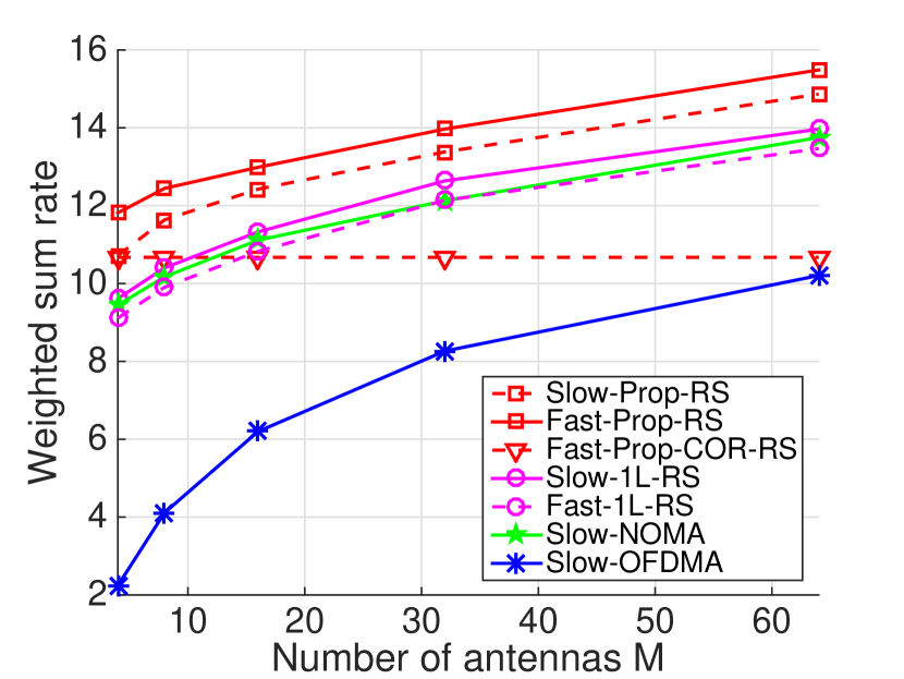
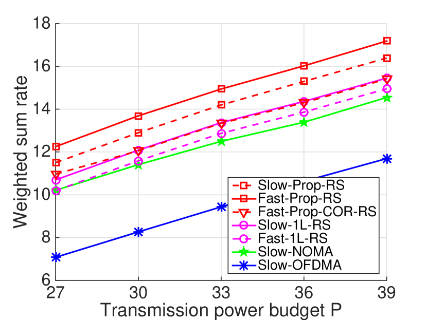
In this section, we numerically evaluate the proposed solutions obtained by Algorithm 1 for the slow fading scenario, namely Slow-Prop-RS and Algorithm 2, Algorithm 3, and Algorithm 4 for the fast fading scenario, namely Fast-Prop-RS, Fast-Prop-COR-RS, and Fast-Prop-IID-RS, respectively. In the slow fading scenario, we consider three baseline schemes, namely Slow-1L-RS, Slow-NOMA, and Slow-OFDMA. Slow-1L-RS and Slow-NOMA (both with joint decoding for fair comparison) extend 1-layer rate splitting (where each message is split into one private part and only one common part) [15] and NOMA[33], both for unicast in one slot, to general multicast in the considered slow fading scenario. More specifically, Slow-1L-RS and Slow-NOMA implement Algorithm 1 to obtain KKT points of Problem 2 with and with , respectively.121212Slow-NOMA adopts NOMA with joint decoding, which outperforms the commonly adopted NOMA with successive decoding[33]. Note that it is challenging to optimize the subsequent decoding order for NOMA in general multicast. Slow-OFDMA adopts OFDMA and considers the maximum ratio transmission (MRT) on each subcarrier and optimizes the subcarrier and power allocation[4]. In the fast fading scenario, we consider one baseline scheme, namely Fast-1L-RS.131313As existing works on NOMA and OFDMA mainly concentrate on one single slot, we do not consider their extensions to the fast fading scenario, whose performance can be far from satisfactory. Similarly, Fast-1L-RS (with joint decoding) extends 1-layer rate splitting for unicast in the fast fading scenario[17] to general multicast in the fast fading scenario. In particular, Fast-1L-RS implements Algorithm 2 to obtain a KKT point of Problem 5 with . Note that for the proposed solutions, . All algorithms adopt the same stopping criterion that the change in the objective function between two consecutive iterations is smaller than 0.1. In the slow fading scenario, we generate 100 random realizations of , solve the weighted sum rate maximization problem for each realization, and evaluate the weighted sum average rate of each scheme over the 100 random realizations. In the sequel, the weighted sum average rate in the slow fading scenario and the weighted sum ergodic rate in the fast fading scenario are both termed the weighted sum rate for ease of presentation.
In the simulation, we set , , , , and . As a result, we have , , , , , , and . Additionally, we set , = 30 kHz, = 72, and W. We consider two cases of channel distributions, i.e., spatially correlated channel with the correlation following the one-ring scattering model as in [20] and i.i.d. channel with . Note that the channel covariance matrix in the case of a spatially correlated channel is normalized for a fair comparison. When applying the one-ring scattering model, let denote the number of user groups. We set the same angular spreads for the groups and the same azimuth angle for the users in each group as in[20]. Note that is related to the channel correlation among users. Specifically, the correlation increases as decreases. When , users belong to one group and have the same channel covariance matrix. When , users are in different groups and have different channel covariance matrices.
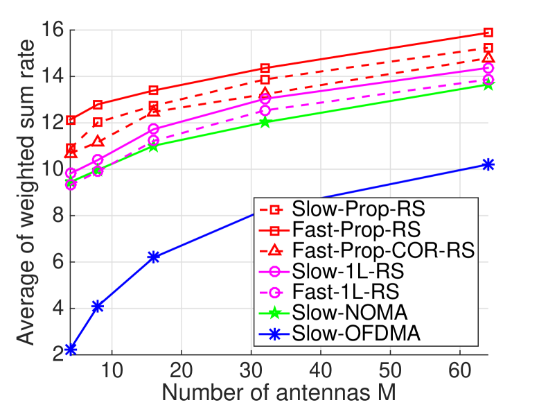
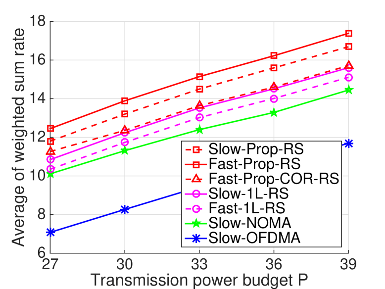
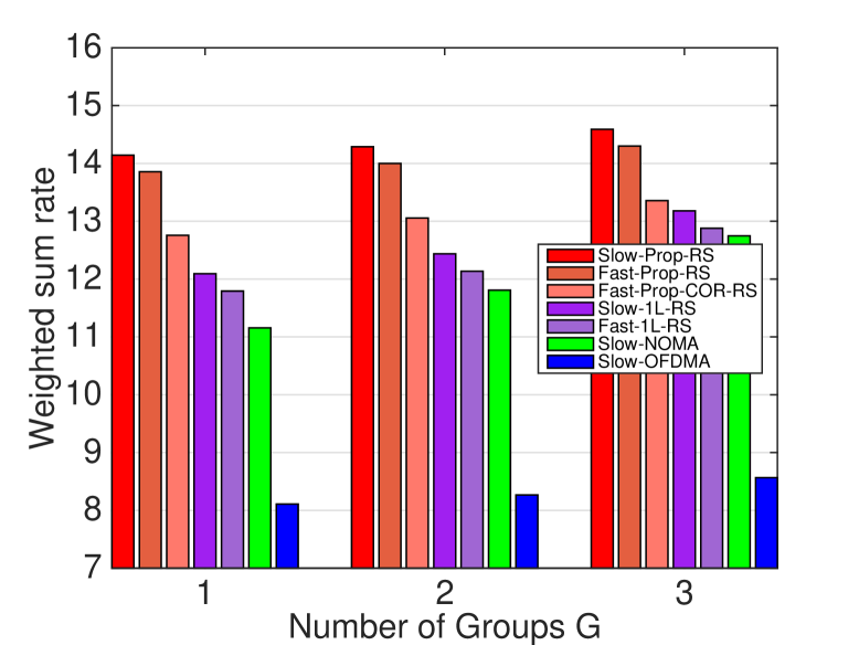
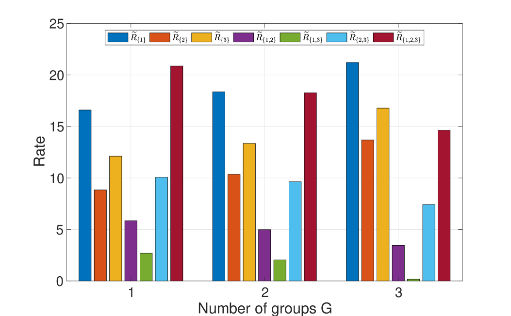
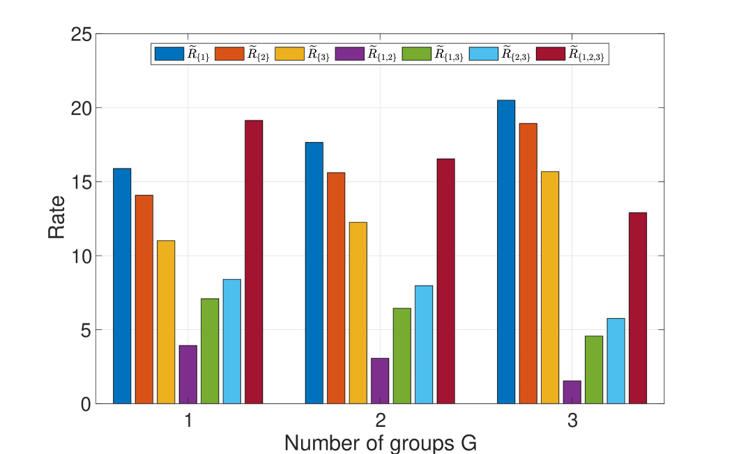
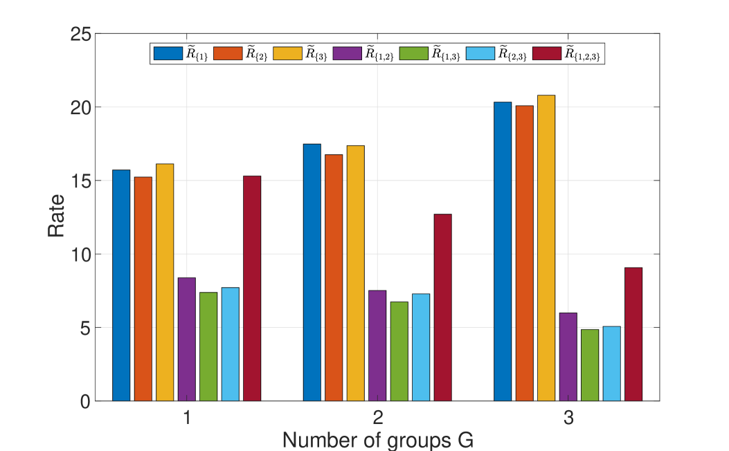
First, we show the weighted sum rate of each scheme in the case of the spatially correlated channel. Fig. 5 illustrates the weighted sum rate versus the number of transmit antennas , the total transmission power budget , and the number of user groups in the one-ring scattering model, respectively, in the case of the spatially correlated channel. From Fig. 5, we have the following observations. Firstly, the weighted sum rate of each scheme increases with , , and . Secondly, in the slow fading and fast fading scenarios, the proposed solutions outperform the corresponding baseline schemes. The gain of Slow-Prop-RS (Fast-Prop-RS or Fast-Prop-COR-RS) over Slow-1L-RS (Fast-1L-RS) is because each proposed solution unleashes the full potential of the flexibility of rate splitting. The gain of Slow-Prop-RS over Slow-NOMA arises because the cost for Slow-NOMA to suppress interference is high. In contrast, rate splitting together with joint decoding partially decodes interference and partially treats interference as noise. The gain of Slow-Prop-RS over Slow-OFDMA comes from an effective nonorthogonal transmission design. Thirdly, Slow-Prop-RS (Slow-1L-RS) outperforms Fast-Prop-RS (Fast-1L-RS). The gain arises from the fact that Slow-Prop-RS (Slow-1L-RS) optimizes the beamforming vectors at each slot according to the instantaneous system channel state, whereas Fast-Prop-RS (Fast-1L-RS) adopts the time-invariant beamforming vectors which are optimized according to the channel statistics. Additionally, Fig. 5 (c) shows that the gain of Slow-Prop-RS (Fast-Prop-RS or Fast-Prop-COR-RS) over Slow-1L-RS (Fast-1L-RS) and the gain of Slow-Prop-RS over Slow-NOMA increase as decreases, demonstrating the advantage of flexibly dealing with interference in the presence of channel correlation among users. Fig. 6 shows the rates of the transmission units in each proposed solution versus the number of user groups in the case of the spatially correlated channel. We can see that for each proposed solution, and increase with , whereas and decrease with . This is because as channel correlation among the users decreases, it is efficient to decode less interference and treat more interference as noise.
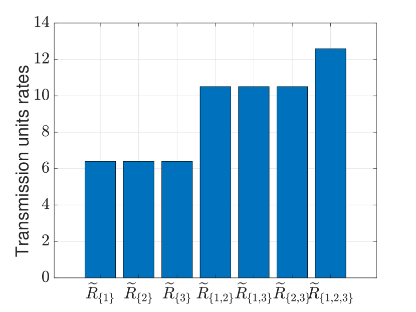
Next, we show the weighted sum rate of each scheme in the case of the i.i.d. channel. Fig. 9 and Fig. 9 plot the weighted sum rate versus the number of transmit antennas and the total transmission power budget in the case of the i.i.d. channel. We observe from these two figures that the weighted sum rate of Fast-Prop-IID-RS does not change with . This is because Problem 12 is irrelevant to . Besides, we have the same observations as from Fig. 5 (a) and (b). Fig. 9 shows the rates of the transmission units of Fast-Prop-IID-RS in the case of the i.i.d. channel. We can see from Fig. 9 that , and are identical, and , and are identical. The reasons are as follows. The general multicast setup is symmetric w.r.t. all users and their requesting messages, i.i.d. channel is considered, and time-invariant beamforming is adopted in the fast fading scenario.
VII Conclusion
While applications such as content delivery are responsible for a large and increasing fraction of Internet traffic, general multicast communication will play a central role for future 6G and beyond networks. This paper investigated the optimization of general rate splitting for general multicast. We optimized the transmission beamforming vectors and rates of sub-message units to maximize the weighted sum average rate and the weighted sum ergodic rate in the slow fading and fast fading scenarios, respectively. We proposed iterative algorithms to obtain KKT points and low-complexity solutions in both scenarios using various optimization techniques. The proposed optimization framework generalizes the existing ones for rate splitting for unicast, unicast with a common message, single-group multicast, and multi-group multicast. Numerical results demonstrate notable gains of the proposed solutions over existing schemes and reveal the impact of channel correlation among users on the performance of general rate splitting for general multicast.
There are still some key aspects that we leave for future investigations. One direction is to go beyond linear approaches and investigate nonlinear precoders such as binning[34, 9]. Another interesting perspective is general multicast with partial channel state information at the transmitter side[35, 20].
References
- [1] “Virtual reality (VR) market - growth, trends, and forecast (2020 - 2025),” Mordor Intelligence, Jan. 2020. [Online]. Available: https://www.mordorintelligence.com/industry-reports/virtualreality-market/
- [2] K. Long, Y. Cui, C. Ye, and Z. Liu “Optimal wireless streaming of multi-quality 360 VR video by exploiting natural, relative smoothness-enabled and transcoding-enabled multicast opportunities,” IEEE Trans. Multimedia, vol. 23, pp. 3670-3683, Oct. 2021.
- [3] W. Xu, Y. Cui, and Z. Liu, “Optimal multi-view video transmission in multiuser wireless networks by exploiting natural and view synthesisenabled multicast opportunities,” IEEE Trans. Commun., vol. 68, no. 3, pp. 1494-1507, Mar. 2020.
- [4] C. Guo, L. Zhao, Y. Cui, Z. Liu, and D. Ng ”Power-efficient transmission of multi-quality tiled 360 VR video in MIMO-OFDMA systems,” IEEE Trans. Wireless Commun., vol. 20, no. 8, pp. 5408-5422, Aug. 2021.
- [5] W. Xu, Y. Cui, Z. Liu, and H. Li, “Optimal multi-view video transmission in OFDMA systems,” IEEE Commun. Lett., vol. 24, no. 3, pp. 667-671, Mar. 2020.
- [6] Y. Mao, O. Dizdar, B. Clerckx, R. Schober, P. Popovski, and H. V. Poor, “Rate-splitting multiple access: fundamentals, survey, and future research trends,” arXiv preprint arXiv:2201.03192, Jan. 2022.
- [7] Y. Cui, M. Médard, E. Yeh, D. Leith, F. Lai, and K. R. Duffy, ”A linear network code construction for general integer connections based on the constraint satisfaction problem,” IEEE/ACM Trans. Netw., vol. 25, no. 6, pp. 3441-3454, Dec. 2017.
- [8] Y. Cui, M. Médard, E. Yeh, D. Leith, and K. R. Duffy, “Optimization-based linear network coding for general connections of continuous flows,” IEEE/ACM Trans. Netw., vol. 26, no. 5, pp. 2033-2047, Oct. 2018.
- [9] H. P. Romero and M. K. Varanasi, ”Rate splitting, superposition coding and binning for groupcasting over the broadcast channel: A general framework,” arXiv preprint arXiv:2011.04745, Nov. 2020.
- [10] T. Yoo and A. Goldsmith, “On the optimality of multiantenna broadcast scheduling using zero-forcing beamforming,” IEEE J. Sel. Areas Commun., vol. 24, no. 3, pp. 528–541, Mar. 2006.
- [11] Z. Li, S. Yang, and S. Shamai, “On linearly precoded rate splitting for gaussian MIMO broadcast channels,” IEEE Trans. Inf. Theory, vol. 67, no. 7, pp. 4693-4709, Jul. 2021.
- [12] T. Han and K. Kobayashi, “A new achievable rate region for the interference channel,” IEEE Trans. Inf. Theory, vol. 27, no. 1, pp. 49-60, Jan. 1981.
- [13] S. Yang, M. Kobayashi, D. Gesbert, and X. Yi, “Degrees of freedom of time correlated MISO broadcast channel with delayed CSIT,” IEEE Trans. Inf. Theory, vol. 59, no. 1, pp. 315-328, Jan. 2013.
- [14] J. Park, J. Choi, N. Lee, W. Shin, and H. V. Poor, “Rate-splitting multiple access for downlink MIMO: A generalized power iteration approach,” arXiv preprint arXiv:2108.06844, Aug. 2021.
- [15] H. Joudeh and B. Clerckx, “Robust transmission in downlink multiuser MISO systems: A rate-splitting approach,” IEEE Trans. Signal Process., vol. 64, no. 23, pp. 6227–6242, Dec. 2016.
- [16] Y. Mao, B. Clerckx, J. Zhang, V. O. K. Li, and M. A. Arafah, “Max-min fairness of K-user cooperative rate-splitting in MISO broadcast channel with user relaying,” IEEE Trans. Wireless Commun., vol. 19, no. 10, pp. 6362-6376, Oct. 2020.
- [17] H. Joudeh and B. Clerckx, “Sum-rate maximization for linearly precoded downlink multiuser MISO systems with partial CSIT: A rate-splitting approach,” IEEE Trans. Commun., vol. 64, no. 11, pp. 4847–4861, Nov. 2016.
- [18] Z. Yang, M. Chen, W. Saad, and M. Shikh-Bahaei, “Optimization of rate allocation and power control for rate splitting multiple access (RSMA),” IEEE Trans. Commun., vol. 69, no. 9, pp. 5988-6002, Sep. 2021.
- [19] Y. Mao, B. Clerckx, and V. O. K. Li, “Rate-splitting multiple access for downlink communication systems: Bridging, generalizing, and outperforming SDMA and NOMA,” EURASIP JWCN, vol. 2018, no. 1, p. 133, May 2018.
- [20] Z. Li, C. Ye, Y. Cui, S. Yang, and S. Shamai, “Rate splitting for multi-antenna downlink: Precoder design and practical implementation,” IEEE J. Select. Areas Commun., vol. 38, no. 8, pp. 1910–1924, Jun. 2020.
- [21] Y. Mao, B. Clerckx, and V. O.K. Li, “Rate-splitting for multi-antenna non-orthogonal unicast and multicast transmission: spectral and energy efficiency analysis,” IEEE Trans. Commun., vol. 67, no. 12, pp. 8754-8770, Dec. 2019.
- [22] L. Yin, B. Clerckx, and Y. Mao, ”Rate-splitting multiple access for multi-antenna broadcast channels with statistical CSIT,” in Proc. of IEEE WCNCW, Mar. 2021, pp. 1-6.
- [23] H. Joudeh and B. Clerckx, “Rate-splitting for max-min fair multigroup multicast beamforming in overloaded systems,” IEEE Trans. Wireless Commun., vol. 16, no. 11, pp. 7276-7289, Nov. 2017.
- [24] A. Z. Yalcin, M. Yuksel, and B. Clerckx, “Rate splitting for multi-group multicasting with a common message,” IEEE Trans. Veh. Technol., vol. 69, no. 10, pp. 12281-12285, Oct. 2020.
- [25] H. Chen, D. Mi, B. Clerckx, Z. Chu, J. Shi, and P. Xiao, “Joint power and subcarrier allocation optimization for multigroup multicast systems with rate splitting,” IEEE Trans on Veh. Technol., vol. 69, no. 2, pp. 2306-2310, Feb. 2020.
- [26] N. D. Sidiropoulos, T. N. Davidson and Z. Luo, “Transmit beamforming for physical-layer multicasting,” IEEE Trans. Signal Process., vol. 54, no. 6, pp. 2239-2251, Jun. 2006.
- [27] Y. Sun, P. Babu, and D. P. Palomar, “Majorization-minimization algorithms in signal processing, communications, and machine learning,” IEEE Trans. Signal Process., vol. 65, no. 3, pp. 794–816, Feb. 2017.
- [28] S. Boyd and L. Vandenberghe, Convex optimization. Cambridge university press, 2004.
- [29] F. Facchinei, V. Kungurtsev, L. Lampariello, and G. Scutari, “Ghost penalties in nonconvex constrained optimization: Diminishing stepsizes and iteration complexity,” Math. Oper. Res., vol. 46, no. 2, pp. 595-627, Feb. 2021.
- [30] Cover, Thomas M. Elements of information theory. John Wiley & Sons, 1999.
- [31] C. Ye and Y. Cui, “Stochastic successive convex approximation for general stochastic optimization problems,” IEEE Wireless Commun. Lett., vol. 9, no. 6, pp. 755-759, Jun. 2020.
- [32] A. Adhikary, J. Nam, J. Y. Ahn, and G. Caire, “Joint spatial division and multiplexing—The large-scale array regime,” IEEE Trans. Inf. Theory, vol. 59, no. 10, pp. 6441–6463, Oct. 2013.
- [33] L. Dai, B. Wang, Y. Yuan, S. Han, I. Chih-lin, and Z. Wang, “Non-orthogonal multiple access for 5G: solutions, challenges, opportunities, and future research trends,” IEEE Commun. Mag., vol. 53, no. 9, pp. 74-81, Sep. 2015.
- [34] R. Tang, S. Xie, and Y. Wu, “On the achievable rate region of the -receiver broadcast channels via exhaustive message splitting,” Entropy, vol. 23, no. 11: 1408, Oct. 2021.
- [35] Y. Mao and B. Clerckx, “Beyond dirty paper coding for multi-antenna broadcast channel with partial CSIT: A rate-splitting approach,” IEEE Trans. Commun., vol. 68, no. 11, pp. 6775-6791, Nov. 2020.
- [36] A. A. Ahmad, Y. Mao, A. Sezgin, and B. Clerckx, “Rate splitting multiple access in C-RAN: A scalable and robust design,” IEEE Trans. Commun., vol. 69, no. 9, pp. 5727-5743, Sep. 2021.