Bose-Einstein Condensation, the Lambda Transition, and Superfluidity for Interacting Bosons

Abstract

Bose-Einstein condensation and the $\lambda$-transition are described in molecular detail for bosons interacting with a pair potential. New phenomena are identified that are absent in the usual ideal gas treatment. Monte Carlo simulations of Lennard-Jones helium-4 neglecting ground momentum state bosons give a diverging heat capacity approaching the transition. Pure permutation loops give continuous growth in the occupancy of the ground momentum state. Mixed ground and excited momentum state permutation loops give a discontinuous transition to the condensed phase. The consequent latent heat for the $\lambda$-transition is 3% of the total energy. The predicted critical velocity for superfluid flow is within a factor of three of the measured values over three orders of magnitude in pore diameter.

I Introduction

The spike in the heat capacity and the onset of superfluidity in liquid helium-4 at 2.17 K is known as the $\lambda$-transition. London (1938) suggested that it was due to Bose-Einstein condensation, based upon analysis of the ideal gas that also showed a peak in the heat capacity as the ground energy state first begins to fill at 3.1 K. Using this ideal gas model Tisza (1938) developed a two-fluid model for superfluidity in which the ground energy state bosons were said to flow without viscosity, transparent to the excited energy state bosons that were said to have the ordinary viscosity. Landau (1941) modified Tisza’s (1938) model to include collective behavior for interacting bosons as quantum excitations (phonons). He postulated the existence of rotons, whose energy spectrum he fitted to measured heat capacity data. Later theoretical work focussed on interpreting rotons as quantized vortices (Feynman 1954, Kawatra and Pathria 1966, Pathria 1972), although direct evidence for this is lacking. Accounts of the fascinating history of the $\lambda$-transition and superfluidity have been given by Donnelly (1995, 2009) and by Balibar (2014, 2017).

The main limitation of London’s (1938) and Tisza’s (1938) approaches is that they use the ideal gas, which neglects the interactions between the helium atoms, which very interactions are responsible for the liquid state. Landau’s (1941) attempt to include interactions via phonons and rotons may be criticized as lacking a specific molecular basis, and as being disconnected from any phase transition, including Bose-Einstein condensation. In addition all three approaches lack a derivation of superfluidity that explains the absence of viscosity in the presence of molecular interactions (i.e. collisions).

The present paper analyzes the $\lambda$-transition for interacting bosons. Section II gives a re-analysis of London’s (1938) ideal gas approach with the focus on a particular approximation that separates the ground energy state from the continuum integral for the excited states. Here and in the rest of the paper the analysis invokes momentum states and permutation loops for wave function symmetrization. These are the basis of the author’s formulation of quantum statistical mechanics in classical phase space (Attard 2018, 2021). The reader may be assured that for the ideal gas these give the same results as obtained originally by London (1938).

Section III generalizes the ideal gas treatment, including the separation of the ground momentum state from the excited momentum continuum, to bosons interacting with arbitrary pair and many-body potentials. Monte Carlo simulation results show the dependence upon the interaction potential of the heat capacity and the $\lambda$-transition temperature. A mean field theory based on pure permutation loops is developed and results are given for ground momentum state occupancy using input from Monte Carlo simulations of Lennard-Jones helium-4. The resultant heat capacity in the vicinity of the $\lambda$-transition is shown in Fig. 1 and is discussed in section IV.4 below.

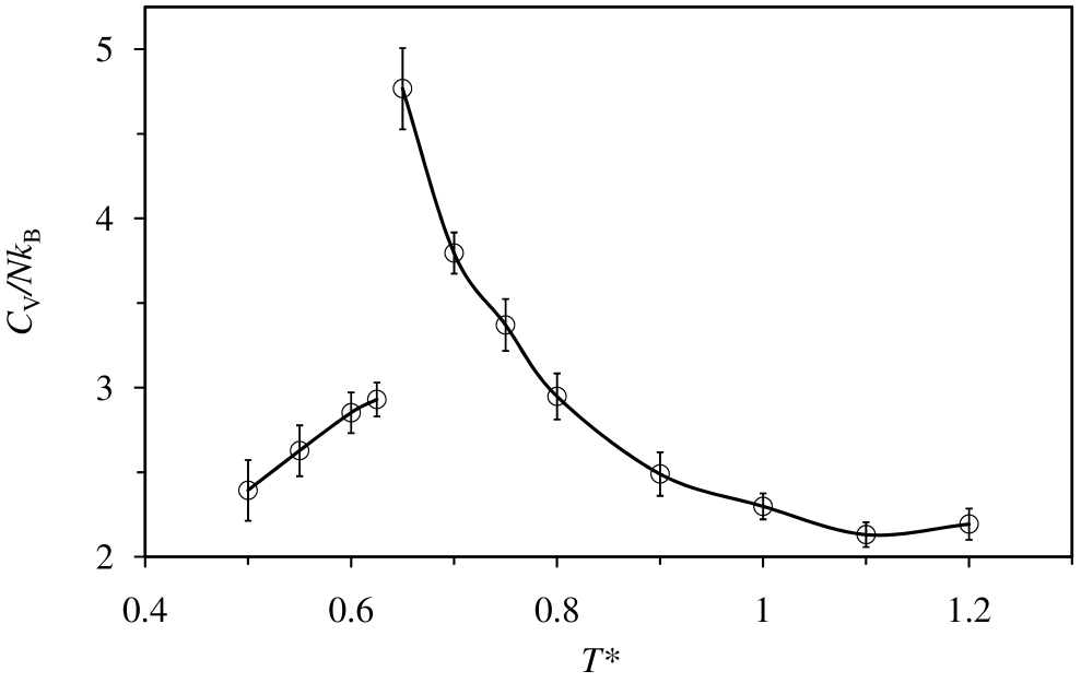
Figure 1: The $\lambda$-transition in a Lennard-Jones fluid. The specific heat is obtained by Monte Carlo simulation using pentamer permutation loops. Below the condensation temperature the ground momentum state occupancy is obtained from the pure permutation loop approximation, § III.2. Note that for ⁴He, $T[K]=10.22T^{*}$.

Section IV analyzes mixed permutation loops. Monte Carlo dimer results show that the occupancy of the ground momentum state occurs discontinuously at the $\lambda$-transition, which is confirmed by results for higher order mixed loops. The discontinuity implies a latent heat. In section IV.3 dressed ground momentum state bosons are formulated in a type of ideal solution theory that locates the condensation transition in Fig. 1.

The present paper extends the analysis of the $\lambda$-transition and Bose-Einstein condensation given in chapter 5 of Attard (2021). That chapter gives the computational details and a molecular-level discussion of the physical nature of the $\lambda$-transition and superfluidity.

II Ideal Gas

In general the grand potential of a quantum system may be expressed as a series of permutation loop grand potentials Attard (2018, 2021),

$$\Omega(z,V,T)=\sum_{l=1}^{\infty}\Omega^{(l)}(z,V,T).$$ (2.1)

Here $z=e^{\beta\mu}$ is the fugacity, $V=L^{3}$ is the volume, and $T=1/k_{\mathrm{B}}\beta$ is the temperature. The monomer $l=1$ contribution to this is the classical contribution.

The ideal gas loop grand potential is exactly

$$-\beta\Omega^{(l)} = \frac{z^{l}}{l}\sum_{n_{x},n_{y},n_{z}}e^{-l\beta n^{2}\Delta_{p}^{2}/2m},\;\;l\geq 1.$$ (2.2)

Here the spacing of momentum states is $\Delta_{p}=2\pi\hbar/L$ (Messiah 1961, Merzbacher 1970). The boson mass is $m$, and $\hbar$ is Planck’s constant divided by $2\pi$.

Now transform the sum over states to a continuum integral. In order to analyze the approximation introduced by London (1938), we need to retain the discrete ground momentum state explicitly. Therefore to correct for double counting, we need to subtract the integral over the ground momentum state interval. This gives

$$-\beta\Omega^{(l)} = \frac{z^{l}}{l}\left[1+\Delta_{p}^{-3}\int\mathrm{d}{\bf p}\;e^{-l\beta p^{2}/2m}\right.$$ (2.3)

$$\mbox{ }\left.-\Delta_{p}^{-3}\int_{\Delta_{p}^{3}}\mathrm{d}{\bf p}\;e^{-l\beta p^{2}/2m}\right]$$

$$= \frac{z^{l}}{l}\left[1+\left(\frac{L^{2}}{l\Lambda^{2}}\right)^{3/2}\right.$$

$$\mbox{ }\left.-\left(\frac{L^{2}}{l\Lambda^{2}}\right)^{3/2}\;\mbox{erf}\!\left(\sqrt{\frac{2\pi l\Lambda^{2}}{8L^{2}}}\right)^{3}\right].$$

The thermal wave length is $\Lambda=\sqrt{2\pi\hbar^{2}\beta/m}$.

The asymptotic forms of the error function are $\mbox{erf}(x)\sim({2}/{\surd\pi})x$, $x\rightarrow 0$, and $\mbox{erf}(x)\sim 1-{e^{-x^{2}}}/{\sqrt{\pi}\,x}$, $x\rightarrow\infty$ (Abramowitz and Stegun 1970). It follows that the limiting results for the loop grand potential are

$$-\beta\Omega^{(l)} \sim \left\{\begin{array}[]{ll}\displaystyle\frac{z^{l}}{l}\left(\frac{L^{2}}{l\Lambda^{2}}\right)^{3/2},&l\Lambda^{2}/L^{2}\ll 1,\\ \displaystyle\rule{0.0pt}{19.91692pt}\frac{z^{l}}{l},&l\Lambda^{2}/L^{2}\gg 1.\end{array}\right.$$ (2.6)

In the limit of small argument, $l\Lambda^{2}/L^{2}\ll 1$ (high temperature, small loops), the two ground state contributions cancel exactly and only the integral over excited states survives. In the limit of large argument, $l\Lambda^{2}/L^{2}\gg 1$ (low temperature, large loops), the integral over excited states cancels with the integral about the ground state, and only the discrete ground state contribution survives.

Each of these two asymptotic limits dominates the other in its respective regime. Hence if we simply add them together the resultant function is guaranteed correct in both asymptotic limits,

$$-\beta\Omega^{(l)} \approx \frac{z^{l}}{l}+\frac{z^{l}}{l}\left(\frac{L^{2}}{l\Lambda^{2}}\right)^{3/2}$$ (2.7)

$$\equiv -\beta\Omega^{(l)}_{0}-\beta\Omega^{(l)}_{*}.$$

When summed over $l$ this gives

$$-\beta\Omega = -\ln[1-z]+\Lambda^{-3}V\sum_{l=1}^{\infty}z^{l}l^{-3/2}$$ (2.8)

$$\equiv -\beta\Omega_{0}-\beta\Omega_{*}.$$

This is the expression given by London (1938) (see also Pathria (1972 chapter 7)). The first term is the discrete ground state contribution and the second term is the continuum excited state contribution. The contribution from the ground state correction integral about the origin has been neglected. One sees that the approximate expression gives the correct result in the two respective asymptotic limits. It might therefore be expected to be a reasonable approximation throughout.

The conventional derivation (c.f. Pathria 1972 chapter 7) asserts that the discrete ground energy state must be added explicitly to the continuum over the excited energy states because the volume element for energy, $\mathrm{d}\varepsilon\,\varepsilon^{1/2}\propto\mathrm{d}p\,p^{2}$, vanishes at zero and therefore the integral does not include any contribution from the ground state. But this is mathematical nonsense, since the continuum integral includes contributions from the neighborhood of the origin, $|p_{x}|\leq\Delta_{p}/2$ etc., and it is double counting to include the discrete ground state in addition to the continuum integral. The real justification for London’s (1938) approximation is that it is correct in the two asymptotic limits, and therefore one can hope that it remains accurate throughout its entire domain.

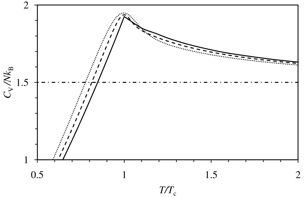
Figure 2: Specific heat of ideal bosons. The solid curve uses the London (1938) approximation, Eq. (2.7) (discrete ground state plus continuum excited states), and the remaining curves use the exact summation over all momentum states, Eq. (2.2). The density is fixed at $\rho=0.3$ with $N=500$ (dotted) or $N=5000$ (short dashed). The condensation temperature $T_{\mathrm{c}}$ was defined by the location of the maximum for each curve. The dash-dotted line is the classical result. Data from Attard (2021).

The London (1938) approximation is tested against exact benchmarks in Fig. 2 (Attard 2021 sections 5.1 and 5.2). One can see that the approximation is very good, and that it gets better with increasing system size. One might speculate that it would become exact in the thermodynamic limit.

Unfortunately one cannot so easily check the analogous formulation for interacting systems. One should bear this point in mind in judging the following results for interacting bosons. These also invoke the London (1938) approximation of simply adding the discrete ground momentum state to the continuum integral over the excited momentum states with no correction for double counting.

III Interacting Bosons

III.1 Formal Analysis

Consider a system of $N$ identical bosons interacting with potential energy $U({\bf q}^{N})$, or more simply $U({\bf q})$, which does not depend on the momentum state of the bosons. At any instant there are $N_{0}$ bosons in the ground momentum state and $N_{*}$ in excited momentum states, with $N=N_{0}+N_{*}$. The notation $j\in N_{0}$ labels a ground momentum state boson and $j\in N_{*}$ labels an excited momentum state boson. The momentum eigenvalue of boson $j$ is ${\bf p}_{j}$. The classical kinetic energy is ${\cal K}({\bf p}^{N})={\cal K}({\bf p}^{N_{*}})=\sum_{j}^{N_{*}}p_{j}^{2}/2m=p^{2}/2m$. The normalized momentum eigenfunctions for the discrete momentum case are $|{\bf p}\rangle=V^{-N/2}e^{-{\bf q}\cdot{\bf p}/\mathrm{i}\hbar}$. The system has volume $V=L^{3}$ and the spacing between momentum states is $\Delta_{p}=2\pi\hbar/L$ (Messiah 1961, Merzbacher 1970).

The grand partition function for bosons is (Attard 2018, 2021)

$$\Xi = \mbox{TR}^{\prime}\;e^{-\beta\hat{\cal H}}$$ (3.1)

$$= \sum_{N=0}^{\infty}\frac{z^{N}}{N!}\sum_{\hat{\mathrm{P}}}\sum_{\bf p}\left\langle\hat{\mathrm{P}}{\bf p}\left|e^{-\beta\hat{\cal H}}\right|{\bf p}\right\rangle$$

$$= \sum_{N=0}^{\infty}\frac{z^{N}}{N!}\sum_{\hat{\mathrm{P}}}\sum_{\bf p}\int\mathrm{d}{\bf q}\;\left\langle\hat{\mathrm{P}}{\bf p}|{\bf q}\right\rangle\,\left\langle{\bf q}\left|e^{-\beta\hat{\cal H}}\right|{\bf p}\right\rangle$$

$$\approx \sum_{N=0}^{\infty}\frac{z^{N}}{N!V^{N}}\sum_{\hat{\mathrm{P}}}\sum_{\bf p}\int\mathrm{d}{\bf q}\;e^{-\beta{\cal H}({\bf q},{\bf p})}\frac{\left\langle\hat{\mathrm{P}}{\bf p}|{\bf q}\right\rangle}{\left\langle{\bf p}|{\bf q}\right\rangle}$$

$$= \sum_{N=0}^{\infty}\frac{z^{N}}{N!V^{N}}\sum_{\bf p}\int\mathrm{d}{\bf q}\;e^{-\beta{\cal H}({\bf q},{\bf p})}\eta({\bf q},{\bf p}).$$

The permutation operator is $\hat{\mathrm{P}}$. In the penultimate equality the commutation function has been neglected; the error introduced by this approximation is negligible in systems that are dominated by long range effects (Attard 2018, 2021). The classical Hamiltonian phase space function is ${\cal H}({\bf q},{\bf p})={\cal K}({\bf p})+U({\bf q})$. The symmetrization function $\eta({\bf q},{\bf p})$ is the sum of Fourier factors over all boson permutations.

We shall now invoke the London (1938) approximation, namely transform to the momentum continuum, include the ground momentum state separately, and neglect the continuum integral correction around the momentum ground state. This gives

$$\Xi = \sum_{N=0}^{\infty}\frac{z^{N}}{N!V^{N}}\prod_{n=1}^{N}\left\{\delta_{{\bf p}_{n},{\bf 0}}+\Delta_{p}^{-3}\int\mathrm{d}{\bf p}_{n}\;\right\}$$ (3.2)

$$\mbox{ }\times\int\mathrm{d}{\bf q}^{N}\;e^{-\beta{\cal H}({\bf q}^{N},{\bf p}^{N})}\eta({\bf q}^{N},{\bf p}^{N})$$

$$= \sum_{N=0}^{\infty}\frac{z^{N}}{N!V^{N}}\sum_{N_{0}=0}^{N}\frac{N!\,\Delta_{p}^{-3N_{*}}}{N_{0}!N_{*}!}\int\mathrm{d}{\bf p}^{N_{*}}\;e^{-\beta{\cal K}({\bf p}^{N_{*}})}$$

$$\mbox{ }\times\int\mathrm{d}{\bf q}^{N}\;e^{-\beta U({\bf q}^{N})}\eta({\bf q}^{N},{\bf p}^{N}).$$

In the final equality there are $N_{0}$ ground momentum state bosons and $N_{*}=N-N_{0}$ excited momentum state bosons; one could write instead $\sum_{N,N_{0}}\Rightarrow\sum_{N_{0},N_{*}}$. All $N$ bosons contribute to the potential energy and to the symmetrization function. Also ${\bf p}_{j}={\bf 0}$ if $j\in N_{0}$.

III.2 Pure Loops

The symmetrization function is the sum of all permutations of the bosons in the Fourier factors. Each permutation can be expressed as a product of disjoint permutation loops (Attard 2018, 2021). In the present context permutation loops can be classified as pure or mixed. A pure permutation loop consists only of ground momentum state bosons, or only of excited momentum state bosons. A mixed permutation loop contains both.

In this section we shall pursue the leading order approximation in which all mixed permutation loops are neglected,

$$\eta({\bf q}^{N},{\bf p}^{N})\approx\eta_{0}({\bf q}^{N_{0}},{\bf p}^{N_{0}})\eta_{*}({\bf q}^{N_{*}},{\bf p}^{N_{*}}).$$ (3.3)

Here $\eta_{0}$ is the sum total of weighted permutations of ground momentum state bosons. Since their momentum is zero, ${\bf p}_{j}={\bf 0}$, $j\in N_{0}$, one has that

$$\frac{\left\langle\hat{\mathrm{P}}{\bf p}^{N_{0}}|{\bf q}^{N_{0}}\right\rangle}{\left\langle{\bf p}^{N_{0}}|{\bf q}^{N_{0}}\right\rangle}=1,\mbox{ all }\hat{\mathrm{P}}.$$ (3.4)

Hence

$$\eta_{0}({\bf q}^{N_{0}},{\bf p}^{N_{0}})=N_{0}!.$$ (3.5)

Of relevance to the later discussion of superfluidity, this result is a manifestation of quantum non-locality for ground momentum state bosons. All the ground momentum state bosons in the system contribute equally regardless of spatial location.

The remaining factor $\eta_{*}$ is the sum total of weighted permutations of excited momentum state bosons. In previous work (Attard 2021) the number of discrete ground momentum state bosons was taken to be negligible, $N_{0}=0$ and the continuum integral over momentum space was applied to all $N$ bosons. Hence all of those previous formal results carry over directly to the present case of pure excited momentum state permutation loops with the replacement $N\Rightarrow N_{*}$. (An adjustment has to be made to the statistical averages when the ground momentum state bosons are not negligible, as is discussed below.) In particular, $\eta_{*}$, is a sum of products of loops. One can define $\stackrel{{\scriptstyle\circ}}{{\eta}}\!_{*}=\sum_{l\geq 2}\eta^{(l)}_{*}$ as the sum of single loops, and one can write either

$$\eta_{*}({\bf q}^{N_{*}},{\bf p}^{N_{*}})=\exp\stackrel{{\scriptstyle\circ}}{{\eta}}\!_{*}({\bf q}^{N_{*}},{\bf p}^{N_{*}}),$$ (3.6)

or else

$$\langle\eta_{*}\rangle_{\mathrm{cl}}=e^{\langle\stackrel{{\scriptstyle\circ}}{{\eta}}\!_{*}\rangle_{\mathrm{cl}}}.$$ (3.7)

One can drop the subscript $*$ on $\eta$ when the bosons that contribute are obvious from its arguments.

It may be helpful to illustrate these two result by writing out the first few terms of the permutation series explicitly,

$$\eta({\bf q}^{N_{*}},{\bf p}^{N_{*}})$$ (3.8)

$$= 1+\sum_{j,k}^{N_{*}}\!{}^{\prime\prime}\;e^{-{\bf p}_{j}\cdot{\bf q}_{jk}/\mathrm{i}\hbar}e^{-{\bf p}_{k}\cdot{\bf q}_{kj}/\mathrm{i}\hbar}$$

$$\mbox{ }+\sum_{j,k,n}^{N_{*}}\!{}^{\prime\prime}\;e^{-{\bf p}_{j}\cdot{\bf q}_{jk}/\mathrm{i}\hbar}e^{-{\bf p}_{k}\cdot{\bf q}_{kn}/\mathrm{i}\hbar}e^{-{\bf p}_{n}\cdot{\bf q}_{nj}/\mathrm{i}\hbar}$$

$$\mbox{ }+\sum_{j,k,n,m}^{N_{*}}{}^{\prime\prime}\hskip 5.69054pte^{-{\bf p}_{j}\cdot{\bf q}_{jk}/\mathrm{i}\hbar}e^{-{\bf p}_{k}\cdot{\bf q}_{kj}/\mathrm{i}\hbar}$$

$$\hskip 51.21504pt\times e^{-{\bf p}_{n}\cdot{\bf q}_{nm}/\mathrm{i}\hbar}e^{-{\bf p}_{m}\cdot{\bf q}_{mn}/\mathrm{i}\hbar}$$

$$\mbox{ }+\ldots$$

$$= 1+\eta^{(2)}({\bf q}^{N_{*}},{\bf p}^{N_{*}})+\eta^{(3)}({\bf q}^{N_{*}},{\bf p}^{N_{*}})$$

$$\mbox{ }+\frac{1}{2}\eta^{(2)}({\bf q}^{N_{*}},{\bf p}^{N_{*}})^{2}+\ldots$$

The double prime indicates that the sums are over unique permutations, and also that in any product term no boson may belong to more than one permutation loop. The first term is the monomer or unpermuted one, and it gives rise to classical statistics. The second term is the dimer, the third is the trimer, and the fourth is the double dimer. The second equality no longer forbids permutation loop intersections; the error from this approximation ought to be negligible in the thermodynamic limit.

In view of these results, in particular the one that writes the classical average of the full symmetrization function as the exponential of the classical average of the single loop symmetrization function, it is straightforward to write the grand potential as the sum of loop grand potentials,

$$\Omega(z,V,T) = -k_{\mathrm{B}}T\ln\Xi(z,V,T)$$ (3.9)

$$= \sum_{l=1}^{\infty}\Omega^{(l)}_{*}(z,V,T).$$

The monomer grand potential is just the classical grand potential, with a trivial adjustment for $N_{0}$ and $N_{*}$ as independent. It is given by

$$e^{-\beta\Omega^{(1)}(z,V,T)} = \Xi_{\mathrm{cl}}(z,V,T)$$ (3.10)

$$= \sum_{N_{0},N_{*}}\frac{z^{N}\Delta_{p}^{-3N_{*}}}{N_{*}!V^{N}}\int\mathrm{d}{\bf p}^{N_{*}}\;e^{-\beta{\cal K}({\bf p}^{N_{*}})}$$

$$\mbox{ }\times\int\mathrm{d}{\bf q}^{N}\;e^{-\beta U({\bf q}^{N})}$$

$$= \sum_{N_{0},N_{*}}\frac{z^{N}\Lambda^{-3N_{*}}}{N_{*}!V^{N_{0}}}\int\mathrm{d}{\bf q}^{N}\;e^{-\beta U({\bf q}^{N})}$$

$$= \sum_{N_{0},N_{*}}\frac{z^{N}\Lambda^{-3N_{*}}}{N_{*}!V^{N_{0}}}Q(N,V,T).$$

Again $N=N_{0}+N_{*}$. The $N_{0}!$ in the denominator has canceled with $\eta_{0}=N_{0}!$ in the integrand, since this multiplies each of the terms in $\eta_{*}$. The classical configurational integral, $Q(N,V,T)$, does not distinguish between ground and excited momentum state bosons. The thermal wave length is $\Lambda=\sqrt{2\pi\beta\hbar^{2}/m}$.

The loop grand potentials $l\geq 2$ are classical averages (Attard 2021 section 5.3), which can be taken in a canonical system

$$-\beta\Omega^{(l)}_{*} = \left\langle\eta^{(l)}({\bf p}^{N_{*}},{\bf q}^{N_{*}})\right\rangle_{N_{0},N_{*},\mathrm{cl}}$$ (3.11)

$$= \left\langle G^{(l)}({\bf q}^{N_{*}})\right\rangle_{N_{0},N_{*},\mathrm{cl}}$$

$$= \left(\frac{N_{*}}{N}\right)^{l}\left\langle G^{(l)}({\bf q}^{N})\right\rangle_{N,\mathrm{cl}}$$

$$\equiv N_{*}\left(\frac{N_{*}}{N}\right)^{l-1}g^{(l)}.$$

We have transformed the average from the mixed $\{N_{0},N_{*}\}$ system to the classical configurational system of $N$ bosons that does not distinguish their state. This transformation invokes a factor of $\left({N_{*}}/{N}\right)^{l}$, which is the uncorrelated probability that $l$ bosons chosen at random in the original mixed system are all excited. The Gaussian position loop function is

$$G^{(l)}({\bf q}^{N})=\sum_{j_{1},\ldots,j_{l}}^{N}{}^{\prime}\hskip 2.84544pte^{-\pi q_{j_{l},j_{1}}^{2}/\Lambda^{2}}\prod_{k=1}^{l-1}e^{-\pi q_{j_{k},j_{k+1}}^{2}/\Lambda^{2}}.$$ (3.12)

The prime indicates that no two indeces may be equal and that distinct loops must be counted once only. There are $N!/(N-l)!l$ distinct $l$-loops here, the overwhelming number of which are negligible upon averaging. Since the pure excited momentum state permutation loops are compact in configuration space, one can define an intensive form of the average loop Gaussian, $g^{(l)}\equiv\left\langle G^{(l)}({\bf q}^{N})\right\rangle_{N,\mathrm{cl}}/N$. This is convenient because it does not depend upon $N_{*}$.

The mix of ground and excited momentum state bosons can be determined by minimizing the grand potential with respect to $N_{*}$ at constant $N$. This is equivalent to maximizing the total entropy. The derivative is

$$\left(\frac{\partial(-\beta\Omega)}{\partial N_{*}}\right)_{N}=-\ln\frac{N_{*}\Lambda^{3}}{V}+\sum_{l=2}^{\infty}l\left(\frac{N_{*}}{N}\right)^{l-1}g^{(l)}.$$ (3.13)

If this is positive, then $N_{*}$ should be increased, and vice versa. In terms of the number density $\rho_{*}=N_{*}/V$ and $\rho=N/V$, if $\rho_{*}\Lambda^{3}\leq\rho\Lambda^{3}<1$, then both terms are positive (since $g^{(l)}\geq 0$). In this case the only stable solution is $\overline{\rho}_{*}=\rho$. This is the known result on the high temperature side of the $\lambda$-transition.

III.3 Pure Loop Numerical Results

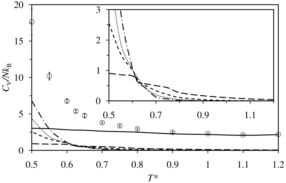
Figure 3: Canonical Monte Carlo (homogeneous, $N_{*}=N=5,000$) results for the specific heat capacity for Lennard-Jones ⁴He along the saturation curve. The symbols are the total of the monomer and loop contributions. The full curve is the monomer or classical contribution. The loop contribution curves are dimer (long dashed), trimer (short dashed), tetramer (dotted), and pentamer (dash-dotted). Each arm of an error bar is twice the standard error. Inset. Magnification of the loop contributions.

Figure 3 shows the simulated heat capacity for interacting bosons, namely helium-4 with Lennard-Jones pair interactions. Details of the Monte Carlo algorithm are given by Attard (2021 section 5.3.2). The difference between the present results and those reported by Attard (2021 section 5.3.3) is that the earlier results were for an inhomogeneous canonical system consisting of a liquid drop in equilibrium with its own vapor. The present results are for a homogenous canonical system at the saturated liquid density previously established at each temperature by the inhomogeneous simulation. Artifacts due to the fluctuations in the liquid drop that contribute significantly to the heat capacity for the total system reported by Attard (2021) are absent in Fig. 3. It can be seen that the magnitude of the heat capacity for the Lennard-Jones liquid is much larger than that of the ideal gas, Fig. 2, and comparable to that measured experimentally for ⁴He in the vicinity of the $\lambda$-transition (Donnelly and Barenghi 1998).

The individual loop contributions come from expressing the second temperature derivative of the loop grand potentials as classical averages (Attard 2021 section 5.3.1). It can be seen that for $T*\gtrsim 0.9$ the quantum contributions are negligible. For $0.6\lesssim T^{*}\lesssim 0.8$ the loop contributions increase with decreasing temperature, with the lower order loops having largest effect. At about $T^{*}=0.6$ the order of the loops flips, and the loop series appears divergent. This suggests that for the Lennard-Jones fluid the $\lambda$-transition occurs around about $T^{*}_{\mathrm{c}}\approx 0.6$, which for the usual Lennard-Jones parameters of helium-4 (van Sciver 2012) corresponds to $T_{\mathrm{c}}\approx 6$ K. (The temperature $T^{*}\approx 0.6$ also signals the onset of ground momentum state condensation, as shown by the results in sections IV.2 and IV.3 below.)

One should not be unduly concerned that this predicted $\lambda$-transition temperature differs from the measured one, $T_{\mathrm{c}}=$2.17 K (Donnelly and Barenghi 1998). The present Lennard-Jones parameters, $\varepsilon_{\mathrm{He}}=10.22k_{\mathrm{B}}$ J and $\sigma_{\mathrm{He}}=0.2556$ nm (van Sciver 2012) could be simply rescaled, $\varepsilon=0.43\varepsilon_{\mathrm{He}}$ and $\sigma=1.4\sigma_{\mathrm{He}}$, to bring the transition temperature and the saturation density into consonance with the measured values. The functional form of the Lennard-Jones pair potential, and the absence of many-body potentials, appear inadequate for a quantitatively accurate description of liquid helium at these low temperatures. The real message from Fig. 3 is that particle interactions play an essential role in the $\lambda$-transition and that this can be explored with computer simulations.

A second limitation of the simulation results in Fig. 3 is that they used classical canonical averages with $N$ bosons and the momentum continuum, $\langle\ldots\rangle_{N,\mathrm{cl}}$. This is valid if the number of bosons in the ground momentum state is negligible compared to the number of excited momentum state bosons, $N_{0}\ll N_{*}$. Such an assumption obviously breaks down after the $\lambda$-transition. In the unmixed case the primary correction for this effect is to multiply the energy due to an $l$-loop, $l\geq 2$, by $(\overline{N}_{*}/N)^{l}$, using an estimate of the optimum fraction of excited momentum state bosons at each temperature. This is done below the $\lambda$-transition in Fig. 1 and is discussed in §IV.4. If condensation increases continuously with decreasing temperature, as will now be shown in the unmixed case, such a correction reduces the heat capacity in Fig. 3 following the $\lambda$-transition.

Table 1: Intensive Gaussian loop $g^{(l)}=\langle G^{(l)}\rangle_{N,\mathrm{cl}}/N$ from liquid drop Monte Carlo simulations ($N=500$, $\rho\sigma^{3}=0.3$) for saturated Lennard-Jones He⁴ at various temperatures, $T^{*}\equiv k_{\mathrm{B}}T/\varepsilon$.

$l$	$T^{*}=1$	0.9	0.8	0.7
2	2.44E-03	5.59E-03	1.24E-02	2.70E-02
3	6.77E-05	2.81E-04	1.11E-03	4.25E-03
4	3.84E-06	2.60E-05	1.67E-04	1.06E-03
5	3.20E-07	3.28E-06	3.38E-05	3.57E-04
$l$	$T^{*}=0.6$	0.55	0.5	0.45
2	5.90E-02	8.72E-02	1.29E-01	1.96E-01
3	1.63E-02	3.20E-02	6.32E-02	1.33E-01
4	6.62E-03	1.68E-02	4.28E-02	1.30E-01
5	3.62E-03	1.19E-02	3.94E-02	1.56E-01
6	2.08E-03	8.76E-03	3.72E-02	2.24E-01

Using the mean field results of the previous section the number of ground momentum state bosons can be estimated. Table 1 gives the intensive Gaussian loop weights, $g^{(l)}\equiv\langle G^{(l)}({\bf q}^{N})\rangle_{N,\mathrm{cl}}/N$. These were obtained from the Monte Carlo simulations of Lennard-Jones ⁴He (Attard 2021). The statistical error was less than the displayed digits. It can be seen that the terms increase with decreasing temperature. At each temperature the terms decrease with increasing loop size, except possibly at the lowest temperature shown.

Table 2: Saturation density and fraction of ground momentum state bosons in Lennard-Jones He⁴. From liquid drop Monte Carlo simulations with $N_{*}=N=500$ at an overall density of $\rho\sigma^{3}=0.3$.

$k_{\mathrm{B}}T/\varepsilon$	$\rho\sigma^{3}$	$\rho\Lambda^{3}$	$T$ (K)†	$\rho_{\mathrm{m}}$ (kg m$\!{}^{-3}$)†	$\overline{N}_{0}/N$
1	0.62	0.76	10.220	246.76	0
0.9	0.73	1.04	9.198	290.54	0.027
0.8	0.77	1.31	8.176	306.46	0.220
0.7	0.81	1.68	7.154	322.38	0.381
0.6	0.88	2.31	6.132	350.24	0.536
0.55	0.87	2.60	5.621	346.26	0.583
0.5	0.91	3.13	5.110	366.16	0.635
0.45	0.95	3.82	4.599	376.91	0.682
0.4	0.98	4.72	4.088	390.04	0.709

^†$\varepsilon_{\mathrm{He}}=10.22k_{\mathrm{B}}$ J and $\sigma_{\mathrm{He}}=0.2556$ nm.

Table 2 shows the optimal fraction of bosons in the system that are in the ground momentum state as a function of temperature. The mean field theory, Eq. (3.13), was used together with the results in Table 1. The results represent the stable solutions. At $T^{*}=0.45$, changing $l_{\mathrm{max}}$ from 6 to 5 changes $\overline{N}_{0}/N$ from 0.682 to 0.684.

One can compare these results to the exact calculations for the ideal gas, Eq. (2.2). As reported in Attard (2021 section 5.2) for $N=500$ about 20% of the bosons are in the ground momentum state at the $\lambda$-transition. For $N=1000$ it is about 10%, and for $N=5000$ it is about 5%. In the thermodynamic limit the ideal gas apparently shows a continuous condensation transition, beginning with zero ground momentum state occupation at the transition itself, followed by a continuous increase in occupancy below the transition. In contrast, the present results for the Lennard-Jones liquid, Table 2, have a substantial fraction of bosons occupying the ground momentum state at the transition. The present mean field results indicate that the ground momentum state occupancy increases continuously through the transition. In the light of the following results for mixed permutation loops, this continuity appears to be an artefact of the no mixing approximation, whereas the non-zero value for ground momentum state occupancy at the condensation transition appears to be reliable.

IV Mixed Loops

In order to go beyond the mean field (i.e.  no mixing) approach one must include mixed permutation loops that contain both ground and excited momentum state bosons. Such mixed loops are essential because they provide the nucleating mechanism for ground momentum state condensation. Despite the strong inference based on the experimental and computational evidence that mixed loops nucleate condensation, their very existence poses a surprising conceptual and mathematical challenge.

For the ideal gas, only pure permutation loops are allowed: momentum states cannot be mixed in any one loop. The prohibition on mixing in the ideal gas is due to the orthogonality of the momentum eigenfunctions; the ideal gas configuration integral is the same as the expectation value integral. For interacting bosons this restriction does not apply directly because the interaction potential in the Maxwell-Boltzmann factor means that the configuration integral differs from the expectation value integral in which orthogonality would otherwise hold.

This observation might lead one to conclude that mixed ground and excited momentum permutation loops for interacting bosons are fully permitted. But closer inspection reveals a complication, namely that at large separations the interaction potential goes to zero, which means that the bosons behave ideally with respect to each other. From this point of view mixed ground and excited momentum state loops would be forbidden also for interacting bosons because the large separation regime dominates the configuration integral. There is an issue to be resolved here that turns on the form of the London (1938) approximation, the nature of generalized functions, and the order of integration.

In the discrete momentum picture,

$$\int_{V}\mathrm{d}{\bf q}_{12}\;e^{-{\bf p}_{12}\cdot{\bf q}_{12}/\mathrm{i}\hbar}=V\delta_{{\bf p}_{1},{\bf p}_{2}},$$ (4.1)

whereas in the continuum momentum picture

$$\int\mathrm{d}{\bf q}_{12}\;e^{-{\bf p}_{12}\cdot{\bf q}_{12}/\mathrm{i}\hbar}=(2\pi\hbar)^{3}\delta({\bf p}_{1}-{\bf p}_{2}).$$ (4.2)

In these Kronecker and Dirac $\delta$-functions respectively appear. Because of this difference, one can only apply the London approximation after performing the position integral for the particle density asymptote, as will be demonstrated.

IV.1 Mixed Dimer

In order to account for mixed permutation loops write the symmetrization function as

$$\eta({\bf q},{\bf p}) = \eta_{0}({\bf q}^{N_{0}},{\bf p}^{N_{0}})\eta_{*}({\bf q}^{N_{*}},{\bf p}^{N_{*}})$$ (4.3)

$$\mbox{ }\times\big{[}1+\eta_{\mathrm{mix}}({\bf q},{\bf p})\big{]}.$$

Here $\eta_{0}=N_{0}!$ is the pure ground momentum state symmetrization function, $\eta_{*}$ is the pure excited momentum state symmetrization function, and $\eta_{\mathrm{mix}}$ is the sum of mixed loop weights.

The ground momentum state bosons in any one mixed loop are inaccessible to $\eta_{0}$ and their number have to be removed from it. This is most easily done by fixing $\eta_{0}=N_{0}!$ and multiplying each mixed symmetrization loop with $n_{0}$ ground momentum state bosons by $(N_{0}-n_{0})!/N_{0}!$. The excited loops are compact, and so we can neglect any similar dependence on $n_{*}$ in the thermodynamic limit.

Here we focus on the leading mixed contribution, which is the mixed dimer,

$$\eta^{(1;1)}_{0*}({\bf q},{\bf p})=\sum_{j}^{N_{0}}\sum_{k}^{N_{*}}e^{-{\bf p}_{k}\cdot{\bf q}_{kj}/\mathrm{i}\hbar}.$$ (4.4)

This is also the dimer chain, $\tilde{\eta}^{(2)}$, and it belongs to the class of singly excited mixed loops, $\eta^{(n;1)}$, both of which are treated below. As mentioned, we can account for the fact that there are now $N_{0}-1$ ground momentum state bosons available for pure loops by dividing this by $N_{0}$, which will then leave $\eta_{0}=N_{0}!$ unchanged.

We suppose that we can factorize the classical average of the symmetrization function

$$\left\langle\eta_{0}\eta_{*}\eta^{(1;1)}_{0*}/N_{0}\right\rangle_{z,\mathrm{cl}}=\left\langle\eta_{0}\eta_{*}\right\rangle_{z,\mathrm{cl}}\;\left\langle\eta^{(1;1)}_{0*}/N_{0}\right\rangle_{z,\mathrm{cl}}.$$ (4.5)

The unmixed factor was dealt with above.

Using for convenience a canonical rather than a grand canonical average, in the discrete momentum case one can write for this

$$\left\langle\eta^{(1;1)}_{0*}/N_{0}\right\rangle_{N_{0},N_{*},\mathrm{cl}}$$ (4.6)

$$= \frac{\Lambda^{3N_{*}}}{V^{N_{*}}}\prod_{j}^{N_{0}}\delta_{{\bf p}_{j},{\bf 0}}\prod_{k}^{N_{*}}\sum_{{\bf p}_{k}}\!^{(p_{k}>0)}e^{-\beta p_{k}^{2}/2m}$$

$$\mbox{ }\times\left\langle\frac{1}{N_{0}}\sum_{j}^{N_{0}}\sum_{k}^{N_{*}}e^{-{\bf p}_{k}\cdot{\bf q}_{kj}/\mathrm{i}\hbar}\right\rangle_{N,\mathrm{cl}}$$

$$= \frac{\Lambda^{3N_{*}}}{V^{N_{*}}}\frac{N_{*}}{N(N-1)}\prod_{j}^{N_{0}}\delta_{{\bf p}_{j},{\bf 0}}\prod_{k}^{N_{*}}\sum_{{\bf p}_{k}}\!^{(p_{k}>0)}e^{-\beta p_{k}^{2}/2m}$$

$$\mbox{ }\times\int_{V}\mathrm{d}{\bf q}_{1}\,\mathrm{d}{\bf q}_{2}\,\rho^{(2)}_{N}({\bf q}_{1},{\bf q}_{2})e^{-{\bf p}_{1}\cdot{\bf q}_{12}/\mathrm{i}\hbar}.$$

The angular brackets represent the configurational average, the momentum average being explicit: the prefactor for the first equality is the normalization for the momentum states, which invokes the continuum integral for the excited states because in this case there is no issue with generalized functions. The second equality converts the configuration average to an integral over the canonical pair density, which is normalized as $\int_{V}\mathrm{d}{\bf q}_{1}\,\mathrm{d}{\bf q}_{2}\,\rho^{(2)}_{N}({\bf q}_{1},{\bf q}_{2})=N(N-1)$. In this case particle 1 is in an excited momentum state and particle 2 is in the momentum ground state, although this makes no difference to the configuration integral.

The asymptotic contribution to the configurational integral is

$$\rho^{2}\int_{V}\mathrm{d}{\bf q}_{1}\,\mathrm{d}{\bf q}_{2}\,e^{-{\bf p}_{1}\cdot{\bf q}_{12}/\mathrm{i}\hbar}=\rho^{2}V\delta_{{\bf p}_{1},{\bf 0}}=0.$$ (4.7)

Since $p_{1}>0$ by design, this vanishes. Therefore in order to transform the sum over excited states to the integral over the momentum continuum and interchange the order of integration we must first replace the pair density by its connected part,

$$\rho^{2}h^{(2)}_{N}({\bf q}_{1},{\bf q}_{2})=\rho^{(2)}_{N}({\bf q}_{1},{\bf q}_{2})-\rho^{2}.$$ (4.8)

Here we assume a homogeneous system, $\rho^{(1)}_{N}({\bf q}_{1})=\rho=N/V$, in which case the total correlation function depends upon the particle separation, $h^{(2)}_{N}({\bf q}_{1},{\bf q}_{2})=h^{(2)}_{N}(q_{12})$.

Subtracting the asymptote we are left with a short-ranged integrand and therefore no generalized function. Hence we may transform to the momentum continuum, interchange the order of integration, and perform the integral over the excited states. These give

$$\left\langle\eta^{(1;1)}_{0*}/N_{0}\right\rangle_{N_{0},N_{*},\mathrm{cl}}$$ (4.9)

$$= \frac{\Lambda^{3N_{*}}}{V^{N_{*}}}\frac{N_{*}}{N(N-1)}\prod_{j}^{N_{0}}\delta_{{\bf p}_{j},{\bf 0}}\prod_{k}^{N_{*}}\sum_{{\bf p}_{k}}\!^{(p_{k}>0)}e^{-\beta p_{k}^{2}/2m}$$

$$\mbox{ }\times\int\mathrm{d}{\bf q}_{1}\,\mathrm{d}{\bf q}_{2}\,\rho^{2}h^{(2)}_{N}({\bf q}_{1},{\bf q}_{2})e^{-{\bf p}_{1}\cdot{\bf q}_{12}/\mathrm{i}\hbar}$$

$$= \frac{\Lambda^{3N_{*}}}{V^{N_{*}}}\frac{N_{*}}{N(N-1)}\Delta_{p}^{-3N_{*}}\int\mathrm{d}{\bf p}^{N_{*}}\;e^{-\beta{\cal K}({\bf p}^{N_{*}})}$$

$$\mbox{ }\times\int\mathrm{d}{\bf q}_{1}\,\mathrm{d}{\bf q}_{2}\;\rho^{2}h^{(2)}_{N}({\bf q}_{1},{\bf q}_{2})e^{-{\bf p}_{1}\cdot{\bf q}_{12}/\mathrm{i}\hbar}$$

$$= \frac{\rho^{2}N_{*}}{N(N-1)}\int\mathrm{d}{\bf q}_{1}\,\mathrm{d}{\bf q}_{2}\;h^{(2)}_{N}({\bf q}_{1},{\bf q}_{2})e^{-\pi q^{2}_{12}/\Lambda^{2}}$$

$$= \frac{N_{*}}{V}\int\mathrm{d}{\bf q}_{12}\,h^{(2)}_{N}(q_{12})e^{-\pi q_{12}^{2}/\Lambda^{2}}.$$

This can also be written

$$\left\langle\eta^{(1;1)}_{0*}/N_{0}\right\rangle_{N_{0},N_{*},\mathrm{cl}}$$ (4.10)

$$= \frac{N_{*}V}{N^{2}}\int\mathrm{d}{\bf q}_{12}\;\rho^{(2)}_{N}(q_{12})e^{-\pi q_{12}^{2}/\Lambda^{2}}-\frac{N_{*}V}{N^{2}}\rho^{2}\Lambda^{3}$$

$$= \frac{N_{*}}{N}\left\langle\frac{2}{N}\sum_{j<k}^{N}e^{-\pi q_{jk}^{2}/\Lambda^{2}}\right\rangle_{N,\mathrm{cl}}-\frac{N_{*}V}{N^{2}}\rho^{2}\Lambda^{3}$$

$$= \frac{N_{*}}{N}\left\langle\frac{1}{N}\sum_{j,k}^{N}\!{}^{\prime}\left[e^{-\pi q_{jk}^{2}/\Lambda^{2}}-\frac{\rho\Lambda^{3}}{N}\right]\right\rangle_{N,\mathrm{cl}}$$

$$\equiv \frac{N_{*}}{N}\left\langle\tilde{\eta}^{(2)}/N\right\rangle_{N,\mathrm{cl}}^{\mathrm{corr}}.$$

The final average, which is in a canonical classical system of $N$ particles, has the asymptotic correction as defined by the preceding equality. The result is intensive.

For high temperatures $\Lambda\lesssim\sigma$, which means that the integral vanishes in the core, $\rho^{(2)}_{N}(q_{12})=0$, $q_{12}\lesssim\sigma$. Hence at high temperatures $\langle\eta^{(1;1)}_{0*}/N_{0}\rangle_{N_{0},N_{*},\mathrm{cl}}\sim-\rho\Lambda^{3}$. That this is negative means that such mixed dimers are entropically unfavorable in this regime, which suppresses ground momentum state occupation, which will turn out to be significant.

IV.2 Singularly Exciting Mixed Loops

IV.2.1 Analysis

Consider mixed $l$-loops with one excited momentum state boson, labeled 1 or $j_{1}$, and $l-1$ ground momentum state bosons, labeled $2,\ldots,l$ or $k_{2},\ldots,k_{l}$, whose weight we shall denote as $\eta^{(l-1;1)}_{0*}$. A particular such loop with particle 1 excited has symmetrization factor $e^{-{\bf p}_{1}\cdot{\bf q}_{12}/\mathrm{i}\hbar}$, which is independent of the positions of all the ground momentum state bosons in the loop, ${\bf q}_{3},{\bf q}_{4},\ldots,{\bf q}_{l-1}$, except the adjacent one labeled 2. Therefore we can arrange them in $(l-2)!$ ways without changing the value of the symmetrization factor. The total weight involving all such singly excited mixed loops is

$$\eta_{0}\,\eta_{*}\eta^{(l-1;1)}_{0*}$$ (4.11)

$$= (N_{0}-l+1)!\,\eta_{*}(N_{*})\sum_{k_{2},\ldots,k_{l}}^{N_{0}}\!\!\!{}^{\prime}\;\sum_{j_{1}}^{N_{*}}e^{-{\bf p}_{j_{1}}\cdot{\bf q}_{j_{1},k_{2}}/\mathrm{i}\hbar}$$

$$= (N_{0}-l+1)!\,\eta_{*}(N_{*})\frac{(N_{0}-1)!}{(N_{0}-l+1)!}$$

$$\mbox{ }\times\sum_{k_{2}}^{N_{0}}\sum_{j_{1}}^{N_{*}}e^{-{\bf p}_{j_{1}}\cdot{\bf q}_{j_{1},k_{2}}/\mathrm{i}\hbar}$$

$$= \eta_{0}(N_{0})\,\eta_{*}(N_{*})\frac{1}{N_{0}}\sum_{k_{2}}^{N_{0}}\sum_{j_{1}}^{N_{*}}e^{-{\bf p}_{j_{1}}\cdot{\bf q}_{j_{1},k_{2}}/\mathrm{i}\hbar}.$$

The mixed factor is obviously intensive (i.e. independent of $N_{0}$ and of $N_{*}$) in the thermodynamic limit, since for each ground momentum state boson there is a limited number of excited momentum state bosons in the neighborhood that will give a non-zero weight after averaging.

The singularly excited mixed loop phase function defined by the final equality here, $\eta^{(l-1;1)}_{0*}({\bf q},{\bf p})$, is identical to the mixed dimer phase function, Eq. (4.4). Hence its average is also the same. Importantly, it is independent of $l$, which means that their total contribution is

$$-\beta\Omega_{\mathrm{mix}}^{(1)} = \sum_{l=2}^{N_{0}+1}\left\langle\eta^{(l-1;1)}_{0*}/N_{0}\right\rangle_{N_{0},N_{*},\mathrm{cl}}$$ (4.12)

$$= N_{0}\left\langle\eta^{(1;1)}_{0*}/N_{0}\right\rangle_{N_{0},N_{*},\mathrm{cl}}$$

$$= \frac{N_{0}N_{*}}{N}\left\langle\tilde{\eta}^{(2)}/N\right\rangle_{N,\mathrm{cl}}^{\mathrm{corr}},$$

where the final factor on the right hand side is given in Eq. (4.10). This is the total from all mixed symmetrization loops that have a single excited momentum state boson.

One can write the grand potential as $\Omega=\Omega_{\mathrm{cl}}+\Omega_{*}+\Omega_{\mathrm{mix}}$, with the first two terms being given by Eqs (3.10) and (3.11), respectively. The present $\Omega_{\mathrm{mix}}^{(1)}$ is the leading order contribution to the mixed term. Its derivative at constant $N$ is

$$\left(\frac{\partial(-\beta\Omega_{\mathrm{mix}}^{(1)})}{\partial N_{*}}\right)_{N}=\frac{N-2N_{*}}{N}\left\langle\tilde{\eta}^{(2)}/N\right\rangle_{N,\mathrm{cl}}^{\mathrm{corr}}.$$ (4.13)

The average is independent of $N_{*}$. The prefactor is negative for $N_{*}>N/2$, which is the case at high temperatures. As mentioned above the average of the mixed dimer must be negative for high temperatures. These two facts means that at high temperatures this derivative is positive, which increases the occupation of the excited states compared to the classical and pure terms alone.

IV.2.2 Numerical Results

Table 3: Liquid density, mixed dimer weight, and optimum ground momentum state fraction for saturated Lennard-Jones He⁴ at various temperatures, $T^{*}\equiv k_{\mathrm{B}}T/\varepsilon$. From liquid drop Monte Carlo simulations with $N=5000$, overall density of $\rho\sigma^{3}=0.2$, using the central liquid volume of radius $10\sigma$ for the averages.

$T^{*}$	$\rho\sigma^{3}$	$\rho\Lambda^{3}$	$\displaystyle\frac{\langle\tilde{\eta}^{(2)}\rangle_{N,\mathrm{cl}}^{\mathrm{corr}}}{N}$	$\displaystyle\frac{\overline{N}_{0}}{N}$	$\displaystyle\frac{\overline{N}_{0}}{N}$
				stable	unstable
1.00	0.67	0.81	-0.60	0	-
0.90	0.73	1.05	-0.70	0	-
0.80	0.79	1.34	-0.79	0	-
0.70	0.83	1.73	-0.87	0	-
0.65	0.86	1.99	-0.90	0	-
0.60	0.88	2.29	-0.93	0.640	0.35
0.55	0.90	2.67	-0.96	0.754	0.35
0.50	0.91	3.14	-0.99	0.818	0.35
0.45	0.97	3.93	-1.04	0.872	0.45
0.40	0.99	4.74	-1.06	0.902	0.55

Simulation results for the mixed dimer are shown in Table 3. The difference in the Lennard-Jones saturation density compared to that in Table 2 is partly due to the larger system size and lower overall density here, which means that the periodic boundary conditions have less influence on the shape of the liquid phase. The primary difference is that here the averages were taken over a sphere of radius $10\sigma$ about the center of mass, whereas in Table 2 they were taken over the whole system, of which approximately 20% of the bosons were in the vapor phase or interfacial region. For the present larger system at $T^{*}=0.5$, the radius of the interface at half density is $\approx 10.6\sigma$. The central density measured within $2\sigma$ of the center of mass is $\rho\sigma^{3}=0.943(1)$, whereas the density measured within $10\sigma$ is $\rho\sigma^{3}=0.9116(5)$. For $T^{*}\lesssim 0.5$ the system was somewhat glassy, with limited or no macroscopic diffusion of the particles.

It can be seen in Table 3 that the mixed dimer weight is negative at all temperatures. This means that the asymptotic correction dominates. The weight increases in magnitude with decreasing temperature, although the dependence on temperature is rather weak.

The mixed dimer weight was combined with the classical pure loop grand potential, $\Omega=\Omega_{\mathrm{cl}}+\Omega_{\mathrm{pure}}+\Omega_{\mathrm{mix}}^{(1)}$, with the first two terms being given by Eqs (3.10) and (3.11), and the singly excited mixed grand potential by Eq. (4.12). The pure loops used $l_{\mathrm{max}}=4$ for $T^{*}\geq 0.7$ and $l_{\mathrm{max}}=5$ for $T^{*}\leq 0.65$. The results were little different when $l_{\mathrm{max}}$ was increased by one. The optimum fraction of bosons in the ground momentum state, $\overline{N}_{0}/N$, corresponds to the vanishing of the derivative of the grand potential, Eq. (3.13) plus Eq. (4.13). It can be seen in Table 3 that for $T^{*}\geq 0.65$ there is only one stable solution, namely all the bosons in the system are in excited states. For temperatures $T^{*}\leq 0.6$ (6.13 K), there are two zeros for the derivative, the higher fraction being the stable solution (i.e. the minimum in the grand potential). At $T^{*}=0.6$ the stable fraction of ground momentum state bosons is $\overline{N}_{0}/N=0.640$, which is a rather abrupt change from $\overline{N}_{0}/N=0$ at $T^{*}=0.65$. It would be fair to call this ground momentum state condensation. The transition more or less coincides with the passage of $\overline{N}_{0}/N$ from greater than one half to less than one half, as given by the pure loops only in Table 2. The value $\overline{N}_{0}/N=0.640$ obtained by including the mixed dimer is greater than the value $\overline{N}_{0}/N=0.536$ in Table 2 obtained with the pure loops only, as is expected for a negative values of $\langle\tilde{\eta}^{(2)}\rangle_{N,\mathrm{cl}}^{\mathrm{corr}}$.

In Table 3 it can be seen that $\langle\tilde{\eta}^{(2)}\rangle_{N,\mathrm{cl}}^{\mathrm{corr}}/N>-1$ for $T^{*}>0.45$. Obviously there is some uncertainty in where it first exceeds this bound as it is the difference between two positive comparable quantities, and it therefore has a larger relative error than either alone. Minus one is significant because it marks the point, at the dimer level of approximation, $1+(N_{*}/N)\langle\tilde{\eta}^{(2)}\rangle_{N,\mathrm{cl}}^{\mathrm{corr}}/N$, beyond which it is not possible to have a fully excited system, $\overline{N}_{*}/N=1$ (c.f. dressed bosons below).

In any case the present mixed loop calculations provide a credible mechanism for ground momentum state condensation. Compared to the unmixed results, Table 2, where the condensation grows continuously from zero at $\rho\Lambda^{3}=1$, in the mixed case the condensation is rather sudden, and it occurs at $\rho\Lambda^{3}=2.29$. Since mixed loops are forbidden in the ideal gas this effect is specific to interacting bosons. It shows that the growth of excited state position permutation loops nucleate, or are responsible for, ground momentum state condensation (Attard 2021 section 5.6.1.7).

IV.3 Dressed Bosons

In the preceding subsection the non-local nature of the ground momentum state was exploited to incorporate an arbitrary number of ground momentum state bosons into the mixed dimer permutation loop to obtain the so-called singly excited grand potential as the leading order contribution from mixed ground and excited momentum state permutation loops. In this subsection this idea is generalized to form mixed permutation loops by concatenating permutation chains, which consist of a ground momentum state boson as the head and excited momentum state bosons as the tail. The series of such chains may be called a dressed ground momentum state boson, or dressed boson for short. The theory based on them is like the ideal solution theory of physical chemistry, with the dressed ground momentum state bosons being the solute that forms a dilute solution in the fluid of excited momentum state bosons.

Consider a $l$-chain, with the ground momentum state boson at the head, which we designate as position $l$, and with $l-1$ excited momentum state bosons forming the tail. A particular chain has symmetrization function

$$\tilde{\eta}^{(l)}_{j_{1},\ldots,j_{l}}$$

$$= e^{-{\bf p}_{j_{1}}\cdot{\bf q}_{j_{1},j_{2}}/\mathrm{i}\hbar}e^{-{\bf p}_{j_{2}}\cdot{\bf q}_{j_{2},j_{3}}/\mathrm{i}\hbar}\ldots e^{-{\bf p}_{j_{l-1}}\cdot{\bf q}_{j_{l-1},j_{l}}/\mathrm{i}\hbar}.$$

The sum of all possible dimer chains is the same as the mixed dimer symmetrization function, Eq. (4.4),

$$\eta^{(1;1)}_{0*}({\bf q},{\bf p}) = \sum_{j}^{N_{0}}\sum_{k}^{N_{*}}e^{-{\bf p}_{k}\cdot{\bf q}_{kj}/\mathrm{i}\hbar}$$ (4.15)

$$= \sum_{j}^{N_{0}}\sum_{k}^{N_{*}}\tilde{\eta}^{(2)}_{k,j}.$$

The average of this correcting for the asymptote is given as Eq. (4.10).

The sum of all possible trimer chains is the same as the mixed trimer symmetrization function with one ground and two excited momentum state bosons, Eq. (A.1),

$$\eta^{(1;2)}_{0*}({\bf q},{\bf p}) = \sum_{j}^{N_{0}}\sum_{k,l}^{N_{*}}\!{}^{\prime}\;e^{-{\bf p}_{k}\cdot{\bf q}_{kl}/\mathrm{i}\hbar}e^{-{\bf p}_{l}\cdot{\bf q}_{lj}/\mathrm{i}\hbar}$$ (4.16)

$$= \sum_{j}^{N_{0}}\sum_{k,l}^{N_{*}}\!{}^{\prime}\;\tilde{\eta}^{(3)}_{k,l,j}.$$

The prime on the sum indicates that no two indeces may be equal. The average of this correcting for the asymptote is given as Eq. (A.5).

For a ground state boson $k$, chains of a given length may be summed over all excited momentum state bosons,

$$\tilde{\eta}^{(l)}_{k}({\bf q},{\bf p})=\sum_{j_{1},\ldots,j_{l-1}}^{N_{*}}{}^{\prime}\hskip 8.5359pt\tilde{\eta}^{(l)}_{j_{1},\ldots,j_{l-1},k}({\bf q},{\bf p}).$$ (4.17)

These in turn may be summed over all lengths

$$\tilde{\eta}_{k}({\bf q},{\bf p})=\sum_{l=2}^{N_{*}+1}\tilde{\eta}^{(l)}_{k}({\bf q},{\bf p}).$$ (4.18)

The quantity $\tilde{\eta}_{k}({\bf q},{\bf p})$ is the symmetrization weight of the dressed ground momentum state boson $k$ at this point in phase space. We may average this weight, either before or after summing over chain length, and treat the dressed ground momentum state bosons as independent, which is valid if they are dilute compared to the excited momentum state bosons, $N_{0}(l_{\mathrm{max}}-1)\ll N_{*}$.

One can form $N_{0}!$ permutations of the dressed bosons. But for this to work one needs to show that the weight upon concatenation of two chains into a permutation loop is the same as the product of the weights of the two individual permutation chains. To this end, consider an $l$-chain $j_{1},j_{2},\ldots,j_{l}$ and an $m$-chain, $k_{1},k_{2},\ldots,k_{m}$. The symmetrization function for the permutation loop formed from them is

$$\tilde{\eta}^{(l+m)}_{j^{l},k^{m}}({\bf q},{\bf p})$$ (4.19)

$$= e^{-{\bf p}_{j_{1}}\cdot{\bf q}_{j_{1},j_{2}}/\mathrm{i}\hbar}\ldots e^{-{\bf p}_{j_{l-1}}\cdot{\bf q}_{j_{l-1},j_{l}}/\mathrm{i}\hbar}$$

$$\mbox{ }\times e^{-{\bf p}_{k_{1}}\cdot{\bf q}_{k_{1},k_{2}}/\mathrm{i}\hbar}\ldots e^{-{\bf p}_{k_{m-1}}\cdot{\bf q}_{k_{m-1},k_{m}}/\mathrm{i}\hbar}$$

$$= \tilde{\eta}^{(l)}_{j^{l}}({\bf q},{\bf p})\,\tilde{\eta}^{(m)}_{k^{m}}({\bf q},{\bf p}).$$

The two transposition factors that link the chains, $e^{-{\bf p}_{j_{l}}\cdot{\bf q}_{j_{l},k_{1}}/\mathrm{i}\hbar}$ and $e^{-{\bf p}_{k_{m}}\cdot{\bf q}_{k_{m},j_{1}}/\mathrm{i}\hbar}$, are unity because the head bosons are in the ground momentum state, ${\bf p}_{j_{l}}={\bf p}_{k_{m}}={\bf 0}$. Hence the permutation loop function formed by concatenating the two chains is just the product of the two chain functions, with the restriction that no index can be the same. Since the chains are compact, and since it is assumed that $N_{0}\ll N_{*}$ (dilute solution), this restriction can be dropped with negligible error. From this it follows that the $N_{0}!$ permutations of particular chains form legitimate permutation loops, and that all $N_{0}!$ permutations have the same total weight, which is equal to the product of the weights of the individual chains.

The average weight of a dressed ground momentum state boson is

$$\left\langle\tilde{\eta}({\bf q},{\bf p})\right\rangle_{N_{0},N_{*},\mathrm{cl}} = \left\langle\frac{1}{N_{0}}\sum_{k}^{N_{0}}\tilde{\eta}_{k}({\bf q},{\bf p})\right\rangle_{N_{0},N_{*},\mathrm{cl}}$$ (4.20)

$$= \sum_{l=2}^{\infty}\left\langle\frac{1}{N_{0}}\sum_{k}^{N_{0}}\tilde{\eta}_{k}^{(l)}({\bf q},{\bf p})\right\rangle_{N_{0},N_{*},\mathrm{cl}}$$

$$= \sum_{l=2}^{\infty}\frac{N_{*}^{l-1}}{N^{l}}\left\langle\tilde{G}^{(l)}\right\rangle_{N,\mathrm{cl}}^{\mathrm{corr}}$$

$$= \sum_{l=2}^{\infty}\frac{N_{*}^{l-1}}{N^{l-1}}\tilde{g}^{(l)}.$$

The $l=2$ term is the mixed dimer, Eq. (4.10), and the $l=3$ term is the mixed trimer, Eq. (A.6). The chain Gaussian is

$$\tilde{G}^{(l)}({\bf q}^{N}) = \sum_{j_{1},\ldots,j_{l}}^{N}{}^{\prime}\hskip 2.84544pt\prod_{k=1}^{l-1}e^{-\pi q_{j_{k},j_{k+1}}/\Lambda^{2}}.$$ (4.21)

The prime indicates that no two indeces may be equal.

The product of the dressed weights of all the bosons gives the mixed grand partition function,

$$\tilde{\Xi}=1+\eta_{\mathrm{mix}}=\big{[}1+\langle\tilde{\eta}({\bf q},{\bf p})\rangle_{N_{0},N_{*},\mathrm{cl}}\big{]}^{N_{0}},$$ (4.22)

where the bare boson (monomer chain), $\tilde{\eta}^{(1)}=1$, appears explicitly. The logarithm gives the mixed grand potential

$$-\beta\tilde{\Omega}=N_{0}\ln\big{[}1+\langle\tilde{\eta}({\bf q},{\bf p})\rangle_{N_{0},N_{*},\mathrm{cl}}\big{]}.$$ (4.23)

The total grand potential is $\Omega=\Omega_{\mathrm{cl}}+\Omega_{*}+\tilde{\Omega}$. Implicitly, $N_{0}=\overline{N}_{0}(z,V,T)$ and $N_{*}=\overline{N}_{*}(z,V,T)$, although as a variational formulation this is a second order effect. The $N_{0}!$ permutations of the chains, which is the pure ground momentum state symmetrization weight, cancels with the same factor in the denominator of the partition function. The total weight of the ground momentum state bosons is the product of their average dressed weight, assuming that they do not overlap.

If one linearizes the expression for the mixed grand potential one obtains

$$-\beta\tilde{\Omega} = N_{0}\sum_{l=2}^{\infty}\left\langle\frac{1}{N_{0}}\sum_{k}^{N_{0}}\tilde{\eta}_{k}^{(l)}({\bf q},{\bf p})\right\rangle_{N_{0},N_{*},\mathrm{cl}}$$ (4.24)

$$= N_{0}\sum_{l=2}^{\infty}\frac{N_{*}^{l-1}}{N^{l-1}}\tilde{g}^{(l)}$$

$$= -\beta\sum_{l=2}^{\infty}\Omega_{\mathrm{mix}}^{(l-1)}.$$

The dimer term is just Eq. (4.12) and the trimer term is just Eq. (A.7). This shows how the present dressed boson theory is the non-linear generalization of the singly and doubly excited loops of section IV.1 and appendix A.

The derivative of the non-linear mixed grand potential is

$$\left(\frac{\partial\big{(}\beta\tilde{\Omega}\big{)}}{\partial N_{*}}\right)_{N} = -\ln\left[1+\sum_{l=2}^{\infty}\frac{N_{*}^{l-1}}{N^{l-1}}\tilde{g}^{(l)}\right]$$ (4.25)

$$\mbox{ }+\frac{\displaystyle\frac{N_{0}}{N}\sum_{l=2}^{\infty}(l-1)\frac{N_{*}^{l-2}}{N^{l-2}}\tilde{g}^{(l)}}{\displaystyle 1+\sum_{l=2}^{\infty}\frac{N_{*}^{l-1}}{N^{l-1}}\tilde{g}^{(l)}}.$$

Add this to the unmixed result, Eq. (3.13), to obtain the fraction of excited momentum state bosons in the system. One can also linearize this.

Table 4: Chain weights, $\tilde{g}^{(l)}=\langle\tilde{\eta}^{(l)}\rangle_{N,\mathrm{cl}}^{\mathrm{corr}}/N$, and optimum fraction of ground momentum state bosons for saturated Lennard-Jones He⁴ at various temperatures.

$T^{*}$	$\displaystyle\frac{\langle\tilde{\eta}\!^{(2)}\rangle_{N,\mathrm{cl}}^{\mathrm{corr}}}{N}$	$\displaystyle\frac{\langle\tilde{\eta}\!^{(3)}\rangle_{N,\mathrm{cl}}^{\mathrm{corr}}}{N}$	$\displaystyle\frac{\langle\tilde{\eta}\!^{(4)}\rangle_{N,\mathrm{cl}}^{\mathrm{corr}}}{N}$	$\displaystyle\frac{\overline{N}_{0}}{N}$	$\displaystyle\frac{\overline{N}_{0}}{N}$
				linear	non-linear
1.00	-0.599	0.357	-0.213	0	0
0.90	-0.700	0.486	-0.339	0	0
0.80	-0.790	0.613	-0.485	0	0
0.70	-0.866	0.728	-0.650	0	0
0.65	-0.904	0.782	-0.754	0	0.527
0.60	-0.934	0.820	-0.875	0.560	0.658
0.55	-0.963	0.852	-1.058	0.677	0.745
0.50	-0.992	0.889	-1.398	0.771	0.812
0.45	-1.038	1.089	-2.496	0.845	0.868
0.40	-1.063	1.180	-4.069	0.887	0.900

Table 4 shows results for chains up to $l_{\mathrm{max}}=4$. That the chain weights alternate in sign poses convergence problems. For $T^{*}\lesssim 0.55$ it is not clear that the chain series is converging (although of course each term must be multiplied by $(N_{*}/N)^{l-1}$). Retaining the first four terms in the series (including the monomer term of unity) gives a result for the optimum fraction of ground momentum state bosons in broad agreement with those predicted retaining two terms only, Table 3. The suppression of the occupation of the ground momentum state for $T^{*}\geq 0.65$ is likewise clear in the two tables. There is little difference between the linear and non-linear results, which perhaps suggests that the linear theory is exact. The location of the condensation, $T^{*}=0.6$, $\rho\Lambda^{3}=2.29$, is relatively insensitive to the level of the theory.

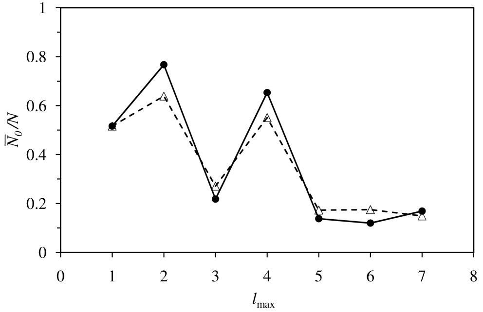
Figure 4: Fraction of ground momentum state bosons as a function of maximum chain length at $T^{*}=0.6$. The circles are non-linear results and the triangles are linear results, with the lines being an eye-guide. The unmixed excited momentum state loops used $l_{\mathrm{max}}=7$ in all cases. The statistical error is on the order of 1%.

Figure 4 shows the optimum fraction of ground momentum state bosons as a function of the maximum chain length at $T^{*}=0.6$. There is clearly an even/odd effect for $l_{\mathrm{max}}\leq 5$, but for larger values the fraction appears to have converged to $\overline{N}_{0}/N\approx 0.15$. Condensation appears to have occurred by $T^{*}=0.6$, although for individual choices of $l_{\mathrm{max}}$ it can occur by $T^{*}=0.65$ (c.f. Table 4 for $l_{\mathrm{max}}=4$, non-linear).

Similar behavior as a function of $l_{\mathrm{max}}$ occurred for $T^{*}=$ 0.62, 0.60, and 0.55. Condensation had occurred for almost all $l_{\mathrm{max}}$, linear and non-linear; the two exceptions in the 42 cases calculated happened at low $l_{\mathrm{max}}$. Using $l_{\mathrm{max}}=7$, the following ground momentum state bosons fractions were found: For $T^{*}=0.62$, ${\overline{N}_{0}}/{N}=$ 0.1480(3) (linear) and 0.1577(18) (non-linear). For $T^{*}=0.6$ , ${\overline{N}_{0}}/{N}=$ 0.1487(7) (linear) and 0.1695(23) (non-linear). And for $T^{*}=0.55$ ${\overline{N}_{0}}/{N}=$ 0.1405(4) (linear) and 0.1981(14) (non-linear). Since the change in the condensed fraction over these temperature intervals is negligible compared to the change from zero at $T^{*}=0.65$, one can conclude that the condensation transition is discontinuous. The transition occurs somewhere in the range $0.62\leq T_{\mathrm{c}}^{*}<0.65$.

IV.4 Energy and Heat Capacity in the Condensed Regime

In these results there is either no increase or else a slow increase in the fraction of ground momentum state bosons with decreasing temperature after the transition. The slowness of the increase appears to be an artefact that arises from assuming that the dressed bosons do not interfere with each other. The condition for non-interference, $N_{0}(l_{\mathrm{max}}-1)\ll N_{*}$, holds barely if at all in the present case; the left hand side is, say, $5\times 0.15=0.75$, whereas the right hand side is $0.85$. If interference were taken into account the contribution from mixed loops would be reduced (because many loops currently counted would be prohibited). Since the mixed loop contribution suppresses the number of ground momentum state bosons compared to the pure loop prediction, Table 2, interference between the mixed loops would reduce their negative contribution and hence increase the number of ground momentum state bosons above that calculated in the preceding paragraph. This means that the pure loop result becomes increasingly accurate below the condensation transition, as is its prediction that the ground momentum state is increasingly occupied as the temperature is decreased, Table 2.

This discussion leads to the conclusion that the mixed loop theory, linear or non-linear, is probably accurate for predicting the location of the condensation transition, but that it underestimates the number of ground momentum state bosons, and its rate of increase with decreasing temperature, once condensation has occurred. The pure loop theory is likely more accurate in the condensed regime. In calculating the effect of condensation on the energy and on the heat capacity, our strategy will be to use the mixed loop theory to locate the transition, and the pure loop theory to estimate the number of ground momentum state bosons in the condensed regime.

The average energy is the sum of loop energies, $\overline{\cal H}=\sum_{l=1}^{\infty}\overline{E}^{(l)}$. The averages are classical. One can relate each average loop energy for a system of $\overline{N}_{0}$ ground momentum state bosons and $\overline{N}_{*}=N-\overline{N}_{0}$ excited momentum state bosons, $\overline{E}^{(l)}\!(\overline{N}_{0},\overline{N}_{*})$, to one obtained in a classical system of $N$ bosons, $\overline{E}^{(l)}\!(N)$, as follows. The classical or monomer contribution is the sum of the classical kinetic energy and the potential energy,

$$\overline{E}^{(1)}\!(\overline{N}_{0},\overline{N}_{*})=\frac{3}{2}\overline{N}_{*}k_{\mathrm{B}}T+\left\langle U\right\rangle_{N,V,T}^{\mathrm{cl}}.$$ (4.26)

Obviously only excited momentum state bosons contribute to the kinetic energy. The potential energy does not distinguish ground and excited momentum state bosons. The dimer and higher loop energies are

$$\overline{E}^{(l)}\!(\overline{N}_{0},\overline{N}_{*})=\left(\frac{\overline{N}_{*}}{N}\right)^{l}\overline{E}^{(l)}\!(N),\;\;l\geq 2.$$ (4.27)

Above the condensation transition, $\overline{N}_{*}=N$ and the two systems are the same.

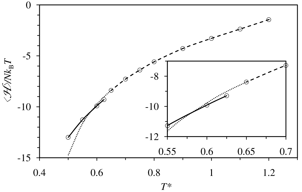
Figure 5: Canonical Monte Carlo (homogeneous, $N=5,000$) results for the average energy for Lennard-Jones He⁴ along the saturation curve using $l_{\mathrm{lmax}}=5$. The dashed and dotted curves use $N_{*}=N$, whereas the solid curve uses $\overline{N}_{0}$ given by the pure loop theory with $l_{\mathrm{max}}=7$. The error bars, whose total length is four times the standard statistical error, are less than the size of the symbols. Inset. Focus on the transition.

The average energy resulting from these formulae is shown in Fig. 5. These data resulted from homogeneous canonical Monte Carlo simulations along the saturated density curve. The condensation transition was set at $T_{\mathrm{c}}^{*}=0.625$, as determined by the mixed loop theory described in the preceding subsection. The fraction of ground momentum state bosons below the condensation transition was determined by the unmixed theory of section III.2 at the heptamer level of approximation. One can see in Fig. 5 that the condensed branch energy (solid curve) does not coincide with the non-condensed branch extrapolated to lower temperatures (dotted curve). At the highest condensed temperature in the figure, $T^{*}=0.625$, the value of the extrapolated energy that neglects the difference between ground and excited momentum state bosons is $\beta\langle{\cal H}\rangle/N=-9.017(2)$, whereas the actual condensed energy is $-9.295$. Hence the latent heat for the Lennard-Jones condensation transition is $E_{\mathrm{latent}}=0.3Nk_{\mathrm{B}}T$, which is 3% of the total energy. This surprisingly small value results from three effects: First, the kinetic energy, which is positive, is lower in magnitude in the condensed regime. Second, the loop energies, which are negative, are also lower in magnitude in the condensed regime. And third, the classical potential energy, $\beta\overline{U}^{(1)}/N=-9.958(1)$, which is 90% of the total, is unchanged. Because at the transition the fraction of ground momentum bosons is on the order of 50% (according to the unmixed theory), each individual change in energy is large relative to its contribution to the total. But their relative contribution to the total is only about 10%, and the two changes partially cancel each other. This leaves a residual latent heat of 3% of the total energy.

The heat capacity, which is the temperature derivative of the energy, can be similarly analyzed. The monomer term is

$$C_{\mathrm{V}}^{(1)}(\overline{N}_{0},\overline{N}_{*})=\frac{3\overline{N}_{*}k_{\mathrm{B}}}{2}+\frac{3k_{\mathrm{B}}T}{2}\frac{\partial\overline{N}_{*}}{\partial T}+C_{\mathrm{V}}^{\mathrm{cl,ex}}(N).$$ (4.28)

The dimer and higher loops contribute

$$C_{\mathrm{V}}^{(l)}(\overline{N}_{0},\overline{N}_{*}) = l\left(\frac{\overline{N}_{*}}{N}\right)^{l-1}\frac{\partial\overline{N}_{*}}{N\partial T}\overline{E}^{(l)}\!(N)$$ (4.29)

$$\mbox{ }+\left(\frac{\overline{N}_{*}}{N}\right)^{l}C_{\mathrm{V}}^{(l)}(N),\;\;l\geq 2.$$

The results are plotted in Fig. 1. The data are from homogeneous canonical Monte Carlo simulations at the saturated density. The difference with Fig. 3 is that those results are $C_{V}(N)$, which assume that all $N$ bosons are excited, whereas the results in Fig. 1 are $C_{\mathrm{V}}(\overline{N}_{0},\overline{N}_{*})$, which take into account the number of ground momentum state bosons given by the pure loop theory below the condensation transition given by the mixed loop theory. The qualitative and quantitative resemblance to the measured $\lambda$-transition in liquid helium-4 is unmistakable.

The above evidence that the condensation transition for interacting bosons is discontinuous is important. Of course prior to condensation the number of ground momentum state bosons is sub-extensive. Any finite value for the fraction at the transition indicates that the number of ground momentum state bosons has become extensive and it represents macroscopic condensation. The present results show that the system goes discontinuously from a sub-extensive (i.e. microscopic) to an extensive (i.e. macroscopic) number of ground momentum state bosons at the condensation transition. This contrasts with the ideal gas, where, in the thermodynamic limit, the number of ground momentum state bosons appears to grow continuously from zero at the condensation transition (c.f. the discussion following Table 2).

Although this observation provides a way of reconciling the experimental facts that the superfluid and the $\lambda$-transition are coincident, and that the superfluid transition is discontinuous, it apparently contradicts the experimental measurements of helium-4, which report the energy as continuous (i.e. no latent heat) and the heat capacity as finite at the $\lambda$-transition (Donnelly and Barenghi 1998), which point is further discussed in the conclusion. It is possible that the relatively small latent heat of 3%, as estimated here, has been simply overlooked during temporal averaging of dynamic heat capacity measurements. This puzzle notwithstanding, the present data suggest that superfluidity occurs when the number of ground momentum state bosons becomes extensive. On the far side of the $\lambda$-transition the heat capacity decreases as the number of ground momentum state bosons increases.

IV.5 Dressed Bosons are Ideal

The non-linear form for the weight of dressed ground momentum state bosons has the appearance of a fugacity, and so in the grand canonical system one can make the replacement $z^{N_{0}}\Rightarrow\big{(}z[1+\langle\tilde{\eta}\rangle_{N_{0},N_{*},\mathrm{cl}}]\big{)}^{N_{0}}$. One then has a form of ideal solution theory, with the dressed ground momentum state bosons acting as dilute solutes in a fluid of excited momentum state bosons. In this case the ground momentum state contribution to the grand potential, including the mixed loops with excited momentum state bosons, is that of an effective ideal gas,

$$-\beta\tilde{\Omega}(z,V,T)\approx-\ln\big{\{}1-z[1+\langle\tilde{\eta}\rangle_{\overline{N}_{0},\overline{N}_{*},\mathrm{cl}}]\big{\}}.$$ (4.30)

Compare this with the first term in Eq. (2.8). This shows formally how interactions between bosons modify the ground momentum state contribution to the ideal gas grand potential. To this should be added the classical and the pure excited state contributions, $\Omega_{\mathrm{cl}}+\Omega_{*}$.

If $-1<\langle\tilde{\eta}\rangle_{\overline{N}_{0},\overline{N}_{*},\mathrm{cl}}<0$, which is likely the case on the high temperature side of the transition, then the effective fugacity is less than the actual fugacity, and the number of ground momentum state bosons would be less than predicted by neglecting mixed loops. For $\langle\tilde{\eta}\rangle_{\overline{N}_{0},\overline{N}_{*},\mathrm{cl}}<-1$, the effective fugacity would be negative, which would be problematic. Each term in the series of chain weights in Table 4 has to be multiplied by $(N_{*}/N)^{l-1}$, and so one cannot say a priori that the total is less than $-1$ without taking this into account. On the other hand, what one can see in Table 4 is that for the fully excited system, $N_{*}/N=1$, the sum $l\in[2,4]$ is less than $-1$ for $T^{*}<0.6$. This is thus the spinodal limit for full excitation, at least at this level of approximation. (The sum $l\in[2,7]$ at $T^{*}=0.6$ is $1.4\pm.1$, which says that the spinodal limit has not yet been reached at this temperature at the $l_{\mathrm{max}}=7$ level of approximation.)

V Conclusion

V.1 The $\lambda$-Transition

Momentum states are better than energy states for representing interacting particles. For the ideal gas the two representations are essentially equivalent, but in going beyond the ideal gas one actually has a choice. Perhaps the ubiquity of the energy representation in quantum mechanics is the reason that workers have not hitherto averted to the advantages offered by the alternative. In general for quantum particles that interact with non-zero pair and many-body potentials, momentum states have the advantage because the eigenvalues and eigenfunctions are explicit and analytic. Consequently the mathematical analysis is generally simple and transparent, the computer algorithms can be very efficient, and the physical interpretation quite straightforward. Non-commutativity effects that occur for momentum states become unimportant on the long length scales that dominate the $\lambda$-transition and superfluidity. For Bose-Einstein condensation specifically, the form of the symmetrized bosonic wave function that is ultimately responsible for the phenomenon is particularly simple to derive and to manipulate because, unlike energy states, momentum state are single particle states. For the phenomenon of superfluidity, momentum states are vector states whereas energy states are scalar states. Only the former couple directly to hydrodynamic flow, which is likewise a vector quantity. Finally it is quite easy to demonstrate explicitly the non-local nature of the momentum ground state, and it is uniquely this that is responsible both for Bose-Einstein condensation and for superfluidity.

Interactions between bosons significantly contribute to the magnitude and growth rate of the heat capacity approaching the $\lambda$-transition from the high temperature side in liquid helium-4. The heat capacity predicted by London’s (1938) ideal gas treatment is substantially smaller than the measured values, and the predicted growth rates qualtiatively differ from the measured growth and decay on either side of the $\lambda$-transition. The present computer simulation results for bosons interacting with the Lennard-Jones pair potential are much closer to the measured values for the heat capacity in magnitude and form, and they predict a steep growth approaching the $\lambda$-transition. The mechanism for the growth on the high temperature side of the $\lambda$-transition is the growth in number, size, and extent of excited momentum state position permutation loops (Attard 2021 chapter 5). The specific origin of this growth is the peak at contact in the many-particle correlation function in the interacting system. Such an adsorption excess does not occur in the ideal gas.

The decrease in the heat capacity on the low temperature side of the $\lambda$-transition is due to the increasing occupancy of the momentum ground state. Although this effect is also qualitatively captured by the ideal gas, interactions make a difference because they allow mixed ground and excited momentum state permutation loops. Mixed permutation loops are forbidden in the ideal gas. Mixed loops suppress the occupation of the ground momentum state above the $\lambda$-transition, and determine quantitatively the fraction of bosons in the ground momentum state below it. Condensation due to the coupling provided by mixed permutation loops terminates the growth of the heat capacity. This defines the $\lambda$-transition, and forces it to coincide with the superfluid transition. The latter is a manifestation of Bose-Einstein condensation into the momentum ground state.

Mixed permutation loops cause discontinuous ground momentum state condensation at the $\lambda$-transition, which gives a discontinuous transition to superfluidity, and a latent heat for the transition, which causes a divergence in the heat capacity. In the ideal gas the condensation is continuous, there is no latent heat, and the heat capacity does not diverge. The experimental evidence currently shows no latent heat or divergence in the heat capacity (Donnelly and Barenghi 1998). The present results show a discontinuity in the average energy at the condensation transition, Fig. 5, that is about 3% of the total energy. Perhaps this is beyond the resolution of experimental measurements, or perhaps it is washed out by the time averaging implicit in dynamic measurement procedures. Establishing an upper bound for any measured latent heat would provide a possible method to falsify the present theory or the approximations that it invokes.

V.2 Superfluid Flow

The present theory is based upon momentum states, whereas conventional approaches to superfluidity are based upon energy states. As pointed out following Eq. (3.5), all of the ground momentum state bosons in the system participate in the pure permutation loops. This is an example of quantum non-locality. One can identify three specific consequences for superfluidity. First, there can be no spatial correlation of bosons in the ground momentum state, and therefore there can be no spatial correlation of ground state momentum. This means that when an external field or pressure gradient raises the ground state to be one with non-zero momentum, then the consequent flow can only be plug flow. In classical hydrodynamics this is known as inviscid flow.

Second, when bosons condense into the momentum ground state, collisions with the walls or with excited state momentum bosons have an entropic component that involves the state as a whole. In general an individual collision that excites a single boson from the ground to an excited momentum state reduces the permutation entropy of the system. Such collisions are suppressed and only collisions that excite every ground momentum state boson increase the entropy (Attard 2021 Eq. (5.69)). This is the reason that ground momentum state bosons flow without viscosity and without collisions with excited momentum state bosons.

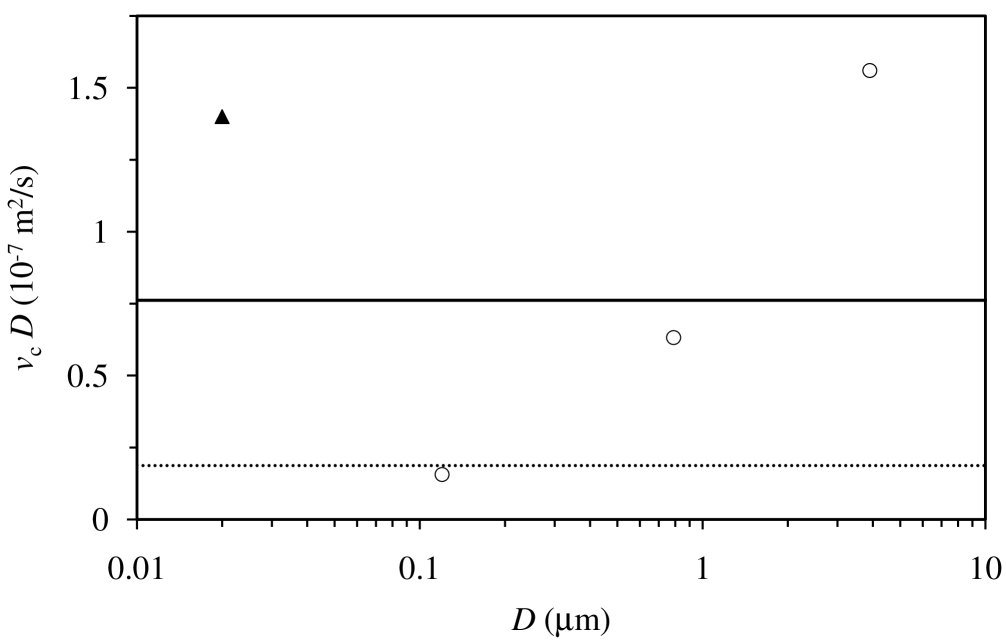
Figure 6: Critical velocity times the pore diameter for superfluid flow of helium through a cylindrical pore of diameter $D$. The circles (Pathria 1972 section 10.8) and triangle (Allum et al. 1977) are measured values, the solid line is the present prediction $v_{r}=2j_{01}\hbar/mD$, and the dotted line is the vortex result of Kawatra and Pathria (1966) $v_{\mathrm{c}}=1.18\hbar/mD$.

And third, there is momentum gap due to the size of the system; $\Delta_{p}=2\pi\hbar/L$ in rectangular geometry, and $\Delta_{p,\perp}=2j_{01}\hbar/D$ in cylindrical geometry (Blinder 2011), where $j_{01}=2.4$ is the first zero of the zeroth order Bessel function. This, combined with the second point, means that the critical velocity for superfluid flow is equal to the velocity of the first excited transverse state. Although it has previously been known that the critical velocity is on the order of $\hbar/mD$ (Fetter and Foot 2012), the present theory gives a quantitative value, a mathematical derivation, and a molecular justification for it (Attard 2021).

This predicted critical velocity is tested in Fig. 6. Over some three orders of magnitude in pore diameter it remains within a factor of three of the measured data. The Landau stability criterion for superfluid flow gives a critical velocity that is several orders of magnitude larger than the measured values (Batrouni et al. 2004). The vortex prediction of Kawatra and Pathria (1966), which implements Feynman’s (1954) suggestion that the rotons invented by Landau (1941) in his theory of superfluidity were in fact quantized vortices, is also compared in the figure. Although limited, the data in Fig. 6 lies closer to the present theory than the vortex/roton theory. More persuasive is Occam’s apothegm: of two explanations that equally describe the data, the simpler is to be preferred.

References

• Abramowitz M and Stegun IA 1970 Handbook of Mathematical Functions (Dover: New York)

• Allum DR McClintock PVE and Phillips A 1977 The breakdown of superfluidity in liquid He: an experimental test of Landau’s theory Phil. Trans. R. Soc. A 284 179

• Attard P 2018 Quantum Statistical Mechanics in Classical Phase Space. Expressions for the Multi-Particle Density, the Average Energy, and the Virial Pressure arXiv:1811.00730

• Attard P 2021 Quantum Statistical Mechanics in Classical Phase Space, (IOP Publishing: Bristol).

• Balibar S 2014 Superfluidity: how quantum mechanics became visible pages 93–117 in History of Artificial Cold, Scientific, Technological and Cultural Issues (Gavroglu K editor) (Dordrecht: Springer)

• Balibar S 2017 Laszlo Tisza and the two-fluid model of superfluidity C. R. Physique 18 586

• Batrouni GG, Ramstad T and Hansen A 2004 Free-energy landscape and the critical velocity of superfluid films Phil. Trans. R. Soc. Lond. A 362 1595

• Blinder SM 2011 Quantum-mechanical particle in a cylinder http://demonstrations.wolfram.com
  /QuantumMechanicalParticleInACylinder
  /WolframDemonstrationsProject

• Donnelly RJ 1995 The discovery of superfluidity Physics Today 48 30

• Donnelly RJ 2009 The two-fluid theory and second sound in liquid helium Physics Today 62 34

• Donnelly RJ and Barenghi CF 1998 The observed properties of liquid Helium at the saturated vapor pressure J. Phys. Chem. Ref. Data 27 1217

• Fetter AL and Foot CJ 2012 Bose Gas: Theory and Experiment, chapter 2 in Ultracold Bosonic and Fermionic Gases Edited by Levin K, Fetter AL, and Stamper-Kurn DM (Elsevier:Amsterdam)

• Feynman RP 1954 Atomic theory of the two-fluid model of liquid helium Phys. Rev. 94 262

• Kawatra MP and Pathria RK 1966 Quantized vortices in an imperfect Bose gas and the breakdown of superfluidity in liquid helium II Phys. Rev. 151 132

• Landau LD 1941 Two-fluid model of liquid helium II J. Phys. USSR 5 71. Also Phys. Rev. 60 356

• London F 1938 The $\lambda$-phenomenon of liquid helium and the Bose-Einstein degeneracy Nature 141 643

• Merzbacher E 1970 Quantum Mechanics 2nd edn (New York: Wiley)

• Messiah A 1961 Quantum Mechanics (Vol 1 and 2) (Amsterdam: North-Holland)

• Pathria RK 1972 Statistical Mechanics (Oxford: Pergamon Press)

• van Sciver SW 2012 Helium Cryogenics 2nd edn (New York: Springer)

• Tisza L 1938 Transport phenomena in helium II Nature 141 913

Appendix A Mixed Trimer

Following on from the mixed dimer of section IV.1, which is necessarily singly excited, here is analyzed the mixed trimer with one ground and two excited momentum state bosons,

$$\eta^{(1;2)}_{0*}({\bf q},{\bf p})=\sum_{j}^{N_{0}}\sum_{k,l}^{N_{*}}\!{}^{\prime}\;e^{-{\bf p}_{k}\cdot{\bf q}_{jl}/\mathrm{i}\hbar}e^{-{\bf p}_{l}\cdot{\bf q}_{lk}/\mathrm{i}\hbar}.$$ (A.1)

The summand is just a trimer chain, section IV.3. As for the dimer, this should be divided by $N_{0}$ to account for the fact that there are now $N_{0}-1$ ground momentum state bosons available for pure loops; with this prefactor we can leave $\eta_{0}=N_{0}!$ unchanged. The prime on the sum over excited bosons indicates that no two may be the same. But since the order matters each pair must be counted twice. There are $N_{0}N_{*}(N_{*}-1)$ such trimer loops, most of which will contribute nothing after averaging.

The canonical average, in the discrete momentum case is

$$\left\langle\eta^{(1;2)}_{0*}/N_{0}\right\rangle_{N_{0},N_{*},\mathrm{cl}}$$

$$= \frac{\Lambda^{3N_{*}}}{V^{N_{*}}}\prod_{j}^{N_{0}}\delta_{{\bf p}_{j},{\bf 0}}\prod_{k}^{N_{*}}\sum_{{\bf p}_{k}}\!^{(p_{k}>0)}e^{-\beta p_{k}^{2}/2m}$$

$$\mbox{ }\times\left\langle\frac{1}{N_{0}}\sum_{j}^{N_{0}}\sum_{k,l}^{N_{*}}\!{}^{\prime}e^{-{\bf p}_{k}\cdot{\bf q}_{jl}/\mathrm{i}\hbar}e^{-{\bf p}_{l}\cdot{\bf q}_{lk}/\mathrm{i}\hbar}\right\rangle_{N,\mathrm{cl}}$$

$$= \frac{\Lambda^{3N_{*}}}{V^{N_{*}}}\frac{N_{*}(N_{*}-1)}{N(N-1)(N-2)}$$

$$\mbox{ }\times\prod_{j}^{N_{0}}\delta_{{\bf p}_{j},{\bf 0}}\prod_{k}^{N_{*}}\sum_{{\bf p}_{k}}\!^{(p_{k}>0)}e^{-\beta p_{k}^{2}/2m}\int_{V}\mathrm{d}{\bf q}_{1}\,\mathrm{d}{\bf q}_{2}\,\mathrm{d}{\bf q}_{3}\;$$

$$\mbox{ }\times\rho^{(3)}_{N}({\bf q}_{1},{\bf q}_{2},{\bf q}_{3})e^{-{\bf p}_{1}\cdot{\bf q}_{12}/\mathrm{i}\hbar}e^{-{\bf p}_{2}\cdot{\bf q}_{23}/\mathrm{i}\hbar}.$$

In the final equality bosons 1 and 2 are in an excited momentum state and boson 3 is in the momentum ground state, although this makes no difference to the configuration integral.

The connected part of the triplet density is given by

$$\rho^{3}h^{(3)}_{N}({\bf q}_{1},{\bf q}_{2},{\bf q}_{3})$$ (A.3)

$$= \rho^{(3)}_{N}({\bf q}_{1},{\bf q}_{2},{\bf q}_{3})-\rho^{3}h^{(2)}_{N}(q_{12})-\rho^{3}h^{(2)}_{N}(q_{23})$$

$$\mbox{ }-\rho^{3}h^{(2)}_{N}(q_{31})-1.$$

This vanishes if any particle is taken far from the rest. Again we assume a homogeneous system.

The asymptotic contribution to the configurational integral is

$$\rho^{3}\int_{V}\mathrm{d}{\bf q}^{3}\;\left\{h^{(2)}_{N}(q_{12})+h^{(2)}_{N}(q_{23})+h^{(2)}_{N}(q_{31})+1\right\}$$ (A.4)

$$\mbox{ }\hskip 19.91684pt\times e^{-{\bf p}_{1}\cdot{\bf q}_{12}/\mathrm{i}\hbar}e^{-{\bf p}_{2}\cdot{\bf q}_{23}/\mathrm{i}\hbar}$$

$$= \rho^{3}V\delta_{{\bf p}_{2},{\bf 0}}\int_{V}\mathrm{d}{\bf q}_{12}\;h^{(2)}_{N}(q_{12})$$

$$\mbox{ }+\rho^{3}V\delta_{{\bf p}_{1},{\bf 0}}\int_{V}\mathrm{d}{\bf q}_{23}\;h^{(2)}_{N}(q_{23})$$

$$\mbox{ }+\rho^{3}V^{2}\delta_{{\bf p}_{1},{\bf p}_{2}}\int_{V}\mathrm{d}{\bf q}_{13}\;h^{(2)}_{N}(q_{31})e^{-{\bf p}_{1}\cdot{\bf q}_{13}/\mathrm{i}\hbar}$$

$$\mbox{ }+\rho^{3}V\delta_{{\bf p}_{1},{\bf 0}}\delta_{{\bf p}_{2},{\bf 0}}$$

$$= \rho^{3}V^{2}\delta_{{\bf p}_{1},{\bf p}_{2}}\int_{V}\mathrm{d}{\bf q}_{13}\;h^{(2)}_{N}(q_{31})e^{-{\bf p}_{1}\cdot{\bf q}_{13}/\mathrm{i}\hbar}.$$

Since $p_{1}>0$ and $p_{2}>0$, all the other terms vanish.

Separating out the surviving part of the asymptote one obtains

$$\left\langle\eta^{(1;2)}_{0*}/N_{0}\right\rangle_{N_{0},N_{*},\mathrm{cl}}$$ (A.5)

$$= \frac{\Lambda^{3N_{*}}}{V^{N_{*}}}\frac{N_{*}(N_{*}-1)}{N(N-1)(N-2)}\left\{\Delta_{p}^{-3N_{*}}\int\mathrm{d}{\bf p}^{N_{*}}\;e^{-\beta{\cal K}({\bf p}^{N_{*}})}\right.$$

$$\left.\mbox{ }\times\int\mathrm{d}{\bf q}^{3}\,\rho^{3}h^{(3)}_{N}({\bf q}_{1},{\bf q}_{2},{\bf q}_{3})e^{-{\bf p}_{1}\cdot{\bf q}_{12}/\mathrm{i}\hbar}e^{-{\bf p}_{2}\cdot{\bf q}_{23}/\mathrm{i}\hbar}\right.$$

$$\left.\mbox{ }+\Delta_{p}^{-3N_{*}}\int\mathrm{d}{\bf p}^{N_{*}}\;e^{-\beta{\cal K}({\bf p}^{N_{*}})}\delta_{{\bf p}_{1},{\bf p}_{2}}\right.$$

$$\left.\mbox{ }\times\rho^{3}V^{2}\int_{V}\mathrm{d}{\bf q}_{13}\;h^{(2)}_{N}(q_{31})e^{-{\bf p}_{1}\cdot{\bf q}_{13}/\mathrm{i}\hbar}\right\}$$

$$= \frac{N_{*}(N_{*}-1)}{N(N-1)(N-2)}\left\{\rho^{3}\int\mathrm{d}{\bf q}_{1}\,\mathrm{d}{\bf q}_{2}\,\mathrm{d}{\bf q}_{3}\,\right.$$

$$\left.\mbox{ }\times h^{(3)}_{N}({\bf q}_{1},{\bf q}_{2},{\bf q}_{3})e^{-\pi q_{12}^{2}/\Lambda^{2}}e^{-\pi q_{23}^{2}/\Lambda^{2}}\right.$$

$$\left.\mbox{ }+2^{-3/2}\rho^{3}V\Lambda^{3}\int_{V}\mathrm{d}{\bf q}_{13}\;h^{(2)}_{N}(q_{13})e^{-\pi q_{13}^{2}/2\Lambda^{2}}\right\}.$$

Both terms in the braces scale with volume and hence this mixed trimer term is intensive. The second term is likely negative, but the first integrand has positive contributions. This may be rewritten as classical canonical averages

$$\left\langle\eta^{(1;2)}_{0*}/N_{0}\right\rangle_{N_{0},N_{*},\mathrm{cl}}$$ (A.6)

$$= \frac{N_{*}^{2}}{N^{2}}\left\{\left<\frac{1}{N}\sum_{j,k,l}^{N}\!{}^{\prime}e^{-\pi q_{jk}^{2}/\Lambda^{2}}e^{-\pi q_{kl}^{2}/\Lambda^{2}}\right>_{N,\mathrm{cl}}\right.$$

$$\mbox{ }\left.-2\rho\Lambda^{3}\left<\frac{1}{N}\sum_{j,k}^{N}\!{}^{\prime}e^{-\pi q_{jk}^{2}/\Lambda^{2}}\right>_{N,\mathrm{cl}}+\rho^{2}\Lambda^{6}\right\}$$

$$= \frac{N_{*}^{2}}{N^{2}}\left<\frac{1}{N}\sum_{j,k,l}^{N}\!{}^{\prime}\left[e^{-\pi q_{jk}^{2}/\Lambda^{2}}-\frac{\rho\Lambda^{3}}{N}\right]\right.$$

$$\left.\mbox{ }\times\left[e^{-\pi q_{kl}^{2}/\Lambda^{2}}-\frac{\rho\Lambda^{3}}{N}\right]\right>_{N,\mathrm{cl}}$$

$$\equiv \frac{N_{*}^{2}}{N^{2}}\left\langle\tilde{\eta}^{(3)}/N\right\rangle_{N,\mathrm{cl}}^{\mathrm{corr}}.$$

Comparing the penultimate equality with Eq. (4.10), the general rule can be inferred.

As for the mixed dimer, section IV.1, one can replace the single ground state boson by the series of all the ground momentum state bosons, each of the $N_{0}$ terms of which have the same value, section IV.2. Their total contribution is

$$-\beta\Omega_{\mathrm{mix}}^{(2)} = \sum_{l=3}^{N_{0}+2}\left\langle\eta^{(l-2;2)}_{0*}/N_{0}\right\rangle_{N_{0},N_{*},\mathrm{cl}}$$ (A.7)

$$= N_{0}\left\langle\eta^{(1;2)}_{0*}/N_{0}\right\rangle_{N_{0},N_{*},\mathrm{cl}}$$

$$= \frac{N_{0}N_{*}^{2}}{N^{2}}\left\langle\tilde{\eta}^{(3)}/N\right\rangle_{N,\mathrm{cl}}^{\mathrm{corr}}.$$

The prefactor derivative changes sign at $N_{*}/N=2/3$.

Appendix B Corrigible Chains

The chain weights are corrected canonical averages,

$$\left\langle\tilde{\eta}\!^{(l)}/N_{0}\right\rangle_{N_{0},N_{*},\mathrm{cl}}=\frac{N_{*}^{l-1}}{N^{l-1}}\left\langle\tilde{\eta}\!^{(l)}/N\right\rangle_{N,\mathrm{cl}}^{\mathrm{corr}}.$$ (B.1)

Define the intensive uncorrected $l$-chain weight

$$\tilde{g}^{(l)}=\frac{1}{N}\left\langle\sum_{j_{1},\ldots,j_{l}}^{N}\!\!{}^{\prime}\;\prod_{k=1}^{l-1}e^{-\pi q_{j_{k},j_{k+1}}^{2}/\Lambda^{2}}\right\rangle_{N,\mathrm{cl}}.$$ (B.2)

The prime on the summation indicates that no two indeces may be the same.

This uncorrected chain weight is the simplest to implement computationally. Essentially this is because the head bosons come from the liquid volume, $N_{\mathrm{liq}}$, and this is different to the number of neighbors, ${\cal N}_{j_{1}}$, from which the tail of the chain is chosen. The uncorrected weight is intensive and is insensitive to ${\cal N}_{j_{1}}$.

The relations between the first several corrected and uncorrected chain weights are as follows. (Here $N=N_{\mathrm{liq}}$ and $\rho=N_{\mathrm{liq}}/V_{\mathrm{liq}}$. The product of the averages is used in the following expressions.) The dimer is

$$\left\langle\tilde{\eta}\!^{(2)}/N\right\rangle_{N,\mathrm{cl}}^{\mathrm{corr}} = \left\langle\frac{1}{N}\sum_{j,k}^{N}\!{}^{\prime}\left[e^{-\pi q_{jk}^{2}/\Lambda^{2}}-\frac{\rho\Lambda^{3}}{N}\right]\right\rangle_{N,\mathrm{cl}}$$ (B.3)

$$= \tilde{g}^{(2)}-\rho\Lambda^{3}.$$

The trimer is

$$\left\langle\tilde{\eta}\!^{(3)}/N\right\rangle_{N,\mathrm{cl}}^{\mathrm{corr}} = \left<\frac{1}{N}\sum_{j,k,l}^{N}\!{}^{\prime}\left[e^{-\pi q_{jk}^{2}/\Lambda^{2}}-\frac{\rho\Lambda^{3}}{N}\right]\right.$$ (B.4)

$$\left.\mbox{ }\times\left[e^{-\pi q_{kl}^{2}/\Lambda^{2}}-\frac{\rho\Lambda^{3}}{N}\right]\right>_{N,\mathrm{cl}}$$

$$= \tilde{g}^{(3)}-2\rho\Lambda^{3}\tilde{g}^{(2)}+(\rho\Lambda^{3})^{2}.$$

The tetramer is

$$\left\langle\tilde{\eta}\!^{(4)}/N\right\rangle_{N,\mathrm{cl}}^{\mathrm{corr}}$$

$$= \left<\frac{1}{N}\sum_{j,k,l,m}^{N}\!{}^{\prime}\left[e^{-\pi q_{jk}^{2}/\Lambda^{2}}-\frac{\rho\Lambda^{3}}{N}\right]\right.$$

$$\left.\mbox{ }\times\left[e^{-\pi q_{kl}^{2}/\Lambda^{2}}-\frac{\rho\Lambda^{3}}{N}\right]\left[e^{-\pi q_{lm}^{2}/\Lambda^{2}}-\frac{\rho\Lambda^{3}}{N}\right]\right>_{N,\mathrm{cl}}$$

$$= \tilde{g}^{(4)}-2\rho\Lambda^{3}\tilde{g}^{(3)}-\rho\Lambda^{3}\big{(}\tilde{g}^{(2)}\big{)}^{2}+3\rho^{2}\Lambda^{6}\tilde{g}^{(2)}-\rho^{3}\Lambda^{9}.$$

The pentamer is

$$\left\langle\tilde{\eta}\!^{(5)}/N\right\rangle_{N,\mathrm{cl}}^{\mathrm{corr}}$$ (B.6)

$$= \tilde{g}^{(5)}-2\rho\Lambda^{3}\tilde{g}^{(4)}-2\rho\Lambda^{3}\tilde{g}^{(3)}\tilde{g}^{(2)}+3(\rho\Lambda^{3})^{2}\tilde{g}^{(3)}$$

$$\mbox{ }+3(\rho\Lambda^{3})^{2}\big{(}\tilde{g}^{(2)}\big{)}^{2}-4(\rho\Lambda^{3})^{3}\tilde{g}^{(2)}+(\rho\Lambda^{3})^{4}.$$

The hexamer is

$$\left\langle\tilde{\eta}\!^{(6)}/N\right\rangle_{N,\mathrm{cl}}^{\mathrm{corr}}$$ (B.7)

$$= \tilde{g}^{(6)}-2\rho\Lambda^{3}\tilde{g}^{(5)}-2\rho\Lambda^{3}\tilde{g}^{(4)}\tilde{g}^{(2)}-\rho\Lambda^{3}\big{(}\tilde{g}^{(3)}\big{)}^{2}$$

$$\mbox{ }+2(\rho\Lambda^{3})^{2}\tilde{g}^{(4)}+7(\rho\Lambda^{3})^{2}\tilde{g}^{(3)}\tilde{g}^{(2)}+(\rho\Lambda^{3})^{2}\big{(}\tilde{g}^{(2)}\big{)}^{3}$$

$$\mbox{ }-4(\rho\Lambda^{3})^{3}\tilde{g}^{(3)}-6(\rho\Lambda^{3})^{3}\big{(}\tilde{g}^{(2)}\big{)}^{2}$$

$$\mbox{ }+5(\rho\Lambda^{3})^{4}\tilde{g}^{(2)}-(\rho\Lambda^{3})^{5}.$$

And the heptamer is

$$\left\langle\tilde{\eta}\!^{(7)}/N\right\rangle_{N,\mathrm{cl}}^{\mathrm{corr}}$$ (B.8)

$$= \tilde{g}^{(7)}-2\rho\Lambda^{3}\tilde{g}^{(6)}-2\rho\Lambda^{3}\tilde{g}^{(5)}\tilde{g}^{(2)}-2\rho\Lambda^{3}\tilde{g}^{(4)}\tilde{g}^{(3)}$$

$$\mbox{ }+3\rho^{2}\Lambda^{6}\tilde{g}^{(5)}+6\rho^{2}\Lambda^{6}\tilde{g}^{(4)}\tilde{g}^{(2)}+3\rho^{2}\Lambda^{6}\big{(}\tilde{g}^{(3)}\big{)}^{2}$$

$$\mbox{ }+3\rho^{2}\Lambda^{6}\tilde{g}^{(3)}\big{(}\tilde{g}^{(2)}\big{)}^{2}-4\rho^{3}\Lambda^{9}\tilde{g}^{(4)}-12\rho^{3}\Lambda^{9}\tilde{g}^{(3)}\tilde{g}^{(2)}$$

$$\mbox{ }-4\rho^{3}\Lambda^{9}\big{(}\tilde{g}^{(2)}\big{)}^{3}+5\rho^{4}\Lambda^{12}\tilde{g}^{(3)}+10\rho^{4}\Lambda^{12}\big{(}\tilde{g}^{(2)}\big{)}^{2}$$

$$\mbox{ }-6\rho^{5}\Lambda^{15}\tilde{g}^{(2)}+\rho^{6}\Lambda^{18}.$$

A useful check on these is that the magnitude of the coefficients must add to $2^{l-1}$. These results for $l\geq 4$ rely upon the inferred form for the corrected average.