Local Lagrangian reduced-order modeling for Rayleigh–Taylor instability by solution manifold decomposition

Abstract

Rayleigh–Taylor instability is a classical hydrodynamic instability of great interest in various disciplines of science and engineering, including astrophyics, atmospheric sciences and climate, geophysics, and fusion energy. Analytical methods cannot be applied to explain the long-time behavior of Rayleigh–Taylor instability, and therefore numerical simulation of the full problem is required. However, in order to capture the growth of amplitude of perturbations accurately, both the spatial and temporal discretization need to be extremely fine for traditional numerical methods, and the long-time simulation may become prohibitively expensive. In this paper, we propose efficient reduced order model techniques to accelerate the simulation of Rayleigh–Taylor instability in compressible gas dynamics. We introduce a general framework for decomposing the solution manifold to construct the temporal domain partition and temporally-local reduced order model construction with varying Atwood number. We propose two practical approaches in this framework, namely decomposition by using physical time and by penetration distance respectively. Numerical results are presented to examine the performance of the proposed approaches.

1 Introduction

Rayleigh–Taylor instability is a classical hydrodynamic instability occuring at the interface between two fluids of different densities. A denser fluid is initially supported on top by a less dense fluid with a counterbalancing pressure gradient under the effects of a gravitational field. It was first introduced by Rayleigh [1] in 1882 and further investigated by Taylor [2]. In recent years, it has been applied to various disciplines of science and engineering, including astrophyics [3, 4, 5, 6], atmospheric sciences and climate [7, 8], geophysics [9, 10, 11], and fusion energy [12, 13]. The readers are referred to [14, 15, 16] for a comprehensive overview of Rayleigh–Taylor instability.

In recent years, numerous research efforts have been devoted to modeling the growth of Rayleigh–Taylor instability mathematically and numerically, so as to provide better understanding of the nonlinear dynamics. Linear stability theory can be used to analytically derive the exponential growth in the amplitude in the subwavelength regime in the short-time dynamics [2]. However, as the nonlinearity dominates and the dynamics become chaotic in the later stages, numerical simulation plays an important role in the studies of the long-time dynamics [17, 18, 19, 20, 21]. Depending on the nature of the fluids, the physical process is governed by a set of conservation laws and mathematically modeled by a system of partial differential equations. In this work, we consider the scenario of a single-mode two-dimensional Rayleigh–Taylor instability between two compressible and isotropic ideal gases with different densities, in a parametric setting. The Euler equation is used to model the compressible gas dynamics in a complex multimaterial setting. Moreover, we study the effects of Atwood number as a problem parameter on the physical quantities. The governing equations are numerically solved in a moving Lagrangian frame, where the computational mesh is moved along with the fluid velocity. Our work is built on [22], where a general framework of high-order curvilinear finite elements and adaptive time stepping of explicit time integrators is proposed for numerical discretization of the Lagrangian hydrodynamics problem over general unstructured two-dimensional and three-dimensional computational domains. The method shows great capability and lots of advantages, including high-order accuracy, total energy conservation, and the Rankine-Hugoniot jump conditions fulfilled at shock boundaries. However, forward simulations of Lagrangian hydrodynamics can be computationally very expensive, especially in long-time simulation of highly nonlinear problems like Rayleigh–Taylor instability. It is therefore desirable to develop efficient techniques for accelerating the computationally expensive simulations. In this work, we propose new reduced order model (ROM) techniques for Rayleigh–Taylor instability in compressible Euler equations.

A reduced order model has nowadays become a popular and actively researched computational technique to reduce the computational cost of simulations while minimizing the error introduced in the reduction process. Many physics-based models are complex and nonlinear, and are formulated on large spatio-temporal domains, in which the computational cost can be prohibitively high. It may take a long time to run one forward simulation even with high performance computing. In decision-making applications where multiple forward simulations are needed, such as parameter study, design optimization [23, 24, 25, 26], optimal control [27, 28], uncertainty quantification [29, 30], and inverse problems [31, 30], the computationally expensive simulations are not desirable. To this end, a reduced order model can be useful to obtain sufficiently accurate approximate solutions with considerable speed-up compared to a corresponding full order model (FOM).

Many model reduction schemes have been developed to reduce the computational cost of simulations while minimizing the error introduced in the reduction process. Most of these approaches seek to extract an intrinsic solution subspace for condensed solution representation by a linear combination of reduced basis vectors. The reduced basis vectors are extracted from performing proper orthogonal decomposition (POD) on the snapshot data of the FOM simulations. The number of degrees of freedom is then reduced by substituting the ROM solution representation into the (semi-)discretized governing equation. These approaches take advantage of both the known governing equation and the solution data generated from the corresponding FOM simulations to form linear subspace reduced order models (LS-ROM). Example applications include, but are not limited to, the nonlinear diffusion equations [32, 33], the Burgers equation and the Euler equations in small-scale [34, 35, 36], the convection–diffusion equations [37, 38], the Navier–Stokes equations [39, 40], rocket nozzle shape design [41], flutter avoidance wing shape optimization [42], topology optimization of wind turbine blades [43], lattice structure design [44], porous media flow/reservoir simulations [45, 46, 47, 48], computational electro-cardiology [49], inverse problems [50], shallow water equations [51, 52], Boltzmann transport problems [53], computing electromyography [54], spatio-temporal dynamics of a predator–prey system [55], acoustic wave-driven microfluidic biochips [56], and Schrödinger equation [57]. Survey papers for the projection-based LS-ROM techniques can be found in [58, 59].

In spite of successes of the classical LS-ROM in many applications, these approaches are limited to the assumption that the intrinsic solution space falls into a subspace with a small dimension, i.e., the solution space with a Kolmogorov $n$-width decaying fast. This assumption is violated in advection-dominated problems, due to features such as sharp gradients, moving shock fronts, and turbulence, which hinder these model reduction schemes from being practical. Our goal in this paper is to develop an efficient reduced order model for hydrodynamics simulation with advection-dominated solutions. Some reduced order model techniques for hydrodynamics or turbulence models in the literature include [60, 61, 62, 63, 64, 65, 66], which are mostly built on the Eulerian formulation, i.e., the computational mesh is stationary with respect to the fluid motion. In contrast, numerical methods in the Lagrangian formulation, which are characterized by a computational mesh that moves along with the fluid velocity, are developed for better capturing the shocks and preserving the conserved quantities in advection-dominated problems. It therefore becomes natural to develop Lagrangian-based reduced order models to overcome the challenges posed by advection-dominated problems. Some existing work in this research direction include [37, 67], where a Lagrangian POD and dynamic mode decomposition (DMD) reduced order model are introduced respectively for the one-dimensional nonlinear advection-diffusion equation. We remark that there are some similarities and differences between our work and [37] in using POD for developing Lagrangian-based reduced order models. It is important to note that our work is based on the more complicated and challenging two-dimensional compressible Euler equations. The reduced bases are built independently for each state variable in our work, while a single basis is built for the whole state in [37]. Furthermore, we introduce the solution manifold decomposition concept so as to ensure adequate ROM speed-up by classifying solution snapshot samples for constructing ROM spaces with low dimension and assigning the appropriate ROM to be used in the time marching.

Recently, there have been many attempts to develop efficient ROMs for the advection-dominated or sharp gradient problems. The attempts can be divided mainly into two categories. The first category enhances the solution representability of the linear subspace by introducing some special treatments and adaptive schemes. A dictionary-based model reduction method for the approximation of nonlinear hyperbolic equations is developed in [68], where the reduced approximation is obtained from the minimization of the residual in the $L_{1}$ norm for the reduced linear subspace. In [69], a fail-safe $h$-adaptive algorithm is developed. The algorithm enables ROMs to be incrementally refined to capture the shock phenomena which are unobserved in the original reduced basis through a-posteriori online enrichment of the reduced-basis space by decomposing a given basis vector into several vectors with disjoint support. The windowed least-squares Petrov–Galerkin model reduction for dynamical systems with implicit time integrators is introduced in [70, 71], which can overcome the challenges arising from the advection-dominated problems by representing only a small time window with a local ROM. Our previous work [72] adopts a similar approach for Lagrangian hydrodynamics. Another active research direction is to exploit the sharp gradients and represent spatially local features in ROM, such as the online adaptivity bases and adaptive sampling approach [73] and the shock reconstruction surrogate approach [74]. In [75], an adaptive space-time registration-based model reduction is used to align local features of parameterized hyperbolic PDEs in a fixed one-dimensional reference domain. Some new approaches have been developed for aligning the sharp gradients by using a superposition of snapshots with shifts or transforms. In [76], the shifted proper orthogonal decomposition (sPOD) introduces time-dependent shifts of the snapshot matrix in POD in an attempt to separate different transport velocities in advection-dominated problems. The practicality of this approach relies heavily on accurate determination of shifted velocities. In [77], an iterative transport reversal algorithm is proposed to decompose the snapshot matrix into multiple shifting profiles. In [78], inspired by the template fitting [79], a high resolution transformed snapshot interpolation with an appropriate behavior near singularities is considered.

The second category replaces the linear subspace solution representation with the nonlinear manifold, which is a very active research direction. Recently, a neural network-based reduced order model is developed in [80] and extended to preserve the conserved quantities in the physical conservation laws [81]. In these approaches, the weights and biases in the neural network are determined in the training phase, and existing numerical methods, such as finite difference and finite element methods, are utilized. However, since the nonlinear terms need to be updated every time step or Newton step, and the computation of the nonlinear terms still scale with the FOM size, these approaches do not achieve any speed-up with respect to the corresponding FOM. Recently, Kim, et al., have achieved a considerable speed-up with the nonlinear manifold reduced order model [82, 83], but it was only applied to small problems. Manifold approximations via transported subspaces in [84] introduced a low-rank approximation to the transport dynamics by approximating the solution manifold with a transported subspace generated by low-rank transport modes. However, their approach is limited to a one-dimensional problem setting. In [85], a depth separation approach for reduced deep networks in nonlinear model reduction is presented, in which the reduced order model is composed with hidden layers with low-rank representation.

The method presented in this paper belongs to the first category. The underlying concept is to build small and accurate projection-based reduced-order models by decomposing the solution manifold into submanifolds. These reduced-order models are local in the sense that each of them will be valid only over a certain sub-interval of the temporal domain. The appropriate local reduced order model is chosen based on the current state of the system, and all the local reduced order models will cover the whole time marching in the online phase. The concept of a local reduced order model was introduced in [86, 87], where unsupervised clustering is used for the solution manifold decomposition. In our work, the solution manifold decomposition is based on a suitably defined physics-based indicator, which generalizes the time-windowing ROM approach for Lagrangian hydrodynamics simulations in our previous work [72]. The idea of time-windowing ROM is to construct temporally-local ROM spaces which are small but accurate within a short period in advection-dominated problems. The method provided tremendous speed-up and accurate approximated solutions in various benchmark experiments including Sedov blast, Gresho vortices, Taylor-Green vortices, and triple-point problems. However, in order to approximate the solutions of Rayleigh–Taylor instability over a range of Atwood number, the time-windowing approach is insufficient to provide good approximations, since the penetration speed of the fluid interface varies with the Atwood number. In this work, we modify our ROM approach by introducing new techniques to capture the fast-moving shock boundaries, which provide significant improvements in Rayleigh–Taylor instability.

Our contribution in this paper is to propose an efficient model order reduction scheme for accelerating the simulation of Rayleigh–Taylor instability in compressible gas dynamics with varying Atwood number. Similar to [72], the idea is to construct temporally-local ROM spaces which are small but accurate within a short period in advection-dominated problems to achieve a good speed-up and solution accuracy. Proper orthogonal decomposition (POD) is used to extract the dominant modes in solution representability, the solution nonlinear subspace (SNS) method is used to establish the subspace relations and construct the nonlinear term bases as in [35], and an oversampling discrete empirical interpolation method (DEIM) serves as a hyper-reduction technique to reduce the complexity due to the nonlinear terms in the governing equations. The difference between this work and [72] is the introduction of a new temporal domain partition scheme that allows a smaller dimension of reduced basis in each temporal subdomain and use of temporally-local ROMs at different Atwood numbers for better solution accuracy. In this work, we propose a general framework to decompose the solution manifold by a suitably defined indicator. The indicator is used to classify solution snapshot samples for constructing ROM spaces with low dimension and to assign the appropriate ROM to be used in the time marching. We consider two such indicators, namely the physical time and the penetration distance, and compare the performance in speed-up and solution accuracy. As we will see in our numerical experiments, the penetration distance is a good alternative indicator to resolve the deficiency of degenerating solution accuracy with respect to Atwood number observed in the time-windowing approach. We remark that, by taking the advantage of Lagrangian formulation of the Euler equations, the penetration distance is easily accessible and plays an important role in the newly proposed distance-windowing approach.

The rest of the paper is organized as follows. In Section 2, we introduce the governing equations and the numerical discretization which will be used as the full order model. Next, a projection-based ROM is described in Section 3. In Section 4, a general framework of solution manifold decomposition is introduced, and two practical examples will be discussed. Numerical results are presented in Section 5. Finally, conclusions are given in Section 6.

2 Numerical modeling

In this section, we describe a direct numerical simulation methodology for Rayleigh–Taylor instability in compressible gas dynamics, using a finite element method, which will serve as the full order model in this work. We first present the governing equations, initial and boundary conditions which give rise to Rayleigh–Taylor instability. We also present the key ingredients of the numerical solver.

2.1 Governing equations

We consider the two-dimensional mathematical model of Rayleigh–Taylor hydrodynamic instability caused by a gravitational field acting on compressible isotropic ideal gas with stratified densities. Suppose $t_{f}>0$ is the final time of the hydrodynamic process. For $t\in[0,t_{f}]$, let $\Omega(t)\subset\mathbb{R}^{2}$ denote a continuous medium which deforms in time, with the initial configuration at $t=0$ being a rectangular domain $\widetilde{\Omega}=\Omega(0)=[0,1/2]\times[-1,1]$ with aspect ratio 1:4. The compressible gas dynamics is modeled by the Euler equations in a Lagrangian reference frame [88], driven by a constant gravitational acceleration $g$:

(2.1) $$\text{momentum conservation}: \rho\frac{dv}{dt} =\nabla\cdot\sigma+g$$

$$\text{mass conservation}: \dfrac{1}{\rho}\frac{d\rho}{dt} =-\nabla\cdot v$$

$$\text{energy conservation}: \rho\frac{de}{dt} =\sigma:\nabla v$$

$$\text{equation of motion}: \frac{dx}{dt} =v.$$

Here, $\frac{d}{dt}=\frac{\partial}{\partial t}+v\cdot\nabla$ is the material derivative, $\rho$ denotes the density of the fluid, $\sigma$ denotes the deformation stress tensor, $x$ denotes the Lagrangian position, $v$ denotes the velocity, and $e$ denotes the internal energy per unit mass. Each of these physical quantities depends on the time $t\in[0,t_{f}]$ and the Eulerian coordinates of the particle $\widetilde{x}\in\widetilde{\Omega}$. In gas dynamics, the stress tensor is isotropic, and we write $\sigma=-pI+\sigma_{a}$, where $p$ denotes the thermodynamic pressure, and $\sigma_{a}$ denotes the artificial viscosity stress. Due to the ideal gas assumption, the thermodynamic pressure is related to the density and the internal energy by the equation of state

(2.2) $$p=(\gamma-1)\rho e,$$

where the adiabatic index is $\gamma=5/3$. For $t>0$, the system is prescribed with a boundary condition $v\cdot n=0$, where $n$ is the outward normal unit vector on the domain boundary. In order to close the system, an initial condition needs to be imposed. We assume the gas is initially stratified at the interface $\widetilde{x}_{2}=0$, supported by a counterbalancing pressure gradient and perturbed by a velocity. In mathematical terms, at the time $t=0$, for $\widetilde{x}=(\widetilde{x}_{1},\widetilde{x}_{2})\in\widetilde{\Omega}$, we take

(2.3) $$\begin{split}v(0,\widetilde{x})&=\left(0,0.02\cos(2\pi\widetilde{x}_{1})\exp(-2\pi\widetilde{x}_{2}^{2})\right)\\ \rho(0,\widetilde{x})&=\begin{cases}R&\text{ if }\widetilde{x}_{2}\geq 0\\ 1&\text{ if }\widetilde{x}_{2}<0\end{cases}\\ e(0,\widetilde{x})&=\dfrac{4+R-\rho\widetilde{x}_{2}}{(\gamma-1)\rho},\end{split}$$

where $R>1$ is the density ratio of the fluids. In the context of hydrodynamic instability, we define the dimensionless Atwood number by

(2.4) $$A=\dfrac{R-1}{R+1},$$

which increases mildly with the density ratio $R$. The density ratio and the Atwood number play an important role in the perturbation of the fluid interface. In our work, the mathematical model is considered in the parametric setting by regarding the Atwood number $A$ as a problem parameter which lies in a parametric domain $\mathsf{D}\subset\mathbb{R}$. In this way, the physical quantities are treated as functions not only of the time $t\in[0,t_{f}]$ and the Eulerian coordinates of the particle $\widetilde{x}\in\widetilde{\Omega}$, but also the problem parameter $A\in\mathsf{D}$.

2.2 Finite element modeling

In [22], a general framework of high-order curvilinear finite elements and adaptive time stepping of explicit time integrators is proposed for numerical discretization of the Lagrangian hydrodynamics problem over general unstructured two-dimensional and three-dimensional computational domains. Using general high-order polynomial basis functions for approximating the state variables, and curvilinear meshes for capturing the geometry of the flow and maintaining robustness with respect to mesh motion, the method achieves high-order accuracy. On the other hand, a modification is made to the second-order Runge-Kutta method to compensate for the lack of total energy conservation in standard high-order time integration techniques. The introduction of an artificial viscosity tensor further generates the appropriate entropy and ensures the Rankine-Hugoniot jump conditions at shock boundaries.

Following [22], we adopt a spatial discretization for (2.1) using a kinematic space $\mathcal{V}\subset[H^{1}(\widetilde{\Omega})]^{d}$ for approximating the position and the velocity, and a thermodynamic space $\mathcal{E}\subset L_{2}(\widetilde{\Omega})$ for approximating the energy. The density can be eliminated, and the equation of mass conservation can be decoupled from (2.1). We assume high-order finite element (FE) discretization in space, and the finite dimensions $N_{\mathcal{V}}$ and $N_{\mathcal{E}}$ are the global numbers of FE degrees of freedom in the corresponding discrete FE spaces. For more details, see [22]. The FE coefficient vector functions for velocity and position are denoted as $\boldsymbol{v},\boldsymbol{x}:[0,t_{f}]\times\mathsf{D}\rightarrow\mathbb{R}^{N_{\mathcal{V}}}$, and the coefficient vector function for energy is denoted as $\boldsymbol{e}:[0,t_{f}]\times\mathsf{D}\rightarrow\mathbb{R}^{N_{\mathcal{E}}}$. The semidiscrete Lagrangian conservation laws can be expressed as a nonlinear system of differential equations in the coefficients with respect to the bases for the kinematic and thermodynamic spaces:

(2.5) $$\text{momentum conservation}: \boldsymbol{M}_{\mathcal{V}}\frac{d\boldsymbol{v}}{dt} =-\boldsymbol{F}(\boldsymbol{v},\boldsymbol{e},\boldsymbol{x};A)\cdot\boldsymbol{1}+\boldsymbol{M}_{\mathcal{V}}\mathbf{g}$$

$$\text{energy conservation}: \boldsymbol{M}_{\mathcal{E}}\frac{d\boldsymbol{e}}{dt} =\boldsymbol{F}(\boldsymbol{v},\boldsymbol{e},\boldsymbol{x};A)^{T}\cdot\boldsymbol{v}$$

$$\text{equation of motion}: \frac{d\boldsymbol{x}}{dt} =\boldsymbol{v},$$

where $\boldsymbol{M}_{\mathcal{V}}\mathbf{g}$ denotes the effects of the gravitation force in the discrete system.

Let $\boldsymbol{y}\equiv(\boldsymbol{v};\boldsymbol{e};\boldsymbol{x})^{T}\in\mathbb{R}^{N}$, $N=2N_{\mathcal{V}}+N_{\mathcal{E}}$, be the hydrodynamic state vector. Then the semidiscrete conservation equation of (2.5) can be written in a compact form as

(2.6) $$\frac{d\boldsymbol{y}}{dt}=\mathsf{F}(\boldsymbol{y};A),$$

where the nonlinear force term, $\mathsf{F}:\mathbb{R}^{N}\times\mathsf{D}\rightarrow\mathbb{R}^{N}$, is defined as

(2.7) $$\mathsf{F}(\boldsymbol{y};A) \equiv\begin{pmatrix}\mathsf{F}_{v}(\boldsymbol{v},\boldsymbol{e},\boldsymbol{x};A)\\ \mathsf{F}_{e}(\boldsymbol{v},\boldsymbol{e},\boldsymbol{x};A)\\ \mathsf{F}_{x}(\boldsymbol{v},\boldsymbol{e},\boldsymbol{x};A)\end{pmatrix}\equiv\begin{pmatrix}-\boldsymbol{M}_{\mathcal{V}}^{-1}\mathsf{F}^{\mathfrak{1}}(\boldsymbol{y};A)+\mathbf{g}\\ \boldsymbol{M}_{\mathcal{E}}^{-1}\mathsf{F}^{tv}(\boldsymbol{y};A)\\ \boldsymbol{v}\end{pmatrix},$$

where $\mathsf{F}^{\mathfrak{1}}:\mathbb{R}^{N}\times\mathsf{D}\rightarrow\mathbb{R}^{N_{\mathcal{V}}}$ and $\mathsf{F}^{tv}:\mathbb{R}^{N}\times\mathsf{D}\rightarrow\mathbb{R}^{N_{\mathcal{E}}}$ are nonlinear vector functions that are defined respectively as

(2.8) $$\mathsf{F}^{\mathfrak{1}}(\boldsymbol{y};A) \equiv\boldsymbol{F}(\boldsymbol{v},\boldsymbol{e},\boldsymbol{x};A)\cdot\boldsymbol{1}, \mathsf{F}^{tv}(\boldsymbol{y};A) \equiv\boldsymbol{F}(\boldsymbol{v},\boldsymbol{e},\boldsymbol{x};A)^{T}\cdot\boldsymbol{v}.$$

From now on, we drop the dependence on the parameter $A$ to simplify the notations where there is no ambiguity.

In order to obtain a fully discretized system of equations, one needs to apply a time integrator. We consider an explicit Runge-Kutta scheme called the RK2-average scheme, which is proved to conserve the discrete total energy exactly (see Proposition 7.1 of [22]). The temporal domain is discretized as $\{t_{n}\}_{n=0}^{N_{t}}$, where $t_{n}$ denotes a discrete moment in time with $t_{0}=0$, $t_{N_{t}}=t_{f}$, and $t_{n-1}<t_{n}$ for $n\in{\rm Nature}{N_{t}}$, where ${\rm Nature}{N}\equiv\{1,\ldots,N\}$. The computational domain at time $t_{n}$ is denoted as $\Omega^{n}\equiv\Omega(t_{n})$. We denote the quantities of interest defined on $\Omega^{n}$ with a subscript $n$. Starting with $\boldsymbol{v}_{0}=\boldsymbol{v}(0)$, $\boldsymbol{e}_{0}=\boldsymbol{e}(0)$, and $\boldsymbol{x}_{0}=\boldsymbol{x}(0)$, the discrete state is updated by

(2.9) $$\boldsymbol{v}_{n+\frac{1}{2}} =\boldsymbol{v}_{n}+(\Delta t_{n}/2)(-\boldsymbol{M}_{\mathcal{V}}^{-1}\mathsf{F}^{\mathfrak{1}}_{n}+\mathbf{g}), \boldsymbol{v}_{n+1} =\boldsymbol{v}_{n}+\Delta t_{n}(-\boldsymbol{M}_{\mathcal{V}}^{-1}\mathsf{F}^{\mathfrak{1}}_{n+\frac{1}{2}}+\mathbf{g}),$$

(2.10) $$\boldsymbol{e}_{n+\frac{1}{2}} =\boldsymbol{e}_{n}+(\Delta t_{n}/2)\boldsymbol{M}_{\mathcal{E}}^{-1}\mathsf{F}^{tv}_{n}, \boldsymbol{e}_{n+1} =\boldsymbol{e}_{n}+\Delta t_{n}\boldsymbol{M}_{\mathcal{E}}^{-1}\bar{\mathsf{F}}^{tv}_{n+\frac{1}{2}},$$

(2.11) $$\boldsymbol{x}_{n+\frac{1}{2}} =\boldsymbol{x}_{n}+(\Delta t_{n}/2)\boldsymbol{v}_{n+\frac{1}{2}}, \boldsymbol{x}_{n+1} =\boldsymbol{x}_{n}+\Delta t_{n}\bar{\boldsymbol{v}}_{n+\frac{1}{2}},$$

where the state $\boldsymbol{y}_{n}=(\boldsymbol{v}_{n};\boldsymbol{e}_{n};\boldsymbol{x}_{n})^{T}\in\mathbb{R}^{N}$ is used to compute the updates

(2.12) $$\mathsf{F}^{\mathfrak{1}}_{n} =\left(\boldsymbol{F}(\boldsymbol{y}_{n})\right)\cdot\boldsymbol{1}, \mathsf{F}^{tv}_{n} =\left(\boldsymbol{F}(\boldsymbol{y}_{n})\right)^{T}\cdot\boldsymbol{v}_{n+\frac{1}{2}},$$

in the first stage. Similarly, $\boldsymbol{y}_{n+\frac{1}{2}}=(\boldsymbol{v}_{n+\frac{1}{2}};\boldsymbol{e}_{n+\frac{1}{2}};\boldsymbol{x}_{n+\frac{1}{2}})^{T}\in\mathbb{R}^{N}$ is used to compute the updates

(2.13) $$\mathsf{F}^{\mathfrak{1}}_{n+\frac{1}{2}} =\left(\boldsymbol{F}(\boldsymbol{y}_{n+\frac{1}{2}})\right)\cdot\boldsymbol{1}, \bar{\mathsf{F}}^{tv}_{n+\frac{1}{2}} =\left(\boldsymbol{F}(\boldsymbol{y}_{n+\frac{1}{2}})\right)^{T}\cdot\bar{\boldsymbol{v}}_{n+\frac{1}{2}},$$

with $\bar{\boldsymbol{v}}_{n+\frac{1}{2}}=(\boldsymbol{v}_{n}+\boldsymbol{v}_{n+1})/2$ in the second stage. Note that the RK2-average scheme is different from the midpoint RK2 scheme in the updates for energy and position. The RK2-average scheme uses the midpoint velocity $\boldsymbol{v}_{n+\frac{1}{2}}$ and the average velocity $\bar{\boldsymbol{v}}_{n+\frac{1}{2}}$ to update energy and position in the first stage and the second stage respectively, while the midpoint RK2 uses the initial velocity $\boldsymbol{v}_{n}$ and the midpoint velocity $\boldsymbol{v}_{n+\frac{1}{2}}$. Since an explicit Runge-Kutta method is used, we need to control the time step size in order to maintain the stability of the fully discrete scheme. We follow the automatic time step control algorithm described in Section 7.3 of [22], where the time step size is controlled by estimates at all quadrature points in the mesh used in the evaluation of the force matrix $\boldsymbol{F}$.

3 Reduced order model

In this section, we present the details of the projection-based reduced oder model for the semi-discrete Lagrangian conservation laws (2.5). The reduced order model is constructed in the offline phase and deployed in the online phase. In what follows, we first discuss all the essential ingredients of the reduced order model, and move on to discuss the construction.

3.1 ROM simulation

In the reduced order model, we restrict our solution space to a subspace spanned by a reduced basis for each field. That is, the subspaces for velocity, energy, and position fields are defined as

(3.1) $$\mathcal{S}_{v} \equiv\text{Span}\{\mathbf{\phi}_{v}^{i}\}_{i=1}^{n_{v}}\subseteq\mathbb{R}^{N_{\mathcal{V}}}, \mathcal{S}_{e} \equiv\text{Span}\{\mathbf{\phi}_{e}^{i}\}_{i=1}^{n_{e}}\subseteq\mathbb{R}^{N_{\mathcal{E}}}, \mathcal{S}_{x} \equiv\text{Span}\{\mathbf{\phi}_{x}^{i}\}_{i=1}^{n_{x}}\subseteq\mathbb{R}^{N_{\mathcal{V}}},$$

with $\dim(\mathcal{S}_{v})=n_{v}\ll N_{\mathcal{V}}$, $\dim(\mathcal{S}_{e})=n_{e}\ll N_{\mathcal{E}}$, and $\dim(\mathcal{S}_{x})=n_{x}\ll N_{\mathcal{V}}$. Using these subspaces, each discrete field is approximated in trial subspaces, $\boldsymbol{v}\approx\tilde{\boldsymbol{v}}\in\boldsymbol{v}_{\text{os}}+\mathcal{S}_{v}$, $\boldsymbol{e}\approx\tilde{\boldsymbol{e}}\in\boldsymbol{e}_{\text{os}}+\mathcal{S}_{e}$, and $\boldsymbol{x}\approx\tilde{\boldsymbol{x}}\in\boldsymbol{x}_{\text{os}}+\mathcal{S}_{x}$. For a generic problem parameter $A\in\mathsf{D}$, we write

(3.2) $$\tilde{\boldsymbol{v}}(t;A) =\boldsymbol{v}_{\text{os}}(A)+\mathbf{\Phi}_{v}\widehat{\boldsymbol{v}}(t;A),$$

(3.3) $$\tilde{\boldsymbol{e}}(t;A) =\boldsymbol{e}_{\text{os}}(A)+\mathbf{\Phi}_{e}\widehat{\boldsymbol{e}}(t;A),$$

(3.4) $$\tilde{\boldsymbol{x}}(t;A) =\boldsymbol{x}_{\text{os}}(A)+\mathbf{\Phi}_{x}\widehat{\boldsymbol{x}}(t;A),$$

where $\boldsymbol{v}_{\text{os}}(A)\in\mathbb{R}^{N_{\mathcal{V}}}$, $\boldsymbol{e}_{\text{os}}(A)\in\mathbb{R}^{N_{\mathcal{E}}}$, and $\boldsymbol{x}_{\text{os}}(A)\in\mathbb{R}^{N_{\mathcal{V}}}$ denote the prescribed offset vectors for velocity, energy, and position fields respectively; the orthonormal basis matrices $\mathbf{\Phi}_{v}\in\mathbb{R}^{N_{\mathcal{V}}\times n_{v}}$, $\mathbf{\Phi}_{e}\in\mathbb{R}^{N_{\mathcal{E}}\times n_{e}}$, and $\mathbf{\Phi}_{x}\in\mathbb{R}^{N_{\mathcal{V}}\times n_{x}}$ are defined as

(3.5) $$\mathbf{\Phi}_{v} \equiv\begin{bmatrix}\mathbf{\phi}_{v}^{1}&\cdots&\mathbf{\phi}_{v}^{n_{v}}\end{bmatrix}, \mathbf{\Phi}_{e} \equiv\begin{bmatrix}\mathbf{\phi}_{e}^{1}&\cdots&\mathbf{\phi}_{e}^{n_{e}}\end{bmatrix}, \mathbf{\Phi}_{x} \equiv\begin{bmatrix}\mathbf{\phi}_{x}^{1}&\cdots&\mathbf{\phi}_{x}^{n_{x}}\end{bmatrix};$$

and $\widehat{\boldsymbol{v}}:[0,t_{f}]\times\mathsf{D}\rightarrow\mathbb{R}^{n_{v}}$, $\widehat{\boldsymbol{e}}:[0,t_{f}]\times\mathsf{D}\rightarrow\mathbb{R}^{n_{e}}$, and $\widehat{\boldsymbol{x}}:[0,t_{f}]\times\mathsf{D}\rightarrow\mathbb{R}^{n_{x}}$ denote the time-dependent generalized coordinates for velocity, energy, and position fields, respectively. One natural choice of the offset vectors is to use the initial values, i.e. $\boldsymbol{v}_{\text{os}}(A)=\boldsymbol{v}(0;A)$, $\boldsymbol{e}_{\text{os}}(A)=\boldsymbol{e}(0;A)$, and $\boldsymbol{x}_{\text{os}}(A)=\boldsymbol{x}(0;A)$.

The nonlinear matrix function, $\boldsymbol{F}$, changes every time the state variables evolve. Additionally, it needs to be multiplied by the basis matrices whenever updates in the nonlinear term occur, which scales with the FOM size. Therefore, we cannot expect any speed-up without special treatment of the nonlinear terms. To overcome this issue, a hyper-reduction technique needs to be applied (cf. [89]), where $\mathsf{F}^{\mathfrak{1}}$ and $\mathsf{F}^{tv}$ are approximated as

(3.6) $$\mathsf{F}^{\mathfrak{1}} \approx\mathbf{\Phi}_{\mathsf{F}^{\mathfrak{1}}}\widehat{\mathsf{F}^{\mathfrak{1}}}, \mathsf{F}^{tv} \approx\mathbf{\Phi}_{\mathsf{F}^{tv}}\widehat{\mathsf{F}^{tv}}.$$

That is, $\mathsf{F}^{\mathfrak{1}}$ and $\mathsf{F}^{tv}$ are projected onto subspaces $\mathcal{S}_{\mathsf{F}^{\mathfrak{1}}}\equiv\text{Span}\{\mathbf{\phi}_{\mathsf{F}^{\mathfrak{1}}}^{i}\}_{i=1}^{n_{\mathsf{F}^{\mathfrak{1}}}}$ and $\mathcal{S}_{\mathsf{F}^{tv}}\equiv\text{Span}\{\mathbf{\phi}_{\mathsf{F}^{tv}}^{i}\}_{i=1}^{n_{\mathsf{F}^{tv}}}$, where $\mathbf{\Phi}_{\mathsf{F}^{\mathfrak{1}}}\equiv\begin{bmatrix}\mathbf{\phi}_{\mathsf{F}^{\mathfrak{1}}}^{1}&\ldots&\mathbf{\phi}_{\mathsf{F}^{\mathfrak{1}}}^{n_{\mathsf{F}^{\mathfrak{1}}}}\end{bmatrix}\in\mathbb{R}^{N_{\mathcal{V}}\times n_{\mathsf{F}^{\mathfrak{1}}}}$, $n_{\mathsf{F}^{\mathfrak{1}}}\ll N_{\mathcal{V}}$ and $\mathbf{\Phi}_{\mathsf{F}^{tv}}\equiv\begin{bmatrix}\mathbf{\phi}_{\mathsf{F}^{tv}}^{1}&\ldots&\mathbf{\phi}_{\mathsf{F}^{tv}}^{n_{\mathsf{F}^{tv}}}\end{bmatrix}\in\mathbb{R}^{N_{\mathcal{E}}\times n_{\mathsf{F}^{tv}}}$, $n_{\mathsf{F}^{tv}}\ll N_{\mathcal{E}}$, denote the nonlinear term basis matrices, and $\widehat{\mathsf{F}^{\mathfrak{1}}}\in\mathbb{R}^{n_{\mathsf{F}^{\mathfrak{1}}}}$ and $\widehat{\mathsf{F}^{tv}}\in\mathbb{R}^{n_{\mathsf{F}^{tv}}}$ denote the generalized coordinates of the nonlinear terms. Now we show how the generalized coordinates, $\widehat{\mathsf{F}^{\mathfrak{1}}}$, can be determined by the following interpolation:

(3.7) $$\mathbf{Z}_{\mathsf{F}^{\mathfrak{1}}}^{T}\mathsf{F}^{\mathfrak{1}}=\mathbf{Z}_{\mathsf{F}^{\mathfrak{1}}}^{T}\mathbf{\Phi}_{\mathsf{F}^{\mathfrak{1}}}\widehat{\mathsf{F}^{\mathfrak{1}}},$$

where $\mathbf{Z}_{\mathsf{F}^{\mathfrak{1}}}\equiv\begin{bmatrix}\mathfrak{e}_{p_{1}},\ldots,\mathfrak{e}_{p_{n_{\breve{\mathsf{F}^{\mathfrak{1}}}}}}\end{bmatrix}\in\mathbb{R}^{N_{\mathcal{V}}\times n_{\breve{\mathsf{F}^{\mathfrak{1}}}}}$, $n_{\mathsf{F}^{\mathfrak{1}}}\leq n_{\breve{\mathsf{F}^{\mathfrak{1}}}}\ll N_{\mathcal{V}}$, is the sampling matrix and $\mathfrak{e}_{p_{i}}$ is the $p_{i}$-th column vector of the identity matrix $\boldsymbol{I}_{N_{\mathcal{V}}}\in\mathbb{R}^{N_{\mathcal{V}}\times N_{\mathcal{V}}}$. Note that Eq. (3.7) is an over-determined system. Thus, we solve the least-squares problem, i.e.,

(3.8) $$\widehat{\mathsf{F}^{\mathfrak{1}}} =\operatorname*{arg\,min}_{\boldsymbol{a}\in\mathbb{R}^{n_{\mathsf{F}^{\mathfrak{1}}}}}\|\mathbf{Z}_{\mathsf{F}^{\mathfrak{1}}}^{T}(\mathsf{F}^{\mathfrak{1}}-\mathbf{\Phi}_{\mathsf{F}^{\mathfrak{1}}}\boldsymbol{a})\|_{2}^{2}.$$

The solution to the least-squares problem (3.8) is

(3.9) $$\widehat{\mathsf{F}^{\mathfrak{1}}}=(\mathbf{Z}_{\mathsf{F}^{\mathfrak{1}}}^{T}\mathbf{\Phi}_{\mathsf{F}^{\mathfrak{1}}})^{\dagger}\mathbf{Z}_{\mathsf{F}^{\mathfrak{1}}}^{T}\mathsf{F}^{\mathfrak{1}},$$

where the Moore–Penrose inverse of a matrix $\boldsymbol{A}\in\mathbb{R}^{I\times J}$, $I\geq J$, with full column rank is defined as $\boldsymbol{A}^{\dagger}:=(\boldsymbol{A}^{T}\boldsymbol{A})^{-1}\boldsymbol{A}^{T}$. Instead of constructing the sampling matrix $\mathbf{Z}_{\mathsf{F}^{\mathfrak{1}}}$, for efficiency we simply store the sampling indices $\{p_{1},\ldots,p_{n_{\breve{\mathsf{F}^{\mathfrak{1}}}}}\}\subset{\rm Nature}{N_{\mathcal{V}}}$. More precisely, the reduced matrix $\left(\mathbf{Z}_{\mathsf{F}^{\mathfrak{1}}}^{T}\mathbf{\Phi}_{\mathsf{F}^{\mathfrak{1}}}\right)^{\dagger}\in\mathbb{R}^{n_{\mathsf{F}^{\mathfrak{1}}}\times n_{\breve{\mathsf{F}^{\mathfrak{1}}}}}$ can be precomputed and stored in the offline phase, and is multiplied to the sampled entries $\mathbf{Z}_{\mathsf{F}^{\mathfrak{1}}}^{T}\mathsf{F}^{\mathfrak{1}}\in\mathbb{R}^{n_{\breve{\mathsf{F}^{\mathfrak{1}}}}}$ to obtain $\widehat{\mathsf{F}^{\mathfrak{1}}}$ by (3.9) in the online phase. Similarly, following the same procedure to compute the generalized coordinates of the nonlinear term of the energy conservation equation, we have

(3.10) $$\widehat{\mathsf{F}^{tv}}=(\mathbf{Z}_{\mathsf{F}^{tv}}^{T}\mathbf{\Phi}_{\mathsf{F}^{tv}})^{\dagger}\mathbf{Z}_{\mathsf{F}^{tv}}^{T}\mathsf{F}^{tv},$$

where we denote the sampling matrix by $\mathbf{Z}_{\mathsf{F}^{tv}}\in\mathbb{R}^{N_{\mathcal{E}}\times n_{\breve{\mathsf{F}^{tv}}}}$.

Furthermore, we apply the solution nonlinear subspace (SNS) method in [35] to establish the subspace relations $\mathbf{\Phi}_{\mathsf{F}^{\mathfrak{1}}}=\boldsymbol{M}_{\mathcal{V}}\mathbf{\Phi}_{v}$ and $\mathbf{\Phi}_{\mathsf{F}^{tv}}=\boldsymbol{M}_{\mathcal{E}}\mathbf{\Phi}_{e}$. Using the SNS relation together with the above reduced approximations, the hyper-reduced system of (2.5) can be written as :

(3.11) $$\frac{d\widehat{\boldsymbol{v}}}{dt} =-\widehat{\mathsf{F}^{\mathfrak{1}}}(\boldsymbol{v}_{\text{os}}+\mathbf{\Phi}_{v}\widehat{\boldsymbol{v}},\boldsymbol{e}_{\text{os}}+\mathbf{\Phi}_{e}\widehat{\boldsymbol{e}},\boldsymbol{x}_{\text{os}}+\mathbf{\Phi}_{x}\widehat{\boldsymbol{x}},t;A)+\mathbf{\Phi}_{v}^{T}\mathbf{g}$$

(3.12) $$\frac{d\widehat{\boldsymbol{e}}}{dt} =\widehat{\mathsf{F}^{tv}}(\boldsymbol{v}_{\text{os}}+\mathbf{\Phi}_{v}\widehat{\boldsymbol{v}},\boldsymbol{e}_{\text{os}}+\mathbf{\Phi}_{e}\widehat{\boldsymbol{e}},\boldsymbol{x}_{\text{os}}+\mathbf{\Phi}_{x}\widehat{\boldsymbol{x}},t;A)$$

(3.13) $$\frac{d\widehat{\boldsymbol{x}}}{dt} =\mathbf{\Phi}_{x}^{T}\boldsymbol{v}_{\text{os}}+\mathbf{\Phi}_{x}^{T}\mathbf{\Phi}_{v}\widehat{\boldsymbol{v}}.$$

Let $\widehat{\boldsymbol{y}}\equiv(\widehat{\boldsymbol{v}};\widehat{\boldsymbol{e}};\widehat{\boldsymbol{x}})^{T}\in\mathbb{R}^{n}$, $n=n_{v}+n_{e}+n_{x}$, be the reduced order hydrodynamic state vector. Then the semidiscrete hyper-reduced system (3.11) can be written in a compact form as

(3.14) $$\frac{d\widehat{\boldsymbol{y}}}{dt}=\widehat{\mathsf{F}}(\widehat{\boldsymbol{y}},t;A),$$

where the nonlinear force term, $\widehat{\mathsf{F}}:\mathbb{R}^{n}\times\mathsf{D}\rightarrow\mathbb{R}^{n}$, is defined as

(3.15) $$\widehat{\mathsf{F}}(\widehat{\boldsymbol{y}};A) \equiv\begin{pmatrix}\widehat{\mathsf{F}}_{v}(\widehat{\boldsymbol{v}},\widehat{\boldsymbol{e}},\widehat{\boldsymbol{x}})\\ \widehat{\mathsf{F}}_{e}(\widehat{\boldsymbol{v}},\widehat{\boldsymbol{e}},\widehat{\boldsymbol{x}})\\ \widehat{\mathsf{F}}_{x}(\widehat{\boldsymbol{v}},\widehat{\boldsymbol{e}},\widehat{\boldsymbol{x}})\end{pmatrix}\equiv\begin{pmatrix}-(\mathbf{Z}_{\mathsf{F}^{\mathfrak{1}}}^{T}\mathbf{\Phi}_{\mathsf{F}^{\mathfrak{1}}})^{\dagger}\mathbf{Z}_{\mathsf{F}^{\mathfrak{1}}}^{T}\mathsf{F}^{\mathfrak{1}}+\mathbf{\Phi}_{v}^{T}\mathbf{g}\\ (\mathbf{Z}_{\mathsf{F}^{tv}}^{T}\mathbf{\Phi}_{\mathsf{F}^{tv}})^{\dagger}\mathbf{Z}_{\mathsf{F}^{tv}}^{T}\mathsf{F}^{tv}\\ \mathbf{\Phi}_{x}^{T}\tilde{\boldsymbol{v}}\end{pmatrix}.$$

Applying the RK2-average scheme to the hyper-reduced system (3.11), the RK2-average fully discrete hyper-reduced system reads:

(3.16) $$\widehat{\boldsymbol{v}}_{n+\frac{1}{2}} =\widehat{\boldsymbol{v}}_{n}+(\Delta t_{n}/2)(-(\mathbf{Z}_{\mathsf{F}^{\mathfrak{1}}}^{T}\mathbf{\Phi}_{\mathsf{F}^{\mathfrak{1}}})^{\dagger}\mathbf{Z}_{\mathsf{F}^{\mathfrak{1}}}^{T}\tilde{\mathsf{F}}^{\mathfrak{1}}_{n}+\mathbf{\Phi}_{v}^{T}\mathbf{g}), \widehat{\boldsymbol{v}}_{n+1} =\widehat{\boldsymbol{v}}_{n}+\Delta t_{n}(-(\mathbf{Z}_{\mathsf{F}^{\mathfrak{1}}}^{T}\mathbf{\Phi}_{\mathsf{F}^{\mathfrak{1}}})^{\dagger}\mathbf{Z}_{\mathsf{F}^{\mathfrak{1}}}^{T}\tilde{\mathsf{F}}^{\mathfrak{1}}_{n+\frac{1}{2}}+\mathbf{\Phi}_{v}^{T}\mathbf{g}),$$

(3.17) $$\widehat{\boldsymbol{e}}_{n+\frac{1}{2}} =\widehat{\boldsymbol{e}}_{n}+(\Delta t_{n}/2)(\mathbf{Z}_{\mathsf{F}^{tv}}^{T}\mathbf{\Phi}_{\mathsf{F}^{tv}})^{\dagger}\mathbf{Z}_{\mathsf{F}^{tv}}^{T}\tilde{\mathsf{F}}^{tv}_{n}, \widehat{\boldsymbol{e}}_{n+1} =\widehat{\boldsymbol{e}}_{n}+\Delta t_{n}(\mathbf{Z}_{\mathsf{F}^{tv}}^{T}\mathbf{\Phi}_{\mathsf{F}^{tv}})^{\dagger}\mathbf{Z}_{\mathsf{F}^{tv}}^{T}\bar{\tilde{\mathsf{F}}}^{tv}_{n+\frac{1}{2}},$$

(3.18) $$\widehat{\boldsymbol{x}}_{n+\frac{1}{2}} =\widehat{\boldsymbol{x}}_{n}+(\Delta t_{n}/2)\mathbf{\Phi}_{x}^{T}\tilde{\boldsymbol{v}}_{n+\frac{1}{2}}, \widehat{\boldsymbol{x}}_{n+1} =\widehat{\boldsymbol{x}}_{n}+\Delta t_{n}\mathbf{\Phi}_{x}^{T}\bar{\tilde{\boldsymbol{v}}}_{n+\frac{1}{2}},$$

where the lifted ROM approximation $\tilde{\boldsymbol{y}}_{n}=(\tilde{\boldsymbol{v}}_{n};\tilde{\boldsymbol{e}}_{n};\tilde{\boldsymbol{x}}_{n})^{T}\in\mathbb{R}^{N}$ given by

(3.19) $$\tilde{\boldsymbol{v}}_{n} =\boldsymbol{v}_{\text{os}}+\mathbf{\Phi}_{v}\widehat{\boldsymbol{v}}_{n}, \tilde{\boldsymbol{e}}_{n} =\boldsymbol{e}_{\text{os}}+\mathbf{\Phi}_{e}\widehat{\boldsymbol{e}}_{n}, \tilde{\boldsymbol{x}}_{n} =\boldsymbol{x}_{\text{os}}+\mathbf{\Phi}_{x}\widehat{\boldsymbol{x}}_{n},$$

is used to compute the updates

(3.20) $$\tilde{\mathsf{F}}^{\mathfrak{1}}_{n} =\left(\boldsymbol{F}(\tilde{\boldsymbol{y}}_{n})\right)\cdot\boldsymbol{1}, \tilde{\mathsf{F}}^{tv}_{n} =\left(\boldsymbol{F}(\tilde{\boldsymbol{y}}_{n})\right)^{T}\cdot\tilde{\boldsymbol{v}}_{n+\frac{1}{2}},$$

in the first stage. Similarly, $\tilde{\boldsymbol{y}}_{n+\frac{1}{2}}=(\tilde{\boldsymbol{v}}_{n+\frac{1}{2}};\tilde{\boldsymbol{e}}_{n+\frac{1}{2}};\tilde{\boldsymbol{x}}_{n+\frac{1}{2}})^{T}\in\mathbb{R}^{N}$ is used to computed the updates

(3.21) $$\tilde{\mathsf{F}}^{\mathfrak{1}}_{n+\frac{1}{2}} =\left(\boldsymbol{F}(\tilde{\boldsymbol{y}}_{n+\frac{1}{2}})\right)\cdot\boldsymbol{1}, \bar{\tilde{\mathsf{F}}}^{tv}_{n+\frac{1}{2}} =\left(\boldsymbol{F}(\tilde{\boldsymbol{y}}_{n+\frac{1}{2}})\right)^{T}\cdot\bar{\tilde{\boldsymbol{v}}}_{n+\frac{1}{2}},$$

with $\bar{\tilde{\boldsymbol{v}}}_{n+\frac{1}{2}}=(\tilde{\boldsymbol{v}}_{n}+\tilde{\boldsymbol{v}}_{n+1})/2$ in the second stage. The lifting is computed only for the sampled degrees of freedom, avoiding full order computation. Again, the time step size $\Delta t_{n}$ is determined adaptively using the automatic time step control algorithm, with the state $\boldsymbol{y}_{n}$ replaced by the lifted ROM approximation $\tilde{\boldsymbol{y}}_{n}$, and the time step size controlled by estimates at all quadrature points used in the evaluation of the force matrices in the hyper-reduction sample mesh.

3.2 Solution bases construction

Now we describe how to obtain the reduced basis matrices $\mathbf{\Phi}_{v}$, $\mathbf{\Phi}_{e}$, and $\mathbf{\Phi}_{x}$ for the solution variables. It suffices to describe how to construct the reduced basis for the energy field only, i.e., $\mathbf{\Phi}_{e}$, because other bases will be constructed in the same way. Proper orthogonal decomposition (POD) is commonly used to construct a reduced basis. POD [90] obtains $\mathbf{\Phi}_{e}$ from a truncated singular value decomposition (SVD) approximation to a FOM solution snapshot matrix. It is related to principal component analysis in statistical analysis [91] and Karhunen–Loève expansion [92] in stochastic analysis. In order to collect solution data for performing POD, we run FOM simulations on a set of problem parameters, namely $\{A_{k}\}_{k=1}^{n_{A}}$. For $k\in{\rm Nature}{n_{A}}$, let $t_{f}(A_{k})$ and $N_{t}(A_{k})$ be the final time and the number of time steps in the training FOM simulation with the problem parameter $A_{k}$. By choosing $\boldsymbol{e}_{\text{os}}(A_{k})=\boldsymbol{e}(0;A_{k})$, a solution snapshot matrix is formed by assembling all the FOM solution data including the intermediate Runge-Kutta stages, i.e.

(3.22) $$\boldsymbol{E}\equiv\begin{bmatrix}\boldsymbol{e}_{1}(A_{1})-\boldsymbol{e}_{\text{os}}(A_{1})&\cdots&\boldsymbol{e}_{N_{t}(A_{n_{A}})}(A_{n_{A}})-\boldsymbol{e}_{\text{os}}(A_{n_{A}})\end{bmatrix}\in\mathbb{R}^{N_{\mathcal{E}}\times N_{E}},$$

where $\boldsymbol{e}_{n}(A_{k})$ is the energy state at $n$th time step with problem parameter $A_{k}$ for $n\in{\rm Nature}{N_{t}(A_{k})}$ computed from the FOM simulation, e.g. the fully discrete RK2-average scheme (2.9), and $N_{E}=r\sum_{k=1}^{n_{A}}N_{t}(A_{k})$ with $r$ being the number of Runge-Kutta stages in a time step. Then, POD computes its thin SVD:

(3.23) $$\boldsymbol{E} =\boldsymbol{U}\boldsymbol{\Sigma}\boldsymbol{V}^{T},$$

where $\boldsymbol{U}\in\mathbb{R}^{N_{\mathcal{E}}\times N_{E}}$ and $\boldsymbol{V}\in\mathbb{R}^{N_{E}\times N_{E}}$ are orthogonal matrices, and $\boldsymbol{\Sigma}\in\mathbb{R}^{N_{E}\times N_{E}}$ is the diagonal singular value matrix. Then POD chooses the leading $n_{e}$ columns of $\boldsymbol{U}$ to set $\mathbf{\Phi}_{e}=\begin{bmatrix}\boldsymbol{u}_{1}&\ldots&\boldsymbol{u}_{n_{e}}\end{bmatrix}$, where $\boldsymbol{u}_{i}$ is $i$-th column vector of $\boldsymbol{U}$. The basis size, $n_{e}$, is determined by the energy criteria, i.e., we find the minimum $n_{e}\in{\rm Nature}{N_{E}}$ such that the following condition is satisfied:

(3.24) $$\frac{\sum_{i=1}^{n_{e}}\sigma_{i}}{\sum_{i=1}^{N_{E}}\sigma_{i}} \geq 1-\delta_{\sigma},$$

where $\sigma_{i}$ is a $i$-th largest singular value in the singular matrix, $\boldsymbol{\Sigma}$, and $\delta_{\sigma}\in[0,1]$ denotes a threshold. The POD basis minimizes $\|\boldsymbol{E}-\mathbf{\Phi}_{e}\mathbf{\Phi}_{e}^{T}\boldsymbol{E}\|_{F}^{2}$ over all $\mathbf{\Phi}_{e}\in\mathbb{R}^{N_{\mathcal{E}}\times n_{e}}$ with orthonormal columns, where $\|\boldsymbol{A}\|_{F}$ denotes the Frobenius norm of a matrix $\boldsymbol{A}\in\mathbb{R}^{I\times J}$, defined as $\|\boldsymbol{A}\|_{F}=\sqrt{\sum_{i=1}^{I}\sum_{j=1}^{J}a_{ij}^{2}}$ with $a_{ij}$ being the $(i,j)$ element of $\boldsymbol{A}$. Since the objective function does not change if $\mathbf{\Phi}_{e}$ is post-multiplied by an arbitrary $n_{e}\times n_{e}$ orthogonal matrix, the POD procedure seeks the optimal $n_{e}$-dimensional subspace that captures the snapshots in the least-squares sense. For more details on POD, we refer to [93, 94]. The same procedure can be used to construct the other solution bases $\mathbf{\Phi}_{v}$ and $\mathbf{\Phi}_{x}$. Finally, the reduced bases for the nonlinear terms are constructed by the subspace relations $\mathbf{\Phi}_{\mathsf{F}^{\mathfrak{1}}}=\boldsymbol{M}_{\mathcal{V}}\mathbf{\Phi}_{v}$ and $\mathbf{\Phi}_{\mathsf{F}^{tv}}=\boldsymbol{M}_{\mathcal{E}}\mathbf{\Phi}_{e}$.

3.3 Sampling indices selection

It remains to describe how to obtain the sampling matrices, i.e. $\mathbf{Z}_{\mathsf{F}^{\mathfrak{1}}}$ and $\mathbf{Z}_{\mathsf{F}^{tv}}$. The discrete empirical interpolation method (DEIM) is a popular choice for nonlinear model reduction. It suffices to describe how to construct the sampling matrix for the momentum nonlinear term only, i.e., $\mathbf{Z}_{\mathsf{F}^{\mathfrak{1}}}$, as the other matrix will be constructed in the same way. The sampling matrix $\mathbf{Z}_{\mathsf{F}^{\mathfrak{1}}}$ is characterized by the sampling indices $\{p_{1},\ldots,p_{n_{\breve{\mathsf{F}^{\mathfrak{1}}}}}\}$, which can be found either by a row pivoted LU decomposition [89] or the strong column pivoted rank-revealing QR (sRRQR) decomposition [95, 96]. Algorithm 1 of [89] uses the greedy algorithm to sequentially seek additional interpolating indices corresponding to the entry with the largest magnitude of the residual of projecting an active POD basis vector onto the preceding basis vectors at the preceding interpolating indices. The number of interpolating indices returned is the same as the number of basis vectors, i.e. $n_{\breve{\mathsf{F}^{\mathfrak{1}}}}=n_{\mathsf{F}^{\mathfrak{1}}}$. Algorithm 3 of [97] and Algorithm 5 of [98] use the greedy procedure to minimize the error in the gappy reconstruction of the POD basis vectors $\mathbf{\Phi}_{\mathsf{F}^{\mathfrak{1}}}$. These algorithms allow over-sampling, i.e. $n_{\breve{\mathsf{F}^{\mathfrak{1}}}}\geq n_{\mathsf{F}^{\mathfrak{1}}}$, and can be regarded as extensions of Algorithm 1 of [89]. Instead of using the greedy algorithm, Q-DEIM is introduced in [95] as a new framework for constructing the DEIM projection operator via the QR factorization with column pivoting. Depending on the algorithm for selecting the sampling indices, the DEIM projection error bound is determined. For example, the row pivoted LU decomposition in [89] results in the following error bound:

(3.25) $$\|\mathsf{F}^{\mathfrak{1}}-\mathcal{P}_{\mathsf{F}^{\mathfrak{1}}}\mathsf{F}^{\mathfrak{1}}\|_{2}\leq\kappa\|(\boldsymbol{I}_{N_{\mathcal{V}}}-\mathbf{\Phi}_{\mathsf{F}^{\mathfrak{1}}}\mathbf{\Phi}_{\mathsf{F}^{\mathfrak{1}}}^{T})\mathsf{F}^{\mathfrak{1}}\|_{2},$$

where $\|\cdot\|_{2}$ denotes $\ell_{2}$ norm of a vector, and $\kappa$ is the condition number of $(\mathbf{Z}_{\mathsf{F}^{\mathfrak{1}}}^{T}\mathbf{\Phi}_{\mathsf{F}^{tv}})^{-1}$, bounded by

(3.26) $$\kappa\leq(1+\sqrt{2N_{\mathcal{V}}})^{n_{\mathsf{F}^{\mathfrak{1}}}-1}\|\mathbf{\phi}_{\mathsf{F}^{\mathfrak{1}}}^{1}\|_{\infty}^{-1}.$$

On the other hand, the sRRQR factorization in [96] reveals a tighter bound than (3.26):

(3.27) $$\kappa\leq\sqrt{1+\eta^{2}n_{\mathsf{F}^{\mathfrak{1}}}(N_{\mathcal{V}}-n_{\mathsf{F}^{\mathfrak{1}}})}$$

where $\eta$ is a tuning parameter in the sRRQR factorization (i.e., $f$ in Algorithm 4 of [99]). If SNS is used, the nonlinear term basis $\mathbf{\Phi}_{\mathsf{F}^{\mathfrak{1}}}$ is not necessarily orthogonal, but we can still obtain similar error bounds. For example, when the sRRQR factorization is used, (3.25) becomes

(3.28) $$\|\mathsf{F}^{\mathfrak{1}}-\mathcal{P}_{\mathsf{F}^{\mathfrak{1}}}\mathsf{F}^{\mathfrak{1}}\|_{2}\leq\kappa\|(\boldsymbol{I}_{N_{\mathcal{V}}}-\mathbf{\Phi}_{\mathsf{F}^{\mathfrak{1}}}\mathbf{\Phi}_{\mathsf{F}^{\mathfrak{1}}}^{\dagger})\mathsf{F}^{\mathfrak{1}}\|_{2},$$

with $\kappa$ satisfying (3.27) (c.f. Theorem 5.2 of [35]). Once the sampling indices are determined, the reduced matrix $\left(\mathbf{Z}_{\mathsf{F}^{\mathfrak{1}}}^{T}\mathbf{\Phi}_{\mathsf{F}^{\mathfrak{1}}}\right)^{\dagger}\in\mathbb{R}^{n_{\mathsf{F}^{\mathfrak{1}}}\times n_{\breve{\mathsf{F}^{\mathfrak{1}}}}}$ can be precomputed and stored.

4 Decomposition of solution manifold

Although the reduced order model reported in Section 3 can serve as a powerful technique in short-time simulation of Rayleigh–Taylor instability, it is not applicable to long-time simulation. The nonlinear evolution leads to the formation of mushroom-shaped vortices, which is the main interest of numerical studies in the hydrodynamic instability. The main difficulty is that, in order to capture the formation of the vortex, the time step is adaptively reduced. In some numerical examples presented, the full order model simulation ends up with $10^{5}$ to $10^{7}$ time steps. This gives rise to a huge number of snapshot samples, which imposes a heavy burden in storage and computational cost for the SVD computations. On the other hand, the penetration of the fluid interface grows with time and characterizes the solution dynamics, i.e., advection-dominated. As a result, the linear dependence among the snapshots is weak, and therefore there is no intrinsic low-dimensional subspace which can universally approximate the solution manifold, comprised of all the solutions over the parameter domain and temporal domain. Therefore, it is impossible for the reduced order model approach to achieve any meaningful speed-up and good accuracy.

To this end, we propose a framework to overcome these difficulties by employing multiple reduced order models. In the offline phase, we construct each of these reduced order models from a small subset of the snapshot samples, to ensure low dimension. In the online phase, each of these reduced order models will be used in a subdomain of time and parameter where it is supposed to provide good approximation. This framework involves a decomposition of the solution manifold and relies on an indicator which will be used to classify the snapshot samples and assign the reduced-order models. The idea is to decompose the solution manifold into submanifolds where the Kolmogorov $n$-width decaying fast with respect to the subspace dimension, within which we can collect snapshots with strong linear dependence. This enables us to build accurate multiple low-dimensional subspaces.

4.1 General framework

We describe the general framework of the decomposition of the solution manifold, from which we will derive two practical examples later in this section. Let $\Psi:\mathbb{R}^{N}\times\mathbb{R}^{+}\times\mathsf{D}\to\mathbb{R}$ be an indicator which maps the triplet $(\boldsymbol{y},t,A)$ to a real value. The range of the indicator $[\Psi_{\text{min}},\Psi_{\text{max}})$ will be partitioned into $N_{w}^{\text{off}}$ subintervals, i.e.

(4.1) $$\Psi_{\text{min}}=\Psi_{0}<\Psi_{1}<\cdots<\Psi_{N_{w}^{\text{off}}-1}<\Psi_{N_{w}^{\text{off}}}=\Psi_{\text{max}}.$$

This partition can be either prescribed or determined by the snapshot data collected in the offline phase. For simplicity, we assume that $\Psi(\boldsymbol{y}(0),0,A)=\Psi_{\text{0}}$, and $\Psi(\boldsymbol{y}(t),t,A)$ is increasing with time $t$ for any initial state $\boldsymbol{y}(0)$ and any parameter $A\in\mathsf{D}$. These assumptions are valid in the concrete examples we present in this paper. In general, one can relax these assumptions.

With the partition of the indicator range, instead of directly assembling all the snapshot samples into a single huge snapshot matrix as in (3.22), the FOM states will be first classified into groups. Let $j\in{\rm Nature}{N_{w}^{\text{off}}}$ be a group index. We denote the subset of paired indices of time and offline parameter whose corresponding snapshot belongs to the $j$th group as

(4.2) $$\mathcal{G}_{j}=\left\{(n,k)\in\mathbb{Z}\times{\rm Nature}{n_{A}}:0\leq n\leq N_{t}(A_{k})\text{ and }\Psi\left(\boldsymbol{y}_{n}(A_{k}),t_{n}(A_{k}),A_{k}\right)\in[\Psi_{j-1},\Psi_{j})\right\}.$$

Then the snapshot matrix $\boldsymbol{E}_{j}$ of the energy variable in the $j$th group will be formed by assembling the corresponding snapshots, i.e.

(4.3) $$\boldsymbol{E}_{j}\equiv\begin{bmatrix}\boldsymbol{e}_{n}(A_{k})-\boldsymbol{e}_{\text{os}}^{j}(A_{k})\end{bmatrix}_{(n,k)\in\mathcal{G}_{j}},$$

and POD is used to construct the energy solution basis $\mathbf{\Phi}_{e}^{j}$ as described in Section 3.2. The same procedure can be used to construct the other solution bases $\mathbf{\Phi}_{v}^{j}$ and $\mathbf{\Phi}_{x}^{j}$.

For a generic problem parameter $A\in\mathsf{D}$, let $\widetilde{t}_{f}(A)$ be the final time in the ROM simulation with the problem parameter $A$, where the temporal domain is discretized as $\{\widetilde{t}_{n}\}_{n=0}^{\widetilde{N}_{t}(A)}$. We remark that $\widetilde{t}_{f}(A)$ can be different from the final time $\{t_{f}(A_{k})\}_{k\in{\rm Nature}{n_{A}}}$ used in the snapshot sampling, and that even with the same problem setting and same final time, it is very likely that the temporal discretization used in the hyper-reduced system is different from the full order model, since the temporal discretization is adaptively controlled by the states. The computation in the online phase will be performed using different reduced bases in $N_{w}(A)$ subintervals of the temporal domain $[0,\widetilde{t}_{f}(A)]$, i.e.

(4.4) $$0=T_{0}(A)<T_{1}(A)<\cdots T_{N_{w}(A)-1}(A)<T_{N_{w}(A)}(A)=\widetilde{t}_{f}(A),$$

with $\{T_{j}(A)\}_{j=1}^{N_{w}(A)-1}$ being the partition points of the temporal domain. We remark that $N_{w}(A)$ is the number of subintervals that the temporal domain $[0,\widetilde{t}_{f}(A)]$ is decomposed into for the parameter $A$, and does not exceed the number of groups $N_{w}^{\text{off}}$. In general, the temporal domain partition is parameter-dependent, i.e. the number of subintervals $N_{w}(A)$ and the end-point of each subinterval $\{T_{j}(A)\}_{j=1}^{N_{w}(A)}$ depend on the problem parameter $A$, and they are assigned by the indicator $\Psi$ iteratively in the time marching of the ROM simulation. More precisely, starting with $T_{0}(A)=0$, for $j\geq 1$ and $t\in\mathcal{T}_{j}(A)\equiv[T_{j-1}(A),T_{j}(A))$, we employ the reduced order model in the form of (3.11) by projecting onto the reduced subspaces spanned by the corresponding bases $\mathbf{\Phi}_{v}^{j}$, $\mathbf{\Phi}_{e}^{j}$, and $\mathbf{\Phi}_{x}^{j}$, i.e.

(4.5) $$\frac{d\widehat{\boldsymbol{v}}^{j}}{dt} =-((\mathbf{Z}_{\mathsf{F}^{\mathfrak{1}}}^{j})^{T}\mathbf{\Phi}_{\mathsf{F}^{\mathfrak{1}}}^{j})^{\dagger}(\mathbf{Z}_{\mathsf{F}^{\mathfrak{1}}}^{j})^{T}\mathsf{F}^{\mathfrak{1}}(\boldsymbol{v}_{\text{os}}^{j}+\mathbf{\Phi}_{v}^{j}\widehat{\boldsymbol{v}}^{j},\boldsymbol{e}_{\text{os}}^{j}+\mathbf{\Phi}_{e}^{j}\widehat{\boldsymbol{e}}^{j},\boldsymbol{x}_{\text{os}}^{j}+\mathbf{\Phi}_{x}^{j}\widehat{\boldsymbol{x}}^{j},t;A)+(\mathbf{\Phi}_{v}^{j})^{T}\mathbf{g}$$

(4.6) $$\frac{d\widehat{\boldsymbol{e}}^{j}}{dt} =\left((\mathbf{Z}_{\mathsf{F}^{tv}}^{j})^{T}\mathbf{\Phi}_{\mathsf{F}^{tv}}^{j}\right)^{\dagger}(\mathbf{Z}_{\mathsf{F}^{tv}}^{j})^{T}\mathsf{F}^{tv}(\boldsymbol{v}_{\text{os}}^{j}+\mathbf{\Phi}_{v}^{j}\widehat{\boldsymbol{v}}^{j},\boldsymbol{e}_{\text{os}}^{j}+\mathbf{\Phi}_{e}^{j}\widehat{\boldsymbol{e}}^{j},\boldsymbol{x}_{\text{os}}^{j}+\mathbf{\Phi}_{x}^{j}\widehat{\boldsymbol{x}}^{j},t;A)$$

(4.7) $$\frac{d\widehat{\boldsymbol{x}}^{j}}{dt} =(\mathbf{\Phi}_{x}^{j})^{T}\boldsymbol{v}_{\text{os}}^{j}+(\mathbf{\Phi}_{x}^{j})^{T}\mathbf{\Phi}_{v}^{j}\widehat{\boldsymbol{v}}^{j},$$

where the offset vectors $\boldsymbol{v}_{\text{os}}^{j}(A)$, $\boldsymbol{e}_{\text{os}}^{j}(A)$, and $\boldsymbol{x}_{\text{os}}^{j}(A)$ are prescribed. The initial condition is given by lifting the ROM solution to the FOM spaces, using the ROM bases in the time window $j-1$, and then projecting onto the ROM spaces in the time window $j$, i.e.

(4.8) $$\widehat{\boldsymbol{v}}^{j}(T_{j-1}(A),A) =(\mathbf{\Phi}_{v}^{j})^{T}(\boldsymbol{v}_{\text{os}}^{j-1}(A)+\mathbf{\Phi}_{v}^{j-1}\widehat{\boldsymbol{v}}^{j-1}(T_{j-1}(A),A)-\boldsymbol{v}_{\text{os}}^{j}(A)),$$

(4.9) $$\widehat{\boldsymbol{e}}^{j}(T_{j-1}(A),A) =(\mathbf{\Phi}_{e}^{j})^{T}(\boldsymbol{e}_{\text{os}}^{j-1}(A)+\mathbf{\Phi}_{e}^{j-1}\widehat{\boldsymbol{e}}^{j-1}(T_{j-1}(A),A)-\boldsymbol{e}_{\text{os}}^{j}(A)),$$

(4.10) $$\widehat{\boldsymbol{x}}^{j}(T_{j-1}(A),A) =(\mathbf{\Phi}_{x}^{j})^{T}(\boldsymbol{x}_{\text{os}}^{j-1}(A)+\mathbf{\Phi}_{x}^{j-1}\widehat{\boldsymbol{x}}^{j-1}(T_{j-1}(A),A)-\boldsymbol{x}_{\text{os}}^{j}(A)).$$

It should be remarked that the end-point $T_{j}(A)$ is determined adaptively during the ROM simulation. As in (3.16), we can derive the RK2-average fully discrete hyper-reduced system by applying the RK2-average scheme to the hyper-reduced system (4.5). We denote by $\widetilde{N}_{t}(A)$ the number of time steps in the ROM simulation with the problem parameter $A$, where the temporal domain is discretized as $\{\widetilde{t}_{n}(A)\}_{n=0}^{\widetilde{N}_{t}(A)}$. We remark that even with the same problem setting and same final time, it is very likely that the temporal discretization used in the hyper-reduced system is different from the full order model, due to the adaptive time step size. The end-point $T_{j}(A)$ of the temporal subinterval $\mathcal{T}_{j}(A)$ is defined as the time instance $\widetilde{t}_{n}(A)$ when $\Psi(\tilde{\boldsymbol{y}}_{n}(A),\widetilde{t}_{n}(A),A)$ first exceeds $\Psi_{j}$, at which we increment to the next time subinterval $\mathcal{T}_{j+1}(A)$.

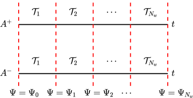
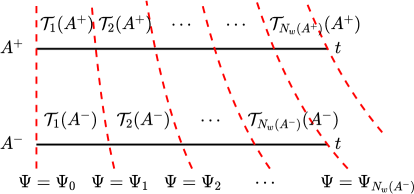
Figure 1 illustrates a possible scenario of the temporal domain partition for two generic testing parameters $A^{-},A^{+}\in\mathsf{D}$, where $A^{-}<A^{+}$, with two decomposition mechanisms which we are going to introduce in the rest of this section. It should be highlighted that the partition of the temporal domain is parameter-dependent if penetration distance is used as the indicator $\Psi$, while it is parameter-independent if physical time is used. This will be further explained in later subsections.

Fig. 1: Illustration of the parameter-dependence of temporal domain partition using physical time (left) and penetration distance (right) for manifold decomposition for two generic testing parameters $A^{-},A^{+}\in\mathsf{D}$, where $A^{-}<A^{+}$. Note that we have $N_{w}(A^{-})\leq N_{w}(A^{+})$.

4.2 Time-windowing: decomposition by physical time

A very natural choice of the indicator is the physical time, i.e. $\Psi(\boldsymbol{y},t,A)=t$. In that case, for any problem parameter $A\in\mathsf{D}$, we have $N_{w}(A)=N_{w}^{\text{off}}$ and $T_{j}(A)=\Psi_{j}$ for all $1\leq j\leq N_{w}^{\text{off}}$. In other words, the temporal partition is parameter-independent. As in the figure on the left in Figure 1, we can safely remove the parameter dependence and the superscript for distinguishing offline and online indices in the temporal domain partition. We remark that this choice reduces to the time-windowing (TW) reduced order model approach in Section 4 of [72].

One may decompose the temporal domain into windows using a prescribed partition, that is, the end points $\{\Psi_{j}\}_{j=1}^{N_{w}}$ are user-defined. Heuristically, the number of snapshots for a variable in a window is proportional to the window size if a uniform time step is used in the FOM simulation. In addition, if a uniform partition is used to decompose the domain into windows, then the basis sizes will be heuristically balanced among the windows. However, in the setting of adaptive time stepping, it becomes unclear how to prescribe window sizes to balance the ROM basis size among time windows. As an alternative, one can adaptively divide the temporal domain into windows using a prescribed number of snapshots per window, which can be heuristically related to the basis size. This adaptive decomposition approach is described in Algorithm 1 in the context of a general indicator $\Psi$ and is used in our numerical experiments in Section 5.

Algorithm 1 Adaptive partition of indicator range

1:Input:

• $\left\{(\boldsymbol{y}_{n}(A_{k}),t_{n}(A_{k}),A_{k}):0\leq n\leq N_{t}(A_{k})\text{ and }k\in{\rm Nature}{n_{A}}\right\}$, the collection of all snapshot triplets,

• $N_{\text{sample}}$, maximum number of intermediate samples in a subinterval for each offline parameter,

• $\Psi:\mathbb{R}^{N}\times\mathbb{R}^{+}\times\mathsf{D}\to\mathbb{R}$, the partition indicator,

• $[\Psi_{\text{min}},\Psi_{\text{max}})$, the range of the collection of all snapshot triplets under the indicator

2:Initilize $j=0$, $\Psi_{0}=\Psi_{\text{min}}$, $\mathcal{K}={\rm Nature}{n_{A}}$, and $n_{0}(A_{k})=0$ for all $k\in{\rm Nature}{n_{A}}$

3:repeat

4:     Increment $j\leftarrow j+1$

5:     for $k\in\mathcal{K}$ do

6:         Set $n_{j,{k}}^{\prime}=\min\{{n_{j-1}(A_{k})+N_{\text{sample}}+1},N_{t}(A_{k})\}$

7:         Set $\Psi_{j,k}=\Psi(\boldsymbol{y}_{n_{j,{k}}^{\prime}}(A_{k}),t_{n_{j,{k}}^{\prime}},A_{k})$

8:     end for

9:     Set the endpoint of the $j$-th subinterval as $\Psi_{j}=\min_{k\in\mathcal{K}}\Psi_{j,k}$

10:     Initialize the $j$-th snapshot index group by $\mathcal{G}_{j}=\emptyset$

11:     for $k\in\mathcal{K}$ do

12:         Set $n_{j}(A_{k})$ as the latest time index in the subinterval $\mathcal{T}_{j}$ for the offline parameter $A_{k}$ , i.e.

(4.11) $$\Psi(\boldsymbol{y}_{n_{j}(A_{k})}(A_{k}),t_{n_{j}(A_{k})},A_{k})\leq\Psi_{j}<\Psi(\boldsymbol{y}_{n_{j}(A_{k})+1}(A_{k}),t_{n_{j}(A_{k})+1},A_{k})$$

13:         Enrich the $j$-th snapshot index group by

(4.12) $$\mathcal{G}_{j}\leftarrow\mathcal{G}_{j}\cup\{(n,k)\in\mathbb{Z}\times{\rm Nature}{n_{A}}:n_{j-1}(A_{k})\leq n\leq n_{j}(A_{k})\}$$

14:         if $n_{j}(A_{k})=N_{t}(A_{k})$ then

15:              Remove $k$ from the index set of active training parameters by $\mathcal{K}\leftarrow\mathcal{K}\setminus\{k\}$

16:         end if

17:     end for

18:until $\mathcal{K}=\emptyset$

19:Set $N_{w}^{\text{off}}=j$ and verify $\Psi_{N_{w}^{\text{off}}}<\Psi_{\text{max}}$

20:Output:

• $N_{w}^{\text{off}}$, number of subintervals,

• $\{\Psi_{j}\}_{j=0}^{N_{w}^{\text{off}}}$, partition of indicator range, and

• $\{\mathcal{G}_{j}\}_{j=1}^{N_{w}^{\text{off}}}$, sequence of snapshot index groups

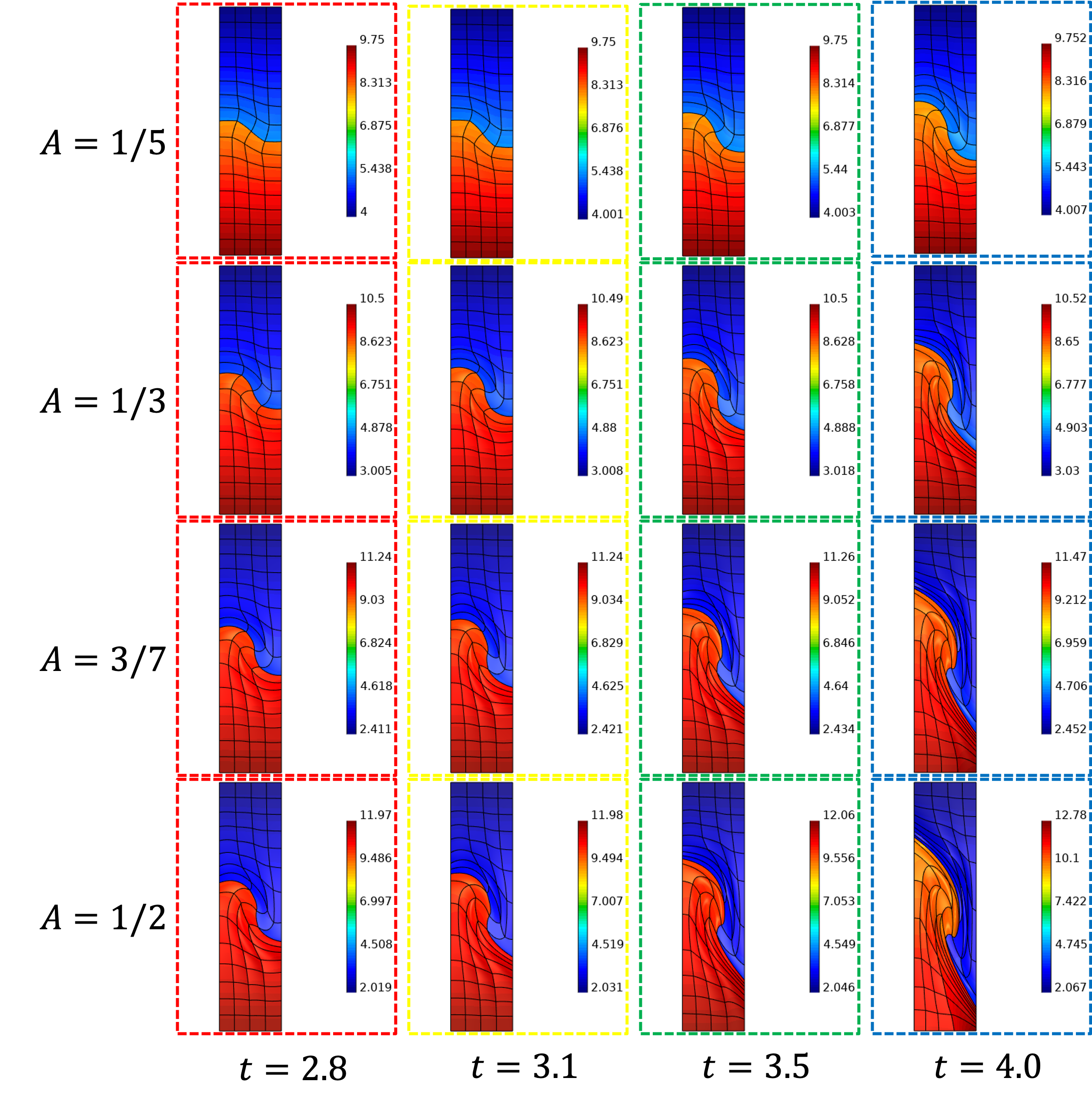
Figure 2 illustrates a possible scenario of the classification of snapshot samples with physical time being the indicator. The sixteen snapshot samples of the energy variable are collected from four different time instances and four different density ratio (and therefore problem parameter). With a sufficiently fine partition of the indicator range, i.e. the temporal domain, each one of the sixteen snapshot samples will belong to one of the four different groups, where the samples in each group are surrounded by a box with the same color, namely red, yellow, green, and blue. It can be seen that the fluid interface penetrates to different extents for the snapshot samples in the same group. This suggests that the linear dependence among the snapshots is weak, and it is difficult to achieve a linear subspace reduced basis with a small dimension, limiting speed-up.

Fig. 2: An illustrative example to explain the mechanism of decomposition of solution manifold using physical time as indicator. The samples collected at the same time instance belong to the same group. The samples in each group is surrounded by a box with the same color, namely red, yellow, green, and blue. Each group has weak linear dependence since the samples penetrate to different extents.

4.3 Distance windowing: decomposition by penetration distance

To reduce the size of the solution basis, we propose to use the downward penetration distance, which characterizes the Rayleigh-Taylor instability problem well. The penetration distance is defined as the largest downward displacement of the interface, i.e.,

(4.13) $$\Psi(\boldsymbol{y},t,A)=\max_{\widetilde{x}_{2}=0}x_{2}(\widetilde{x}),$$

where $x_{2}\in\mathbb{R}$ is the vertical component of the functional representation $x:\widetilde{\Omega}\rightarrow\mathbb{R}^{2}$ of the position vector $\boldsymbol{x}$ of a point on the interface, i.e., $\widetilde{x}_{2}=0$, where $\widetilde{x}$ is the Eulerian coordinates, or equivalently, the initial Lagrangian coordinates. We remark that, by taking the advantage of Lagrangian formulation of the Euler equations, the penetration distance is easily accessible. Since the penetration speed depends on the density ratio and hence the Atwood number, the temporal domain partition is parameter-dependent. The figure on the right in Figure 1 shows the temporal domain partition of two generic testing parameters $A^{-},A^{+}\in\mathsf{D}$, where $A^{-}<A^{+}$. With a higher Atwood number $A^{+}$, the fluid interface penetrates faster, and it takes shorter time for the penetration distance to reach the endpoints $\Psi_{j}$. This generates more but shorter subintervals in the temporal partition of $A^{+}$ than those of $A^{-}$, i.e. $N_{w}(A^{-})\leq N_{w}(A^{+})$. We name this approach distance-windowing (DW) reduced order model.

Again, one may decompose the indicator range of penetration distance into subintervals using a prescribed partition of the end points $\{T_{j}\}_{j=1}^{N_{w}}$. Besides the difficulties discussed in TW-ROM, the indicator range of penetration distance is not known prior to obtaining all the snapshots, and it is even more difficult to determine a good partition. Similar to the case of physical time, one can adaptively divide the indicator range of penetration distance into subintervals using a prescribed number of snapshots per window, which can be heuristically related to the basis size. Again, we refer the readers to Algorithm 1 for the details. The adaptive decomposition approach is used in our numerical experiments in Section 5.

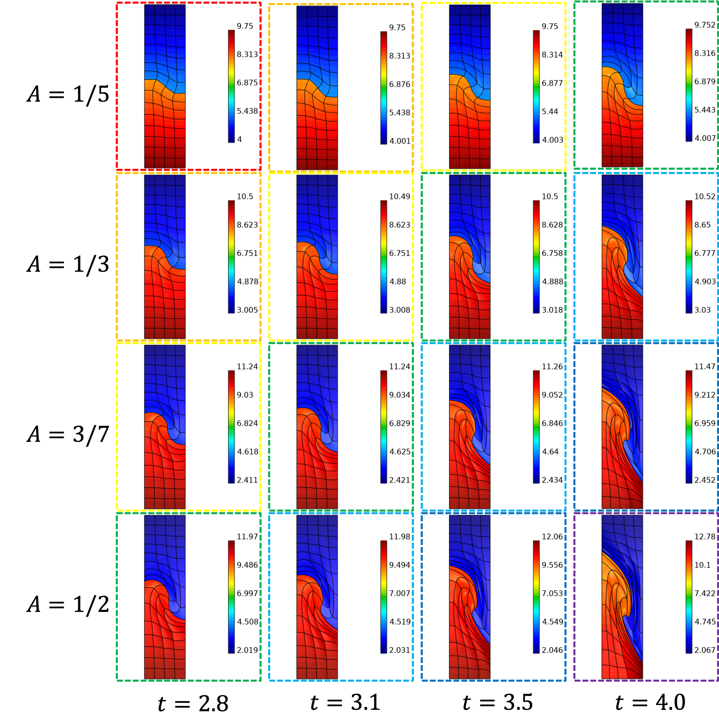
Figure 3 illustrates a possible scenario of the classification of snapshot samples with penetration distance being the indicator. Each one of the sixteen snapshot samples of the energy variable will belong to one of the seven different groups, where the samples in the same group are surrounded by a box with the same color, namely red, orange, yellow, green, cyan, blue, and purple. A sample collected at the earlier time instance with higher density ratio is associated with one collected at the later time instance with lower density ratio, since the penetration speed is slower with low density ratio. As we can observe, this choice of indicator provides much better linear dependence among the snapshots within the same group, as the fluid interface penetrates to a similar extent.

Fig. 3: An illustrative example to explain the mechanism of decomposition of solution manifold using penetration distance as indicator. The samples penetrating to similar extent belong to the same group. The samples in each group is surrounded by a box with the same color, namely red, orange, yellow, green, cyan, blue, and purple. Each group has strong linear dependence.

5 Numerical studies

In this section, we present numerical results to test the performance of our proposed method applied to Rayleigh–Taylor instability in Lagrangian hydrodynamics simulated with LaghosROM and libROM. LaghosROM is a C++ miniapp that accelerates time-dependent Euler equations of compressible gas dynamics in a moving Lagrangian frame using unstructured high-order finite element spatial discretization, explicit high-order time-stepping, and projection-based reduced order models. libROM is a C++ library for data-driven physical simulation methods [100]. All the simulations in this section use the machine Quartz in the Livermore Computing Center, on Intel Xeon CPUs with 128 GB memory, peak TFLOPS of 3251.4, and peak single CPU memory bandwidth of 77 GB/s.

We compare the ROM performance with different FOM discretization levels, ROM parameters, and decomposition mechanisms at different Atwood numbers. Algorithm 1 reports the adaptive decomposition mechanism in our implementation, where the indicator $\Psi$ is chosen as the physical time as in Section 4.2 or the penetration distance as in Section 4.3, with $N_{\text{sample}}$ being a user-defined constant to control the maximum number of intermediate samples to be added to a group for each training parameter. Moreover, the over-sampling factors $\{\lambda_{\breve{\mathsf{F}^{\mathfrak{1}}}},\lambda_{\breve{\mathsf{F}^{tv}}}\}$ are user-defined constants over all time windows, which control the number of sampling indices $n_{\breve{\mathsf{F}^{\mathfrak{1}}}}^{j}$ and $n_{\breve{\mathsf{F}^{tv}}}^{j}$ in the sampling matrices $\mathbf{Z}_{\mathsf{F}^{\mathfrak{1}}}^{j}$ and $\mathbf{Z}_{\mathsf{F}^{tv}}^{j}$ of the window $j$ by

(5.1) $$n_{\breve{\mathsf{F}^{\mathfrak{1}}}}^{j}=\min\left\{N_{\mathcal{V}},\,\lambda_{\breve{\mathsf{F}^{\mathfrak{1}}}}n_{\mathsf{F}^{\mathfrak{1}}}^{j}\right\},\quad n_{\breve{\mathsf{F}^{tv}}}^{j}=\min\left\{N_{\mathcal{E}},\,\lambda_{\breve{\mathsf{F}^{tv}}}n_{\mathsf{F}^{tv}}^{j}\right\},$$

where $n_{\mathsf{F}^{\mathfrak{1}}}^{j}$ and $n_{\mathsf{F}^{tv}}^{j}$ are the numbers of columns of the nonlinear term bases $\mathbf{\Phi}_{\mathsf{F}^{\mathfrak{1}}}^{j}$ and $\mathbf{\Phi}_{\mathsf{F}^{tv}}^{j}$, respectively. To evaluate the ROM performance, the relative error for each ROM field is measured against the corresponding FOM solution at the final time $t_{f}$, which is defined as:

(5.2) $$\mathcal{\epsilon}_{v,t_{f}} =\frac{\|\boldsymbol{v}_{N_{t}}-\tilde{\boldsymbol{v}}_{\widetilde{N}_{t}}\|_{2}}{\|\boldsymbol{v}_{N_{t}}\|_{2}}, \mathcal{\epsilon}_{e,t_{f}} =\frac{\|\boldsymbol{e}_{N_{t}}-\tilde{\boldsymbol{e}}_{\widetilde{N}_{t}}\|_{2}}{\|\boldsymbol{e}_{N_{t}}\|_{2}}, \mathcal{\epsilon}_{x,t_{f}} =\frac{\|\boldsymbol{x}_{N_{t}}-\tilde{\boldsymbol{x}}_{\widetilde{N}_{t}}\|_{2}}{\|\boldsymbol{x}_{N_{t}}\|_{2}}.$$

The speed-up of each ROM simulation is measured by dividing the wall-clock time for the FOM time loop by the wall-clock time for the corresponding ROM time loop.

5.1 Effects of FOM discretization

As a first experiment, we investigate the performance in terms of solution accuracy and speed-up of the ROM in the same problem set-up with different FOM discretization settings. The FOM discretization is set on different mesh refinement levels and the same finite element polynomial degree of 2 and 1 for the kinematic and thermodynamic space respectively, and hence the dimension of the finite element spaces asymptotically scales quadratically with the refinement level. The snapshots are taken at $n_{A}=1$ parameter, namely $A_{1}=1/3$, with the final time $t_{f}(A_{1})=1.5$. Table 1 summarizes the degress of freedom, number of time steps, and wall clock time in Rayleigh–Taylor instability problem with various mesh refinement level of FOM discretization.

Refinement level	2	3	4	5
$N_{\mathcal{V}}$	594	2210	8514	33410
$N_{\mathcal{E}}$	256	1024	4096	16384
$N_{t}$	435	926	1870	3780
FOM wall clock (seconds)	1.96	15.1	128	1010

Table 1: Degress of freedom, number of time steps, and wall clock time in Rayleigh–Taylor instability problem with varying FOM discretization.

In the offline phase, the fully discrete FOM scheme is first used to compute solution snapshots, which are classified into groups using the physical time as the indicator $\Psi$ (see Section 4.2). In practice, we start with $\Psi_{0}=0$, and sequentially determine the indicator range partition in the offline phase using Algorithm 1. We remark that, when $n_{A}=1$, according to (4.2), we have

(5.3) $$\mathcal{G}_{j}=\{(n,1)\in\mathbb{Z}\times\{1\}:n_{j-1}+1\leq n\leq\min\{n_{j-1}+N_{\text{sample}}+1,N_{t}\}\},$$

where we drop the notation of the dependence on $A_{1}$ for brevity. In this experiment, we take $N_{\text{sample}}=20$. Then for $1\leq j\leq N_{w}^{\text{off}}$, the reduced order model is constructed by performing POD on the subset of snapshots whose indices belong to the group $\mathcal{G}_{j}$. The oversampling ratio is taken as $\lambda_{\breve{\mathsf{F}^{\mathfrak{1}}}}=\lambda_{\breve{\mathsf{F}^{tv}}}=2$ in hyper-reduction. The offset vectors are taken as the initial state, i.e. $\boldsymbol{v}_{\text{os}}^{j}=\boldsymbol{v}(0)$, $\boldsymbol{e}_{\text{os}}^{j}=\boldsymbol{e}(0)$, and $\boldsymbol{x}_{\text{os}}^{j}=\boldsymbol{x}(0)$. The resultant reduced solution bases for velocity and energy are left-multiplied by the corresponding mass matrix to obtain the nonlinear term bases using SNS, which in turn determine the sampling indices by DEIM (see Section 3.3).

To avoid complicating the results, we fix all ROM parameters and consider only the reproductive case, i.e. the ROM simulation is performed at the same parameter $A=1/3$ and the final time $\widetilde{t}_{f}(A)=1.5$ in the online phase. To simplify the notation, we suppress the parameter dependence of all the notations in the remainder of this subsection, without introducing any ambiguity. In the online phase, the corresponding reduced order model is used, where the end-point $T_{j}(A)$ of the temporal subinterval $\mathcal{T}_{j}(A)$ is defined as the time instance $\widetilde{t}_{n}(A)$ when $\Psi(\tilde{\boldsymbol{y}}_{n}(A),\widetilde{t}_{n}(A),A)$ first exceeds $\Psi_{j}$, at which we increment to the next time subinterval $\mathcal{T}_{j+1}(A)$. The reduced basis and the sampling matrices are then used to formulate the hyper-reduced system (4.5) in each temporal subtinterval. The fully discrete hyper-reduced system follows from applying the RK2-average scheme.

Table 2 and Table 3 summarize the results in solution accuracy and speed-up of TW-ROM in Section 4.2 and DW-ROM in Section 4.3, respectively. In the short-time simulation, both TW-ROM and DW-ROM perform well, and they have similar level of solution accuaracy and speed-up. As the refinement level increases, the solution accuracy in all the variables remains outstanding. The relative error ranges from $O(10^{-7})$ to $O(10^{-3})$ and is not sensitive to the FOM discretization. Among the three solution components, the velocity has the largest relative error at the final time. In fact, the absolute error of the velocity and the specific internal energy has the same order of magnitude, but the order of the norm of the velocity is lower than that of the energy by 2. Meanwhile, the speed-up increases with the refinement level. While the FOM computational cost scales as a polynomial with the refinement level, the ROM computational expense mostly depends on the distribution of snapshot data and the ROM parameters, and is much less sensitive to the FOM discretization. The speed-up is very remarkable with higher refinement levels, for which the FOM simulations are more expensive. With the refinement level of 5, the speed-up is almost 50 times with both TW-ROM and DW-ROM.

Refinement level	2	3	4	5
$N_{w}$	44	93	187	379
$\widetilde{N}_{t}$	403	848	1841	3502
$\mathcal{\epsilon}_{v,t_{f}}$	4.2217e-03	4.5689e-03	4.1547e-02	2.8951e-03
$\mathcal{\epsilon}_{e,t_{f}}$	3.8508e-06	1.0837e-05	1.4926e-04	1.0660e-05
$\mathcal{\epsilon}_{x,t_{f}}$	9.4068e-06	9.1305e-07	2.7141e-04	2.7827e-05
speed-up	1.1058	3.4887	12.5000	48.6021

Table 2: TW-ROM performance comparison for short-time simulation in Rayleigh–Taylor instability problem with varying FOM discretization.

Refinement level	2	3	4	5
$N_{w}$	44	93	187	379
$\widetilde{N}_{t}$	403	848	1752	3584
$\mathcal{\epsilon}_{v,t_{f}}$	4.2217e-03	4.6212e-03	3.3420e-03	2.4819e-03
$\mathcal{\epsilon}_{e,t_{f}}$	3.8508e-06	1.0990e-05	8.6944e-06	5.7578e-06
$\mathcal{\epsilon}_{x,t_{f}}$	9.4068e-06	1.3922e-06	1.7685e-05	1.7119e-05
speed-up	1.0927	3.5467	12.0573	46.0935

Table 3: DW-ROM performance comparison for short-time simulation in Rayleigh–Taylor instability problem with varying FOM discretization.

5.2 Comparison of partition indicators for extrapolation

In this section, we investigate the performance in terms of solution accuracy and speed-up of the ROM with the different partition indicators at various Atwood numbers in the parametric problem setting. It should be emphasized that the parametric problem setting is challenging as the initial state depends on the density ratio $R$ and hence the Atwood number $A$, and has a significant influence on the highly nonlinear dynamics. The FOM discretization is set on the same mesh refinement level of 4 and the same finite element polynomial degree of 2 and 1 for the kinematic and thermodynamic space respectively. We follow the same procedure as in Section 5.1 for sampling snapshots, decomposing the indicator range, constructing bases in the offline phase, and ROM simulation in the online phase.

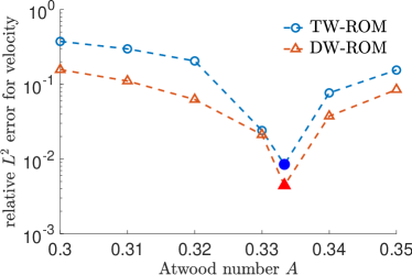
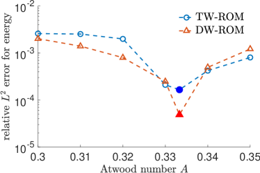
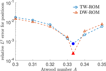
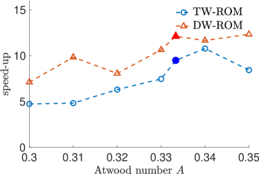
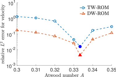
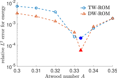
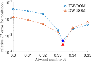
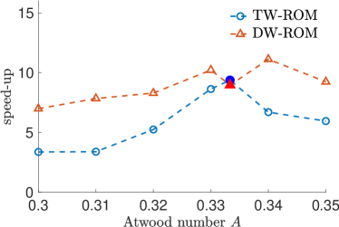
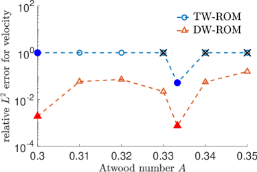
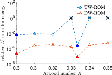
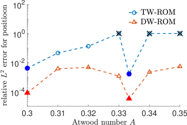
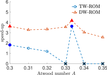
In the first experiment, we use $n_{A}=1$ training parameter, namely $A_{1}=1/3$, with the final time $t_{f}(A_{1})=3.2$ for snapshot sampling. We take $N_{\text{sample}}=20$ for decomposing the indicator range by Algorithm 1, and $\delta_{\sigma}\in\{10^{-4},10^{-10}\}$ for performing proper orthogonal decomposition. The ROM simulation is performed at the various parameters $A\in\mathsf{D}=[0.3,0.35]$ with final time $\widetilde{t}_{f}(A)\equiv 3$ and the oversampling ratio $\lambda_{\breve{\mathsf{F}^{\mathfrak{1}}}}=\lambda_{\breve{\mathsf{F}^{tv}}}=5$ for hyper-reduction in the online phase. Figure 4 and Figure 5 show the results in solution accuracy and speed-up with $\delta_{\sigma}=10^{-4}$ and $\delta_{\sigma}=10^{-10}$ respectively. The filled markers correspond to the reproductive case, i.e. $A=A_{1}=1/3$, while the other markers correspond to extrapolatory cases at selected testing points $A\in\mathsf{D}\setminus\{A_{1}\}$. The results of TW-ROM, i.e. using physical time as the indicator in Section 4.2, and DW-ROM, i.e. using penetration distance as the indicator in Section 4.3, are depicted in blue and red, respectively. From the error plots for all the solution fields, it can be observed that the solution accuracy degenerates when the testing points are farther away from the training point $A_{1}=1/3$, in both cases of using the physical time or penetration distance as the indicator $\Psi$. Both approaches provide an acceptable solution accuracy at the reproductive case $A=1/3$, and using the penetration distance gives better results, where the error in velocity is less than 1%. However, the approaches have significantly different performance at the extrapolatory cases which are of greater interest in the practical use of reduced order models. The numerical results show that the physical time indicator generally has worse accuracy, especially for the velocity field at the extrapolatory cases, where the error at $A\in[0.3,0.32]$ are higher than 40% with $\delta_{\sigma}=10^{-4}$ as shown in Figure 4, and almost 100% with $\delta_{\sigma}=10^{-10}$ as shown in Figure 5. On the other hand, the penetration distance is a more reliable indicator to assign the reduced order model in the online phase for extrapolatory parameters in general, especially for lower Atwood numbers $A\in[0.3,0.32]$. Moreover, the penetration distance indicator is superior to the physical time indicator in terms of speed-up.

Fig. 4: Extrapolation test: ROM performance comparison for long-time simulation in Rayleigh–Taylor instability problem at varying Atwood number with $n_{A}=1$ and $\delta_{\sigma}=10^{-4}$: relative $L^{2}$ error for velocity (top-left), relative $L^{2}$ error for energy (top-right), relative $L^{2}$ error for position (bottom-left), and speed-up (bottom-right). Using the penetration distance improves the solution accuracy at the extrapolatory cases.

Fig. 5: Extrapolation test: ROM performance comparison for long-time simulation in Rayleigh–Taylor instability problem at varying Atwood number with $n_{A}=1$ and $\delta_{\sigma}=10^{-10}$: relative $L^{2}$ error for velocity (top-left), relative $L^{2}$ error for energy (top-right), relative $L^{2}$ error for position (bottom-left), and speed-up (bottom-right). Using the penetration distance improves the solution accuracy at the extrapolatory cases.

In the second experiment, we use $n_{A}=2$ training parameters, namely $A_{1}=1/3$ and $A_{2}=0.3$, with the final time $t_{f}(A_{1})=t_{f}(A_{2})=3.2$ for snapshot sampling. We take $N_{\text{sample}}=20$ for decomposing the indicator range by Algorithm 1, and $\delta_{\sigma}=10^{-10}$ for performing proper orthogonal decomposition. The ROM simulation is performed at the various parameters $A\in\mathsf{D}=[0.3,0.35]$ with final time $\widetilde{t}_{f}(A)\equiv 3$ and the oversampling ratio $\lambda_{\breve{\mathsf{F}^{\mathfrak{1}}}}=\lambda_{\breve{\mathsf{F}^{tv}}}=10$ for hyper-reduction in the online phase. Figure 6 shows the solution accuracy and speed-up. The filled markers correspond to the reproductive case, i.e. $A\in\{A_{1},A_{2}\}$, while the other markers correspond to extrapolatory cases at selected testing points $A\in\mathsf{D}\setminus\{A_{1},A_{2}\}$ that do not contribute snapshot samples to the basis construction in the offline phase. The results of TW-ROM, i.e. using physical time as the indicator in Section 4.2, and DW-ROM, i.e. using penetration distance as the indicator in Section 4.3, are depicted in blue and red, respectively. In this experiment, using the physical time as the indicator yields numerical instability, which is due to poor approximation properties of the reduced subspaces. It is therefore evidential that the decomposition of the solution manifold by the physical time does not produce submanifolds with small Kolmogorov $n$-width. The unstable cases at $A\in\{0.33,0.34,0.35\}$ are indicated by the crossed markers with a 100% error and zero speed-up in the blue line plot corresponding to TW-ROM. Even at the stable cases, the error in velocity is almost 100%, which again suggests that using the physical time does not provide good approximation for the velocity. Meanwhile, using the penetration distance as the indicator produces reasonable results. The error in the solution attains local minima at the training parameters $\{A_{1},A_{2}\}$, and grows as the testing parameter $A$ gets farther away from the training parameters.

Fig. 6: ROM performance comparison for long-time simulation in Rayleigh–Taylor instability problem at varying Atwood number with $n_{A}=2$ and $\delta_{\sigma}=10^{-10}$: relative $L^{2}$ error for velocity (top-left), relative $L^{2}$ error for energy (top-right), relative $L^{2}$ error for position (bottom-left), and speed-up (bottom-right). Using the penetration distance improves the solution accuracy and stability at the extrapolatory cases.

5.3 Comparison of partition indicators on final time

In this experiment, we investigate the performance of the ROM with the different partition indicators at different time instances in an extrapolatory problem setting. The final time is chosen to be sufficiently long for the instability to develop into a highly nonlinear regime with the formation of a vortex at the fluid interface. The FOM discretization is set on the same mesh refinement level of 4 and the same finite element polynomial degree of 2 and 1 for the kinematic and thermodynamic spaces, respectively. The procedure of building and applying the reduced order model follows exactly as in Section 5.1. We use $n_{A}=1$ training parameter, namely $A_{1}=1/3$, with the final time $t_{f}(A_{1})=3.6$ for snapshot sampling. We take $N_{\text{sample}}=20$ for decomposing the indicator range by Algorithm 1. The ROM simulation is performed at the unseen parameter $A=0.33$ with various final time $\widetilde{t}_{f}(A)\in[3.0,3.6]$ and the oversampling ratio $\lambda_{\breve{\mathsf{F}^{\mathfrak{1}}}}=\lambda_{\breve{\mathsf{F}^{tv}}}=2$ for hyper-reduction in the online phase. To avoid complicating the results, we fix all ROM parameters.

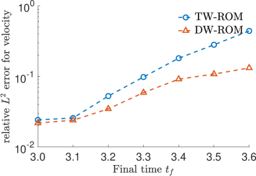
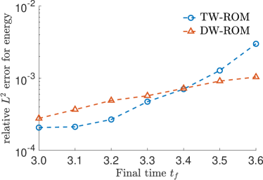
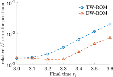
Figure 7 shows the results in terms of solution accuracy and speed-up. The results of TW-ROM, i.e. using physical time as the indicator in Section 4.2, and DW-ROM, i.e. using penetration distance as the indicator in Section 4.3, are depicted in blue and red, respectively. It can be seen that the solution error accumulates with time in both decomposition mechanisms. At the final time $t_{f}=3.6$, the error in velocity is around 44% when the physical time is used as the indicator, while it is around 13% when the penetration distance is used. These results highlight the importance of an appropriate indicator for accurate local ROM approximation, especially in highly complex nonlinear dynamics, such as the long-time simulation of Rayleigh–Taylor instability with the formation of vortices. As we will see in Section 5.4, the solution accuracy can be further improved by adding more samples in hyper-reduction when the penetration distance is used as the indicator. It is also important to point out that when the penetration distance is used as the indicator, a speed-up of 12-15 times is achieved at varying time instances, which are higher than 8-12 times when the physical time is used.

Fig. 7: ROM performance comparison for long-time simulation in Rayleigh–Taylor instability problem with varying final time: relative $L^{2}$ error for velocity (top-left), relative $L^{2}$ error for energy (top-right), relative $L^{2}$ error for position (bottom-left), and speed-up (bottom-right). Using the penetration distance improves the solution accuracy and speed-up at all tested oversampling ratio.

5.4 Comparison of partition indicators on oversampling ratio

In this experiment, we further investigate the performance of the ROM with the different partition indicators and various oversampling ratios of hyper-reduction in an extrapolatory problem setting. The final time is set to be sufficiently long to allow the formation of a vortex at the fluid interface in the highly nonlinear dynamics. The FOM discretization is set on the same mesh refinement level of 4 and the same finite element polynomial degree of 2 and 1 for the kinematic and thermodynamic spaces, respectively. The procedure of building and applying the reduced order model follows exactly as in Section 5.1. We use $n_{A}=1$ training parameter, namely $A_{1}=1/3$, with the final time $t_{f}(A_{1})=3.6$ for snapshot sampling.

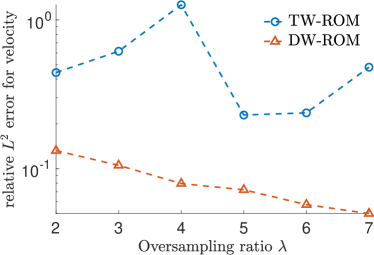
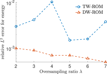
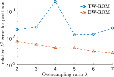
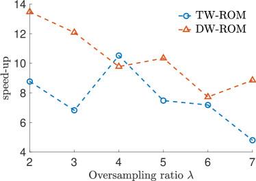
First, we take $N_{\text{sample}}=20$ for decomposing the indicator range by Algorithm 1. The ROM simulation is performed at the unseen parameter $A=0.33$ with final time $\widetilde{t}_{f}(A)=3.6$ and varying oversampling ratio $\lambda_{\breve{\mathsf{F}^{\mathfrak{1}}}}=\lambda_{\breve{\mathsf{F}^{tv}}}=\lambda\in[2,7]$ for hyper-reduction in the online phase. To avoid complicating the results, we fix all ROM parameters except the oversampling ratio. Figure 8 shows the results in terms of solution accuracy and speed-up with $N_{\text{sample}}=20$ and various oversampling ratio $\lambda$. The results of TW-ROM, i.e. using physical time as the indicator in Section 4.2, and DW-ROM, i.e. using penetration distance as the indicator in Section 4.3, are depicted in blue and red, respectively. It can be seen that using the penetration distance as the indicator does not only provide more accurate approximation in all the solution variables but also better speed-up in the ROM simulation compared to using the physical time. Moreover, when the penetration distance is used, we can observe a decaying trend in the solution error and speed-up with increasing oversampling ratio $\lambda$, which provides a tuneable solution accuracy against the computational expense. On the other hand, the solution accuracy does not necessarily improve with increasing oversampling ratio $\lambda$ when the physical time is used. At the oversampling ratio $\lambda=7$, the error in velocity is around 48% when the physical time is used as the indicator, while it is around 5% when the penetration distance is used.

Fig. 8: ROM performance comparison for long-time simulation in Rayleigh–Taylor instability problem with varying oversampling ratio: relative $L^{2}$ error for velocity (top-left), relative $L^{2}$ error for energy (top-right), relative $L^{2}$ error for position (bottom-left), and speed-up (bottom-right). Using the penetration distance improves the solution accuracy and speed-up at all tested oversampling ratio.

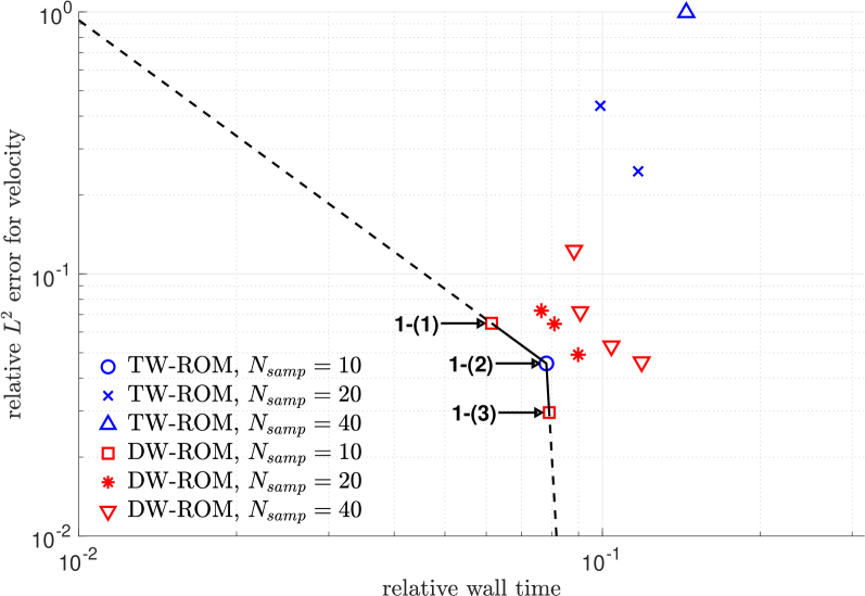
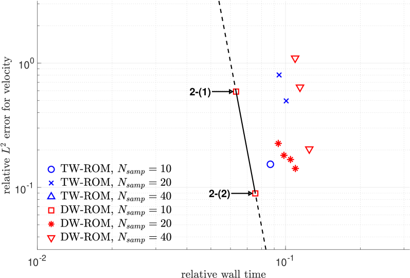
Finally, we provide a thorough comparison of different choices in ROM simulation. We use different combinations of indicator and $N_{\text{sample}}\in\{10,20,40\}$ in Algorithm 1. Again, the ROM simulation is performed at the unseen parameter $A=\{0.32,0.33\}$ with final time $\widetilde{t}_{f}(A)=3.6$ and varying oversampling ratio $\lambda_{\breve{\mathsf{F}^{\mathfrak{1}}}}=\lambda_{\breve{\mathsf{F}^{tv}}}=\lambda\in[2,7]$ for hyper-reduction in the online phase. In Figure 9 and Figure 10, we construct a Pareto front, which is characterized by the ROM user-defined input values that minimize the competing objectives of relative $L^{2}$ error for velocity and relative wall time, with all the combinations of ROM parameters at $A=0.33$ and $A=0.32$, respectively. It can be observed that using the penetration distance as the indicator performs better in general, and the error is less sensitive to the number of intermediate samples in a subinterval $N_{\text{sample}}$. Meanwhile, the error increases dramatically with $N_{\text{sample}}$ when the physical time is used as the indicator. Moreover, with $A=0.32$ and $N_{\text{sample}}=40$, TW-ROM is numerically unstable with any choice of oversampling ratio $\lambda$. An overall Pareto front that selects the ROM parameters that are Pareto-optimal across all groups is also illustrated. Table 4 reports the ROM user-defined input values that yielded the results on the overall Pareto fronts. The results of this experiment also suggest that the penetration distance is a more reliable indicator than the physical time to produce a remarkable speed-up as well as accurate approximations with the appropriate use of hyper-reduction.

Fig. 9: ROM performance comparison for long-time simulation in Rayleigh–Taylor instability problem at $A=0.33$ with varying oversampling ratio. Relative $L^{2}$ error for velocity versus relative wall time for varying ROM parameters.

Fig. 10: ROM performance comparison for long-time simulation in Rayleigh–Taylor instability problem at $A=0.32$ with varying oversampling ratio. Relative $L^{2}$ error for velocity versus relative wall time for varying ROM parameters.

Label	1-(1)	1-(2)	1-(3)	2-(1)	2-(2)
Decomposition	DW	TW	DW	DW	DW
$N_{\text{sample}}$	10	10	10	10	10
$\lambda$	2	2	4	2	4

Table 4: ROM user-defined input values yielding Pareto-optimal performance for long-time simulation in the Rayleigh–Taylor instability problem with varying oversampling ratio. Figure 9–10 provide labels.

6 Conclusion

In this paper, we have developed reduced order model techniques to accelerate the simulation of Rayleigh–Taylor instability in compressible gas dynamics. The Euler equation is used to model the compressible gas dynamics in a complex multimaterial setting. Moreover, we study the effects of Atwood number as a problem parameter on the physical quantities. Using the curvilinear finite element method for solving the governing equations in a moving Lagrangian frame, the numerical solutions of Rayleigh–Taylor instability are accurate but computationally expensive. We use POD for solution basis construction and SNS and DEIM for hyper-reduction. Furthermore, we introduce a general framework for the temporal domain partition and temporally-local reduced order model construction with varying Atwood number. We compare two approaches in this framework, namely decomposing the solution manifold by physical time and penetration distance respectively. Numerical results show that the penetration distance indicator provides better results than the physical time indicator, in terms of both speed-up and solution accuracy. In the future, we will carry out further investigation on reliable indicators for parameter-dependent temporal domain partition which lead to efficient reduced order models for advection-dominated problems. Although this work focused on a single parameter specific to the application, the general methodology can in principle be extended to other parameters for other problems.

Disclaimer

This document was prepared as an account of work sponsored by an agency of the United States government. Neither the United States government nor Lawrence Livermore National Security, LLC, nor any of their employees makes any warranty, expressed or implied, or assumes any legal liability or responsibility for the accuracy, completeness, or usefulness of any information, apparatus, product, or process disclosed, or represents that its use would not infringe privately owned rights. Reference herein to any specific commercial product, process, or service by trade name, trademark, manufacturer, or otherwise does not necessarily constitute or imply its endorsement, recommendation, or favoring by the United States government or Lawrence Livermore National Security, LLC. The views and opinions of authors expressed herein do not necessarily state or reflect those of the United States government or Lawrence Livermore National Security, LLC, and shall not be used for advertising or product endorsement purposes.

Appendix A Command line options of LaghosROM

For the purpose of reproducible research, we present some examples of the command line options for simulating the Rayleigh–Taylor instability problem using LaghosROM. Due to rapid software development in the repository, the commands lines are subject to change. However, we try our best to present the command lines compatible with recent versions of different dependent softwares and maintain a simple usage of the program. The following command lines are compatible with the recent commits of the master branch of MFEM , the master branch of libROM , and the rom branch of Laghos . In order to use the ROM capability of Laghos, a user has to navigate to the rom subdirectory.

A.1 Problem specification

First, we present the commands lines for the FOM user-defined input values reported in Section 5 using the executable laghos. These command lines can also be used along with command line options for ROM user-defined input values. We use the long-time simulation for illustration. The following command line is used to specify the full-order Rayleigh-Taylor instability problem with the final time $t_{f}=3.6$, refinement level of 4, and the same finite element polynomial degree of 2 and 1 for the kinematic and thermodynamic space respectively.

./laghos -p 7 -m data/rt2D.mesh -s 7 -tf 3.6 -rs 4 -ok 2 -ot 1

This basic command line is appended by different options in different stages, namely computing FOM reference solution, sampling snapshots, constructing reduced basis and operators, computing ROM solution, and evaluating error. For computing FOM reference solution at the testing Atwood number $A=0.33$ to evaluate the error of the ROM solution obtained in Section A.3, one appends

-writesol -af 0.33

A.2 Offline computations

Next, we present the command line options for the offline ROM construction in Rayleigh-Taylor instability problem, which involves sampling snapshots and constructing reduced basis. The options are appended to the command lines for specifying the full-order problem in Section A.1. To build the ROM with one training Atwood number $A_{1}=1/3$, and using penetration distance as the indicator and $N_{\text{sample}}=20$ in Algorithm 1, one appends

-offline -romsns -ef 0.9999 -sample-stages -nwinsamp 21 -loctype distance

Here and thereafter, one drops -loctype distance in all the command lines for using physical time as the indicator instead.

On the other hand, to build the ROM with two training Atwood number $A_{1}=1/3$ and $A_{2}=0.3$, one appends

-offline -romsns -sample-stages -rpar 0 -sdim 200000 -loctype distance
-offline -romsns -sample-stages -rpar 1 -af 0.3 -sdim 200000 -loctype distance

and then uses a separate executable merge

./merge -nset 2 -romsns -ef 0.9999 -nwinsamp 21 -loctype distance

A.3 Online computations

Finally, we present the command line options for the online ROM simulation in Rayleigh-Taylor instability problem, which involves constructing reduced operators, computing ROM solution and evaluating error. The options are appended to the command lines for specifying the full-order problem in Section A.1. Below we present the ROM commands for using SNS hyper-reduction with over-sampling ratio $\lambda_{\breve{\mathsf{F}^{\mathfrak{1}}}}=\lambda_{\breve{\mathsf{F}^{tv}}}=2$ on $N_{w}^{\text{off}}=3863$ subintervals in the indicator range (from Algorithm 1) at the testing Atwood number $A=0.33$. For hyper-reduction preprocessing in the online phase, one appends

-online -romhrprep -romsns -sfacv 2 -sface 2 -nwin 3863 -af 0.33 -loctype distance

For ROM simulation in the online phase, one appends

-online -romhr -romsns -sfacv 2 -sface 2 -nwin 3863 -af 0.33 -loctype distance

Finally, for solution postprocessing and calculating the relative error between the FOM solution and the ROM solution, one appends

-restore -soldiff -romsns -nwin 3863 -af 0.33 -loctype distance

References

- [1] Lord Rayleigh. Investigation of the character of the equilibrium of an incompressible heavy fluid of variable density. Proceedings of the London Mathematical Society, s1–14:170–177, 1882.
- [2] Geoffrey Ingram Taylor. The instability of liquid surfaces when accelerated in a direction perpendicular to their planes. i. Proceedings of the Royal Society A, 201:192–196, 1950.
- [3] M. Livio, J.R. Buchler, and S.A. Colgate. Rayleigh–Taylor driven supernova explosions: A two-dimensional numerical study. The Astrophysical Journal, 238:L139–L143, 1980.
- [4] S. Yamada and K. Sato. Rayleigh–Taylor instability in the asymmetric supernova explosion. The Astrophysical Journal, 382:592–602, 1991.
- [5] John M. Blondin and Donald C. Ellison. Rayleigh–Taylor instabilities in young supernova remnants undergoing efficient particle acceleration. The Astrophysical Journal, 560:244–253, 2001.
- [6] X. Ribeyre and V.T. Tikhonchuk. Compressible Rayleigh–Taylor instabilities in supernova remnants. Physics of Fluids, 16:4661–4670, 2004.
- [7] M.J. Keskinen, E.P. Szuszczewicz, S.L. S. L. Ossakow, and J.C. Holmes. Nonlinear theory and experimental observations of the local collisional Rayleigh–Taylor instability in a descending equatorial spread ionosphere. Journal of Geophysical Research, 86:5785–5792, 1981.
- [8] C.-S. Huang, M.C. Kelley, and D.L. Hysell. Nonlinear Rayleigh–Taylor instabilities, atmospheric gravity waves and equatorial spread . Journal of Geophysical Research, 98:15631–15642, 1993.
- [9] W.S.D. Wilcock and J.A. Whitehead. Nonlinear Rayleigh–Taylor instabilities, atmospheric gravity waves and equatorial spread . Journal of Geophysical Research, 96:12193–12200, 1991.
- [10] H.-P. Plag and H.-U. Jüttner. Rayleigh–Taylor instabilities of a self-gravitating earth. Journal of Geodynamics, 20:267–288, 1995.
- [11] C.P. Conrad and P. Molnar. The growth of Rayleigh–Taylor-type instabilities in the lithosphere for various rheological and density structures. Geophysical Journal International, 129:95–112, 1997.
- [12] R. Betti, V.N. V. N. Goncharov, R.L. McCrory, and C.P. Verdon. Growth rates of the ablative Rayleigh–Taylor instability in inertial confinement fusion. Physics of Plasmas, 5:1446–1454, 1998.
- [13] Bruce A. Remington, Hye-Sook Park, Daniel T. Casey, Robert M. Cavallo, Daniel S. Clark, Channing M. Huntington, Carolyn C. Kuranz, Aaron R. Miles, Sabrina R. Nagel, Kumar S. Raman, and Vladimir A. Smalyuk. Rayleigh–Taylor instabilities in high-energy density settings on the national ignition facility. Proceedings of the National Academy of Sciences of the United States of America, 116(37):18233–18238, 2019.
- [14] S. Chandrasekhar. Hydrodynamic and Hydromagnetic Stability. Oxford University Press, Oxford, 1961.
- [15] D.H. Sharp. An overview of Rayleigh–Taylor instability. Physica D: Nonlinear Phenomena, 12:3–18, 1984.
- [16] A. Casner, C. Mailliet, G. Rigon, S.F. Khan, D. Martinez, B. Albertazzi, T. Michel, T. Sano, Y. Sakawa, P. Tzeferacos, D. Lamb, S. Liberatore, N. Izumi, D. Kalantar, P. Di Nicola, J.M. Di Nicola, E. Le Bel, I. Igumenshchev, V. Tikhonchuk, B.A. Remington, J. Ballet, E. Falize, L. Masse, V.A. Smalyuk, and M. Koenig. From icf to laboratory astrophysics: ablative and classical Rayleigh–Taylor instability experiments in turbulent-like regimes. Nuclear Fusion, 59:032002, 2018.
- [17] G. Tryggvason and S.O. Unverdi. Computations of three-dimensional Rayleigh–Taylor instability. Physics of Fluids A: Fluid Dynamics, 2:656–659, 1990.
- [18] David L. Youngs. Three‐dimensional numerical simulation of turbulent mixing by Rayleigh–Taylor instability. Physics of Fluids A: Fluid Dynamics, 3:1312–1320, 1991.
- [19] David L. Youngs. A comparative study of the turbulent Rayleigh–Taylor instability using high-resolution three-dimensional numerical simulations: The alpha-group collaboration. Journal of Physics, 16:1668–1693, 2004.
- [20] Hyun Geun Lee and Junseok Kim. Numerical simulation of the three-dimensional Rayleigh–Taylor instability. Computers & Mathematics with Applications, 66:1466–1474, 2013.
- [21] R. Zanella, G. Tegze, R. Le Tellier, and H. Henry. Two- and three-dimensional simulations of Rayleigh–Taylor instabilities using a coupled cahn–hilliard/navier–stokes model. Physics of Fluids, 32:124115, 2020.
- [22] Veselin A Dobrev, Tzanio V Kolev, and Robert N Rieben. High-order curvilinear finite element methods for Lagrangian hydrodynamics. SIAM Journal on Scientific Computing, 34(5):B606–B641, 2012.
- [23] Shun Wang, Eric de Sturler, and Glaucio H Paulino. Large-scale topology optimization using preconditioned Krylov subspace methods with recycling. International journal for numerical methods in engineering, 69(12):2441–2468, 2007.
- [24] Miguel A Salazar de Troya and Daniel A Tortorelli. Three-dimensional adaptive mesh refinement in stress-constrained topology optimization. Structural and Multidisciplinary Optimization, 62(5):2467–2479, 2020.
- [25] Miguel A Salazar De Troya and Daniel A Tortorelli. Adaptive mesh refinement in stress-constrained topology optimization. Structural and Multidisciplinary Optimization, 58(6):2369–2386, 2018.
- [26] Daniel A White, Youngsoo Choi, and Jun Kudo. A dual mesh method with adaptivity for stress-constrained topology optimization. Structural and Multidisciplinary Optimization, 61(2):749–762, 2020.
- [27] Youngsoo Choi, Charbel Farhat, Walter Murray, and Michael Saunders. A practical factorization of a Schur complement for PDE-constrained distributed optimal control. Journal of Scientific Computing, 65(2):576–597, 2015.
- [28] Young Soo Choi. Simultaneous analysis and design in PDE-constrained optimization. PhD thesis, Stanford University, 2012.
- [29] Ralph C Smith. Uncertainty quantification: theory, implementation, and applications, volume 12. Siam, 2013.
- [30] Lorenz Biegler, George Biros, Omar Ghattas, Matthias Heinkenschloss, David Keyes, Bani Mallick, Luis Tenorio, Bart van Bloemen Waanders, Karen Willcox, and Youssef Marzouk. Large-scale inverse problems and quantification of uncertainty, volume 712. John Wiley & Sons, 2011.
- [31] David Galbally, Krzysztof Fidkowski, Karen Willcox, and Omar Ghattas. Non-linear model reduction for uncertainty quantification in large-scale inverse problems. International journal for numerical methods in engineering, 81(12):1581–1608, 2010.
- [32] Chi Hoang, Youngsoo Choi, and Kevin Carlberg. Domain-decomposition least-squares Petrov-Galerkin (DD-LSPG) nonlinear model reduction. Computer methods in applied mechanics and engineering, 384:113997, 2021.
- [33] Felix Fritzen, Bernard Haasdonk, David Ryckelynck, and Sebastian Schöps. An algorithmic comparison of the hyper-reduction and the discrete empirical interpolation method for a nonlinear thermal problem. Mathematical and computational applications, 23(1):8, 2018.
- [34] Youngsoo Choi and Kevin Carlberg. Space–time least-squares Petrov–Galerkin projection for nonlinear model reduction. SIAM Journal on Scientific Computing, 41(1):A26–A58, 2019.
- [35] Youngsoo Choi, Deshawn Coombs, and Robert Anderson. SNS: a solution-based nonlinear subspace method for time-dependent model order reduction. SIAM Journal on Scientific Computing, 42(2):A1116–A1146, 2020.
- [36] Kevin Carlberg, Youngsoo Choi, and Syuzanna Sargsyan. Conservative model reduction for finite-volume models. Journal of Computational Physics, 371:280–314, 2018.
- [37] Rambod Mojgani and Maciej Balajewicz. Lagrangian basis method for dimensionality reduction of convection dominated nonlinear flows. arXiv preprint arXiv:1701.04343, 2017.
- [38] Youngkyu Kim, Karen May Wang, and Youngsoo Choi. Efficient space-time reduced order model for linear dynamical systems in Python using less than 120 lines of code. Mathematics, 9(14):1690, 2021.
- [39] Dunhui Xiao, Fangxin Fang, Andrew G Buchan, Christopher C Pain, Ionel Michael Navon, Juan Du, and G Hu. Non-linear model reduction for the navier–Stokes equations using residual deim method. Journal of Computational Physics, 263:1–18, 2014.
- [40] John Burkardt, Max Gunzburger, and Hyung-Chun Lee. POD and CVT-based reduced-order modeling of Navier–Stokes flows. Computer methods in applied mechanics and engineering, 196(1-3):337–355, 2006.
- [41] David Amsallem, Matthew Zahr, Youngsoo Choi, and Charbel Farhat. Design optimization using hyper-reduced-order models. Structural and Multidisciplinary Optimization, 51(4):919–940, 2015.
- [42] Youngsoo Choi, Gabriele Boncoraglio, Spenser Anderson, David Amsallem, and Charbel Farhat. Gradient-based constrained optimization using a database of linear reduced-order models. Journal of Computational Physics, 423:109787, 2020.
- [43] Youngsoo Choi, Geoffrey Oxberry, Daniel White, and Trenton Kirchdoerfer. Accelerating design optimization using reduced order models. arXiv preprint arXiv:1909.11320, 2019.
- [44] Sean McBane and Youngsoo Choi. Component-wise reduced order model lattice-type structure design. Computer methods in applied mechanics and engineering, 381:113813, 2021.
- [45] Mohamadreza Ghasemi and Eduardo Gildin. Localized model reduction in porous media flow. IFAC-PapersOnLine, 48(6):242–247, 2015.
- [46] Rui Jiang and Louis J Durlofsky. Implementation and detailed assessment of a GNAT reduced-order model for subsurface flow simulation. Journal of Computational Physics, 379:192–213, 2019.
- [47] Yanfang Yang, Mohammadreza Ghasemi, Eduardo Gildin, Yalchin Efendiev, Victor Calo, et al. Fast multiscale reservoir simulations with pod-deim model reduction. SPE Journal, 21(06):2–141, 2016.
- [48] Min Wang, Siu Wun Cheung, Eric T. Chung, Maria Vasilyeva, and Yuhe Wang. Generalized multiscale multicontinuum model for fractured vuggy carbonate reservoirs. Journal of Computational and Applied Mathematics, 366:112370, 2020.
- [49] Huanhuan Yang and Alessandro Veneziani. Efficient estimation of cardiac conductivities via POD-DEIM model order reduction. Applied Numerical Mathematics, 115:180–199, 2017.
- [50] Hongfei Fu, Hong Wang, and Zhu Wang. POD/DEIM reduced-order modeling of time-fractional partial differential equations with applications in parameter identification. Journal of Scientific Computing, 74(1):220–243, 2018.
- [51] Pengfei Zhao, Cai Liu, and Xuan Feng. POD-DEIM based model order reduction for the spherical shallow water equations with Turkel-Zwas finite difference discretization. Journal of Applied Mathematics, 2014, 2014.
- [52] R Ştefănescu and Ionel Michael Navon. POD/DEIM nonlinear model order reduction of an ADI implicit shallow water equations model. Journal of Computational Physics, 237:95–114, 2013.
- [53] Youngsoo Choi, Peter Brown, Bill Arrighi, Roberti Anderson, and Kevin Huynh. Space-time reduced order model for large-scale linear dynamical systems with application to Boltzmann transport problems. Journal of Computational Physics, 424:109845, 2021.
- [54] M Mordhorst, Timm Strecker, D Wirtz, Thomas Heidlauf, and Oliver Röhrle. POD-DEIM reduction of computational EMG models. Journal of Computational Science, 19:86–96, 2017.
- [55] Gabriel Dimitriu, Ionel M Navon, and Răzvan Ştefănescu. Application of POD-DEIM approach for dimension reduction of a diffusive predator-prey system with allee effect. In International conference on large-scale scientific computing, pages 373–381. Springer, 2013.
- [56] Harbir Antil, Matthias Heinkenschloss, Ronald HW Hoppe, Christopher Linsenmann, and Achim Wixforth. Reduced order modeling based shape optimization of surface acoustic wave driven microfluidic biochips. Mathematics and Computers in Simulation, 82(10):1986–2003, 2012.
- [57] Ming-C Cheng. A reduced-order representation of the Schrödinger equation. AIP Advances, 6(9):095121, 2016.
- [58] Serkan Gugercin and Athanasios C Antoulas. A survey of model reduction by balanced truncation and some new results. International Journal of Control, 77(8):748–766, 2004.
- [59] Peter Benner, Serkan Gugercin, and Karen Willcox. A survey of projection-based model reduction methods for parametric dynamical systems. SIAM review, 57(4):483–531, 2015.
- [60] Changhong Mou, Birgul Koc, Omer San, Leo Rebholz, and Traian Iliescu. Data-driven variational multiscale reduced order models. arXiv preprint arXiv:2002.06457, 2020.
- [61] Eric J Parish and Karthik Duraisamy. Non-Markovian closure models for large eddy simulations using the Mori-Zwanzig formalism. Physical Review Fluids, 2(1):014604, 2017.
- [62] Mahmoud Gadalla, Marta Cianferra, Marco Tezzele, Giovanni Stabile, Andrea Mola, and Gianluigi Rozza. On the comparison of LES data-driven reduced order approaches for hydroacoustic analysis. Computers & Fluids, page 104819, 2020.
- [63] Michel Bergmann, C-H Bruneau, and Angelo Iollo. Enablers for robust POD models. Journal of Computational Physics, 228(2):516–538, 2009.
- [64] Jan Östh, Bernd R Noack, Siniša Krajnović, Diogo Barros, and Jacques Borée. On the need for a nonlinear subscale turbulence term in POD models as exemplified for a high-Reynolds-number flow over an Ahmed body. Journal of Fluid Mechanics, 747:518–544, 2014.
- [65] Joan Baiges, Ramon Codina, and Sergio Idelsohn. Reduced-order subscales for POD models. Computer Methods in Applied Mechanics and Engineering, 291:173–196, 2015.
- [66] Omer San and Romit Maulik. Extreme learning machine for reduced order modeling of turbulent geophysical flows. Physical Review E, 97(4):042322, 2018.
- [67] Hannah Lu and Daniel M Tartakovsky. Lagrangian dynamic mode decomposition for construction of reduced-order models of advection-dominated phenomena. Journal of Computational Physics, 407:109229, 2020.
- [68] Rémi Abgrall, David Amsallem, and Roxana Crisovan. Robust model reduction by -norm minimization and approximation via dictionaries: application to nonlinear hyperbolic problems. Advanced Modeling and Simulation in Engineering Sciences, 3(1):1–16, 2016.
- [69] Kevin Carlberg. Adaptive -refinement for reduced-order models. International Journal for Numerical Methods in Engineering, 102(5):1192–1210, 2015.
- [70] Eric J Parish and Kevin T Carlberg. Windowed least-squares model reduction for dynamical systems. arXiv preprint arXiv:1910.11388, 2019.
- [71] Yukiko S Shimizu and Eric J Parish. Windowed space-time least-squares Petrov-Galerkin method for nonlinear model order reduction. arXiv preprint arXiv:2012.06073, 2020.
- [72] Dylan Matthew Copeland, Siu Wun Cheung, Kevin Huynh, and Youngsoo Choi. Reduced order models for lagrangian hydrodynamics. Computer Methods in Applied Mechanics and Engineering, 388:114259, 2022.
- [73] Benjamin Peherstorfer. Model reduction for transport-dominated problems via online adaptive bases and adaptive sampling. arXiv preprint arXiv:1812.02094, 2018.
- [74] PG Constantine and G Iaccarino. Reduced order models for parameterized hyperbolic conservations laws with shock reconstruction. Center for Turbulence Research Annual Brief, 2012.
- [75] Tommaso Taddei and Lei Zhang. Space-time registration-based model reduction of parameterized one-dimensional hyperbolic PDEs. arXiv preprint arXiv:2004.06693, 2020.
- [76] Julius Reiss, Philipp Schulze, Jörn Sesterhenn, and Volker Mehrmann. The shifted proper orthogonal decomposition: A mode decomposition for multiple transport phenomena. SIAM Journal on Scientific Computing, 40(3):A1322–A1344, 2018.
- [77] Donsub Rim, Scott Moe, and Randall J LeVeque. Transport reversal for model reduction of hyperbolic partial differential equations. SIAM/ASA Journal on Uncertainty Quantification, 6(1):118–150, 2018.
- [78] G Welper. Transformed snapshot interpolation with high resolution transforms. SIAM Journal on Scientific Computing, 42(4):A2037–A2061, 2020.
- [79] Michael Kirby and Dieter Armbruster. Reconstructing phase space from PDE simulations. Zeitschrift für angewandte Mathematik und Physik ZAMP, 43(6):999–1022, 1992.
- [80] Kookjin Lee and Kevin T Carlberg. Model reduction of dynamical systems on nonlinear manifolds using deep convolutional autoencoders. Journal of Computational Physics, 404:108973, 2020.
- [81] Kookjin Lee and Kevin Carlberg. Deep conservation: A latent dynamics model for exact satisfaction of physical conservation laws. arXiv preprint arXiv:1909.09754, 2019.
- [82] Youngkyu Kim, Youngsoo Choi, David Widemann, and Tarek Zohdi. A fast and accurate physics-informed neural network reduced order model with shallow masked autoencoder. Journal of Computational Physics, page 110841, 2021.
- [83] Youngkyu Kim, Youngsoo Choi, David Widemann, and Tarek Zohdi. Efficient nonlinear manifold reduced order model. arXiv preprint arXiv:2011.07727, 2020.
- [84] Donsub Rim, Benjamin Peherstorfer, and Kyle T Mandli. Manifold approximations via transported subspaces: Model reduction for transport-dominated problems. arXiv preprint arXiv:1912.13024, 2019.
- [85] Donsub Rim, Luca Venturi, Joan Bruna, and Benjamin Peherstorfer. Depth separation for reduced deep networks in nonlinear model reduction: Distilling shock waves in nonlinear hyperbolic problems. arXiv preprint arXiv:2007.13977, 2020.
- [86] Kyle Washabaugh, David Amsallem, Matthew Zahr, and Charbel Farhat. Nonlinear model reduction for CFD problems using local reduced-order bases. (AIAA 2012-2686), 2012.
- [87] David Amsallem, Matthew J. Zahr, and Charbel Farhat. Nonlinear model order reduction based on local reduced-order bases. International Journal for Numerical Methods in Engineering, 92(10):891–916, 2012.
- [88] F.H. Harlow and A.A. Amsfen. Fluid Dynamics: A LASL Monograph. Tech. rep. LA-4700. Los Alamos Scientific Laboratory, 1971.
- [89] Saifon Chaturantabut and Danny C Sorensen. Nonlinear model reduction via discrete empirical interpolation. SIAM Journal on Scientific Computing, 32(5):2737–2764, 2010.
- [90] Gal Berkooz, Philip Holmes, and John L Lumley. The proper orthogonal decomposition in the analysis of turbulent flows. Annual review of fluid mechanics, 25(1):539–575, 1993.
- [91] Harold Hotelling. Analysis of a complex of statistical variables into principal components. Journal of educational psychology, 24(6):417, 1933.
- [92] Michel Loeve. Probability Theory. D. Van Nostrand, New York, 1955.
- [93] Michael Hinze and Stefan Volkwein. Proper orthogonal decomposition surrogate models for nonlinear dynamical systems: Error estimates and suboptimal control. In Dimension reduction of large-scale systems, pages 261–306. Springer, 2005.
- [94] Karl Kunisch and Stefan Volkwein. Galerkin proper orthogonal decomposition methods for a general equation in fluid dynamics. SIAM Journal on Numerical analysis, 40(2):492–515, 2002.
- [95] Zlatko Drmac and Serkan Gugercin. A new selection operator for the discrete empirical interpolation method—improved a priori error bound and extensions. SIAM Journal on Scientific Computing, 38(2):A631–A648, 2016.
- [96] Zlatko Drmac and Arvind Krishna Saibaba. The discrete empirical interpolation method: Canonical structure and formulation in weighted inner product spaces. SIAM Journal on Matrix Analysis and Applications, 39(3):1152–1180, 2018.
- [97] Kevin Carlberg, Charbel Farhat, Julien Cortial, and David Amsallem. The GNAT method for nonlinear model reduction: Effective implementation and application to computational fluid dynamics and turbulent flows. Journal of Computational Physics, 242:623–647, 2013.
- [98] Kevin Carlberg, Charbel Bou‐Mosleh, and Charbel Farhat. Efficient non-linear model reduction via a least–squares Petrov–Galerkin projection and compressive tensor approximations. International Journal for Numerical Methods in Engineering, 86:155–181, 2011.
- [99] Ming Gu and Stanley C Eisenstat. Efficient algorithms for computing a strong rank-revealing QR factorization. SIAM Journal on Scientific Computing, 17(4):848–869, 1996.
- [100] Youngsoo Choi, William J Arrighi, Dylan M Copeland, Robert W Anderson, Geoffrey M Oxberry, et al. librom. Technical report, Lawrence Livermore National Lab.(LLNL), Livermore, CA (United States), 2019.