Status: arXiv pre-print

(1.25in,2in) FMM-LU: A fast direct solver for multiscale boundary
integral equations in three dimensions

Daria Sushnikova
King Abdullah University of Science and Technology
Thuwal 23955-6900, Saudi Arabia
daria.sushnikova@kaust.edu.sa

Leslie Greengard
Courant Institute, NYU
New York, NY, 10012
greengard@cims.nyu.edu

Michael O’Neil
Courant Institute, NYU
New York, NY 10012
oneil@cims.nyu.edu

Manas Rachh
Center for Computational Mathematics, Flatiron Institute
New York, NY 10010
mrachh@flatironinstitute.org

(1.25in,7in)

Abstract

We present a fast direct solver for boundary integral equations on complex surfaces in three dimensions using an extension of the recently introduced recursive strong skeletonization scheme. For problems that are not highly oscillatory, our algorithm computes an $\bm{\mathsf{LU}}$-like hierarchical factorization of the dense system matrix, permitting application of the inverse in $\mathcal{O}(n)$ time, where $n$ is the number of unknowns on the surface. The factorization itself also scales linearly with the system size, albeit with a somewhat larger constant. The scheme is built on a level-restricted adaptive octree data structure, and therefore it is compatible with highly nonuniform discretizations. Furthermore, the scheme is coupled with high-order accurate locally-corrected Nyström quadrature methods to integrate the singular and weakly-singular Green’s functions used in the integral representations. Our method has immediate applications to a variety of problems in computational physics. We concentrate here on studying its performance in acoustic scattering (governed by the Helmholtz equation) at low to moderate frequencies, and provide rigorous justification for compression of submatrices via proxy surfaces.

Keywords: Fast direct solver, $\bm{\mathsf{LU}}$ factorization, fast multipole method, integral equation, hierarchical matrices

1 Introduction

Integral equation formulations lead to powerful methods for the solution of boundary value problems governed by the partial differential equations (PDEs) of classical mathematical physics. The corresponding free-space Green’s functions are well-known, and in the absence of source terms, boundary integral formulations are restricted to the surface of the domain, thereby reducing the dimensionality of the problem. There has been a resurgence of interest in these methods over the past few decades because of the availability of fast algorithms for applying the dense matrices which arise after discretization. These include hierarchical schemes such as fast multipole methods (FMMs), panel clustering methods, $\mathcal{H}$-matrix methods and multigrid variants, as well as FFT-based schemes such as the method of local corrections, pre-corrected FFT methods, etc. The literature on such methods is vast and we point only to a few review articles and monographs [12, 43, 7, 61, 56]. Assuming $n$ is the number of degrees of freedom used in sampling the surface and the corresponding charge and/or dipole densities, and $\bm{\mathsf{A}}$ is the $n\times n$ system matrix obtained after the application of a suitable quadrature rule to the chosen integral representation, these algorithms permit $\bm{\mathsf{A}}$ to be applied to a vector in $\mathcal{O}(n)$ or $\mathcal{O}(n\log n)$ time. When the linear system is well-conditioned, this generally allows for the rapid iterative solution of large-scale problems in essentially optimal time.

Despite these advances, there are several tasks where iterative solvers are not satisfactory. The obvious case is in problems which they themselves are ill-conditioned (such as scattering near resonance, i.e. from a cavity-like object with nearly-resonant modes). An equally important area where direct methods are preferred is in inverse problems, or in any other setting where one needs to solve the same system matrix with multiple right-hand sides. Finally, fast direct solvers are very useful when exploring low-rank perturbations of the geometry and, hence, the system matrix. Updating the solution in such cases requires only a few applications of $\bm{\mathsf{A}}^{-1}$ or a fast update of the inverse itself [38, 65].

In the last few years, several algorithmic ideas have emerged which permit the construction of a compressed approximation of $\bm{\mathsf{A}}^{-1}$ at a cost of the order $\mathcal{O}(n)$ or $\mathcal{O}(n\log^{p}n)$, for modest $p$. In this paper, we describe such a scheme, which we refer to as the FMM-LU method. It uses FMM-type hierarchical compression strategies to rapidly compute an $\bm{\mathsf{LU}}$-factorization of the system matrix, building on the algorithmic framework of the recently introduced recursive strong skeletonization procedure [67]. In this manuscript, we apply the method to adaptive, multiscale surface discretizations of boundary integral equations coupled to high-order accurate quadratures; this leads to efficient, high-fidelity solvers for geometrically intricate models. In this work, we will concentrate on boundary value problems for the Helmholtz equation at low to moderate frequencies, but the scheme is equally applicable to many other families of boundary value problems, e.g. Laplace, Stokes, Maxwell, etc., In each case, however. there are many application-specific details that need to be addressed.

Related work

Fast direct solvers for integral equations have their origin in the solution of two-point boundary value problems in one dimension [42, 71, 1, 23, 78]. There is an extensive literature in this area and the methods are, by now, quite mature. In higher dimensions, a major distinction in fast algorithms for both hierarchically compressible matrices and their inverses concerns which blocks are left intact and which are subject to compression. For the sake of simplicity, let us assume an octree data structure has been imposed on a surface discretization and refined uniformly. Let us also assume that the unknowns are ordered so that the points in each (non-empty) leaf node, denoted by $B_{i}$, are contiguous. If all block submatrices $\bm{\mathsf{A}}_{ij}$ corresponding to interactions between leaf nodes $B_{i}$ and $B_{j}$, with $i\neq j$, are (hierarchically) compressed, using the method of [26, 55] leads to the recursive skeletonization methods of [36, 49, 62, 52, 60].

These methods are, more or less, optimal for boundary integral equations in two dimensions but not in three dimensions. In three dimensions, the interaction between neighboring leaf nodes leads to relatively high-rank block matrices. In the literature, this is referred to as weak admissibility or weak skeletonization, and the associated matrix factorizations take the form of HSS or HODLR formats [63, 61, 46, 48, 12]. To overcome this obstacle, borrowing from the language of fast multipole methods, one can instead choose to compress only those block matrices $\bm{\mathsf{A}}_{ij}$ corresponding to well-separated interactions, which are known a priori to be low-rank to any fixed precision (based on an analysis of the underlying PDE or integral equation). Well-separated here means that leaf nodes $B_{i}$ and $B_{j}$ are separated by a box of the same size. In the literature, this is referred to as strong admissibility, strong skeletonization, or mosaic-skeletonization, and the resulting matrix factorizations take the form of ${\cal H}$-matrix or ${\cal H}^{2}$-matrix compression [2, 10, 47, 58, 67, 31].

Fast solvers for boundary integral equations in three dimensions using weak skeletonization without additional improvements have led to solvers whose compression/factorization costs are of the order $\mathcal{O}(n^{3/2})$, with subsequent applications of the inverse requiring only $\mathcal{O}(n\log n)$ work. Fortunately, the implicit constants associated with these asymptotics are relatively small [49]. A variety of improvements have been developed to reduce the factorization costs by introducing auxiliary variables in a geometrically-aware fashion [50, 30].

Strong skeletonization-based schemes are more complicated to handle in terms of data structures and linear algebraic manipulation, but have significant advantages. First, a large body of work by Hackbusch and collaborators has led to a rigorous algebraic theory for hierarchically compressible ${\cal H}^{2}$-matrices and fast solvers with linear or quasilinear complexity [8, 14, 9]. The constants implicit in the asymptotic scaling with this approach, however, are quite large. To improve performance, the inverse fast multipole method (IFMM) was introduced by Ambikasaran, Coulier, Darve, and Pouransari [2, 31], and the strong skeletonization method was introduced by Minden, Ho, Damle and Ying [67], the latter of which we will largely follow here. Recently, a strong skeletonization-based fast direct solver was shown to be useful in computing electromagnetic scattering solutions from dielectic objects [51], albeit using low-order discretizations.

Finally, we should note that an early fast solver for volume integral equations in two dimensions was presented in [24], and that related fast solvers have been developed using direct discretization of the PDE rather than integral equations [77, 35, 70]. Closely related to our work here is that of [72] which makes use of strong admissibility in the sparse matrix setting.

Contribution

The algorithm described in the present paper has novel contributions building on top of the foundational work in [67]. Each of these contributions was specifically developed in order to accurately and robustly solve a particular boundary value problem; in this manuscript we address the exterior Helmholtz Dirichlet scattering problem. Other problems, such as the exterior Neumann problem, would require additional modifications, namely to the method of compression via proxy surfaces. The concepts introduced in [67] laid the algorthmic framework for the fast direct integral equation solver of this work, similar to how standard $n$-body FMM codes [25] form the algorithmic framework for FMM-accelerated integral equation solvers [39]. Coupling such algorithmic frameworks with high-order quadratures and multiscale geometries is non-trivial, and there are various considerations that must be taken into account.

Here we highlight the novel contributions of this paper which allow for solving the boundary value problem via an integral equation formulation:

• Multiscale geometries with adaptive discretizations: The FMM-LU algorithm of this work is designed specifically to compress and invert matrices arising from adaptive discretizations of boundary integral equations along surfaces with multiscale features. We make use of an adaptive octree data structure to keep track of analytic estimates concerning the maximal rank of well-separated blocks which could be at different levels in the tree hierarchy. The resulting hierarchical elimination scheme is affected by the adaptive discretization along the surface: the adaptive data structure affects the manipulation of Schur complements in the  $\bm{\mathsf{LU}}$-factorization.

• High-order local quadrature corrections: In order to accurately approximate the weakly-singular integral operators for various boundary integral equations, it is necessary to use high-order quadrature corrections. The resulting linear system is therefore not merely a collection of kernel evaluations: entries corresponding to near field interactions are modified based on these quadrature corrections. In order to couple such a linear system with a fast direct solver, it is required to develop quadrature machinery which permits on-the-fly extraction of near field matrix elements when targets are on-or-close-to a surface triangle where accurate approximation of a layer potential requires some care. The key ingredient here is the use of generalized Gaussian quadrature [19, 18] for self-interactions on surface panels and precomputed hierarchical interpolation matrices to accelerate adaptive integration in the near field.

• Proxy surface compression theory: In order to accelerate the compression (or factorization) step of a fast direct solver, the standard technique used when the system arises from the discretization of an integral equation whose kernel is the Green’s function of a PDE is to invoke a proxy surface. The proxy surface is used to provide an alternative means of representing the action of particular submatrices, but its use must be justified and carefully detailed in order to obtain the highest accuracy approximation possible. Standard methods usually rely only on heuristics based on Green’s identities; here we provide a formal justification and proxy surface compression strategy for a specific integral equation kernel used in exterior scattering.

Details of the above contributions are provided in the subsequent sections of the manuscript.

Organization

The paper is organized as follows: Section 2 provides a summary of the notational convention of the paper, and then Section 3 provides a brief derivation of the boundary integral equations of interest and an overview of the Nyström method for their discretization. In Section 4 we review the notion of strong skeletonization for matrices, i.e. the algebraic analog of FMM-based compression [27, 68, 40, 41, 51]. This was used by Minden, Ho, Damle and Ying [67] to develop the recursive strong skeletonization factorization method (RS-S), of which our algorithm is a variant. We then present in Section 5 efficient quadrature coupling and our modifications of strong skeletonization, leading to the FMM-LU scheme. (Closely related are the inverse FMM approach [2, 31] and the $\mathcal{H}^{2}$ matrix formalism [10, 9].) Section 6 contains several numerical examples demonstrating the asymptotic scaling of our algorithm, as well as the accuracy obtained in solving realistic boundary value problems. In Section 7, we provide some guidelines regarding the current generation of fast direct solvers, discuss the limitations of the present scheme, and speculate about potential avenues for future improvement.

2 Notation

As with any presentation of hierarchical matrix algorithms, there is unfortunately a fair amount of notation. We deviate slightly from the notation used in [67] due to the extensive discussion around regions of space which depend on both the octree data structure and the local quadrature corrections. Below is a summary of the notation used:

• $n$ : The overall dimension of the matrix being factorized and inverted; total number of nodes in the discretization of an integral equation.

• $G$, $K$ : The Green’s function for the Helmholtz equation in three dimensions and the kernel for the combined field potential operator.

• $\mathcal{I}$, $\mathcal{S}$, $\mathcal{D}$, $\mathcal{K}$ : The identity, single layer, double layer, and combined field operators appearing in various integral equation formulations, respectively.

• $B$, $N$, $F$, $Q$, $P$ : A box in the octree data structure, the boxes composing its near field, and the boxes composing its far field, respectively. The far field $F$ will further be partitioned as $F=Q\cup P$, details to follow.

• $\bm{\mathsf{A}}$ : Matrices will always be denoted using bold sans-serif font.

• $\mathsf{I},\mathsf{J},\mathsf{R},\ldots$ : Normal-weight sans-serif font is used to denote a collection of indices, i.e. non-negative integers corresponding to a selection of columns, rows, etc.

• $\bm{\mathsf{A}}_{\mathsf{I}\mathsf{J}}$: The submatrix of $\bm{\mathsf{A}}$ obtained from the rows indexed by $\mathsf{I}$ and the columns indexed by $\mathsf{J}$.

In the above notational style, we will, for example, refer to a box in the octree data structure as $B$ and associate to it a collection of indices $\mathsf{B}$ corresponding to the indices of points that lie in that box (it will be made clear when $\mathsf{B}$ refers to the active indices in that box, as defined below). Analogously, the set of indicies corresponding to its near field $N$ will be denoted by $\mathsf{N}$, etc. In this situation, serif fonts refer to regions of space and sans-serif fonts refer to indices of points located in those regions.

3 Problem setup

Let $\Omega$ be a bounded region in $\mathbb{R}^{3}$ with smooth boundary $\Gamma=\partial\Omega$. Given a kernel $K$, consider the following integral equation for $\sigma$ on the surface $\Gamma$:

$$\alpha\sigma(\bm{x})+\int_{\Gamma}K(\bm{x},\bm{y})\,\sigma(\bm{y})\,da(\bm{y})=f(\bm{x})\,.$$ (3.1)

Here $f$ is a given function on the boundary, $\sigma$ is an unknown function to be determined, and $\alpha\in\mathbb{C}$ a constant. Such integral equations (and their analogs in the vector-valued case) naturally arise in the solution of boundary value problems for the Laplace, Helmholtz, Yukawa, Maxwell, and Stokes equations, just to name a few. In these settings, the kernel $K$ is typically related to the Green’s function (or its derivatives) of the corresponding partial differential equation.

For example, consider the exterior Dirichlet boundary value problem for the Helmholtz equation with wave number $k$ and boundary data $f$: the Helmholtz potential $u$ defined in $\mathbb{R}^{3}\setminus\Omega$ satisfies

$$(\Delta+k^{2})\,u =0 \text{in }\mathbb{R}^{3}\setminus\Omega,$$ (3.2)

$$u =f \text{on }\Gamma,$$

$$\lim_{r\to\infty}\,r\left(\frac{\partial u}{\partial r}-iku\right) =0.$$

Let $G=G(\bm{x},\bm{y})$ denote the free-space Green’s function for the Helmholtz equation given by

$$G(\bm{x},\bm{y})=\frac{e^{ik|\bm{x}-\bm{y}|}}{4\pi|\bm{x}-\bm{y}|}\,,$$ (3.3)

and let

$$K(\bm{x},\bm{y})=(\bm{n}(\bm{y})\cdot\nabla_{\bm{y}}G(\bm{x},\bm{y}))-ikG(\bm{x},\bm{y})\,,$$ (3.4)

where $\bm{n}(\bm{y})$ is the outward normal at $\bm{y}\in\Gamma$. The above kernel is the kernel of what is known as the combined field representation. Suppose that $\sigma$ satisfies (3.1) with $\alpha=1/2$ and $K$ as defined above, then the potential $u$ given by

$$u(\bm{x})=\int_{\Gamma}K(\bm{x},\bm{y})\,\sigma(\bm{y})\,da(\bm{y})\,,\quad\bm{x}\in\mathbb{R}^{3}\setminus\Omega\,,$$ (3.5)

is the solution to the exterior Dirichlet problem for the Helmholtz equation in (3.2). We will often denote the above formula more succinctly as $u=\mathcal{K}_{\Gamma}\sigma$, where $\mathcal{K}_{\Gamma}$ is the combined field layer potential operator along $\Gamma$ with kernel $K$. Note: the operator $\mathcal{K}_{\Gamma}$ is the sum of a double layer operator and a single layer operator, given by

$$\mathcal{K}_{\Gamma}[\sigma](\bm{x}) =\mathcal{D}_{\Gamma}[\sigma](\bm{x})-ik\mathcal{S}_{\Gamma}[\sigma](\bm{x})$$ (3.6)

$$=\int_{\Gamma}(\bm{n}(\bm{y})\cdot\nabla_{\bm{y}}G(\bm{x},\bm{y}))\,\sigma(\bm{y})\,da(\bm{y})-ik\int_{\Gamma}G(\bm{x},\bm{y})\,\sigma(\bm{y})\,da(\bm{y}).$$

More details on layer potential representations of solutions to the Helmholtz equation and the associated integral equations can be found in [53], for example.

The integral equation 3.1 can be discretized with high-order accuracy using (for example) a suitable Nyström method [5] resulting in the following linear system

$$\alpha\sigma_{i}+\sum_{j=1,j\neq i}^{n}K(\bm{x}_{i},\bm{x}_{j})\,\sigma_{j}\,w_{ij}=f(\bm{x}_{i})\,.$$ (3.7)

Here $\bm{x}_{i}$ and $w_{ij}$ are the quadrature nodes and weights, respectively, while $\sigma_{i}$ is an approximation to the true value $\sigma(\bm{x}_{i})$. The kernel $K=K(\bm{x},\bm{y})$ is often singular when $\bm{x}=\bm{y}$ and smooth otherwise. When using high-order discretization methods, it is often possible to use quadrature weights independent of the target location, except possibly for a local neighborhood of targets close to each source, i.e. $w_{ij}=w_{j}$ for all $\bm{x}_{j}\in\textrm{Far}(\bm{x}_{i})$, for a suitably defined well-separated region $\textrm{Far}(\bm{x}_{i})$. Such quadratures are often referred to as locally-corrected quadratures for obvious reasons. Many existing quadrature methods such as coordinate transformation methods, singularity subtraction methods, quadrature by expansion, Erichsen-Sauter rules, and generalized Gaussian methods combined with adaptive integration can be used as locally-corrected quadratures [22, 21, 59, 34, 69, 74, 75, 81, 17, 18, 16, 19, 34, 39, 76]. In this setting, the discrete linear system 3.7 then takes the form

$$\alpha\sigma_{i}+\sum_{\begin{subarray}{c}j=1\\ \bm{x}_{j}\in\textrm{Far}(\bm{x}_{i})\end{subarray}}^{n}K(\bm{x}_{i},\bm{x}_{j})\,\sigma_{j}\,w_{j}+\sum_{\begin{subarray}{c}j=1\\ \bm{x}_{j}\not\in\textrm{Far}(\bm{x}_{i})\end{subarray}}^{n}K(\bm{x}_{i},\bm{x}_{j})\,\sigma_{j}\,w_{ij}=f(\bm{x}_{i})\,.$$ (3.8)

We further rescale the above equation so that the unknowns are instead $\tilde{\sigma}_{j}=\sigma_{j}\sqrt{w_{j}}$, for which the discrete linear system becomes

$$\alpha\tilde{\sigma}_{i}+\sum_{\begin{subarray}{c}j=1\\ \bm{x}_{j}\in\textrm{Far}(\bm{x}_{i})\end{subarray}}^{n}\sqrt{w}_{i}\,K(\bm{x}_{i},\bm{x}_{j})\,\sqrt{w_{j}}\,\tilde{\sigma}_{j}+\sum_{\begin{subarray}{c}j=1\\ \bm{x}_{j}\not\in\textrm{Far}(\bm{x}_{i})\end{subarray}}^{n}\sqrt{w_{i}}\,K(\bm{x}_{i},\bm{x}_{j})\,\frac{w_{ij}}{\sqrt{w_{j}}}\,\sigma_{j}=\sqrt{w_{i}}\,f(\bm{x}_{i})\,.$$ (3.9)

The scaling by the square root of the weights in the above equation formally embeds the discrete solution $\sigma_{j}$ in ${L}^{2}$ and results in the discretized operators (including sub-blocks of the matrices) to have norms and condition numbers which are close to (and converge to) those of the continuous versions of the corresponding operators [15]. In the following work, we restrict our attention to the fast solution of linear systems of the form 3.9.

Remark 1.

In many locally-corrected quadrature methods, in order to accurately compute far interactions the underlying discretization may require some additional oversampling to meet an a priori specified precision requirement. See [39] for a thorough discussion. In short, let $\bm{s}_{j}$, $\hat{w}_{j}$, $\hat{\sigma}_{j}$, for $j=1,2,\ldots m>n$, denote the set of oversampled discretization nodes, the corresponding quadrature weights for integrating smooth functions on the surface, and the interpolated density at the oversampled discretization nodes, respectively. For triangulated/quadrangulated surfaces, the values of the density at the oversampled nodes can be obtained via polynomial interpolation of the chart information (i.e. parameterization and metric tensor) and the values of the density at the original discretization nodes. For example, in the case of a quadrilateral patch, these interpolation operations can be computed explicitly using tensor-product Legendre polynomials and the matrices which map function values to coefficients in a Legendre polynomial expansion.

The linear system (without the square root scaling) then takes the form

$$\alpha\sigma_{i}+\sum_{\begin{subarray}{c}j=1\\ \bm{s}_{j}\in\textrm{Far}(\bm{x}_{i})\end{subarray}}^{m}K(\bm{x}_{i},\bm{s}_{j})\,\hat{\sigma}_{j}\,\hat{w}_{j}+\sum_{\begin{subarray}{c}j=1\\ \bm{x}_{j}\not\in\textrm{Far}(\bm{x}_{i})\end{subarray}}^{n}K(\bm{x}_{i},\bm{x}_{j})\,\sigma_{j}\,w_{ij}=f(\bm{x}_{i})\,.$$ (3.10)

The need for oversampling often arises when using low-order discretizations. The extension of our approach, and other existing approaches, to discretizations which require oversampling for far interactions is currently being pursued and the results will be reported at a later date. The main ideas are similar, but constructing an efficient algorithm requires carefully addressing many non-trivial implementation details.

4 The FMM-LU factorization

The basic structure of the FMM-LU factorization is closely related to the recursive strong skeletonization factorization (RS-S) introduced in [67]. In this section, we briefly review key elements of RS-S. To the extent possible, we use the same notation as in [67] to clearly highlight our modifications to their approach. We provide additional discussion addressing the Schur complement update procedure in the case where the algorithm is being applied to an adaptive data structure; see Section 4.4 below. This situation must be considered when computing the far field partitioning of points, as will be seen shortly.

Suppose that all the discretization points $\bm{x}_{i}\in\Gamma$, $i=1,2,\ldots n$ are contained in a cube $C$. We will superimpose on $C$ a hierarchy of refinements as follows: the root of the tree is $C$ itself and defined as level 0. Level $l+1$ is obtained from level $l$ recursively by subdividing each cube at level $l$ into eight equal parts so long as as the number of points in that cube at level $l$ is greater than some specified parameter $s=\mathcal{O}(1)$. The eight cubes created by subdividing a larger cube are referred to as children of the parent cube. When the refinement has terminated, $C$ is covered by disjoint childless boxes at various levels of the hierarchy (depending on the local density of the given points). These childless boxes are referred to as leaf boxes. For any box $B$ in the hierarchy, the near field region of $B$ consists of other boxes at the same level that touch $B$, and the far field region is the remainder of the domain.

For simplicity, we assume that the above described octree satisfies a standard restriction – namely, that two leaf nodes which share a boundary point must be no more than one refinement level apart. In creating the adaptive data structure as described above, it is very likely that this level-restriction criterion is not met. Fortunately, assuming that the tree constructed to this point has $\mathcal{O}(n)$ leaf boxes and that its depth is of the order $\mathcal{O}(\log n)$, it is straightforward to enforce the level-restriction in a second step requiring $\mathcal{O}(n\log n)$ effort with only a modest amount of additional refinement [32].

The near field region and far field region of a box $B$ in the octree hierarchy is almost always different from the near region and far regions of source and target locations associated with the locally-corrected quadrature methods in (3.9). In practice, for almost all targets, the near field region for the local quadrature corrections is a subset of the near field region of the leaf box $B$ containing the target. In the event that this condition is violated, the RS-S algorithm of [67] would require modifications, present in the work of this paper, to handle the associated quadrature corrections discussed in Section 5.3.

4.1 Strong skeletonization

The idea of strong skeletonization was recently introduced in [67] and extends the idea of using the interpolative decomposition to globally compress a low-rank matrix to the situation where only a particular off-diagonal block is low-rank. Effectively, strong skeletonization decouples some columns/rows of the matrix from the remaining ones. In the context of solving a discretized boundary integral equation, the off-diagonal low-rank block is a result of far field interactions via the kernel (e.g. Green’s function) of the integral equation. We briefly recall the standard interpolative decomposition [55] and the form of strong skeletonization as presented in [67].

Definition 1 (Interpolative decomposition).

Given a matrix $\bm{\mathsf{A}}\in\mathbb{C}^{|\mathsf{I}|\times|\mathsf{J}|}$ with rows indexed by $\mathsf{I}$ and columns indexed by $\mathsf{J}$, an $\varepsilon$-accurate interpolative decomposition (ID) of $\bm{\mathsf{A}}$ is a partitioning of $\mathsf{J}$ into a set of so-called skeleton columns denoted by $\mathsf{S}\subset\mathsf{J}$ and redundant columns $\mathsf{R}=\mathsf{J}\setminus\mathsf{S}$, and a construction of a corresponding interpolation matrix $\bm{\mathsf{T}}$ such that

$$\left\|\bm{\mathsf{A}}_{\mathsf{I}\mathsf{R}}-\bm{\mathsf{A}}_{\mathsf{I}\mathsf{S}}\bm{\mathsf{T}}\right\|\leq\varepsilon\|\bm{\mathsf{A}}_{\mathsf{I}\mathsf{J}}\|\,,$$ (4.1)

i.e. the redundant columns are well-approximated, in a relative sense, to the required tolerance $\varepsilon$ by linear combinations of the skeleton columns. Equivalently, after an application of a permutation matrix $\bm{\mathsf{P}}$ such that $\bm{\mathsf{A}}\bm{\mathsf{P}}=[\bm{\mathsf{A}}_{\mathsf{I}\mathsf{R}}\quad\bm{\mathsf{A}}_{\mathsf{I}\mathsf{S}}]$, the interpolative decomposition results in the $\varepsilon$-accurate low-rank factorization $\bm{\mathsf{A}}_{\mathsf{I}\mathsf{J}}\bm{\mathsf{P}}\approx\bm{\mathsf{A}}_{\mathsf{I}\mathsf{S}}[\bm{\mathsf{T}}\quad\bm{\mathsf{I}}]$ with the error estimate,

$$\left\|\bm{\mathsf{A}}_{\mathsf{I}\mathsf{J}}\bm{\mathsf{P}}-\bm{\mathsf{A}}_{\mathsf{I}\mathsf{S}}[\bm{\mathsf{T}}\quad\bm{\mathsf{I}}]\right\|\leq\varepsilon\|\bm{\mathsf{A}}_{\mathsf{I}\mathsf{J}}\|.$$ (4.2)

The norms above can be taken to be the standard induced spectral norm.

The ID is most robustly computed using the strong rank-revealing QR factorization of Gu and Eisenstat [44]. However, in this work we use a standard greedy column-pivoted QR [64]. While both algorithms have similar computational complexity when $|\mathsf{J}|\leq|\mathsf{I}|$, i.e. $\mathcal{O}(|\mathsf{I}|\cdot|\mathsf{J}|^{2})$, the greedy column pivoted QR tends to have better computational performance.

Next, consider a three-by-three block matrix $\bm{\mathsf{A}}\in\mathbb{C}^{n\times n}$ and suppose that $[n]=\mathsf{I}\cup\mathsf{J}\cup\mathsf{K}$ is a partition of the index set, with $[n]=\{1,2,\ldots,n\}$, such that $\bm{\mathsf{A}}_{\mathsf{I}\mathsf{K}}=\bm{\mathsf{0}}$ and $\bm{\mathsf{A}}_{\mathsf{K}\mathsf{I}}=\bm{\mathsf{0}}$, i.e.,

$$\bm{\mathsf{A}}=\begin{bmatrix}\bm{\mathsf{A}}_{\mathsf{I}\mathsf{I}}&\bm{\mathsf{A}}_{\mathsf{I}\mathsf{J}}&\bm{\mathsf{0}}\\ \bm{\mathsf{A}}_{\mathsf{J}\mathsf{I}}&\bm{\mathsf{A}}_{\mathsf{J}\mathsf{J}}&\bm{\mathsf{A}}_{\mathsf{J}\mathsf{K}}\\ \bm{\mathsf{0}}&\bm{\mathsf{A}}_{\mathsf{K}\mathsf{J}}&\bm{\mathsf{A}}_{\mathsf{K}\mathsf{K}}\end{bmatrix}\,.$$ (4.3)

Assuming that $\bm{\mathsf{A}}_{\mathsf{I}\mathsf{I}}$ is invertible, then using block Gaussian elimination the matrix $\bm{\mathsf{A}}_{\mathsf{I}\mathsf{I}}$ can be decoupled from the rest of the matrix as follows

$$\bm{\mathsf{L}}\cdot\bm{\mathsf{A}}\cdot\bm{\mathsf{U}}=\begin{bmatrix}\bm{\mathsf{I}}&\bm{\mathsf{0}}&\bm{\mathsf{0}}\\ -\bm{\mathsf{A}}_{\mathsf{J}\mathsf{I}}\bm{\mathsf{A}}_{\mathsf{I}\mathsf{I}}^{-1}&\bm{\mathsf{I}}&\bm{\mathsf{0}}\\ \bm{\mathsf{0}}&\bm{\mathsf{0}}&\bm{\mathsf{I}}\\ \end{bmatrix}\cdot\bm{\mathsf{A}}\cdot\begin{bmatrix}\bm{\mathsf{I}}&-\bm{\mathsf{A}}_{\mathsf{I}\mathsf{I}}^{-1}\bm{\mathsf{A}}_{\mathsf{I}\mathsf{J}}&\bm{\mathsf{0}}\\ \bm{\mathsf{0}}&\bm{\mathsf{I}}&\bm{\mathsf{0}}\\ \bm{\mathsf{0}}&\bm{\mathsf{0}}&\bm{\mathsf{I}}\\ \end{bmatrix}=\begin{bmatrix}\bm{\mathsf{A}}_{\mathsf{I}\mathsf{I}}&\bm{\mathsf{0}}&\bm{\mathsf{0}}\\ \bm{\mathsf{0}}&\bm{\mathsf{S}}_{\mathsf{J}\mathsf{J}}&\bm{\mathsf{A}}_{\mathsf{J}\mathsf{K}}\\ \bm{\mathsf{0}}&\bm{\mathsf{A}}_{\mathsf{K}\mathsf{J}}&\bm{\mathsf{A}}_{\mathsf{K}\mathsf{K}}\end{bmatrix}\,,$$ (4.4)

where $\bm{\mathsf{S}}_{\mathsf{J}\mathsf{J}}=\bm{\mathsf{A}}_{\mathsf{J}\mathsf{J}}-\bm{\mathsf{A}}_{\mathsf{J}\mathsf{I}}\bm{\mathsf{A}}_{\mathsf{I}\mathsf{I}}^{-1}\bm{\mathsf{A}}_{\mathsf{I}\mathsf{J}}$ is the only non-zero block of the matrix that has been modified. The matrix $-\bm{\mathsf{A}}_{\mathsf{J}\mathsf{I}}\bm{\mathsf{A}}_{\mathsf{I}\mathsf{I}}^{-1}\bm{\mathsf{A}}_{\mathsf{I}\mathsf{J}}$ is often referred to as the Schur complement update.

Suppose now that the matrix $\bm{\mathsf{A}}$ arises from the discretization of an integral operator. Furthermore, suppose that $\mathsf{B}$ is a set of indices of points $\bm{x}_{i}$ contained in a box $B$ in the octree, that $\mathsf{N}$ are the indices of the set of points contained in the near field region $N$ of $B$, and that $\mathsf{F}$ are the indices of points contained in $B$’s far field region $F$. Using an appropriate permutation matrix $\bm{\mathsf{P}}$, we can obtain the following block structure for $\bm{\mathsf{A}}$:

$$\bm{\mathsf{P}}^{T}\bm{\mathsf{A}}\bm{\mathsf{P}}=\begin{bmatrix}\bm{\mathsf{A}}_{\mathsf{B}\mathsf{B}}&\bm{\mathsf{A}}_{\mathsf{B}\mathsf{N}}&\bm{\mathsf{A}}_{\mathsf{B}\mathsf{F}}\\ \bm{\mathsf{A}}_{\mathsf{N}\mathsf{B}}&\bm{\mathsf{A}}_{\mathsf{N}\mathsf{N}}&\bm{\mathsf{A}}_{\mathsf{N}\mathsf{F}}\\ \bm{\mathsf{A}}_{\mathsf{F}\mathsf{B}}&\bm{\mathsf{A}}_{\mathsf{F}\mathsf{N}}&\bm{\mathsf{A}}_{\mathsf{F}\mathsf{F}}\end{bmatrix}\,.$$ (4.5)

The blocks corresponding to interactions between points in $B$ and its far field, i.e. $\bm{\mathsf{A}}_{\mathsf{B}\mathsf{F}}$ and $\bm{\mathsf{A}}_{\mathsf{F}\mathsf{B}}$, are assumed to be numerically low-rank (which can be seen from an analysis of the underlying PDE or integral equation [61]) and can therefore be compressed using interpolative decompositions. As before, we partition $\mathsf{B}$ into a collection of redundant points $\mathsf{R}$ and a set of skeleton points $\mathsf{S}$ such that, up to an appropriate permutation of rows and columns (which can be absorbed into the permutation matrix $\bm{\mathsf{P}}$ above), we have

$$\begin{bmatrix}\bm{\mathsf{A}}_{\mathsf{F}\mathsf{B}}\\ \bm{\mathsf{A}}_{\mathsf{B}\mathsf{F}}^{T}\end{bmatrix}=\begin{bmatrix}\bm{\mathsf{A}}_{\mathsf{F}\mathsf{R}}&\bm{\mathsf{A}}_{\mathsf{F}\mathsf{S}}\\ \bm{\mathsf{A}}^{T}_{\mathsf{R}\mathsf{F}}&\bm{\mathsf{A}}^{T}_{\mathsf{R}\mathsf{S}}\end{bmatrix}\approx\begin{bmatrix}\bm{\mathsf{A}}_{\mathsf{F}\mathsf{S}}\\ \bm{\mathsf{A}}^{T}_{\mathsf{S}\mathsf{F}}\end{bmatrix}\cdot\begin{bmatrix}\bm{\mathsf{T}}&\bm{\mathsf{I}}\end{bmatrix}\,.$$ (4.6)

Note that in the relationship above the same interpolation matrix $\bm{\mathsf{T}}$ is used to compress both $\bm{\mathsf{A}}_{\mathsf{F}\mathsf{B}}$ and $\bm{\mathsf{A}}^{T}_{\mathsf{B}\mathsf{F}}$. Clearly this is possible when the kernel of the associate integral equation is symmetric. If the kernel is not symmetric, empirically the same matrix $\bm{\mathsf{T}}$ can be used at the cost of a small increase in $|\mathsf{S}|$. Using the same matrix $\bm{\mathsf{T}}$ simplifies various subsequent linear algebra manipulations, but strictly speaking, is not necessary. Different interpolation matrices can be used for each of $\bm{\mathsf{A}}^{T}_{\mathsf{B}\mathsf{F}}$ and $\bm{\mathsf{A}}_{\mathsf{F}\mathsf{B}}$. Using different compression matrices will result in smaller skeleton sets at the cost of more linear algebraic bookkeeping.

Further splitting the indices $\mathsf{B}=\mathsf{R}\cup\mathsf{S}$ in 4.5, and combining with 4.6, we get

$$\bm{\mathsf{P}}^{T}\bm{\mathsf{A}}\bm{\mathsf{P}}=\begin{bmatrix}\bm{\mathsf{A}}_{\mathsf{R}\mathsf{R}}&\bm{\mathsf{A}}_{\mathsf{R}\mathsf{S}}&\bm{\mathsf{A}}_{\mathsf{R}\mathsf{N}}&\bm{\mathsf{A}}_{\mathsf{R}\mathsf{F}}\\ \bm{\mathsf{A}}_{\mathsf{S}\mathsf{R}}&\bm{\mathsf{A}}_{\mathsf{S}\mathsf{S}}&\bm{\mathsf{A}}_{\mathsf{S}\mathsf{N}}&\bm{\mathsf{A}}_{\mathsf{S}\mathsf{F}}\\ \bm{\mathsf{A}}_{\mathsf{N}\mathsf{R}}&\bm{\mathsf{A}}_{\mathsf{N}\mathsf{S}}&\bm{\mathsf{A}}_{\mathsf{N}\mathsf{N}}&\bm{\mathsf{A}}_{\mathsf{N}\mathsf{F}}\\ \bm{\mathsf{A}}_{\mathsf{F}\mathsf{R}}&\bm{\mathsf{A}}_{\mathsf{F}\mathsf{S}}&\bm{\mathsf{A}}_{\mathsf{F}\mathsf{N}}&\bm{\mathsf{A}}_{\mathsf{F}\mathsf{F}}\end{bmatrix}\approx\begin{bmatrix}\bm{\mathsf{A}}_{\mathsf{R}\mathsf{R}}&\bm{\mathsf{A}}_{\mathsf{R}\mathsf{S}}&\bm{\mathsf{A}}_{\mathsf{R}\mathsf{N}}&\bm{\mathsf{T}}^{T}\bm{\mathsf{A}}_{\mathsf{S}\mathsf{F}}\\ \bm{\mathsf{A}}_{\mathsf{S}\mathsf{R}}&\bm{\mathsf{A}}_{\mathsf{S}\mathsf{S}}&\bm{\mathsf{A}}_{\mathsf{S}\mathsf{N}}&\bm{\mathsf{A}}_{\mathsf{S}\mathsf{F}}\\ \bm{\mathsf{A}}_{\mathsf{N}\mathsf{R}}&\bm{\mathsf{A}}_{\mathsf{N}\mathsf{S}}&\bm{\mathsf{A}}_{\mathsf{N}\mathsf{N}}&\bm{\mathsf{A}}_{\mathsf{N}\mathsf{F}}\\ \bm{\mathsf{A}}_{\mathsf{F}\mathsf{S}}\bm{\mathsf{T}}&\bm{\mathsf{A}}_{\mathsf{F}\mathsf{S}}&\bm{\mathsf{A}}_{\mathsf{F}\mathsf{N}}&\bm{\mathsf{A}}_{\mathsf{F}\mathsf{F}}\end{bmatrix}\,.$$ (4.7)

Since the redundant rows and columns of the interaction between points in $\mathsf{R}$ and $\mathsf{F}$ can be well-approximated by the corresponding rows and columns of the interactions between points in $\mathsf{S}$ and $\mathsf{F}$, we can decouple points $\mathsf{R}$ from the far field points $\mathsf{F}$ as follows. Let $\bm{\mathsf{E}}$, $\bm{\mathsf{F}}$ denote the elimination matrices defined on the partition $[n]=\mathsf{R}\cup\mathsf{S}\cup\mathsf{N}\cup\mathsf{F}$ as

$$\bm{\mathsf{E}}=\begin{bmatrix}\bm{\mathsf{I}}&-\bm{\mathsf{T}}^{T}&&\\ &\bm{\mathsf{I}}&&\\ &&\bm{\mathsf{I}}&\\ &&&\bm{\mathsf{I}}\end{bmatrix}\qquad\text{and}\qquad\bm{\mathsf{F}}=\begin{bmatrix}\bm{\mathsf{I}}&&&\\ -\bm{\mathsf{T}}&\bm{\mathsf{I}}&&\\ &&\bm{\mathsf{I}}&\\ &&&\bm{\mathsf{I}}\end{bmatrix}\,.$$ (4.8)

Then

$$\bm{\mathsf{E}}\bm{\mathsf{P}}^{T}\bm{\mathsf{A}}\bm{\mathsf{P}}\bm{\mathsf{F}}=\begin{bmatrix}\bm{\mathsf{X}}_{\mathsf{R}\mathsf{R}}&\bm{\mathsf{X}}_{\mathsf{R}\mathsf{S}}&\bm{\mathsf{X}}_{\mathsf{R}\mathsf{N}}&\bm{\mathsf{0}}\\ \bm{\mathsf{X}}_{\mathsf{S}\mathsf{R}}&\bm{\mathsf{A}}_{\mathsf{S}\mathsf{S}}&\bm{\mathsf{A}}_{\mathsf{S}\mathsf{N}}&\bm{\mathsf{A}}_{\mathsf{S}\mathsf{F}}\\ \bm{\mathsf{X}}_{\mathsf{N}\mathsf{R}}&\bm{\mathsf{A}}_{\mathsf{N}\mathsf{S}}&\bm{\mathsf{A}}_{\mathsf{N}\mathsf{N}}&\bm{\mathsf{A}}_{\mathsf{N}\mathsf{F}}\\ \bm{\mathsf{0}}&\bm{\mathsf{A}}_{\mathsf{F}\mathsf{S}}&\bm{\mathsf{A}}_{\mathsf{F}\mathsf{N}}&\bm{\mathsf{A}}_{\mathsf{F}\mathsf{F}}\end{bmatrix}\,,$$ (4.9)

where the notation $\bm{\mathsf{X}}_{\mathsf{I}\mathsf{J}}$ is used to indicate blocks of the above matrix whose entries are different from the entries of the original matrix in (4.7). We also note that the matrices $\bm{\mathsf{E}}$ and $\bm{\mathsf{F}}$ are, in fact, block diagonal when viewed over the partition $[n]=\mathsf{B}\cup\mathsf{N}\cup\mathsf{F}$, and therefore the above factorization can be considered a type of $\bm{\mathsf{LU}}$ elimination.

Now, assuming again that the block $\bm{\mathsf{X}}_{\mathsf{R}\mathsf{R}}$ is invertible, we can use it as a pivot block to completely decouple the redundant indices $\mathsf{R}$ from the rest of the problem as follows. Let $\bm{\mathsf{L}}$ and $\bm{\mathsf{U}}$ denote the block upper and lower triangular elimination matrices given by

$$\bm{\mathsf{L}}=\begin{bmatrix}\bm{\mathsf{I}}&&&\\ -\bm{\mathsf{X}}_{\mathsf{S}\mathsf{R}}\bm{\mathsf{X}}_{\mathsf{R}\mathsf{R}}^{-1}&\bm{\mathsf{I}}&&\\ -\bm{\mathsf{X}}_{\mathsf{N}\mathsf{R}}\bm{\mathsf{X}}_{\mathsf{R}\mathsf{R}}^{-1}&&\bm{\mathsf{I}}&\\ &&&\bm{\mathsf{I}}\\ \end{bmatrix}\qquad\text{and}\qquad\bm{\mathsf{U}}=\begin{bmatrix}\bm{\mathsf{I}}&-\bm{\mathsf{X}}_{\mathsf{R}\mathsf{R}}^{-1}\bm{\mathsf{X}}_{\mathsf{R}\mathsf{S}}&-\bm{\mathsf{X}}_{\mathsf{R}\mathsf{R}}^{-1}\bm{\mathsf{X}}_{\mathsf{R}\mathsf{N}}&\\ &\bm{\mathsf{I}}&&\\ &&\bm{\mathsf{I}}&\\ &&&\bm{\mathsf{I}}\\ \end{bmatrix}\,.$$ (4.10)

Then, we set

$$\bm{\mathsf{Z}}\left(\bm{\mathsf{A}};\mathsf{B}\right) =\bm{\mathsf{L}}\bm{\mathsf{E}}\bm{\mathsf{P}}^{T}\bm{\mathsf{A}}\bm{\mathsf{P}}\bm{\mathsf{F}}\bm{\mathsf{U}}$$ (4.11)

$$=\begin{bmatrix}\bm{\mathsf{X}}_{\mathsf{R}\mathsf{R}}&\bm{\mathsf{0}}&\bm{\mathsf{0}}&\bm{\mathsf{0}}\\ \bm{\mathsf{0}}&\bm{\mathsf{X}}_{\mathsf{S}\mathsf{S}}&\bm{\mathsf{X}}_{\mathsf{S}\mathsf{N}}&\bm{\mathsf{A}}_{\mathsf{S}\mathsf{F}}\\ \bm{\mathsf{0}}&\bm{\mathsf{X}}_{\mathsf{N}\mathsf{S}}&\bm{\mathsf{X}}_{\mathsf{N}\mathsf{N}}&\bm{\mathsf{A}}_{\mathsf{N}\mathsf{F}}\\ \bm{\mathsf{0}}&\bm{\mathsf{A}}_{\mathsf{F}\mathsf{S}}&\bm{\mathsf{A}}_{\mathsf{F}\mathsf{N}}&\bm{\mathsf{A}}_{\mathsf{F}\mathsf{F}}\end{bmatrix}.$$

The matrix in 4.11 is of the form 4.3. This process of decoupling the redundant degrees of freedom in $\mathsf{B}$ from the rest of the problem is referred to as the strong skeletonization of $\bm{\mathsf{A}}$ with respect to $\mathsf{B}$. The resulting matrix is denoted by $\bm{\mathsf{Z}}\left(\bm{\mathsf{A}};\mathsf{B}\right)$, as above.

Since the matrices $\bm{\mathsf{E}}$ and $\bm{\mathsf{F}}$ are block diagonal with respect to the partition $[n]=\mathsf{B}\cup\mathsf{N}\cup\mathsf{F}$, equation (4.11) can be re-written in terms of a block $\bm{\mathsf{LU}}$-like factorization of the original matrix $\bm{\mathsf{A}}$:

$$\bm{\mathsf{A}}=\left(\bm{\mathsf{P}}\bm{\mathsf{E}}^{-1}\bm{\mathsf{L}}^{-1}\right)\bm{\mathsf{Z}}(\bm{\mathsf{A}};\mathsf{B})\left(\bm{\mathsf{U}}^{-1}\bm{\mathsf{F}}^{-1}\bm{\mathsf{P}}^{T}\right)\,.$$ (4.12)

For notational convenience, let $\bm{\mathsf{V}}$ and $\bm{\mathsf{W}}$ denote the left and right skeletonization operators defined by

$$\bm{\mathsf{V}}=\bm{\mathsf{P}}\bm{\mathsf{E}}^{-1}\bm{\mathsf{L}}^{-1},\qquad\bm{\mathsf{W}}=\bm{\mathsf{U}}^{-1}\bm{\mathsf{F}}^{-1}\bm{\mathsf{P}}^{T},$$ (4.13)

with the understanding that these matrices will be stored and used in factored form for computational efficiency. Moreover, the matrices $\bm{\mathsf{L}},\bm{\mathsf{U}},\bm{\mathsf{E}}^{-1},\bm{\mathsf{F}}^{-1}$ are block triangular matrices with identities on the diagonal and hence their inverses can be trivially computed by toggling the sign of the nonzero off-diagonal blocks. With this shorthand, we can obtain an even more compact representation of $\bm{\mathsf{Z}}(\bm{\mathsf{A}};\mathsf{B})$ given by

$$\bm{\mathsf{Z}}(\bm{\mathsf{A}};\mathsf{B})=\bm{\mathsf{V}}^{-1}\bm{\mathsf{A}}\bm{\mathsf{W}}^{-1}\,.$$ (4.14)

Remark 2.

The elimination matrices $\bm{\mathsf{E}}$ and $\bm{\mathsf{F}}$ are referred to as $\bm{\mathsf{U}}_{T}$ and $\bm{\mathsf{L}}_{T}$ in [67]. However, for clarity of identifying the block lower and upper triangular structure in $\bm{\mathsf{V}}=\bm{\mathsf{P}}\bm{\mathsf{E}}^{-1}\bm{\mathsf{L}}^{-1}$ and $\bm{\mathsf{W}}=\bm{\mathsf{U}}^{-1}\bm{\mathsf{F}}^{-1}\bm{\mathsf{P}}^{T}$ with respect to the partition $[n]=\mathsf{B}\cup\mathsf{N}\cup\mathsf{F}$, we have renamed $\bm{\mathsf{U}}_{T}=\bm{\mathsf{E}}$ and $\bm{\mathsf{L}}_{T}=\bm{\mathsf{F}}$.

4.2 Recursive strong skeletonization

In this section, we provide a short summary of the RS-S algorithm. We refer the reader to the original manuscript for a more detailed description [67]. The RS-S algorithm proceeds by sequentially applying the strong skeletonization procedure to each box in the level-restricted tree, where, as mentioned before it is assumed that that two leaf nodes which share a boundary point must be no more than one refinement level apart. The boxes in the tree hierarchy are traversed in an upward pass, i.e. boxes at the finest level will be processed first followed by boxes at subsequent coarser levels. After each application of the strong skeletonization procedure, only the skeleton points $\mathsf{S}$ associated with each box are retained for further processing. These will be referred to as the active degrees of freedom. Even when constructing near field and far field index sets of a box, only the active degrees of freedom contained in the respective regions are retained (other degrees of freedom have been deemed redundant and decoupled from the system). For boxes at coarser levels, the active degrees of freedom for each box is the union of the active degrees of freedom of each of its children boxes. After regrouping the active indices from all the children of boxes at coarser levels, the process of strong skeletonization can be applied to those boxes as well. This process is continued until there are no remaining active degrees of freedom in the far field region of any box at a given level or the algorithm reaches level 1 in the tree structure (for which the statement is trivially true since there are no boxes in the far field region of any box).

Similar to before, let $\bm{\mathsf{V}}_{i}$ and $\bm{\mathsf{W}}_{i}$ denote the left and right skeltonization operators associated with box $B_{i}$ defined in 4.13. Suppose that the multi-level RS-S algorithm of [67] terminates at box $B_{M}$; let $\mathsf{B}_{t}$ denote the remaining active degrees of freedom in the domain. Let $\bm{\mathsf{P}}_{t}$ denote the permutation which orders the points in $\mathsf{B}_{t}$ in a contiguous manner. Then the RS-S factorization of the matrix $\bm{\mathsf{A}}$ takes the form

$$\bm{\mathsf{A}}\approx\left(\bm{\mathsf{V}}_{1}\bm{\mathsf{V}}_{2}\cdots\bm{\mathsf{V}}_{M}\right)\bm{\mathsf{P}}_{t}\bm{\mathsf{D}}\bm{\mathsf{P}}_{t}^{T}\left(\bm{\mathsf{W}}_{M}\bm{\mathsf{W}}_{M-1}\cdots\bm{\mathsf{W}}_{1}\right)\,.$$ (4.15)

Here $\bm{\mathsf{D}}$ is the block diagonal matrix given by

$$\bm{\mathsf{D}}=\begin{bmatrix}\bm{\mathsf{X}}_{\mathsf{R}_{1}\mathsf{R}_{1}}&&\\ &\ddots&&\\ &&\bm{\mathsf{X}}_{\mathsf{R}_{M}\mathsf{R}_{M}}&\\ &&&\bm{\mathsf{A}}_{\mathsf{B}_{t}\mathsf{B}_{t}}\end{bmatrix}\,,$$ (4.16)

where $\mathsf{R}_{j}$ are the redundant indices in box $B_{j}$. An approximate factorization of $\bm{\mathsf{A}}^{-1}$ is readily obtained from the formula above and is given by

$$\bm{\mathsf{A}}^{-1}\approx\left(\bm{\mathsf{W}}_{1}^{-1}\cdots\bm{\mathsf{W}}_{M}^{-1}\right)\bm{\mathsf{P}}_{t}\bm{\mathsf{D}}^{-1}\bm{\mathsf{P}}_{t}^{T}\left(\bm{\mathsf{V}}_{M}^{-1}\cdots\bm{\mathsf{V}}_{1}^{-1}\right)\,.$$ (4.17)

In the event that the matrix $\bm{\mathsf{A}}$ is positive definite, one can also compute the generalized square-root and the log-determinant [66, 3, 4] of the matrix $\bm{\mathsf{A}}$ using the factorization above.

Under mild assumptions on the ranks of the interactions between a box and its far field, the cost of applying the compressed operator and its inverse $(t_{a},t_{s})$, and the memory required ($m_{f}$) in the algorithm all scale linearly in the number of discretization points $n$ independent of the ambient dimension of the data. Naively computing the low-rank strong skeletonizations would incur an overall cost in computing the RS-S factorization $(t_{f})$ proportional to $\mathcal{O}(n^{2})$. This can be reduced to $\mathcal{O}(n)$ by compressing via proxy surfaces for many important classes of interaction kernels, as described in the next section. In particular, if the ranks of the far field blocks are $\mathcal{O}(L-\ell+c)^{q}$ for boxes on level $\ell$ where $c,q>0$, then $t_{f},t_{s},t_{a},m_{f}=\mathcal{O}(n)$ with the implicit constant being a polynomial power of $\log(1/\varepsilon)$, where $\varepsilon$ is the requested tolerance. These conditions are typically satisfied for discretizations of boundary integral equations for non-oscillatory problems.

4.3 Low-rank approximation using proxy surfaces

For any box $B$, there are typically $\mathcal{O}(1)$ associated active degrees of freedom (as described in the previous section) and typically $\mathcal{O}(n)$ points in its far field region $F$ (particularly on the finest level of the octree). Due to this fact, any algorithm which requires dense assembly of all blocks $\bm{\mathsf{A}}_{\mathsf{F}\mathsf{B}}$ and $\bm{\mathsf{A}}_{\mathsf{B}\mathsf{F}}$ for all boxes $B$ in order to compute the interpolative decompositions in 4.6 would result in an $\mathcal{O}(n^{2})$ computational complexity for constructing a compressed representation of $\bm{\mathsf{A}}$. In this section, we briefly discuss an indirect, efficient, and provably accurate approach for constructing the interpolative decomposition of $\bm{\mathsf{A}}_{\mathsf{F}\mathsf{B}}$ and $\bm{\mathsf{A}}_{\mathsf{B}\mathsf{F}}$. More specific implementation details on this accelerated compression in the case of the combined field kernel are given in Section 5, and general overviews of the approach can be found in [61, 79, 80].

In order to achieve the linear-time speedup in compression of the off-diagonal blocks $\bm{\mathsf{A}}_{\mathsf{F}\mathsf{B}}$ and $\bm{\mathsf{A}}_{\mathsf{B}\mathsf{F}}$, and subsequent recursive compression with respect to active degrees of freedom at higher levels in the octree we will make two additional assumptions regarding the discrete linear system 3.9 which are slightly more restrictive that the assumptions made in [67], but which apply directly to our scattering problem at hand. Alternative assumptions are required in the case of proxy compression for different boundary value problems:

1. For each box $B$, there exists a partition of the far field index set $F=Q\cup P$, with $|\mathsf{Q}|=\mathcal{O}(1)$, such that for all ${j}\in\mathsf{B}$ and ${i}\in\mathsf{P}$, the corresponding matrix entries in $\bm{\mathsf{A}}_{\mathsf{P}\mathsf{B}}$ are given by $\sqrt{w}_{i}K(\bm{x}_{i},\bm{x}_{j})\sqrt{w}_{j}$. We also assume that the converse holds: for all ${j}\in\mathsf{P}$ and ${i}\in\mathsf{B}$, the corresponding matrix entries in $\bm{\mathsf{A}}_{\mathsf{B}\mathsf{P}}$ are given by $\sqrt{w}_{i}K(\bm{x}_{i},\bm{x}_{j})\sqrt{w}_{j}$. This is equivalent to assuming that for these sets of well-separated points in $B$ and $P$, a smooth source-dependent quadrature rule can be used to accurately discretize the underlying integral equation. One could, in principle, require this assumption to hold for all points in $F$. However, due to Schur complement updates arising from the recursive strong skeletonization procedure, as we will see, this condition will be violated for some points in $F$. This issue is discussed in further detail in Section 4.2.

2. The kernel $K=K(\bm{y},\bm{x})$ is a linear combination of the Green’s function of a homogeneous elliptic partial differential equation (denoted by $G$) and its derivatives in the $\bm{x}$-variable only (extensions to other classes of kernels will be reported at a later date). For example, when compressing $\bm{\mathsf{A}}_{\mathsf{F}\mathsf{B}}$, if $\gamma$ is a smooth surface embedded in $\mathbb{R}^{3}$ denoting the proxy surface which encloses box $B$, then the interaction kernel $K$ satisfies the following conditions, both of which will be taken advantage of:

   • For $\bm{y}\in\gamma$, integrals of the kernel $K(\bm{y},\bm{x})$ in $\bm{x}$ along $\gamma$ should be interpreted in a principal value sense.

   • $K(\cdot,\bm{x})$ satisfies the underlying PDE (e.g. the homogeneous Helmholtz equation in this case) at all points except $\bm{x}$.

   These assumptions are trivially true for both the Helmholtz single and double layer potentials, for example.

Alternative assumptions or compression techniques must be made when using integral representations other than the combined field formulation used in this work (details on these types of proxy compressions will be reported at a later date in a subsequent manuscript). The above assumptions will be used in constructing efficient compression using Green’s identities and what are known as proxy surfaces.

We now give a brief overview of the proxy compression procedure for the block $\bm{\mathsf{A}}_{\mathsf{F}\mathsf{B}}$ which corresponds to what is known as choosing outgoing skeletons. This block of the discretized integral equation maps source charges and dipoles in $B$ to potentials in $F$. In particular, sources in $B$ induce a potential – outside of $B$ – which satisfies the underlying homogeneous elliptic PDE, and therefore, this potential can be represented by an equivalent charge density distributed along a proxy surface $\gamma$ which encloses $B$ but does not include points in $P$. This effectively means that the block $\bm{\mathsf{A}}_{\mathsf{F}\mathsf{B}}$ can be split and factored as

$$\bm{\mathsf{A}}_{\mathsf{F}\mathsf{B}} \approx\begin{bmatrix}\bm{\mathsf{A}}_{\mathsf{Q}\mathsf{B}}\\ \sqrt{\bm{\mathsf{D}}_{\mathsf{P}}}\bm{\mathsf{M}}_{\mathsf{P}\gamma}\bm{\mathsf{K}}_{\gamma\mathsf{B}}\sqrt{\bm{\mathsf{D}}_{\mathsf{B}}}\end{bmatrix}$$ (4.18)

$$=\begin{bmatrix}\bm{\mathsf{I}}&\bm{\mathsf{0}}\\ \bm{\mathsf{0}}&\sqrt{\bm{\mathsf{D}}_{\mathsf{P}}}\bm{\mathsf{M}}_{\mathsf{P}\gamma}\end{bmatrix}\begin{bmatrix}\bm{\mathsf{A}}_{\mathsf{Q}\mathsf{B}}\\ \bm{\mathsf{K}}_{\gamma\mathsf{B}}\sqrt{\bm{\mathsf{D}}_{\mathsf{B}}}\end{bmatrix},$$

where $\bm{\mathsf{D}}_{\mathsf{P}}$ and $\bm{\mathsf{D}}_{\mathsf{B}}$ are diagonal matrices which contain smooth quadrature weights for points in $P$ and $B$, respectively, $\bm{\mathsf{K}}_{\gamma\mathsf{B}}$ is a matrix with entries generated by the kernel $K$,

$$\bm{\mathsf{K}}_{\gamma\mathsf{B}}(i,j)=K(\bm{y}_{i},\bm{x}_{j}),$$

where $\bm{y}_{i}$ are points on the proxy surface $\gamma$ and $\bm{x}_{j}\in B$, and lastly, $\bm{\mathsf{M}}_{\mathsf{P}\gamma}$ is a matrix which maps discrete densities on $\gamma$ to potentials in $F$. Specific details of computing the above factorization (and of the form of $\bm{\mathsf{M}}_{\mathsf{P}\gamma}$) are contained in Section 5.1, as well as a justification for the existence of such a factorization. In [67] only the symmetric kernel case of $\log|x-y|$ was discussed, and the case of Helmholtz and issues arising from internal resonances was not mentioned. The implication of the above factorization is the following: since the number of active degrees of freedom in $B$ and $|\mathsf{Q}|$ are $\mathcal{O}(1)$, and as will be shown later on $\gamma$ can be discretized using a modest number of points depending on the diameter of the box $B$ in the oscillatory regime, the matrix on the right on the second line in (4.18) has dimensions which are $\mathcal{O}(1)$. This means that an interpolative decomposition on the columns of this matrix can be computed with $\mathcal{O}(1)$ work. Denoting this compression as

$$\begin{bmatrix}\bm{\mathsf{A}}_{\mathsf{Q}\mathsf{B}}\\ \bm{\mathsf{K}}_{\gamma\mathsf{B}}\sqrt{\bm{\mathsf{D}}_{\mathsf{B}}}\end{bmatrix}\bm{\mathsf{P}}\approx\begin{bmatrix}\bm{\mathsf{A}}_{\mathsf{Q}\mathsf{S}}\\ \bm{\mathsf{K}}_{\gamma\mathsf{S}}\sqrt{\bm{\mathsf{D}}_{\mathsf{S}}}\end{bmatrix}\begin{bmatrix}\bm{\mathsf{T}}_{\mathsf{S}\mathsf{R}}&\bm{\mathsf{I}}\end{bmatrix},$$ (4.19)

we have effectively computed a low-rank approximation of $\bm{\mathsf{A}}_{\mathsf{F}\mathsf{B}}$ at a cost of only $\mathcal{O}(1)$ flops. The matrix $\bm{\mathsf{P}}$ above is a permutation matrix that appropriately re-orders the columns according to those which have been chosen as skeleton columns and those which are redundant columns; the skeleton columns are denoted by the set $\mathsf{S}$ and the redundant columns are denoted by $\mathsf{R}$. This factorization is worked out in detail later on and results in equation equation (5.12).

The compression of the dual matrix $\bm{\mathsf{A}}_{\mathsf{B}\mathsf{F}}$ can be done in a nearly identical manner after observing that all potentials which satisfy the underlying PDE in the box $B$ can be represented using a charge density lying on the same proxy surface $\gamma$, and therefore an interpolative decomposition on the rows of this matrix can be computed in $\mathcal{O}(1)$ time. More details, and a justification, are found in Section 5.1. Lastly, these two compressions can be done simultaneously in order to generate the same interpolation “$\bm{\mathsf{T}}$” matrix for both $\bm{\mathsf{A}}_{\mathsf{F}\mathsf{B}}$ and $\bm{\mathsf{A}}_{\mathsf{B}\mathsf{F}}$ at a modest increase in rank. While not strictly necessary, this somewhat simplifies the subsequent factorization procedure and associated storage costs.

Remark 3.

In [50], the authors discuss compression via the proxy method applied to integral equations of the form

$$\alpha(\bm{x})\sigma(\bm{x})+b(\bm{x})\int_{\Gamma}K(\bm{x}-\bm{y})c(\bm{y})\sigma(\bm{y})\,da(\bm{y})=f(\bm{x})\,.$$ (4.20)

In particular, when constructing $\bm{\mathsf{K}}^{\textrm{ext}}$, they emphasize the need for including both matrices $\bm{\mathsf{G}}_{\mathsf{P}\mathsf{B}}\bm{\mathsf{b}}_{\mathsf{B}}$ and $\bm{\mathsf{G}}_{\Gamma\mathsf{B}}\bm{\mathsf{c}}_{\mathsf{B}}$, where $\bm{\mathsf{b}}_{\mathsf{B}}$ and $\bm{\mathsf{c}}_{\mathsf{B}}$ are diagonal matrices with entries $b(\bm{x}_{i})$ and $c(\bm{x}_{i})$, for $\bm{x}_{i}\in B$, respectively. Handling non-uniform quadrature weights $w_{j}$ is equivalent to compressing a discretized version of 4.20 with $b(\bm{x}_{j})=\sqrt{w_{j}}$, $\alpha(\bm{x})=\alpha$, and $c(\bm{x}_{j})=\sqrt{w_{j}}$.

4.4 Adaptive data structures

One crucial detail still remains to be resolved for the construction of this factorization: how best to obtain a partition $\mathsf{F}=\mathsf{Q}\cup\mathsf{P}$ of the active far field indices for each box such that the first condition in Section 4.3 is satisfied. In particular, it must be shown that even after several recursive applications of the strong skeletonization procedure the matrix entries corresponding to $\bm{\mathsf{A}}_{\mathsf{P}\mathsf{B}}$ are still given by $\sqrt{w_{i}}K(\bm{x}_{i},\bm{x}_{j})\sqrt{w_{j}}$ and are unaffected by Schur complements introduced during the elimination procedure. To put this another way: on every level of the recursive algorithm, the entries of $\bm{\mathsf{A}}_{\mathsf{P}\mathsf{B}}$ must be pure kernel evaluations and unaffected by any local quadrature corrections or Schur complement updates so that compression can be performed via a proxy surface (as discussed in the previous subsection). That this is even possible is not immediately obvious since the Schur complement update obtained by applying the strong skeletonization procedure to one box might potentially affect the interaction between a different box and its far interactions. Recall that the Schur complement constructed during the strong skeletonization procedure applied to box $B$ updates the interaction between points in the near field region of $B$. Referring to Figure 5 in [67], reproduced here in Figure LABEL:fig:minden, using strong skeletonization to compress the operator $\bm{\mathsf{A}}$ with respect to points in $B_{1}$ updates the entries of the matrix corresponding to interactions of points contained in $B_{2}$ and $B_{3}$ since both of them are in the near field region of $B_{1}$. However, $B_{3}$ is in the far field region of $B_{2}$, and thus the entries of $\bm{\mathsf{A}}_{\mathsf{F}_{2}\mathsf{B}_{2}}$ (where $F_{2}$ denotes the far field region of $B_{2}$) will not correspond to the original matrix entries. However, all such interactions can be included in the partition $\mathsf{Q}_{2}$ of $\mathsf{F}_{2}=\mathsf{Q}_{2}\cup\mathsf{P}_{2}$. A graphical depiction of the partitioning in the case where the tree is an adaptive one is shown in Figure LABEL:fig:adaptive.

A systematic way of addressing this issue and constructing the partition $\mathsf{F}=\mathsf{Q}\cup\mathsf{P}$ was presented in [67]. Suppose that $D$ is a sphere enclosing the box $B$ with radius equal to $5R/2$, where $R$ is the side-length of box $B$. Let $\mathsf{P}$ denote the set of indices in $\mathsf{F}$ such that if $\bm{x}_{i}\in P\cap B_{\ell}$ (i.e. $i\in\mathsf{P}\cap\mathsf{B}_{\ell}$) then $B_{\ell}\in D^{c}$. This choice ensures that all the matrix entries in $\bm{\mathsf{A}}_{\mathsf{P}\mathsf{B}}$ and its transpose are always of the form $\sqrt{w_{i}}K(\bm{x}_{i},\bm{x}_{j})\sqrt{w_{j}}$ and $\sqrt{w_{i}}K(\bm{x}_{j},\bm{x}_{i})\sqrt{w_{j}}$, respectively. Furthermore, this choice also ensures that after merging the active degrees of freedom from boxes at finer levels, the partition $\mathsf{F}=\mathsf{Q}\cup\mathsf{P}$ still satisfies the constraint. These result are proven in [67] (Theorem 3.1, and Corollary 3.2 respectively). The additional buffer of placing the proxy surface separated by two boxes at the same level is crucial in proving those results.

Remark 4.

As detailed in Section 3, in particular Section 3.3.4, of [67], under certain assumptions on the distribution of points and the associated octree data structure, the inversion of the system matrix using recursive strong skeletonization scales as $\mathcal{O}(n)$. In the case of a uniform octree (i.e. all leaf boxes are of the same size and on the same level in the hierarchy), it is relatively straightforward to track submatrices which have been updated via Schur complements. However, if the octree is an adaptive one, and furthermore if it contains quadrature corrections which are not local to leaves only, i.e. that spill out across neighboring blocks which may or may not be ordered adjacently in the tree, some additional bookkeeping is needed so as to avoid needlessly scanning all possible Schur complement updates.

A naive implementation of looping over all Schur complements for updating matrix entries could result in an $\mathcal{O}(n^{2})$ complexity for constructing the RS-S factorization (since on the finest level in the data structure, there are $\mathcal{O}(n)$ boxes and therefore $\mathcal{O}(n)$ associated Schur complements). Letting $\bm{\mathsf{S}}^{(i)}$ denote the Schur complement obtained from eliminating the redundant degrees of freedom in box $B_{i}$, one can precompute pairs $(i,j)$ corresponding to Schur complements $\bm{\mathsf{S}}^{(i)}$ which would impact the matrix entries of $\bm{\mathsf{A}}_{\mathsf{B}_{j}(\mathsf{Q}_{j}\cup\mathsf{N}_{j})}$ and its transpose. The need for this is directly due to the additional splitting of the far field into $\mathsf{Q}$ and $\mathsf{P}$. Using this list, one can avoid having to loop over all Schur complement blocks and therefore retain the $\mathcal{O}(n)$ complexity for constructing the RS-S factorization.

5 Quadrature coupling in multiscale geometries

The primary source of error in constructing the RS-S factorization is in the compression of the matrix $\bm{\mathsf{A}}_{\mathsf{F}\mathsf{B}}$ corresponding to far interactions (and its dual) using the proxy method [80, 79]. Recall that after using the proxy method for compression as discussed in Section 4.3, the interpolative decomposition is computed for a matrix whose entries are kernel evaluations $K(\bm{x}_{i},\bm{x}_{j})$. In the following section, we present three modifications to the standard RS-S algorithm of [67]:

1. Properly formulating the proxy surface compression procedure when the kernel $K$ is obtained using the combined field integral representation;

2. Determining a properly sampled discretization of the proxy surface $\gamma$ using $n_{\gamma}$ points which is based on the box size in the tree hierarchy, so as to sufficiently sample the operator when the kernel $K$ is oscillatory without excessive oversampling; and

3. Finally, constructing a partition $F=Q\cup P$ capable of handling near field quadrature corrections for multiscale geometries.

We first turn to the accelerated proxy compression of matrix blocks obtained when using a combined field representation for the solution to a Dirichlet problem.

5.1 Proxy compression for combined field representations

As discussed in the introduction, in order to solve the exterior Dirichlet scattering problem for the Helmholtz equation, we employ an integral equation formulation whose kernel is given by the combined field potential $K$:

$$K(\bm{x},\bm{y})=(\bm{n}(\bm{y})\cdot\nabla_{\bm{y}}G(\bm{x},\bm{y}))-ikG(\bm{x},\bm{y}).$$ (5.1)

After inverting the resulting integral equation

$$\frac{1}{2}\sigma+\mathcal{K}_{\Gamma}[\sigma]=f,\qquad\text{on }\Gamma,$$ (5.2)

the solution $u$ to the boundary value problem is given as

$$u(\bm{x})=\mathcal{K}_{\Gamma}[\sigma](\bm{x}),\qquad\text{for }\bm{x}\in\mathbb{R}^{3}\setminus\Omega.$$ (5.3)

Our goal in the following is to justify the method of proxy compression, i.e. to show that the appropriate row or column spaces of submatrices $\bm{\mathsf{A}}_{\mathsf{F}\mathsf{B}}$ and $\bm{\mathsf{A}}_{\mathsf{B}\mathsf{F}}$, respectively, are spanned by proxy kernel matrices which only involve the kernel $K$ evaluated at proxy points and the relevant set of sources or targets.

5.1.1 Outgoing skeletonization

To this end, for a given box $B$, a region $D$ and its boundary $\gamma$ can be chosen such that $B\subset D$ and that $\bm{x}_{i}\in P\implies\bm{x}_{i}\in D^{c}$. See Figure 1 for a geometric setup of the situation. We therefore, by our earlier assumptions, have that $K:\mathbb{R}^{3}\setminus P\times P\to\mathbb{C}$ and that $K(\cdot,\bm{y})$ satisfies the underlying PDE (i.e. Helmholtz equation) in $\mathbb{R}^{3}\setminus P$ for each $\bm{y}\in P$. For this box $B$, now consider what we will call the associated exterior proxy boundary value problem:

$$(\Delta+k^{2})v =0, \text{in }\mathbb{R}^{3}\setminus D,$$ (5.4)

$$v =\mathcal{K}_{B}[\tau], \text{on }\gamma,$$

$$\lim_{r\to\infty}\,r\left(\frac{\partial v}{\partial r}-ikv\right) =0,$$

where $\mathcal{K}_{B}[\tau]$ is Helmholtz potential due to any function $\tau$ supported on the piece of $\Gamma$ contained inside box $B$, i.e.

$$\mathcal{K}_{B}[\tau](\bm{x})=\int_{\Gamma\cap B}K(\bm{x},\bm{y})\,\tau(\bm{y})\,da(\bm{y}),\qquad\text{for }\bm{x}\in\gamma.$$ (5.5)

The above boundary value problem is an exterior Dirichlet problem for the Helmholtz equation, and can be solved using an integral equation method by first representing $v$ as $v=\mathcal{K}_{\gamma}[\mu]$ for some unknown density $\mu$ defined along $\gamma$. (Note that in practice, $\gamma$ is usually taken to be the surface of a sphere, but there is no mathematical reason why this must be the case.)

Figure 1: The proxy surface setup for a box $B$. The near field is denoted by $N$, and the far field has been partitioned as $F=Q\cup P$.

The solution to the boundary value problem (5.4) is unique and can be formally obtained, as was for $u$ in the introduction, as

$$v=\mathcal{K}_{\gamma}\left(\frac{1}{2}\mathcal{I}+\mathcal{K}_{\gamma\gamma}\right)^{-1}\mathcal{K}_{B}[\tau],$$ (5.6)

where it is understood that the inverse operator in the middle is a map from $\gamma$ to $\gamma$, i.e. that $\mathcal{K}_{\gamma\gamma}$ is a map from $\gamma$ to $\gamma$ and is interpreted in the proper principal value sense. Finally, consider a discretization and $L^{2}$ embedding [15] of the above form of $v$ which maps sources at a collection of $\bm{x}_{j}\in B$ with strengths $t_{j}=\tau(\bm{x}_{j})$ to their potentials $v_{i}$ at target locations $\bm{x}_{i}\in P$:

$$\sqrt{\bm{\mathsf{D}}_{\mathsf{P}}}\bm{\mathsf{v}} \approx\sqrt{\bm{\mathsf{D}}_{\mathsf{P}}}{\bm{\mathsf{K}}}_{\mathsf{P}\gamma}\sqrt{\bm{\mathsf{D}}_{\gamma}}\left(\bm{\mathsf{I}}/2+\sqrt{\bm{\mathsf{D}}_{\gamma}}{\bm{\mathsf{K}}}_{\gamma\gamma}\odot\bm{\mathsf{W}}_{\gamma\gamma}\sqrt{\bm{\mathsf{D}}^{-1}_{\gamma}}\right)^{-1}\sqrt{\bm{\mathsf{D}}_{\gamma}}\bm{\mathsf{K}}_{\gamma\mathsf{B}}\sqrt{\bm{\mathsf{D}}_{\mathsf{B}}}\left(\sqrt{\bm{\mathsf{D}}_{\mathsf{B}}}\bm{\mathsf{t}}\right)$$ (5.7)

$$=\sqrt{\bm{\mathsf{D}}_{\mathsf{P}}}\bm{\mathsf{M}}_{\mathsf{P}\gamma}\bm{\mathsf{K}}_{\gamma\mathsf{B}}\sqrt{\bm{\mathsf{D}}_{\mathsf{B}}}\left(\sqrt{\bm{\mathsf{D}}_{\mathsf{B}}}\bm{\mathsf{t}}\right),$$

where $\bm{\mathsf{K}}_{\gamma\gamma}\odot\bm{\mathsf{W}}_{\gamma\gamma}$ denotes the elementwise Hadamard product of the kernel matrix $\bm{\mathsf{K}}_{\gamma\gamma}$ with a matrix $\bm{\mathsf{W}}_{\gamma\gamma}$ of quadrature corrections, the matrices $\bm{\mathsf{D}}_{\ell}$ contain smooth quadrature corrections along their diagonal, and

$$\bm{\mathsf{M}}_{\mathsf{P}\gamma}={\bm{\mathsf{K}}}_{\mathsf{P}\gamma}\sqrt{\bm{\mathsf{D}}_{\gamma}}\left(\bm{\mathsf{I}}/2+\sqrt{\bm{\mathsf{D}}_{\gamma}}{\bm{\mathsf{K}}}_{\gamma\gamma}\odot\bm{\mathsf{W}}_{\gamma\gamma}\sqrt{\bm{\mathsf{D}}^{-1}_{\gamma}}\right)^{-1}\sqrt{\bm{\mathsf{D}}_{\gamma}}.$$ (5.8)

Upon further inspection, however, assuming that the discretization of the above integral equation along $\gamma$ was suitably accurate and that the source and target locations $\bm{x}_{j}$ and $\bm{x}_{i}$ were chosen to be the same as in the original discretization of $\Gamma$, we have that it must be true that

$$\bm{\mathsf{K}}_{\mathsf{P}\mathsf{B}}\approx\bm{\mathsf{M}}_{\mathsf{P}\gamma}\bm{\mathsf{K}}_{\gamma\mathsf{B}}$$ (5.9)

due to the uniqueness of the exterior Helmholtz Dirichlet problem (i.e. if the boundary data in (5.4) were chosen to agree with that induced by sources located at discretization points $\bm{x}_{j}\in B$, then the solution $v$ at $\bm{x}_{i}$ must agree with the potential generated via multiplication by $\bm{\mathsf{K}}_{\mathsf{P}\mathsf{B}}$). Therefore, due to the partition of the far field $F=Q\cup P$, it must also be true that (after a suitable permutation of rows)

$$\bm{\mathsf{A}}_{\mathsf{F}\mathsf{B}}=\begin{bmatrix}\bm{\mathsf{A}}_{\mathsf{Q}\mathsf{B}}\\ \bm{\mathsf{A}}_{\mathsf{P}\mathsf{B}}\end{bmatrix}=\begin{bmatrix}\bm{\mathsf{A}}_{\mathsf{Q}\mathsf{B}}\\ \sqrt{\bm{\mathsf{D}}_{\mathsf{P}}}\bm{\mathsf{K}}_{\mathsf{P}\mathsf{B}}\sqrt{\bm{\mathsf{D}}_{\mathsf{B}}}\end{bmatrix}\approx\begin{bmatrix}\bm{\mathsf{I}}&\bm{\mathsf{0}}\\ \bm{\mathsf{0}}&\sqrt{\bm{\mathsf{D}}_{\mathsf{P}}}\bm{\mathsf{M}}_{\mathsf{P}\gamma}\end{bmatrix}\begin{bmatrix}\bm{\mathsf{A}}_{\mathsf{Q}\mathsf{B}}\\ \bm{\mathsf{K}}_{\gamma\mathsf{B}}\sqrt{\bm{\mathsf{D}}_{\mathsf{B}}}\end{bmatrix}.$$ (5.10)

A note on dimensions of the above matrices: recall that, by assumption, $|\mathsf{Q}|=\mathcal{O}(1)$ and therefore the bulk of the discretization nodes in $F$ are contained in $P$, i.e. that $|\mathsf{P}|=\mathcal{O}(n)$. This implies that the matrix on the very right above has dimensions which are $\mathcal{O}(n_{\gamma})\times\mathcal{O}(1)$, where $n_{\gamma}$ denotes the number of points used to discretize the proxy surface. Choosing $n_{\gamma}$ is discussed in the following section. Next we detail how to use the above factorization to compute a column skeletonization of the original submatrix $\bm{\mathsf{A}}_{\mathsf{F}\mathsf{B}}$.

First, a column skeletonization of the matrix on the right in (5.10) is performed which yields a decomposition of $\mathsf{B}$ into redundant and skeleton points, i.e. $\mathsf{B}=\mathsf{R}\cup\mathsf{S}$:

$$\begin{bmatrix}\bm{\mathsf{A}}_{\mathsf{Q}\mathsf{B}}\\ \bm{\mathsf{K}}_{\gamma\mathsf{B}}\sqrt{\bm{\mathsf{D}}_{\mathsf{B}}}\end{bmatrix}\approx\begin{bmatrix}\bm{\mathsf{A}}_{\mathsf{Q}\mathsf{S}}\\ \bm{\mathsf{K}}_{\gamma\mathsf{S}}\sqrt{\bm{\mathsf{D}}_{\mathsf{S}}}\end{bmatrix}\begin{bmatrix}\bm{\mathsf{T}}_{\mathsf{S}\mathsf{R}}&\bm{\mathsf{I}}\end{bmatrix}\bm{\mathsf{P}}_{\mathsf{B}}$$ (5.11)

where $\bm{\mathsf{P}}_{\mathsf{B}}$ is a permutation of the matrix performing a reordering of columns according to the split $\mathsf{B}=\mathsf{R}\cup\mathsf{S}$, and in our continued abuse of notation, it is implied that this is an $\epsilon$-accurate approximation. Inserting (5.11) into (5.10), we have

$$\bm{\mathsf{A}}_{\mathsf{F}\mathsf{B}} \approx\begin{bmatrix}\bm{\mathsf{I}}&\bm{\mathsf{0}}\\ \bm{\mathsf{0}}&\sqrt{\bm{\mathsf{D}}_{\mathsf{P}}}\bm{\mathsf{M}}_{\mathsf{P}\gamma}\end{bmatrix}\begin{bmatrix}\bm{\mathsf{A}}_{\mathsf{Q}\mathsf{S}}\\ \bm{\mathsf{K}}_{\gamma\mathsf{S}}\sqrt{\bm{\mathsf{D}}_{\mathsf{S}}}\end{bmatrix}\begin{bmatrix}\bm{\mathsf{T}}_{\mathsf{S}\mathsf{R}}&\bm{\mathsf{I}}\end{bmatrix}\bm{\mathsf{P}}_{\mathsf{B}}$$ (5.12)

$$=\begin{bmatrix}\bm{\mathsf{A}}_{\mathsf{Q}\mathsf{S}}\\ \sqrt{\bm{\mathsf{D}}_{\mathsf{P}}}\bm{\mathsf{M}}_{\mathsf{P}\gamma}\bm{\mathsf{K}}_{\gamma\mathsf{S}}\sqrt{\bm{\mathsf{D}}_{\mathsf{S}}}\end{bmatrix}\begin{bmatrix}\bm{\mathsf{T}}_{\mathsf{S}\mathsf{R}}&\bm{\mathsf{I}}\end{bmatrix}\bm{\mathsf{P}}_{\mathsf{B}}.$$

Again, due to the uniqueness of the exterior Helmholtz boundary value problem in (5.4), it must be true that $\bm{\mathsf{M}}_{\mathsf{P}\gamma}\bm{\mathsf{K}}_{\gamma\mathsf{S}}\approx\bm{\mathsf{K}}_{\mathsf{P}\mathsf{S}}$, and therefore we have computed a low-rank approximation to the original matrix $\bm{\mathsf{A}}_{\mathsf{F}\mathsf{B}}$ since

$$\bm{\mathsf{A}}_{\mathsf{F}\mathsf{B}} =\begin{bmatrix}\bm{\mathsf{A}}_{\mathsf{Q}\mathsf{S}}\\ \sqrt{\bm{\mathsf{D}}_{\mathsf{P}}}\bm{\mathsf{K}}_{\mathsf{P}\mathsf{S}}\sqrt{\bm{\mathsf{D}}_{\mathsf{S}}}\end{bmatrix}\begin{bmatrix}\bm{\mathsf{T}}_{\mathsf{S}\mathsf{R}}&\bm{\mathsf{I}}\end{bmatrix}\bm{\mathsf{P}}_{\mathsf{B}}$$ (5.13)

$$=\begin{bmatrix}\bm{\mathsf{A}}_{\mathsf{Q}\mathsf{S}}\\ \bm{\mathsf{A}}_{\mathsf{P}\mathsf{S}}\end{bmatrix}\begin{bmatrix}\bm{\mathsf{T}}_{\mathsf{S}\mathsf{R}}&\bm{\mathsf{I}}\end{bmatrix}\bm{\mathsf{P}}_{\mathsf{B}}$$

$$=\bm{\mathsf{A}}_{\mathsf{F}\mathsf{S}}\begin{bmatrix}\bm{\mathsf{T}}_{\mathsf{S}\mathsf{R}}&\bm{\mathsf{I}}\end{bmatrix}\bm{\mathsf{P}}_{\mathsf{B}}.$$

Remark 5.

In the publicly available software associated with [67], the authors use an alternative method to obtain interpolative decompositions of matrices such as $\bm{\mathsf{A}}_{\mathsf{F}\mathsf{B}}$ via proxy compression. It appears that in practice, their method doesn’t seem to affect the accuracy of the computed solution on simple geometries for requested tolerances up to $10^{-8}$. Our discussion above is meant to be a fully self-contained treatment of proxy compression, as was implemented in our solver, based on first-principles considerations.

5.1.2 Incoming skeletonization

The above algorithm for compressing $\bm{\mathsf{A}}_{\mathsf{F}\mathsf{B}}$ can immediately be extended to the row compression of the dual block $\bm{\mathsf{A}}_{\mathsf{B}\mathsf{F}}$ by considering instead the associated interior proxy boundary value problem, analogous to (5.4):

$$(\Delta+k^{2})w =0, \text{in }D,$$ (5.14)

$$w =\mathcal{K}_{P}[\tau], \text{on }\gamma,$$

where $\mathcal{K}_{P}[\tau]$ is Helmholtz potential due to any function $\tau$ supported on the piece of $\Gamma$ contained outside of $B$, its near field $N$, and its associated quadrature-corrected far field $Q$, i.e.

$$\mathcal{K}_{P}[\tau](\bm{x})=\int_{\Gamma\cap P}K(\bm{x},\bm{y})\,\tau(\bm{y})\,da(\bm{y}),\qquad\text{for }\bm{x}\in\gamma.$$ (5.15)

The above boundary value problem is an interior Dirichlet problem for the Helmholtz equation, and can similarly be solved using an integral equation method with one additional caveat: since it is an interior problem for the Helmholtz equation, the solution may not be unique. That is to say, if $-k^{2}$ is an interior Dirichlet eigenvalue for the Laplace operator in $D$, then the solution to the above boundary value problem is not unique. Fortunately, the method of proxy compression does not require uniqueness to this problem in order to work, merely that all solutions $w$ are spanned by some suitable subspace of solutions to the Helmholtz equation. We now provide details to this end using an especially simple representation of the solution via a single layer potential, while simultaneously augmenting the right-hand side of the boundary value problem to be a linear combination of Dirichlet and Neumann data, which is readily available in most scattering problems.

Let us begin by representing the solution $w$ merely as a single-layer density along $\gamma$,

$$w(\bm{x}) =\int_{\gamma}G(\bm{x},\bm{y})\,\mu(\bm{y})\,da(\bm{y})$$ (5.16)

$$=\mathcal{S}_{\gamma}[\mu](\bm{x}),$$

and denote the boundary data by $f$: $f=\mathcal{K}_{P}[\tau]$. Using this representation to derive an integral equation for $\eqref{eq:aipbvp}$ leads to a first-kind integral equation which is not invertible if $-k^{2}$ is an interior eigenvalue of the Laplace operator on $D$. However, if we also assume that we can evaluate the normal derivative of $f$ along $\gamma$,

$$f^{\prime}=\frac{\partial f}{\partial n}=\frac{\partial}{\partial n}\mathcal{K}_{P}[\tau],$$ (5.17)

then we can linearly combine these boundary conditions, $ikw+w^{\prime}=ikf+f^{\prime}$, obtaining the second-kind integral equation along $\gamma$

$$\left(\frac{1}{2}\mathcal{I}+\mathcal{S}^{\prime}_{\gamma\gamma}-ik\mathcal{S}_{\gamma\gamma}\right)[\mu]=-ikf+f^{\prime}.$$ (5.18)

It is well-known, and easy to verify, that the above integral operator is the transpose (i.e. non-conjugate adjoint) of the integral operator obtained when using the combined field representation to solve the exterior Dirichlet problem for the Helmholtz equation, as seen in (5.6), and therefore is uniquely invertible [28] for all $k$. (The operator $\mathcal{S}_{\gamma\gamma}$ is symmetric, and the double layer $\mathcal{D}_{\gamma\gamma}$ can be obtained from $\mathcal{S}^{\prime}_{\gamma\gamma}$ merely by switching arguments.) Let us denote this operator by

$$\mathcal{K}_{\gamma\gamma}^{T}=\frac{1}{2}\mathcal{I}+\mathcal{S}^{\prime}_{\gamma\gamma}-ik\mathcal{S}_{\gamma\gamma}.$$ (5.19)

The solution to the associated interior proxy boundary value problem is then given by

$$w=\mathcal{S}_{\gamma}\left(\frac{1}{2}\mathcal{I}+\mathcal{K}_{\gamma\gamma}^{T}\right)^{-1}\left[-ikf+f^{\prime}\right].$$ (5.20)

The above shows that a complete representation of Helmholtz potentials inside $D$ is given in terms of a single layer potential along $\gamma$; in particular, this includes Helmholtz potentials which are Dirichlet eigenfunctions of the Laplace operator. Note that uniquely determining the solution requires the use of both $f$ and $f^{\prime}$, its normal derivative along $\gamma$. This is not usually the case for standard interior Dirichlet boundary value problems. In what follows, let us set $\tilde{f}=-ikf+f^{\prime}$.

As in the previous section, consider a discretization and $L^{2}$ embedding of the above form of $w$ which maps sources at a collection of $\bm{x}_{j}\in P$ with strengths $t_{j}=\tau(\bm{x}_{j})$ to their potentials $w_{i}$ at target locations $\bm{x}_{i}\in B$:

$$\sqrt{\bm{\mathsf{D}}_{\mathsf{B}}}\bm{\mathsf{w}} \approx\sqrt{\bm{\mathsf{D}}_{\mathsf{B}}}{\bm{\mathsf{S}}}_{\mathsf{B}\gamma}\sqrt{\bm{\mathsf{D}}_{\gamma}}\left(\bm{\mathsf{I}}/2+\sqrt{\bm{\mathsf{D}}_{\gamma}}{\bm{\mathsf{K}}^{T}}_{\gamma\gamma}\odot\bm{\mathsf{W}}_{\gamma\gamma}\sqrt{\bm{\mathsf{D}}^{-1}_{\gamma}}\right)^{-1}\sqrt{\bm{\mathsf{D}}_{\gamma}}\tilde{\bm{\mathsf{K}}}_{\gamma\mathsf{P}}\sqrt{\bm{\mathsf{D}}_{\mathsf{P}}}\left(\sqrt{\bm{\mathsf{D}}_{\mathsf{P}}}\bm{\mathsf{t}}\right)$$ (5.21)

$$=\sqrt{\bm{\mathsf{D}}_{\mathsf{B}}}\bm{\mathsf{S}}_{\mathsf{B}\gamma}\bm{\mathsf{M}}_{\gamma\mathsf{P}}\sqrt{\bm{\mathsf{D}}_{\mathsf{P}}}\left(\sqrt{\bm{\mathsf{D}}_{\mathsf{P}}}\bm{\mathsf{t}}\right),$$

where this time

$$\bm{\mathsf{M}}_{\gamma\mathsf{P}}=\sqrt{\bm{\mathsf{D}}_{\gamma}}\left(\bm{\mathsf{I}}/2+\sqrt{\bm{\mathsf{D}}_{\gamma}}{\bm{\mathsf{K}}^{T}}_{\gamma\gamma}\odot\bm{\mathsf{W}}_{\gamma\gamma}\sqrt{\bm{\mathsf{D}}^{-1}_{\gamma}}\right)^{-1}\sqrt{\bm{\mathsf{D}}_{\gamma}}\tilde{\bm{\mathsf{K}}}_{\gamma\mathsf{P}},$$ (5.22)

$\bm{\mathsf{S}}$ denotes the discretization of the single layer operator $\mathcal{S}$, and $\tilde{\bm{\mathsf{K}}}$ denotes the discretization of $-ik\mathcal{K}+\mathcal{K}^{\prime}$. As for the associated exterior proxy boundary value problem, assuming again that the discretization of the above integral equation along $\gamma$ was suitably accurate and that the source and target locations $\bm{x}_{j}$ and $\bm{x}_{i}$ were chosen to be the same as in the original discretization of $\Gamma$, we have that it must be true that there exists some matrix $\tilde{\bm{\mathsf{M}}}_{\gamma\mathsf{P}}$ such that

$$\bm{\mathsf{K}}_{\mathsf{B}\mathsf{P}}\approx\bm{\mathsf{S}}_{\mathsf{B}\gamma}\tilde{\bm{\mathsf{M}}}_{\gamma\mathsf{P}}$$ (5.23)

due to the uniqueness of the interior Helmholtz problem when both Dirichlet and Neumann data are available in the form $-ikf+f^{\prime}$. (In particular, it was just shown above that the range of $\bm{\mathsf{K}}_{\mathsf{B}\mathsf{P}}$ is contained in the range of $\bm{\mathsf{S}}_{\mathsf{B}\gamma}$.)

Using the above factorization, the matrix $\bm{\mathsf{A}}_{\mathsf{B}\mathsf{F}}$ can be explicitly factored into the form:

$$\bm{\mathsf{A}}_{\mathsf{B}\mathsf{F}} =\begin{bmatrix}\bm{\mathsf{A}}_{\mathsf{B}\mathsf{Q}}&\bm{\mathsf{A}}_{\mathsf{B}\mathsf{P}}\end{bmatrix}$$ (5.24)

$$=\begin{bmatrix}\bm{\mathsf{A}}_{\mathsf{B}\mathsf{Q}}&\sqrt{\bm{\mathsf{D}}_{\mathsf{B}}}\bm{\mathsf{K}}_{\mathsf{B}\mathsf{P}}\sqrt{\bm{\mathsf{D}}_{\mathsf{P}}}\end{bmatrix}$$

$$\approx\begin{bmatrix}\bm{\mathsf{A}}_{\mathsf{B}\mathsf{Q}}&\sqrt{\bm{\mathsf{D}}_{\mathsf{B}}}\bm{\mathsf{S}}_{\mathsf{B}\gamma}\end{bmatrix}\begin{bmatrix}\bm{\mathsf{I}}&\bm{\mathsf{0}}\\ \bm{\mathsf{0}}&\tilde{\bm{\mathsf{M}}}_{\gamma\mathsf{P}}\sqrt{\bm{\mathsf{D}}_{\mathsf{P}}}\end{bmatrix}.$$

Next, a row skeletonization of the matrix

$$\begin{bmatrix}\bm{\mathsf{A}}_{\mathsf{B}\mathsf{Q}}&\sqrt{\bm{\mathsf{D}}_{\mathsf{B}}}\bm{\mathsf{S}}_{\mathsf{B}\gamma}\end{bmatrix}$$ (5.25)

can be computed, splitting the row indices into redundant and skeleton points, $\mathsf{B}=\mathsf{R}\cup\mathsf{S}$:

$$\begin{bmatrix}\bm{\mathsf{A}}_{\mathsf{B}\mathsf{Q}}&\sqrt{\bm{\mathsf{D}}_{\mathsf{B}}}\bm{\mathsf{S}}_{\mathsf{B}\gamma}\end{bmatrix}\approx\bm{\mathsf{P}}_{\mathsf{B}}\begin{bmatrix}\bm{\mathsf{T}}_{\mathsf{R}\mathsf{S}}\\ \bm{\mathsf{I}}\end{bmatrix}\begin{bmatrix}\bm{\mathsf{A}}_{\mathsf{S}\mathsf{Q}}&\sqrt{\bm{\mathsf{D}}_{\mathsf{S}}}\bm{\mathsf{S}}_{\mathsf{S}\gamma}\end{bmatrix},$$ (5.26)

where $\bm{\mathsf{P}}_{\mathsf{B}}$ is a suitable permutation matrix which appropriately reorders the skeleton and redundant points. Finally, it can be shown that the matrix $\bm{\mathsf{A}}_{\mathsf{B}\mathsf{F}}$ can be written (i.e. compressed) as:

$$\bm{\mathsf{A}}_{\mathsf{B}\mathsf{F}} \approx\bm{\mathsf{P}}_{\mathsf{B}}\begin{bmatrix}\bm{\mathsf{T}}_{\mathsf{R}\mathsf{S}}\\ \bm{\mathsf{I}}\end{bmatrix}\begin{bmatrix}\bm{\mathsf{A}}_{\mathsf{S}\mathsf{Q}}&\sqrt{\bm{\mathsf{D}}_{\mathsf{S}}}\bm{\mathsf{S}}_{\mathsf{S}\gamma}\end{bmatrix}\begin{bmatrix}\bm{\mathsf{I}}&\bm{\mathsf{0}}\\ \bm{\mathsf{0}}&\tilde{\bm{\mathsf{M}}}_{\gamma\mathsf{P}}\sqrt{\bm{\mathsf{D}}_{\mathsf{P}}}\end{bmatrix}$$ (5.27)

$$\approx\bm{\mathsf{P}}_{\mathsf{B}}\begin{bmatrix}\bm{\mathsf{T}}_{\mathsf{R}\mathsf{S}}\\ \bm{\mathsf{I}}\end{bmatrix}\begin{bmatrix}\bm{\mathsf{A}}_{\mathsf{S}\mathsf{Q}}&\bm{\mathsf{A}}_{\mathsf{S}\mathsf{P}}\end{bmatrix}$$

$$=\bm{\mathsf{P}}_{\mathsf{B}}\begin{bmatrix}\bm{\mathsf{T}}_{\mathsf{R}\mathsf{S}}\\ \bm{\mathsf{I}}\end{bmatrix}\begin{bmatrix}\bm{\mathsf{A}}_{\mathsf{S}\mathsf{F}}\end{bmatrix},$$

where we invoked the fact that, up to discretization error, $\bm{\mathsf{S}}_{\mathsf{S}\gamma}\tilde{\bm{\mathsf{M}}}_{\gamma\mathsf{P}}\approx\bm{\mathsf{K}}_{\mathsf{S}\mathsf{P}}$. We refer to this procedure as calculating the incoming skeleton nodes for a box $B$.

Lastly, we note again that the matrix $\bm{\mathsf{M}}_{\gamma\mathsf{P}}$ in (5.27) is only ever used implicitly – this matrix is never explicitly formed, it is only the matrices $\bm{\mathsf{A}}_{\mathsf{B}\mathsf{Q}}$ and $\sqrt{\bm{\mathsf{D}}_{\mathsf{B}}}\bm{\mathsf{S}}_{\mathsf{B}\gamma}$ which need to be formed and compressed. Put another way, $w=\mathcal{S}_{\gamma}[\mu]$ is a complete representation of solutions to the interior boundary value problem (5.14) despite the boundary value problem possibly not having a unique solution [28].

5.1.3 Simultaneous skeletonization

Lastly, as mentioned in Section 4.3, it is sometimes useful to choose identical incoming and outgoing skeleton points for a particular box. If this is desired, then a single interpolative decomposition can be performed:

$$\begin{bmatrix}\bm{\mathsf{A}}_{\mathsf{Q}\mathsf{B}}\\ \bm{\mathsf{A}}_{\mathsf{B}\mathsf{Q}}^{T}\\ \bm{\mathsf{K}}_{\gamma\mathsf{B}}\sqrt{\bm{\mathsf{D}}_{\mathsf{B}}}\\ \bm{\mathsf{S}}_{\mathsf{B}\gamma}^{T}\sqrt{\bm{\mathsf{D}}^{T}_{\mathsf{B}}}\end{bmatrix}\approx\begin{bmatrix}\bm{\mathsf{A}}_{\mathsf{Q}\mathsf{S}}\\ \bm{\mathsf{A}}_{\mathsf{S}\mathsf{Q}}^{T}\\ \bm{\mathsf{K}}_{\gamma\mathsf{S}}\sqrt{\bm{\mathsf{D}}_{\mathsf{S}}}\\ \bm{\mathsf{S}}_{\mathsf{S}\gamma}^{T}\sqrt{\bm{\mathsf{D}}^{T}_{\mathsf{S}}}\end{bmatrix}\begin{bmatrix}\bm{\mathsf{T}}_{\mathsf{S}\mathsf{R}}&\bm{\mathsf{I}}\end{bmatrix}\bm{\mathsf{P}}_{\mathsf{B}}.$$ (5.28)

It is easily verified that the matrix $\bm{\mathsf{T}}_{\mathsf{S}\mathsf{R}}$ above compresses both $\bm{\mathsf{A}}_{\mathsf{F}\mathsf{B}}$ and $\bm{\mathsf{A}}_{\mathsf{B}\mathsf{F}}^{T}$. In practice, the rank used in the above low-rank approximation is slightly larger than if the blocks had been compressed separately (but, the subsequent bookkeeping and factorization is slightly simpler and uses less storage).

5.2 Proxy surface discretization

When using the proxy surface compression technique, the matrix $\bm{\mathsf{K}}_{\gamma\mathsf{B}}$ in (5.9) must accurately capture the subspace of potentials supported on the proxy surface, and likewise, $\bm{\mathsf{S}}_{\mathsf{B}\gamma}$ must accurately capture the subspace of potentials induced by densities on, or inside, the proxy surface $\gamma$. We therefore must take some care when choosing how to select points $\bm{y}_{\ell}$ on $\gamma$.

When the underlying Green’s function for the problem is non-oscillatory (e.g. $G(r)=1/r$), or when the box $B$ that the proxy surface encloses is less than a wavelength in size when the kernel is oscillatory, the rank of $\bm{\mathsf{A}}_{\mathsf{F}\mathsf{B}}$ is bounded by a constant independent of the size of the box $B$. For oscillatory problems, it turns out that the rank of $\bm{\mathsf{A}}_{\mathsf{F}\mathsf{B}}$ tends to grow with the size of the box $B$ measured in terms of wavelengths. This growth in rank can be attributed to the oscillatory nature of the Green’s function $G$, which, in turn, necessitates an increased number of points to sample the proxy surface for accurately computing the implied integrals and subsequent compressed representation. One can use standard multipole estimates for appropriately choosing $n_{\gamma}$ to enable accurate compression of the far field blocks [25, 43].

As the FMM-LU algorithm proceeds up the octree data structure, the region $B$ which contains the active degrees of freedom grows, as does the size (and number of discretization points) in the near field of $B$. In particular, in the oscillatory regime, the rank of the interaction of a box $B$ with its far field $F$ tends to scale quadratically with the diameter of the box $B$ measured in wavelengths. When the size of the problem as measured in wavelengths is fixed, in the refinement limit $n\to\infty$, the number of points required on the proxy surface for a given accuracy $n_{\gamma}$ is still a constant, and typically $\ll n$. In this fixed-wavenumber regime, refinement does not affect the overall complexity of the method. However, in the regime where the surface $\Gamma$, and therefore the proxy surfaces $\gamma$, are sampled at fixed number of points per wavelength, then the cost of the factorization typically grows like $\mathcal{O}(n^{2})$ since $k^{2}\propto n$. This is the expected behavior of fast direct solvers which are based on non-directional low-rank approximation, as demonstrated in [16, 37, 61]. The fact is that these interactions cease to be low-rank in the highly oscillatory regime.

Remark 6.

When finding the skeleton and redundant points in a box, the far interaction matrices and the blocks affected by Schur complements are simultaneously compressed. Due to the presence of near blocks which contain the Schur complements, in practice, for small wave numbers, it is possible to use fewer points than predicted by standard multipole estimates.

5.3 Far field partitioning

Recall that a necessary criterion for determining the split $F=Q\cup P$ for a box $B$ is that the interactions corresponding to points $\bm{x}_{j}\in B$ and the points $\bm{x}_{i}\in P$ are of the form $\sqrt{w_{i}}K(\bm{x}_{i},\bm{x}_{j})\sqrt{w_{j}}$. There are two mechanisms by which the condition would be violated:

1. If $\bm{x}_{i}\in\text{Near}(\bm{x}_{j})$ from the quadrature perspective, then the original matrix entry has target dependent weights and is of the form $\sqrt{w_{i}}K(\bm{x}_{i},\bm{x}_{j})w_{ij}/\sqrt{w_{j}}$, or

2. If the matrix entries have been updated due to Schur complements arising from a previous application of the strong skeletonization procedure to a different box.

Depending on the subdivision criterion used for generating the octree, the near interactions associated with the locally-corrected quadrature may spill over into the far field region of the box, i.e. for a point $\bm{x}_{j}\in B$, there may exist $\bm{x}_{i}\in\text{Near}(\bm{x}_{j})\cap F$, where $F$ is the far field region associated with box $B$. In this situation, the partition $F=Q\cup P$ can be modified to include all such near quadrature corrections of point that spill over into the far region of the corresponding box, i.e. if $\bm{x}_{i}\in\text{Near}(\bm{x}_{j})\cap F$ for any $\bm{x}_{j}\in B$ then $\bm{x}_{i}\in Q$ even if it would not have been affected by previously computed Schur complement blocks. In practice, this situation is rarely encountered and typically happens for at most $\mathcal{O}(1)$ boxes even in multiscale geometries.

6 Numerical experiments

In this section, we illustrate the performance of our approach. For examples in Sections 6.1 and 6.2, we consider a wiggly torus as the geometry where the boundary $\Gamma$ is parameterized by $\bm{X}:[0,2\pi]^{2}\to\Gamma$ as

$$\bm{X}(u,v)=\begin{bmatrix}1.2\cdot\left(2+\cos{(v)}+0.25\cos{(5u)}\right)\cos{(u)}\\ \left(2+\cos{(v)}+0.25\cos{(5u)}\right)\sin{(u)}\\ 1.7\cdot\sin{(v})\end{bmatrix}\,,$$ (6.1)

see Figure 2. In Section 6.3, the geometry is a multiscale plane where the ratio of the largest triangle to the smallest one is $\mathcal{O}(10^{3})$. For all three examples, we consider the solution of the exterior Dirichlet problem 3.2 using the combined field representation

$$u(\bm{x})=\mathcal{D}_{k}[\sigma](\bm{x})-ik\mathcal{S}[\sigma](\bm{x})\,,\quad\bm{x}\in\mathbb{R}^{3}\setminus\Omega.$$ (6.2)

Imposing Dirichlet boundary conditions on this expression results in the following integral equation for the unknown density $\sigma$:

$$\frac{\sigma(\bm{x})}{2}+\mathcal{D}_{k}[\sigma](\bm{x})-ik\mathcal{S}[\sigma](\bm{x})=f(\bm{x})\,,\quad\bm{x}\in\Gamma\,.$$ (6.3)

Here $f$ is the prescribed Dirichlet data, $k$ is the Helmholtz wavenumber, and $\mathcal{D}$, $\mathcal{S}$ are interpreted using their on-surface principal value senses. Let $\lambda=2\pi/k$ denote the corresponding wavelength.

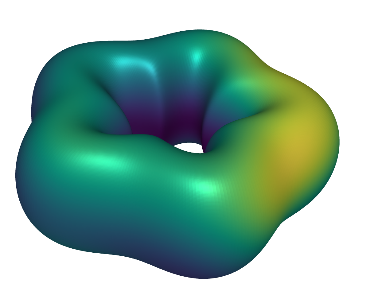
Figure 2: A wiggly torus geometry with parametrization $\bm{X}$ defined in Equation 6.1

Suppose that 6.3 is discretized using the Nyström method where the layer potentials are evaluated using the locally corrected quadrature methods discussed in [39]. We assume that the surface $\Gamma$ is given by the disjoint union of patches $\Gamma_{j}$, $\Gamma=\cup_{j=1}^{N_{\textrm{patches}}}\Gamma_{j}$, where each patch is parametrized by a non-degenerate chart $\bm{X}^{j}:T_{0}\to\Gamma_{j}$, with $T_{0}=\{(u,v):u>0,v>0,u+v\leq 1\}$ being the standard right simplex. We further assume that the charts $\bm{X}^{j}$, their derivative information, the density $\sigma|_{\Gamma_{j}}$ and the data $f|_{\Gamma_{j}}$ are discretized using order $p$ Vioreanu-Rokhlin nodes on $T_{0}$ [73, 39].

Let $n=N_{\textrm{patches}}p(p+1)/2$ be the total number of discretization points. Let $\varepsilon$ denote the tolerance used for computing the factorization (i.e. the tolerance requested in each interpolative decomposition performed). For a patch $\Gamma_{j}$, let $R_{j}$ denote the diameter of the patch and let ${\rm ppw}_{j}=R_{j}k/\pi$ denote the effective sampling rate on $\Gamma_{j}$ measured in points per wavelength. Let ${\rm ppw}_{{\rm min}}=\min_{j}{\rm ppw}_{j}$. Let $t_{f},t_{s}$ denote the factorization time and the solve time for computing FMM-LU factorization including quadrature corrections, respectively. Let $t_{q}$ denote the problem setup time which is dominated by the time taken to generate the quadrature corrections. Let $m_{f}$ denote the total memory required for storing the factorization in GB, and $S_{f}=n/t_{f},S_{s}=n/t_{s}$, and $S_{q}=n/t_{q}$ denote the corresponding speeds for the different tasks measured in points processed per second. Lastly, let $n_{0}$ denote the size of the system matrix inverted directly at the root level.

The fast direct solver was implemented in Matlab as a fork of github.com/victorminden/strong-skel, and relies on interfaces contained in the fmm3dbie library [39], freely available at github.com/fastalgorithms/fmm3dbie, and the FLAM library, freely available at github.com/klho/FLAM. The code used for the following experiments and timings can be obtained at github.com/fastalgorithms/strong-skel; a python implementation can be obtained at gitlab.com/fastalgorithms/adaptive-direct-h2. The experiments were run on a single core of a linux workstation with $192$ GB RAM. The current implementation is to demonstrate the accuracy of our approach and the complexity scaling with respect to the total number of discretization points for the various parts of the algorithm. An improved solver with better computational performance will be released soon.

6.1 Accuracy and convergence

To test the accuracy of the solver, suppose that the Dirichlet data is the potential due to a collection of $50$ random point sources located in the interior of $\Omega$ given by

$$f(\bm{x})=\sum_{j=1}^{50}q_{j}\frac{e^{ik|\bm{x}-\bm{x}_{j}|}}{|\bm{x}-\bm{x}_{j}|}\,.$$ (6.4)

In this setting, due to uniqueness, the exact solution in the exterior is given by the right hand side of the above expression evaluated at $\bm{x}\in\Omega^{c}$. Let $u_{\textrm{comp}}$ denote the numerically computed solution and let $\varepsilon_{a}$ denote the relative $L^{2}$ error at $50$ random target locations in the exterior denoted by $\bm{t}_{j}$, $j=1,2,\ldots 50$, given by

$$\varepsilon_{a}=\frac{\sqrt{\sum_{j=1}^{50}|u_{\textrm{comp}}(\bm{t}_{j})-u(\bm{t}_{j})|^{2}}}{\sqrt{\int_{\Gamma}|\sigma(\bm{x})|^{2}\,{\textrm{d}}a(\bm{x})}}\,.$$ (6.5)

In LABEL:tab:conv, we tabulate $t_{f}$, $t_{s}$, $t_{q}$ and $m_{f}$ for $p=6$ and $\varepsilon=5\times 10^{-7}$. The data are plotted in Figure LABEL:fig:graphs. For these experiments $k=0.97$ is chosen such that the torus is contained in a bounding box of size $1.2\lambda\times 1\lambda\times 0.5\lambda$, and $\varepsilon=5\times 10^{-7}$. We observe the expected linear scaling in $t_{q}$. However, for $t_{f},t_{s}$, and $m_{f}$ we observe sub-linear scaling due to the wavenumber being held fixed while $n$ is increased. The additional degrees of freedom introduced beyond a certain sampling in points per wavelength are more easily compressed. We observe the expected convergence rate of $\max{(h^{p-1},\varepsilon)}$ for $\varepsilon_{a}$, see Figure LABEL:fig:rates. This is consistent with the analysis in [6]. However, for $p=4$, and $N_{\textrm{patches}}=12800$, we also do not observe the expected order of convergence to the desired tolerance. This can be explained by the fact that the matrix entries corresponding to the far-interactions were generated using the underlying smooth quadrature as opposed to an appropriately oversampled smooth quadrature rule.

6.2 Oscillatory problems sampled at fixed points per wavelength

In this section, we perform the accuracy test as in Section 6.1 when the surface $\Gamma$ is sampled at a fixed number of points per wavelength. For these examples, $p=6$, $\varepsilon=5\times 10^{-7}$ and and $k/\sqrt{N_{\textrm{patches}}}$ is held fixed, so that ${\rm ppw}_{{\rm min}}\approx 10$. In LABEL:tab:freq, we tabulate $\varepsilon_{a}$, $n_{0}$, $t_{f}$, $t_{s}$, $t_{q}$, and $m_{f}$. The data are plotted in Figure LABEL:fig:graphsPPW. The error $\varepsilon_{a}$ remains nearly constant as $k,N_{\textrm{patches}}$ are increased since the surface is being sampled at nearly the same number of points per wavelength. The size, $n_{0}$, of the matrix at the root level grows like $n^{4/9}$. Since the factorization time will typically be dominated by the direct inversion at the root level as $k\to\infty$, the computational complexity of constructing the factorization will be $\mathcal{O}(n_{0}^{3})=\mathcal{O}(n^{4/3})$. In the current experiments, we still empirically observe an $\mathcal{O}(n)$ scaling in the factorization time as the frequency $k$ is not sufficiently large. The solve time, time for generating the locally corrected quadrature, and the memory used continue to scale as $\mathcal{O}(n)$ even in this setting. This can be explained by the fact that at the root level, the solve time and memory requirement grow as $\mathcal{O}(n_{0}^{2})=\mathcal{O}(n^{8/9})$, so the dominant cost for both the solve time and memory used is at the leaf level of the tree which is $\mathcal{O}(n)$. Since we are using locally-corrected quadratures, the number of near interactions that need to be precomputed are more or less constant as $k,N_{\textrm{patches}}\to\infty$, and thus the cost of computing them scales like $\mathcal{O}(n)$.

6.3 Computing an azimuthal sonar cross section

In this section, we compute the azimuthal monostatic sonar cross section for sound soft acoustic scatterers. As before, let $\Gamma$ denote the boundary of the scatterer whose interior is defined by $\Omega$. Let $\varphi$ denote the azimuthal angle in the $xy$ plane of the object, and let the azimuthal sonar cross section in the $\varphi$ direction be denoted by $R(\varphi)$. Furthermore, let $\mathcal{F}[u](\theta,\varphi)$ denote the far field pattern [29] of an outgoing solution $u$ to the Helmholtz equation:

$$u(\bm{x})=\frac{e^{{ikr}}}{r}\mathcal{F}[u](\theta,\varphi)+\mathcal{O}\left(\frac{1}{r^{2}}\right).$$ (6.6)

Next, let $u_{\varphi_{0}}$ denote the outgoing scattered field due an incident plane wave propagating in the direction $\bm{d}=(\cos(\varphi_{0}),\sin{(\varphi_{0})},0)$. Then, the monostatic cross section is given by

$$R(\varphi_{0})=\mathcal{F}[u_{\varphi_{0}}](0,-\varphi_{0}).$$ (6.7)

That is to say: the monostatic cross section is the reflected far field signature of the solution in the direction from which the incident plane wave originated.

As before, we represent the scattered field $u_{\varphi_{0}}$ using the combined field layer potential with unknown density $\sigma_{\varphi_{0}}$. Then, along the boundary $\Gamma$, the density $\sigma_{\varphi_{0}}(\bm{x})$ satisfies

$$\frac{1}{2}\sigma_{\varphi_{0}}(\bm{x})+\int_{\Gamma}K(\bm{x},\bm{y})\,\sigma_{\varphi_{0}}(\bm{y})\,da(\bm{y})=-e^{ik\bm{x}\cdot\bm{d}},$$ (6.8)

where the right hand side above is a plane wave propagating in the direction $\bm{d}$. It can then be shown that the azimuthal sonar cross section $R(\varphi_{0})$ can be expressed in terms of the solution $\sigma_{\varphi_{0}}$ as

$$R(\varphi_{0})=\frac{-ik}{4\pi}\int_{\Gamma}e^{-ik\bm{x}\cdot\bm{d}}\left(1-\bm{n}(\bm{x})\cdot\bm{d}\right)\sigma_{\varphi_{0}}(\bm{x})da(\bm{x}),$$ (6.9)

from which one can determine $\mathcal{F}[u_{\varphi_{0}}](0,-\varphi_{0})$.

In this example, we compute the azimuthal sonar cross section $R$ of a model airplane. The model airplane is $49.3$ wavelengths long with a wingspan of $49.2$ wavelengths and a vertical height of $13.7$ wavelengths. The plane also has several multiscale features: 2 antennae on the top of the fuselage, and 1 control unit on the bottom of the fuselage, see Figure LABEL:fig:a380. The ratio of the diameter of the largest triangle in the mesh to the smallest triangle is $\mathcal{O}(10^{3})$. The plane is discretized with $N_{\textrm{patches}}=125,344$ and $p=4$, resulting in $n=1,253,440$ discretization points.

In Figure LABEL:fig:a380, we plot the solution $\sigma_{\varphi_{0}}$ for $\varphi_{0}=\pi/2$, and in Figure LABEL:fig:rad_600, we plot the azimuthal sonar cross section computed at $1000$ equispaced azimuthal angles on $(0,2\pi]$. We also tested the accuracy of the factorization using the approach discussed in Section 6.1. To generate the validation boundary data, we use $120$ point sources located in the interior of the plane, and computed the accuracy of the numerical solution on a $101\times 101$ lattice of targets on a slice which cuts through the wing edge, whose normal is given by $(0,0,1)$. In this example, the requested precision was set to $\varepsilon=5\times 10^{-5}$, the factorization was computed on a $40$ core linux workstation with $768$ GB RAM, $t_{f}=17810s$, $t_{s}=32.2s$, $t_{q}=60.5s$, $m_{f}=459.5$GB, $n_{0}=17466$, and $\varepsilon_{a}=7.4\times 10^{-4}$.

7 Conclusions

Fast direct solvers for boundary integral equations on complex surfaces in three dimensions are just now beginning to be competitive with iterative techniques coupled with fast-multipole methods (or related acceleration techniques). A prototype for these schemes is the recursive skeletonization method introduced by Martinsson and Rokhlin [62], which motivated the subsequent hierarchical methods of [36, 49, 52, 60] and is related to the ${\cal H}$-matrix approach of [46, 48, 12]. These methods are more or less optimal in two dimensions but not in three dimensions because of the high-rank interaction between adjacent surface patches. The methods of [2, 10, 47, 58, 67, 31] which rely on strong skeletonization (strong admissibility, mosaic-skeletonization, ${\cal H}^{2}$-matrix compression, or the inverse FMM) avoid direct compression of these interactions, introducing more complex linear algebraic structures, with one approach described in the body of the present paper.

While we have focused on the FMM-LU solver as an extension of the RS-S method [67] while using high-order accurate quadratures at high precision, it should be noted that one can instead use a direct solver at low precision as a preconditioner for an iterative method. As noted in [67], this may be a more practical approach because of the reduction in memory requirements. At present, it seems as though the strong skeletonization framework leads to methods with both the best asymptotic scaling and the lowest memory requirements.

We have used the Helmholtz equation as our model problem in this work, and have limited our attention to the low or moderate frequency regime. For highly oscillatory problems, even well-separated blocks are of high rank and the interpolative decomposition does not lead to significant compression. Alternative compression techniques such as low rank directional compression [13, 11, 33] or butterfly compression [45, 57, 54] techniques are promising in this regime.

There are a number of open problems in this rapidly evolving field: a better understanding of the rank structure of the Schur complements that play a role in the recursive solver, optimization of proxy surface selection, extension to the high-frequency regime, and implementation on high-performance computing architectures. Finally, a number of integral equation formulations of scattering problems involve the composition of integral operators (see, for example, the regularized combined field equation for sound-hard scatterers [20, 39]). In that setting, the entries of the system matrix are not directly available in $\mathcal{O}(1)$ time. We are currently working on a number of these issues.

References

- [1] S. Ambikasaran and E. Darve. An Fast Direct Solver for Partial Hierarchically Semi-Separable Matrices. J. Sci. Comput., 57(3):477–501, 2013.
- [2] S. Ambikasaran and E. Darve. The Inverse Fast Multipole Method. arXiv preprint arXiv:1407.1572, 2014.
- [3] S. Ambikasaran, D. Foreman-Mackey, L. Greengard, D. W. Hogg, and M. O’Neil. Fast Direct Methods for Gaussian Processes. IEEE Trans. Pattern Anal. Mach. Intell., 38:252–265, 2016.
- [4] S. Ambikasaran, M. O’Neil, and K. R. Singh. Fast symmetric factorization of hierarchical matrices with applications. arXiv preprint arXiv:1405.0223, 2016.
- [5] K. E. Atkinson. The Numerical Solution of Integral Equations of the Second Kind. Cambridge University Press, New York, NY, 1997.
- [6] K. E. Atkinson and D. Chien. Piecewise polynomial collocation for boundary integral equations. SIAM J. Sci. Comput., 16:651–681, 1995.
- [7] R. Beatson and L. Greengard. A short course on fast multipole methods. In M. A. et al., editor, Wavelets, Multilevel Methods, and Elliptic PDEs, pages 1–37. Oxford University Press, 1997.
- [8] M. Bebendorf. Hierarchical LU decomposition-based preconditioners for BEM. Computing, 74(3):225–247, 2005.
- [9] S. Börm. 2lib package. http://www.h2lib.org/.
- [10] S. Börm. Efficient numerical methods for non-local operators: -matrix compression, algorithms and analysis, volume 14. European Mathematical Society, 2010.
- [11] S. Börm. Directional -matrix compression for high-frequency problems. Num. Lin. Alg. Appl., 24(6):e2112, 2017.
- [12] S. Börm, L. Grasedyck, and W. Hackbusch. Introduction to hierarchical matrices with applications. Eng. Anal. Bound Elem., 27(5):405–422, 2003.
- [13] S. Börm and J. M. Melenk. Approximation of the high-frequency Helmholtz kernel by nested directional interpolation: error analysis. Num. Math., 137(1):1–34, 2017.
- [14] S. Börm and K. Reimer. Efficient arithmetic operations for rank-structured matrices based on hierarchical low-rank updates. Comput. Vis. Sci., 16(6):247–258, 2013.
- [15] J. Bremer. On the Nyström discretization of integral equations on planar curves with corners. Appl. Comput. Harm. Anal., 32:45–64, 2012.
- [16] J. Bremer, A. Gillman, and P.-G. Martinsson. A high-order accelerated direct solver for integral equations on curved surfaces. BIT Num. Math., 55:367–397, 2015.
- [17] J. Bremer and Z. Gimbutas. A Nyström method for weakly singular integral operators on surfaces. J. Comput. Phys., 231:4885–4903, 2012.
- [18] J. Bremer and Z. Gimbutas. On the numerical evaluation of singular integrals of scattering theory. J. Comput. Phys., 251:327–343, 2013.
- [19] J. Bremer, Z. Gimbutas, and V. Rokhlin. A nonlinear optimization procedure for generalized Gaussian quadratures. SIAM J. Sci. Comput., 32(4):1761–1788, 2010.
- [20] O. Bruno, T. Elling, and C. Turc. Regularized integral equations and fast high-order solvers for sound-hard acoustic scattering problems. Int. J. Num. Meth. Engin., 91:1045–1072, 2012.
- [21] O. Bruno and E. Garza. A Chebyshev-based rectangular-polar integral solver for scattering by geometries described by non-overlapping patches. J. Comput. Phys., page 109740, 2020.
- [22] O. P. Bruno and L. A. Kunyansky. A fast, high-order algorithm for the solution of surface scattering problems: Basic implementation, tests, and applications. J. Comput. Phys., 169(1):80–110, 2001.
- [23] S. Chandrasekaran, M. Gu, and T. Pals. A fast ULV decomposition solver for hierarchically semiseparable representations. SIAM J. Matrix Anal. A., 28(3):603–622, 2006.
- [24] Y. Chen. A fast, direct algorithm for the Lippmann-Schwinger integral equation in two dimensions. Adv. Comput. Math., 16:175–190, 2002.
- [25] H. Cheng, W. Y. Crutchfield, Z. Gimbutas, L. Greengard, J. F. Ethridge, J. Huang, V. Rokhlin, N. Yarvin, and J. Zhao. A wideband fast multipole method for the Helmholtz equation in three dimensions. J. Comput. Phys., 216:300–325, 2006.
- [26] H. Cheng, Z. Gimbutas, P.-G. Martinsson, and V. Rokhlin. On the compression of low rank matrices. SIAM J. Sci. Comput., 26(4):1389–1404, 2005.
- [27] H. Cheng, L. Greengard, and V. Rokhlin. A fast adaptive multipole algorithm in three dimensions. J. Comput. Phys., 155(2):468–498, 1999.
- [28] D. Colton and R. Kress. Integral Equation Methods in Scattering Theory. John Wiley & Sons, Inc., 1983.
- [29] D. Colton and R. Kress. Inverse Acoustic and Electromagnetic Scattering Theory. Springer, New York, NY, 2012.
- [30] E. Corona, P.-G. Martinsson, and D. Zorin. An direct solver for integral equations on the plane. Appl. Comput. Harmon. A., 2014.
- [31] P. Coulier, H. Pouransari, and E. Darve. The inverse fast multipole method: Using a fast approximate direct solver as a preconditioner for dense linear systems. SIAM J. Sci. Comput., 39:A761–A796, 2017.
- [32] M. de Berg, O. Cheong, M. Kreveld, and M. Overmars. Computational Geometry: Algorithms and Applications. Springer, 2008.
- [33] B. Engquist and L. Ying. A fast directional algorithm for high frequency acoustic scattering in two dimensions. Commun. Math. Sci., 7:327–345, 2009.
- [34] S. Erichsen and S. A. Sauter. Efficient automatic quadrature in 3-D Galerkin BEM. Comput. Methods Appl. Mech. Engrg., 157:215–224, 1998.
- [35] A. Gillman, A. H. Barnett, and P.-G. Martinsson. A spectrally accurate direct solution technique for frequency-domain scattering problems with variable media. BIT Num. Math., 55:141–170, 2015.
- [36] A. Gillman, P. M. Young, and P.-G. Martinsson. A direct solver with complexity for integral equations on one-dimensional domains. Frontiers of Mathematics in China, 7(2):217–247, 2012.
- [37] A. Gopal and P.-G. Martinsson. An accelerated, high-order accurate direct solver for the Lippmann-Schwinger equation for acoustic scattering in the plane. Adv. Comput. Math., 48, 2022.
- [38] L. Greengard, D. Gueyffier, P.-G. Martinsson, and V. Rokhlin. Fast direct solvers for integral equations in complex three-dimensional domains. Acta Numerica, 18:243–275, 2009.
- [39] L. Greengard, M. O’Neil, M. Rachh, and F. Vico. Fast multipole methods for the evaluation of layer potentials with locally-corrected quadratures. J. Comput. Phys.: X, 10:100092, 2021.
- [40] L. Greengard and V. Rokhlin. A fast algorithm for particle simulations. J. Comput. Phys., 73(2):325–348, Dec. 1987.
- [41] L. Greengard and V. Rokhlin. The rapid evaluation of potential fields in three dimensions. In Vortex methods, pages 121–141. Springer, 1988.
- [42] L. Greengard and V. Rokhlin. On the numerical solution of two-point boundary value problems. Comm. Pure Appl. Math., 44:419–452, 1991.
- [43] L. Greengard and V. Rokhlin. A new version of the Fast Multipole Method for the Laplace equation in three dimensions. Acta Numerica, 6:229–269, 1997.
- [44] M. Gu and S. C. Eisenstat. Efficient algorithms for computing a strong rank-revealing QR factorization. SIAM J. Sci. Comput., 17(4):848–869, 1996.
- [45] H. Guo, Y. Liu, J. Hu, and E. Michielssen. A Butterfly-Based Direct Integral Equation Solver Using Hierarchical LU Factorization for Analyzing Scattering from Electrically Large Conducting Objects. IEEE Trans. Antennas Propag., 65(9):4742–4750, 2017.
- [46] W. Hackbusch. A sparse matrix arithmetic based on -matrices. Part I: Introduction to -matrices. Computing, 62(2):89–108, 1999.
- [47] W. Hackbusch, B. Khoromskij, and S. Sauter. On -matrices. In H.-J. Bungartz, et al. (eds.), Lectures on Applied Mathematics, pages 9–30. Springer-Verlag, Berlin Heidelberg, 2000.
- [48] W. Hackbusch and B. N. Khoromskij. A Sparse -Matrix Arithmetic. Computing, 64(1):21–47, 2000.
- [49] K. L. Ho and L. Greengard. A fast direct solver for structured linear systems by recursive skeletonization. SIAM J. Sci. Comput., 34:A2507–A2532, 2012.
- [50] K. L. Ho and L. Ying. Hierarchical interpolative factorization for elliptic operators: Integral equations. Comm. Pure Appl. Math., 69(7):1314–1353, 2016.
- [51] M. Jiang, Z. Rong, X. Yang, L. Lei, P. Li, Y. Chen, and J. Hu. Analysis of Electromagnetic Scattering From Homogeneous Penetrable Objects by a Strong Skeletonization-Based Fast Direct Solver. IEEE Trans. Antennas Propag., 70(8):6883–6892, 2022.
- [52] W. Y. Kong, J. Bremer, and V. Rokhlin. An adaptive fast direct solver for boundary integral equations in two dimensions. Appl. Comput. Harm. Anal., 31(3):346–369, 2011.
- [53] R. Kress. Linear Integral Equations. Springer, New York, NY, 2014.
- [54] Y. Li, H. Yang, E. Martin, K. L. Ho, and L. Ying. Butterfly factorization. Multiscale Model. Simul., 13(2):714–732, 2015.
- [55] E. Liberty, F. Woolfe, P.-G. Martinsson, V. Rokhlin, and M. Tygert. Randomized algorithms for the low-rank approximation of matrices. Proceedings of the National Academy of Sciences, 104(51):20167–20172, 2007.
- [56] Y. Liu. Fast Multipole Boundary Element Method: Theory and Applications in Engineering. Cambridge University Press, 2008.
- [57] Y. Liu, H. Guo, and E. Michielssen. A HSS Matrix-Inspired Butterfly-Based Direct Solver for Analyzing Scattering from Two-dimensional Objects. IEEE Antenn. Wirel. Pr., 16:1179–1183, 2016.
- [58] M. Ma and D. Jiao. Accuracy Directly Controlled Fast Direct Solution of General -Matrices and Its Application to Solving Electrodynamic Volume Integral Equations. IEEE Trans. Micro. Theory Tech., 66(1):35–48, 2018.
- [59] D. Malhotra, A. Cerfon, L.-M. Imbert-Gérard, and M. O’Neil. Taylor states in stellarators: A fast high-order boundary integral solver. J. Comput. Phys., 397:108791, 2019.
- [60] P. G. Martinsson. A fast randomized algorithm for computing a hierarchically semiseparable representation of a matrix. SIAM J. Matrix Anal. A., 32(4):1251–1274, 2011.
- [61] P.-G. Martinsson. Fast Direct Solvers for Elliptic PDEs. SIAM, 2019.
- [62] P.-G. Martinsson and V. Rokhlin. A fast direct solver for boundary integral equations in two dimensions. J. Comput. Phys, 205:1–23, 2005.
- [63] P.-G. Martinsson and V. Rokhlin. A fast direct solver for boundary integral equations in two dimensions. J. Comput. Phys., 205(1):1–23, 2005.
- [64] P.-G. Martinsson, V. Rokhlin, Y. Shkolnisky, and M. Tygert. ID: A software package for low-rank approximation of matrices via interpolative decompositions, Version 0.4. 0.4 edition, 2014.
- [65] V. Minden, A. Damle, K. L. Ho, and L. Ying. A technique for updating hierarchical skeletonization-based factorizations of integral operators. Multiscale Model. Simul., 14:42–64, 2016.
- [66] V. Minden, A. Damle, K. L. Ho, and L. Ying. Fast Spatial Gaussian Process Maximum Likelihood Estimation via Skeletonization Factorizations. Multiscale Model. Simul., 15(4):1584–1611, 2017.
- [67] V. Minden, K. L. Ho, A. Damle, and L. Ying. A recursive skeletonization factorization based on strong admissibility. Multiscale Model. Simul., 15(2):768–796, 2017.
- [68] V. Rokhlin. Rapid solution of integral equations of classical potential theory. J. Comput. Phys., 60(2):187–207, 1985.
- [69] M. Siegel and A.-K. Tornberg. A local target specific quadrature by expansion method for evaluation of layer potentials in 3d. J. Comput. Phys., 364:365–392, 2018.
- [70] S. Solovyev. Multifrontal Hierarchically Solver for 3D Discretized Elliptic Equations. In International Conference on Finite Difference Methods, pages 371–378. Springer, 2014.
- [71] P. Starr and V. Rokhlin. On the numerical solution of two-point boundary value problems II. Comm. Pure Appl. Math., 47:1117–1159, 1994.
- [72] D. A. Sushnikova and I. V. Oseledets. ”Compress and eliminate” solver for symmetric positive definite sparse matrices. SIAM J. Sci. Comput., 40(2):A1742–A1762, 2018.
- [73] B. Vioreanu and V. Rokhlin. Spectra of Multiplication Operators as a Numerical Tool. SIAM J. Sci. Comput., 36:A267–A288, 2014.
- [74] M. Wala and A. Klöckner. A fast algorithm for quadrature by expansion in three dimensions. J. Comput. Phys., 388:655–689, 2018.
- [75] M. Wala and A. Klöckner. Optimization of fast algorithms for global quadrature by expansion using target-specific expansions. J. Comput. Phys., 403, 2020.
- [76] B. Wu and P.-G. Martinsson. Corrected Trapezoidal Rules for Boundary Integral Equations in Three Dimensions. Num. Math., 149:1025–1071, 2021.
- [77] J. Xia, S. Chandrasekaran, M. Gu, and X. S. Li. Superfast multifrontal method for large structured linear systems of equations. SIAM J. Matrix Anal. A., 31(3):1382–1411, 2009.
- [78] J. Xia, S. Chandrasekaran, M. Gu, and X. S. Li. Fast algorithms for hierarchically semiseparable matrices. Numer. Linear Algebr., 17(6):953–976, 2010.
- [79] X. Xing and E. Chow. Interpolative Decomposition via Proxy Points for Kernel Matrices. SIAM J. Matrix Anal. Appl., 41(1):221–243, 2020.
- [80] X. Ye, J. Xia, and L. Ying. Analytical Low-Rank Compression via Proxy Point Selection. SIAM J. Matrix Anal. Appl., 41(3):1059–1085, 2020.
- [81] L. Ying, G. Biros, and D. Zorin. A high-order 3D boundary integral equation solver for elliptic PDEs in smooth domains. J. Comput. Phys., 219(1):247–275, 2006.