1 Introduction

We consider the linear regression with a structural break, following the notations of Bai (1997):

$$y_{t}=\begin{cases}w_{t}^{\prime}\alpha+z_{t}^{\prime}\delta_{1}+\epsilon_{t},&\text{for}\ t=1,\ldots,\left\lfloor\tau T\right\rfloor\\ w_{t}^{\prime}\alpha+z_{t}^{\prime}\delta_{2}+\epsilon_{t},&\text{for}\ t=\left\lfloor\tau T\right\rfloor+1,\ldots,T,\end{cases}$$ (1)

where $w_{t}$ and $z_{t}$ are $d_{w}\times 1$ and $d_{z}\times 1$ vectors of covariates, and the random variable $\epsilon_{t}$ is a regression error. $\left\lfloor a\right\rfloor$ is the largest integer that is strictly smaller than $a$. The relationship between the outcome $y_{t}$ and the covariate $z_{t}$, measured by $\delta$’s, changes across regimes, which are defined by the break location parameter $\tau\in(0,1)$. There can be another set of covariates $w_{t}$ whose relationship with $y_{t}$, measured by $\alpha$, stays unchanged across the regimes. The unknown parameters include the break location $\tau$ as well as the slope parameters $\gamma=(\alpha,\delta_{1},\delta_{2})$. The focus of the current study is on inference about the slope parameter $\gamma$.

1.1 The classic literature

In the literature, the conventional least-squares estimators $\left(\hat{\tau}_{LS},\hat{\gamma}_{LS}\right)$ for $\left(\tau,\gamma\right)$ are computed as follows: for each candidate $\tau$, compute the sum of squared residuals of the regression and denote the minimizing choice by $\hat{\tau}_{LS}$. Plug in the value $\tau=\hat{\tau}_{LS}$ in the model and define $\hat{\gamma}_{LS}=\hat{\gamma}(\hat{\tau}_{LS})$, where $\hat{\gamma}({\tau})$ is the usual OLS estimator of $\gamma$ assuming the break location $\tau$. Bai (1997) assumes that the true jump size $\delta_{0}$ is either fixed or shrinks to zero as $T\to\infty$, but at a rate slower than $\sqrt{T}\to\infty$. Bai shows that $\hat{\tau}_{LS}$ converges at the rate $T^{-1}$ in the former case and, in the latter case, finds an asymptotic distribution of $\hat{\tau}_{LS}$ that can be used for constructing confidence intervals for $\tau$. In both cases, Bai proves that the asymptotic distribution of $\hat{\gamma}_{LS}$ is the same as that of $\hat{\gamma}(\tau_{0})$, where $\tau_{0}$ is the true value of $\tau$. This means that one can ignore the very problem of unknown $\tau$ when making inference on $\gamma$.

Figure 1 displays finite-sample distributions of $\hat{\tau}_{LS}$ (blue solid curves) which are produced based on 1,000 repeated experiments on the following model $y_{t}=\delta_{0}1\left(t>\left\lfloor\tau_{0}T\right\rfloor\right)+\epsilon_{t}$. Note that despite the $T$-consistency, $\hat{\tau}_{LS}$ displays significant variation, especially when the true break size $\delta_{0}$ is small. In practice, the conventional approach to inference on the slope parameters $\gamma$ would ignore this uncertainty, neglecting all possible values of $\tau$ other than $\hat{\tau}_{LS}$. As a consequence, the corresponding confidence intervals on $\gamma$ tend to undercover since it might not be the case that $\hat{\tau}_{LS}=\tau_{0}$ in a given sample (See our simulation in Section 5).

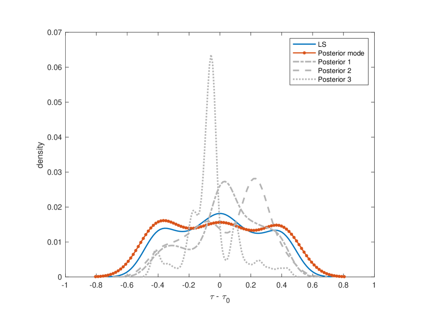
(a) $\delta_{0}=0.25$

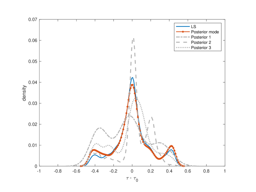
(b) $\delta_{0}=0.5$

Figure 1: Finite-sample distribution of $\hat{\tau}_{LS}$ (blue solid curve) based on the model $y_{t}=\delta_{0}1\left(t>\left\lfloor\tau_{0}T\right\rfloor\right)+\epsilon_{t}$, $\epsilon_{t}\sim\text{i.i.d.}N(0,1),\tau_{0}=0.5,T=100$, with 1,000 repeated experiments. The horizontal axis is $\tau-\tau_{0}$. We also show finite-sample distribution of the posterior mode of $\tau$ (red solid curve with small circles). In addition, we randomly chose 3 data realizations out of the 1,000 repetitions to plot posterior densities of $\tau$ in gray dashed curves (hence each of them represents a realization of one data set).

1.2 Bayesian perspective

For a Bayesian, this non-standard estimation problem can be dealt with by placing prior on both $\tau$ and $\gamma$ and by computing corresponding posterior probabilities. The uncertainty of $\tau$ will be automatically reflected on the marginal posterior probability of $\gamma$. This is because the posterior distribution of $\gamma$ given the data $\bm{D}_{T}$ can be written as a mixture where the weights correspond to the marginal posterior density $\pi_{T}(\tau)$ for $\tau$:

$$p\left(\gamma|\bm{D}_{T}\right)=\int_{0}^{1}p\left(\gamma|\tau,\bm{D}_{T}\right)\pi_{T}(\tau)d\tau,$$ (2)

where $p\left(\gamma|\tau,\bm{D}_{T}\right)$ is the posterior conditional distribution of $\gamma$ given $\tau$. The posterior density $\pi_{T}(\tau)$ reflects the uncertainty of $\tau$ given the data set. Figure 1 shows three realizations of $\pi_{T}(\tau)$ (gray dashed curves) which are randomly chosen out of the 1,000 repetitions. Compared to the conventional approach, the key difference is that the Bayesian approach (2) incorporates all possibilities of $\tau$ (not just $\hat{\tau}_{LS}$) and weights them according to the posterior density. As we see in simulation studies, this results in longer lengths of Bayesian credible intervals of $\gamma$ compared to the conventional counterparts. Consequently, the credible intervals tend to avoid undercoverage. See Section 5 for further discussion. Note that, unlike conventional frequentist methods, Bayesian inference has a valid interpretation even in finite samples as it does not rely on asymptotic theory.

In this study, we examine the asymptotic behavior of Bayesian estimation of the considered model under the fixed jump size framework. Specifically, we prove a Bernstein-von Mises type theorem for the slope parameters $\gamma$ which validates a frequentist interpretation of Bayesian credible regions. A Bayesian researcher can invoke our theorem to convey statistical results to frequentist researchers. A frequentist researcher could look at the credible interval of $\gamma$ to check robustness with respect to the uncertainty of the break location. Such sensitivity analysis is reasonable as our result guarantees the credible interval to converge to the conventional confidence interval. We first establish theoretical results under normal likelihood and natural conjugate prior. We further extend the results to non-conjugate priors using Laplace approximations.

The literature on the theoretical properties of Bayesian approaches in non-regular models such as (1) is very scarce despite their popularity in applications. To our knowledge, frequentist properties of the Bayesian approach for linear regression models with structural breaks have not been studied in the literature. Ghosal  Samanta (1995) consider a general non-regular estimation problem from a Bayesian perspective and establish conditions under which the Bernstein-von Mises theorem holds for the regular part of the parameter. However, their assumptions are difficult to verify in regard to our model in consideration.

Recently, Casini  Perron (2020) propose a generalized Laplace estimator of the break location $\tau$ which is defined by an integration rather than an optimization. Their approach provides a better approximation about the uncertainty in $\tau$ than the conventional method. Although our focus of the current paper is on inference about the slope coefficients $\gamma$ and not $\tau$, our Bayesian approach toward inference shares the same spirit; any statement about $\gamma$ is expressed as a weighted average (2) over the marginal posterior density of $\tau$.

The paper is organized as follows. Section 2 introduces the model and lists a set of assumptions. Section 3 introduces a Bayesian approach based on normal likelihood and conjugate prior. The section then establishes frequentist properties of the approach. Section 4 extends the results to non-conjugate priors. Section 5 presents simulation evidence to assess the adequacy of the asymptotic theory and to illustrate that conventional confidence intervals on the slope parameters tend to undercover. Section 6 reports an empirical application to the stock return prediction model of Paye  Timmermann (2006). Section 7 concludes the paper. The mathematical proofs and derivations are listed in the Appendix. Additional tables are provided in the online appendix.

2 The model and data generating process

2.1 The model

Using the reparametrization $x_{t}=(w_{t}^{\prime},z_{t}^{\prime})^{\prime}$, $\beta=(\alpha^{\prime},\delta_{1}^{\prime})^{\prime}$, and $\delta=\delta_{2}-\delta_{1}$, the equations (1) can be rewritten as

$$y_{t}=\begin{cases}x_{t}^{\prime}\beta+\epsilon_{t},&\text{for}\ i=1,\ldots,\left\lfloor\tau T\right\rfloor\\ x_{t}^{\prime}\beta+z_{t}^{\prime}\delta+\epsilon_{t},&\text{for}\ i=\left\lfloor\tau T\right\rfloor+1,\ldots,T.\end{cases}$$ (3)

Note that $z_{t}$ is a subvector of $x_{t}$. More generally, let $z_{t}=R^{\prime}x_{t}$, where $R$ is a $d_{x}\times d_{z}$ known matrix with full column rank and hence $z_{t}$ is defined as a linear transformation of $x_{t}$. For $R=(0_{d_{z}\times d_{w}},I_{d_{z}})^{\prime}$, we obtain model (3). For $R=I_{d_{x}}$, a pure change model is obtained. To rewrite the model in matrix form, we introduce further notations. Define $Y=(y_{1},\ldots,y_{T})^{\prime}$, $\epsilon=(\epsilon_{1},\ldots,\epsilon_{T})^{\prime}$, $X=(x_{1},\ldots,x_{T})^{\prime}$, $X_{1\tau}=(x_{1},\ldots,x_{\left\lfloor\tau T\right\rfloor},0,\ldots,0)^{\prime}$, $X_{2\tau}=(0,\ldots,0,x_{\left\lfloor\tau T\right\rfloor+1},\ldots,x_{T})^{\prime}$. Define $Z,Z_{1\tau}$, and $Z_{2\tau}$ similarly. Then, $Z=XR$, $Z_{1\tau}=X_{1\tau}R$, and $Z_{2\tau}=X_{2\tau}R$. Now, the equations (3) can be written as

$$Y=X\beta+Z_{2\tau}\delta+\epsilon=\chi_{\tau}\gamma+\epsilon,$$ (4)

where $\chi_{\tau}=(X,Z_{2\tau})$ and $\gamma=(\beta^{\prime},\delta^{\prime})^{\prime}$. $S_{T}(\tau)$ denotes the sum of squared residuals of the regression (4) given $\tau$. Let $\mathcal{H}\subset(0,1)$ be the space of the break locations. The least-squares estimator of $\tau$ is defined as

$$\hat{\tau}_{LS}=\operatorname*{arg\,min}_{\tau\in\mathcal{H}}S_{T}(\tau),$$ (5)

and the least-squares estimator for the slope coefficients $\gamma=(\beta^{\prime},\delta^{\prime})^{\prime}$ is

$$\hat{\gamma}_{LS}=\hat{\gamma}(\hat{\tau}_{LS}),$$ (6)

where $\hat{\gamma}(\tau)$ denotes the usual OLS estimator given the value of $\tau$.

2.2 Data generating process

The data are assumed to include $T$ observations on a response and a vector of covariates: $\bm{D}_{T}=(\bm{Y}_{T},\bm{X}_{T})=(y_{1},\ldots,y_{T},x_{1},\ldots,x_{T})$ where $y_{t}\in\mathbb{R}$ and $x_{t}\in\mathcal{X}\subset\mathbb{R}^{d_{x}}$, $t=1,...,T$. $\mathcal{X}$ is assumed to be a convex and bounded set. Conditional on $\bm{X}_{T}$, the response is generated according to model (4) with the true parameters $(\gamma_{0}^{\prime},\sigma_{0}^{2},\tau_{0})^{\prime}$. We use $\theta=(\gamma^{\prime},\sigma^{2})^{\prime}$ to denote the regression parameters. We make the following assumptions about the true data-generating-process (DGP):

Assumption 1.

1. $\delta_{0}\neq 0$.

2. $\epsilon_{t}$ is i.i.d. with $E(\epsilon_{t}|x_{t})=0$, $E(\epsilon_{t}^{2}|x_{t})=\sigma_{0}^{2}$, where $\sigma_{0}^{2}$ is unknown to the econometrician.

3. $\Sigma_{X}=E[x_{t}x_{t}^{\prime}]=\operatorname*{plim}\frac{1}{T}\sum_{t=1}^{T}x_{t}x_{t}^{\prime}$ exists and is positive definite.

4. For all $\tau_{1},\tau_{2}\in(0,1)$ with $\tau_{1}<\tau_{2}$, $\frac{1}{T}\sum_{\left\lfloor\tau_{1}T\right\rfloor+1}^{\left\lfloor\tau_{2}T\right\rfloor}x_{t}\epsilon_{t}=O_{p}(T^{-1/2})$ and $\frac{1}{T}\sum_{\left\lfloor\tau_{1}T\right\rfloor+1}^{\left\lfloor\tau_{2}T\right\rfloor}x_{t}x_{t}^{\prime}=(\tau_{2}-\tau_{1})\Sigma_{X}+O_{p}(T^{-1/2})$

Under the above assumptions, the classical theoretical results apply. Bai (1997) shows that the convergence rate of $\hat{\tau}_{LS}$ is $T^{-1}$ if $\delta_{0}$ is fixed with respect to the sample size:

$$\hat{\tau}_{LS}=\tau_{0}+O_{p}(T^{-1}),$$

and that the least-squares estimator for $\gamma$ is asymptotically normal with the asymptotic covariance matrix being the same as if $\tau_{0}$ is known:

$$\sqrt{T}\left(\hat{\gamma}_{LS}-\gamma_{0}\right)\overset{d}{\to}N_{(d_{x}+d_{z})}(0,\sigma_{0}^{2}V^{-1}),$$ (7)

where

$$V=\operatorname*{plim}T^{-1}\begin{pmatrix}\sum_{t=1}^{T}x_{t}x_{t}^{\prime}&\sum_{t=\left\lfloor\tau_{0}T\right\rfloor+1}^{T}x_{t}z_{t}^{\prime}\\ \sum_{t=\left\lfloor\tau_{0}T\right\rfloor+1}^{T}z_{t}x_{t}^{\prime}&\sum_{t=\left\lfloor\tau_{0}T\right\rfloor+1}^{T}z_{t}z_{t}^{\prime}\end{pmatrix}=\operatorname*{plim}T^{-1}\chi_{\tau_{0}}^{\prime}\chi_{\tau_{0}}.$$

This means that $\tau$ can be treated as known for the purpose of inference about $\gamma$. In other words, the uncertainty of the break location is essentially ignored, and thus the confidence interval for $\gamma$ tends to undercover (see Section 5 for simulation).

There are several comments on Assumption 1. In threshold regression models (see Hansen, 2000), the threshold variable is often one of the regressors. In this case, sorting the threshold variable leads to a trend in the regressors, which requires an alternative approach for the asymptotic analysis. We do not consider the case with one of the regressors being the threshold variable in this paper. In addition, we require the regression errors to be i.i.d. with variance $\sigma^{2}$. Adding more flexibility such as heteroscedasticity and serial correlation would be an important future direction.

3 A Bayesian approach under normal likelihood and conjugate prior

The distribution of covariates is assumed to be ancillary and it is not modeled. Throughout this paper, we assume the normal likelihood function

$$p(\bm{Y}_{T}|\bm{X}_{T},\theta,\tau)=\prod_{t=1}^{T}\frac{1}{\sqrt{2\pi\sigma^{2}}}\exp\left(-\frac{\left(y_{t}-\chi_{\tau,t}^{\prime}\gamma\right)^{2}}{2\sigma^{2}}\right),$$ (8)

where $\chi_{\tau,t}^{\prime}$ is the $t$th row of the matrix $\chi_{\tau}$. Note that the normality is not assumed for the true DGP, so the model can be mis-specified.

The break location $\tau$ and the regression parameters $\theta$ are independent a-priori and the prior on $\theta$ is the natural conjugate prior. That is, $\pi\left(\gamma,\sigma^{2},\tau\right)=\pi(\gamma|\sigma^{2})\pi(\sigma^{2})\pi(\tau)$ where the prior on $\gamma$ conditional on $\sigma^{2}$ is normal $N_{(d_{x}+d_{z})}(\underline{\mu},\sigma^{2}\underline{H}^{-1})$ and the prior on $\sigma^{2}$ is inverse-gamma $InvGamma(\underline{a},\underline{b})$. Note that by taking $\underline{H}\to 0$, $\underline{a}\to-(d_{x}+d_{z})/2$, and $\underline{b}\to 0$, we have the uninformative improper prior $\pi\left(\gamma,\sigma^{2}\right)\propto\sigma^{-2}$ as a special case. The prior on $\tau$ can be of any form as long as it is positive at $\tau_{0}$, and $\pi(\tau)$ is finite for all $\tau\in\mathcal{H}$.

The conjugate prior is a popular choice in the Bayesian estimation of linear regression models. Our restriction on the prior for the break location $\tau$ is very mild. For example, the uniform distribution on $\mathcal{H}$ satisfies the requirement. Recently, Baek (2021) investigates the same model (1). As the distribution of $\hat{\tau}_{LS}$ might exhibit tri-modality for small jumps, Baek proposes a new point estimator for $\tau$ based on a modified objective function. The proposed modification can be regarded as equivalent to specifying a certain type of prior for $\tau$ and indeed such prior satisfies our restriction.

Under the normal likelihood function and the prior defined above, the posterior distributions are

$$\pi(\tau|\bm{D}_{T}) \propto\left[\det\left(\bar{H}_{\tau}\right)\right]^{-0.5}\bar{b}_{\tau}^{-\bar{a}}\times\pi(\tau),$$ (9)

$$\gamma\big{|}\tau,\bm{D}_{T} \sim t_{(d_{x}+d_{z})}\left(2\bar{a},\bar{\mu}_{\tau},(\bar{b}_{\tau}/\bar{a})\bar{H}_{\tau}^{-1}\right),$$ (10)

$$\sigma^{2}|\tau,\bm{D}_{T} \sim InvGamma\left(\bar{a},\bar{b}_{\tau}\right),$$ (11)

where $\bar{H}_{\tau}=\underline{H}+\chi_{\tau}^{\prime}\chi_{\tau}$, $\bar{\mu}_{\tau}=\bar{H}_{\tau}^{-1}\left[\underline{H}\underline{\mu}+\chi_{\tau}^{\prime}Y\right]$, $\bar{b}_{\tau}=\underline{b}+0.5\left[\underline{\mu}^{\prime}\underline{H}\underline{\mu}+Y^{\prime}Y-\bar{\mu}_{\tau}^{\prime}\bar{H}_{\tau}\bar{\mu}_{\tau}\right]$, and $\bar{a}=\underline{a}+T/2$, and $t_{k}(v,\mu,\Sigma)$ is the $k$-dimensional t-distribution with $v$ degrees of freedom, a location vector $\mu\in\mathbb{R}^{k}$, and a $k\times k$ shape matrix $\Sigma$. See Appendix C for the derivation.

Due to the availability of the closed-forms for the conditional posteriors given $\tau$, the posterior sampling is simple and fast. One can first draw $\tau_{(1)},\ldots,\tau_{(S)}$ from the marginal posterior of $\tau$ as in (9) via, for example, the Metropolis-Hastings algorithm, where $S$ is the number of posterior draws. For each $\tau_{(s)}$, one can sample posterior draws of $\sigma^{2}_{(s)}$ from the posterior conditional on $\tau=\tau_{(s)}$, namely (11). Conditional on $\tau$ and $\sigma^{2}$, one can draw $\gamma$ from $p(\gamma|\sigma^{2},\tau,\bm{D}_{T})$. For example, a laptop with a 2.2GHz processor and 8GB RAM takes about 4.1 seconds to draw 10,000 posterior draws in an empirical example in Section 6 that has ten slope coefficients in total.

3.1 Asymptotic theory

We investigate the asymptotic behavior of the Bayesian method under the normal likelihood and the conjugate prior defined above. We do so in two steps. Section 3.1.1 shows that the marginal posterior of the break location $\tau$ contracts to the true value $\tau_{0}$ at the rate of $T^{-1}$, the same rate at which the least-squares estimator $\hat{\tau}_{LS}$ converges. The proof is based on studying the behavior of the log ratio of the marginal posterior densities of $\tau$. In addition, we establish the limiting distribution of the posterior mode of $\tau$. Section 3.1.2 establishes a Bernstein-von Mises type theorem for the regression slope coefficients $\gamma$. The proof is based on the $T$-consistency of the marginal posterior of $\tau$ and the fact that the conditional posterior for $\sqrt{T}\left(\gamma-\hat{\gamma}_{LS}\right)$ given $\tau$ is asymptotically normal. Proofs of the theorems can be found in Appendix A.

3.1.1 Marginal posterior of $\tau$

An intermediate step for proving the Bernstein-von Mises theorem is the marginal posterior consistency of $\tau$ at rate $T^{-1}$. Marginal posteriors have not been studied extensively or systematically in the literature. Here, we directly analyze the form of the marginal posterior of $\tau$. Let $L_{T}(\tau)$ be the marginal likelihood conditional on $\tau$, that is

$$L_{T}(\tau)=\int p(\bm{Y}_{T}|\bm{X}_{T},\theta,\tau)\pi(\theta,\tau)d\theta,$$

which is available up to a multiplicative constant under the normal likelihood and the conjugate prior as can be seen in (9). The marginal posterior density $\pi_{T}(\tau)$ of $\tau$ is defined as

$$\pi_{T}(\tau)=\frac{L_{T}(\tau)}{\int L_{T}(\tau)d\tau}.$$

The following theorem establishes the first step for proving the Bernstein-von Mises theorem, the $T$-consistency of the marginal posterior of $\tau$. It states that the posterior mass outside of a ball around $\tau_{0}$ with radius proportional to $T^{-1}$ will be asymptotically negligible.

Theorem 1 (Marginal posterior consistency of $\tau$ at rate $T^{-1}$).

Suppose Assumption 1 holds. Then, under the normal likelihood and the conjugate prior described above, $\forall\eta>0,\epsilon>0$, $\exists M>0$ and $k>0$ such that $T\geq k\implies$

$$P_{\theta_{0},\tau_{0}}\left(\int_{B^{c}_{M/T}(\tau_{0})}\pi_{T}(\tau)d\tau<\eta\right)>1-\epsilon,$$

where for any constant $d>0$, $B^{c}_{d}(\tau_{0})$ denotes the set difference $\mathcal{H}\setminus(\tau_{0}-d,\tau_{0}+d)$.

The proof of Theorem 1 is built on some intermediate steps, Propositions 1-4. It can be shown that $\int_{B^{c}_{M/T}(\tau_{0})}\pi_{T}(\tau)d\tau$ is bounded by the product of $\int_{B^{c}_{M/T}(\tau_{0})}\frac{L_{T}(\tau)}{L_{T}(\tau_{0})}d\tau$ and the inverse of $\int_{B^{c}_{M_{0}/T}(\tau_{0})}\frac{L_{T}(\tau^{\prime})}{L_{T}(\tau_{0})}d\tau^{\prime}$ for each $T$ and for any $M_{0}>0$. Proposition 1 shows that under the normal likelihood and the conjugate prior, due to the availability of the marginal likelihood conditional on $\tau$ up to a normalization constant as in (9), studying the log marginal likelihood ratio boils down to comparing the sum of squared residuals $S_{T}(\tau)$. Proposition 2 establishes the probability limit of $T^{-1}S_{T}(\tau)$, for which we show examples in Figure 2. We then show that the limit of $T^{-1}S_{T}(\tau)$ achieves a unique minimum at $\tau_{0}$ (Proposition 3), and study the modulus of continuity of an appropriate empirical process (Proposition 4) in order to derive bounds. The detail of the proof of Theorem 1 can be found in Appendix A.1.

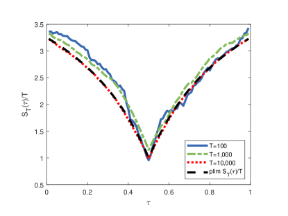
Figure 2: Example of $T^{-1}S_{T}(\tau)$ with $T=100$ (solid, blue), $T=1,000$ (dash-dotted, green), and $T=10,000$ (dotted, red) and $\operatorname*{plim}T^{-1}S_{T}(\tau)$ (dashed, black)

The Bayesian counterpart of the least-squares estimator $\hat{\tau}_{LS}$ would be the posterior mode:

$$\hat{\tau}_{Bayes}=\operatorname*{arg\,max}_{\tau\in\mathcal{H}}\pi_{T}(\tau).$$

Bai (1997) shows that $\operatorname*{arg\,max}_{m}W^{*}(m)$ is the asymptotic distribution of $\hat{\tau}_{LS}$ . A consequence of the proof of Theorem 1 is that $\hat{\tau}_{Bayes}$ converges to the same limiting distribution. See Appendix A.2 for a proof.

Corollary 1 (Limiting distribution of the posterior mode of $\tau$).

Suppose Assumption 1 holds. Then, under the normal likelihood and the conjugate prior described above,

$$\left\lfloor T\left(\hat{\tau}_{Bayes}-\tau_{0}\right)\right\rfloor\overset{d}{\to}\operatorname*{arg\,max}_{m}W^{*}(m).$$

3.1.2 Bernstein-von Mises Theorem for $\gamma$

The marginal posterior of $\gamma$ is a mixture with weights corresponding to the marginal posterior density $\pi_{T}(\tau)$. Furthermore, due to Theorem 1, we can focus our attention on the values of $\tau$ in a $T^{-1}$ neighborhood of $\tau_{0}$:

$$\int p(\gamma|\tau,\bm{D}_{T})\pi_{T}(\tau)d\tau=\int_{B_{M/T}(\tau_{0})}p(\gamma|\tau,\bm{D}_{T})\pi_{T}(\tau)d\tau+o_{p}(1).$$

We are now ready to establish the Bernstein-von Mises type result.

Theorem 2 (Bernstein-von Mises theorem for the slope coefficients).

Suppose Assumption 1 holds. Then, under the normal likelihood and the conjugate prior described above,

$$d_{TV}\left(\pi\left[\begin{matrix}\sqrt{T}\left(\gamma-\hat{\gamma}_{LS}\right)\end{matrix}\bigg{|}\bm{D}_{T}\right],N_{(d_{x}+d_{z})}\left(0,\sigma^{2}_{0}V^{-1}\right)\right)\to 0,$$

in $P_{\theta_{0},\tau_{0}}-probability$ where $d_{TV}$ is the total variation distance.

The proof of Theorem 2 exploits the fact that the conditional posterior for $\sqrt{T}\left(\gamma-\hat{\gamma}_{LS}\right)$ given $\tau$ is asymptotically normal, which is close to the asymptotic distribution of $\hat{\gamma}_{LS}$ when $\tau$ is close to $\tau_{0}$. A bound on the Kullback–Leibler (KL) divergence between two normal densities together with the $T$-consistency is used to make the argument precise. The proof is presented in Appendix A.3.

4 An extension to non-conjugate priors

The previous section establishes the asymptotic properties of the posterior distributions under the conjugate prior. A natural question is whether these results can be extended to other priors. For example, an independent prior between the slope coefficients $\gamma$ and the error variance $\sigma^{2}$, e.g., $\pi(\gamma,\sigma^{2})=\pi(\gamma)\pi(\sigma^{2})$ with $\gamma\sim N_{(d_{x}+d_{z})}(\underline{\mu},\underline{\Sigma})$ and $\sigma^{2}\sim InvGamma(\underline{a},\underline{b})$, is a popular choice for the Bayesian estimation of regression models in practice. Under the normal likelihood and the conjugate prior, the analytical expressions of the marginal posterior of $\tau$ up to a normalization constant (9) and the conditional posterior of $\gamma$ given $\tau$ (10) facilitate the theoretical analysis. They are not available, for instance, under the independent prior mentioned above. In this section, we extend the theoretical results by keeping the normal likelihood (8) but without requiring the conjugate prior on $\theta$. In order to study the asymptotic behavior of the posterior distributions without having their closed-form expressions, we employ Laplace approximation type results in Hong  Preston (2012). To do so, we make an additional assumption as shown below. Let $\hat{\theta}(\tau)$ be the maximum likelihood estimator of $\theta$ conditional on $\tau\in\mathcal{H}$, i.e., $\hat{\theta}(\tau)=\arg\sup_{\theta\in\Theta}\log p(\bm{Y}_{T}|\bm{X}_{T},\theta,\tau)$. Denote by $\theta^{*}(\tau)$ the corresponding pseudo true parameter value that minimizes the KL divergence between the model $p(\bm{Y}_{T}|\bm{X}_{T},\theta,\tau)$ and the DGP.

Assumption 2.

1. There is a compact convex subset $\Theta$ of $\mathbb{R}^{d_{x}+d_{z}+1}$ such that $\theta^{*}(\tau)\in int\left(\Theta\right)$ for all $\tau\in\mathcal{H}$.

2. The prior $\pi(\theta,\tau)$ is supported on $\Theta\times\mathcal{H}$. It is continuous in $\theta$ and bounded away from 0 and $\infty$ around $\left(\theta^{*}(\tau),\tau\right)$ for all $\tau\in\mathcal{H}$.

Under the normal likelihood and Assumption 1, together with Assumption 2, we can invoke the Laplace approximation results of Hong  Preston (2012). Note that, under the normal likelihood and Assumption 1, $\theta^{*}(\tau)$ exists and is a function of parameters in the DGP. In this section, we no longer assume the natural conjugate prior on $\theta$. For instance, the independent prior $\pi(\gamma,\sigma^{2},\tau)=\pi(\gamma)\pi(\sigma^{2})\pi(\tau)$ mentioned above satisfies the conditions in (ii) of Assumption 2 as long as they are truncated on $\Theta$ and $\pi(\tau)$ is positive and finite at all $\tau$.

Theorem 3 below establishes the $T$-consistency of the marginal posterior of $\tau$ under this prior and the additional assumption.

Theorem 3 (Marginal posterior consistency of $\tau$ at rate $T^{-1}$, non-conjugate priors).

Suppose Assumptions 1 and 2 hold. Then, under the normal likelihood, $\forall\eta>0,\epsilon>0$, $\exists M>0$ and $k>0$ such that $T\geq k\implies$

$$P_{\theta_{0},\tau_{0}}\left(\int_{B^{c}_{M/T}(\tau_{0})}\pi_{T}(\tau)d\tau<\eta\right)>1-\epsilon,$$

where for any constant $d>0$, $B^{c}_{d}(\tau_{0})$ denotes the set difference $\mathcal{H}\setminus(\tau_{0}-d,\tau_{0}+d)$.

Recall that while proving the $T$-consistency under the conjugate prior (i.e., Theorem 1), we utilize the closed-form expression of the marginal posterior of $\tau$ up to a multiplicative constant (9) in order to study the behavior of the marginal likelihood ratio conditional on $\tau$. Under non-conjugate priors, such expression is not available in general. For this reason, we invoke a Laplace approximation to investigate the quantity $\int p(\bm{Y}_{T}|\bm{X}_{T},\theta,\tau)\pi(\theta,\tau)d\theta$ to prove Theorem 3. See Appendix A.4 for the detail.

As in the previous section, an implication of the $T$-consistency of the marginal posterior of $\tau$ is that the posterior mode converges to the limiting distribution of $\hat{\tau}_{LS}$. Proof is in Appendix A.5.

Corollary 2 (Limiting distribution of the posterior mode of $\tau$, non-conjugate priors).

Suppose Assumptions 1 and 2 hold. Then, under the normal likelihood,

$$\left\lfloor T\left(\hat{\tau}_{Bayes}-\tau_{0}\right)\right\rfloor\overset{d}{\to}\operatorname*{arg\,max}_{m}W^{*}(m),$$

where the stochastic process $W^{*}(m)$ is defined in Section 3.1.1.

Theorem 4 establishes our main theoretical result, the Bernstein-von Mises theorem for $\gamma$, under the prior defined in Assumption 2 (ii).

Theorem 4 (Bernstein-von Mises theorem for the slope coefficients, non-conjugate priors).

Suppose Assumptions 1 and 2 hold. Then, under the normal likelihood,

$$d_{TV}\left(\pi\left[\begin{matrix}\sqrt{T}\left(\gamma-\hat{\gamma}_{LS}\right)\end{matrix}\bigg{|}\bm{D}_{T}\right],N_{(d_{x}+d_{z})}\left(0,\sigma^{2}_{0}V^{-1}\right)\right)\to 0,$$

in $P_{\theta_{0},\tau_{0}}-probability$ where $d_{TV}$ is the total variation distance.

When proving the corresponding result under the conjugate prior (i.e., Theorem 2), we utilize the closed-form expression of the marginal posterior of $\gamma$ given $\tau$ (10). As this is not available under the prior in this section, we again use a Laplace approximation to study the asymptotic behavior of the marginal posterior. See Appendix A.6 for a proof.

5 Simulation

The main purpose of the simulation studies below is to compare inference on the slope parameters $\gamma$ between the two methods: the conventional least-squares method in Bai (1997) and the Bayesian approach described in our paper. For the Bayesian approach, we use the uniform prior for $\tau$ and the conjugate prior for the regression parameters with $\underline{H}=0.1I_{(d_{x}+d_{z})}$, $\underline{\mu}=0_{(d_{x}+d_{z})}$, and $\underline{a}=\underline{b}=1$. The findings are similar even when we use the uninformative improper prior. Following the literature (e.g., Casini  Perron, 2021), we set the range of the candidate values of $\tau$ to be $(\epsilon,1-\epsilon)$ with $\epsilon=0.05$ for all methods.

We consider the following model: $y_{t}=\delta_{0}1(t>\left\lfloor\tau_{0}T\right\rfloor)+\epsilon_{t}$. In order to compare the methods in repeated experiments, for each combination of $\tau_{0}$, $\delta_{0}$, and $T$, we generate 1,000 data sets. We consider different values of the break location $\tau_{0}\in\{0.3,0.5\}$, the jump size $\delta_{0}\in\{0.25,0.5,1.0,2.0\}$, and the sample size $T\in\{20,50,100,250,500,1000\}$. The error $\epsilon_{t}$ is independently and identically generated from $N(0,1)$. In the online appendix, we present a robustness check with the errors generated from a mixture of two normals $0.5N\left(-1/\sqrt{2},1/2\right)+0.5N\left(1/\sqrt{2},1/2\right)$ and illustrate that the overall findings are similar to these under the normal DGP.

Table 1 shows the simulation results concerning $\delta$. The top panel “Coverage” shows empirical coverages of the true jump size $\delta_{0}$ by the 95% confidence and credible intervals. The frequentist confidence intervals are computed based on the conventional asymptotic theory (7). For the Bayesian approach, we report the equal-tailed credible intervals. The middle panel “Length” presents the average lengths of the aforementioned intervals. The bottom panel “MSE for $\delta$” shows the mean-squared-errors for the point estimator, which is the least-squares estimator $\hat{\delta}_{LS}$ defined in (6) for the conventional method and the posterior mean for the Bayesian approach.

There are several significant findings. First, for small $T$ and/or small $\delta_{0}$, the conventional confidence intervals significantly undercover. Meanwhile, the Bayesian credible intervals have relatively reasonable coverages. Second, the Bayesian intervals tend to be longer than the conventional confidence intervals for small $T$ and/or $\delta_{0}$. Third, as $T$ increases, the discrepancy between the two methods decreases, as expected from the Bernstein-von Mises theorem that we establish.

	Least-squares				Bayesian
$\delta_{0}=$	0.25	0.50	1.00	2.00	0.25	0.50	1.00	2.00
Coverage
$T=20$	0.68	0.77	0.88	0.95	0.96	0.97	0.96	0.95
$T=50$	0.67	0.84	0.94	0.96	0.96	0.97	0.96	0.95
$T=100$	0.69	0.90	0.96	0.95	0.96	0.97	0.96	0.95
$T=250$	0.83	0.94	0.94	0.96	0.96	0.96	0.94	0.96
$T=500$	0.91	0.95	0.95	0.96	0.97	0.96	0.96	0.96
$T=1000$	0.93	0.94	0.95	0.96	0.96	0.95	0.95	0.96
Length
$T=20$	3.87	3.60	3.20	2.82	4.85	4.59	4.20	3.16
$T=50$	2.31	2.07	1.82	1.76	2.91	2.67	2.13	1.79
$T=100$	1.61	1.38	1.26	1.24	2.10	1.78	1.34	1.25
$T=250$	0.93	0.81	0.78	0.78	1.21	0.92	0.80	0.79
$T=500$	0.61	0.56	0.55	0.55	0.76	0.58	0.56	0.56
$T=1000$	0.41	0.39	0.39	0.39	0.46	0.40	0.39	0.40
MSE for $\delta$
$T=20$	3.85	2.79	1.75	0.60	1.13	0.91	0.86	0.58
$T=50$	1.35	0.78	0.26	0.20	0.42	0.33	0.25	0.20
$T=100$	0.67	0.28	0.11	0.10	0.21	0.15	0.11	0.10
$T=250$	0.18	0.05	0.04	0.04	0.08	0.05	0.04	0.04
$T=500$	0.05	0.02	0.02	0.02	0.03	0.02	0.02	0.02
$T=1000$	0.02	0.01	0.01	0.01	0.01	0.01	0.01	0.01

(a) $\tau_{0}=0.5$

	Least-squares				Bayesian
$\delta_{0}=$	0.25	0.50	1.00	2.00	0.25	0.50	1.00	2.00
Coverage
$T=20$	0.66	0.70	0.87	0.93	0.96	0.97	0.96	0.95
$T=50$	0.64	0.81	0.93	0.94	0.97	0.95	0.95	0.95
$T=100$	0.72	0.86	0.94	0.97	0.97	0.96	0.96	0.97
$T=250$	0.80	0.92	0.94	0.96	0.95	0.96	0.95	0.96
$T=500$	0.90	0.94	0.96	0.95	0.96	0.96	0.96	0.94
$T=1000$	0.92	0.95	0.95	0.95	0.96	0.95	0.95	0.95
Length
$T=20$	3.95	3.91	3.70	3.40	4.89	4.84	4.72	4.01
$T=50$	2.32	2.30	2.18	2.14	2.96	2.90	2.63	2.24
$T=100$	1.69	1.64	1.52	1.51	2.18	2.08	1.72	1.54
$T=250$	1.05	0.98	0.95	0.95	1.34	1.16	0.99	0.96
$T=500$	0.71	0.68	0.67	0.67	0.90	0.74	0.68	0.68
$T=1000$	0.49	0.48	0.48	0.48	0.59	0.49	0.48	0.48
MSE for $\delta$
$T=20$	3.95	3.63	2.20	0.87	1.16	1.18	1.10	0.92
$T=50$	1.35	1.07	0.47	0.32	0.44	0.49	0.41	0.32
$T=100$	0.70	0.48	0.17	0.14	0.23	0.24	0.18	0.14
$T=250$	0.24	0.09	0.06	0.06	0.11	0.08	0.07	0.06
$T=500$	0.07	0.04	0.03	0.03	0.04	0.03	0.03	0.03
$T=1000$	0.02	0.01	0.02	0.02	0.02	0.02	0.02	0.02

(b) $\tau_{0}=0.3$

Table 1: Simulation results for $\delta$

Table 2 shows the results of estimation and inference of the break location $\tau$. Although the main focus of the current paper is on inference about the slope parameters $\gamma$ and not on inference about $\tau$, we report the empirical coverage and the length of the 95% confidence interval of Bai (1997) and the highest posterior density (HPD) set. We also report the inverted likelihood ratio (ILR) confidence set suggested by Eo  Morley (2015).

Overall, the HPD set and the ILR confidence set of the break location $\tau$ behave similarly although the HPD set slightly undercovers relative to the ILR confidence set for small $T$ and/or $\delta_{0}$. We confirm several findings of Eo and Morley (2015). First, when $T$ is large, the confidence interval of Bai has longer lengths than the ILR confidence set and the HPD set. Second, when $T$ and $\delta_{0}$ are small, the confidence interval of Bai tends to severely undercover compared to the ILR confidence set and the HPD set. The interval of Bai indeed has a shorter length than the other two sets for small $T$, but its undercoverage raises concerns for small samples in practice .

The bottom panels of Table 2 shows the mean-absolute-error (MAE) of the point estimator of $\tau$ which is $\hat{\tau}_{LS}$ defined in (5) for the conventional method and the posterior mode $\hat{\tau}_{Bayes}$ for the Bayesian approach. It is known that the finite-sample distribution of the least-squares estimator $\hat{\tau}_{LS}$ tends to be trimodal (see Baek, 2021) when the jump size is relatively small. The same seems to be true for the Bayesian point estimator (see Figure 1).

	Least-squares				Bayesian				ILR
$\delta_{0}=$	0.25	0.50	1.00	2.00	0.25	0.50	1.00	2.00	0.25	0.50	1.00	2.00
Coverage
$T=20$	0.50	0.58	0.75	0.93	0.83	0.87	0.94	0.97	0.91	0.92	0.92	0.95
$T=50$	0.51	0.68	0.87	0.97	0.83	0.92	0.96	0.97	0.93	0.93	0.96	0.98
$T=100$	0.53	0.78	0.91	0.96	0.85	0.96	0.95	0.97	0.93	0.96	0.96	0.98
$T=250$	0.67	0.87	0.94	0.97	0.91	0.94	0.94	0.97	0.94	0.95	0.96	0.98
$T=500$	0.75	0.93	0.96	0.98	0.93	0.95	0.94	0.96	0.95	0.96	0.97	0.98
$T=1000$	0.85	0.92	0.96	0.97	0.92	0.90	0.91	0.95	0.95	0.96	0.97	0.98
Length ($\times 100$)
$T=20$	47.9	50.05	50.1	32.12	83.15	80.56	68.19	29.88	83.59	80.91	62.89	22.96
$T=50$	48.3	50.66	40.26	14.0	76.18	69.37	40.09	9.01	80.92	71.41	37.08	9.18
$T=100$	46.82	47.52	24.88	6.67	73.84	58.69	19.24	3.92	78.91	58.91	18.06	4.23
$T=250$	47.63	34.35	9.78	2.66	64.2	30.63	5.83	1.50	67.73	28.93	6.37	1.68
$T=500$	44.08	18.96	4.76	1.31	50.15	12.47	2.60	0.73	51.23	12.77	3.03	0.81
$T=1000$	33.84	9.49	2.35	0.64	28.47	5.02	1.21	0.38	28.9	5.99	1.51	0.42
MAE for $\tau$ ($\times 10$)
$T=20$	2.63	2.27	1.43	0.37	3.13	2.72	1.64	0.38
$T=50$	2.45	1.84	0.69	0.14	2.88	2.12	0.78	0.14
$T=100$	2.32	1.24	0.38	0.06	2.76	1.50	0.39	0.06
$T=250$	1.70	0.60	0.13	0.03	2.02	0.69	0.13	0.03
$T=500$	1.20	0.27	0.06	0.01	1.31	0.28	0.06	0.01
$T=1000$	0.63	0.13	0.03	0.01	0.70	0.14	0.03	0.01

(a) $\tau_{0}=0.5$

	Least-squares				Bayesian				ILR
$\delta_{0}=$	0.25	0.50	1.00	2.00	0.25	0.50	1.00	2.00	0.25	0.50	1.00	2.00
Coverage
$T=20$	0.49	0.56	0.76	0.94	0.88	0.90	0.95	0.97	0.90	0.91	0.92	0.95
$T=50$	0.54	0.68	0.87	0.96	0.89	0.94	0.96	0.98	0.94	0.93	0.95	0.98
$T=100$	0.56	0.72	0.91	0.98	0.89	0.94	0.96	0.96	0.95	0.93	0.97	0.98
$T=250$	0.65	0.88	0.94	0.97	0.92	0.96	0.95	0.97	0.93	0.95	0.97	0.99
$T=500$	0.78	0.90	0.96	0.98	0.92	0.93	0.93	0.96	0.94	0.95	0.96	0.98
$T=1000$	0.85	0.94	0.96	0.97	0.90	0.91	0.91	0.95	0.93	0.96	0.97	0.98
Length ($\times 100$)
$T=20$	47.17	47.58	51.13	35.2	83.16	81.22	71.03	34.04	83.83	81.16	66.59	26.55
$T=50$	49.07	48.74	40.61	15.03	76.84	70.0	43.7	9.62	81.42	72.56	40.55	9.62
$T=100$	46.47	43.1	27.07	6.99	74.33	59.13	21.83	3.94	79.98	59.24	20.37	4.31
$T=250$	45.62	34.95	10.59	2.67	65.97	33.65	5.87	1.52	70.08	31.54	6.24	1.71
$T=500$	42.61	21.02	4.87	1.32	52.67	13.73	2.65	0.75	54.46	13.61	3.07	0.84
$T=1000$	32.86	10.01	2.35	0.65	29.99	5.21	1.23	0.37	30.17	6.10	1.50	0.41
MAE for $\tau$ ($\times 10$)
$T=20$	3.00	2.64	1.64	0.39	3.43	3.03	1.86	0.41
$T=50$	2.80	1.98	0.84	0.15	3.11	2.21	0.88	0.15
$T=100$	2.46	1.49	0.37	0.06	2.86	1.73	0.41	0.06
$T=250$	1.93	0.65	0.13	0.03	2.17	0.71	0.13	0.03
$T=500$	1.26	0.32	0.06	0.01	1.39	0.32	0.06	0.01
$T=1000$	0.67	0.13	0.03	0.01	0.68	0.14	0.03	0.01

(b) $\tau_{0}=0.3$

Table 2: Simulation results for $\tau$

To better understand the importance of the uncertainty of the break location $\tau$ for inference on the slope parameters, we conduct a hypothetical experiment. We repeat the simulation exercise but now fixing $\tau$ at the least-squares estimate $\hat{\tau}_{LS}$. Table 3 displays the results. Note that the results for the least-squares estimator are of course the same as in Table 1. We however now see that, not only the conventional confidence intervals of $\delta$ but also the credible intervals undercover for small $T$ and/or small $\delta_{0}$. They also have similar lengths in general. Importantly, the credible intervals when $\tau$ is fixed at $\hat{\tau}_{LS}$ (Table 3) have shorter lengths compared to the full Bayesian intervals (Table 1). On average, the full Bayesian credible intervals are 17.1% longer than the credible intervals produced by fixing the value of $\tau$ at $\hat{\tau}_{LS}$. Note that a Bayesian equivalent of the conventional approach to inference on the slope parameters would be to fix the value of $\tau$ at the posterior mode (whose value is very similar to $\hat{\tau}_{LS}$ as we can see from Figure 1 and deduce from Corollary 1). We can see in Figure 1 that both $\hat{\tau}_{LS}$ and the posterior mode of $\tau$ display significant amount of variations. Fixing $\tau$ at a point estimate forces the Bayesian approach to ignore this uncertainty of $\tau$; as a result, the credible interval on $\delta$ becomes shorter and hence undercovers. The full Bayesian approach takes into account such uncertainty via marginal posterior of $\tau$ (see examples of the density in Figure 1). This results in longer lengths of the full Bayesian intervals on the slope parameters and helps them avoid undercoverage. In contrast, by construction (i.e., Equation 7), the conventional confidence intervals do not have this feature.

	Least-squares				Bayesian
$\delta_{0}=$	0.25	0.50	1.00	2.00	0.25	0.50	1.00	2.00
Coverage
$T=20$	0.68	0.77	0.88	0.95	0.65	0.70	0.88	0.95
$T=50$	0.67	0.84	0.94	0.96	0.64	0.82	0.93	0.94
$T=100$	0.69	0.90	0.96	0.95	0.69	0.89	0.95	0.95
$T=250$	0.83	0.94	0.94	0.96	0.83	0.94	0.95	0.94
$T=500$	0.91	0.95	0.95	0.96	0.88	0.96	0.95	0.95
$T=1000$	0.93	0.94	0.95	0.96	0.94	0.95	0.95	0.96
Length
$T=20$	3.87	3.60	3.20	2.82	3.46	3.30	2.99	2.76
$T=50$	2.31	2.07	1.82	1.76	2.21	2.04	1.79	1.74
$T=100$	1.61	1.38	1.26	1.24	1.56	1.36	1.23	1.24
$T=250$	0.93	0.81	0.78	0.78	0.93	0.80	0.78	0.78
$T=500$	0.61	0.56	0.55	0.55	0.61	0.56	0.55	0.55
$T=1000$	0.41	0.39	0.39	0.39	0.41	0.39	0.39	0.39
MSE for $\delta$
$T=20$	3.85	2.79	1.75	0.60	3.00	2.59	1.39	0.47
$T=50$	1.35	0.78	0.26	0.20	1.28	0.79	0.28	0.20
$T=100$	0.67	0.28	0.11	0.10	0.65	0.27	0.10	0.10
$T=250$	0.18	0.05	0.04	0.04	0.18	0.05	0.04	0.04
$T=500$	0.05	0.02	0.02	0.02	0.06	0.02	0.02	0.02
$T=1000$	0.02	0.01	0.01	0.01	0.01	0.01	0.01	0.01

(a) $\tau_{0}=0.5$

	Least-squares				Bayesian
$\delta_{0}=$	0.25	0.50	1.00	2.00	0.25	0.50	1.00	2.00
Coverage
$T=20$	0.66	0.70	0.87	0.93	0.65	0.71	0.87	0.92
$T=50$	0.64	0.81	0.93	0.94	0.61	0.78	0.92	0.95
$T=100$	0.72	0.86	0.94	0.97	0.67	0.87	0.93	0.95
$T=250$	0.80	0.92	0.94	0.96	0.81	0.93	0.95	0.96
$T=500$	0.90	0.94	0.96	0.95	0.88	0.94	0.96	0.94
$T=1000$	0.92	0.95	0.95	0.95	0.92	0.95	0.94	0.94
Length
$T=20$	3.95	3.91	3.70	3.40	3.49	3.53	3.48	3.27
$T=50$	2.32	2.30	2.18	2.14	2.28	2.24	2.14	2.10
$T=100$	1.69	1.64	1.52	1.51	1.66	1.57	1.49	1.49
$T=250$	1.05	0.98	0.95	0.95	1.02	0.97	0.95	0.95
$T=500$	0.71	0.68	0.67	0.67	0.71	0.68	0.67	0.67
$T=1000$	0.49	0.48	0.48	0.48	0.49	0.48	0.48	0.48
MSE for $\delta$
$T=20$	3.95	3.63	2.20	0.87	3.03	2.83	1.76	0.76
$T=50$	1.35	1.07	0.47	0.32	1.34	1.01	0.47	0.29
$T=100$	0.70	0.48	0.17	0.14	0.72	0.40	0.17	0.14
$T=250$	0.24	0.09	0.06	0.06	0.20	0.09	0.06	0.06
$T=500$	0.07	0.04	0.03	0.03	0.08	0.03	0.03	0.03
$T=1000$	0.02	0.01	0.02	0.02	0.02	0.02	0.02	0.02

(b) $\tau_{0}=0.3$

Table 3: Simulation results for $\delta$, $\tau$ fixed at $\hat{\tau}_{LS}$

In summary, the simulation exercises demonstrate that (1) the credible intervals on the slope coefficient tend to have more reasonable coverages than the conventional confidence intervals because of longer lengths, (2) the longer length of the credible intervals is a reflection of the uncertainty of the unknown break location $\tau$, and (3) the two intervals converge to each other asymptotically as expected from our Bernstein-von Mises theorem.

	Least-squares				Bayesian
$\delta_{0}=$	0.25	0.50	1.00	2.00	0.25	0.50	1.00	2.00
Coverage
$T=20$	0.93	0.95	0.96	0.95	0.94	0.95	0.95	0.94
$T=50$	0.95	0.95	0.94	0.94	0.94	0.94	0.94	0.94
$T=100$	0.96	0.96	0.96	0.96	0.96	0.96	0.95	0.96
$T=250$	0.95	0.95	0.95	0.94	0.94	0.96	0.94	0.94
$T=500$	0.96	0.95	0.95	0.96	0.96	0.95	0.95	0.96
$T=1000$	0.95	0.96	0.96	0.95	0.95	0.96	0.96	0.95
Length
$T=20$	2.77	2.77	2.77	2.77	2.72	2.74	2.73	2.74
$T=50$	1.75	1.75	1.75	1.75	1.75	1.74	1.74	1.75
$T=100$	1.24	1.24	1.24	1.24	1.23	1.24	1.24	1.23
$T=250$	0.78	0.78	0.78	0.78	0.78	0.78	0.78	0.78
$T=500$	0.55	0.55	0.55	0.55	0.55	0.55	0.55	0.55
$T=1000$	0.39	0.39	0.39	0.39	0.39	0.39	0.39	0.39
MSE for $\delta$
$T=20$	0.53	0.50	0.47	0.52	0.51	0.47	0.45	0.50
$T=50$	0.21	0.20	0.21	0.21	0.21	0.20	0.20	0.20
$T=100$	0.10	0.09	0.10	0.09	0.10	0.09	0.10	0.09
$T=250$	0.04	0.04	0.04	0.04	0.04	0.04	0.04	0.04
$T=500$	0.02	0.02	0.02	0.02	0.02	0.02	0.02	0.02
$T=1000$	0.01	0.01	0.01	0.01	0.01	0.01	0.01	0.01

(a) $\tau_{0}=0.5$

	Least-squares				Bayesian
$\delta_{0}=$	0.25	0.50	1.00	2.00	0.25	0.50	1.00	2.00
Coverage
$T=20$	0.96	0.95	0.94	0.96	0.95	0.94	0.94	0.94
$T=50$	0.95	0.94	0.95	0.94	0.95	0.94	0.94	0.94
$T=100$	0.94	0.95	0.96	0.95	0.94	0.94	0.96	0.95
$T=250$	0.95	0.96	0.94	0.95	0.95	0.95	0.94	0.96
$T=500$	0.96	0.96	0.94	0.96	0.96	0.96	0.94	0.96
$T=1000$	0.96	0.95	0.96	0.95	0.96	0.95	0.96	0.95
Length
$T=20$	3.37	3.37	3.37	3.37	3.30	3.31	3.31	3.34
$T=50$	2.13	2.13	2.13	2.13	2.12	2.12	2.12	2.12
$T=100$	1.51	1.51	1.51	1.51	1.50	1.50	1.50	1.51
$T=250$	0.95	0.95	0.95	0.95	0.95	0.95	0.95	0.95
$T=500$	0.67	0.67	0.67	0.67	0.67	0.67	0.67	0.67
$T=1000$	0.48	0.48	0.48	0.48	0.48	0.48	0.48	0.48
MSE for $\delta$
$T=20$	0.73	0.75	0.74	0.73	0.68	0.70	0.69	0.69
$T=50$	0.30	0.31	0.31	0.31	0.29	0.30	0.30	0.30
$T=100$	0.16	0.16	0.14	0.16	0.15	0.15	0.14	0.15
$T=250$	0.06	0.06	0.06	0.06	0.06	0.06	0.06	0.06
$T=500$	0.03	0.03	0.03	0.03	0.03	0.03	0.03	0.03
$T=1000$	0.01	0.01	0.01	0.01	0.01	0.01	0.01	0.01

(b) $\tau_{0}=0.3$

Table 4: Simulation results for $\delta$, $\tau$ fixed at $\tau_{0}$

6 Application

In this section, we illustrate difference in estimation and inference of the regression parameters in linear regression models with a structural break between the conventional approach and the Bayesian approach that we consider in this paper. Paye  Timmermann (2006) consider the problem of ex-post prediction in stock returns under a structural break in the coefficients of state variables. Their multivariate model with a structural break is

$$Ret_{t}=\begin{cases}\delta^{(1)}_{1}+\delta^{(2)}_{1}Div_{t-1}+\delta^{(3)}_{1}Tbill_{t-1}+\delta^{(4)}_{1}Spread_{t-1}+\delta^{(5)}_{1}Def_{t-1}+\epsilon_{t},&\text{ if }t\leq\lfloor\tau T\rfloor\\ \delta^{(1)}_{2}+\delta^{(2)}_{2}Div_{t-1}+\delta^{(3)}_{2}Tbill_{t-1}+\delta^{(4)}_{2}Spread_{t-1}+\delta^{(5)}_{2}Def_{t-1}+\epsilon_{t},&\text{ if }t>\lfloor\tau T\rfloor,\end{cases}$$

where $Ret_{t}$ is the excess return for the international index in question during month $t$, $Div_{t-1}$ is the lagged dividend yield, $Tbill_{t-1}$ is the lagged local country short interest rate, $Spread_{t-1}$ is the lagged local country term spread, and $Def_{t-1}$ is the lagged U.S. default premium. The authors estimate the model using the conventional frequentist approach: they first compute $\hat{\tau}_{LS}$ and then obtain point estimates as well as confidence intervals for the slope coefficients by fixing $\tau$ at $\hat{\tau}_{LS}$. We examine whether the Bayesian method performs differently from the conventional approach.

Monthly series are collected from Global Financial Data and Federal Reserve Economic Data (FRED). In this paper, we consider estimating the model for the United Kingdom and Japan. The indices to which the total return and the dividend yield correspond are the FTSE All-share for the U.K. and Nikko Securities Composite for Japan. For each country, a 3-month Treasury bill rate is used as a measure of the short interest rate while the yield on a long-term government bond is used as a measure of the long interest rate. Excess returns are computed as the total return on stocks in the local currency minus the local short rate. The dividend yield is expressed as an annual rate and is constructed as the sum of dividends over the preceding 12 months, divided by the current price. A term spread is the difference between the long and short local country interest rates. The U.S. default premium is defined as the difference in yields between Moody’s Baa and Aaa rated bonds. For each country, the sample spans between January 1970 and December 2003.

For both approaches, we set the range of the candidate values of $\tau$ to be $(\epsilon,1-\epsilon)$ with $\epsilon=0.05$ as we do in the simulation studies in the previous section. For the Bayesian approach, we use the uniform prior on $(\epsilon,1-\epsilon)$ for $\tau$ and the conjugate prior for the regression parameters with $H=0.1I_{(d_{x}+d_{z})}$, $\underline{\mu}=0_{(d_{x}+d_{z})}$, and $\underline{a}=\underline{b}=1$. The findings are similar even when we use the uninformative improper prior. For the break date, we compute the least-squares estimator $\hat{\tau}_{LS}$ and the posterior mode $\hat{\tau}_{Bayes}$ of $\tau$ as well as the 95% confidence interval of Bai (1997), the highest posterior density (HPD) set, and the inverted likelihood ratio (ILR) confidence set of Eo  Morley (2015). For the slope parameters, we compute $\hat{\gamma}_{LS}$ and the posterior mean of $\gamma$ as well as the 90% confidence intervals of Bai (1997) based on the asymptotic result (7) and the equal-tailed credible intervals.

slopes	Least-squares			Bayesian
	Estimate	LB	UB	Estimate	LB	UB
$\delta_{1}^{(1)}$	-21.2	-28.1	-14.2	-18.6	-25.2	-11.9
$\delta_{1}^{(2)}$	-0.35	-3.01	2.30	0.07	-2.51	2.64
$\delta_{1}^{(3)}$	-0.77	-1.52	-0.03	-0.96	-1.70	-0.23
$\delta_{1}^{(4)}$	0.80	-0.57	2.19	0.80	-0.56	2.14
$\delta_{1}^{(5)}$	19.4	11.8	27.0	16.5	9.18	23.8
$\delta_{2}^{(1)}$	19.1	11.9	26.4	16.5	9.62	23.3
$\delta_{2}^{(2)}$	1.42	-1.43	4.29	0.99	-1.77	3.77
$\delta_{2}^{(3)}$	-0.36	-1.20	0.47	-0.16	-0.99	0.64
$\delta_{2}^{(4)}$	-0.98	-2.42	0.45	-0.98	-2.39	0.41
$\delta_{2}^{(5)}$	-19.4	-27.2	-11.6	-16.5	-23.9	-8.95
$\tau$	Least-squares			Bayesian
	Estimate	LB	UB	Estimate	LB	UB
	0.150	0.145	0.155	0.150	0.149	0.152
	(75:01)	(74:11)	(75:03)	(75:01)	(74:12)	(75:02)
	ILR
	Estimate	LB	UB
		0.149	0.151
		(74:12)	(75:02)

• The upper panel shows point estimates as well as 90% confidence (left) and equal-tailed credible (right) intervals for the regression slope parameters. The lower panel shows point estimates of $\tau$ with the corresponding months in parentheses as well as the bounds of 95% confidence intervals of Bai (1997) and highest posterior density (HPD) sets. It also displays the inverted likelihood ratio (ILR) confidence sets of Eo  Morley (2015). LB=lower bound and UB=upper bound of the intervals.

Table 5: Estimation results for the U.K. stock return

When the uncertainty about $\tau$ is small, estimation and inference of the slope parameters roughly match between the conventional least-squares approach and the Bayesian approach, as illustrated by our simulation studies and indicated by our proven Bernstein-von mises theorem. See Table 5 for the results for the U.K. Both methods estimate a break at 1975:01. The confidence interval of Bai (1997), the Bayesian highest posterior density (HPD) set, and the inverted likelihood ratio (ILR) confidence set by Eo  Morley (2015) are all similar and narrow, indicating that the uncertainty about $\tau$ is small. This can be seen also from the posterior density on the break date in Panel (a) of Figure 3, which has a sharp peak around 1975:01. Paye  Timmermann (2006) explain that the break in the mid-1970’s might be related to the large macroeconomic shocks reflecting oil price increases. As a result of the small uncertainty about $\tau$, the point estimates of the slope parameters as well as the corresponding confidence/credible intervals are similar between the conventional and the Bayesian approach. Importantly, when the confidence interval of a given slope parameter includes (or does not include) zero, the corresponding credible interval also includes (or does not include) zero. Hence, the conventional approach to inference about the slope parameters for the U.K. sample seems to be robust with respect to the uncertainty on the break date.

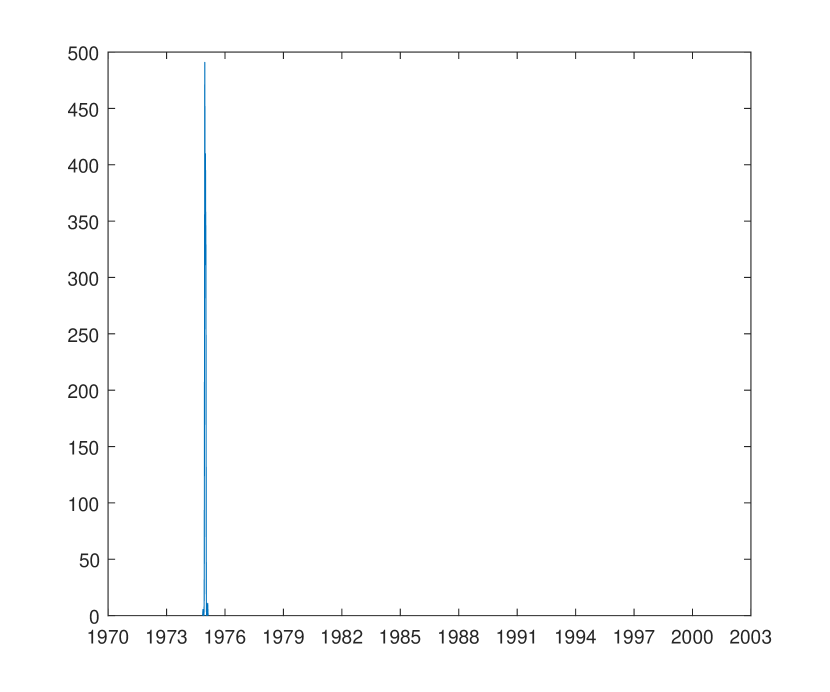
(a) United Kingdom

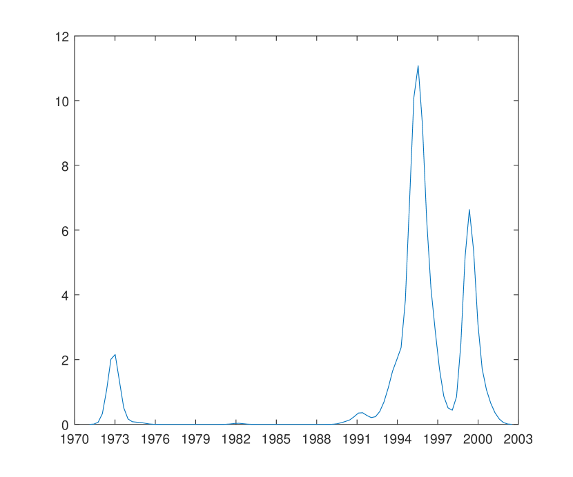
(b) Japan

Figure 3: Posterior density of the break date

slopes	Least-squares			Bayesian
	Estimate	LB	UB	Estimate	LB	UB
$\delta_{1}^{(1)}$	2.41	0.24	4.57	1.49	-1.89	5.27
$\delta_{1}^{(2)}$	1.17	0.44	1.89	1.31	0.29	3.26
$\delta_{1}^{(3)}$	-1.98	-2.45	-1.50	-2.00	-3.53	-1.23
$\delta_{1}^{(4)}$	-0.85	-1.55	-0.16	-0.29	-1.43	3.59
$\delta_{1}^{(5)}$	2.76	1.39	4.12	2.29	0.15	4.11
$\delta_{2}^{(1)}$	-16.8	-29.6	-4.07	-9.39	-23.4	8.77
$\delta_{2}^{(2)}$	12.4	2.35	22.4	6.22	-5.91	16.8
$\delta_{2}^{(3)}$	-7.11	-14.1	-0.04	-3.86	-13.1	5.32
$\delta_{2}^{(4)}$	4.76	1.25	8.27	1.70	-5.86	6.59
$\delta_{2}^{(5)}$	-8.35	-14.9	-1.78	-4.65	-12.1	4.98
$\tau$	Least-squares			Bayesian
	Estimate	LB	UB	Estimate	LB	UB
	0.780	0.777	0.782	0.779	0.068	0.934
	(96:05)	(96:04)	(96:06)	(96:05)	(72:03)	(01:10)
	ILR
	Estimate	LB	UB
		0.080	0.890
		(72:08)	(00:02)

• The upper panel shows point estimates as well as 90% confidence (left) and equal-tailed credible (right) intervals for the regression slope parameters. The lower panel shows point estimates of $\tau$ with the corresponding months in parentheses as well as the bounds of 95% confidence intervals of Bai (1997) and highest posterior density (HPD) sets. It also displays the inverted likelihood ratio (ILR) confidence sets of Eo  Morley (2015). LB=lower bound and UB=upper bound of the intervals.

Table 6: Estimation results for the Japanese stock return

In contrast, when the uncertainty on $\tau$ is large, the conventional and the Bayesian results on inference about the slope parameters might disagree. Table 6 shows the results for Japan. Although both $\hat{\tau}_{LS}$ and the posterior mode of $\tau$ are at 1996:05, the HPD set and the ILR confidence set are much wider than the confidence interval of Bai (1997), indicating a large uncertainty of the break date. The posterior density on $\tau$ in Figure 3 also illustrates that the uncertainty of the break date is much larger for Japan than for the U.K. during the sample period. The large uncertainty of $\tau$ is reflected on Bayesian inference on the slope parameters. In the upper panel of Table 6, we see that in general the Bayesian credible intervals are wider than the confidence intervals. Importantly, this can have a qualitative consequence on statistical importance of some parameters. For seven of the ten slope coefficients, the confidence intervals do not include zero while the the Bayesian credible intervals do. Hence, the conventional approach to inference on the slope parameters might not be robust with respect to the uncertainty of the break date, for the Japanese sample.

7 Conclusion and future direction

In this paper, we establish a Bernstein-von Mises type theorem for the slope coefficients in linear regression with a structural break. By doing so, we bridge the gap between the frequentist and the Bayesian approaches for inference on this model. On the one hand, a frequentist researcher can look at Bayesian credible intervals for the slope coefficients as a robustness check to see whether the uncertainty of the break location affects inference on the slope parameters. Such sensitivity analysis is natural as our theoretical result guarantees the credible interval to converge to the conventional confidence interval that the frequentist researcher would use otherwise. On the other hand, Bayesian inference can be conveyed to frequentists via our proven result.

Potential extensions include several directions. First, the homoscedasticity assumption could be too strong in some applications, and hence extending the results to the case of heteroscedasticity and autocorrelation would be of interest. Second, a popular Bayesian method of Chib (1998) is different from the approach we took in this paper in that we place an explicit prior on $\tau$ and that Chib’s framework can be naturally extended to the case of multiple breaks. It would be interesting to study frequentist properties of Chib’s approach.

Appendix A Proof of Theorems and Corollaries

In Appendix A, we provide proofs of Theorems 1-4 and Corollaries 1-2. See Appendix B for proofs of the Propositions used for proving the main theorems.

A.1 Proof of Theorem 1

Proof of Theorem 1.

Note that

$$\pi_{T}(\tau) =\frac{L_{T}(\tau)}{\int L_{T}(\tau^{\prime})d\tau^{\prime}}=\frac{L_{T}(\tau_{0})}{\int L_{T}(\tau^{\prime})d\tau^{\prime}}\frac{L_{T}(\tau)}{L_{T}(\tau_{0})}=\pi_{T}(\tau_{0})\frac{L_{T}(\tau)}{L_{T}(\tau_{0})},$$

$$\pi_{T}(\tau_{0}) =\frac{L_{T}(\tau_{0})}{\int L_{T}(\tau^{\prime})d\tau^{\prime}}\leq\frac{L_{T}(\tau_{0})}{\int_{B^{c}_{M_{0}/T}(\tau_{0})}L_{T}(\tau^{\prime})d\tau^{\prime}}=\bigg{[}\int_{B^{c}_{M_{0}/T}(\tau_{0})}\frac{L_{T}(\tau^{\prime})}{L_{T}(\tau_{0})}d\tau^{\prime}\bigg{]}^{-1},$$

for any $M_{0}>0$. Hence for each $T$ and for any $M_{0}>0$,

$$\int_{B^{c}_{M/T}(\tau_{0})}\pi_{T}(\tau)d\tau=\pi_{T}(\tau_{0})\int_{B^{c}_{M/T}(\tau_{0})}\frac{L_{T}(\tau)}{L_{T}(\tau_{0})}d\tau\leq\bigg{[}\int_{B^{c}_{M_{0}/T}(\tau_{0})}\frac{L_{T}(\tau^{\prime})}{L_{T}(\tau_{0})}d\tau^{\prime}\bigg{]}^{-1}\int_{B^{c}_{M/T}(\tau_{0})}\frac{L_{T}(\tau)}{L_{T}(\tau_{0})}d\tau.$$ (12)

Therefore, we want to find

1. an upper bound for $\int_{B^{c}_{M/T}(\tau_{0})}\frac{L_{T}(\tau)}{L_{T}(\tau_{0})}d\tau$ and

2. a lower bound for $\int_{B^{c}_{M_{0}/T}(\tau_{0})}\frac{L_{T}(\tau^{\prime})}{L_{T}(\tau_{0})}d\tau^{\prime}$ for some $M_{0}>0$

We can write the marginal likelihood ratio as

$$\frac{L_{T}(\tau)}{L_{T}(\tau_{0})}=\exp\bigg{[}T\left\{\frac{1}{T}\log\left(\frac{L_{T}(\tau)}{L_{T}(\tau_{0})}\right)\right\}\bigg{]}.$$

The proof of Theorem 1 is built on some intermediate steps, Propositions 1-4. Proposition 1 shows that, under the normal likelihood and the conjugate prior, studying this ratio boils down to comparing the sum of squared residuals $S_{T}(\tau)$.

Proposition 1.

Suppose Assumption 1 holds. Then, with the normal likelihood and the conjugate prior described above, under $P_{\theta_{0},\tau_{0}}$, for all $\tau$,

$$\frac{1}{T}\log\left(\frac{L_{T}(\tau)}{L_{T}(\tau_{0})}\right)=\frac{1}{2}\log\left(\frac{S_{T}(\tau_{0})}{S_{T}(\tau)}\right)+O_{p}(T^{-1}).$$

Let us first examine the limit of the quantity $Q_{T}(\tau)=T^{-1}S_{T}(\tau)$. Proposition 2 states that $Q_{T}(\tau)$ converges in probability to some deterministic function $Q(\tau)$. See Figure 2 for examples of $Q_{T}(\tau)$ and $Q(\tau)$.

Proposition 2.

Suppose Assumption 1 holds. Then, under $P_{\theta_{0},\tau_{0}}$, for all $\tau$,

$$Q_{T}(\tau)=Q(\tau)+O_{p}(T^{-1/2}),$$

where

$$Q(\tau)=\sigma_{0}^{2}+\begin{cases}(\tau_{0}-\tau)\frac{(1-\tau_{0})}{(1-\tau)}\delta_{0}^{\prime}R^{\prime}\Sigma_{X}R\delta_{0},&\text{if }\tau\leq\tau_{0}\\ (\tau-\tau_{0})\frac{\tau_{0}}{\tau}\text{ }\delta_{0}^{\prime}R^{\prime}\Sigma_{X}R\delta_{0},&\text{if }\tau>\tau_{0}\end{cases}\equiv\sigma_{0}^{2}+\Delta(\tau).$$

Define $A_{T}(\tau)=g\left(Q_{T}(\tau)\right)$ and $A(\tau)=g(Q(\tau))$ where $g(x)=-\frac{1}{2}\log(x)$. Due to Proposition 1, we can write

$$T^{-1}\log\left(\frac{L_{T}(\tau)}{L_{T}(\tau_{0})}\right)=A_{T}(\tau)-A_{T}(\tau_{0})+O_{p}(T^{-1}).$$ (13)

Proposition 3 below says that the limit $A(\tau)$ of $A_{T}(\tau)$ attains its maximum at $\tau_{0}$.

Proposition 3.

$A(\tau)$ attains its unique maximum at $\tau_{0}$

Proposition 4 establishes the modulus of continuity of the empirical process $\left\{A_{T}(\tau)-A_{T}(\tau_{0})\right\}-\left\{A(\tau)-A(\tau_{0})\right\}$ outside of a ball around $\tau_{0}$ with radius proportional to $T^{-1}$.

Proposition 4.

Suppose Assumption 1 holds. Then, under $\forall\eta>0$, $\forall\epsilon>0$, $\exists M>0$ and $k>0$ such that $T\geq k$ $\implies$

$$P_{\theta_{0},\tau_{0}}\left(\inf_{\tau\in B^{c}_{M/T}(\tau_{0})}\frac{|\left\{A_{T}(\tau)-A_{T}(\tau_{0})\right\}-\left\{A(\tau)-A(\tau_{0})\right\}|}{|\tau-\tau_{0}|}<\eta\right)>1-\epsilon.$$

By Proposition 3, $A(\cdot)$ attains its unique max at $\tau_{0}$. Note that the convex function $A(\tau)$ is not differentiable at $\tau_{0}$. Hence we have,

$$A(\tau)-A(\tau_{0}) <|\tau-\tau_{0}|B_{1},$$

$$A(\tau)-A(\tau_{0}) >|\tau-\tau_{0}|B_{2},$$

for some $B_{1},B_{2}<0$. By Proposition 4, given $\eta_{1}>0$, $\exists M>0:$ with $P_{\theta_{0},\tau_{0}}\to 1$,

$$A_{T}(\tau)-A_{T}(\tau_{0})<\eta_{1}|\tau-\tau_{0}|+A(\tau)-A(\tau_{0})<|\tau-\tau_{0}|\{\eta_{1}+B_{1}\},$$ (14)

for all $\tau\in B^{c}_{M/T}(\tau_{0})$. Similarly, given $\eta_{2}>0$, $\exists M_{0}>0:$ with $P_{\theta_{0},\tau_{0}}\to 1$,

$$A_{T}(\tau)-A_{T}(\tau_{0})>-\eta_{2}|\tau-\tau_{0}|+A(\tau)-A(\tau_{0})>|\tau-\tau_{0}|\{-\eta_{2}+B_{2}\},$$ (15)

for all $\tau\in B^{c}_{M_{0}/T}(\tau_{0})$. Recall, by Eq.(13), we have

$$\frac{L_{T}(\tau)}{L_{T}(\tau_{0})}=\exp\bigg{[}T\bigg{(}A_{T}(\tau_{0})-A_{T}(\tau)\bigg{)}+O_{p}(1)\bigg{]}.$$

Hence, from Eq. (14), given $\eta_{1}>0$, small compared to $-B_{1}$, there is $B_{1}^{\prime}<0$, which is independent of $M$: we have with $P_{\theta_{0},\tau_{0}}\to 1$,

$$\frac{L_{T}(\tau)}{L_{T}(\tau_{0})}\leq\exp\bigg{[}T|\tau-\tau_{0}|B^{\prime}_{1}+O_{p}(1)\bigg{]}=\exp\bigg{[}T|\tau-\tau_{0}|B^{\prime}_{1}\bigg{]}O_{p}(1),$$ (16)

for all $\tau\in B^{c}_{M/T}(\tau_{0})$. Note that the statement above still holds with a larger value of $M>0$ as the area outside of the ball will be contained by that for the original $M$. Similarly, from Eq. (15), there is $B_{2}^{\prime}<0$ and $M_{0}>0:$ with $P_{\theta_{0},\tau_{0}}\to 1$,

$$\frac{L_{T}(\tau)}{L_{T}(\tau_{0})}\geq\exp\bigg{[}T|\tau-\tau_{0}|B^{\prime}_{2}+O_{p}(1)\bigg{]}=\exp\bigg{[}T|\tau-\tau_{0}|B^{\prime}_{2}\bigg{]}O_{p}(1),$$ (17)

for all $\tau\in B^{c}_{M_{0}/T}(\tau_{0})$. Now, by Inequality (16) and the fundamental theorem of calculus,

$$\int_{B^{c}_{M/T}(\tau_{0})}\frac{L_{T}(\tau)}{L_{T}(\tau_{0})}d\tau\leq\int_{B^{c}_{M/T}(\tau_{0})}\exp\bigg{[}T|\tau-\tau_{0}|B^{\prime}_{1}\bigg{]}d\tau O_{p}(1)=\frac{1}{TB^{\prime}_{1}}\left(e^{TB^{\prime}_{1}}-e^{B^{\prime}_{1}M}\right)O_{p}(1).$$

Similarly, by Inequality (17),

$$\int_{B_{M_{0}^{c}/T}(\tau_{0})}\frac{L_{T}(\tau)}{L_{T}(\tau_{0})}d\tau\geq\int_{B_{M_{0}^{c}/T}(\tau_{0})}\exp\bigg{[}T|\tau-\tau_{0}|B^{\prime}_{2}\bigg{]}d\tau O_{p}(1)=\frac{1}{TB^{\prime}_{2}}\left(e^{TB^{\prime}_{2}}-e^{B^{\prime}_{2}M_{0}}\right)O_{p}(1).$$

This means, together with the bound (12),

$$\int_{B^{c}_{M/T}(\tau_{0})}\pi_{T}(\tau)d\tau\leq\bigg{[}\int_{B_{M^{c}_{0}/T}(\tau_{0})}\frac{L_{T}(\tau^{\prime})}{L_{T}(\tau_{0})}d\tau^{\prime}\bigg{]}^{-1}\int_{B^{c}_{M/T}(\tau_{0})}\frac{L_{T}(\tau)}{L_{T}(\tau_{0})}d\tau\leq\frac{B^{\prime}_{2}}{B^{\prime}_{1}}\frac{e^{B^{\prime}_{1}T}-e^{B^{\prime}_{1}M}}{e^{B^{\prime}_{2}T}-e^{B_{2}^{\prime}M_{0}}}O_{p}(1),$$

which can be made arbitrarily small by choosing $M>0$ and $T$ sufficiently large. ∎

A.2 Proof of Corollary 1

Proof of Corollary 1 .

The main structure of the proof follows Proposition 2 of Bai (1997) and relies on an implication of our Theorem 1. First, note that we have

$$\hat{\tau}_{Bayes} =\operatorname*{arg\,max}_{\tau\in\mathcal{H}}\pi_{T}(\tau)$$

$$=\operatorname*{arg\,max}_{\tau\in\mathcal{H}}L_{T}(\tau)$$

$$=\operatorname*{arg\,max}_{\tau\in\mathcal{H}}\frac{1}{T}\log\left(\frac{L_{T}(\tau)}{L_{T}(\tau_{0})}\right),$$

which converges in distribution to $\operatorname*{arg\,max}_{\tau\in\mathcal{H}}\log\left(\frac{S_{T}(\tau_{0})}{S_{T}(\tau)}\right)$ by Proposition 1. We have

$$\operatorname*{arg\,max}_{\tau\in\mathcal{H}}\log\left(\frac{S_{T}(\tau_{0})}{S_{T}(\tau)}\right) =\operatorname*{arg\,min}_{\tau\in\mathcal{H}}S_{T}(\tau)$$

$$=\operatorname*{arg\,max}_{\tau\in\mathcal{H}}V_{T}(\tau)-V_{T}(\tau_{0}),$$

where $V_{T}(\tau)=\hat{\delta}(\tau)^{\prime}\left(Z_{2}^{\prime}MZ_{2}\right)\hat{\delta}(\tau)$. Bai (1997) shows that $V_{T}(\tau)-V_{T}(\tau_{0})$ converges in distribution to $W^{*}\left(\left\lfloor T(\tau-\tau_{0})\right\rfloor\right)$ uniformly on any bounded interval around $\tau_{0}$. Let $m^{*}=\operatorname*{arg\,max}_{m}W^{*}(m)$, which is $O_{p}(1)$. Hence, $\forall\epsilon>0$, $\exists R_{1}>0:$ $P\left(|m^{*}|>R_{1}\right)<\epsilon$. Our Theorem 1 implies that $\hat{\tau}_{Bayes}=\tau_{0}+O_{p}(T^{-1})$. In other words, $\forall\epsilon>0$, $\exists R_{2}>0:$ $P\left(T|\hat{\tau}_{Bayes}-\tau_{0}|>R_{2}\right)<\epsilon$. Take $R=\max\{R_{1},R_{2}\}$.

Define $\hat{\tau}_{R}=\operatorname*{arg\,max}_{T|\tau-\tau_{0}|\leq R}V_{T}(\tau)-V_{T}(\tau_{0})$ and $m^{*}_{R}=\operatorname*{arg\,max}_{|m|\leq R}W^{*}(m)$. Then we have $T|\hat{\tau}_{R}-\tau_{0}|\overset{d}{\to}m^{*}_{R}$. In other words, $\big{|}P\left(\left\lfloor T(\hat{\tau}_{R}-\tau_{0})\right\rfloor=j\right)-P\left(m^{*}_{R}=j\right)\big{|}<\epsilon$ as $T\to\infty$ $\forall|j|\leq R$.

Note that if $T|\hat{\tau}_{Bayes}-\tau_{0}|<R$, then $\hat{\tau}_{R}=\hat{\tau}_{Bayes}$. Similarly, if $|m^{*}|<R$, then $m^{*}_{R}=m^{*}$. Hence, $\big{|}P\left(\left\lfloor T(\hat{\tau}_{Bayes}-\tau_{0})\right\rfloor=j\right)-P\left(m^{*}=j\right)\big{|}$ is bounded by $\big{|}P\left(\left\lfloor T(\hat{\tau}_{R}-\tau_{0})\right\rfloor=j\right)-P\left(m^{*}_{R}=j\right)\big{|}+P\left(T|\hat{\tau}_{Bayes}-\tau_{0}|\geq R\right)+P\left(|m^{*}|\geq R\right)<3\epsilon$. As $\epsilon$ can be made arbitrarily small, the desired result holds.

∎

A.3 Proof of Theorem 2

Proof of Theorem 2 .

Define $z=\sqrt{T}\left(\gamma-\hat{\gamma}_{LS}\right)$ and let $\phi(x;\mu,\Sigma)$ be the multivariate normal density with mean $\mu$ and covariance matrix $\Sigma$ evaluated at $x$.

$$d_{TV}\bigg{(}\pi\left[z|\bm{D}_{T}\right],N_{(d_{x}+d_{z})}\left(0,\sigma_{0}^{2}V^{-1}\right)\bigg{)}=\int|\pi(z|\bm{D}_{T})-\phi(z;0,\sigma_{0}^{2}V^{-1})|dz$$

$$\leq\int\int|\pi(z|\tau,\bm{D}_{T})-\phi(z;0,\sigma_{0}^{2}V^{-1})|dzd\pi(\tau|\bm{D}_{T})$$

$$=\int d_{TV}\bigg{(}\pi(z|\tau,\bm{D}_{T}),\phi(z;0,\sigma_{0}^{2}V^{-1})\bigg{)}d\pi(\tau|\bm{D}_{T})$$

$$=\int_{B_{M/T}(\tau_{0})}d_{TV}\bigg{(}\pi(z|\tau,\bm{D}_{T}),\phi(z;0,\sigma_{0}^{2}V^{-1})\bigg{)}d\pi(\tau|\bm{D}_{T})+o_{p}(1),$$

where the last equality is due to Theorem 1.

From (10), asymptotically, the posterior of $\gamma$ conditional on $\tau$ is normal:

$$\gamma\big{|}\tau,\bm{D}_{T} \overset{a}{\sim}N_{(d_{x}+d_{z})}\left(\bar{\mu}_{\tau},(\bar{b}_{\tau}/\bar{a})\bar{H}_{\tau}^{-1}\right)$$

$$\implies z|\tau,\bm{D}_{T} \overset{a}{\sim}N_{(d_{x}+d_{z})}\left(\sqrt{T}\left(\bar{\mu}_{\tau}-\hat{\gamma}_{LS}\right),(T\bar{b}_{\tau}/\bar{a})\bar{H}_{\tau}^{-1}\right).$$

The total variation distance is bounded above by 2 times square root of the KL divergence. In general, the KL divergence between two $p$-dimensional normal distributions $N_{p}(\mu_{1},\Sigma_{1})$ and $N_{p}(\mu_{2},\Sigma_{2})$ is bounded above by

$$\underbrace{\frac{\left|\det\left(\Sigma_{2}^{-1}\right)-\det\left(\Sigma_{1}^{-1}\right)\right|}{\min(\det\left(\Sigma_{1}^{-1}\right),\det\left(\Sigma_{2}^{-1}\right))}}_{I}+\underbrace{p||\Sigma_{2}^{-1}-\Sigma_{1}^{-1}||_{\infty}||\Sigma_{1}||_{\infty}}_{II}+\underbrace{||\mu_{1}-\mu_{2}||_{2}^{2}||\Sigma_{2}^{-1}||_{2}}_{III},$$ (18)

where $||\Sigma||_{\infty}=max_{ij}|\Sigma_{ij}|$ is the largest element of $\Sigma$ in the absolute value, and $||\Sigma||_{2}=sup_{\mu}||\Sigma\mu||_{2}/||\mu||_{2}$ is a matrix norm induced by the standard norm on $\mathbb{R}^{p}$, $||\mu||_{2}=\sum_{i=1}^{p}\mu_{i}^{2}$. We can bound the total variation distance between the posterior density of $z$ conditional on $\tau$ and that of $N_{(d_{x}+d_{z})}(0,\sigma_{0}^{2}V^{-1})$ using the bound (18), with $\mu_{1}=\sqrt{T}\left(\bar{\mu}_{\tau}-\hat{\gamma}_{LS}\right)$, $\Sigma_{1}=(T\bar{b}_{\tau}/\bar{a})\bar{H}_{\tau}^{-1}$, $\mu_{2}=0$, and $\Sigma_{2}=\sigma_{0}^{2}V^{-1}$.

To show $III=o_{p}(1)$, we write

$$\sqrt{T}\left(\bar{\mu}_{\tau}-\hat{\gamma}_{LS}\right)=\sqrt{T}\left(\bar{\mu}_{\tau}-\hat{\gamma}(\tau)\right)+\sqrt{T}\left(\hat{\gamma}(\tau)-\hat{\gamma}_{LS}\right).$$ (19)

By definition,

$$\bar{\mu}_{\tau}=\left[\frac{1}{T}\underline{H}+\frac{1}{T}\chi_{\tau}^{\prime}\chi_{\tau}\right]^{-1}\left[\frac{1}{T}\underline{H}\underline{\mu}+\frac{1}{T}\chi_{\tau}Y\right]=\hat{\gamma}(\tau)+O_{p}(T^{-1}),$$

so the first term in (19) is $o_{p}(1)$. To show that the second term in (19) is $o_{p}(1)$ for $\tau\in B_{M/T}(\tau_{0})$, write $\sqrt{T}\left(\hat{\gamma}(\tau)-\hat{\gamma}_{LS}\right)=\sqrt{T}\left(\hat{\gamma}(\tau)-\gamma_{0}\right)-\sqrt{T}\left(\hat{\gamma}_{LS}-\gamma_{0}\right)$. Note that $Y=X\beta_{0}+Z_{2\tau_{0}}\delta_{0}+\epsilon=X\beta_{0}+Z_{2\tau}\delta_{0}+\epsilon_{\tau}^{*}$, where $\epsilon_{\tau}^{*}=(Z_{2\tau_{0}}-Z_{2\tau})\delta_{0}+\epsilon$. This implies

$$\sqrt{T}\left(\hat{\gamma}(\tau)-\gamma_{0}\right) =\left[\frac{1}{T}\begin{pmatrix}X^{\prime}X&X^{\prime}Z_{2\tau}\\ Z_{2\tau}^{\prime}X&Z_{2\tau}^{\prime}Z_{2\tau}\end{pmatrix}\right]^{-1}\frac{1}{\sqrt{T}}\begin{pmatrix}X^{\prime}\epsilon_{\tau}^{*}\\ Z_{2\tau}^{\prime}\epsilon_{\tau}^{*}\end{pmatrix}$$

$$=\left[\frac{1}{T}\begin{pmatrix}X^{\prime}X&X^{\prime}Z_{2\tau}\\ Z_{2\tau}^{\prime}X&Z_{2\tau}^{\prime}Z_{2\tau}\end{pmatrix}\right]^{-1}\frac{1}{\sqrt{T}}\begin{pmatrix}X^{\prime}\epsilon+X^{\prime}(Z_{2\tau_{0}}-Z_{2\tau})\delta_{0}\\ Z_{2\tau}^{\prime}\epsilon+Z_{2\tau_{0}}^{\prime}(Z_{2\tau_{0}}-Z_{2\tau})\delta_{0}\end{pmatrix}.$$

For $|\tau-\tau_{0}|<\frac{M}{T}$, we have

$$\frac{1}{T}X^{\prime}Z_{2\tau}-\frac{1}{T}X^{\prime}Z_{2\tau_{0}} =o_{p}(1),\quad\frac{1}{T}Z_{2\tau}^{\prime}Z_{2\tau}-\frac{1}{T}Z_{2\tau_{0}}^{\prime}Z_{2\tau_{0}}=o_{p}(1),$$

$$\quad\frac{1}{\sqrt{T}}X^{\prime}(Z_{2\tau_{0}}-Z_{2\tau}) =o_{p}(1),\quad\frac{1}{\sqrt{T}}Z_{2\tau_{0}}^{\prime}(Z_{2\tau_{0}}-Z_{2\tau})=o_{p}(1),$$

$$\quad\frac{1}{\sqrt{T}}Z_{2\tau}^{\prime}\epsilon-\frac{1}{\sqrt{T}}Z_{2\tau_{0}}\epsilon =o_{p}(1),$$

which implies

$$\sqrt{T}\left(\hat{\gamma}(\tau)-\gamma_{0}\right)=\left[\frac{1}{T}\begin{pmatrix}X^{\prime}X&X^{\prime}Z_{2\tau_{0}}\\ Z_{2\tau_{0}}^{\prime}X&Z_{2\tau_{0}}^{\prime}Z_{2\tau_{0}}\end{pmatrix}\right]^{-1}\frac{1}{\sqrt{T}}\begin{pmatrix}X^{\prime}\epsilon\\ Z_{2\tau_{0}}^{\prime}\epsilon\end{pmatrix}+o_{p}(1).$$

Similarly, since the least-square estimator $\hat{\tau}_{LS}\in B_{M/T}(\tau_{0})$ for sufficiently large $T$, we can show

$$\sqrt{T}\left(\hat{\gamma}_{LS}-\gamma_{0}\right) =\sqrt{T}\left(\hat{\gamma}(\hat{\tau}_{LS})-\gamma_{0}\right)$$

$$=\left[\frac{1}{T}\begin{pmatrix}X^{\prime}X&X^{\prime}Z_{2\hat{\tau}_{LS}}\\ Z_{2\hat{\tau}_{LS}}^{\prime}X&Z_{2\hat{\tau}_{LS}}^{\prime}Z_{2\hat{\tau}_{LS}}\end{pmatrix}\right]^{-1}\frac{1}{\sqrt{T}}\begin{pmatrix}X^{\prime}\epsilon+X^{\prime}(Z_{2\tau_{0}}-Z_{2\hat{\tau}_{LS}})\delta_{0}\\ Z_{2\hat{\tau}_{LS}}^{\prime}\epsilon+Z_{2\tau_{0}}^{\prime}(Z_{2\tau_{0}}-Z_{2\hat{\tau}_{LS}})\delta_{0}\end{pmatrix}$$

$$=\left[\frac{1}{T}\begin{pmatrix}X^{\prime}X&X^{\prime}Z_{2\tau_{0}}\\ Z_{2\tau_{0}}^{\prime}X&Z_{2\tau_{0}}^{\prime}Z_{2\tau_{0}}\end{pmatrix}\right]^{-1}\frac{1}{\sqrt{T}}\begin{pmatrix}X^{\prime}\epsilon\\ Z_{2\tau_{0}}^{\prime}\epsilon\end{pmatrix}+o_{p}(1).$$

Hence, $\sqrt{T}\left(\hat{\gamma}(\tau)-\hat{\gamma}_{LS}\right)=o_{p}(1)$.

To show $I$ and $II$ are $o_{p}(1)$, note that $\Sigma_{1}-\Sigma_{2}$ equals to

$$(T\bar{b}_{\tau}/\bar{a})\bar{H}_{\tau}^{-1}-\sigma^{2}_{0}V^{-1} =\left[(T\bar{b}_{\tau}/\bar{a})\bar{H}_{\tau}^{-1}-\frac{TS_{T}(\tau)}{T-(d_{x}+d_{z})}(\chi_{\tau}\chi_{\tau})^{-1}\right]+\left[\frac{TS_{T}(\tau)}{T-(d_{x}+d_{z})}(\chi_{\tau}\chi_{\tau})^{-1}-\sigma^{2}_{0}V^{-1}\right].$$ (20)

For the first term in (20), we have

$$(T\bar{b}_{\tau}/\bar{a})\bar{H}_{\tau}^{-1} =\frac{\bar{b}_{\tau}}{\underline{a}+T/2}\left[\frac{1}{T}\underline{H}+\frac{1}{T}\chi_{\tau}^{\prime}\chi_{\tau}\right]^{-1}=\frac{\frac{1}{T}\bar{b}_{\tau}}{\underline{a}/T+1/2}\left[\frac{1}{T}\underline{H}+\frac{1}{T}\chi_{\tau}^{\prime}\chi_{\tau}\right]^{-1}.$$

Note that $(1/T)\bar{b}_{\tau}=\frac{1}{2T}S_{T}(\tau)+O_{p}(T^{-1})$, so we have $(T\bar{b}_{\tau}/\bar{a})\bar{H}_{\tau}^{-1}=S_{T}(\tau)\left[\chi_{\tau}^{\prime}\chi_{\tau}\right]^{-1}+O_{p}(T^{-1}).$ Therefore, the term in the first square brackets in (20) is $o_{p}(1)$. For the second term in (20), we have that for $|\tau-\tau_{0}|<\frac{M}{T}$,

$$\frac{TS_{T}(\tau)}{T-(d_{x}+d_{z})}(\chi_{\tau}\chi_{\tau})^{-1}-\sigma^{2}_{0}V^{-1} =\underbrace{\left(Q_{T}(\tau)-Q_{T}(\tau_{0})\right)}_{=o_{p}(1)}\hat{V}^{-1}_{T}(\tau)+Q_{T}(\tau_{0})\underbrace{\left(\hat{V}^{-1}_{T}(\tau)-\hat{V}^{-1}_{T}(\tau_{0})\right)}_{=o_{p}(1)}$$

$$+\underbrace{\left(Q_{T}(\tau_{0})-\sigma_{0}^{2}\right)}_{=O_{p}(T^{-1/2})}\hat{V}^{-1}_{T}(\tau_{0})+\sigma_{0}^{2}\underbrace{\left(\hat{V}^{-1}_{T}(\tau_{0})-V^{-1}\right)}_{=o_{p}(1)}+o_{p}(1)=o_{p}(1),$$

where $\hat{V}_{T}(\tau)=\frac{1}{T}\chi_{\tau}^{\prime}\chi_{\tau}$.

This implies that $\Sigma_{2}^{-1}-\Sigma_{1}^{-1}=o_{p}(1)$. Hence $II=o_{p}(1)$. By continuity of determinants, we also have that $I=o_{p}(1)$ for $\tau\in B_{M/T}(\tau_{0})$.

Finally, for $\tau\in B_{M/T}(\tau_{0})$

$$d_{TV}\left(\pi(z|\tau,\bm{D}_{T}),N_{(d_{x}+d_{z})}(0,\sigma_{0}^{2}V)\right)\leq 2\sqrt{o_{p}(1)}=o_{p}(1).$$

This implies that $d_{TV}\bigg{(}\pi\left[z|\bm{D}_{T}\right],N_{(d_{x}+d_{z})}(0,\sigma_{0}^{2}V^{-1})\bigg{)}$ is bounded above by

$$\int_{B_{M/T}(\tau_{0})}d_{TV}\bigg{(}\pi(z|\tau,\bm{D}_{T}),\phi(z;0,\sigma_{0}^{2}V^{-1})\bigg{)}d\pi(\tau|\bm{D}_{T})+o_{p}(1)=o_{p}(1).$$

∎

A.4 Proof of Theorem 3

Proof of Theorem 3 .

Recall that the proof of Theorem 1 is an implication of Propositions 1-4. Assumption 1 implies Propositions 2-4. Proposition 1 establishes that under the normal likelihood and the conjugate prior, Assumption 1 implies

$$\frac{1}{T}\log\left(\frac{L_{T}(\tau)}{L_{T}(\tau_{0})}\right) =\frac{1}{2}\log\left(\frac{S_{T}(\tau_{0})}{S_{T}(\tau)}\right)+O_{p}(T^{-1}).$$ (21)

Therefore, Theorem 3 can be proved if we establish the above equality under the normal likelihood and the prior described in Section 4, together with Assumptions 1-2.

For a given $\tau$, denote by $F_{T}(\theta,\tau)=\log p(\bm{Y}_{T}|\bm{X}_{T},\theta,\tau)$ the log likelihood function conditional on $\tau$. Under the normal likelihood and Assumption 1, together with Assumption 2, we can involke Theorem 3 of Hong  Preston (2012) (see their page 361) which establishes that

$$\log\int e^{F_{T}(\theta,\tau)-F_{T}(\hat{\theta}(\tau),\tau)}\pi(\theta,\tau)d\theta=\log\left[\pi(\theta^{*}(\tau),\tau)(2\pi)^{(d_{x}+d_{z}+1)/2}\det\left(-TA_{\theta}(\tau)\right)^{-1/2}\right]+o_{p}(1),$$

for each $\tau$, where $-A_{\theta}(\tau)$ is the probability limit of $-\frac{1}{T}\frac{\partial^{2}}{\partial\theta\partial\theta^{\prime}}F_{T}\left(\hat{\theta}(\tau),\tau\right)$ and is positive definite.

Note that

$$\frac{L_{T}(\tau)}{L_{T}(\tau_{0})} =\frac{e^{F_{T}(\hat{\theta}(\tau),\tau)}\int e^{F_{T}(\theta,\tau)-F_{T}(\hat{\theta}(\tau),\tau)}\pi(\theta,\tau)d\theta}{e^{F_{T}(\hat{\theta}(\tau_{0}),\tau_{0})}\int e^{F_{T}(\theta,\tau_{0})-F_{T}(\hat{\theta}(\tau_{0}),\tau_{0}))}\pi(\theta,\tau_{0})d\theta},$$

which implies that

$$\frac{1}{T}\log\left(\frac{L_{T}(\tau)}{L_{T}(\tau_{0})}\right) =\frac{1}{T}F_{T}(\hat{\theta}(\tau),\tau)-\frac{1}{T}F_{T}(\hat{\theta}(\tau_{0}),\tau_{0})$$

$$+\frac{1}{T}\log\left[\pi(\theta^{*}(\tau),\tau)(2\pi)^{(d_{x}+d_{z}+1)/2}\det\left(-TA_{\theta}(\tau)\right)^{-1/2}\right]$$

$$-\frac{1}{T}\log\left[\pi(\theta^{*}(\tau_{0}),\tau_{0})(2\pi)^{(d_{x}+d_{z}+1)/2}\det\left(-TA_{\theta}(\tau_{0})\right)^{-1/2}\right]+O_{p}(T^{-1})$$

$$=\frac{1}{T}\log\left[\frac{p(\bm{Y}_{T}|\bm{X}_{T},\hat{\theta}(\tau),\tau)}{p(\bm{Y}_{T}|\bm{X}_{T},\hat{\theta}(\tau_{0}),\tau_{0})}\right]+\frac{1}{T}\log\left[\frac{\pi\left(\theta^{*}(\tau),\tau\right)}{\pi\left(\theta^{*}(\tau_{0}),\tau_{0}\right)}\right]$$

$$-\frac{1}{2T}\log\left[\frac{\det\left(-A_{\theta}(\tau)\right)}{\det\left(-A_{\theta}(\tau_{0})\right)}\right]+O_{p}(T^{-1}).$$

Note that we assumed that $\pi\left(\theta^{*}(\tau),\tau\right)$ and $\pi\left(\theta^{*}(\tau_{0}),\tau_{0}\right)$ are finite and non-zero. Hence, the term involving the ratio of the priors is $O_{p}(T^{-1})$. Also, $-A_{\theta}(\tau)$ is a positive definite matrix hence its determinant is a finite positive number. We have

$$p(\bm{Y}_{T}|\bm{X}_{T},\hat{\theta}(\tau),\tau)\propto\left(\frac{1}{\hat{\sigma}^{2}(\tau)}\right)^{T/2}\exp\bigg{[}-\frac{1}{2\hat{\sigma}^{2}(\tau)}\underbrace{\sum_{t=1}^{T}\left(y_{t}-\chi_{\tau,t}\hat{\gamma}(\tau)\right)^{2}}_{=S_{T}(\tau)}\bigg{]}=\left(\frac{1}{\hat{\sigma}^{2}(\tau)}\right)^{T/2}\exp\left(-T/2\right),$$

where the last equality is due to the fact that $\hat{\sigma}^{2}(\tau)=S_{T}(\tau)/T$. This implies the desired result i.e., (21). Note that Propositions 2-4 hold under Assumption 1. Therefore, given (21), the rest of the proof of Theorem 3 follows the same argument in the proof of Theorem 1 in A.1. ∎

A.5 Proof of Corollary 2

Proof of Corollary 2 .

Note that

$$\hat{\tau}_{Bayes} =\operatorname*{arg\,max}_{\tau\in\mathcal{H}}\pi_{T}(\tau)=\operatorname*{arg\,max}_{\tau\in\mathcal{H}}\frac{1}{T}\log\left(\frac{L_{T}(\tau)}{L_{T}(\tau_{0})}\right),$$

converges in distribution to $\operatorname*{arg\,max}_{\tau\in\mathcal{H}}\log\left(\frac{S_{T}(\tau_{0})}{S_{T}(\tau)}\right)$ due to (21), under the normal likelihood and the assumed condition on the prior, together with Assumptions 1-2. Furthermore, Theorem 3 implies that $\hat{\tau}_{Bayes}=\tau_{0}+O_{p}(T^{-1})$. Based on these two facts, the rest of the proof follows the same argument as in the proof of Corollary 1 in A.2.

∎

A.6 Proof of Theorem 4

Proof of Theorem 4 .

Under the normal likelihood and Assumptions 1-2, a result from Hong  Preston (2012) (see their page 367) implies that the posterior of $\sqrt{T}\left(\gamma-\hat{\gamma}(\tau)\right)$ conditional on $\tau$ converges in total variation in probability to the multivariate normal distribution $N(0,-A_{\gamma}^{-1}(\tau))$, where $A_{\gamma}^{-1}(\tau)$ is the sub-matrix of $A_{\theta}^{-1}(\tau)$ obtained by deleting the last row and the last column, $-A_{\theta}(\tau)$ is the probability limit of $-\frac{1}{T}\frac{\partial^{2}}{\partial\theta\partial\theta^{\prime}}F_{T}\left(\hat{\theta}(\tau),\tau\right)$, and $F_{T}(\theta,\tau)=\log p(\bm{Y}_{T}|\bm{X}_{T},\theta,\tau)$ is the log likelihood function conditional on $\tau$. This means that the total variation between the posterior of $z=\sqrt{T}\left(\gamma-\hat{\gamma}_{LS}\right)$ given $\tau$ and $N\left(\sqrt{T}\left(\hat{\gamma}(\tau)-\hat{\gamma}_{LS}\right),-A_{\gamma}^{-1}(\tau)\right)$ converges to 0 in probability.

The bound (18) on the KL divergence between two normal densities can be used again now with $\mu_{2}=0$, $\Sigma_{2}=\sigma_{0}^{2}V^{-1}$, $\mu_{1}=\sqrt{T}\left(\hat{\gamma}(\tau)-\hat{\gamma}_{LS}\right)$, and $\Sigma_{1}=-A_{\gamma}^{-1}(\tau)=\text{plim }\hat{\sigma}^{2}(\tau)\hat{V}_{T}^{-1}(\tau)$ where $\hat{V}_{T}(\tau)=\frac{1}{T}\chi_{\tau}^{\prime}\chi_{\tau}$. Note that from the proof of Theorem 2 in A.3, we know that $\mu_{1}=o_{p}(1)$ for $|\tau-\tau_{0}|<\frac{M}{T}$.

For $|\tau-\tau_{0}|<\frac{M}{T}$,

$$\Sigma_{1}-\Sigma_{2} =\underbrace{-A_{\gamma}^{-1}(\tau)-Q_{T}(\tau)\hat{V}_{T}^{-1}(\tau)}_{=o_{p}(1)}$$

$$+\underbrace{\left(Q_{T}(\tau)-Q_{T}(\tau_{0})\right)}_{=o_{p}(1)}\hat{V}^{-1}_{T}(\tau)$$

$$+Q_{T}(\tau_{0})\underbrace{\left(\hat{V}^{-1}_{T}(\tau)-\hat{V}^{-1}_{T}(\tau_{0})\right)}_{=o_{p}(1)}$$

$$+\underbrace{\left(Q_{T}(\tau_{0})-\sigma_{0}^{2}\right)}_{=O_{p}(T^{-1/2})}\hat{V}^{-1}_{T}(\tau_{0})$$

$$+\sigma_{0}^{2}\underbrace{\left(\hat{V}^{-1}_{T}(\tau_{0})-V^{-1}\right)}_{=o_{p}(1)}+o_{p}(1)=o_{p}(1),$$

which implies

$$\Sigma_{2}^{-1}-\Sigma_{1}^{-1}=o_{p}(1).$$

The rest of the proof can be done similarly as in the proof of Theorem 2 in A.3 by applying the bound (18). ∎

Appendix B Proof of Propositions

B.1 Proof of Proposition 1

See 1

Proof of Proposition 1.

From (9), we have

$$\frac{1}{T}\log\left(\frac{L_{T}(\tau)}{L_{T}(\tau_{0})}\right) =\frac{1}{2T}\log\left[\frac{\det\left(\bar{H}_{\tau_{0}}\right)}{\det\left(\bar{H}_{\tau}\right)}\right]+\frac{\bar{a}}{T}\log\bigg{[}\frac{\bar{b}_{\tau_{0}}}{\bar{b}_{\tau}}\bigg{]}+\frac{1}{T}\log\bigg{(}\frac{\pi(\tau)}{\pi(\tau_{0})}\bigg{)}.$$

Assumption 1 implies that each component of $(1/T)\chi_{\tau}^{\prime}\chi_{\tau}$ converges in probability to a constant matrix. By continuity of determinant, the determinant converges to the determinant of the limiting matrix. As a result, the quantity inside of log in the first term is $O_{p}(1)$ and hence the first term is $O_{p}(T^{-1})$. By the choice of the prior, the ratio $\pi(\tau)/\pi(\tau_{0})$ is bounded, so the last term is $O(T^{-1})$. Note that

$$(1/T)\bar{b}_{\tau} =(1/T)\underline{b}+\frac{1}{2T}\left[\underline{\mu}^{\prime}\underline{H}\underline{\mu}+Y^{\prime}Y-\bar{\mu}_{\tau}^{\prime}\bar{H}_{\tau}\bar{\mu}_{\tau}\right]$$

$$=\frac{1}{2T}\left[Y^{\prime}Y-(\chi_{\tau}^{\prime}Y)^{\prime}(\chi_{\tau}^{\prime}\chi_{\tau})^{-1}(\chi_{\tau}^{\prime}Y)\right]+O_{p}(T^{-1})$$

$$=\frac{1}{2T}S_{T}(\tau)+O_{p}(T^{-1}).$$ (22)

Hence, we conclude that

$$\frac{1}{T}\log\left(\frac{L_{T}(\tau)}{L_{T}(\tau_{0})}\right)=\frac{1}{2}\log\bigg{(}\frac{S_{T}(\tau_{0})}{S_{T}(\tau)}\bigg{)}+O_{p}(T^{-1}).$$

∎

B.2 Proof of Proposition 2

See 2

Proof of Proposition 2.

Let $\tau\in(0,1)$ be given. Let $M=I-X(X^{\prime}X)^{-1}X^{\prime}$. We have the following identity: $S_{T}(\tau)=\bar{S}_{T}-V_{T}(\tau)$ (Amemiya, 1985; Bai, 1997), where $\bar{S}_{T}$ is the sum of squared residuals from regressing $Y$ on $X$ alone and $V_{T}(\tau)=\hat{\delta}^{\prime}(\tau)(Z_{2\tau}^{\prime}MZ_{2\tau})\hat{\delta}(\tau)$. By Frisch-Waugh Theorem, the OLS estimate of $\delta$ in Eq. (4) is equivalent to that in the model $MY=MZ_{2\tau}\delta+M\epsilon$. Note the true model is $MY=MZ_{2\tau_{0}}\delta_{0}+M\epsilon$. Hence,

$$\hat{\delta}(\tau) =(Z_{2\tau}^{\prime}MZ_{2\tau})^{-1}Z_{2\tau}^{\prime}MY$$

$$=(Z_{2\tau}^{\prime}MZ_{2\tau})^{-1}Z_{2\tau}^{\prime}\left\{MZ_{2\tau_{0}}\delta_{0}+M\epsilon\right\}$$

$$=(Z_{2\tau}^{\prime}MZ_{2\tau})^{-1}Z_{2\tau}^{\prime}MZ_{2\tau_{0}}\delta_{0}+(Z_{2\tau}^{\prime}MZ_{2\tau})^{-1}Z_{2\tau}^{\prime}M\epsilon.$$

We have

$$V_{T}(\tau) =\delta_{0}^{\prime}(Z_{2\tau}^{\prime}MZ_{2\tau_{0}})^{\prime}(Z_{2\tau}^{\prime}MZ_{2\tau})^{-1}(Z_{2\tau}^{\prime}MZ_{2\tau_{0}})\delta_{0}$$

$$+2\delta_{0}^{\prime}(Z_{2\tau}^{\prime}MZ_{2\tau_{0}})^{\prime}(Z_{2\tau}^{\prime}MZ_{2\tau})^{-1}(Z_{2\tau}^{\prime}M\epsilon)$$

$$+(Z_{2\tau}^{\prime}M\epsilon)^{\prime}(Z_{2\tau}^{\prime}MZ_{2\tau})^{-1}(Z_{2\tau}^{\prime}M\epsilon).$$

By Assumption 1 (i),(ii), and (iv),

$$\frac{1}{T}V_{T}(\tau) =\frac{1}{T}\delta_{0}^{\prime}(Z_{2\tau}^{\prime}MZ_{2\tau_{0}})^{\prime}(Z_{2\tau}^{\prime}MZ_{2\tau})^{-1}(Z_{2\tau}^{\prime}MZ_{2\tau_{0}})\delta_{0}+O_{p}(T^{-1/2}).$$

Also we have

$$\bar{S}_{T} =Y^{\prime}MY=\delta_{0}^{\prime}Z_{2\tau_{0}}^{\prime}MZ_{2\tau_{0}}\delta_{0}+2\delta_{0}Z_{2\tau_{0}}M+\epsilon^{\prime}M\epsilon,$$

which implies

$$\frac{1}{T}\bar{S}_{T} =\frac{1}{T}\delta_{0}^{\prime}Z_{2\tau_{0}}^{\prime}MZ_{2\tau_{0}}\delta_{0}+\sigma_{0}^{2}+O_{p}(T^{-1/2}).$$

By the above identity, $Q_{T}(\tau)=\frac{1}{T}\bar{S}_{T}-\frac{1}{T}V_{T}(\tau)$ equals to

$$\sigma_{0}^{2}+\frac{1}{T}\delta_{0}^{\prime}\bigg{\{}(Z_{2\tau_{0}}^{\prime}MZ_{2\tau_{0}})-(Z_{2\tau}^{\prime}MZ_{2\tau_{0}})^{\prime}(Z_{2\tau}^{\prime}MZ_{2\tau})^{-1}(Z_{2\tau}^{\prime}MZ_{2\tau_{0}})\bigg{\}}\delta_{0}+O_{p}(T^{-1/2}).$$

Note that

$$(Z_{2\tau_{0}}^{\prime}MZ_{2\tau_{0}}) =Z_{2\tau_{0}}^{\prime}Z_{2\tau_{0}}-Z_{2\tau_{0}}^{\prime}X(XX^{\prime})^{-1}X^{\prime}Z_{2\tau_{0}}$$

$$=R^{\prime}X_{2\tau_{0}}^{\prime}X_{2\tau_{0}}R-R^{\prime}(X_{2\tau_{0}}^{\prime}X)(XX^{\prime})^{-1}(X^{\prime}X_{2\tau_{0}})R$$

$$=R^{\prime}X_{2\tau_{0}}^{\prime}X_{2\tau_{0}}R-R^{\prime}(X_{2\tau_{0}}^{\prime}X_{2\tau_{0}})(XX^{\prime})^{-1}(X_{2\tau_{0}}^{\prime}X_{2\tau_{0}})R.$$

By Assumption 1 (iii) and (iv),

$$\frac{1}{T}(Z_{2\tau_{0}}^{\prime}MZ_{2\tau_{0}}) =(1-\tau_{0})R^{\prime}\Sigma_{X}R-(1-\tau_{0})^{2}R^{\prime}\Sigma_{X}R+O_{p}(T^{-1/2})$$

$$=\tau_{0}(1-\tau_{0})R^{\prime}\Sigma_{X}R+O_{p}(T^{-1/2}).$$

Similarly,

$$\frac{1}{T}(Z_{2\tau}^{\prime}MZ_{2\tau}) =\tau(1-\tau)R^{\prime}\Sigma_{X}R+O_{p}(T^{-1/2}).$$

WLOG, suppose $\tau<\tau_{0}$. Then

$$(Z_{2\tau}^{\prime}MZ_{2\tau_{0}}) =Z_{2\tau}^{\prime}Z_{2\tau_{0}}-Z_{2\tau}^{\prime}X(XX^{\prime})^{-1}X^{\prime}Z_{2\tau_{0}}$$

$$=R^{\prime}X_{2\tau}^{\prime}X_{2\tau_{0}}R-R^{\prime}(X_{2\tau}^{\prime}X)(XX^{\prime})^{-1}(X^{\prime}X_{2\tau_{0}})R$$

$$=R^{\prime}X_{2\tau_{0}}^{\prime}X_{2\tau_{0}}R-R^{\prime}(X_{2\tau}^{\prime}X_{2\tau})(XX^{\prime})^{-1}(X_{2\tau_{0}}^{\prime}X_{2\tau_{0}})R,$$

which implies that

$$\frac{1}{T}(Z_{2\tau}^{\prime}MZ_{2\tau_{0}}) =(1-\tau_{0})R^{\prime}\Sigma_{X}R-(1-\tau)(1-\tau_{0})R^{\prime}\Sigma_{X}R+O_{p}(T^{-1/2})$$

$$=\tau(1-\tau_{0})R^{\prime}\Sigma_{X}R+O_{p}(T^{-1/2}).$$

Therefore,

$$\frac{1}{T}(Z_{2\tau}^{\prime}MZ_{2\tau_{0}})^{\prime}(Z_{2\tau}^{\prime}MZ_{2\tau})^{-1}(Z_{2\tau}^{\prime}MZ_{2\tau_{0}}) =\frac{\tau(1-\tau_{0})^{2}}{1-\tau}R^{\prime}\Sigma_{X}R+O_{p}(T^{-1/2}).$$

Finally, $T^{-1}\big{\{}(Z_{2\tau_{0}}^{\prime}MZ_{2\tau_{0}})-(Z_{2\tau}^{\prime}MZ_{2\tau_{0}})^{\prime}(Z_{2\tau}^{\prime}MZ_{2\tau})^{-1}(Z_{2\tau}^{\prime}MZ_{2\tau_{0}})\big{\}}$ equals to

$$\bigg{[}\tau_{0}(1-\tau_{0})-\frac{\tau(1-\tau_{0})^{2}}{1-\tau}\bigg{]}R^{\prime}\Sigma_{X}R+O_{p}(T^{-1/2})=(\tau_{0}-\tau)\frac{1-\tau_{0}}{1-\tau}R^{\prime}\Sigma_{X}R+O_{p}(T^{-1/2}).$$

∎

B.3 Proof of Proposition 3

See 3

Proof of Proposition 3.

By definition, $Q(\tau_{0})=\sigma_{0}^{2}$. Note that $\delta_{0}^{\prime}R^{\prime}\Sigma_{X}R\delta_{0}>0$. This is because (1) $R$ has full column rank, (2) $\delta_{0}\neq 0$, and (3) $\Sigma_{X}$ is assumed to be positive definite. Hence, $Q(\tau)>\sigma_{0}^{2}$ $\forall\tau\neq\tau_{0}$. Recall that $A(\tau)=g(Q(\tau))$ where $g(x)=-\frac{1}{2}\log(x)$. Hence $A(\tau)=-\frac{1}{2}\log(\sigma_{0}^{2})$ if $\tau=\tau_{0}$ and $A(\tau)<-\frac{1}{2}\log(\sigma_{0}^{2})$ otherwise. ∎

B.4 Proof of Proposition 4

See 4

Proof of Proposition 4.

Recall that $A_{T}(\tau)=g(Q_{T}(\tau))$ and $A(\tau)=g(Q(\tau))$ where $g(x)=-\frac{1}{2}\log(x)$. By Taylor approximation, there is $c$ between $x$ and $a$:

$$g(x)-g(a)=g^{\prime}(a)(x-a)+\frac{1}{2}g^{\prime\prime}(c)(x-a)^{2}.$$

Hence, for each $\tau\in B^{c}_{M/T}(\tau_{0})$, there is $c_{T}$ between $Q_{T}(\tau)$ and $Q(\tau)$:

$$g\left(Q_{T}(\tau)\right)-g\left(Q(\tau)\right) =g^{\prime}\left(Q(\tau)\right)\big{(}Q_{T}(\tau)-Q(\tau)\big{)}+\frac{1}{2}g^{\prime\prime}\left(c_{T}\right)\big{(}Q_{T}(\tau)-Q(\tau)\big{)}^{2}$$

$$=g^{\prime}\left(Q(\tau)\right)O_{p}(T^{-1/2})+O_{p}(T^{-1}),$$

where we used Proposition 2. Similarly, there is $c_{0T}$ between $Q_{T}(\tau_{0})$ and $Q(\tau_{0})$:

$$g\left(Q_{T}(\tau_{0})\right)-g\left(Q(\tau_{0})\right) =g^{\prime}\left(Q(\tau_{0})\right)O_{p}(T^{-1/2})+O_{p}(T^{-1}).$$

Note that $g^{\prime\prime}\left(c_{T}\right)=\frac{1}{2c_{T}^{2}}$ and $g^{\prime\prime}\left(c_{0T}\right)=\frac{1}{2c_{0T}^{2}}$ are bounded with probability tending to one because for each $\tau$, $Q_{T}(\tau)\overset{p}{\to}Q(\tau)$, and $Q(\tau)$ is bounded.

Now,

$$\left\{A_{T}(\tau)-A_{T}(\tau_{0})\right\}-\left\{A(\tau)-A(\tau_{0})\right\}=\left\{A_{T}(\tau)-A(\tau)\right\}-\left\{A_{T}(\tau_{0})-A(\tau_{0})\right\}$$

$$=\bigg{\{}g(Q_{T}(\tau))-g(Q(\tau))\bigg{\}}-\bigg{\{}g(Q_{T}(\tau_{0}))-g(Q(\tau_{0}))\bigg{\}}$$

$$=\bigg{(}g^{\prime}\left(Q(\tau)\right)-g^{\prime}\left(Q(\tau_{0})\right)\bigg{)}O_{p}(T^{-1/2})+O_{p}(T^{-1})$$

$$=\bigg{[}-\frac{1}{2(\sigma^{2}_{0}+\Delta(\tau))}-\bigg{(}-\frac{1}{2(\sigma^{2}_{0}+\Delta(\tau_{0}))}\bigg{)}\bigg{]}O_{p}(T^{-1/2})+O_{p}(T^{-1})$$

$$=\frac{1}{2}\bigg{[}\frac{1}{\sigma_{0}^{2}}-\frac{1}{\sigma_{0}^{2}+\Delta(\tau)}\bigg{]}O_{p}(T^{-1/2})+O_{p}(T^{-1}).$$

In general, there is $B>0$ such that $1/b-1/(b+x)\leq Bx$ for $b,x>0$. Hence, $1/\sigma_{0}^{2}-1/(\sigma_{0}^{2}+\Delta(\tau))\leq B\Delta(\tau)\leq B^{\prime}|\tau-\tau_{0}|$ where the last inequality holds for some $B^{\prime}>0$ due to the shape of $Q(\tau)$.

Finally,

$$\frac{|\left\{A_{T}(\tau)-A_{T}(\tau_{0})\right\}-\left\{A(\tau)-A(\tau_{0})\right\}|}{|\tau-\tau_{0}|}\leq B^{\prime}O_{p}(T^{-1/2})+\frac{1}{|\tau-\tau_{0}|}O_{p}(T^{-1})\leq O_{p}(T^{-1/2})+\frac{1}{M}O_{p}(1),$$

for $|\tau-\tau_{0}|>M/T$. The desired result is established by taking $M$ large enough.∎

Appendix C Derivation of posterior distributions under the normal likelihood and the conjugate prior

In this section, we derive posterior distributions under the normal likelihood and the conjugate prior. We have

$$p(\theta,\tau|\bm{D}_{T}) \propto p(\bm{Y}_{T}|\bm{X}_{T},\theta,\tau)\pi(\theta,\tau)$$

$$\propto\left(\frac{1}{\sigma^{2}}\right)^{T/2}\exp\left[-\frac{1}{2\sigma^{2}}\left\{\sum_{t=1}^{T}\left(y_{t}-\chi_{\tau,t}^{\prime}\gamma\right)^{2}\right\}\right]\pi(\tau)$$

$$\times\left(\frac{1}{\sigma^{2}}\right)^{\underline{a}+p/2-1}\exp\left[-\frac{1}{\sigma^{2}}\left\{\underline{b}+\frac{1}{2}\left(\gamma-\underline{\mu}\right)^{\prime}\underline{H}\left(\gamma-\underline{\mu}\right)\right\}\right]$$

$$\propto\left(\frac{1}{\sigma^{2}}\right)^{\underline{a}+(p+T)/2-1}\exp\left[-\frac{1}{\sigma^{2}}\left\{\bar{b}_{\tau}+\frac{1}{2}\left(\gamma-\bar{\mu}_{\tau}\right)^{\prime}\bar{H}_{\tau}\left(\gamma-\bar{\mu}_{\tau}\right)\right\}\right]\pi(\tau),$$ (23)

where $p=d_{x}+d_{z}$. From above, we can deduce that

$$\gamma|\sigma^{2}\tau,\bm{D}_{T} \sim N_{p}\left(\bar{\mu}_{\tau},\sigma^{2}\bar{H}_{\tau}^{-1}\right)\text{, and }$$

$$\sigma^{2}|\tau,\bm{D}_{T} \sim InvGamma\left(\bar{a},\bar{b}_{\tau}\right).$$

Integrating the right hand side of (23) with respect to $\gamma$, we obtain

$$\left(\frac{1}{\sigma^{2}}\right)^{\underline{a}+T/2-1}\exp\left[-\frac{1}{\sigma^{2}}\bar{b}_{\tau}\right]\left[\det\left(\bar{H}_{\tau}\right)\right]^{-0.5}\pi(\tau).$$ (24)

Integrating the above with respect to $\sigma^{2}$ over the positive part of the real line and using the change of variable $\phi=1/\sigma^{2}$, we get the marginal posterior for $\tau$

$$\pi(\tau|\bm{D}_{T})\propto\left[\det\left(\bar{H}_{\tau}\right)\right]^{-0.5}\bar{b}_{\tau}^{-\bar{a}}\pi(\tau),$$

Finally, we apply the well-known property that the integral of a normal-inverse-gamma distribution with respect to $\sigma^{2}$ is a t-distribution to (23) to conclude that

$$\gamma\big{|}\tau,\bm{D}_{T}\sim t_{p}\left(2\bar{a},\bar{\mu}_{\tau},(\bar{b}_{\tau}/\bar{a})\bar{H}_{\tau}^{-1}\right).$$

References

- Baek (\APACyear2021) \APACinsertmetastarbaek2021{APACrefauthors}Baek, Y. \APACrefYearMonthDay2021. \BBOQ\APACrefatitleEstimation of a Structural Break Point in Linear Regression Models Estimation of a structural break point in linear regression models.\BBCQ \APACjournalVolNumPages(forthcoming in) Journal of Business Economics and Statistics. \PrintBackRefs\CurrentBib
- Bai (\APACyear1997) \APACinsertmetastarbai1997{APACrefauthors}Bai, J. \APACrefYearMonthDay1997. \BBOQ\APACrefatitleEstimation of a change point in multiple regression models Estimation of a change point in multiple regression models.\BBCQ \APACjournalVolNumPagesReview of Economics and Statistics794551–563. \PrintBackRefs\CurrentBib
- Bai \BBA Perron (\APACyear1998) \APACinsertmetastarbai_perron1998{APACrefauthors}Bai, J.\BCBT \BBA Perron, P. \APACrefYearMonthDay1998. \BBOQ\APACrefatitleEstimating and testing linear models with multiple structural changes Estimating and testing linear models with multiple structural changes.\BBCQ \APACjournalVolNumPagesEconometrica47–78. \PrintBackRefs\CurrentBib
- Bai \BBA Perron (\APACyear2003) \APACinsertmetastarbai_perron2003{APACrefauthors}Bai, J.\BCBT \BBA Perron, P. \APACrefYearMonthDay2003. \BBOQ\APACrefatitleComputation and analysis of multiple structural change models Computation and analysis of multiple structural change models.\BBCQ \APACjournalVolNumPagesJournal of Applied Econometrics1811–22. \PrintBackRefs\CurrentBib
- Casini \BBA Perron (\APACyear2020) \APACinsertmetastarcasini_perron2020generalized{APACrefauthors}Casini, A.\BCBT \BBA Perron, P. \APACrefYearMonthDay2020. \BBOQ\APACrefatitleGeneralized Laplace inference in multiple change-points models Generalized laplace inference in multiple change-points models.\BBCQ \APACjournalVolNumPagesEconometric Theory1–31. \PrintBackRefs\CurrentBib
- Casini \BBA Perron (\APACyear2021) \APACinsertmetastarcasini_perron2021continuous{APACrefauthors}Casini, A.\BCBT \BBA Perron, P. \APACrefYearMonthDay2021. \BBOQ\APACrefatitleContinuous record Laplace-based inference about the break date in structural change models Continuous record laplace-based inference about the break date in structural change models.\BBCQ \APACjournalVolNumPagesJournal of Econometrics22413–21. \PrintBackRefs\CurrentBib
- Chib (\APACyear1998) \APACinsertmetastarchib1998{APACrefauthors}Chib, S. \APACrefYearMonthDay1998. \BBOQ\APACrefatitleEstimation and comparison of multiple change-point models Estimation and comparison of multiple change-point models.\BBCQ \APACjournalVolNumPagesJournal of Econometrics862221–241. \PrintBackRefs\CurrentBib
- Eo \BBA Morley (\APACyear2015) \APACinsertmetastareo_morley2015{APACrefauthors}Eo, Y.\BCBT \BBA Morley, J. \APACrefYearMonthDay2015. \BBOQ\APACrefatitleLikelihood-ratio-based confidence sets for the timing of structural breaks Likelihood-ratio-based confidence sets for the timing of structural breaks.\BBCQ \APACjournalVolNumPagesQuantitative Economics62463–497. \PrintBackRefs\CurrentBib
- Ghosal \BBA Samanta (\APACyear1995) \APACinsertmetastarghosal_samanta1995{APACrefauthors}Ghosal, S.\BCBT \BBA Samanta, T. \APACrefYearMonthDay1995. \BBOQ\APACrefatitleAsymptotic behaviour of Bayes estimates and posterior distributions in multiparameter nonregular cases Asymptotic behaviour of bayes estimates and posterior distributions in multiparameter nonregular cases.\BBCQ \APACjournalVolNumPagesMathematical Methods of Statistics44361–388. \PrintBackRefs\CurrentBib
- Hansen (\APACyear2000) \APACinsertmetastarhansen2000{APACrefauthors}Hansen, B\BPBIE. \APACrefYearMonthDay2000. \BBOQ\APACrefatitleSample splitting and threshold estimation Sample splitting and threshold estimation.\BBCQ \APACjournalVolNumPagesEconometrica683575–603. \PrintBackRefs\CurrentBib
- Hong \BBA Preston (\APACyear2012) \APACinsertmetastarhong_preston2012{APACrefauthors}Hong, H.\BCBT \BBA Preston, B. \APACrefYearMonthDay2012. \BBOQ\APACrefatitleBayesian averaging, prediction and nonnested model selection Bayesian averaging, prediction and nonnested model selection.\BBCQ \APACjournalVolNumPagesJournal of Econometrics1672358–369. \PrintBackRefs\CurrentBib
- Kleijn \BBA Knapik (\APACyear2012) \APACinsertmetastarkleijn_knapik2012{APACrefauthors}Kleijn, B.\BCBT \BBA Knapik, B. \APACrefYearMonthDay2012. \BBOQ\APACrefatitleSemiparametric posterior limits under local asymptotic exponentiality Semiparametric posterior limits under local asymptotic exponentiality.\BBCQ \APACjournalVolNumPagesarXiv preprint arXiv:1210.6204. \PrintBackRefs\CurrentBib
- Paye \BBA Timmermann (\APACyear2006) \APACinsertmetastarpaye_timmermann2006{APACrefauthors}Paye, B\BPBIS.\BCBT \BBA Timmermann, A. \APACrefYearMonthDay2006. \BBOQ\APACrefatitleInstability of return prediction models Instability of return prediction models.\BBCQ \APACjournalVolNumPagesJournal of Empirical Finance133274–315. \PrintBackRefs\CurrentBib
- Perron (\APACyear2006) \APACinsertmetastarperron2006{APACrefauthors}Perron, P. \APACrefYearMonthDay2006. \BBOQ\APACrefatitleDealing with structural breaks Dealing with structural breaks.\BBCQ \APACjournalVolNumPagesPalgrave handbook of econometrics12278–352. \PrintBackRefs\CurrentBib
- Qu \BBA Perron (\APACyear2007) \APACinsertmetastarqu_perron2007{APACrefauthors}Qu, Z.\BCBT \BBA Perron, P. \APACrefYearMonthDay2007. \BBOQ\APACrefatitleEstimating and testing structural changes in multivariate regressions Estimating and testing structural changes in multivariate regressions.\BBCQ \APACjournalVolNumPagesEconometrica752459–502. \PrintBackRefs\CurrentBib