Bregman Deviations of Generic Exponential Families

Abstract

We revisit the method of mixtures, or Laplace method, to study the concentration phenomenon in generic (possibly multidimensional) exponential families. Using duality properties of the Bregman divergence to construct nonnegative martingales, we establish a generic inequality controlling the deviation between the parameter of the family and a finite sample estimate. This bound is expressed in the local geometry induced by the Bregman pseudo-metric. Moreover, it is time-uniform and involves a quantity extending the classical information gain to exponential families, which we call the Bregman information gain. For the practitioner, we instantiate this novel bound to several classical families, e.g., Gaussian (including with unknown variance or multivariate), Bernoulli, Exponential, Weibull, Pareto, Poisson and Chi-square, yielding explicit forms of the confidence sets and the Bregman information gain. We further compare the resulting confidence bounds to state-of-the-art time-uniform alternatives and show this novel method yields competitive results. Finally, we apply our result to the design of generalized likelihood ratio tests for change detection, capturing new settings such as variance change in Gaussian families.

1 Introduction

Concentration inequalities are a powerful set of methods in statistical theory with key applications in machine learning. Often in machine learning applications, a learner estimates some quantity solely based on samples from an unknown distribution and would like to know the magnitude of the estimation error. The typical example is that of the mean $\mu$ of some real-valued random variable $X$, estimated by its empirical mean built from a sample of $n$ independent and identically distributed (i.i.d.) observations. We refer the interested reader to the monographs of [Boucheron et al. (2013), Raginsky and Sason (2018), Zeitouni and Dembo (1998)] for standard results and related topics.

In many situations, one may want to further estimate some vector parameter, as in, e.g., linear bandits (Abbasi-Yadkori et al., 2011) and logistic bandits (Faury et al., 2020). A closely related problem is to estimate the parameter of a distribution coming from a parametric family (Chowdhury et al., 2021). Exponential families are a flexible way to formalize such distributions over a set $\mathcal{X}$ by describing densities of the form $p_{\theta}(x)\propto h(x)\exp(\langle\theta,F(x)\rangle)$, for some given feature function $F:\mathcal{X}\mapsto\mathbb{R}^{d}$ and base function $h$ (Section 2). Most classical distributions fall into this category, e.g., Gaussian (possibly multivariate, with or without known variance), Exponential, Gamma, Chi-square, Weibull, Pareto, Poisson, Bernoulli and Multinomial distributions (Amari, 2016).

A number of problems in current-day machine learning involve sequential, active data-sampling strategies (Cesa-Bianchi and Lugosi, 2006). This includes multi-armed bandits, reinforcement learning, active learning and federated learning, to mention a few application domains. Since the decision to sample a novel observation results from the interaction between the learning algorithm and the environment, and depends on past observations, one needs to design concentration inequalities working with a random number of observations typically at a random stopping time (Durrett, 2019). A natural way to handle this difficulty is to derive time-uniform concentration inequalities, producing sequences of confidence sets valid uniformly over all number of observations with high probability, as opposed to being valid for a single number of observation.

A popular method in bandit theory is to combine supermartingale techniques with union bound arguments over a geometric time grid, a technique known as time peeling (or stitching) – see Bubeck (2010); Cappé et al. (2013) for early uses in bandits, as well as Garivier (2013), or more recently Maillard (2019b); see also Howard et al. (2020, 2021) for a recent, complementary survey of the history of this field, and Kuchibhotla and Zheng (2021) for an extension of Bentkus’ concentration bounds (Bentkus, 2004) for bounded distributions using time peeling. The method of mixtures, initiated by Robbins and Pitman (1949); Robbins (1970) and popularized in Peña et al. (2008) is a powerful alternative to peeling for developing time-uniform confidence sets. It has been applied to sub-Gaussian families in Abbasi-Yadkori et al. (2011), leading to a variety of applications (Chowdhury and Gopalan, 2017; Durand et al., 2018; Kirschner and Krause, 2018). In Kaufmann and Koolen (2021), a generalization to handle one-dimensional exponential families is considered, with applications to Gaussian (known variance) and Gamma distributions (known shape). A fairly different ‘capital process’ construction technique has been recently developed for bounded distributions in Shafer and Vovk (2019), and popularized further in Waudby-Smith and Ramdas (2023).

In this work, we revisit the method of mixtures for parametric exponential families of arbitrary dimension, expressing deviations in the natural (Bregman) divergence of the family. The setting of exponential families is convenient for integration in a Bayesian setup, thanks to the notion of conjugate prior that enables us to reduce computation of tedious integrals to simple parameter updates. Here, we exploit this property to obtain explicit mixtures of martingales. Exponential families are largely used in modern machine learning, yet concentration tools available to the practitioner are comparatively scarce beyond the Gaussian case. To help close this gap, we obtain both sharp and computationally tractable confidence sets, especially in the small sample regime.

Outline and contributions.

In Section 2, we first recall some background material on exponential families and their associated Bregman divergences. Section 3.1 states our main result (Theorem 3): a time-uniform concentration inequality for exponential families. Specifically, we control the Bregman deviations associated with the log-partition function of the family using a novel information-theoretic quantity, the Bregman information gain. On a high level, this quantifies the information gain about the parameter of the family after observing i.i.d. samples from it, which is measured in terms of the natural Bregman divergence of the family. To illustrate the utility of this general result, we detail in Section 3.2 how Bregman information gain and deviation inequalities specialize for well-known exponential families, resulting in fully explicit confidence sets (see Table 1). To the best of our knowledge, we are the first to derive an explicit time-uniform deviation inequality for two-parameter Gaussian (i.e. both mean and variance are unknown), Chi-square, Weibull, Pareto, and Poisson distributions. Our result is an adaptation of the method of mixtures technique, and a proof sketch is outlined in Section 3.3. In Section 4, we numerically evaluate the high-probability confidence sets built from our method for classical families, and achieve state-of-the-art time-uniform bounds. Finally, in Section 5, we generalize Theorem 3 to obtain a doubly time-uniform concentration inequality for generic exponential families, which could be of independent interest (Theorem 5). We present an application of both results in controlling the false alarm probability of the Generalized Likelihood Ratio (GLR) test, used for change detection in the exponential family model.

2 Exponential Families and Bregman Divergence

In this section, we introduce exponential families and the link between their Kullback-Leibler (KL) and Bregman divergences, as well as useful properties of these divergences.

Exponential families.

We consider an exponential family of distributions $\{p_{\theta}\}_{\theta\in\Theta}$ over some set $\mathcal{X}$, parameterized in some open set $\Theta\subset\mathbb{R}^{d}$, whose density or mass function has the form $p_{\theta}(x)\!=\!h(x)\exp(\langle\theta,F(x)\rangle\!-\!\mathcal{L}(\theta))$. Here, $F\!:\!\mathcal{X}\!\to\!\mathbb{R}^{d}$ is the feature function, $h\!:\!\mathcal{X}\!\to\!\mathbb{R}_{+}$ is the base function, and $\mathcal{L}$ represents the normalization term (a.k.a. log-partition function, convex w.r.t. $\theta$) given by $\mathcal{L}(\theta)=\log\int_{\mathcal{X}}h(x)\exp(\langle\theta,F(x)\rangle)dx$. We denote by $\Theta_{\mathcal{D}}=\big{\{}\theta\in\mathbb{R}^{d}:\mathcal{L}(\theta)<\infty\big{\}}$ the domain of $\mathcal{L}$ and by $\Theta_{I}=\big{\{}\theta\in\Theta_{\mathcal{D}}:\det\nabla^{2}\mathcal{L}(\theta)>0\big{\}}$ the set on which its Hessian is invertible. We assume that $\Theta\subset\Theta_{I}$, which is tantamount to assuming that the family is minimal, and ensures we only consider non-degenerate distributions ($\nabla\mathcal{L}$ is one-to-one on its domain). We use notations $\mathbb{P}_{\theta},\mathbb{E}_{\theta}$ to explicitly refer to the probability and expectation associated to the distribution $p_{\theta}$.

Bregman divergence of an exponential family.

A fundamental property of exponential families is the following form for the KL divergence between two distributions with parameters $\theta,\theta^{\prime}\in\Theta_{\mathcal{D}}$:

$$\texttt{KL}(p_{\theta},p_{\theta^{\prime}})=\langle\theta-\theta^{\prime},\mathbb{E}_{\theta}(F(X))\rangle-\mathcal{L}(\theta)+\mathcal{L}(\theta^{\prime})\,.$$

Here, $\mathbb{E}_{\theta}(F(X))$ is called the vector of expectation parameters (a.k.a. dual parameters), and is equal to $\nabla\mathcal{L}(\theta)$. Hence, it holds that $\texttt{KL}(p_{\theta},p_{\theta^{\prime}})=\mathcal{B}_{\mathcal{L}}(\theta^{\prime},\theta)$, where $\mathcal{B}_{\mathcal{L}}$ is known as the Bregman divergence (Bregman, 1967) with potential function $\mathcal{L}$, defined by

$$\mathcal{B}_{\mathcal{L}}(\theta^{\prime},\theta)\stackrel{{\scriptstyle\rm def}}{{=}}\mathcal{L}(\theta^{\prime})-\mathcal{L}(\theta)-\langle\theta^{\prime}-\theta,\nabla\mathcal{L}(\theta)\rangle\,.$$

Tail and duality properties.

The canonical Bregman divergence of an exponential family enjoys two fundamental properties. The first one links it to the log-moment generating function of the random variable $F(X)$, which makes Bregman divergences well suited to control the tail behavior of random variables appearing in concentration inequalities. The second one highlights duality properties that enables convenient algebraic manipulations. To this end, for any $\lambda\in\mathbb{R}^{d}$, we define the function $\mathcal{B}_{{\mathcal{L}},\theta}(\lambda)\!=\!\mathcal{B}_{\mathcal{L}}(\theta\!+\!\lambda,\theta)\!=\!{\mathcal{L}}(\theta\!+\!\lambda)\!-\!{\mathcal{L}}(\theta)\!-\!\langle\lambda,\nabla{\mathcal{L}}(\theta)\rangle$. Also, we introduce the Legendre-Fenchel dual operator $\star$ associating a function $G$ to its dual $G^{\star}(x)=\sup_{\lambda}\langle\lambda,x\rangle-G(\lambda)$.

Lemma 1 (Properties of Bregman divergences)

For all $\theta\!\in\!\Theta_{\mathcal{D}}$ and $\lambda\!\in\!\mathbb{R}^{d}$ such that $\theta\!+\!\lambda\in\Theta_{\mathcal{D}}$,

$$\log\mathbb{E}_{\theta}\left[\exp\left(\langle\lambda,F(X)-\mathbb{E}_{\theta}[F(X)]\rangle\right)\right]=\mathcal{B}_{\mathcal{L},\theta}(\lambda)\,.$$

Furthermore, if $\nabla\mathcal{L}$ is one-to-one, the following Bregman duality relations hold for any $\theta,\theta^{\prime}\in\Theta_{\mathcal{D}}:$

$$\mathcal{B}_{\mathcal{L}}(\theta^{\prime},\theta)=\mathcal{B}_{\mathcal{L},\theta^{\prime}}^{\star}(\nabla{\mathcal{L}}(\theta)-\nabla{\mathcal{L}}(\theta^{\prime}))=\mathcal{B}_{\mathcal{L}^{\star}}(\nabla{\mathcal{L}}(\theta),\nabla{\mathcal{L}}(\theta^{\prime})).$$

More generally, the following holds for any $\alpha\in[0,1]:$

$$\mathcal{B}_{{\mathcal{L}},\theta^{\prime}}^{\star}\left(\alpha(\nabla{\mathcal{L}}(\theta)-\nabla{\mathcal{L}}(\theta^{\prime}))\right)=\mathcal{B}_{\mathcal{L}}\big{(}\theta^{\prime},\theta_{\alpha}\big{)},\,\,\text{where}\,\,\theta_{\alpha}=\nabla{\mathcal{L}}^{-1}\big{(}\alpha\nabla{\mathcal{L}}(\theta)+(1-\alpha)\nabla{L}(\theta^{\prime})\big{)}.$$

The second half of this technical lemma is essentially a change of variable formula to move back and forth between two representations of an exponential family: in natural parameters (measured by the Bregman divergence between $\theta^{\prime}$ and $\theta$) and in expectation parametrization (measured by the dual Bregman divergence between $\nabla\mathcal{L}(\theta)=\mathbb{E}_{\theta}[F(X)]$ and $\nabla\mathcal{L}(\theta^{\prime})=\mathbb{E}_{\theta^{\prime}}[F(X)]$ ). For more background on this, which forms the basis of the information geometry field, we refer to Amari (2016, Sections 2.1 and 2.7). This result is at the root of the martingale construction behind Theorem 3 in the next section. For completeness, the proof of this classical lemma is given in Appendix B.

3 Time-uniform Bregman Concentration

In this section, we are interested in controlling the deviation between a parameter $\theta\in\Theta$ and its estimate $\theta_{n}$ built from $n$ observations from distribution $p_{\theta}$. We naturally measure this deviation in terms of the canonical Bregman divergence of the family. Further, we would like to control this deviation not only for a single sample number $n$, but simultaneously for all $n\in\mathbb{N}$. Namely, we would like to upper bound quantities of the form $\mathbb{P}\left[\exists n\!\in\!\mathbb{N}:\mathcal{B}_{\mathcal{L}}(\theta,\theta_{n})\geqslant\dots\right]$. Such a control is very useful in contexts when observations are gathered sequentially (either actively or otherwise), and especially when the number of observations $n$ is unknown beforehand. Classical examples include multi-armed bandits (Auer et al., 2002), or model-based reinforcement learning (Jaksch et al., 2010).

3.1 A generic deviation inequality

In this section, we consider the problem of controlling the Bregman-deviations of a parameter estimate of $\theta$. To this end, we adapt the method of mixtures (a.k.a. Laplace method) from (Peña et al., 2008). The method is originally designed in the context of Gaussian distributions, where it yields simple closed-form expressions, even though it can be applied more generally. We state below a generic extension of the method to parametric exponential families and introduce a quantity that measures a form of information gain about $\theta$ after observing $n$ samples, but expressed in terms of the natural Bregman divergence. For this reason, we call this quantity the Bregman information gain.

Definition 2 (Bregman information gain)

Let $X_{1},\ldots,X_{n}\!\sim\!p_{\theta}$ be i.i.d. samples generated from $p_{\theta}$, where $\theta\in\Theta\subset\Theta_{I}$, and let $\theta_{0}\!\in\!\Theta$ be a reference parameter. For any constant $c\!>\!0$, the Bregman information gain about $\theta$ after observing $X_{1},\ldots,X_{n}$ from $\theta_{0}$ is defined as

$$\gamma_{n,c}(\theta_{0})\!=\!\log\!\left(\!\frac{\int_{\Theta}\exp\big{(}\!-\!c\mathcal{B}_{\mathcal{L}}(\theta^{\prime},\theta_{0})\big{)}d\theta^{\prime}}{\int_{\Theta}\!\exp\!\Big{(}\!-\!(n\!+\!c)\mathcal{B}_{\mathcal{L}}(\theta^{\prime},\theta_{n,c}(\theta_{0}))\Big{)}d\theta^{\prime}}\!\right)\!,$$

where $\theta_{n,c}(\theta_{0})\!=\!(\nabla\mathcal{L})^{-1}\!\bigg{(}\!\frac{\sum_{t=1}^{n}F(X_{t})+c\nabla\mathcal{L}(\theta_{0})}{n+c}\!\bigg{)}$ denotes a parameter estimate of $\theta$.

Dependence on $\theta_{0}$ and example.

The acute reader can note that the considered parameter estimate $\theta_{n,c}(\theta_{0})$ and Bregman information gain $\gamma_{n,c}(\theta_{0})$ involve a reference parameter $\theta_{0}$. It makes sense to have such a local reference point since the Bregman divergence is typically linked to metrics with local (non-constant) curvature. Hence, the (information) geometry seen from the perspective of different points $\theta_{0}$ may be different, unlike in the Gaussian case. Specifically, for a Gaussian $\mathcal{N}(\mu,\sigma^{2})$ with known variance $\sigma^{2}$, the Bregman information gain w.r.t. a reference point $\mu_{0}$ reads

$$\gamma_{n,c}^{\mathcal{N}}(\mu_{0})\!=\!\frac{1}{2}\!\log\frac{2\pi\sigma^{2}}{c}\!-\!\frac{1}{2}\!\log\frac{2\pi\sigma^{2}}{n\!+\!c}\!=\!\frac{1}{2}\!\log\frac{n\!+\!c}{c}\,.$$

It is independent of the reference parameter $\mu_{0}$, which is a consequence of the fact that the Bregman divergence in this case is proportional to the squared Euclidean distance; in other words, Gaussian distributions with known variance exhibit invariant geometry. However, for other exponential families, the geometries are inherently different, and hence Bregman information gain depend explicitly on local reference points (see Section 3.2 for details). For reference, the classical Gaussian information gain, i.e., the mutual information between a prior $\mu\sim\mathcal{N}(\mu_{0},\sigma^{2})$ and the average of an i.i.d. sample $X_{1},\dots,X_{n}$ drawn from $\mathcal{N}(\mu,c\sigma^{2})$ is $\frac{1}{2}\log\frac{n\!+\!c}{c}$, which matches the Bregman information gain.

We now present the main result of this paper – a time uniform confidence bound for $\theta$ connecting the Bregman divergence geometry of the exponential family with its Bregman information gain.

Theorem 3 (Main result: Laplace method for generic exponential families)

Fix any $\delta\in(0,1]$ and $n\!\in\!\mathbb{N}$. Under the hypothesis of Definition 2, consider the confidence set

$$\Theta_{n,c}(\delta)=\left\{\theta_{0}\in\Theta:(n+c)\mathcal{B}_{\mathcal{L}}\left(\theta_{0},\theta_{n,c}(\theta_{0})\right)\leqslant\log\frac{1}{\delta}+\gamma_{n,c}(\theta_{0})\right\}.$$

The following time-uniform control holds whenever the Bregman information gain is well-defined:

$$\mathbb{P}_{\theta}\left[\exists n\in\mathbb{N}:\theta\notin\Theta_{n,c}(\delta)\right]\leqslant\delta\,.$$

Note the implicit definition of the confidence set $\Theta_{n,c}(\delta)$. where the parameter of interest $\theta_{0}$ appears in both arguments of the Bregman divergence, as well as in the Bregman information gain $\gamma_{n,c}(\theta_{0})$. Because of this, computing this confidence set from the equation in Theorem 3 may seen non-trivial at first glance. However, we show in Section 3.2 how these sets simplify for many classical families, revealing how the computation can be made efficiently. Moreover, we observe that these confidence sets are actually tighter than those of prior work, and as such are especially well suited to be used when $n$ is small (for large $n$, most methods produce essentially equivalent sets). Note that our concentration bound holds uniformly over all $n$. Equivalently (Howard et al., 2020, Lemma 3), it also holds that $\mathbb{P}_{\theta}\left[\theta\notin\Theta_{\tau,c}(\delta)\right]\leqslant\delta$ for any random stopping time $\tau$.

Comparison with prior work.

Similar to this work, Kaufmann and Koolen (2021) extend the method of mixtures technique to derive time-uniform concentration bounds for exponential families. However, their proof technique is fairly different, relying instead on discrete mixtures and stitching, which only works for single parameter families, and involves case-specific calculations that are difficult to generalize beyond Gaussian (with known variance) and Gamma (with known shape). In contrast, our method applies to generic exponential families, including distributions with more than one parameter such as Gaussian when both mean and variance are unknown. Moreover, their discrete prior construction leads to technical constants seemingly unrelated to the exponential family model. Our prior is naturally induced by the exponential family, leveraging key properties of Bregman divergences, yields more intrinsic quantities (Bregman information gain) and perhaps a more elegant and shorter proof. Hence, our results are not only more general, but also of fundamental interest.

Asymptotic behavior.

The asymptotic width of $\Theta_{n,c}(\delta)$ depends on the behavior of $\gamma_{n,c}(\theta_{0})$ as $n\rightarrow+\infty$. Standard arguments show that $\theta_{n,c}(\theta_{0})\rightarrow\theta$ and the Taylor expansion of $\theta^{\prime}\mapsto\mathcal{B}_{\mathcal{L}}(\theta^{\prime},\theta)$ around $\theta^{\prime}=\theta$ is $\mathcal{B}_{\mathcal{L}}(\theta^{\prime},\theta)=\frac{1}{2}(\theta^{\prime}-\theta)^{\top}\nabla^{2}\mathcal{L}(\theta)(\theta^{\prime}-\theta)+o\left(\lVert\theta^{\prime}-\theta\rVert^{2}\right)$ (note that $\nabla^{2}\mathcal{L}(\theta)$ is positive definite for $\theta\in\Theta_{I}$). Laplace’s method for integrals (chapter 20 in Lattimore and Szepesvári (2019), Shun and McCullagh (1995)) then gives the following estimate:

$$\int_{\Theta}\!\exp\!\Big{(}\!-\!(n\!+\!c)\mathcal{B}_{\mathcal{L}}(\theta^{\prime},\theta_{n,c}(\theta_{0}))\Big{)}d\theta^{\prime}\approx\int_{\mathbb{R}^{d}}\!\exp\!\Big{(}\!-\!\frac{n\!+\!c}{2}(\theta-\theta^{\prime})^{\top}\nabla^{2}\mathcal{L}(\theta)(\theta-\theta^{\prime})\Big{)}d\theta^{\prime}\,,$$

which is a simple Gaussian integral, and thus $\gamma_{n,c}(\theta_{0})=\frac{d}{2}\log(1\!+\!n/c)+\mathcal{O}(1)$. This asymptotic scaling is worse than the $\log\log n$ rate of the law of iterated logarithm. However, this is a standard feature of the method of mixtures compared to stitching (Maillard, 2019b; Howard et al., 2020), which is compensated by its improved nonasymptotic sharpness, as evidenced in Section 4.

Dependence on the parameter $c$.

The parameter $c$ is usually chosen to be $1$ in the Gaussian case. However, it is useful to study its influence over the bounds. We provide in Section 4 a detailed study of this parameter, revealing first that the confidence bounds are not significantly altered over a large range of values, and then explaining how to pick an optimized value of $c$, e.g., for a specific horizon $n=n_{0}$. Note that choosing a variable $c$ changing with $n$ is not allowed by the theory, as this would break the martingale property used in our proof (see Section 3.3). Moreover, it would be incompatible with the time-uniform lower bound $\lvert\Theta_{n,c}\left(\delta\right)\rvert=\Omega(\sqrt{\log\log n/n})$ provided by the law of iterated logarithm. Indeed, the Bregman information gain with $c_{n}\!\propto\!n$ would be asymptotically $\gamma_{n,c_{n}}(\theta_{0})=\frac{d}{2}\log(1\!+\!\mathcal{O}(1))+\mathcal{O}(1)=\mathcal{O}(1)$, leading to $\lvert\Theta_{n,c}\left(\delta\right)\rvert=\mathcal{O}(1/\sqrt{n})$ when $n\rightarrow+\infty$.

Application to bandits.

One can apply the technique developed in proving Theorem 3 to build confidence sets in standard $K$-armed bandit problems. In such problems, we are given $K$ distributions $\{p_{\theta_{i}}\}_{i=1}^{K}$ from a generic exponential family (e.g., Gaussian) with parameters $\{\theta_{i}\}_{i=1}^{K}$, from which we can draw samples, interpreted as rewards we want to maximize. This setting is standard to analyze regret-optimal bandit algorithms (Cappé et al., 2013; Korda et al., 2013; Baudry et al., 2020). Specifically, at each time $n$, we choose an arm $i_{n}\in[K]$ based on past observations, and draw a sample $X_{n}$ from its distribution $p_{\theta_{i_{n}}}$. The samples are then used to update knowledge about the parameters $\{\theta_{i}\}_{i=1}^{K}$ by building confidence sets for each of them. Let $N_{i}(n)$ denote the number of times that we have chosen action $i$ up to time $n$. Also, let $\theta_{i,N_{i}(n),c}(\theta_{0})$ and $\gamma_{i,N_{i}(n),c}(\theta_{0})$ denote the parameter estimate and Bregman information gain for arm $i$, respectively (similar to Definition 2 with $n$ replaced by $N_{i}(n)$ ). We construct the confidence set for arm $i$ at time $n$ as

$$\Theta_{i,n,c}(\delta)=\bigg{\{}\theta_{0}\in\Theta:(N_{i}(n)+c)\mathcal{B}_{\mathcal{L}}\left(\theta_{0},\!\theta_{i,N_{i}(n),c}(\theta_{0})\right)\leqslant\log\frac{1}{\delta}+\gamma_{i,N_{i}(n),c}(\theta_{0})\bigg{\}}.$$

Then, similar to Theorem 3, it holds that the true parameter $\theta_{i}$ lies in the set $\Theta_{i,n,c}(\delta)$ for all time-steps $n\in\mathbb{N}$ with probability at least $1-\delta$. Finally, we take a union bound over $i\in[K]$ to obtain confidence sets for all arms (with widths inflated by an additive $\log K$ factor). Such construction is standard and is used in Abbasi-Yadkori et al. (2011) for (sub)-Gaussian families. Possible applications include UCB algorithms for regret minimization and designing GLR stopping rules for tracking algorithms in pure exploration (Garivier and Kaufmann, 2016) in the context of generic exponential families (see also Section 5 for another application of GLR tests using the parameter estimate $\theta_{n,c}(\theta_{0})$).

Remark 4

We provide in Appendix A.2 a complementary result (Corollary 8) using a Legendre function $\mathcal{L}_{0}$ instead of the regularizing parameter $c$, which eschews the use of a local reference $\theta_{0}$. However, we argue that such a global regularization is actually less convenient to use except for univariate and multivariate Gaussian distributions that anyway exhibit invariant geometry. Furthermore, in Theorem 7, we prove a more general result that handles the case of a sequence $(X_{t})_{t\in\mathbb{N}}$ of random variables that are not independent, and having possibly different distributions from each other, which we apply to build confidence sets in linear bandits (see Appendix F).

3.2 Specification to classical families

In this section, we specify the result of Theorem 3 to some classical exponential families. Interestingly, the literature on time-uniform concentration bounds outside of random variables that are bounded, gamma with fixed shape or Gaussian with known variance is significantly scarce, even though many more distributions are commonly used in machine learning models. We derive below explicit confidence sets for a range of distributions, which we believe will be of interest for the wider machine learning and statistics community. For instance, consider active learning in bandit problems (Carpentier et al., 2011), where one targets upper confidence bounds on the variance (rather than the mean); in the Gaussian case, this can be achieved with Chi-square concentration. Hao et al. (2019) studies the classical UCB algorithm for bandits under a weaker assumption that sub-Gaussianity, involving the Weibull concentration. In differential privacy, concentration of Laplace distribution (symmetrized exponential) is often used to study the utility of differentially private mechanisms (Dwork et al., 2014). Finally, heavy-tailed distributions such as Pareto have recently been of interest to study risk-averse or corruption in bandit problems (Holland and Haress, 2021; Basu et al., 2022).

We now make explicit the Bregman information gains and confidence sets for some illustrative families (more examples and full derivations are provided in Appendix C).

Gaussian (unknown mean and variance).

Let $X\sim\mathcal{N}(\mu,\sigma^{2})$. Given samples $X_{1},\ldots,X_{n}$, we define $S_{n}=\sum_{t=1}^{n}X_{t}$ and $\widehat{\mu}_{n}=S_{n}/n$. Further, for $\mu,\sigma\in\mathbb{R}\times\mathbb{R}^{+}$, we define the normalized sum of squares $Z_{n}(\mu,\sigma)=\frac{1}{\sigma^{2}}\sum_{t=1}^{n}(X_{t}-\mu)^{2}$. Then, for reference parameters $\mu_{0}\in\mathbb{R},\sigma_{0}\in\mathbb{R}^{+},c>0$, the Bregman information gain reads

$$\gamma_{n,c}^{\mathcal{N}}(\mu_{0},\sigma_{0})=\!\frac{3}{2}\log\left(\frac{n}{n\!+\!c}Z_{n}(\widehat{\mu}_{n},\sigma_{0})+\frac{c}{n\!+\!c}Z_{n}(\mu_{0},\sigma_{0})+c\right)\!+\!f_{n,c}\,,$$

where $f_{n,c}\!=\!\left(\frac{n+c+1}{2}\right)\log\!\left(n\!+\!c\right)\!-\!\left(\frac{c}{2}\!+\!2\right)\log c\!-\!\frac{n}{2}(1\!+\!\log 2)\!+\!\log\Gamma\!\left(\frac{c+3}{2}\right)\!-\!\log\Gamma\!\left(\frac{n+c+3}{2}\right)$.

Bernoulli.

Let $X\sim\text{Bernoulli}(\mu)$, with unknown mean $\mu\in[0,1]$. Define, for reference parameter $\mu_{0}\in\mathbb{R}$, $c>0$, the estimate $\mu_{n,c}(\mu_{0})\!=\!\frac{S_{n}+c\mu_{0}}{n+c}$. Then, the Bregman information gain is given by

$$\gamma_{n,c}^{\text{Bernoulli}}(\mu_{0})=c\,\mathbb{H}(\mu_{0})\!-\!(n\!+\!c)\mathbb{H}(\mu_{n,c}(\mu_{0}))+\log\frac{\mathbf{B}(c\mu_{0},c(1-\mu_{0}))}{\mathbf{B}((n+c)\mu_{n,c}(\mu_{0}),(n+c)(1-\mu_{n,c}(\mu_{0}))},$$

where $\mathbf{B}(\alpha,\beta)\!=\!\int_{0}^{1}u^{\alpha-1}(1\!-\!u)^{\beta-1}du$ is the Beta function and $\mathbb{H}(\cdot)$ the Bernoulli entropy function.

Exponential.

Let $X\sim\text{Exp}(1/\mu)$, with unknown mean $\mu>0$. For reference parameters $\mu_{0},c>0$, the Bregman information gain reads

$$\gamma_{n,c}^{\text{Exp}}(\mu_{0})=\log\left(S_{n}/\mu_{0}+c\right)+\log\frac{\Gamma(c)}{\Gamma(n+c)}+(n+c-1)\log(n+c)-c\log c-n~{}.$$

Pareto.

Let $X\sim\text{Pareto}\left(\alpha\right)$, with unknown shape $\alpha>0$. Define $L_{n}\!=\!\sum_{t=1}^{n}\log X_{t}$. Then, for reference parameters $\alpha_{0},c>0$, the Bregman information gain is given by

$$\gamma_{n,c}^{\text{Pareto}}(\alpha_{0})\!=\!\log\left(\alpha_{0}L_{n}\!+\!c\right)\!+\!\log\frac{\Gamma(c)}{\Gamma(n+c)}\!+\!(n\!+\!c\!-\!1)\log(n+c)\!-\!c\log c\!-\!n.$$

Chi-square.

Let $X\!\sim\!\chi^{2}(k)$, where $k\!\in\!\mathbb{N}$ is unknown. Define $K_{n}\!=\!\sum_{t=1}^{n}\log\frac{X_{t}}{2}$. For reference points $k_{0}\in\mathbb{N},c>0$, introduce an estimate $k_{n,c}(k_{0})$ satisfying $\psi_{0}\!\left(\!\frac{k_{n,c}(k_{0})}{2}\!\right)\!=\!\frac{K_{n}+c\;\psi_{0}\left(\frac{k_{0}}{2}\right)}{n+c}$. In this case, the Bregman information gain is given by

$$\gamma_{n,c}^{\chi^{2}}(k_{0}) =\frac{k_{n,c}(k_{0})}{2}\Big{(}K_{n}\!+\!c\psi_{0}\Big{(}\frac{k_{0}}{2}\Big{)}\Big{)}\!-\!(n\!+\!c)\log\Gamma\Big{(}\frac{k_{n,c}(k_{0})}{2}\Big{)}\!+\!c\log\Gamma\Big{(}\frac{k_{0}}{2}\Big{)}\!-\!c\;\frac{k_{0}}{2}\psi_{0}\Big{(}\frac{k_{0}}{2}\Big{)}$$

$$\!+\!\log\frac{J(c,c\psi_{0}(\frac{k_{0}}{2}))}{J(n\!+\!c,K_{n}\!+\!c\psi_{0}(\frac{k_{0}}{2}))}\,,\,\text{where}\,\,J(a,b)\!:=\!\sum\limits_{k^{\prime}=1}^{\infty}\exp\left(\!-\!a\log\Gamma\left(\!\frac{k^{\prime}}{2}\!\right)\!+\!b\frac{k^{\prime}}{2}\!\right)\!.$$

The function $J(a,b)$ can be estimated using numerical methods (see Section 4). This paves a way to build high-probability confidence sets for Chi-square distribution which has not been adequately captured in prior work. The sums over $k^{\prime}$ above derive from the martingale construction of Theorem 3 with discrete mixture (i.e., w.r.t the counting measure). A continuous (i.e., w.r.t the Lebesgue measure) mixture similar to the other families is also possible, as detailed in the appendix in Remark 9.

Explicit confidence sets.

We now turn to illustrate the confidence sets in the same exponential families as above. They are obtained by specifying the generic form and simplifying the resulting expression. We provide the confidence sets for two-parameter Gaussian (i.e., unknown mean and variance), Bernoulli, Exponential, Pareto and Chi-square distributions, respectively, in Table 1. The technical details of the derivation of the specific forms for each illustrative family is postponed to Appendix C, along with other distributions (Gamma, Poisson, Weibull) in Table 2.

Table 1: Bregman confidence sets given by Theorem 3 for representative families

Distribution	Parameters	Confidence Set
Gaussian	$\mu\in\mathbb{R}$ $\sigma\in\mathbb{R}_{+}$	$\frac{1}{2}Z_{n}(\mu,\sigma)\!-\!\frac{n+c+3}{2}\log\left(\frac{n}{n\!+\!c}Z_{n}(\widehat{\mu}_{n},\sigma)\!+\!\frac{c}{n\!+\!c}Z_{n}(\mu,\sigma)\!+\!c\right)$ $\quad\leqslant\log\frac{1}{\delta}\!-\!\frac{n}{2}\log 2\!-\!\left(\frac{c}{2}\!+\!2\right)\log c\!+\!\frac{1}{2}\log\left(n\!+\!c\right)\!+\!\log\frac{\Gamma\left(\frac{c+3}{2}\right)}{\Gamma\left(\frac{n+c+3}{2}\right)}$
Bernoulli	$\mu\in[0,1]$	$S_{n}\log\!\frac{1}{\mu}\!+\!(n\!-\!S_{n})\log\!\frac{1}{1-\mu}\!+\!\log\!\frac{\Gamma(S_{n}+c\mu)\Gamma(n-S_{n}+c(1-\mu))}{\Gamma(c\mu)\Gamma(c(1-\mu))}$ $\quad\leqslant\log\!\frac{1}{\delta}\!+\!\log\!\frac{\Gamma(n+c)}{\Gamma(c)}$
Exponential	$\mu\in\mathbb{R}_{+}$	$\frac{S_{n}}{\mu}\!-\!(n\!+\!c\!+\!1)\log\left(\frac{S_{n}}{\mu}+c\right)$ $\quad\leqslant\log\frac{1}{\delta}\!+\!\log\frac{\Gamma(c)}{\Gamma(n+c)}\!-\!\log(n\!+\!c)\!-\!c\log c$
Pareto	$\alpha\in\mathbb{R}$	$\alpha L_{n}-(n\!+\!c\!+\!1)\log\left(\alpha L_{n}+c\right)$ $\quad\leqslant\log\frac{1}{\delta}+\log\frac{\Gamma(c)}{\Gamma(n+c)}-\log(n+c)-c\log c$
Chi-square	$k\in\mathbb{N}$	$n\log\Gamma\left(\frac{k}{2}\right)\!-\!\frac{k}{2}K_{n}\!-\!\log J\left(c,c\psi_{0}\left(\frac{k}{2}\right)\right)$ $\quad+\log J\left(n\!+\!c,K_{n}\!+\!c\psi_{0}\left(\frac{k}{2}\right)\right)\leqslant\log\frac{1}{\delta}$

We now provide a set of illustrative numerical experiments to display the confidence envelopes resulting from Theorem 3 in the case of classical exponential families. We plot for a given value of the confidence level $\delta$ and regularization parameter $c$ the convex sets $n\mapsto\bigcap\nolimits_{n^{\prime}\leqslant n}\Theta_{n^{\prime},c}(\delta)$ (taking the running intersection is standard in sequential testing and was pioneered in Darling and Robbins (1967); it ensures that the upper (resp. lower) confidence envelopes are nonincreasing (resp. nondecreasing) as the sample size grows, thus providing tighter bounds). In dimension $d=1$, we report the extremal points of these intervals, which we call the upper and lower envelopes respectively. We refer to Figure 1 for Pareto, Chi-square and Gaussian (with unknown $\mu,\sigma$) and Appendix D for many other families. Because we exploit the Bregman geometry, our bounds capture a larger setting than typical mean estimation; for instance, we are able to concentrate around the exponent $\alpha$ of a Pareto distribution even when the distribution is not integrable ($\alpha\!<\!1$). Furthermore, for two-parameter Gaussian, apart form being anytime, our confidence sets are convex and bounded in contrast to the one based on Chi-square quantiles with a crude union bound (see Appendix D.1).

(a) Gaussian (mean and variance)

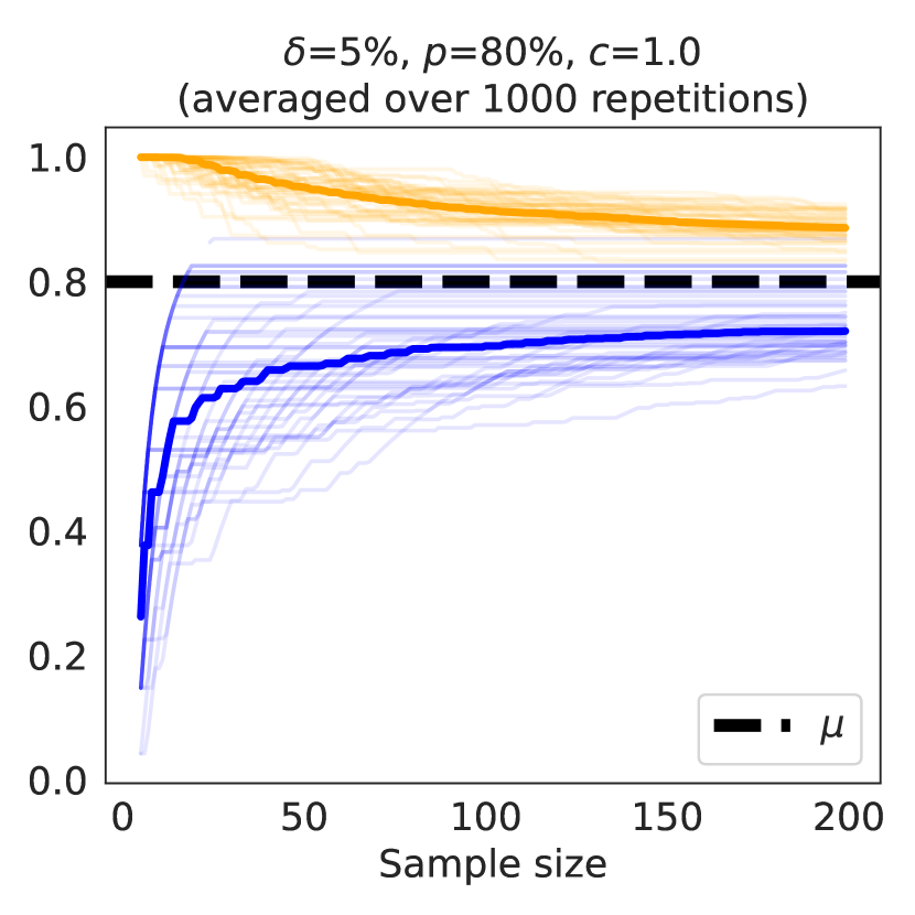
(b) Bernoulli

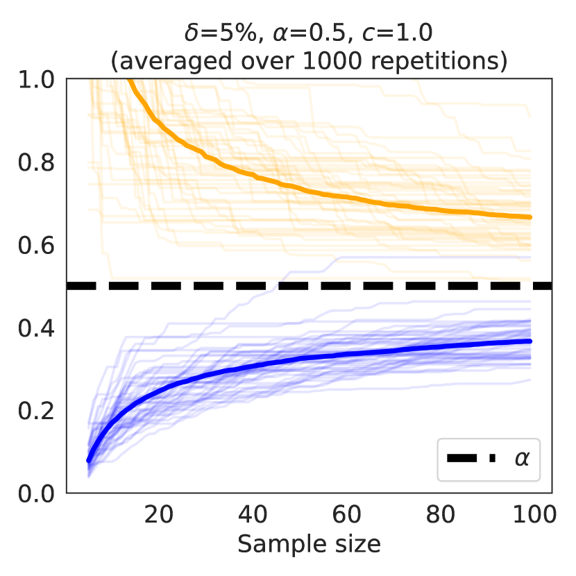
(c) Pareto

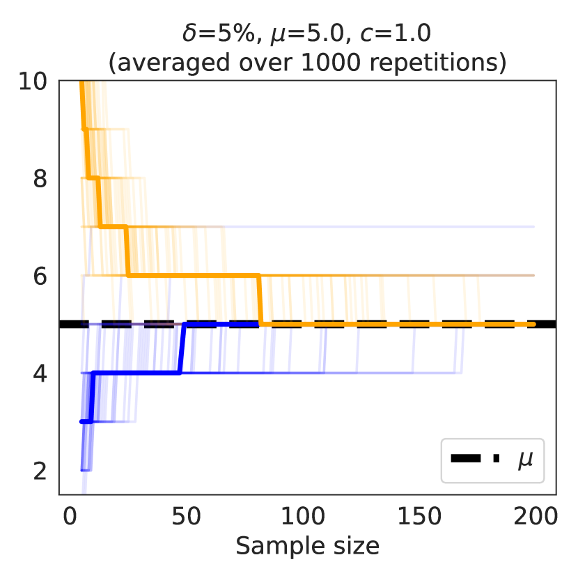
(d) Chi-square

Figure 1: Example of Gaussian time-uniform joint confidence sets for $(\mu,\sigma)=(1,1)$ with sample sizes $n\in\left\{10,25,50,100\right\}$ observations (smaller confidence sets correspond to larger sample sizes), and examples of time-uniform confidence envelopes for $\text{Bernoulli}(0.8)$, $\text{Pareto}(0.5)$ and $\chi^{2}(5)$ on several realizations as a function of the number of observations $n$. Thick lines indicate the median curve over 1000 replicates.

3.3 Proof Sketch: Theorem 3

We now sketch the proof of Theorem 3, and refer the interested reader to the appendix for details.

Step 1: Martingale construction.

For any $\lambda\in\mathbb{R}^{d}$, we introduce the quantity

$$M_{n}^{\lambda} = \exp\left(\langle\lambda,n(\mu_{n}\!-\!\mu)\rangle\!-\!n\mathcal{B}_{\mathcal{L},\theta}(\lambda)\right)\,,$$

where $\mu_{n}\!=\!\frac{1}{n}\sum_{t=1}^{n}\!F(X_{t})$ and $\mu\!=\!\mathbb{E}_{\theta}[F(X)]$. By Lemma 1, $M_{n}^{\lambda}$ is a martingale such that $\mathbb{E}[M_{n}^{\lambda}]\!=\!1$. We now introduce the distribution $q(\theta|\alpha,\beta)=\exp(\langle\theta,\alpha\rangle-\beta\mathcal{L}(\theta))H(\alpha,\beta)$ where $H(\cdot,\cdot)$ is the normalization function, and define the mixture martingale $M_{n}=\int M_{n}^{\lambda}q(\theta+\lambda|\alpha,\beta)d\lambda$. Note that $M_{n}$ also satisfies $\mathbb{E}[M_{n}]=1$.

Step 2. Choice of parameters and duality properties.

Choosing $\alpha=c\nabla\mathcal{L}(\theta)$ and $\beta=c$ yields

$$M_{n}\!=\!G(\theta,c)\!\int\!\!\exp\!\left(\!\langle\lambda,n(\mu_{n}\!-\!\mu)\rangle\!-\!(n\!+\!c)\mathcal{B}_{\mathcal{L},\theta}(\lambda)\!\right)d\lambda\,,$$

where $G(\theta,c)=1/\int\exp\big{(}-c\mathcal{B}_{\mathcal{L}}(\theta^{\prime},\theta)\big{)}d\theta^{\prime}$. Now, we consider the function $\mathcal{B}_{\mathcal{L},\theta}^{\star}(x)=\max_{\lambda}\langle\lambda,x\rangle-\mathcal{B}_{\mathcal{L},\theta}(\lambda)$. Note that its maximal point $\lambda^{\star}_{x}$ satisfies $x+\nabla\mathcal{L}(\theta)=\nabla\mathcal{L}(\theta+\lambda^{\star}_{x})$ for every $x$. In particular, for the choice $x=\frac{n}{n+c}(\mu_{n}-\mu)$, we have $\frac{n}{n+c}\mu_{n}+\frac{c}{n+c}\nabla\mathcal{L}(\theta)=\nabla\mathcal{L}(\theta+\lambda^{\star}_{x})$, which justifies introducing the following regularized estimate

$$\theta_{n,c}(\theta)=(\nabla\mathcal{L})^{-1}\left(\frac{n}{n+c}\mu_{n}+\frac{c}{n+c}\nabla\mathcal{L}(\theta)\right),$$

provided that $\nabla\mathcal{L}$ is one-to-one in $\Theta$.

Step 3. Martingale rewriting and conclusion.

Note that the duality property also yields $\langle\lambda,x\rangle-\mathcal{B}_{\mathcal{L},\theta}(\lambda)-\langle\lambda^{\star}_{x},x\rangle+\mathcal{B}_{\mathcal{L},\theta}(\lambda^{\star}_{x})=\langle\lambda-\lambda^{\star}_{x},\nabla\mathcal{L}(\theta+\lambda^{\star}_{x})\rangle+\mathcal{L}(\theta+\lambda^{\star}_{x})-\mathcal{L}(\theta+\lambda)$ for each $x$. Using this property, we obtain

$$M_{n}=\exp\big{(}(n\!+\!c)\mathcal{B}_{\mathcal{L},\theta}^{\star}(x)\big{)}\frac{G(\theta,c)}{G(\theta_{n,c}(\theta),n+c)}\,.$$

After applying Markov’s inequality, we obtain the following inequality:

$$\mathbb{P}_{\theta}\bigg{[}\mathcal{B}_{\mathcal{L},\theta}^{\star}\bigg{(}\frac{n}{n\!+\!c}(\mu_{n}-\mu)\bigg{)}\geqslant\frac{1}{n\!+\!c}\log\frac{G(\theta_{n,c}(\theta),n\!+\!c)}{\delta\,G(\theta,c)}\bigg{]}\leqslant\delta\,.$$

Now, we use duality property of Bregman divergence to obtain $\mathcal{B}_{\mathcal{L},\theta}^{\star}\!\left(\!\frac{n}{n+c}(\mu_{n}\!-\!\mu)\right)\!=\!\mathcal{B}_{\mathcal{L}}\big{(}\theta,\theta_{n,c}(\theta)\big{)}$, which yields the desired form. Finally, by properties of the martingale $M_{n}$, the deviation bound also holds for any random stopping time $N$, and hence we obtain the time uniform bound by employing a stopping time construction similar to that of Peña et al. (2008); Abbasi-Yadkori et al. (2011).

4 Numerical Experiments

In this section, we provide illustrative numerical results to show the resulting confidence bands built from Theorem 3 are promising alternatives to existing competitors (detailed in Appendix D). All the confidence sets presented here are implemented in the open source concentration-lib Python package (https://pypi.org/project/concentration-lib/).

Comparison.

We compare our confidence envelopes to state-of-the-art time-uniform bounds in Figure 2 and Appendix D. Interestingly, our upper and lower bounds are not necessarily symmetrical, and in the Bernoulli case, they fit within the distribution support without clipping, contrary to most other methods, thus adapting to the local geometry of the family. Our bounds are comparable to those of Kaufmann and Koolen (2021), if slightly tighter; however, we emphasize again that our scope is wider and captures more distributions.

Numerical complexity.

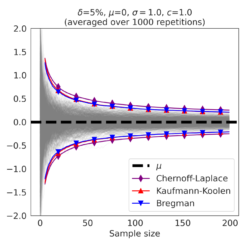
(a) Gaussian

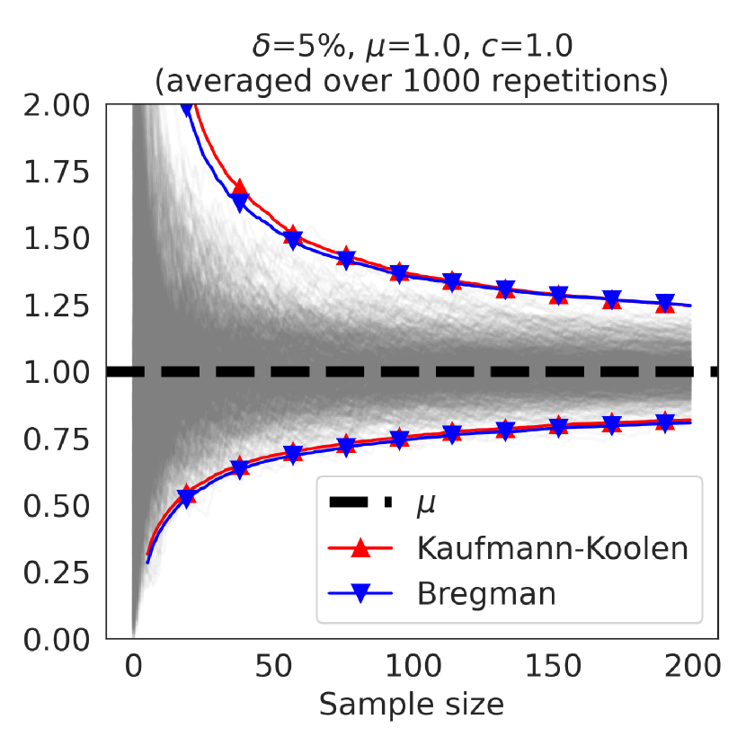
(b) Exponential

(c) Bernoulli

(d) Bernoulli (tuning $c$)

Figure 2: Comparison of median confidence envelopes around the mean for $\mathcal{N}(0,1)$, Bernoulli$(0.8)$ and $\text{Exp}(1)$, as a function of the sample size $n$, over $1000$ independent replicates. Grey lines are trajectories of empirical means $\widehat{\mu}_{n}$. Bottom right: confidence envelopes for varying regularization $c\!\in\![0.1,30]$ for Bernoulli$(0.5)$ distribution. Dotted black line: heuristic $c_{n}\!\approx\!0.12n$.

Some of our formulas (Poisson, Chi-square) require the evaluation of integrals for which no closed-form expression exist. However, these can be estimated up to arbitrary precision by numerical routines, see Remarks 10 and 11 for details. Similarly, the use of special functions (digamma, ratio of Gamma) may lead to numerical instabilities or overflows for large $n$; we recommend instead to use the log-Gamma function and an efficient implementation of the log-sum-exp operator. We report results for $n\!\leqslant\!200$ as we think the small sample regime is where our bounds shine (most reasonable methods produce similar confidence sets for large $n$). Finally, most confidence sets reported in Figure 2 are implicitly defined (after reorganizing terms) as level sets $\{F(\theta)\leqslant 0\}$ for some function $F$. For one-dimensional families, we use a root search routine for a fast estimation of the boundaries of such sets; in higher dimension, we evaluate $F$ on a uniform grid (e.g, in Figure 1(a), we use a $1024\!\times\!1024$ grid over $[\!-\!2,4]\!\times\![0.1,4]$).

Influence of the regularization parameter $c$.

Here, we fix $\delta\!=\!0.05$ (note that all bounds exhibit the typical $\log\frac{1}{\delta}$ dependency). The parameter $c$ is fixed to $c\!=\!1$ and can be interpreted as a number of virtual prior samples, thus introducing a bias. The choice $c\!=\!1$ is a typical value considered in literature on Gaussian concentration. To see the influence of the parameter $c$ on the bounds, we provide a second set of experiments, in which we compute confidence envelopes for $c$ varying between $0.1$ and $30$ (Figure 2(d)). We find that $c$ has limited influence on the width of the confidence interval. To get more insight on the tuning of $c$, we perform additional experiments in Appendix D, where we optimize the confidence width w.r.t. to $c$ for varying sample sizes $n$. The resulting choice $c^{*}_{n}\!=\!\mathop{\mathrm{argmin}}_{c}\lvert\Theta_{n,c}\left(\delta\right)\rvert$ exhibits a linear trend $c^{*}_{n}\!\approx\!0.12n$, which seems consistent across the tested distributions. Of note, the constant $0.12$ is reminiscent of the optimal tuning of the sub-Gaussian Laplace method (Howard et al., 2020). This is consistent with the observation in Section 3.1 that the confidence width $\lvert\Theta_{n,c}\left(\delta\right)\rvert$ is equivalent to the Gaussian confidence width when $n\rightarrow+\infty$. We report in Figure 2(d) this heuristic for $c$. However, we restate that sample a size-dependent regularization parameter $c$ is not supported by the theory (as it would violate the law of iterated logarithms). Now, this does not prevent from choosing a specific horizon of interest $n_{0}$ and set $c\!=\!0.12n_{0}$ to promote sharpness around $n=zn_{0}$.

5 Application: Generalized Likelihood Ratio Test in Exponential Families

In this section, we apply our result to control the false alarm rate of Generalized Likelihood Ratio (GLR) tests when detecting a change of measure from a sequence of observations. The GLR test in the exponential family model $\mathcal{E}$ is defined, for a threshold $\alpha>0$, as

$$\tau(\alpha;\mathcal{E})=\min\{t\in\mathbb{N}:\max_{s\in[0,t)}G^{\mathcal{E}}_{1:s:t}\geqslant\alpha\},$$

where the GLR is defined to be $G^{\mathcal{E}}_{1:s:t}\!=\!\inf_{\theta^{\prime}}\sup_{\theta_{1},\theta_{2}}\log\bigg{(}\!\frac{\prod_{t^{\prime}=1}^{s}p_{\theta_{1}}(X_{t^{\prime}})\!\prod_{t^{\prime}=s+1}^{t}p_{\theta_{2}}(X_{t^{\prime}})}{\prod_{t^{\prime}=1}^{t}p_{\theta^{\prime}}(X_{t^{\prime}})}\!\bigg{)}$.

Hereafter, we consider that all the observations $(X_{t^{\prime}})_{t^{\prime}\in\mathbb{N}}$ come from a distribution with same parameter $\theta\in\Theta$. Then, the false alarm rate of the GLR test can be bounded using

$$\mathbb{P}_{\theta}(\tau(\alpha;\mathcal{E})<\infty)\!=\!\mathbb{P}_{\theta}\big{(}\exists(t,s)\in\mathbb{N}^{2},s<t:G^{\mathcal{E}}_{1:s:t}\geqslant\alpha\big{)}.$$

Observe that solving for the inner supremums in the expression of GLR, we obtain

$$G^{\mathcal{E}}_{1:s:t} = \inf_{\theta^{\prime}}s\mathcal{B}_{\mathcal{L}}(\theta^{\prime},\theta_{1:s})+(t-s)\mathcal{B}_{\mathcal{L}}(\theta^{\prime},\theta_{s+1:t}),$$

where we introduce parameter estimates $\theta_{1:s}$ and $\theta_{s+1:t}$ such that $\nabla\mathcal{L}(\theta_{1:s})=\frac{1}{s}\sum_{t^{\prime}=1}^{s}F(X_{t^{\prime}})$ and $\nabla\mathcal{L}(\theta_{s+1:t})=\frac{1}{t-s}\sum_{t^{\prime}=s+1}^{t}F(X_{t^{\prime}})$, respectively. Hence, the false alarm rate can be controlled as

$$\mathbb{P}_{\theta}(\tau(\alpha;\mathcal{E})\!<\!\infty)\!\leqslant\!\mathbb{P}_{\theta}\Big{(}\!\exists s\!\in\!\mathbb{N}\!:\!s\mathcal{B}_{\mathcal{L}}(\theta,\theta_{1:s})\!\geqslant\!\alpha_{1}\!\Big{)}\!+\!\mathbb{P}_{\theta}\Big{(}\!\exists(t,s)\!\in\!\mathbb{N}^{2},\!s\!<\!t\!:\!(t\!-\!s)\mathcal{B}_{\mathcal{L}}(\theta,\theta_{s+1:t})\!\geqslant\!\alpha_{2}\!\Big{)}$$

for appropriate terms $\alpha_{1},\alpha_{2}$ such that $\alpha=\alpha_{1}+\alpha_{2}$. The control of the first term comes naturally from our time-uniform deviation result (Theorem 3) using a regularized version of the estimate $\theta_{1:s}$. For the second term, we need to study the concentration of $\mathcal{B}_{\mathcal{L}}(\theta,\theta_{s+1:t})$ uniformly over $s$ and $t$.

Doubly time-uniform concentration.

For any $s\!<\!t$, $c>0$ and reference parameter $\theta_{0}\in\Theta$, we define the regularized estimate $\theta_{s+1:t,c}(\theta_{0})=(\nabla\mathcal{L})^{-1}\left(\frac{1}{t-s+c}\left(\sum_{t^{\prime}=s+1}^{t}F(X_{t^{\prime}})+c\nabla\mathcal{L}(\theta_{0})\right)\right)$ built from $(t\!-\!s)$ observations $X_{s+1},\ldots,X_{t}$. Similarly, we introduce the corresponding Bregman information gain $\gamma_{s+1:t,c}(\theta_{0})$ as in Definition 2. The following result extends the Laplace method for exponential families (Theorem 3) to control the Bregman deviation of $\theta_{s+1:t,c}(\theta_{0})$ around $\theta_{0}$.

Theorem 5 (Doubly time-uniform concentration)

Let $\delta\!\in\!(0,1]$ and $g\colon\mathbb{N}\!\rightarrow\!\mathbb{R}_{+}^{*}$ such that $\sum_{t=1}^{\infty}1/g(t)\!\leqslant\!1$ (e.g., $g(t)\!=\!\kappa(1\!+\!t)\log^{2}(1\!+\!t)$ where $\kappa=2.10975$). Then, under the assumptions of Definition 2, it holds that

$$\mathbb{P}_{\theta}\!\left[\exists t\in\mathbb{N},\exists s\!<\!t:\!(t\!-\!s\!+\!c)\mathcal{B}_{\mathcal{L}}(\theta,\theta_{s+1:t,c}(\theta))\!\geqslant\!\log\frac{g(t)}{\delta}+\gamma_{s+1:t,c}(\theta)\right]\leqslant\delta\,.$$

Remark 6

Maillard (2019a) proves a doubly uniform concentration inequality for means of (sub)-Gaussian random variables and conjectures that it could be extended to other types of changes, such as changes of variance in a Gaussian family. Theorem 5 can be seen as a generalization of this result to generic exponential families. This naturally comes with additional challenges due to the intrinsic local geometry of exponential families. The proof of this result is deferred to Appendix E.

A regularized GLR test.

For a given false alarm (i.e., false positive) probability $\delta\in(0,1]$ and parameter $c>0$, we define the regularized GLR test $\tau^{\delta}_{c}(\mathcal{E})$ as follows:

$$\Theta_{s,c}(\delta)=\left\{\theta\in\Theta:(s+c)\mathcal{B}_{\mathcal{L}}(\theta,\theta_{1:s,c}(\theta))\leqslant\log(1/\delta)+\gamma_{1:s,c}(\theta)\right\}\,,$$

$$\Theta_{s+1:t,c}(\delta)=\left\{\theta\in\Theta:(t-s+c)\mathcal{B}_{\mathcal{L}}(\theta,\theta_{s+1:t,c}(\theta))\leqslant\log(g(t)/\delta)+\gamma_{s+1:t,c}(\theta)\right\}\,,$$

$$\tau^{\delta}_{c}(\mathcal{E})=\min\left\{t\in\mathbb{N}:\exists s<t,\Theta_{s,c}(\delta/2)\cap\Theta_{s+1:t,c}(\delta/2)=\emptyset\right\}\,.$$

Note that, under the measure $\mathbb{P}_{\theta}$, $\theta\in\Theta_{s,c}(\delta/2)$ holds with probability at least $1-\delta/2$ by time-uniform concentration over $s$ (Theorem 3), and $\theta\in\Theta_{s+1:t,c}(\delta/2)$ holds with probability at least $1\!-\!\delta/2$ by doubly time-uniform concentration over both $s$ and $t$ (Theorem 5). Then, by a union-bound, this test is guaranteed to have a false alarm probability controlled by $\delta$. The factor $g(t)$ is essentially a function growing slightly faster than linearly; other common choices include $g(t)\propto t^{\eta}$ for some $\eta>1$, though it leads to a looser bound due to the faster growth. Furthermore, if one is interested in detecting changes up to a known horizon $T$, one can replace the function $g(t)$ by the slightly tighter factor $g(t)=\kappa(1\!+\!t)\log^{2}(1\!+\!t)$ with $\kappa\!=\!\sum_{t=1}^{T}1/g(t)$ and still guarantee a false alarm rate under $\delta$. In Appendix E.3, we report simulations of this GLR test to detect changes of variance in the family of centered Gaussian (Figure 14), which answers an open question from Maillard (2019a).

6 Conclusion

We apply the method of mixture to derive a time-uniform deviation inequality for generic parametric exponential families expressed in terms of their Bregman divergences, highlighting the role of a quantity, the Bregman information gain, that is related to the geometry of the family. We specialize this general result to build confidence sets for classical examples. Our method compares favorably to the state-of-the art for Gaussian, Bernoulli and exponential distributions, and extends to other families like Chi-square, Pareto and two-parameter Gaussian, where no known time-uniform bound exists. Our method is also general enough to design GLR tests for change detection. An interesting direction for future work would be to consider the case where the log-partition function (and thus the Bregman divergence) is misspecified or unknown and has to be learned alongside the parameter.

The authors acknowledge the funding of the French National Research Agency, the French Ministry of Higher Education and Research, Inria, the MEL and the I-Site ULNE regarding project R-PILOTE-19-004-APPRENF and Bandits For Health (B4H). We thank the anonymous reviewers for their careful reading of the paper and their suggestions for improvements. Experiments presented in this paper were carried out using the Grid’5000 testbed, supported by a scientific interest group hosted by Inria and including CNRS, RENATER and several universities as well as other organizations (see https://www.grid5000.fr).

Appendix A Proof of the Main Result About Bregman Deviations

In this section, we detail the proof of the main results regarding Bregman deviation inequalities, stated with its two variants Theorem 3 and 7, We start in Section A.1 with the proof of Theorem 3 when considering a numerical constant $c$ to build the regularizer. In Section A.2, we then provide the proof for Theorem 7 when considering instead a Legendre function $\mathcal{L}_{0}$ as a regularizer, and also extend to the non i.i.d. case.

A.1 Proof of Bregman concentration using mixture parameter $c$

The proof of this first result follows an adaptation of the method of mixture, combined with properties of Bregman divergences recalled in Lemma 1.

See 3

Proof of Theorem 3:

Step 1. Martingale and mixture martingale construction.

Let us note that $\mathbb{E}_{\theta}[F(X)]=\nabla\mathcal{L}(\theta)$ and $\log\mathbb{E}_{\theta}\left[\exp\langle\lambda,F(X)\rangle\right]=\mathcal{L}(\theta+\lambda)-\mathcal{L}(\theta)$. Hence, we deduce that

$$\log\mathbb{E}_{\theta}\left[\exp\langle\lambda,F(X)-\mathbb{E}_{\theta}[F(X)]\rangle\right]=\mathcal{B}_{\mathcal{L},\theta}(\lambda)\stackrel{{\scriptstyle\rm def}}{{=}}\mathcal{L}(\theta+\lambda)-\mathcal{L}(\theta)-\langle\lambda,\nabla\mathcal{L}(\theta)\rangle\,.$$

Now, let $\mu_{n}=\frac{1}{n}\sum_{t=1}^{n}F(X_{t})$ and $\mu=\mathbb{E}_{\theta}[F(X)]$. For any $\lambda\in\mathbb{R}^{d}$, the following quantity

$$M_{n}^{\lambda} = \exp\bigg{(}\langle\lambda,n(\mu_{n}-\mu)\rangle-n\mathcal{B}_{\mathcal{L},\theta}(\lambda)\bigg{)}\,,$$

is thus a martingale such that $\mathbb{E}[M_{n}^{\lambda}]=1$.

We now introduce the distribution $q(\theta|\alpha,\beta)=H(\alpha,\beta)\cdot\exp(\langle\theta,\alpha\rangle-\beta\mathcal{L}(\theta))$ where $H$ is the normalization term. We further introduce the following quantity

$$M_{n}=\int_{\Lambda_{\theta}}M_{n}^{\lambda}q(\theta+\lambda|\alpha,\beta)d\lambda\,,$$

where $\Lambda_{\theta}=\{\lambda:\theta+\lambda\in\Theta\}$. This also satisfies $\mathbb{E}[M_{n}]=1$. Further, we have the rewriting

$$M_{n}=H(\alpha,\beta)\int_{\Lambda_{\theta}}\exp\bigg{(}\langle\lambda,n(\mu_{n}-\mu)\rangle-n\mathcal{B}_{\mathcal{L},\theta}(\lambda)+\langle\lambda+\theta,\alpha\rangle-\beta\mathcal{L}(\theta+\lambda)\bigg{)}d\lambda\,.$$

Step 2. Choice of parameters and duality properties. Considering in particular the choice $\alpha=c\nabla\mathcal{L}(\theta)$ and $\beta=c$, we get

$$M_{n} = H(c\nabla\mathcal{L}(\theta),c)\int_{\Lambda_{\theta}}\exp\bigg{(}\langle\lambda,n(\mu_{n}-\mu)\rangle-n\mathcal{B}_{\mathcal{L},\theta}(\lambda)+c\langle\lambda+\theta,\nabla\mathcal{L}(\theta)\rangle-c\mathcal{L}(\theta+\lambda)\bigg{)}d\lambda$$

$$= G(\theta,c)\int_{\Lambda_{\theta}}\exp\bigg{(}\langle\lambda,n(\mu_{n}-\mu)\rangle-(n+c)\mathcal{B}_{\mathcal{L},\theta}(\lambda)\bigg{)}d\lambda~{},$$

where we introduce the following quantity

$$G(\theta,c)=H(c\nabla\mathcal{L}(\theta),c)\exp\bigg{(}c\langle\theta,\nabla\mathcal{L}(\theta)\rangle-c\mathcal{L}(\theta)\bigg{)} = \frac{\exp\bigg{(}c\langle\theta,\nabla\mathcal{L}(\theta)\rangle-c\mathcal{L}(\theta)\bigg{)}}{\int_{\Theta}\exp\bigg{(}c\langle\theta^{\prime},\nabla\mathcal{L}(\theta)\rangle-c\mathcal{L}(\theta^{\prime})\bigg{)}d\theta^{\prime}}$$

$$= \bigg{[}\int_{\Theta}\exp\big{(}-c\mathcal{B}_{\mathcal{L}}(\theta^{\prime},\theta)\big{)}d\theta^{\prime}\bigg{]}^{-1}~{}.$$

At this point, let us introduce $x=\frac{n}{n+c}(\mu_{n}-\mu)$. We also consider the Legendre-Fenchel dual function $\mathcal{B}_{\mathcal{L},\theta}^{\star}(x)=\max_{\lambda}\langle\lambda,x\rangle-\mathcal{B}_{\mathcal{L},\theta}(\lambda)$ and denote $\lambda^{\star}_{x}$ its maximal point. Now, we note that $x+\nabla\mathcal{L}(\theta)=\nabla\mathcal{L}(\theta+\lambda^{\star}_{x})$ and thus

$$\langle\lambda,x\rangle-\mathcal{B}_{\mathcal{L},\theta}(\lambda)-\langle\lambda^{\star}_{x},x\rangle+\mathcal{B}_{\mathcal{L},\theta}(\lambda^{\star}_{x}) = \langle\lambda-\lambda^{\star}_{x},x+\nabla\mathcal{L}(\theta)\rangle+\mathcal{L}(\theta+\lambda^{\star}_{x})-\mathcal{L}(\theta+\lambda)$$

$$= \langle\lambda-\lambda^{\star}_{x},\nabla\mathcal{L}(\theta+\lambda^{\star}_{x})\rangle+\mathcal{L}(\theta+\lambda^{\star}_{x})-\mathcal{L}(\theta+\lambda)\,.$$

Also, since it holds that $x=\frac{n}{n+c}(\mu_{n}-\nabla\mathcal{L}(\theta))$, then the quantity $x+\nabla\mathcal{L}(\theta)=\nabla\mathcal{L}(\theta+\lambda^{\star}_{x})$ rewrites $\frac{n}{n+c}\mu_{n}+\frac{c}{n+c}\nabla\mathcal{L}(\theta)=\nabla\mathcal{L}(\theta+\lambda^{\star}_{x})$, which justifies to introduce the following regularized parameter estimate

$$\theta_{n,c}(\theta)=(\nabla\mathcal{L})^{-1}\bigg{(}\frac{n}{n+c}\mu_{n}+\frac{c}{n+c}\nabla\mathcal{L}(\theta)\bigg{)}\,.$$

Step 3. Martingale rewriting and conclusion. Using this property, we note that

$$M_{n} = \exp\big{(}(n\!+\!c)\mathcal{B}_{\mathcal{L},\theta}^{\star}(x)\big{)}\cdot G(\theta,c)\!\!\int_{\Lambda_{\theta}}\!\!\exp\!\bigg{(}\!(n\!+\!c)\Big{[}\langle\lambda\!-\!\lambda^{\star}_{x},\nabla\mathcal{L}(\theta\!+\!\lambda^{\star}_{x})\rangle\!-\!\mathcal{L}(\theta\!+\!\lambda)\!+\!\mathcal{L}(\theta\!+\!\lambda^{\star}_{x})\Big{]}\!\bigg{)}d\lambda$$

$$= \exp\big{(}(n\!+\!c)\mathcal{B}_{\mathcal{L},\theta}^{\star}(x)\big{)}\cdot G(\theta,c)\!\int_{\Lambda_{\theta}}\!\exp\!\bigg{(}\langle\lambda\!+\!\theta,(n\!+\!c)\nabla\mathcal{L}(\theta\!+\!\lambda^{\star}_{x})\rangle\!-\!(n\!+\!c)\mathcal{L}(\theta\!+\!\lambda)\bigg{)}d\lambda\times$$

$$\exp\bigg{(}\!-(n\!+\!c)\langle\lambda^{\star}_{x}\!+\!\theta,\nabla\mathcal{L}(\theta\!+\!\lambda^{\star}_{x})+(n\!+\!c)\mathcal{L}(\theta\!+\!\lambda^{\star}_{x})\rangle\bigg{)}$$

$$= \exp\big{(}(n\!+\!c)\mathcal{B}_{\mathcal{L},\theta}^{\star}(x)\big{)}\frac{G(\theta,c)}{G(\theta+\lambda^{\star}_{x},n+c)}=\exp\big{(}(n\!+\!c)\mathcal{B}_{\mathcal{L},\theta}^{\star}(x)\big{)}\frac{G(\theta,c)}{G(\theta_{n,c}(\theta),n+c)}\,.$$

We then apply simple Markov inequality, which yields for all constant $c$,

$$\forall\delta\in(0,1],\quad\mathbb{P}\bigg{(}\mathcal{B}_{\mathcal{L},\theta}^{\star}\bigg{(}\frac{n}{n\!+\!c}(\mu_{n}\!-\!\mu)\bigg{)}\geqslant\frac{1}{n+c}\log\bigg{(}\frac{G(\theta_{n,c}(\theta),n+c)}{G(\theta,c)}\frac{1}{\delta}\bigg{)}\bigg{)}\leqslant\delta.$$

To conclude, we use the duality property of the Bregman divergence (Lemma 1), considering that $\nabla\mathcal{L}$ is invertible. Indeed, denoting $\alpha=n/(n+c)$, and $\theta_{n}=(\nabla\mathcal{L})^{-1}(\mu_{n})$, it comes

$$\mathcal{B}_{\mathcal{L},\theta}^{\star}\bigg{(}\alpha(\mu_{n}-\mu)\bigg{)}=\mathcal{B}_{\mathcal{L}}\big{(}\theta,\theta_{\alpha}\big{)}\,\qquad\text{where}\,\,\theta_{\alpha}=\nabla\mathcal{L}^{-1}\big{(}\alpha\nabla\mathcal{L}(\theta_{n})+(1-\alpha)\nabla\mathcal{L}(\theta)\big{)}=\theta_{n,c}(\theta)\,.$$

Last, we note that this extends from a single $n$ to being time-uniform thanks to Doob’s maximal inequality for nonnegative supermartingale applied to $M_{n}$ (also known as Vile’s inequality Ville (1939)). $\hfill\square$

A.2 Bregman concentration using Legendre function $\mathcal{L}_{0}$

In this section, we state a more general result that can handle the case of sequence $(X_{t})_{t\geqslant 1}$ of random variables that are not independent, each having possibly different distribution from others.

Theorem 7 (Laplace method for non i.i.d. samples)

Suppose $\{\mathcal{H}_{t}\}_{t=0}^{\infty}$ is a filtration such that for each $t\geqslant 1$, (i) $X_{t}$ is $\mathcal{H}_{t}$-measurable, (ii) $F_{t}$ and $h_{t}$ are $\mathcal{H}_{t-1}$-measurable and (iii) given $\mathcal{H}_{t-1}$, $X_{t}\sim p_{\theta_{0},t}$ where $p_{\theta_{0},t}$ belongs to an exponential family with parameter $\theta_{0}$, feature function $F_{t}$ and base function $h_{t}$. Let $\mathcal{L}_{t}$ be the log-partition function corresponding to $F_{t}$. For any Legendre (i.e., strictly convex and continuously differentiable) function $\mathcal{L}_{0}:\Theta\to\mathbb{R}$ such that $\exp(-\mathcal{L}_{0})$ is integrable and any $n\in\mathbb{N}$, we introduce the parameter estimate and Bregman information gain

$$\theta_{n,\mathcal{L}_{0}} =\Big{(}\sum_{t=0}^{n}\nabla\mathcal{L}_{t}\Big{)}^{-1}\Big{(}\sum_{t=1}^{n}F_{t}(X_{t})\Big{)}\,,$$

$$\gamma_{n,\mathcal{L}_{0}} =\log\bigg{(}\frac{\int_{\Theta}\exp\Big{(}-\mathcal{L}_{0}(\theta^{\prime})\Big{)}d\theta^{\prime}}{\int_{\Theta}\exp\Big{(}-\sum_{t=0}^{n}\mathcal{B}_{\mathcal{L}_{t}}(\theta^{\prime},\theta_{n,\mathcal{L}_{0}})\Big{)}d\theta^{\prime}}\bigg{)}\,,$$

and then, for any $\delta\in(0,1]$, the set

$$\Theta_{n,\mathcal{L}_{0}}(\delta)=\left\{\theta:\sum_{t=0}^{n}\mathcal{B}_{\mathcal{L}_{t}}\left(\theta,\theta_{n,\mathcal{L}_{0}}\right)-\mathcal{L}_{0}(\theta)\leqslant\log\frac{1}{\delta}+\gamma_{n,\mathcal{L}_{0}}\right\}\,.$$

Then, the following time-uniform concentration holds:

$$\mathbb{P}\big{[}\exists n\in\mathbb{N}:\theta_{0}\notin\Theta_{n,\mathcal{L}_{0}}(\delta)\big{]}\leqslant\delta\,.$$

In contrast to Theorem 3 that involves a local regularization using the true parameter $\theta_{0}\in\Theta$ of the family and a constant $c\!>\!0$, here we make use of a global regularization, in the form of the Legendre function $\mathcal{L}_{0}$. Concretely, the regularized parameter estimate $\theta_{n,\mathcal{L}_{0}}$ and the Bregman information gain $\gamma_{n,\mathcal{L}_{0}}$ do not depend on the true parameter $\theta_{0}$, thus making for a more explicit confidence set $\Theta_{n,\mathcal{L}_{0}}$. The trade-off here is that the choice of regularizer is limited by the integrability assumption on $\exp(-\mathcal{L}_{0})$, which is critical to build an appropriate prior for the method of mixtures.

The proof of this result follows a similar line of proof as before. However the use of $\mathcal{L}_{0}$ instead of $c$ induces a few changes that we detail below. In particular, we use a different prior to build the mixture of martingales.

Proof of Theorem 7:

Step 1. Martingale and mixture martingale construction. For any $\lambda\in\mathbb{R}^{d}$, we define

$$M_{n}^{\lambda}=\exp\left(\sum_{t=1}^{n}\left(\lambda^{\top}\left(F_{t}(X_{t})-\mathbb{E}_{\theta}\left[F_{t}(X_{t})\right]\right)-B_{\mathcal{L}_{t},\theta}(\lambda)\right)\right)~{},$$

where we introduced $B_{\mathcal{L}_{t},\theta}(\lambda)=\mathcal{L}_{t}(\theta+\lambda)-\mathcal{L}_{t}(\theta)-\langle\lambda,\nabla\mathcal{L}_{t}(\theta)\rangle$ for convenience.

Note that $M_{n}^{\lambda}>0$ and

$$\mathbb{E}_{\theta}\left[\exp\left(\lambda^{\top}F_{t}(X_{t})\right)\right] =\exp\left(\mathcal{L}_{t}(\theta+\lambda)-\mathcal{L}_{t}(\theta)\right)~{},$$

$$\mathbb{E}_{\theta}\left[\exp\left(\lambda^{\top}\mathbb{E}_{\theta}[F_{t}(X_{t})\right)\right] =\exp\left(\lambda^{\top}\mathcal{L}_{t}(\theta)\right)~{}.$$

Note that $M_{n}^{\lambda}$ is $\mathcal{H}_{n}$-measurable and in fact $\mathbb{E}[M_{n}^{\lambda}|\mathcal{H}_{n-1}]=M_{n-1}^{\lambda}$. Therefore $\{M_{n}^{\lambda}\}_{n=0}^{\infty}$ is a nonnegative martingale adapted to the filtration $\{\mathcal{H}_{n}\}_{n=0}^{\infty}$ and actually satisfies $\mathbb{E}\left[M_{n}^{\lambda}\right]=1~{}$. For any prior density $q(\theta)$ for $\theta$, we now define a mixture of martingales

$$M_{n}=\int_{\Lambda_{\theta}}M_{n}^{\lambda}q(\theta+\lambda)d\lambda~{}.$$ (1)

where $\Lambda_{\theta}=\{\lambda:\theta+\lambda\in\Theta\}$. Then $M_{n}$ is also a martingale and actually satisfies $\mathbb{E}\left[M_{n}\right]=1~{}$. Now consider the prior density

$$q(\theta+\lambda)=c_{0}\cdot\exp\left(-\mathcal{L}_{0}(\theta+\lambda)\right)~{},$$ (2)

where $c_{0}=\frac{1}{\int_{\Theta}\exp\left(-\mathcal{L}_{0}(\theta^{\prime})\right)d\theta^{\prime}}$ (which is well-defined since $\exp(-\mathcal{L}_{0})$ is integrable over $\Theta$). We then have

$$M_{n}=c_{0}\int_{\Lambda_{\theta}}\exp\left(\lambda^{\top}S_{n}-\sum_{t=1}^{n}\mathcal{B}_{\mathcal{L}_{t},\theta}(\lambda)-\mathcal{L}_{0}(\theta+\lambda)\right)d\lambda~{},$$

where we denote $S_{n}=\sum_{t=1}^{n}\left(F_{t}(X_{t})-\mathbb{E}_{\theta}\left[F_{t}(X_{t})\right]\right)$. Now, from the formula of parameter estimate, we have

$$\quad\sum_{t=1}^{n}\nabla\mathcal{L}_{t}(\theta_{n,\mathcal{L}_{0}})+\nabla\mathcal{L}_{0}(\theta_{n,\mathcal{L}_{0}})=\sum_{t=1}^{n}F_{t}(X_{t})~{}.$$ (3)

This yields $S_{n}=\sum_{t=1}^{n}\left(\nabla\mathcal{L}_{t}(\theta_{n,\mathcal{L}_{0}})-\nabla\mathcal{L}_{t}(\theta)\right)+\nabla\mathcal{L}_{0}(\theta_{n,\mathcal{L}_{0}})$.

Step 2. Legendre function and Bregman properties. We now introduce the function $\mathcal{L}_{1:n}(\theta)=\sum_{t=1}^{n}\mathcal{L}_{t}(\theta)$. Note that $\mathcal{L}_{1:n}$ is a also Legendre function and its associated Bregman divergence satisfies

$$\mathcal{B}_{\mathcal{L}_{1:n}}(\theta^{\prime},\theta)=\sum_{t=1}^{n}\left(\mathcal{L}_{t}(\theta^{\prime})-\mathcal{L}_{t}(\theta)-(\theta^{\prime}-\theta)^{\top}\nabla\mathcal{L}_{t}(\theta)\right)=\sum_{t=1}^{n}\mathcal{B}_{\mathcal{L}_{t}}(\theta^{\prime},\theta).$$

In this notation, we can rewrite $\sum_{t=1}^{n}\mathcal{B}_{\mathcal{L}_{t},\theta}(\lambda)=\mathcal{B}_{\mathcal{L}_{1:n},\theta}(\lambda)$ and $S_{n}=\nabla\mathcal{L}_{n}(\theta_{n,\mathcal{L}_{0}})-\nabla\mathcal{L}_{n}(\theta)+\nabla\mathcal{L}_{0}(\theta_{n,\mathcal{L}_{0}})$. We then obtain

$$M_{n}=c_{0}\cdot\exp\left(-\mathcal{L}_{0}(\theta)\right)\int_{\Lambda_{\theta}}\exp\left(\lambda^{\top}x_{n}-\mathcal{B}_{\mathcal{L}_{1:n},\theta}(\lambda)+\lambda^{\top}x_{0}-\mathcal{B}_{\mathcal{L}_{0},\theta}(\lambda)\right)d\lambda~{},$$ (4)

where we have introduced $x_{0}=\nabla\mathcal{L}_{0}(\theta_{n,\mathcal{L}_{0}})-\nabla\mathcal{L}_{0}(\theta)$ and $x_{n}=\nabla\mathcal{L}_{1:n}(\theta_{n,\mathcal{L}_{0}})-\nabla\mathcal{L}_{1:n}(\theta)$.

We now have from the Bregman-duality property recalled in Lemma 1 that

$$\sup_{\lambda\in\mathbb{R}^{d}}\left(\lambda^{\top}x_{n}-\mathcal{B}_{\mathcal{L}_{1:n},\theta}(\lambda)\right) =\mathcal{B}_{\mathcal{L}_{1:n},\theta}^{\star}(x_{n})$$

$$=\mathcal{B}_{\mathcal{L}_{1:n},\theta}^{\star}(\nabla\mathcal{L}_{1:n}(\theta_{n,\mathcal{L}_{0}})-\nabla\mathcal{L}_{1:n}(\theta))=\mathcal{B}_{\mathcal{L}_{1:n}}(\theta,\theta_{n,\mathcal{L}_{0}})~{}.$$

Further, any optimal $\lambda$ must satisfy

$$\nabla\mathcal{L}_{1:n}(\theta+\lambda)-\nabla\mathcal{L}_{1:n}(\theta)=x_{n}\implies\nabla\mathcal{L}_{1:n}(\theta+\lambda)=\nabla\mathcal{L}_{1:n}(\theta_{n,\mathcal{L}_{0}})~{}.$$

One possible solution is $\lambda^{\star}=\theta_{n,\mathcal{L}_{0}}-\theta$. We then have

$$\lambda^{\top}x_{n}-\mathcal{B}_{\mathcal{L}_{1:n},\theta}(\lambda)$$

$$=\lambda^{\top}x_{n}-\mathcal{B}_{\mathcal{L}_{1:n},\theta}(\lambda)+\mathcal{B}_{\mathcal{L}_{1:n}}(\theta,\theta_{n,\mathcal{L}_{0}})-\left({\lambda^{\star}}^{\top}x_{n}-\mathcal{B}_{\mathcal{L}_{1:n},\theta}(\lambda^{\star})\right)$$

$$=\mathcal{B}_{\mathcal{L}_{1:n}}(\theta,\theta_{n,\mathcal{L}_{0}})+(\lambda-\lambda^{\star})^{\top}\nabla\mathcal{L}_{n}(\theta+\lambda^{\star})+\mathcal{B}_{\mathcal{L}_{1:n},\theta}(\lambda^{\star})-\mathcal{B}_{\mathcal{L}_{1:n},\theta}(\lambda)-(\lambda-\lambda^{\star})^{\top}\nabla\mathcal{L}_{1:n}(\theta)$$

$$=\mathcal{B}_{\mathcal{L}_{1:n}}(\theta,\theta_{n,\mathcal{L}_{0}})+(\lambda-\lambda^{\star})^{\top}\nabla\mathcal{L}_{1:n}(\theta+\lambda^{\star})+\mathcal{L}_{1:n}(\theta+\lambda^{\star})-\mathcal{L}_{1:n}(\theta+\lambda)~{}.$$ (5)

Similarly, we have

$$\lambda^{\top}x_{0}-\mathcal{B}_{\mathcal{L}_{0},\theta}(\lambda)=\mathcal{B}_{\mathcal{L}_{0}}(\theta,\theta_{n,\mathcal{L}_{0}})+(\lambda-\lambda^{\star})^{\top}\nabla\mathcal{L}_{0}(\theta+\lambda^{\star})+\mathcal{L}_{0}(\theta+\lambda^{\star})-\mathcal{L}_{0}(\theta+\lambda)\,.$$ (6)

Step 3. Martingale rewriting and conclusion. Plugin-in (6) and (5) in (4), we now obtain

$$M_{n} =c_{0}\exp\Big{(}\sum_{j\in\{0,1:n\}}\mathcal{B}_{\mathcal{L}_{j}}(\theta,\theta_{n,\mathcal{L}_{0}})-\mathcal{L}_{0}(\theta)\Big{)}$$

$$\quad\quad\times\int_{\Lambda_{\theta}}\exp\Big{(}\sum_{j\in\{0,1:n\}}\left((\lambda-\lambda^{\star})^{\top}\nabla\mathcal{L}_{j}(\theta+\lambda^{\star})+\mathcal{L}_{j}(\theta+\lambda^{\star})-\mathcal{L}_{j}(\theta+\lambda)\right)\Big{)}d\lambda$$

$$=c_{0}\exp\Big{(}\sum_{j\in\{0,1:n\}}\mathcal{B}_{\mathcal{L}_{j}}(\theta,\theta_{n,\mathcal{L}_{0}})-\mathcal{L}_{0}(\theta)\Big{)}\cdot\exp\Big{(}-\sum_{j\in\{0,1:n\}}\left((\theta+\lambda^{\star})^{\top}\nabla\mathcal{L}_{j}(\theta+\lambda^{\star})-\mathcal{L}_{j}(\theta+\lambda^{\star})\right)\Big{)}$$

$$\quad\quad\times\int_{\Lambda_{\theta}}\exp\Big{(}\sum_{j\in\{0,1:n\}}\left((\theta+\lambda)^{\top}\nabla\mathcal{L}_{j}(\theta+\lambda^{\star})-\mathcal{L}_{j}(\theta+\lambda)\right)\Big{)}d\lambda$$

$$=\frac{c_{0}}{c_{n}}\exp\Big{(}\sum_{j\in\{0,1:n\}}\mathcal{B}_{\mathcal{L}_{j}}(\theta,\theta_{n,\mathcal{L}_{0}})-\mathcal{L}_{0}(\theta)\Big{)}$$

$$\quad\quad\times\frac{\int_{\Lambda_{\theta}}\exp\left(\sum_{j\in\{0,1:n\}}\left((\theta+\lambda)^{\top}\nabla\mathcal{L}_{j}(\theta+\lambda^{\star})-\mathcal{L}_{j}(\theta+\lambda)\right)\right)d\lambda}{\int_{\Theta}\exp\left(\sum_{j\in\{0,1:n\}}\left((\theta^{\prime})^{\top}\nabla\mathcal{L}_{j}(\theta+\lambda^{\star})-\mathcal{L}_{j}(\theta^{\prime})\right)\right)d\theta^{\prime}}$$

$$=\frac{c_{0}}{c_{n}}\exp\Big{(}\sum_{t=1}^{n}\mathcal{B}_{\mathcal{L}_{t}}(\theta,\theta_{n,\mathcal{L}_{0}})+\mathcal{B}_{\mathcal{L}_{0}}(\theta,\theta_{n,\mathcal{L}_{0}})-\mathcal{L}_{0}(\theta)\Big{)}~{},$$

where we have introduced $c_{n}=\frac{\exp\left(\sum_{j\in\{0,1:n\}}\left((\theta+\lambda^{\star})^{\top}\nabla\mathcal{L}_{j}(\theta+\lambda^{\star})-\mathcal{L}_{j}(\theta+\lambda^{\star})\right)\right)}{\int_{\Theta}\exp\left(\sum_{j\in\{0,1:n\}}\left((\theta^{\prime})^{\top}\nabla\mathcal{L}_{j}(\theta+\lambda^{\star})-\mathcal{L}_{j}(\theta^{\prime})\right)\right)d\theta^{\prime}}~{}.$

We then obtain the following result by a simple application of Markov’s inequality, which yields

$$\mathbb{P}\left[\sum_{t=1}^{n}\mathcal{B}_{\mathcal{L}_{t}}(\theta,\theta_{n,\mathcal{L}_{0}})+\mathcal{B}_{\mathcal{L}_{0}}(\theta,\theta_{n,\mathcal{L}_{0}})-\mathcal{L}_{0}(\theta)\geqslant\log\left(\frac{c_{n}}{c_{0}}\frac{1}{\delta}\right)\right]$$

$$=\mathbb{P}\left[M_{n}\geqslant\frac{1}{\delta}\right]\leqslant\delta\cdot\mathbb{E}\left[M_{n}\right]=\delta~{}.$$ (7)

Finally, since $\lambda^{\star}=\theta_{n,\mathcal{L}_{0}}-\theta$, we have the more explicit form

$$\frac{c_{n}}{c_{0}} =\frac{\int_{\Theta}\exp\Big{(}-\mathcal{L}_{0}(\theta^{\prime})\Big{)}d\theta^{\prime}}{\int_{\Theta}\exp\Big{(}-\sum\limits_{j\in\{0,1:n\}}\mathcal{B}_{\mathcal{L}_{j}}(\theta^{\prime},\theta+\lambda^{\star})\Big{)}d\theta^{\prime}}$$

$$=\frac{\int_{\Theta}\exp\Big{(}-\mathcal{L}_{0}(\theta^{\prime})\Big{)}d\theta^{\prime}}{\int_{\Theta}\exp\Big{(}-\sum_{t=1}^{n}\mathcal{B}_{\mathcal{L}_{t}}(\theta^{\prime},\theta_{n,\mathcal{L}_{0}})-\mathcal{B}_{\mathcal{L}_{0}}(\theta^{\prime},\theta_{n,\mathcal{L}_{0}})\Big{)}d\theta^{\prime}}~{}.$$

We obtain the time-uniform bound by applying Doob’s maximal inequality for nonnegative supermartingale. $\hfill\square$

The general result of Theorem 7 specifies straightforwardly to the case when all observations have same law, yielding the following corollary that we state now for completeness.

Corollary 8

Let $\mu_{n}=\frac{1}{n}\sum_{t=1}^{n}F(X_{t})$. For all Legendre function $\mathcal{L}_{0}$ such that $\exp(-\mathcal{L}_{0})$ is integrable over $\Theta$, let

$$\theta_{n,\mathcal{L}_{0}}\!=\big{(}\nabla\mathcal{L}\!+\!\frac{1}{n}\nabla\mathcal{L}_{0}\big{)}^{-1}(\mu_{n})\,\text{ and }\,\gamma_{n,\mathcal{L}_{0}}\!=\log\left(\frac{\int_{\Theta}\exp\Big{(}-\mathcal{L}_{0}(\theta^{\prime})\Big{)}d\theta^{\prime}}{\int_{\Theta}\exp\Big{(}-\!n\mathcal{B}_{\mathcal{L}}\left(\theta^{\prime},\theta_{n,\mathcal{L}_{0}}\right)\!-\!\mathcal{B}_{\mathcal{L}_{0}}\left(\theta^{\prime},\theta_{n,\mathcal{L}_{0}}\right)\Big{)}d\theta^{\prime}}\right)\,.$$

Then for all $\delta\in(0,1],$

$$\mathbb{P}\bigg{(}\exists n\in\mathbb{N},\,\,n\mathcal{B}_{\mathcal{L}}\left(\theta,\theta_{n,\mathcal{L}_{0}}\right)+\mathcal{B}_{\mathcal{L}_{0}}\left(\theta,\theta_{n,\mathcal{L}_{0}}\right)\geqslant\log\frac{1}{\delta}+\mathcal{L}_{0}(\theta)+\gamma_{n,\mathcal{L}_{0}}\bigg{)}\leqslant\delta\,.$$

Choice of Legendre function $\mathcal{L}_{0}$

A natural choice for the Legendre regularizer $\mathcal{L}_{0}$ is to use the log-partition function of the exponential family at hand. If $\mathcal{L}_{0}=c\mathcal{L}$, where $c>0$ is a scaling coefficient, the formula above simplify to

$$\theta_{n,\mathcal{L}_{0}}\!=\frac{\theta_{n}}{1+\frac{c}{n}}\,\text{ and }\,\gamma_{n,\mathcal{L}_{0}}\!=\log\left(\frac{\int_{\Theta}\exp\Big{(}-c\mathcal{L}(\theta^{\prime})\Big{)}d\theta^{\prime}}{\int_{\Theta}\exp\Big{(}-\!(n+c)\mathcal{B}_{\mathcal{L}}\left(\theta^{\prime},\theta_{n,\mathcal{L}_{0}}\right)\Big{)}d\theta^{\prime}}\right)\,,$$

where $\theta_{n}=\left(\nabla\mathcal{L}\right)^{-1}(\mu_{n})$ is the standard maximum likelihood estimate of the parameter $\theta_{0}$.

In the special case of the one-dimensional Gaussian family $\mathcal{N}(\theta_{0},\sigma^{2})$ where the variance $\sigma^{2}$ is known, the log-partition function regularizer defined by $\mathcal{L}_{0}(\theta)=\frac{\theta^{2}}{2\sigma^{2}}$ satisfies the integrability assumption $\int_{\mathbb{R}}e^{-c\mathcal{L}_{0}(\theta)}d\theta<\infty$ with $c>0$. Straightforward calculations show that the resulting confidence set is the same as the one derived from Theorem 3 with local regularization $c$ (see Appendix C.1). For many other standard families however, this integrability assumption may fail, as in the case of the exponential distributions $\mathcal{E}(-\theta)$, for which $\mathcal{L}(\theta)=-\log(-\theta)$ (see Appendix C.5).

For other choices of Legendre function, computing the regularized parameter estimate $\theta_{n,\mathcal{L}_{0}}$ and the information gain $\gamma_{n,\mathcal{L}_{0}}$ requires inverting the function $\nabla\mathcal{L}+\frac{1}{n}\nabla\mathcal{L}_{0}$ and computing a tedious integral, both of which seldom result in closed-form expressions. For these reasons, we recommend as a first step the use of local regularization (Theorem 3) over Legendre regularizers. In Appendix F, we detail an application of Theorem 7 to Gaussian contextual bandits using a quadratic regularizer.

Appendix B Properties of Bregman Divergences

In this section, we detail the derivation of some useful properties of the Bregman divergence that are used in the proof of the Bregman deviation inequalities.

See 1

Proof of Lemma 1:

The first equality is immediate, since $\mathbb{E}_{\theta}[F(X)]=\nabla{\mathcal{L}}(\theta)$ and

$$\log\mathbb{E}_{\theta}\left[\exp(\langle\lambda,F(X)\rangle)\right] = \log\int\exp(\langle\lambda,F(x)\rangle+\langle{\theta},F(x)\rangle-{\mathcal{L}}(\theta))dx$$

$$= {\mathcal{L}}(\lambda+\theta)-{\mathcal{L}}(\theta)\,.$$

We now turn to the duality formula. Using the definition of each terms, we have

$$\mathcal{B}_{{\mathcal{L}},\theta^{\prime}}^{\star}(\nabla{\mathcal{L}}(\theta)-\nabla{\mathcal{L}}(\theta^{\prime})) = \sup_{\lambda}\langle\lambda,\nabla{\mathcal{L}}(\theta)-\nabla{\mathcal{L}}(\theta^{\prime})\rangle-\Big{[}{\mathcal{L}}(\theta^{\prime}+\lambda)-{\mathcal{L}}(\theta^{\prime})-\langle\lambda,\nabla{\mathcal{L}}(\theta^{\prime})\rangle\Big{]}$$

$$= \sup_{\lambda}\langle\lambda,\nabla{\mathcal{L}}(\theta)\rangle-{\mathcal{L}}(\theta^{\prime}+\lambda)+{\mathcal{L}}(\theta^{\prime})\,.$$

An optimal $\lambda$ must satisfy $\nabla{\mathcal{L}}(\theta)=\nabla{\mathcal{L}}(\theta^{\prime}+\lambda)$. Hence, provided that $\nabla{\mathcal{L}}$ is invertible, this means $\lambda=\theta-\theta^{\prime}$. Plugin-in this value, we obtain

$$\mathcal{B}_{{\mathcal{L}},\theta^{\prime}}^{\star}(\nabla{\mathcal{L}}(\theta)-\nabla{\mathcal{L}}(\theta^{\prime}))=\langle\theta-\theta^{\prime},\nabla{\mathcal{L}}(\theta)\rangle-{\mathcal{L}}(\theta)+{\mathcal{L}}(\theta^{\prime})=\mathcal{B}_{\mathcal{L}}(\theta^{\prime},\theta)\,.$$

The remaining equality $\mathcal{B}_{\mathcal{L}}(\theta^{\prime},\theta)=\mathcal{B}_{{\mathcal{L}}^{\star}}(\nabla{\mathcal{L}}(\theta),\nabla{\mathcal{L}}(\theta^{\prime}))$ is a standard result. Finally, regarding the generalization, we note that

$$\mathcal{B}_{{\mathcal{L}},\theta^{\prime}}^{\star}\Big{(}\alpha(\nabla{\mathcal{L}}(\theta)-\nabla{\mathcal{L}}(\theta^{\prime}))\Big{)} = \sup_{\lambda}\langle\lambda,\alpha\nabla{\mathcal{L}}(\theta)+(1-\alpha)\nabla\mathcal{L}(\theta^{\prime})\rangle-{\mathcal{L}}(\theta^{\prime}+\lambda)+{\mathcal{L}}(\theta^{\prime})\,.$$

Hence, an optimal $\lambda$ must now satisfy $\alpha\nabla{\mathcal{L}}(\theta)+(1-\alpha)\nabla\mathcal{L}(\theta^{\prime})=\nabla{\mathcal{L}}(\theta^{\prime}+\lambda)$, that is $\lambda=\theta_{\alpha}-\theta^{\prime}$. This further yields

$$\mathcal{B}_{{\mathcal{L}},\theta^{\prime}}^{\star}\Big{(}\alpha(\nabla{\mathcal{L}}(\theta)-\nabla{\mathcal{L}}(\theta^{\prime}))\Big{)} = \langle\theta_{\alpha}-\theta^{\prime},\nabla{\mathcal{L}}(\theta_{\alpha})\rangle-{\mathcal{L}}(\theta_{\alpha})+{\mathcal{L}}(\theta^{\prime})=\mathcal{B}_{\mathcal{L}}(\theta^{\prime},\theta_{\alpha})\,.$$

$\hfill\square$

Appendix C Specification to Illustrative Exponential Families

In this section, we provide the technical derivations to specify our generic concentration result to a few classical distributions. The results are summarized in Table 2.

C.1 Gaussian with unknown mean, known variance

Consider $X\sim\mathcal{N}(\mu,\sigma^{2})$, where $\mu$ is unknown and $\sigma$ is known. This corresponds to an exponential family of distributions, with parameter $\theta=\mu$, feature function $F(x)=\frac{1}{\sigma^{2}}x$ and log-partition function $\mathcal{L}(\theta)=\frac{\theta^{2}}{2\sigma^{2}}$. The Bregman divergence between two parameters $\theta^{\prime}$ and $\theta$ associated with $\mathcal{L}$ is given by $\mathcal{B}_{\mathcal{L}}(\theta^{\prime},\theta)=\texttt{KL}(P_{\mu},P_{\mu^{\prime}})=\frac{(\mu-\mu^{\prime})^{2}}{2\sigma^{2}}$. We further have $\mathcal{L}^{\prime}(\theta)=\frac{\theta}{\sigma^{2}}=\frac{\mu}{\sigma^{2}}$ and $\mathcal{L}^{\prime\prime}(\theta)=\frac{1}{\sigma^{2}}$, implying that $\mathcal{L}^{\prime}$ is invertible. Denoting $S_{n}=\sum_{t=1}^{n}X_{t}$, we obtain that

$$\mu_{n,c}(\mu)=\theta_{n,c}(\theta)=\frac{S_{n}+c\mu}{n+c}~{}.$$

The Bregman deviations simplify as follows

$$(n+c)\cdot\mathcal{B}_{\mathcal{L}}(\theta,\theta_{n,c}(\theta)) =(n+c)\frac{(\theta_{n,c}(\theta)-\theta)^{2}}{2\sigma^{2}}=\frac{1}{n+c}\frac{\left(S_{n}-n\mu\right)^{2}}{2\sigma^{2}}~{}.$$

Now, on the other hand, let us see that the information gain is explicitly given by

$$\gamma_{n,c}(\mu) =\frac{1}{2}\log\frac{n+c}{c}~{}.$$

We obtain from Theorem 3 w.p. $\geqslant 1-\delta$, $\forall n\in\mathbb{N}$,

$$\frac{1}{n+c}\frac{(S_{n}-n\mu)^{2}}{2\sigma^{2}}\leqslant\log(1/\delta)+\frac{1}{2}\log\frac{n+c}{c}~{}.$$

C.2 Gaussian with known mean, unknown variance

We consider $X\sim\mathcal{N}\left(\mu,\sigma^{2}\right)$, where $\mu$ is known and $\sigma$ is unknown. This corresponds to a one-dimensional exponential family model with parameter $\theta=-\frac{1}{2\sigma^{2}}\in\mathbb{R}^{*}_{-}$, feature function $F(x)=\left(x-\mu\right)^{2}$ and log-partition function $\mathcal{L}(\theta)=-\frac{1}{2}\log\left(-2\theta\right)$. The first two derivatives of $\mathcal{L}$ are given by $\mathcal{L}^{\prime}(\theta)=-\frac{1}{2\theta}$ and $\mathcal{L}^{\prime\prime}(\theta)=\frac{1}{2\theta^{2}}$, which shows that $\mathcal{L}^{\prime}$ is invertible on the domain $\Theta=\mathbb{R}^{*}_{-}$. The Bregman divergence between two parameters $\theta^{\prime}$ and $\theta$ is therefore $\mathcal{B}_{\mathcal{L}}(\theta^{\prime},\theta)=\frac{1}{2}\log\left(\theta/\theta^{\prime}\right)+\frac{1}{2}\left(\theta^{\prime}/\theta-1\right)$.

Let $Q_{n}=\sum_{t=1}^{n}\left(X_{t}-\mu\right)^{2}$. A short calculation shows that the following expression holds:

$$\theta_{n,c}(\theta) =-\frac{n+c}{c/\theta-2Q_{n}}\,.$$

To compute the Bregman information gain, note that the above expression and a change of variable implies

$$\int_{-\infty}^{0}\exp\left(-c\mathcal{B}_{\mathcal{L}}\left(\theta^{\prime},\theta\right)\right)d\theta^{\prime} =-\theta\left(2/c\right)^{c/2+1}e^{c/2}\Gamma\left(c/2+2\right)\,.$$

Combining the last two lines yields

$$\gamma_{n,c}(\theta) =\log\frac{\theta}{\theta_{n,c}(\theta)}-(1\!+\!\log 2)\frac{n}{2}-(\frac{c}{2}\!+\!1)\log c+(\frac{n\!+\!c}{2}\!+\!1)\log(n\!+\!c)-\frac{\log\Gamma\left(\frac{n\!+\!c}{2}\!+\!2\right)}{\log\Gamma\left(\frac{c}{2}\!+\!2\right)}$$

$$=\log\frac{c\!-\!2\theta Q_{n}}{n\!+\!c}-(1\!+\!\log 2)\frac{n}{2}-(\frac{c}{2}\!+\!1)\log c+(\frac{n\!+\!c}{2}\!+\!1)\log(n\!+\!c)-\frac{\log\Gamma\left(\frac{n\!+\!c}{2}\!+\!2\right)}{\log\Gamma\left(\frac{c}{2}\!+\!2\right)}$$

$$=\log\frac{Q_{n}/\sigma^{2}+c}{n\!+\!c}-(1\!+\!\log 2)\frac{n}{2}-(\frac{c}{2}\!+\!1)\log c+(\frac{n\!+\!c}{2}\!+\!1)\log(n\!+\!c)-\frac{\log\Gamma\left(\frac{n\!+\!c}{2}\!+\!2\right)}{\log\Gamma\left(\frac{c}{2}\!+\!2\right)}\,.$$

Moreover, we deduce from the expression of $\theta_{n,c}(\theta)$ and the Bregman divergence that:

$$\mathcal{B}_{\mathcal{L}}(\theta^{\prime},\theta_{n,c}(\theta)) =-\frac{1}{2}\log\left(\frac{c\theta^{\prime}/\theta-2\theta^{\prime}Q_{n}}{n\!+\!c}\right)+\frac{1}{2}\left(\frac{c\theta^{\prime}/\theta-2\theta^{\prime}Q_{n}}{n\!+\!c}-1\right)\,.$$

So, we have

$$(n+c)\mathcal{B}_{\mathcal{L}}(\theta,\theta_{n,c}(\theta)) =-\frac{n+c}{2}\log\left(\frac{Q_{n}/\sigma^{2}+c}{n\!+\!c}\right)+\frac{Q_{n}/\sigma^{2}+c}{2}-\frac{n}{2}\,.$$

After some simple algebra and using the natural parametrization $\theta=-\frac{1}{2\sigma^{2}}$, we derive from Theorem 3 that w.p. $\geqslant 1-\delta$, $\forall n\in\mathbb{N}$,

$$-(\frac{n\!+\!c}{2}\!+\!1)\log\frac{Q_{n}/\sigma^{2}+c}{n\!+\!c}+\frac{Q_{n}}{2\sigma^{2}}$$

$$\leqslant\log\frac{1}{\delta}-\frac{n}{2}\log 2-(\frac{c}{2}\!+\!1)\log c+(\frac{n\!+\!c}{2}\!+\!1)\log(n\!+\!c)+\log\Gamma\left(\frac{c}{2}\!+\!2\right)-\log\Gamma\left(\frac{n\!+\!c}{2}\!+\!2\right)\,.$$ (8)

C.3 Gaussian with unknown mean and variance

We consider $X\sim\mathcal{N}\left(\mu,\sigma^{2}\right)$, where both $\mu\in\mathbb{R}$ and $\sigma>0$ are unknown. These distributions form a two-dimensional exponential family with parameter $\theta=\begin{pmatrix}\theta_{1}\\ \theta_{2}\end{pmatrix}=\begin{pmatrix}\frac{\mu}{\sigma^{2}}\\ -\frac{1}{2\sigma^{2}}\end{pmatrix}$ belonging to the domain $\Theta=\mathbb{R}\times\mathbb{R}^{*}_{-}$. The corresponding feature and log-partition functions writes $F(x)=\begin{pmatrix}x\\ x^{2}\end{pmatrix}$ and $\mathcal{L}(\theta)=-\frac{1}{2}\log(-\theta_{2})-\frac{\theta_{1}^{2}}{4\theta_{2}}$ respectively. The gradient and Hessian of $\mathcal{L}$ follows from straightforward calculations and write:

$$\nabla\mathcal{L}(\theta)=\begin{pmatrix}-\frac{\theta_{1}}{2\theta_{2}}\\ -\frac{1}{2\theta_{2}}+\frac{\theta_{1}^{2}}{4\theta_{2}^{2}}\end{pmatrix}\,\,,\nabla^{2}\mathcal{L}(\theta)=\begin{pmatrix}-\frac{1}{2\theta_{2}}&\frac{\theta_{1}}{2\theta_{2}^{2}}\\ \frac{\theta_{1}}{2\theta_{2}^{2}}&\frac{1}{2\theta_{2}^{2}}-\frac{\theta_{1}^{2}}{2\theta_{2}^{3}}\end{pmatrix}\,.$$

In particular, $\text{Tr }\nabla^{2}\mathcal{L}(\theta)=-\frac{1}{2\theta_{2}}+\frac{1}{2\theta_{2}^{2}}-\frac{\theta_{1}^{2}}{2\theta_{2}^{3}}>0$ and $\det\nabla^{2}\mathcal{L}(\theta)=-\frac{1}{4\theta_{2}^{3}}>0$, therefore the symmetric matrix $\nabla^{2}\mathcal{L}(\theta)$ is positive definite (both its eigenvalues are positive). The inverse of the gradient mapping $\nabla\mathcal{L}\colon\Theta\rightarrow\mathcal{P}$, where the image set is $\mathcal{P}=\left\{(x,y)\in\mathbb{R}^{2},y>x^{2}\right\}$, can be explicitly computed as:

$$\left(\nabla\right)^{-1}\mathcal{L}\begin{pmatrix}x\\ y\end{pmatrix}=\frac{1}{y-x^{2}}\begin{pmatrix}x\\ -\frac{1}{2}\end{pmatrix}\,.$$

The expression of the Bregman divergence between two parameters $\theta$ and $\theta^{\prime}$ can be calculated from the above results and reads:

$$\mathcal{B}_{\mathcal{L}}(\theta^{\prime},\theta) =\frac{1}{2}\log\frac{\theta_{2}}{\theta^{\prime}_{2}}+\frac{\theta^{\prime}_{2}}{2\theta_{2}}-\theta^{\prime}_{2}\left(\frac{\theta^{\prime}_{1}}{2\theta^{\prime}_{2}}-\frac{\theta_{1}}{2\theta_{2}}\right)^{2}-\frac{1}{2}.$$

Let $S_{n}=\sum_{t=1}^{n}X_{t}$ and $Q_{n}=\sum_{t=1}^{n}X_{t}^{2}$ and $V_{n,c}=\frac{1}{n+c}Q_{n}-\left(\frac{1}{n+c}S_{n}\right)^{2}$. We have that

$$\theta_{n,c}(\theta) =\frac{1}{V_{n,c}-\frac{c}{n\!+\!c}\frac{1}{2\theta_{2}}+\frac{nc}{(n\!+\!c)^{2}}\frac{\theta_{1}^{2}}{4\theta_{2}^{2}}+\frac{c}{(n\!+\!c)^{2}}\frac{\theta_{1}}{\theta_{2}}S_{n}}\begin{pmatrix}\frac{1}{n\!+\!c}S_{n}-\frac{c}{2(n\!+\!c)}\frac{\theta_{1}}{\theta_{2}}\\ -\frac{1}{2}\end{pmatrix}\,.$$

To compute the Bregman information gain, we will need to evaluate the integral $\int_{\Theta}\exp\left(-c\mathcal{B}_{\mathcal{L}}(\theta^{\prime},\theta)\right)d\theta^{\prime}$. As the integrand is nonnegative, we can integrate first along $\theta_{1}^{\prime}$ (Fubini’s theorem), which writes:

$$\int_{\Theta}\exp\left(-c\mathcal{B}_{\mathcal{L}}(\theta^{\prime},\theta)\right)d\theta^{\prime} =\int_{-\infty}^{0}\int_{-\infty}^{\infty}\exp\left(-\frac{c}{2}\log\left(\frac{\theta_{2}}{\theta^{\prime}_{2}}\right)-\frac{c}{2}\frac{\theta^{\prime}_{2}}{\theta_{2}}+c\theta^{\prime}_{2}\left(\frac{\theta^{\prime}_{1}}{2\theta^{\prime}_{2}}-\frac{\theta_{1}}{2\theta_{2}}\right)^{2}+\frac{c}{2}\right)d\theta_{1}^{\prime}d\theta_{2}^{\prime}$$

$$=e^{\frac{c}{2}}\int_{-\infty}^{0}\left(\frac{\theta^{\prime}_{2}}{\theta_{2}}\right)^{\frac{c}{2}}e^{-\frac{c}{2}\frac{\theta^{\prime}_{2}}{\theta_{2}}}\int_{-\infty}^{\infty}\exp\left(c\theta^{\prime}_{2}\left(\frac{\theta^{\prime}_{1}}{2\theta^{\prime}_{2}}-\frac{\theta_{1}}{2\theta_{2}}\right)^{2}\right)d\theta_{1}^{\prime}d\theta_{2}^{\prime}\,.$$

Let $m=\frac{\theta_{1}}{2\theta_{2}}$ and $s=\frac{1}{\sqrt{-2c\theta^{\prime}_{2}}}$. The integral w.r.t $\theta^{\prime}_{1}$ can be rewritten using the change of variable $y=\frac{\theta^{\prime}_{1}}{2\theta^{\prime}_{2}}$ as:

$$\int_{-\infty}^{\infty}\exp\left(c\theta^{\prime}_{2}\left(\frac{\theta^{\prime}_{1}}{2\theta^{\prime}_{2}}-\frac{\theta_{1}}{2\theta_{2}}\right)^{2}\right)d\theta_{1}^{\prime} =-2\theta_{2}^{\prime}\sqrt{2\pi}s\underbrace{\int_{-\infty}^{\infty}\frac{1}{\sqrt{2\pi}s}e^{-\frac{\left(y-m\right)^{2}}{2s^{2}}}dy}_{=1}\,.$$

Therefore, the above calculation simplifies to:

$$\int_{\Theta}\exp\left(-c\mathcal{B}_{\mathcal{L}}(\theta^{\prime},\theta)\right)d\theta^{\prime} =2\sqrt{\frac{\pi}{c}}e^{\frac{c}{2}}\int_{-\infty}^{0}\left(\frac{\theta^{\prime}_{2}}{\theta_{2}}\right)^{\frac{c}{2}}e^{-\frac{c}{2}\frac{\theta^{\prime}_{2}}{\theta_{2}}}\sqrt{-\theta_{2}^{\prime}}d\theta_{2}^{\prime}\,,$$

which after a linear change of variable on $\theta^{\prime}_{2}$ can be related to the Gamma function as follows:

$$\int_{\Theta}\exp\left(-c\mathcal{B}_{\mathcal{L}}(\theta^{\prime},\theta)\right)d\theta^{\prime} =2\sqrt{\frac{\pi}{c}}\left(\frac{2}{c}\right)^{\frac{c+1}{2}+1}\Gamma\left(\frac{c+1}{2}+1\right)\left(-\theta_{2}\right)^{\frac{3}{2}}\,.$$

The Bregman information gain is thus:

$$\gamma_{n,c}(\theta) =-\left(\frac{1\!+\!\log 2}{2}\right)n-\left(\frac{c}{2}+2\right)\log c+\left(\frac{n\!+\!c}{2}+2\right)\log(n\!+\!c)$$

$$\quad+\log\Gamma\left(\frac{c\!+\!3}{2}\right)-\log\Gamma\left(\frac{n\!+\!c\!+\!3}{2}\right)+\frac{3}{2}\log\frac{\theta_{2}}{\theta_{n,c}(\theta)_{2}}\,,$$

with $\frac{\theta_{2}}{\theta_{n,c}(\theta)_{2}}=-2\theta_{2}V_{n,c}+\frac{c}{n\!+\!c}-\frac{nc}{(n\!+\!c)^{2}}\frac{\theta_{1}^{2}}{2\theta_{2}}-\frac{2c\theta_{1}}{(n\!+\!c)^{2}}S_{n}$. Now, applying the result of Theorem 3 shows that w.p. $\geqslant 1-\delta$, $\forall n\in\mathbb{N}$,

$$-\frac{n\!+\!c\!+\!3}{2}\log\left(\frac{\theta_{2}}{\theta_{n,c}(\theta)_{2}}\right)-\theta_{2}(n\!+\!c)V_{n,c}-\frac{n\theta_{1}^{2}}{4\theta_{2}}-\frac{\theta_{2}}{n\!+\!c}S_{n}^{2}-\theta_{1}S_{n}$$

$$\quad\leqslant\log\frac{1}{\delta}-\frac{n}{2}\log 2-\left(\frac{c}{2}\!+\!2\right)\log c+\left(\frac{n\!+\!c}{2}\!+\!2\right)\log\left(n\!+\!c\right)+\log\Gamma\left(\frac{c\!+\!3}{2}\right)-\log\Gamma\left(\frac{n\!+\!c\!+\!3}{2}\right)\,.$$

After expanding the ratio $\frac{\theta_{2}}{\theta_{n,c}(\theta)_{2}}$ and substituting the natural parametrization in terms of $\mu$ and $\sigma$, we finally obtain that w.p. $\geqslant 1-\delta$, $\forall n\in\mathbb{N}$,

$$-\frac{n\!+\!c\!+\!3}{2}\log\left(\frac{1}{\sigma^{2}}V_{n,c}+\frac{c}{n\!+\!c}+\frac{nc}{(n\!+\!c)^{2}}\frac{\mu^{2}}{\sigma^{2}}-\frac{2c}{(n\!+\!c)^{2}}\frac{\mu}{\sigma^{2}}S_{n}\right)+\frac{n\!+\!c}{2\sigma^{2}}V_{n,c}+\frac{n\mu^{2}}{2\sigma^{2}}+\frac{1}{2(n\!+\!c)\sigma^{2}}S_{n}^{2}-\frac{\mu}{\sigma^{2}}S_{n}$$

$$\qquad\leqslant\log\frac{1}{\delta}-\frac{n}{2}\log 2-\left(\frac{c}{2}\!+\!2\right)\log c+\left(\frac{n\!+\!c}{2}\!+\!2\right)\log\left(n\!+\!c\right)+\log\Gamma\left(\frac{c\!+\!3}{2}\right)-\log\Gamma\left(\frac{n\!+\!c\!+\!3}{2}\right)\,.$$

To simplify this formula, we introduce the standardized sum of squares $Z_{n}(m,s)=\sum\limits_{t=1}^{n}\left(\frac{X_{t}-m}{s}\right)^{2}$ for $(m,s)\in\mathbb{R}\times\mathbb{R}_{+}^{*}$. After rearranging terms and denoting $\widehat{\mu}_{n}=S_{n}/n$, the above formula reads:

$$\frac{1}{2}Z_{n}(\mu,\sigma)-\frac{n+c+3}{2}\log\left(\frac{n}{n\!+\!c}Z_{n}(\widehat{\mu}_{n},\sigma)+\frac{c}{n\!+\!c}Z_{n}(\mu,\sigma)+c\right)$$

$$\leqslant\log\frac{1}{\delta}-\frac{n}{2}\log 2-\left(\frac{c}{2}\!+\!2\right)\log c+\frac{1}{2}\log\left(n\!+\!c\right)+\log\Gamma\left(\frac{c\!+\!3}{2}\right)-\log\Gamma\left(\frac{n\!+\!c\!+\!3}{2}\right)\,.$$

C.4 Bernoulli

We consider $X\sim\text{Bernoulli}(\mu)$. This corresponds to an exponential family model, with parameter $\theta=\log\frac{\mu}{1-\mu}$, feature function $F(x)=x$ and log-partition function $\mathcal{L}(\theta)=\log(1+\exp(\theta))$. The Bregman divergence between two parameters $\theta^{\prime}$ and $\theta$ associated with $\mathcal{L}$ is given by $\mathcal{B}_{\mathcal{L}}(\theta^{\prime},\theta)=\texttt{kl}(\mu,\mu^{\prime})=\mu\log\frac{\mu}{\mu^{\prime}}+(1-\mu)\log\frac{1-\mu}{1-\mu^{\prime}}$. We further have $\mathcal{L}^{\prime}(\theta)=\frac{\exp(\theta)}{1+\exp(\theta)}=\mu$ and $\mathcal{L}^{\prime\prime}(\theta)=\frac{\exp(\theta)}{(1+\exp(\theta))^{2}}=\mu(1-\mu)$. Therefore $\mathcal{L}^{\prime}$ is invertible and we have the expression $\theta_{n,c}(\theta)=(\mathcal{L}^{\prime})^{-1}\left(\frac{1}{n+c}\sum_{t=1}^{n}X_{t}+\frac{c}{n+c}\frac{\exp(\theta)}{1+\exp(\theta)}\right)$. Then, denoting $S_{n}=\sum_{t=1}^{n}X_{t}$, we get

$$\mu_{n,c}(\mu):=\mathcal{L}^{\prime}(\theta_{n,c}(\theta))=\frac{\sum_{t=1}^{n}X_{t}+c\mu}{n+c}=\frac{S_{n}+c\mu}{n+c}~{}.$$

Therefore, the Bregman deviation specifies to the following closed-form formula

$$(n+c)\cdot\mathcal{B}_{\mathcal{L}}(\theta,\theta_{n,c}(\theta)) =(n+c)\cdot\texttt{kl}(\mu_{n,c}(\mu),\mu)$$

$$=(S_{n}+c\mu)\log\frac{\mu_{n,c}(\mu)}{\mu}+\left(n-S_{n}+c(1-\mu)\right)\log\frac{1-\mu_{n,c}(\mu)}{1-\mu}~{}.$$

Now, we observe that

$$\int_{\mathbb{R}^{d}}\exp\big{(}-\!c\mathcal{B}_{\mathcal{L}}(\theta^{\prime},\theta)\big{)}d\theta^{\prime} =\frac{\text{B}(c\mu,c(1-\mu))}{\mu^{c\mu}(1-\mu)^{c(1-\mu)}}~{},$$

$$\int_{\mathbb{R}^{d}}\exp\big{(}-\!(n+c)\mathcal{B}_{\mathcal{L}}(\theta^{\prime},\theta_{n,c}(\theta))\big{)}d\theta^{\prime} =\frac{\text{B}((n+c)\mu_{n,c}(\mu),(n+c)(1-\mu_{n,c}(\mu)))}{\mu_{n,c}(\mu)^{(n+c)\mu_{n,c}(\mu)}(1-\mu_{n,c}(\mu))^{(n+c)(1-\mu_{n,c}(\mu))}}~{}.$$

Therefore, we deduce that the Bregman information gain rewrites

$$\gamma_{n,c}(\mu)= (S_{n}+c\mu)\log\mu_{n,c}(\mu)+\left(n-S_{n}+c(1-\mu)\right)\log(1-\mu_{n,c}(\mu))-c\mu\log\mu-c(1-\mu)\log(1-\mu)$$

$$+\log\frac{\Gamma(c\mu)\Gamma(c(1-\mu))}{\Gamma(S_{n}+c\mu)\Gamma(n-S_{n}+c(1-\mu))}+\log\frac{\Gamma(n+c)}{\Gamma(c)}~{}.$$

Combining the above and using Theorem 3, we obtain that w.p. $\geqslant 1-\delta$, $\forall n\in\mathbb{N}$,

$$S_{n}\log\frac{1}{\mu}+(n-S_{n})\log\frac{1}{1-\mu}+\log\frac{\Gamma(S_{n}+c\mu)\Gamma(n-S_{n}+c(1-\mu))}{\Gamma(c\mu)\Gamma(c(1-\mu))}\leqslant\log\frac{1}{\delta}+\log\frac{\Gamma(n+c)}{\Gamma(c)}~{}.$$

C.5 Exponential

We consider $X\sim\text{Exp}(1/\mu)$ with unknown mean $\mu$. The distribution of $X$ is supported on $[0,+\infty)$ with density $p_{\mu}(x)=\frac{1}{\mu}e^{-\frac{x}{\mu}}$. This corresponds to an exponential family model with parameter $\theta=-\frac{1}{\mu}$, feature function $F(x)=x$ and log-partition function $\mathcal{L}(\theta)=\log(-\frac{1}{\theta})$. The Bregman divergence between two parameters $\theta^{\prime}$ and $\theta$ associated with $\mathcal{L}$ is given by $\mathcal{B}_{\mathcal{L}}(\theta^{\prime},\theta)=\texttt{KL}(P_{\mu},P_{\mu^{\prime}})=\frac{\mu}{\mu^{\prime}}-1-\log\frac{\mu}{\mu^{\prime}}$.

We have $\mathcal{L}^{\prime}(\theta)=-\frac{1}{\theta}=\mu$ and $\mathcal{L}^{\prime\prime}(\theta)=\frac{1}{\theta^{2}}=\mu^{2}$. Therefore $\mathcal{L}^{\prime}$ is invertible and we have

$$\mu_{n,c}(\mu):=\mathcal{L}^{\prime}(\theta_{n,c}(\theta))=\frac{S_{n}+c\mu}{n+c}~{}.$$

Therefore, we deduce that the Bregman divergence takes the following form

$$(n+c)\cdot\mathcal{B}_{\mathcal{L}}(\theta,\theta_{n,c}(\theta)) =(n+c)\cdot\texttt{KL}(P_{\mu_{n,c}(\mu)},P_{\mu})=\frac{S_{n}}{\mu}-(n+c)\log\frac{\mu_{n,c}(\mu)}{\mu}-n~{}.$$

Now, we observe that

$$\int_{\mathbb{R}^{d}}\exp\big{(}-\!c\mathcal{B}_{\mathcal{L}}(\theta^{\prime},\theta)\big{)}d\theta^{\prime} =\frac{\Gamma(c+1)}{c\mu}\left(\frac{e}{c}\right)^{c}=\frac{\Gamma(c)}{\mu}\left(\frac{e}{c}\right)^{c},$$

$$\int_{\mathbb{R}^{d}}\exp\big{(}-\!(n+c)\mathcal{B}_{\mathcal{L}}(\theta^{\prime},\theta_{n,c}(\theta))\big{)}d\theta^{\prime} =\frac{\Gamma(n+c+1)}{(n+c)\mu_{n,c}(\mu)}\left(\frac{e}{n+c}\right)^{n+c}=\frac{\Gamma(n+c)}{\mu_{n,c}(\mu)}\left(\frac{e}{n+c}\right)^{n+c}~{}.$$

Therefore, the Bregman information gain writes explicitly as follows

$$\gamma_{n,c}(\theta)=\log\frac{\mu_{n,c}(\mu)}{\mu}+\log\left(\Gamma(c)\left(\frac{e}{c}\right)^{c}\right)-\log\left(\Gamma(n+c)\left(\frac{e}{n+c}\right)^{n+c}\right).$$

We can now specify the inequality $(n+c)\cdot\mathcal{B}_{\mathcal{L}}(\theta,\theta_{n,c}(\theta))\leqslant\log(1/\delta)+\gamma_{n,c}(\theta)$. Combining the above, we obtain w.p. $\geqslant 1-\delta$, $\forall n\in\mathbb{N}$,

$$\frac{S_{n}}{\mu}-\left(n+c+1\right)\log\left(\frac{S_{n}+c\mu}{(n+c)\mu}\right)\leqslant(n+c)\log(n+c)+\log\frac{\Gamma(c)}{\Gamma(n+c)}+\log\frac{1}{\delta}-c\log c~{}.$$

C.6 Gamma with fixed shape

We consider $X\sim\text{Gamma}(\lambda,k)$ with fixed shape $k>0$ and unknown scale $\lambda>0$. The distribution of $X$ is supported on $[0,\infty)$ with density $p_{\lambda}(x)=\frac{1}{\Gamma(k)\lambda^{k}}x^{k-1}e^{-\frac{x}{\lambda}}$. This corresponds to an exponential family model with parameter $\theta=-\frac{1}{\lambda}$, feature function $F(x)=x$ and log-partition function $\mathcal{L}(\theta)=\log(\lambda^{k})=k\log(-\frac{1}{\theta})$. The Bregman divergence between two parameters $\theta^{\prime}$ and $\theta$ associated with $\mathcal{L}$ is given by $\mathcal{B}_{\mathcal{L}}(\theta^{\prime},\theta)=\texttt{KL}(p_{\lambda},p_{\lambda^{\prime}})=k\left(\frac{\lambda}{\lambda^{\prime}}-1-\log\left(\frac{\lambda}{\lambda^{\prime}}\right)\right)$.

Note that $\mathcal{L}^{\prime}(\theta)=-\frac{k}{\theta}=k\lambda$ and $\mathcal{L}^{\prime\prime}(\theta)=\frac{k}{\theta^{2}}=k\lambda$. Therefore $\mathcal{L}^{\prime}$ is invertible, and we get

$$k\lambda_{n,c}(\lambda):=\mathcal{L}^{\prime}(\theta_{n,c}(\theta))=\frac{\sum_{t=1}^{n}X_{t}+ck\lambda}{n+c}$$

Therefore, the Bregman divergence takes the following form

$$(n+c)\cdot\mathcal{B}_{\mathcal{L}}(\theta,\theta_{n,c}(\theta)) =(n+c)\cdot\texttt{KL}(p_{\lambda_{n,c}(\lambda)},p_{\lambda})$$

$$=k(n+c)\left(\frac{\sum_{t=1}^{n}X_{t}+ck\lambda}{(n+c)k\lambda}\right)-k(n+c)\log\left(\frac{\sum_{t=1}^{n}X_{t}+ck\lambda}{(n+c)k\lambda}\right)-k(n+c)~{}.$$

Now, we observe that

$$\int_{\mathbb{R}^{d}}\exp\big{(}-\!c\mathcal{B}_{\mathcal{L}}(\theta^{\prime},\theta)\big{)}d\theta^{\prime} =\frac{\Gamma(ck)}{\lambda}\left(\frac{e}{ck}\right)^{ck},$$

$$\int_{\mathbb{R}^{d}}\exp\big{(}-\!(n+c)\mathcal{B}_{\mathcal{L}}(\theta^{\prime},\theta_{n,c}(\theta))\big{)}d\theta^{\prime} =\frac{\Gamma((n+c)k)}{\lambda_{n,c}(\lambda)}\left(\frac{e}{(n+c)k}\right)^{(n+c)k}~{}.$$

Therefore, the Bregman information gain writes explicitly as follows

$$\gamma_{n,c}(\theta)=\log\left(\frac{\sum_{t=1}^{n}X_{t}+ck\lambda}{(n+c)k\lambda}\right)+\log\left(\Gamma(ck)\left(\frac{e}{ck}\right)^{ck}\right)-\log\left(\Gamma((n+c)k)\left(\frac{e}{(n+c)k}\right)^{(n+c)k}\right).$$

Using the above with Theorem 3, we obtain w.p. $\geqslant 1-\delta$, $\forall n\in\mathbb{N}$,

$$k(n+c)\left(\frac{\sum_{t=1}^{n}X_{t}+ck\lambda}{(n+c)k\lambda}\right)-(k(n+c)+1)\log\left(\frac{\sum_{t=1}^{n}X_{t}+ck\lambda}{(n+c)k\lambda}\right)$$

$$\leqslant\log\frac{1}{\delta}+\log\frac{\Gamma(ck)}{\Gamma((n+c)k)}+(n+c)k\log((n+c)k)+ck-ck\log ck.$$ (9)

C.7 Weibull with fixed shape

We consider $X\sim\text{Weibull}(\lambda,k)$ with fixed shape $k>0$ and unknown scale $\lambda>0$. The distribution of $X$ is supported on $[0,\infty)$ with density $p_{\lambda}(x)=\frac{k}{\lambda}\left(\frac{x}{\lambda}\right)^{k-1}e^{-\left(\frac{x}{\lambda}\right)^{k}}$. This corresponds to an exponential family model with parameter $\theta=-\frac{1}{\lambda^{k}}$, feature function $F(x)=x^{k}$ and log-partition function $\mathcal{L}(\theta)=\log(\lambda^{k})=\log(-\frac{1}{\theta})$. The Bregman divergence between two parameters $\theta^{\prime}$ and $\theta$ associated with $\mathcal{L}$ is given by $\mathcal{B}_{\mathcal{L}}(\theta^{\prime},\theta)=\texttt{KL}(P_{\lambda},P_{\lambda^{\prime}})=\left(\frac{\lambda}{\lambda^{\prime}}\right)^{k}-1-\log\left(\frac{\lambda}{\lambda^{\prime}}\right)^{k}$.

Note that $\mathcal{L}^{\prime}(\theta)=-\frac{1}{\theta}=\lambda^{k}$ and $\mathcal{L}^{\prime\prime}(\theta)=\frac{1}{\theta^{2}}=\lambda^{2k}$. Therefore $\mathcal{L}^{\prime}$ is invertible, and we get

$$(\lambda_{n,c}(\lambda))^{k}:=\mathcal{L}^{\prime}(\theta_{n,c}(\theta))=\frac{\sum_{t=1}^{n}X_{t}^{k}+c\lambda^{k}}{n+c}.$$

Therefore, the Bregman divergence takes the following form

$$(n+c)\cdot\mathcal{B}_{\mathcal{L}}(\theta,\theta_{n,c}(\theta)) =(n+c)\cdot\texttt{KL}(p_{\lambda_{n,c}(\lambda)},p_{\lambda})$$

$$=(n+c)\left(\frac{\sum_{t=1}^{n}X_{t}^{k}+c\lambda^{k}}{(n+c)\lambda^{k}}\right)-(n+c)\log\left(\frac{\sum_{t=1}^{n}X_{t}^{k}+c\lambda^{k}}{(n+c)\lambda^{k}}\right)-(n+c)~{}.$$

Now, we observe that

$$\int_{\mathbb{R}^{d}}\exp\big{(}-\!c\mathcal{B}_{\mathcal{L}}(\theta^{\prime},\theta)\big{)}d\theta^{\prime} =\frac{\Gamma(c)}{\lambda^{k}}\left(\frac{e}{c}\right)^{c},$$

$$\int_{\mathbb{R}^{d}}\exp\big{(}-\!(n+c)\mathcal{B}_{\mathcal{L}}(\theta^{\prime},\theta_{n,c}(\theta))\big{)}d\theta^{\prime} =\frac{\Gamma(n+c)}{(\lambda_{n,c}(\lambda))^{k}}\left(\frac{e}{n+c}\right)^{n+c}~{}.$$

Therefore, the Bregman information gain writes explicitly as follows

$$\gamma_{n,c}(\theta)=\log\left(\frac{\sum_{t=1}^{n}X_{t}^{k}+c\lambda^{k}}{(n+c)\lambda^{k}}\right)+\log\left(\Gamma(c)\left(\frac{e}{c}\right)^{c}\right)-\log\left(\Gamma(n+c)\left(\frac{e}{n+c}\right)^{n+c}\right).$$

Using the above with Theorem 3, we obtain w.p. $\geqslant 1-\delta$, $\forall n\in\mathbb{N}$,

$$(n+c)\left(\frac{\sum_{t=1}^{n}X_{t}^{k}+c\lambda^{k}}{(n+c)\lambda^{k}}\right)-(n+c+1)\log\left(\frac{\sum_{t=1}^{n}X_{t}^{k}+c\lambda^{k}}{(n+c)\lambda^{k}}\right)$$

$$\leqslant\log\frac{1}{\delta}+\log\frac{\Gamma(c)}{\Gamma(n+c)}+(n+c)\log(n+c)+c-c\log c.$$ (10)

C.8 Pareto with fixed scale

We consider $X\sim\text{Pareto}\left(\alpha\right)$, where $\alpha>0$ is unknown. The distribution of $X$ is supported in $[1,+\infty)$, with density $p_{\alpha}(x)=\frac{\alpha}{x^{\alpha\!+\!1}}$, which corresponds to a one-dimensional exponential family model with parameter $\theta=-\alpha-1\in(-\infty,-1)$, feature function $F(x)=\log x$ and log-partition function $\mathcal{L}(\theta)=-\log\left(-1\!-\!\theta\right)$. The first two derivatives of $\mathcal{L}$ are given by $\mathcal{L}^{\prime}(\theta)=-\frac{1}{1+\theta}$ and $\mathcal{L}^{\prime\prime}(\theta)=\frac{1}{(1+\theta)^{2}}$, therefore $\mathcal{L}^{\prime}$ is invertible on the domain $(-\infty,-1)$. Using these expressions, the Bregman divergence between two parameters $\theta^{\prime}$ and $\theta$ writes $\mathcal{B}_{\mathcal{L}}(\theta^{\prime},\theta)=-\log\left(-1-\theta^{\prime}\right)+\log\left(-1-\theta\right)+\frac{\theta^{\prime}\!-\!\theta}{1\!+\!\theta}$. Using the shorthand $L_{n}=\sum_{t=1}^{n}\log X_{t}$, it follows from the definition that:

$$\theta_{n,c}(\theta) =-1+\frac{n\!+\!c}{\frac{c}{1\!+\!\theta}-L_{n}}\,.$$

To compute the Bregman information gain, we rewrite the following integral thanks to an affine change of variable in order to relate it to the Gamma function:

$$\int_{-\infty}^{-1}\exp\left(-c\mathcal{B}_{\mathcal{L}}(\theta^{\prime},\theta)\right)d\theta^{\prime} =\left(-1\!-\!\theta\right)^{-c}e^{\frac{c\theta}{1\!+\!\theta}}\int_{-\infty}^{-1}\left(-1\!-\!\theta^{\prime}\right)^{c}e^{-\frac{c\theta^{\prime}}{1\!+\!\theta}}d\theta^{\prime}$$

$$=\left(-1\!-\!\theta\right)\Gamma(c)\left(\frac{e}{c}\right)^{c}\,.$$

The expression of the Bregman information then follows immediately:

$$\gamma_{n,c}(\theta) =-\log\left(\frac{n\!+\!c}{(-1-\theta)L_{n}+c}\right)-n-c\log c+(n\!+\!c)\log(n\!+\!c)+\log\Gamma(c)-\log\Gamma(n\!+\!c)\,.$$

Moreover, we deduce from the expression of $\theta_{n,c}(\theta)$ and the Bregman divergence that:

$$\mathcal{B}_{\mathcal{L}}(\theta^{\prime},\theta_{n,c}(\theta)) =-\log(-1-\theta^{\prime})+\log\left(\frac{n\!+\!c}{L_{n}-\frac{c}{1\!+\!\theta}}\right)-\frac{\left(L_{n}\!-\!\frac{c}{1\!+\!\theta}\right)\left(\theta^{\prime}\!+\!1\right)}{n\!+\!c}-1\,.$$

Therefore, Theorem 3 combined with the natural parameter $\theta=-1-\alpha$ yields that w.p. $\geqslant 1-\delta$, $\forall n\in\mathbb{N}$,

$$\alpha L_{n}-(n\!+\!c\!+\!1)\log\left(\alpha L_{n}+c\right) \leqslant\log\frac{1}{\delta}-c\log c-\log(n\!+\!c)+\log\Gamma(c)-\log\Gamma(n\!+\!c)\,.$$ (11)

C.9 Chi-square

We finally consider $X\sim\chi^{2}(k)$ or, equivalently, $X\sim\texttt{Gamma}\left(\frac{k}{2},\frac{1}{2}\right)$, i.e., $p_{k}(x)=\frac{(\frac{1}{2})^{\frac{k}{2}}}{\Gamma\left(\frac{k}{2}\right)}x^{\frac{k}{2}-1}e^{-\frac{x}{2}}$, $x\geqslant 0$, $k\in\mathbb{N}$ (or $k\in\mathbb{R}_{+}\setminus\{0\}$ if one considers Gamma distributions). This corresponds to an exponential family model with parameter $\theta=\frac{k}{2}-1$, feature function $F(x)=\log x$ and log-partition function $\mathcal{L}(\theta)=(\theta+1)\log 2+\log\Gamma(\theta+1)$. The Bregman divergence between two parameters $\theta^{\prime}$ and $\theta$ associated with $\mathcal{L}$ is given by

$$\mathcal{B}_{\mathcal{L}}(\theta^{\prime},\theta)=\texttt{KL}(P_{k},P_{k^{\prime}})=\frac{1}{2}(k-k^{\prime})\psi_{0}(k/2)-\log\frac{\Gamma(k/2)}{\Gamma(k^{\prime}/2)}~{},$$

where $\psi_{0}(x)=\frac{d}{dx}\log\Gamma(x)$ denotes the digamma function.

We further have $\mathcal{L}^{\prime}(\theta)=\log 2+\psi_{0}(\theta+1)$ and $\mathcal{L}^{\prime\prime}(\theta)=\psi_{1}(\theta+1)$, where $\psi_{1}(x)=\frac{d^{2}}{dx^{2}}\log\Gamma(x)$ denotes the trigamma function. Therefore $\mathcal{L}^{\prime}$ is invertible, and the parameter estimate is given by

$$\log 2+\psi_{0}(\theta_{n,c}(\theta)+1)=\frac{1}{n+c}\sum_{t=1}^{n}\log X_{t}+\frac{c}{n+c}(\log 2+\psi_{0}(\theta+1))~{},$$

yielding

$$k_{n,c}(k):=2(1+\theta_{n,c}(\theta)) =2\psi_{0}^{-1}\left(\frac{1}{n+c}\sum_{t=1}^{n}\log X_{t}+\frac{c}{n+c}\psi_{0}(k/2)-\frac{n}{n+c}\log 2\right)$$

$$=2\psi_{0}^{-1}\left(\frac{1}{n+c}K_{n}+\frac{c}{n+c}\psi_{0}(k/2)\right)\,,$$

where $K_{n}=\sum\limits_{t=1}^{n}\log\frac{X_{t}}{2}$. Therefore, the Bregman divergence rewrites as follows

$$(n+c)\cdot\mathcal{B}_{\mathcal{L}}(\theta,\theta_{n,c}(\theta)) =(n+c)\cdot\texttt{KL}(P_{k_{n,c}(k)},P_{k})$$

$$=\frac{1}{2}(k_{n,c}(k)-k)\left(K_{n}+c\;\psi_{0}\left(\frac{k}{2}\right)\right)-(n+c)\log\frac{\Gamma\left(\frac{k_{n,c}(k)}{2}\right)}{\Gamma\left(\frac{k}{2}\right)}~{}.$$

Now, we see that

$$\int_{\mathbb{R}^{d}}\exp\big{(}\!-\!c\mathcal{B}_{\mathcal{L}}(\theta^{\prime},\theta)\big{)}d\theta^{\prime}\! =\!\int\frac{1}{2}\exp\left(\!-\frac{c}{2}(k-k^{\prime})\psi_{0}(k/2)\right)\left(\frac{\Gamma(k/2)}{\Gamma(k^{\prime}/2)}\right)^{c}dk^{\prime}~{},$$

$$\int_{\mathbb{R}^{d}}\exp\big{(}\!-\!(n+c)\mathcal{B}_{\mathcal{L}}(\theta^{\prime},\theta_{n,c}(\theta))\big{)}d\theta^{\prime}\! =\!\int\frac{1}{2}\exp\left(\!-\frac{n\!+\!c}{2}(k_{n,c}(k)-k^{\prime})\psi_{0}(k_{n,c}(k)/2)\right)\left(\frac{\Gamma(k_{n,c}(k)/2)}{\Gamma(k^{\prime}/2)}\right)^{n\!+\!c}\!dk^{\prime}~{}.$$

Therefore, the Bregman information gain writes

$$\gamma_{n,c}(\theta) =c\log\Gamma\left(\frac{k}{2}\right)-(n+c)\log\Gamma\left(\frac{k_{n,c}(k)}{2}\right)-c\;\frac{k}{2}\psi_{0}\left(\frac{k}{2}\right)+(n+c)\frac{k_{n,c}(k)}{2}\psi_{0}\left(\frac{k_{n,c}(k)}{2}\right)$$

$$\quad+\log\frac{\int\left(\Gamma\left(k^{\prime}/2\right)\right)^{-c}\exp\left(c\;\frac{k^{\prime}}{2}\psi_{0}\left(\frac{k}{2}\right)\right)dk^{\prime}}{\int\left(\Gamma\left(k^{\prime}/2\right)\right)^{-(n+c)}\exp\left((n+c)\frac{k^{\prime}}{2}\psi_{0}\left(\frac{k_{n,c}(k)}{2}\right)\right)dk^{\prime}}$$

$$=c\log\Gamma\left(\frac{k}{2}\right)-(n+c)\log\Gamma\left(\frac{k_{n,c}(k)}{2}\right)-c\;\frac{k}{2}\psi_{0}\left(\frac{k}{2}\right)+\frac{k_{n,c}(k)}{2}\left(K_{n}+c\psi_{0}\left(\frac{k}{2}\right)\right)$$

$$\quad+\log\frac{\int\left(\Gamma\left(k^{\prime}/2\right)\right)^{-c}\exp\left(c\;\frac{k^{\prime}}{2}\psi_{0}\left(\frac{k}{2}\right)\right)dk^{\prime}}{\int\left(\Gamma\left(k^{\prime}/2\right)\right)^{-(n+c)}\exp\left(\frac{k^{\prime}}{2}\left(K_{n}+c\psi_{0}\left(\frac{k}{2}\right)\right)\right)dk^{\prime}}$$

$$=c\log\Gamma\left(\frac{k}{2}\right)-(n+c)\log\Gamma\left(\frac{k_{n,c}(k)}{2}\right)-c\;\frac{k}{2}\psi_{0}\left(\frac{k}{2}\right)+\frac{k_{n,c}(k)}{2}\left(K_{n}+c\psi_{0}\left(\frac{k}{2}\right)\right)$$

$$\quad+\log J\left(c,c\psi_{0}\left(\frac{k}{2}\right)\right)-\log J\left(n\!+\!c,K_{n}\!+\!c\psi_{0}\left(\frac{k}{2}\right)\right)\,,$$

where we define the auxiliary function $J(a,b)=\int\exp\left(-a\log\Gamma\left(\frac{k^{\prime}}{2}\right)+b\frac{k^{\prime}}{2}\right)dk^{\prime}$. Combining the above with Theorem  3, and after some simple algebra, we obtain that w.p. $\geqslant 1-\delta$, $\forall n\in\mathbb{N}$,

$$n\log\Gamma\left(\frac{k}{2}\right)-\frac{k}{2}K_{n}-\log J\left(c,c\psi_{0}\left(\frac{k}{2}\right)\right)+\log J\left(n\!+\!c,K_{n}\!+\!c\psi_{0}\left(\frac{k}{2}\right)\right)\leqslant\log\frac{1}{\delta}\,.$$ (12)

Remark 9

The integral terms $\int dk^{\prime}$ in the above derive from the martingale construction in A.1 and the mixture distribution $q(\theta|\alpha,\beta)$ over the parameter $\theta\in\Theta$ of the exponential family. In the case of $\texttt{Gamma}\left(\frac{k}{2},\frac{1}{2}\right)$ with unknown shape $\frac{k}{2}>0$, we have $\theta=\frac{k}{2}$ and $\Theta=\left(0,+\infty\right)$, therefore $dk^{\prime}$ corresponds to the Lebesgue measure over $\left(0,+\infty\right)$. When restricted to the Chi-square family, $\Theta=\mathbb{N}$, and $dk^{\prime}$ is instead the counting measure, effectively turning integrals into discrete sums. In Appendix D, we report figures using both versions, see Figure 6 and Figure 11.

Remark 10

The ratio of integrals (or infinite sums) in (12) can be efficiently implemented using a simple integration scheme (or by truncation). Indeed, for a given $k_{\max}\in\mathbb{N}$, $b\ll 1$ and $B\gg 1$, we define $x_{k^{\prime}}=b+\frac{k^{\prime}}{k_{\max}}\left(B-b\right)$ for $k^{\prime}=0,\dots,k_{\max}$, so that

$$\log\frac{\int_{0}^{+\infty}\left(\Gamma\left(\frac{k^{\prime}}{2}\right)\right)^{-c}\exp\left(\frac{k^{\prime}}{2}c\psi_{0}\left(\frac{k}{2}\right)\right)dk^{\prime}}{\int_{0}^{+\infty}\left(\Gamma\left(\frac{k^{\prime}}{2}\right)\right)^{-(n+c)}\exp\left(\frac{k^{\prime}}{2}\left(c\psi_{0}\left(\frac{k}{2}\right)+\sum_{t=1}^{n}\log\frac{X_{t}}{2}\right)\right)dk^{\prime}}$$

$$\approx\underset{k^{\prime}=1,\dots,k_{\max}}{\emph{logsumexp}}\left(-c\log\Gamma\left(\frac{x_{k^{\prime}}}{2}\right)+\frac{cx_{k^{\prime}}}{2}\psi_{0}\left(\frac{k}{2}\right)+\log\left(x_{k^{\prime}}-x_{k^{\prime}-1}\right)\right)$$

$$\quad-\underset{k^{\prime}=1,\dots,k_{\max}}{\emph{logsumexp}}\left(-\left(n+c\right)\Gamma\left(\frac{x_{k^{\prime}}}{2}\right)+\frac{x_{k^{\prime}}}{2}\left(c\psi_{0}\left(\frac{k}{2}+\sum_{t=1}^{n}\log\frac{X_{t}}{2}\right)\right)+\log\left(x_{k^{\prime}}-x_{k^{\prime}-1}\right)\right).$$

Similarly, we have

$$\log\frac{\sum\limits_{k^{\prime}=1}^{+\infty}\left(\Gamma\left(\frac{k^{\prime}}{2}\right)\right)^{-c}\exp\left(\frac{k^{\prime}}{2}c\psi_{0}\left(\frac{k}{2}\right)\right)}{\sum\limits_{k^{\prime}=1}^{+\infty}\left(\Gamma\left(\frac{k^{\prime}}{2}\right)\right)^{-(n+c)}\exp\left(\frac{k^{\prime}}{2}\left(c\psi_{0}\left(\frac{k}{2}\right)+\sum_{t=1}^{n}\log\frac{X_{t}}{2}\right)\right)}$$

$$\approx\underset{k^{\prime}=1,\dots,k_{\max}}{\emph{logsumexp}}\left(-c\log\Gamma\left(\frac{k^{\prime}}{2}\right)+\frac{k^{\prime}}{2}c\psi_{0}\left(\frac{k}{2}\right)\right)$$

$$\quad-\underset{k^{\prime}=1,\dots,k_{\max}}{\emph{logsumexp}}\left(-\left(n+c\right)\Gamma\left(\frac{k^{\prime}}{2}\right)+\frac{k^{\prime}}{2}\left(c\psi_{0}\left(\frac{k}{2}+\sum_{t=1}^{n}\log\frac{X_{t}}{2}\right)\right)\right),$$

The final steps correspond to the right-rectangular scheme over $(b,B)$ with $k_{\max}$ steps and the truncation to the first $k_{\max}$ terms respectively. Note the use of $\underset{k^{\prime}=1,\dots,k_{\max}}{\emph{logsumexp}}(z)=\log\sum\limits_{k^{\prime}=1}^{k_{\max}}\exp\left(z_{k^{\prime}}\right)$ for $z\in\mathbb{R}^{k_{\max}}$, which is efficiently implemented in many libraries for scientific computing and better handles summation of large numbers. Empirically, we found that $\log b=-10,\log B=10$ and $k_{\max}=2000$ provided sufficient accuracy and that using finer approximation schemes did not significantly impact the numerical results.

C.10 Poisson

We consider $X\sim\text{Poisson}\left(\lambda\right)$, where $\lambda>0$ is unknown. We recall that the distribution of $X$ is supported on $\mathbb{N}$ with probability mass function $\mathbb{P}\left(X=k\right)=\frac{\lambda^{k}e^{-\lambda}}{k!}$. This corresponds to a one-dimensional exponential family model with parameter $\theta=\log\lambda\in\mathbb{R}$, feature function $F(x)=x$ and log-partition function $\mathcal{L}(\theta)=e^{\theta}$ (which is invertible on $\mathbb{R}$). The Bregman divergence between two parameters $\theta^{\prime}$ and $\theta$ is therefore $\mathcal{B}_{\mathcal{L}}(\theta^{\prime},\theta)=e^{\theta^{\prime}}-e^{\theta}-(\theta^{\prime}-\theta)e^{\theta}$.

Using the shorthand $S_{n}=\sum_{t=1}^{n}X_{t}$, it follows from the definition that:

$$\theta_{n,c}(\theta) =\log\left(\frac{S_{n}\!+\!ce^{\theta}}{n\!+\!c}\right)\,.$$

The Bregman information gain is expressed using the auxiliary function $I(a,b)=\int_{-\infty}^{+\infty}e^{-ae^{\theta}+b\theta}d\theta$ as:

$$\gamma_{n,c}(\theta) =c(1-\theta)e^{\theta}-(n\!+\!c)\left(1-\theta_{n,c}(\theta)\right)e^{\theta_{n,c}(\theta)}+\log I\left(c,ce^{\theta}\right)-\log I\left(n\!+\!c,(n\!+\!c)e^{\theta_{n,c}(\theta)}\right)$$

$$=c(1-\theta)e^{\theta}-\left(1-\log\left(\frac{S_{n}\!+\!ce^{\theta}}{n\!+\!c}\right)\right)\left(S_{n}\!+\!ce^{\theta}\right)+\log I\left(c,ce^{\theta}\right)-\log I\left(n\!+\!c,S_{n}\!+\!ce^{\theta}\right)\,.$$

Moreover, we deduce from the expression of $\theta_{n,c}(\theta)$ and the Bregman divergence that:

$$\mathcal{B}_{\mathcal{L}}(\theta^{\prime},\theta_{n,c}(\theta)) =e^{\theta^{\prime}}-\left(\frac{S_{n}\!+\!ce^{\theta}}{n\!+\!c}\right)-\left(\theta^{\prime}-\log\left(\frac{S_{n}\!+\!ce^{\theta}}{n\!+\!c}\right)\right)\left(\frac{S_{n}\!+\!ce^{\theta}}{n\!+\!c}\right)\,.$$

Therefore, Theorem 3 combined with the natural parametrization $\theta=\log\lambda$ yields that w.p. $\geqslant 1-\delta$, $\forall n\in\mathbb{N}$,

$$n\lambda-S_{n}\log\lambda \leqslant\log\frac{1}{\delta}+\log I\left(c,c\lambda\right)-\log I\left(n\!+\!c,S_{n}\!+\!c\lambda\right)\,.$$

Remark 11

Although, to the best of our knowledge, the integral $I(a,b)$ does not have a closed-form expression, it can be numerically estimated up to arbitrary precision. We recommend the same implementation as discussed in Remark 10, using the logsumexp operator for stability, and refer to the code for further details.

C.11 Summary table

We summarize the high probability confidence sets of Theorem 3 derived in this Table 2.

Table 2: Summary of Bregman confidence sets given by Theorem 3 for representative families. Throughout, the following notations are used:
$S_{n}=\sum\limits_{t=1}^{n}X_{t}$, $\widehat{\mu}_{n}=\frac{S_{n}}{n}$, $Q_{n}(\mu)=\sum\limits_{t=1}^{n}\left(X_{t}-\mu\right)^{2}$, $Z_{n}(\mu,\sigma)=\frac{Q_{n}(\mu)}{\sigma^{2}}$,
$S_{n}^{(k)}=\sum\limits_{t=1}^{n}X_{t}^{k}$, $L_{n}=\sum\limits_{t=1}^{n}\log X_{t}$, $K_{n}=\sum\limits_{t=1}^{n}\log\frac{X_{t}}{2}$,
$I(a,b)=\int_{-\infty}^{+\infty}e^{-ae^{\theta}+b\theta}d\theta$,
$J(a,b)=\int_{0}^{\infty}\exp\left(-a\log\Gamma\left(\frac{k}{2}\right)\!+\!\frac{bk}{2}\right)dk$ ($dk$ is the Lebesgue measure if $k\in\mathbb{R}_{+}$ and the counting measure if $k\in\mathbb{N}$).

Name	Parameters	Formula
Gaussian	$\mu\in\mathbb{R}$	$\frac{1}{n+c}\frac{\left(S_{n}-n\mu\right)^{2}}{2\sigma^{2}}\leqslant\log\frac{1}{\delta}+\frac{1}{2}\log\frac{n+c}{c}$
Gaussian	$\sigma\in\mathbb{R}_{+}$	$\frac{Q_{n}(\mu)}{2\sigma^{2}}-\left(\frac{n\!+\!c}{2}\!+\!1\right)\log\left(\frac{Q_{n}(\mu)+c}{2\sigma^{2}}\right)$ $\quad\leqslant\log\frac{1}{\delta}\!+\!\log\frac{\Gamma\left(\frac{c}{2}\!+\!2\right)}{\Gamma\left(\frac{n\!+\!c}{2}\!+\!2\right)}\!-\!\frac{n}{2}\log 2\!-\!(\frac{c}{2}\!+\!1)\log c\!+\!(\frac{n\!+\!c}{2}\!+\!1)\log(n\!+\!c)$
Gaussian	$\mu\in\mathbb{R}$ $\sigma\in\mathbb{R}_{+}$	$\frac{1}{2}Z_{n}(\mu,\sigma)-\frac{n+c+3}{2}\log\left(\frac{n}{n\!+\!c}Z_{n}(\widehat{\mu}_{n},\sigma)+\frac{c}{n\!+\!c}Z_{n}(\mu,\sigma)+c\right)$ $\quad\leqslant\log\frac{1}{\delta}-\frac{n}{2}\log 2-\left(\frac{c}{2}\!+\!2\right)\log c+\frac{1}{2}\log\left(n\!+\!c\right)$ $\qquad+\log\Gamma\left(\frac{c\!+\!3}{2}\right)-\log\Gamma\left(\frac{n\!+\!c\!+\!3}{2}\right)$
Bernoulli	$\mu\in[0,1]$	$S_{n}\log\!\frac{1}{\mu}\!+\!(n\!-\!S_{n})\log\!\frac{1}{1\!-\!\mu}\!+\!\log\!\frac{\Gamma(S_{n}\!+\!c\mu)\Gamma(n\!-\!S_{n}\!+\!c(1\!-\!\mu))}{\Gamma(c\mu)\Gamma(c(1\!-\!\mu))}$ $\quad\leqslant\log\!\frac{1}{\delta}\!+\!\log\!\frac{\Gamma(n\!+\!c)}{\Gamma(c)}$
Exponential	$\mu\in\mathbb{R}_{+}$	$\frac{S_{n}}{\mu}\!-\!(n\!+\!c\!+\!1)\log\left(\frac{S_{n}}{\mu}+c\right)$ $\quad\leqslant\log\frac{1}{\delta}\!+\!\log\frac{\Gamma(c)}{\Gamma(n\!+\!c)}\!-\!\log(n\!+\!c)\!-\!c\log c$
Gamma	$\lambda\in\mathbb{R}_{+}$	$\frac{S_{n}}{\lambda}\!-\!((n\!+\!c)k\!+\!1)\log\!\left(\!\frac{S_{n}}{\lambda}\!+ck\!\right)$ $\quad\leqslant\log\frac{1}{\delta}\!+\!\log\frac{\Gamma(ck)}{\Gamma((n\!+\!c)k)}\!-\!\log((n\!+\!c)k)-ck\log ck$
Weibull	$\lambda\in\mathbb{R}_{+}$	$\frac{S_{n}^{(k)}}{\lambda^{k}}-(n+c+1)\log\left(\frac{S_{n}^{(k)}}{\lambda^{k}}+c\right)$ $\quad\leqslant\log\frac{1}{\delta}+\log\frac{\Gamma(c)}{\Gamma(n+c)}-\log(n+c)-c\log c$
Pareto	$\alpha\in\mathbb{R}$	$\alpha L_{n}-(n\!+\!c\!+\!1)\log\left(\alpha L_{n}+c\right)$ $\quad\leqslant\log\frac{1}{\delta}+\log\frac{\Gamma(c)}{\Gamma(n+c)}-\log(n+c)-c\log c$
Poisson	$\lambda\in\mathbb{R}_{+}$	$n\lambda\!-\!S_{n}\log\lambda$ $\quad\leqslant\log\frac{1}{\delta}\!+\!\log I\left(c,c\lambda\right)-\log I\left(n\!+\!c,S_{n}\!+\!c\lambda\right)$
Chi-square	$k\in\mathbb{N}$ or $k\in\mathbb{R}_{+}$	$n\log\Gamma\left(\frac{k}{2}\right)\!-\!\frac{k}{2}K_{n}\!-\!\log J\left(c,c\psi_{0}\left(\frac{k}{2}\right)\right)$ $\quad+\log J\left(n\!+\!c,K_{n}\!+\!c\psi_{0}\left(\frac{k}{2}\right)\right)\leqslant\log\frac{1}{\delta}$

Appendix D Empirical Comparison with Existing Time-uniform Confidence Sequences

We illustrate the time-uniform confidence sequences derived from Bregman concentration on several instances of classical exponential families detailed in 3.2. In each setting, when available, we also report confidence sequences based on existing methods in the literature.

In what follows, we fix $\delta\in(0,1)$ the uniform confidence level. For each confidence sequence $\left(\Theta_{n}\right)_{n\in\mathbb{N}}(\delta)$, we report in the figures the intersection sequence $\left(\cap_{k\leqslant n}\Theta_{k}(\delta)\right)_{n\in\mathbb{N}}$, which also holds with confidence $1-\delta$, for $n$ up to $200$. Typical realizations of Bregman confidence sequences are reported in Figure 3 (Gaussian), Figure 4 (Bernoulli, Poisson), Figure 5 (Exponential, Gamma, Weibull, Pareto), and Figure 6 (Chi-square).

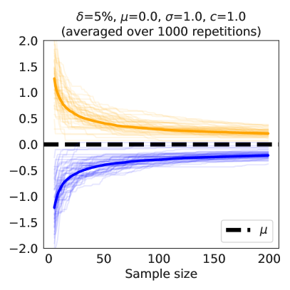
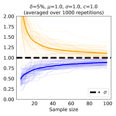
Figure 3: Examples of confidence upper and lower envelopes around unknown expectation $\mu=0$ for $\mathcal{N}\left(\mu,1\right)$ (left, cf. Table 2) and unknown standard deviation $\sigma=1$ for $\mathcal{N}\left(1,\sigma\right)$ (right, cf. Table 2), as a function of the number of observations $n$. The thick lines indicate the median curve over 1000 replicates.

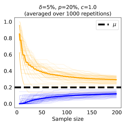
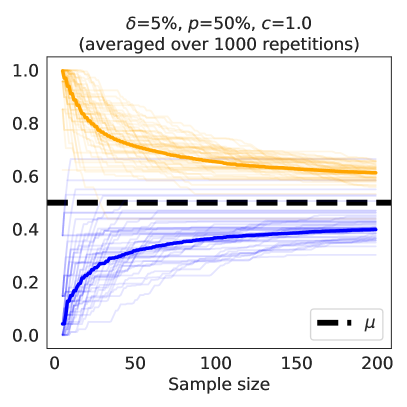
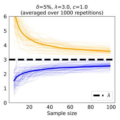
Figure 4: Examples of confidence upper and lower envelopes around expectation $\mu$ for discrete distributions. From top to bottom: $\text{Bernoulli}(p)$, $p\in\{0.2,0.5,0.8\}$ (cf. Table (2)) and $\text{Poisson}(3)$ (cf. Table 2) on several realizations (each dashed lines) as a function of the number of observations $n$. The thick lines indicate the median curve over 1000 replicates.

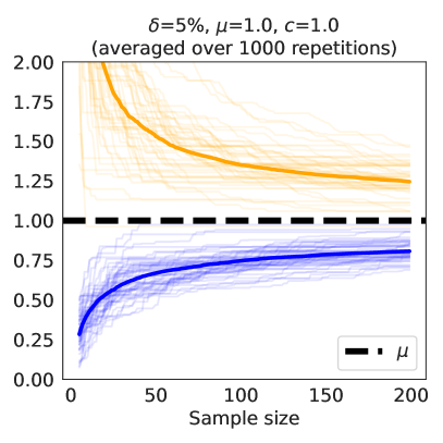
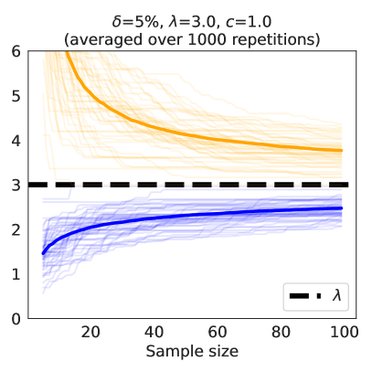
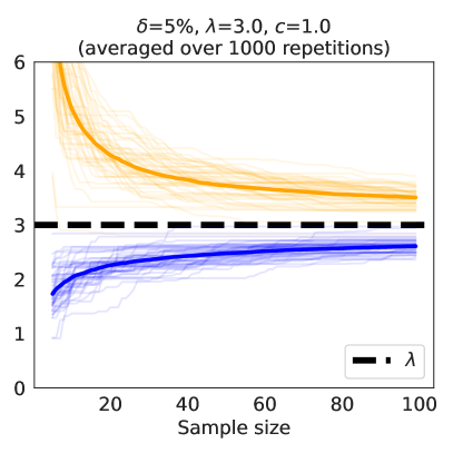
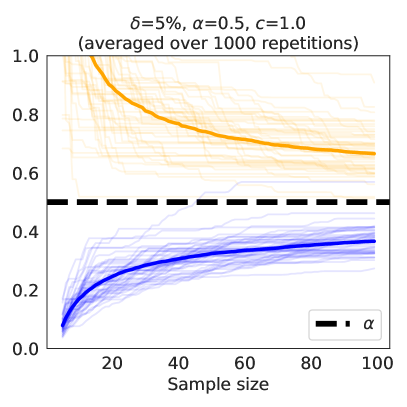
Figure 5: Examples of confidence upper and lower envelopes (from top to bottom) around scale parameter $\lambda$ for $\text{Exp}(1)$ (cf. Table (2)), fixed shape $\text{Gamma}(3,2)$ (cf. Table 2), fixed shape $\text{Weibull}(3,2)$ (cf. Table 2), and exponent $\alpha$ for $\text{Pareto}(\frac{1}{2})$ (cf. Table 2), on several realizations (each dashed lines) as a function of the number of observations $n$. The thick lines indicate the median curve over 1000 replicates.

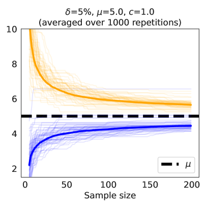
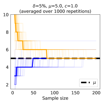
Figure 6: Examples of confidence upper and lower envelopes around expectation $\mu$ for (continuous prior) $\text{Gamma}\left(\frac{k}{2}\right)$ with unknown shape $\frac{k}{2}>0$ and (discrete prior) Chi-square $\chi^{2}(k)$, $k\in\mathbb{N}^{*}$ (cf. Table (2) and Remark 9) on several realizations (each dashed lines), as a function of the number of observations $n$. In particular for the Chi-square, confidence lower and upper bounds are ceiled and floored to integers. The thick lines indicate the median curve over 1000 replicates.

D.1 Gaussian with unknown mean and variance

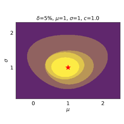
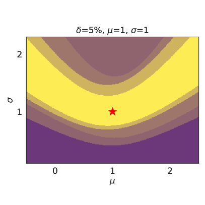
Figure 7: Example of time-uniform, joint confidence sets around $(\mu,\sigma)$ for $\mathcal{N}\left(1,1\right)$ (cf. Table 2 for $n\in\left\{10,25,50,100\right\}$ observations (smaller confidence sets correspond to larger sample sizes). The red star indicates the true parameters $(\mu,\sigma)=(1,1)$.

We consider the two-dimensional family $\left\{\mathcal{N}\left(\mu,\sigma^{2}\right),\left(\mu,\sigma\right)\in\mathbb{R}\times\mathbb{R}^{*}_{+}\right\}$. To the best of our knowledge, there does not exist time-uniform joint confidence sets for $\left(\mu,\sigma\right)$ prior to this work. In order to compare ourselves against some baseline, we derive a crude one based on Chi-square quantiles and a union bound.

Let $n\in\mathbb{N},\delta\in(0,1)$, $X_{1},\dots,X_{n}$ i.i.d samples from $\mathcal{N}(\mu_{0},\sigma_{0}^{2})$. The standardized sum of squares

$$Z_{t}(\mu_{0},\sigma_{0})=\sum\limits_{s=1}^{t}\left(\frac{X_{t}-\mu_{0}}{\sigma_{0}}\right)^{2}$$

follows a $\chi^{2}(t)$ distribution, therefore, denoting by $q_{\chi^{2}(t)}$ the corresponding quantile function, we have:

$$\mathbb{P}\left(q_{\chi^{2}(t)}\left(\frac{\delta}{2}\right)\leqslant Z_{t}(\mu_{0},\sigma_{0})\leqslant q_{\chi^{2}(t)}\left(1-\frac{\delta}{2}\right)\right)\geqslant 1-\delta\,.$$

By a union bound argument, the intersection of $n$ such events with confidence $\frac{\delta}{n}$, i.e

$$\Theta^{Z}_{t,n}(\delta)=\bigcap\limits_{s=1}^{t}\left\{(\mu,\sigma)\in\mathbb{R}\times\mathbb{R}_{+}^{*}\colon\ q_{\chi^{2}(s)}\left(\frac{\delta}{2n}\right)\leqslant Z_{s}(\mu,\sigma)\leqslant q_{\chi^{2}(s)}\left(1-\frac{\delta}{2n}\right)\right\}\,$$

describes a sequence of confidence sets at level $\delta$ that hold uniformly over $t\in\{1,\dots,n\}$.

We report our confidence sets (cf. Equation 2) and the above on Figure 7. The most striking drawback of $\Theta^{Z}_{t,n}(\delta)$ is that it is not convex nor even bounded; in particular, projecting onto the axes of $\mu$ and $\sigma$ only provides trivial confidence sets, $\mathbb{R}$ and $\mathbb{R}_{+}^{*}$ respectively, rendering this result vacuous. To better grasp this phenomenon, let us informally consider $\mu=\alpha+\mu_{0}$ and $\sigma=\alpha$ for some $\alpha>0$. We have:

$$Z_{n}(\mu,\sigma) =\sum\limits_{t=1}^{n}\left(\frac{X_{t}-\mu_{0}}{\alpha}-1\right)^{2}$$

$$=\underbrace{\frac{1}{\alpha^{2}}\sum\limits_{t=1}^{n}\left(X_{t}-\mu_{0}\right)^{2}}_{\approx\frac{\sigma_{0}^{2}}{\alpha^{2}}n}-\underbrace{\frac{2}{\alpha}\sum\limits_{t=1}^{n}\left(X_{t}-\mu_{0}\right)}_{\approx\frac{2}{\alpha}\sqrt{n}}+n\,.$$

Hence, for $\alpha\rightarrow+\infty$, $Z_{n}(\mu_{0}+\alpha,\alpha)\approx n$. On the other hand, Lemma 1 in Laurent and Massart (2000) shows that $q_{\chi^{2}(n)}\left(1-\delta/2n\right)=\mathcal{O}\left(n+\sqrt{n\log n}\right)$ and $q_{\chi^{2}(s)}\left(\delta/2n\right)=\mathcal{O}\left(n\right)$. Therefore, even with increasing the sample size $n$, there exists arbitrary large $\alpha$ such that $(\mu_{0}+\alpha,\alpha)$ may belong to $\Theta^{Z}_{t,n}(\delta)$.

By contrast, our Bregman confidence sets are convex and bounded, which we interpret as the result of exploiting the true geometry of the two-dimensional Gaussian family. In addition to the unboundedness, $\Theta^{Z}_{t,n}(\delta)$ is built using a crude union bound, which is not anytime (depends on the terminal time $n$) and rather loose.

D.2 Bernoulli

We consider the Bernoulli distribution $\text{Bernoulli}(\mu)$ for some unknown $\mu\in[0,1]$. Confidence bounds are displayed in Figure 8 for $\mu\in\{0.2,0.5,0.8\}$. We detail below a few alternative state-of-the-art bounds.

Chernoff-Laplace method for sub-Gaussian distributions

We recall that $B(\mu)$ being supported in $[0,1]$, it is $1/2$-sub-Gaussian (Hoeffding lemma, Hoeffding (1963)). The method of mixtures for exponential martingales (Peña et al., 2008) shows that $\mathbb{P}\left(\forall n\in\mathbb{N},\mu\in\Theta^{\text{Laplace}}_{n}(\delta)\right)\geqslant 1-\delta$, with

$$\Theta^{\text{Laplace}}_{n}(\delta)=\left[\widehat{\mu}_{n}-\sqrt{\left(1+\frac{1}{n}\right)\frac{\log\left(2\sqrt{1+n}/\delta\right)}{2n}},\widehat{\mu}_{n}+\sqrt{\left(1+\frac{1}{n}\right)\frac{\log\left(2\sqrt{1+n}/\delta\right)}{2n}}\right].$$

Note that a sharper sub-Gaussian control holds for $B(\mu)$, see Kearns and Saul (1998), Berend and Kontorovich (2013). However, the optimal sub-Gaussian parameter they suggest ($\frac{1/2-\mu}{\log(1/\mu-1)}$ instead of $1/2$) is a function of the unknown $\mu$.

Bentkus concentration with geometric time-peeling

Kuchibhotla and Zheng (2021, Theorem 4) show that $\mathbb{P}\left(\forall n\in\mathbb{N},\mu\in\Theta^{\text{Bentkus}}_{n}(\delta)\right)\geqslant 1-\delta$ with

$$\Theta^{\text{Bentkus}}_{n}(\delta)=\left[\widehat{\mu}_{n}-\frac{1}{n}q\left(\frac{\delta}{2h(k_{n})};c_{n},1/2,1\right),\widehat{\mu}_{n}+\frac{1}{n}q\left(\frac{\delta}{2h(k_{n})};c_{n},1/2,1\right)\right].$$

Here $q(\delta^{\prime};N,A,B)$ is the Bentkus bound, where $\delta^{\prime}$ is the confidence level, $N$ is the sample size, $B$ is the almost sure upper bound of the random variables and $A^{2}$ is the variance upper bound. The function $h(k)$ is defined as $h(k)=\zeta(1.1)(k+1)^{1.1}$, where $\zeta(\cdot)$ is the Riemann-zeta function. The integer $k_{n}$ and the real $c_{n}$ are defined as $k_{n}=\min\{k\in\mathbb{N}:\lceil\eta^{k}\rceil\leqslant n\leqslant\lfloor\eta^{k+1}\rfloor\}$ and $c_{n}=\lfloor\eta^{k_{n}+1}\rfloor$, with $\eta=1.1$. The referenced theorem is stated with an empirical overestimate of the standard deviation instead of the fixed bound $1/2$, which would lead to replace the $\delta/2$ present in the confidence set with $\delta/3$ by union bound; we found this step to be of negligible, and even slightly detrimental impact, in the case of Bernoulli distributions.

Hedged Capital martingale method

Waudby-Smith and Ramdas (2023, Theorem 3) present a nonnegative martingale construction from observations $X_{1},\dots,X_{n}$ bounded in $[0,1]$. Following the recommendations of the authors, we define the following quantities:

$$\mathcal{K}_{n}(m)=\max(\mathcal{K}_{n}^{+},\mathcal{K}_{n}^{-}(m)),$$

$$\mathcal{K}_{n}^{\pm}(m)=\prod_{k=1}^{n}\left(1\pm\lambda_{k}^{\pm}(m)\left(X_{k}-m\right)\right),$$

$$\lambda_{k}^{+}(m)=\min\left(\lvert\lambda_{k}\rvert,\frac{1/2}{m}\right),\lambda_{k}^{-}(m)=\min\left(\lvert\lambda_{k}\rvert,\frac{1/2}{1-m}\right),$$

$$\lambda_{k}=\sqrt{\frac{2\log(2/\delta)}{\widehat{\sigma}_{k-1}^{2}k\log(k+1)}},$$

$$\widehat{\sigma}_{k}^{2}=\frac{1/4+\sum_{i=1}^{k}\left(X_{i}-\widehat{\mu}_{i}\right)^{2}}{k+1},$$

$$\widehat{\mu}_{k}=\frac{1/2+\sum_{i=1}^{k}X_{i}}{k+1}.$$

Then, it holds that $\mathbb{P}\left(\forall n\in\mathbb{N},\mu\in\Theta^{\text{HC}}_{n}(\delta)\right)\geqslant 1-\delta$, where $\Theta^{\text{HC}}_{n}(\delta)=\left\{m\in[0,1]:\mathcal{K}_{n}(m)<1/\delta\right\}$.

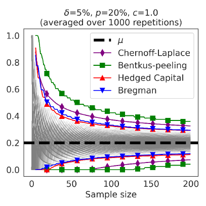
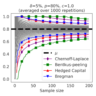
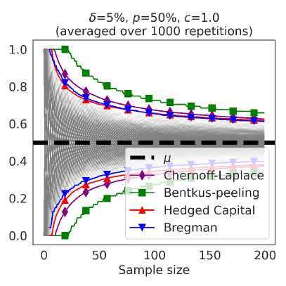
Figure 8: Confidence upper and lower envelopes built for $\text{Bernoulli}(\mu)$, $\mu\in\{0.2,0.5,0.8\}$, as a function of the number of observations $n$, averaged over $1000$ independent simulations. Grey lines are trajectories of empirical means $\widehat{\mu}_{n}$. Confidence bounds are clipped between $0$ and $1$.

D.3 Gaussian

We consider Gaussian distributions $\mathcal{N}(\mu,\sigma^{2})$ for some unknown $\mu\in\mathbb{R}$ and known variance $\sigma^{2}$. The confidence bounds are displayed in Figure 9 for $\mu=0$.

Chernoff-Laplace

Similarly to the Bernoulli case, $\mathcal{N}(\mu,\sigma^{2})$ is $\sigma$-sub-Gaussian, therefore
$\mathbb{P}\left(\forall n\in\mathbb{N},\mu\in\Theta^{\text{Laplace}}_{n}(\delta)\right)\geqslant 1-\delta$, with

$$\Theta^{\text{Laplace}}_{n}(\delta)=\left[\widehat{\mu}_{n}-\sigma\sqrt{\left(1+\frac{1}{n}\right)\frac{\log\left(2\sqrt{1+n}/\delta\right)}{n}},\widehat{\mu}_{n}+\sigma\sqrt{\left(1+\frac{1}{n}\right)\frac{\log\left(2\sqrt{1+n}/\delta\right)}{n}}\right].$$

Kaufmann-Koolen

Kaufmann and Koolen (2021) introduces a martingale construction for exponential families to derive time-uniform deviation inequalities under bandit sampling. However, application of their result is limited to Gaussian distribution with known variance and Gamma distribution with known shape, which is just a scaled version of exponential distribution. Restricting Corollary 10 of Kaufmann and Koolen (2021) to the case of a single arm yields $\mathbb{P}\left(\forall n\in\mathbb{N},\mu\in\Theta^{\text{KK}}_{n}(\delta)\right)\geqslant 1-\delta$, with

$$\Theta^{\text{KK}}_{n}(\delta)=\left\{\mathcal{B}_{\mathcal{L}}\left(\widehat{\mu}_{n},\mu\right)\leqslant\frac{2}{n}\log\left(4+\log(n)\right)+\frac{1}{n}C^{g}\left(\log 1/\delta\right)\right\},$$

$$g\colon\lambda\in(1/2,1]\mapsto 2\lambda\left(1-\log(4\lambda)\right)+\log\zeta(2\lambda)-\frac{1}{2}\log(1-\lambda),$$

$$C^{g}\colon x\in(0,+\infty)\mapsto\min_{\lambda\in(1/2,1]}\frac{g(\lambda)+x}{\lambda},$$

$$\mathcal{L}(\theta)=\frac{\theta^{2}}{2\sigma^{2}}\quad\text{(log-partition function of $\mathcal{N}(\cdot,\sigma^{2})$)}.$$

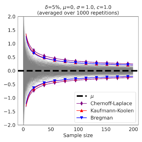
Figure 9: Confidence upper and lower envelopes built for Gaussian distributions $\mathcal{N}(0,1)$ as a function of the number of observations $n$, averaged over $1000$ independent simulations. Grey lines are trajectories of empirical means $\widehat{\mu}_{n}$.

D.4 Exponential

We now consider exponential distributions $\text{Exp}(1/\mu)$ for some unknown mean $\mu\in\mathbb{R}$. We report in Figure 10 the confidence bounds for the case when $\mu=1$.

Kaufmann-Koolen

Kaufmann and Koolen (2021, Corollary 12) show that $\mathbb{P}\left(\forall n\in\mathbb{N},\mu\in\Theta^{\text{KK}}_{n}(\delta)\right)\geqslant 1-\delta$, with the same definition as for the Gaussian case except

$$g\colon\lambda\in(1/2,1]\mapsto 2\lambda\left(1-\log(4\lambda)\right)+\log\zeta(2\lambda)-\log(1-\lambda),$$ (13)

$$\mathcal{L}(\theta)=\log(-1/\mu)\quad\text{(log-partition function of $\mathcal{E}(1/\mu)$)}.$$ (14)

Figure 10: Confidence upper and lower envelopes built for Exponential distributions $\text{Exp}(1)$ as a function of the number of observations $n$, averaged over $1000$ independent simulations. Grey lines are trajectories of empirical means $\widehat{\mu}_{n}$.

D.5 Chi-square

We consider $\text{Gamma}\left(\frac{k}{2},\frac{1}{2}\right)$ and $\chi^{2}\left(k\right)$ distributions for some unknown $k>0$ and $k\in\mathbb{N}^{*}$ respectively. They are in fact the same distributions, however we distinguish both as the restriction on the domain for $k$ (real or integer) bears two consequences:

• the mixture distribution in the martingale construction is either continuous or discrete, resulting in integrals or sums in the expression of the confidence sequence (Equation 2);

• confidence bounds are constrained to be integers in the discrete case, thus ceiling and flooring the lower and upper bounds respectively.

We find that the former is negligible as both the continuous and discrete mixtures yield the same bound within numerical precision. The latter however allows to drastically shrink the size of the confidence sequences, resulting in perfect identification the mean within $95\%$ confidence with less than $100$ observations in half the simulations (see Figure 11).

D.6 Key Observations

On the studied examples, confidence intervals based on time-uniform Bregman concentration are either comparable with state-of-the art methods for the corresponding setting or result in sharper bounds, especially for small sample sizes (lower bounds for Bernoulli compared to Hedged Capital, upper bound for Exponential compared to Kaufmann-Koolen). In particular, due to the formulation in terms of Bregman divergence, our intervals are naturally asymmetric when the underlying distribution is, and respect the support constraints (for instance Bernoulli Bregman bounds are in $[0,1]$ without the need for clipping). Moreover, we also provide bounds in novel settings for which, to the best of our knowledge, time-uniform confidence sets are lacking (Chi-square, Poisson, Weibull, Pareto, mean-variance for Gaussian).

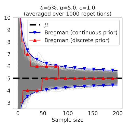
Figure 11: Confidence upper and lower envelopes built for $\text{Gamma}\left(\frac{5}{2},\frac{1}{2}\right)$ (blue) and $\chi^{2}\left(5\right)$ (red) distributions as a function of the number of observations $n$, over $1000$ independent simulations (colored lines are median of simulated bounds). Grey lines are trajectories of empirical means $\widehat{\mu}_{n}$.

D.7 Tuning of The Regularization Parameter $c$

In this section, we provide additional experiments regarding the local regularization parameter $c$. We study the sensitivity of the bounds to the values of $c$, reported in Figure 12. Then, we report in Figure 13 plots showing a tuning of parameter $c$ for each fixed $n=n_{0}$ illustrated for Bernoulli, Gaussian, exponential and Chi-square distributions. Specifically, $c$ is chosen to minimize the width of the confidence set at $n=n_{0}$, i.e., $c_{n_{0}}=\min_{c>0}\lvert\Theta_{n_{0},c}\left(\delta\right)\rvert$. Let us recall that such a tuning is only valid for a single value. Hence, while using $c=c_{n_{0}}$ for a fixed $n_{0}$ is allowed by the theory to produce time-uniform bounds for all $n$, using $c=c_{n}$, that is a different value for different $n$, is not supported by the theory as it would break the martingale property necessary for the mixture construction to hold, which is manifested by a contradiction with the law of iterated logarithm (see Section 3.1).

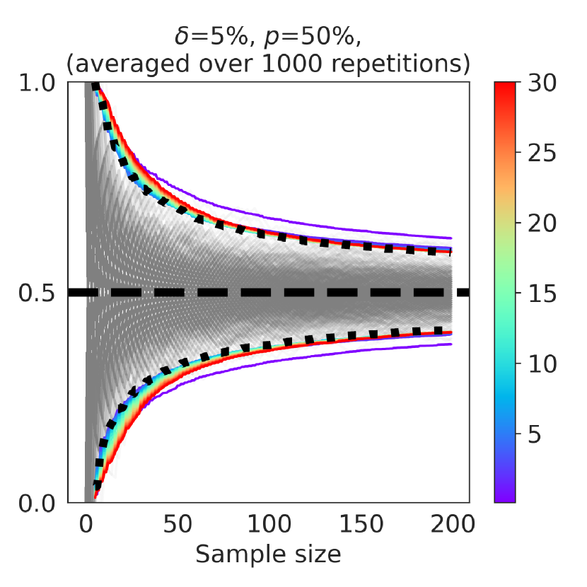
(a) Bernoulli

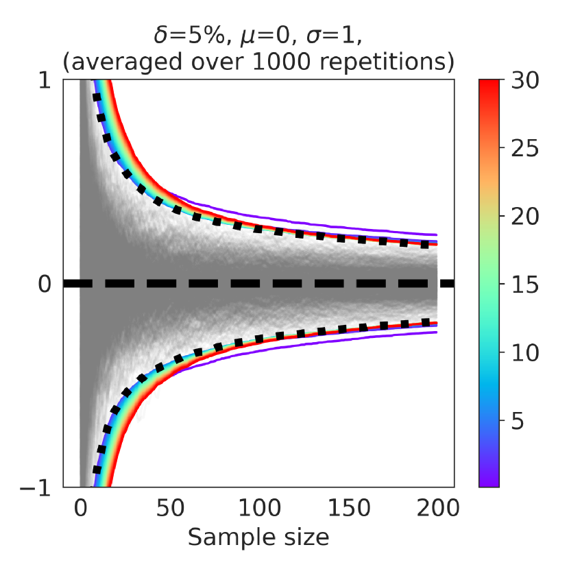
(b) Gaussian

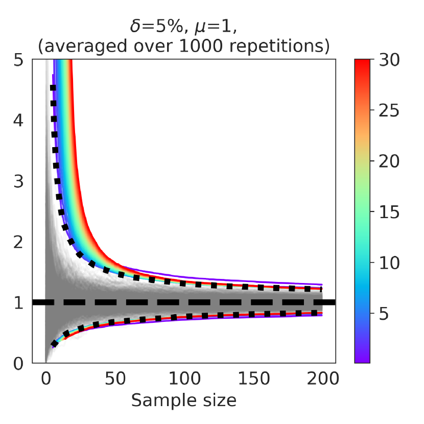
(c) Exponential

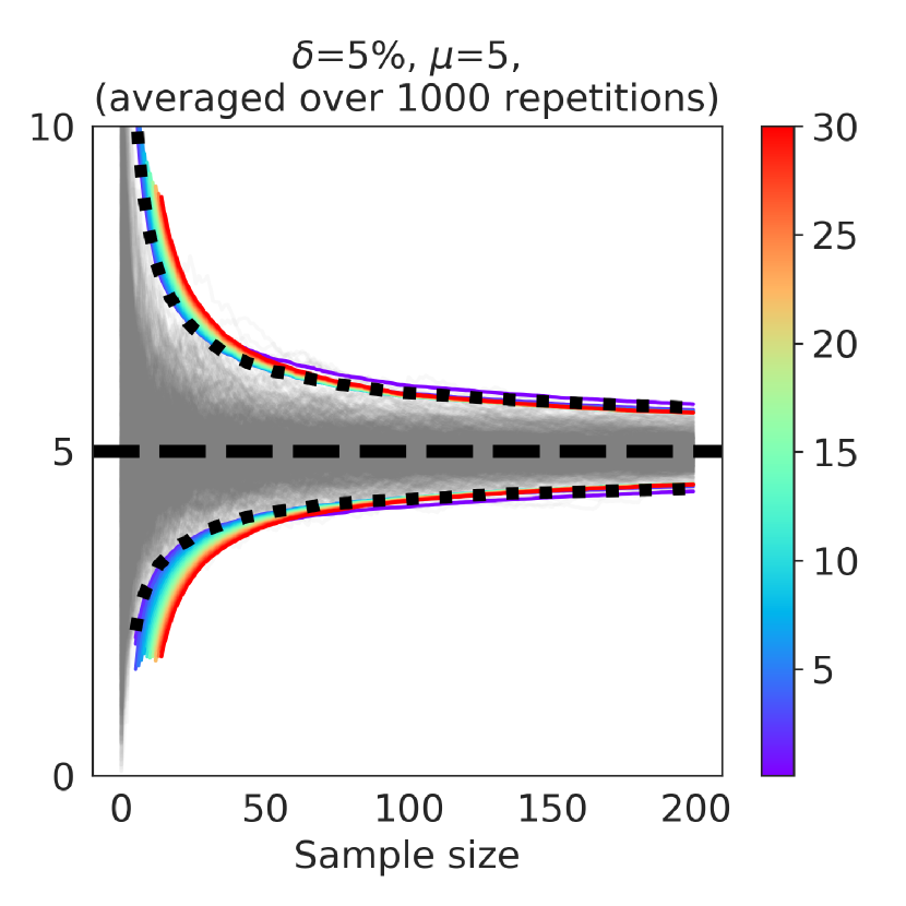
(d) Chi-square

Figure 12: Confidence envelopes for varying $c\in[0.1,30]$ for $\mathcal{B}(0.5)$ (top left), $\mathcal{N}(0,1)$ (top right), $\mathcal{E}(1)$ (bottom left) and $\chi^{2}(5)$ (bottom right). The dotted black line corresponds to the heuristics $c_{n}\approx 0.12n$.

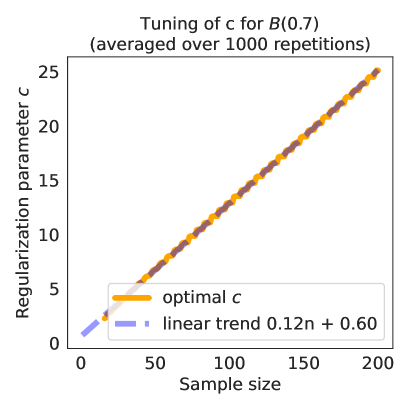
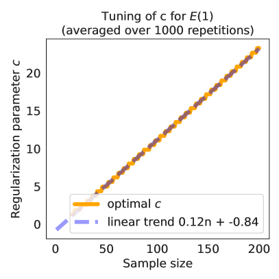
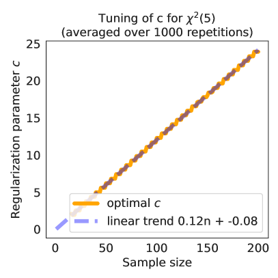
Figure 13: Optimal (smallest confidence interval diameter) local regularization parameter $c^{*}_{n}=\mathop{\mathrm{argmin}}_{c}\lvert\Theta_{n,c}\left(\delta\right)\rvert$ for $\delta=5\%$ on Bernoulli (top left), Gaussian (top right), exponential (bottom left) and Chi-square (bottom right). Note the apparent common linear trend $c^{*}_{n}\approx 0.12n$. Results are averaged over $1000$ independent simulations.

Appendix E Application: Generalized Likelihood Ratio Test in Exponential Families

In this section, we apply our result to revisit GLR tests in exponential families. The Generalized Likelihood Ratio (GLR) in the exponential family model $\mathcal{E}$ writes a follows

$$G^{\mathcal{E}}_{1:s:t} = \log\bigg{(}\frac{\sup_{\theta_{1},\theta_{2}}\prod_{t^{\prime}=1}^{s}p_{\theta_{1}}(X_{t^{\prime}})\prod_{t^{\prime}=s+1}^{t}p_{\theta_{2}}(X_{t^{\prime}})}{\sup_{\theta}\prod_{t^{\prime}=1}^{t}p_{\theta}(X_{t^{\prime}})}\bigg{)}$$

$$= \sup_{\theta_{1},\theta_{2}}\sum_{t^{\prime}=1}^{s}\log p_{\theta_{1}}(X_{t^{\prime}})+\sum_{t^{\prime}=s+1}^{t}\log p_{\theta_{2}}(X_{t^{\prime}})-\sup_{\theta}\sum_{t^{\prime}=1}^{t}\log p_{\theta}(X_{t^{\prime}})$$

$$= s\mathcal{L}^{\star}(F_{1:s})+(t-s)\mathcal{L}^{\star}(F_{s+1:t})-t\mathcal{L}^{\star}(F_{1:t})$$

$$= s(\mathcal{L}^{\star}(F_{1:s})-\mathcal{L}^{\star}(F_{1:t}))+(t-s)(\mathcal{L}^{\star}(F_{s+1:t})-\mathcal{L}^{\star}(F_{1:t}))\,,$$

where $F_{s+1:t}=\frac{1}{t-s}\sum_{t^{\prime}=s+1}^{t}F(X_{t^{\prime}})$, and it makes sense to introduce $\theta_{s+1:t}$ such that $\nabla\mathcal{L}(\theta_{s+1:t})=F_{s+1:t}$. The GLR test is then defined, for a threshold $\alpha$ as

$$\tau(\alpha;\mathcal{E}) = \min\{t\in\mathbb{N}:\max_{s\in[0,t)}G^{\mathcal{E}}_{1:s:t}\geqslant\alpha\}$$

An alternative formulation of the GLR shows that

$$G^{\mathcal{E}}_{1:s:t} =\inf_{\theta}\sup_{\theta_{1},\theta_{2}}\log\bigg{(}\frac{\prod_{t^{\prime}=1}^{s}p_{\theta_{1}}(X_{t^{\prime}})\prod_{t^{\prime}=s+1}^{t}p_{\theta_{2}}(X_{t^{\prime}})}{\prod_{t^{\prime}=1}^{t}p_{\theta}(X_{t^{\prime}})}\bigg{)}$$

$$=\inf_{\theta}\sup_{\theta_{1},\theta_{2}}s\Big{(}\langle\theta_{1},F_{1:s}\rangle-\mathcal{L}(\theta_{1})-\langle\theta,F_{1:t}\rangle+\mathcal{L}(\theta)\Big{)}$$

$$\quad+(t-s)\Big{(}\langle\theta_{2},F_{s+1:t}\rangle-\mathcal{L}(\theta_{2})-\langle\theta,F_{1:t}\rangle+\mathcal{L}(\theta)\Big{)}\,.$$

The first supremum is obtained for $\theta_{1}=[\nabla\mathcal{L}]^{-1}(F_{1:s})$, with value equal to $\mathcal{B}_{\mathcal{L}}(\theta,\theta_{1})+\langle\theta-\theta_{1},\nabla\mathcal{L}(\theta_{1})\rangle+\langle\theta_{1},F_{1:s}\rangle+\langle\theta_{1},F_{1_{t}}\rangle$, that is $\mathcal{B}_{\mathcal{L}}(\theta,\theta_{1:s})+\langle\theta,F_{1:s}-F_{1:t}\rangle$. Likewise, the the second supremum is obtained for $\theta_{2}=[\nabla\mathcal{L}]^{-1}(F_{s+1:t})$, with value equal to $\mathcal{B}_{\mathcal{L}}(\theta,\theta_{s+1:t})+\langle\theta,F_{s+1:t}-F_{1:t}\rangle$. Combining these two results, and remarking that $s(F_{1:s}-F_{1:t})+(t-s)(F_{s+1:t}-F_{1:t})=0$, we obtain that

$$G^{\mathcal{E}}_{1:s:t} = \inf_{\theta}s\mathcal{B}_{\mathcal{L}}(\theta,\theta_{1:s})+(t-s)\mathcal{B}_{\mathcal{L}}(\theta,\theta_{s+1:t})$$ (15)

We further note that a solution to this optimization problem is obtained for $\theta$ such that $s(\nabla L(\theta)-\nabla L(\theta_{1:s}))+(t-s)(\nabla L(\theta)-\nabla L(\theta_{s+1:t}))=0$. Reorganizing the terms, this entails that $\nabla L(\theta)=\frac{1}{t}(sF_{1:s}+(t-s)F_{s+1:t})=F_{1:t}$, and thus (without surprise) $\theta=\theta_{1:t}$.

Written in the form (15), the GLR satisfies for any $\theta^{\prime}$,

$$G^{\mathcal{E}}_{1:s:t} \leqslant s\mathcal{B}_{\mathcal{L}}(\theta^{\prime},\theta_{1:s})+(t-s)\mathcal{B}_{\mathcal{L}}(\theta^{\prime},\theta_{s+1:t})\,.$$

In particular, the false alarm rate of the GLR test, when all observations are generated from parameter $\theta$, can be bounded using

$$\mathbb{P}_{\theta}(\tau(\alpha;\mathcal{E})<\infty) = \mathbb{P}_{\theta}\big{(}\exists(t,s)\in\mathbb{N}^{2},s<t:G^{\mathcal{E}}_{1:s:t}\geqslant\alpha\big{)}$$

$$\leqslant \mathbb{P}_{\theta}\Big{(}\exists(t,s)\in\mathbb{N}^{2},s<t:s\mathcal{B}_{\mathcal{L}}(\theta,\theta_{1:s})+(t-s)\mathcal{B}_{\mathcal{L}}(\theta,\theta_{s+1:t})\geqslant\alpha\Big{)}\,.$$

At this point, provided that for appropriate terms $\alpha_{1},\alpha_{2}$,

$$\mathbb{P}_{\theta}\Big{(}\exists s\in\mathbb{N}:s\mathcal{B}_{\mathcal{L}}(\theta,\theta_{1:s})\geqslant\alpha_{2}\Big{)}\leqslant\frac{\delta}{2}\,,$$

$$\mathbb{P}_{\theta}\Big{(}\exists(t,s)\in\mathbb{N}^{2},s<t:(t-s)\mathcal{B}_{\mathcal{L}}(\theta,\theta_{s+1:t})\geqslant\alpha_{1}\Big{)}\leqslant\frac{\delta}{2}\,.$$

we deduce by a simple union bound argument, and for $\alpha=\alpha_{1}+\alpha_{2}$ that $\mathbb{P}_{\theta}(\tau(\alpha:\mathcal{E})<\infty)\leqslant\delta$.

A regularized GLR test

Our concentration result shows that such a controlled can be obtained for a penalized version of the maximum likelihood parameter estimates $\theta_{1:s},\theta_{s+1,t},\theta_{1,t}$. Namely, let us consider the set

$$\Theta_{s,c}(\delta) = \bigg{\{}\theta\in\Theta:\exists s\in\mathbb{N}:s\mathcal{B}_{\mathcal{L}}(\theta,\theta_{1:s,c}(\theta))\geqslant\alpha_{1}\bigg{\}}\,,$$

$$\Theta_{s+1:t,c}(\delta) = \bigg{\{}\theta\in\Theta:\exists(t,s)\in\mathbb{N}^{2},s<t:(t-s)\mathcal{B}_{\mathcal{L}}(\theta,\theta_{s+1:t,c}(\theta))\geqslant\alpha_{2}\bigg{\}}\,.$$

Provided that $\alpha_{1}$ and $\alpha_{2}$ are defined to ensure that these are high-probability confidence sets for the parameter $\theta_{0}$, then they should have non-empty intersections under $\mathbb{P}_{\theta}$. This motivates the following definition of the regularized GLR-test:

$$\tau^{\delta}_{c}(\mathcal{E}) = \min\left\{t\in\mathbb{N}:\exists s\!<\!t,\Theta_{s,c}(\delta/2)\cap\Theta_{s+1:t,c}(\delta/2)=\emptyset\right\}\,.$$

The appropriate quantity for $\alpha_{1}$ is immediately obtained by Theorem 3 as $\frac{s}{s+c}(\log(1/\delta)+\gamma_{1:s,c}(\theta))$. Now for $\alpha_{2}$, we need to study doubly-time uniform concentration inequalities over both $s$ and $t$.

E.1 Doubly-time uniform concentration inequalities for exponential families

See 5

Proof of Theorem 5:

We consider that all the $(X_{t^{\prime}})_{t^{\prime}\in\mathbb{N}}$ come from a distribution with same parameter $\theta$. Let $t\in\mathbb{N}$ and $s\in\{0,\dots,t-1\}$. We introduce the scan-mean $\mu_{s+1:t}=\frac{1}{t-s}\sum_{t^{\prime}=s+1}^{t}F(X_{t^{\prime}})$ and its mean $\mu=\nabla\mathcal{L}(\theta)$. We define as in the proof of Theorem 3, for each $\lambda$ the martingale

$$M_{s+1:t}^{\lambda} = \exp\bigg{(}\langle\lambda,(t-s)(\mu_{s+1:t}-\mu)\rangle-(t-s)\mathcal{B}_{\mathcal{L},\theta}(\lambda)\bigg{)}\,.$$

Then, applying the method of mixture and replacing each term with its scan version from $s+1$ to $t$, we introduce the quantity

$$M_{s+1,t} = \exp\big{(}(t\!-\!s\!+\!c)\mathcal{B}_{\mathcal{L},\theta}^{\star}(x)\big{)}\frac{G(\theta,c)}{G(\theta_{s+1:t,c}(\theta_{0}),t-s+c)}$$

where $x=\frac{t\!-\!s}{t\!-\!s\!+\!c}(\mu_{s+1:t}-\nabla\mathcal{L}(\theta))$ and $\theta_{s+1:t,c}(\theta)$ is the regularized estimate from the scan samples

$$\theta_{s+1:t,c}(\theta)=(\nabla\mathcal{L})^{-1}\bigg{(}\frac{\sum_{t^{\prime}=s+1}^{t}F(X_{t^{\prime}})+c\nabla\mathcal{L}(\theta)}{t\!-\!s\!+\!c}\bigg{)}\,.$$

Remarking that $\mathbb{E}[M_{t,t}]\leqslant\mathbb{E}[M_{t+1,t}]=1$ and that $(M_{s+1,t})_{s}$ is a nonnegative supermartingale, we can now control its doubly-time uniform deviations following the proof of Maillard (2019b)[Th.3.2, p.58]. More precisely, for any non-decreasing function $g$, it can be shown that

$$\mathbb{P}_{\theta}\big{[}\exists t,\exists s<t:M_{s+1,t}\geqslant\frac{g(t)}{\delta}\big{]}\leqslant\delta\mathbb{E}_{\theta}\Big{[}\max_{t}\max_{s<t}\frac{M_{s+1:t}}{g(t)}\Big{]}\leqslant\delta\sum_{t=1}^{\infty}\frac{1}{g(t)}\,.$$

Rewriting the terms thanks to the duality formulas, yields

$$\mathbb{P}_{\theta}\bigg{[}\exists t,\exists s<t:(t\!-\!s\!-\!c)\mathcal{B}_{\mathcal{L}}(\theta,\theta_{s+1:t,c}(\theta))\geqslant\log\Big{(}\frac{g(t)}{\delta}\Big{)}+\gamma_{s+1:t,c}(\theta)\bigg{]}\leqslant\delta\sum_{t=1}^{\infty}\frac{1}{g(t)}\,.$$

This suggests to set $\alpha_{2}=\frac{t\!-\!s}{t\!-\!s\!-\!c}\left(\log\left(\frac{g(t)}{\delta}\right)+\gamma_{s+1:t,c}(\theta)\right)$ in the definition of the regularized GLR test. Putting all terms together, this leads to the definition of the following regularized GLR test, for a given false-detection error probability $\delta\in[0,1]$ and regularization parameter $c$,

$$\Theta_{s,c}(\delta)=\left\{\theta\in\Theta:(s\!+\!c)\mathcal{B}_{\mathcal{L}}(\theta,\theta_{1:s,c}(\theta))\leqslant\log(1/\delta)+\gamma_{1:s,c}(\theta)\right\}\,,$$

$$\Theta_{s+1:t,c}(\delta)=\left\{\theta\in\Theta:(t\!-\!s+\!c)\mathcal{B}_{\mathcal{L}}(\theta,\theta_{s+1:t,c}(\theta))\leqslant\log(g(t)/\delta)+\gamma_{s+1:t,c}(\theta)\right\}\,,$$

$$\tau^{\delta}_{c}(\mathcal{E})=\min\left\{t\in\mathbb{N}:\exists s\!<\!t,\Theta_{s,c}(\delta/2)\cap\Theta_{s+1:t,c}(\delta/2)=\emptyset\right\}\,.$$

The factor $g(t)$ that inflates the width of the confidence set can be tuned to satisfy $\sum_{t=1}^{+\infty}1/g(t)\leqslant 1$, thus controlling the above deviation probability by at most $\delta$ (ideally, $\sum_{t=1}^{+\infty}1/g(t)$ should be close to $1$ to avoid overinflating the confidence width). A natural choice for this is $g(t)=\kappa(1\!+\!t)\log^{2}(1\!+\!t)$ where $\kappa=2.10974\geqslant\sum_{t=1}^{\infty}\frac{1}{(1\!+\!t)\log^{2}(1\!+\!t)}$ (for completeness, we derive in the next section an elementary way to computing suitable values for $\kappa$). By construction, this test is guaranteed to have a false-detection probability controlled by $\delta$ (that is, $\mathbb{P}_{\theta}(\tau^{\delta}_{c}(\mathcal{E})<\infty)\leqslant\delta$).

Doubly time-uniform control of supermartingale sequences

For completeness, we reproduce below the derivation from Maillard (2019b)[Th.3.2, p.58], applied to our setup. First, let us note that

$$\mathbb{P}\bigg{(}\exists t\!\in\!\mathbb{N}_{\star},\exists s\!\in\![0,t-1],\,\,M_{s+1:t}\geqslant\frac{g(t)}{\delta}\bigg{)} = \mathbb{P}\bigg{(}\max_{t\in\mathbb{N}_{\star}}\max_{s\in[0,t-1]}\frac{M_{s+1:t}}{g(t)}\geqslant\frac{1}{\delta}\bigg{)}$$

$$\leqslant \delta\mathbb{E}\bigg{[}\max_{t\in\mathbb{N}_{\star}}\max_{s\in[0,t-1]}\frac{M_{s+1:t}}{g(t)}\bigg{]}\,.$$

Let us also denote $\tau$ the random stopping time corresponding to the first occurrence $t$ of the event $\max_{s\in[0,t-1]}\frac{M_{s+1:t}}{g(t)}\geqslant\frac{1}{\delta}$. It is convenient to introduce the quantity $\overline{M}_{t}=\frac{\sum_{s\in\{0,\dots,t-1\}}M_{s+1,t}}{g(t)}$ for each $t\in\mathbb{N}_{\star}$. Since each $M_{s+1,t}$ and $g(t)$ is nonnegative, we first get that for every random stopping time $\tau\in\mathbb{N}_{\star}$, the following inequality holds:

$$\mathbb{E}\bigg{[}\frac{\max_{s<\tau}M_{s+1,\tau}}{g(\tau)}\bigg{]} \leqslant \mathbb{E}\bigg{[}\overline{M}_{\tau}\bigg{]}=\mathbb{E}\bigg{[}\overline{M}_{1}+\sum_{t=1}^{\infty}(\overline{M}_{t+1}-\overline{M}_{t})\mathbb{I}\{\tau>t\}\bigg{]}\,.$$

Furthermore, we note that, conveniently

$$\overline{M}_{t+1}-\overline{M}_{t} = \frac{M_{t+1,t+1}}{g(t+1)}+\sum_{s=0}^{t-1}\bigg{(}\frac{M_{s+1,t+1}}{g(t+1)}-\frac{M_{s+1,t}}{g(t)}\bigg{)}\,.$$

Next, by assumption, we note that $\displaystyle{\mathbb{E}[M_{s+1,t+1}|\mathcal{F}_{t}]\leqslant M_{s+1,t}}$. Thus, since $\mathbb{I}\{\tau>t\}\in\mathcal{F}_{t}$, we deduce that

$$\mathbb{E}\bigg{[}\frac{\max_{s<\tau}M_{s+1,\tau}}{g(\tau)}\bigg{]}$$

$$\quad\leqslant\mathbb{E}\big{[}\overline{M}_{1}\big{]}+\sum_{t=1}^{\infty}\frac{\mathbb{E}[M_{t+1,t+1}]}{g(t+1)}+\sum_{t=1}^{\infty}\sum_{s<t}\mathbb{E}\bigg{[}\bigg{(}\frac{1}{g(t+1)}-\frac{1}{g(t)}\bigg{)}M_{s+1,t}\mathbb{I}\{\tau>t\}\bigg{]}$$

$$\quad=\mathbb{E}\big{[}\overline{M}_{1}\big{]}+\sum_{t=1}^{\infty}\frac{\mathbb{E}[M_{t+1,t+1}]}{g(t+1)}+\sum_{t=1}^{\infty}\sum_{s<t}\bigg{(}\frac{1}{g(t+1)}-\frac{1}{g(t)}\bigg{)}\underbrace{\mathbb{E}\bigg{[}M_{s+1,t}\mathbb{I}\{\tau>t\}\bigg{]}}_{\geqslant 0}\,.$$

Hence, the assumption that $g$ is non-decreasing ensures that the last sum is upper bounded by $0$. Since on the other hand $\mathbb{E}[M_{t+1,t+1}]\leqslant 1$ holds for all $t$ (and thus $\mathbb{E}\big{[}\overline{M}_{1}\big{]}\leqslant 1/g(1)$), we deduce that the following inequality holds:

$$\mathbb{E}\bigg{[}\frac{\max_{s<\tau}M_{s+1,\tau}}{g(\tau)}\bigg{]} \leqslant \frac{1}{g(1)}+\sum_{t=1}^{\infty}\frac{1}{g(t+1)}=\sum_{t=1}^{\infty}\frac{1}{g(t)}\leqslant 1\,.$$

$\hfill\square$

E.2 Computing the inflating factor $g(t)$

The right-hand side of the doubly time-uniform confidence set of Theorem 5 involves a $\log g(t)/\delta$ term instead of $\log 1/\delta$ as in Theorem 3, which is a by-product of the union-like argument used in the proof. Ideally, $g(t)$ should grow as slow as possible with $t$ to avoid unnecessary looseness in the confidence bound. That is however limited by the constraint $\sum_{t=1}^{\infty}1/g(t)\leqslant 1$, which prohibits the use of a linearly growing $g(t)$ (since $\sum_{t=1}^{\infty}1/t$ diverges). The choice $g(t)=\kappa(1\!+\!t)\log^{1\!+\!\eta}(1\!+\!t)$ for some $\eta>0$ and $\kappa>0$ guarantees that the series of inverses converges, although its limit is not available in closed-form. However, it is sufficient to set $\kappa$ to an upper bound on $\sum_{t=1}^{\infty}\frac{1}{(1\!+\!t)\log^{1\!+\!\eta}(1\!+\!t)}$. The following elementary lemma explains how to compute a tight value for $\kappa$.

Lemma 12

Let $f\colon t\in\mathbb{N}\mapsto(1\!+\!t)\log^{1\!+\!\eta}(1\!+\!t)$ and define $S_{p}=\sum_{t=1}^{p}1/f(t)$ for $p\in\mathbb{N}\cup\{+\infty\}$. Then $S_{\infty}\leqslant S_{p}+\frac{1}{\eta\log(1+p)^{\eta}}$.

Proof of Lemma 12:

The function $f$ is nondecreasing and positive, therefore for $t\in\mathbb{N}$ and $x\in[t,t+1)$, it holds that $1/f(t+1)\leqslant 1/f(x)$. Integrating both terms as functions of $x$ over the interval $[t,t+1)$ yields $1/f(t+1)\leqslant\int_{t}^{t+1}1/f(x)dx$. Summing starting at $t=p$, we further get the following sum-integral comparison:

$$S_{\infty}-S_{p}\leqslant\int_{p}^{\infty}\frac{dx}{f(x)}\,.$$

Finally, note that $\frac{d}{dx}\frac{1}{\eta\log^{\eta}(1+x)}=-\frac{1}{f(x)}$, and thus $\int_{p}^{\infty}\frac{dx}{f(x)}=\frac{1}{\eta\log(1+p)^{\eta}}$. $\hfill\square$

This lemma shows that $\kappa=S_{p}+1/\log(1\!+\!p)$ for some $p\geqslant 1$ ($\eta=1$) is a valid choice for the definition of the inflating factor $g(t)$, and is straightforward to compute numerically. For $p=100$, we obtain $\kappa\lesssim 2.10974$ and increasing $p$ only changes further digits.

E.3 Experiments on change point detection for Gaussian with unknown variance

We illustrate the change point GLR test above in a numerical experiment as follows. We consider the one-dimensional exponential family of centered Gaussian distributions with unknown variance $\mathcal{E}=\left\{\mathcal{N}(0,\sigma^{2}),\sigma>0\right\}$. A sequence of independent random variables $(X_{t})_{t\in\mathbb{N}}$ is drawn from $X_{t}\sim\mathcal{N}(0,\sigma_{0}^{2})$ if $t\leqslant t^{*}$ and from $X_{t}\sim\mathcal{N}(0,\sigma_{1}^{2})$ if $t>t^{*}$, where $t^{*}=50$ and $\sigma_{0}=1$ and $\sigma_{1}\in[1,2,3,4]$. Of note, this setting corresponds to an open question in Maillard (2019a), which studies GLR tests in sub-Gaussian families, which are adapted to the detection of changing means but not variances. Detection times are reported as $\min(\tau^{\delta}_{c}(\mathcal{E}),T)$ with $T=100$, and $\tau^{\delta}_{c}(\mathcal{E})>T$ is interpreted as no change being detected. For the doubly time-uniform confidence set in the definition of the regularized GLR test, we use the factor $g(t)=\kappa(1\!+\!t)\log^{2}(1\!+\!t)$ with $\kappa=2.10974$.

A practical motivation for this setting is, for instance, the design of maintenance models for equipment: with time, a component of a physical system (mechanical component, measuring instrument…) starts to wear off and while it is still functioning (same output on average), it is more imprecise or less stable (higher output variance); the goal of the maintenance agent is to detect as early as possible such changes of regime in order to replace the failing component before it breaks completely.

In Figure 14, we report the histograms of detection times across $1000$ independent simulations for increasingly abrupt changes of variance ($\sigma_{1}\in\{1,2,3,4\}$). As expected, the distribution of detection times shifts closer to the actual change point $t^{*}$ when $\sigma_{1}$ increases, i.e., more obvious changes are detected earlier. This is confirmed in Figure 15, where we report the median and interquartile range of detection times for $\sigma_{1}\in[1,4]$.

We empirically validate in Figure 14(a) the control of the false positive probability by at most $\delta=5\%$. However, the actual false positive rate appears much lower ($0.2\%$), which is a consequence of the looseness of the union bound involving the factor $g(t)$ in the doubly time-uniform confidence set. Following Maillard (2019a), a sharper approach would involve a direct concentration result on the pair $\left(\theta_{s,c},\theta_{s+1:t,c}\right)$ (i.e., in the terminology of Maillard (2019a), a joint bound, as opposed to the current disjoint one). This is a nontrivial result which we leave for future work. Finally, note that the high false negative rate of Figure 14(b) (27.6%) is an artifact of thresholding the detection time at $T=100$; increasing $T$ would enable later detections, thus reducing the number of observed false negatives, at the cost of increasing the average detection delay (as well as the computational burden of the experiment).

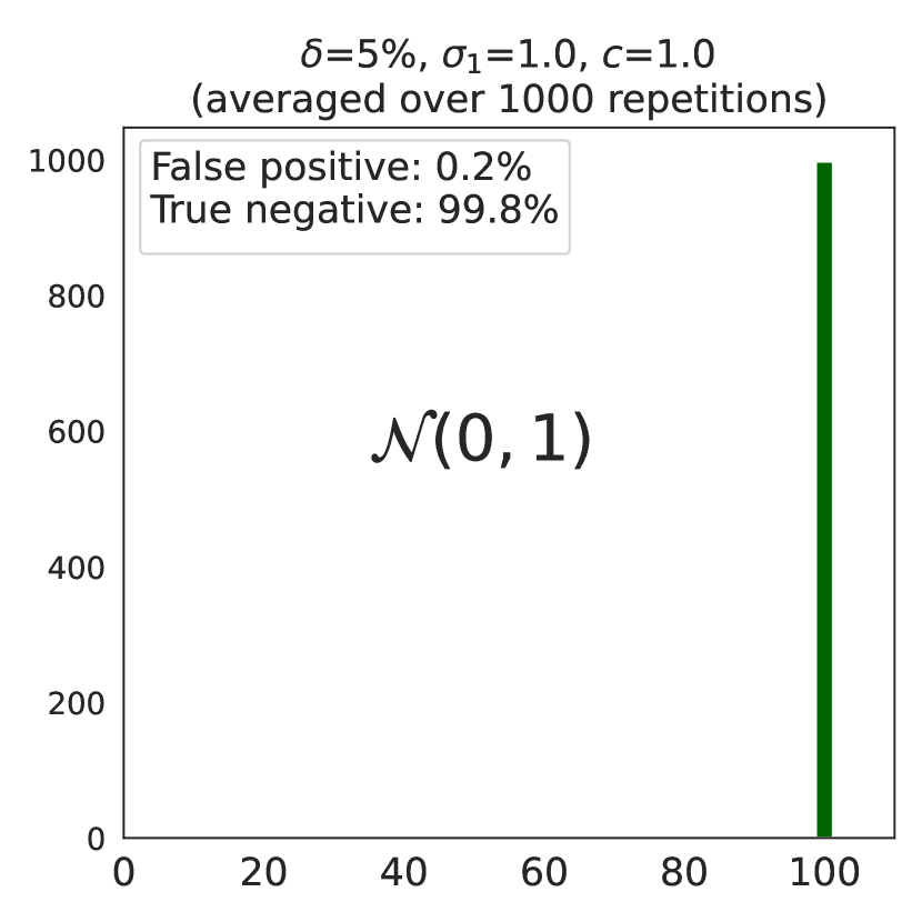
(a) $\sigma_{0}=\sigma_{1}=1$ (no change)

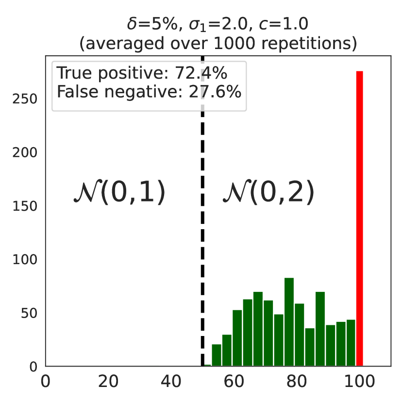
(b) $\sigma_{0}=1,\sigma_{1}=2$

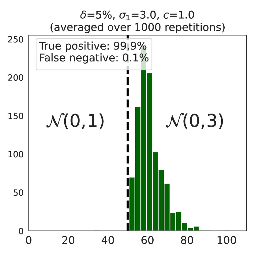
(c) $\sigma_{0}=\sigma_{1}=3$

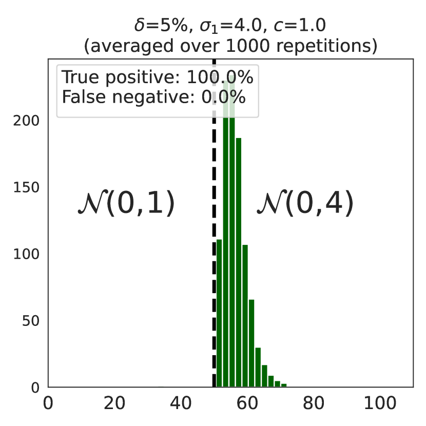
(d) $\sigma_{0}=1,\sigma_{1}=4$

Figure 14: Histograms of detection times $\tau^{\delta}_{c}(\mathcal{E})$ in the Gaussian setting described in Appendix E.3. Green: correct detection (negative in (a), positive in (b), (c) and (d)). Red: incorrect detection (positive in (a), negative in (b), (c) and (d)). Black dashed line: change point $t^{*}$.

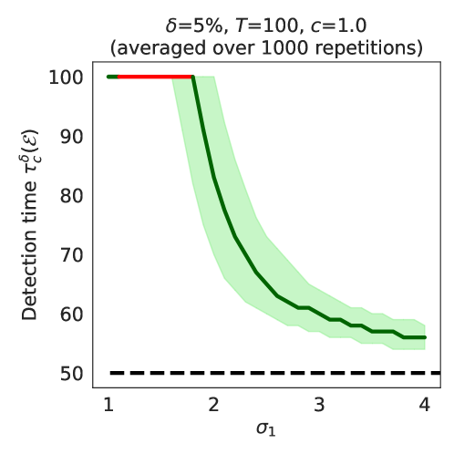
Figure 15: Detection time $\tau^{\delta}_{c}(\mathcal{E})$ in the Gaussian setting described in Appendix E.3. Solid line: median detection time. Shaded area: interquartile range of detection times (25th and 75th percentiles). Black dashed line: change point $t^{*}$.

Appendix F Application: Linear Contextual Bandits

In this section, we apply Theorem 7 to build confidence sets in the well-known linear bandit setting. We consider the setting of linear contextual bandits (Auer et al., 2002; Abbasi-Yadkori et al., 2011), but with possibly arm-dependent noise variance (heteroscedastic noise). An algorithm for this problem chooses, at each round $t\in\mathbb{N}$, an action or arm $A_{t}\!\in\!\mathcal{A}$, and subsequently observes a reward $X_{t}=\theta^{\top}\varphi(A_{t})+\varepsilon_{t}$, where $\varphi\!:\mathcal{A}\to\mathbb{R}^{d}$ is a (fixed) map from actions to their context vectors, $\theta\in\mathbb{R}^{d}$ is a vector of weights unknown to the algorithm and given the action $A_{t}$, $\varepsilon_{t}\sim\mathcal{N}(0,\sigma_{A_{t}}^{2}I)$ is a Gaussian noise with known variance $\sigma^{2}_{A_{t}}$. The goal is to select actions to maximize the expected cumulative reward $\sum_{t}\theta^{\top}\varphi(A_{t})$. Any rational agent would choose the action $A_{t}$ causally depending upon the history of arms and reward sequences available before the start of round $t$. Naturally, for each $n\!\in\!\mathbb{N}$, it boils down to controlling the deviation between the unknown parameter $\theta$ and a suitable estimate $\theta_{n}$ built from $n$ observations $(A_{t},X_{t})_{t\leqslant n}$.

Under this observation model, the feature function and the log-partition function are given by $F_{t}(x)=\frac{x}{\sigma_{A_{t}}^{2}}\varphi(A_{t})$ and $\mathcal{L}_{t}(\theta)=\frac{1}{2\sigma_{A_{t}}^{2}}\|\theta\|^{2}_{\varphi(A_{t})\varphi(A_{t})^{\top}}$. Let us define the matrix

$$V_{n}=\sum_{t=1}^{n}\frac{1}{\sigma_{A_{t}}^{2}}\varphi(A_{t})\varphi(A_{t})^{\top}\,,$$

and introduce the Legendre function $\mathcal{L}_{0}(\theta)=\frac{1}{2}\|\theta\|^{2}_{V_{0}}$, where $V_{0}$ is some fixed positive definite matrix. Then, the parameter estimate and the Bregman information gain take the form

$$\theta_{n,\mathcal{L}_{0}}=\left(V_{n}+V_{0}\right)^{-1}\sum_{t=1}^{n}\frac{X_{t}}{\sigma_{A_{t}}^{2}}\varphi(A_{t})~{},\quad\gamma_{n,\mathcal{L}_{0}}=\log\frac{\det(V_{0}+V_{n})^{1/2}}{\det(V_{0})^{1/2}}~{}.$$

Now, defining $\mathcal{H}_{t-1}:=\{A_{1},X_{1},\ldots,A_{t-1},X_{t-1},A_{t}\}$ to be the set of all information available before observing $X_{t}$, one can see that the confidence set $\Theta_{n,\mathcal{L}_{0}}(\delta)$ given by Theorem 7 is the set of all $\theta\in\Theta$ satisfying

$$\|\theta-\theta_{n,\mathcal{L}_{0}}\|^{2}_{V_{n}+V_{0}}\leqslant\|\theta\|^{2}_{V_{0}}+2\log\frac{\det(V_{0}+V_{n})^{1/2}}{\delta\det(V_{0})^{1/2}}.$$

Comparison with Existing Results

Under the assumption that the noise $\varepsilon_{t}$ is $\sigma_{A_{t}}$-sub-Gaussian conditioned on $\mathcal{H}_{t-1}$, Abbasi-Yadkori et al. (2011); Kirschner and Krause (2018) obtain a high-probability confidence set $\widetilde{\Theta}_{n,\mathcal{L}_{0}}(\delta)$, which is the set of all $\theta\in\Theta$ satisfying

$$\|\theta-\theta_{n,\mathcal{L}_{0}}\|_{V_{n}+V_{0}}\leqslant\|\theta\|_{V_{0}}+\sqrt{2\log\frac{\det(V_{0}+V_{n})^{1/2}}{\delta\det(V_{0})^{1/2}}}.$$

Interestingly, since $\sqrt{a+b}\leqslant\sqrt{a}+\sqrt{b}$ for positive $a,b$, it is then clear that $\Theta_{n,\mathcal{L}_{0}}(\delta)\subset\widetilde{\Theta}_{n,\mathcal{L}_{0}}(\delta)$. In particular, as a side result of our approach, we obtain a tighter confidence set compared to them.

References

- Abbasi-Yadkori et al. (2011) Yasin Abbasi-Yadkori, Dávid Pál, and Csaba Szepesvári. Improved algorithms for linear stochastic bandits. In Advances in Neural Information Processing Systems, pages 2312–2320, 2011.
- Amari (2016) Shun-ichi Amari. Information geometry and its applications, volume 194. Springer, 2016.
- Auer et al. (2002) P. Auer, N. Cesa-Bianchi, and P. Fischer. Finite-time Analysis of the Multi-armed Bandit Problem. Machine Learning, 47(2):235–256, 2002.
- Basu et al. (2022) Debabrota Basu, Odalric-Ambrym Maillard, and Timothée Mathieu. Bandits corrupted by nature: Lower bounds on regret and robust optimistic algorithm. arXiv preprint arXiv:2203.03186, 2022.
- Baudry et al. (2020) Dorian Baudry, Emilie Kaufmann, and Odalric-Ambrym Maillard. Sub-sampling for efficient non-parametric bandit exploration. Advances in Neural Information Processing Systems, 33:5468–5478, 2020.
- Bentkus (2004) Vidmantas Bentkus. On hoeffding’s inequalities. The Annals of Probability, 32(2):1650–1673, 2004.
- Berend and Kontorovich (2013) Daniel Berend and Aryeh Kontorovich. On the concentration of the missing mass. Electronic Communications in Probability, 18:1–7, 2013.
- Boucheron et al. (2013) Stéphane Boucheron, Gábor Lugosi, and Pascal Massart. Concentration inequalities: A nonasymptotic theory of independence. Oxford university press, 2013.
- Bregman (1967) L.M. Bregman. The relaxation method of finding the common point of convex sets and its application to the solution of problems in convex programming. USSR Computational Mathematics and Mathematical Physics, 7(3):200–217, 1967. ISSN 0041-5553.
- Bubeck (2010) Sébastien Bubeck. Bandits games and clustering foundations. PhD thesis, 2010.
- Cappé et al. (2013) Olivier Cappé, Aurélien Garivier, Odalric-Ambrym Maillard, Rémi Munos, and Gilles Stoltz. Kullback-leibler upper confidence bounds for optimal sequential allocation. The Annals of Statistics, pages 1516–1541, 2013.
- Carpentier et al. (2011) Alexandra Carpentier, Alessandro Lazaric, Mohammad Ghavamzadeh, Rémi Munos, and Peter Auer. Upper-confidence-bound algorithms for active learning in multi-armed bandits. In International Conference on Algorithmic Learning Theory, pages 189–203. Springer, 2011.
- Cesa-Bianchi and Lugosi (2006) Nicolo Cesa-Bianchi and Gábor Lugosi. Prediction, learning, and games. Cambridge university press, 2006.
- Chowdhury and Gopalan (2017) Sayak Ray Chowdhury and Aditya Gopalan. On kernelized multi-armed bandits. In International Conference on Machine Learning, pages 844–853. PMLR, 2017.
- Chowdhury et al. (2021) Sayak Ray Chowdhury, Aditya Gopalan, and Odalric-Ambrym Maillard. Reinforcement learning in parametric mdps with exponential families. In International Conference on Artificial Intelligence and Statistics, pages 1855–1863. PMLR, 2021.
- Darling and Robbins (1967) DA Darling and Herbert Robbins. Iterated logarithm inequalities. Proceedings of the National Academy of Sciences, 57(5):1188–1192, 1967.
- Durand et al. (2018) Audrey Durand, Odalric-Ambrym Maillard, and Joelle Pineau. Streaming kernel regression with provably adaptive mean, variance, and regularization. Journal of Machine Learning Research, 19(1):650–683, 2018.
- Durrett (2019) Rick Durrett. Probability: theory and examples, volume 49. Cambridge university press, 2019.
- Dwork et al. (2014) Cynthia Dwork, Aaron Roth, et al. The algorithmic foundations of differential privacy. Found. Trends Theor. Comput. Sci., 9(3-4):211–407, 2014.
- Faury et al. (2020) Louis Faury, Marc Abeille, Clément Calauzènes, and Olivier Fercoq. Improved optimistic algorithms for logistic bandits. In International Conference on Machine Learning, pages 3052–3060. PMLR, 2020.
- Garivier and Kaufmann (2016) Aurélien Garivier and Emilie Kaufmann. Optimal best arm identification with fixed confidence. In Conference on Learning Theory, pages 998–1027. PMLR, 2016.
- Garivier (2013) Aurélien Garivier. Informational confidence bounds for self-normalized averages and applications. In 2013 IEEE Information Theory Workshop (ITW), pages 1–5, 2013. 10.1109/ITW.2013.6691311.
- Hao et al. (2019) Botao Hao, Yasin Abbasi Yadkori, Zheng Wen, and Guang Cheng. Bootstrapping upper confidence bound. Advances in Neural Information Processing Systems, 32:12123–12133, 2019.
- Hoeffding (1963) Wassily Hoeffding. Probability inequalities for sums of bounded random variables. Journal of the American Statistical Association, 58(301):13–30, 1963. ISSN 01621459.
- Holland and Haress (2021) Matthew Holland and El Mehdi Haress. Learning with risk-averse feedback under potentially heavy tails. In International Conference on Artificial Intelligence and Statistics, pages 892–900. PMLR, 2021.
- Howard et al. (2020) Steven R Howard, Aaditya Ramdas, Jon McAuliffe, and Jasjeet Sekhon. Time-uniform chernoff bounds via nonnegative supermartingales. Probability Surveys, 17:257–317, 2020.
- Howard et al. (2021) Steven R Howard, Aaditya Ramdas, Jon McAuliffe, and Jasjeet Sekhon. Time-uniform, nonparametric, nonasymptotic confidence sequences. The Annals of Statistics, 2021.
- Jaksch et al. (2010) Thomas Jaksch, Ronald Ortner, and Peter Auer. Near-optimal regret bounds for reinforcement learning. Journal of Machine Learning Research, 11(4), 2010.