Daily-Resolved Lightning Climatology of the Eastern Alpine Region at the Kilometer Scale

Daily Lightning Climatology at the Kilometer Scale Daily Lightning Climatology at the Kilometer Scale T. Simon and G. J. Mayr Lightning flashes are rare albeit hazardous events. Despite this scarcity, generalized additive models (GAMs) succeed in producing a climatology of lightning occurrence for the eastern Alps and surrounding lowlands at an unprecedented resolution of 1 km² for each day of April through September with data from the ALDIS lightning location system. The GAM adds the effects of seasonality, jaggedness of the terrain, and seasonally varying effects of elevation and region, thus combining information from analysis cells sharing similar characteristics. The probability of a cloud-to-ground discharge over 1 km² on a given day is typically less than 1 % with a rapid increase in spring, followed by a plateau and a gentler tapering-off in fall. Probabilities early are lower at high elevations but increase once their snow cover is gone. Regional patterns of lightning also vary with season with an overall southward shift later in the year but more complex details. Grid cells with jagged topography have a higher probability of lightning. Lightning location system, climatology, generalized additive model, complex terrain, Alps Thorsten Simon
Department of Mathematics
University of Innsbruck
Technikerstraße 21a
6020 Innsbruck, Austria
E-mail:
ORCID: 0000-0002-3778-7738

1 Introduction

Lightning affects many fields of research and aspects of everyday life. Cloud-to-ground lightning strikes may damage equipment and structures such as wind turbines (Montanyà et al., 2014; Becerra et al., 2018) and power lines (Cummins et al., 1998), start fires (Reineking et al., 2010; Dowdy and Mills, 2012) and injure or kill people (Ritenour et al., 2008; Holle, 2016). It produces NO_x, which in turn affects the concentration of greenhouse gases (Murray, 2016). During warm season lightning is closely connected with strong convection, which adds flash floods, large hail and damaging winds as further hazards. Having reliable climatologies of lightning thus aids the assessment of all these risks and the understanding of processes associated with strong convection.

Lightning location systems (LLS) measure lightning discharges continuously in both space and time unlike any other atmospheric measurement system. Detection efficienies often exceed 90 % with location accuracies well below 1 km (e.g. Poelman et al., 2016). However, lightning is a rare event with typically only a few discharges per square kilometer over the whole year. Therefore computing climatologies with the simple “cell-count” method of counting flashes and dividing it by the overall period is limited to fairly large cells, where an area times a period constitutes a “cell”. We will use this spatio-temporal definition of “cell” throughout the paper. Climatologies compiled with the cell-count method typically use cells of 10–100 km² times 1–12 months.

Diendorfer (2008) treated lightning as a Poisson-process to provide a theoretical limit of the width of the 90 % confidence interval of the flash density estimate with the cell-count method and found that for this width to be $\pm 20$ %, approximately 80 flashes in a cell over the whole observation period are needed. Two promising approaches have been used to achieve spatial cell sizes of 1 km² and temporal sizes of 1 month or shorter. The first one (Bourscheidt et al., 2014; Kingfield et al., 2017) uses the location uncertainty instead of the precise locations of flashes, which amounts to performing a kernel density estimation around the location of lightning discharge with an assumed independence between the discharges. The second one (Simon et al., 2017) exploits the similarity in seasonal, regional and altitudinal characteristics between cells using the statistical method of generalized additive models to achieve even smaller cell sizes of 1 km² times 1 day and additionally extract the functional dependence of lightning on these underlying characteristics. Their study was intended as a proof of concept for the suitability of GAMs to achieve high-resolution lightning climatologies and thus limited to a small region (the state of Carinthia in Austria) and basic effects of season, elevation and region.

We will use the GAM method to compute lightning climatology for the entire eastern Alpine region and the surrounding lowlands and include a more comprehensive set of shared characteristics between cells. To our knowledge it is the first lightning climatology at a cell resolution of 1 km² times 1 day for such a large region. Other climatologies for (parts of) this region (e.g. Feudale et al., 2013; Wapler, 2013; Taszarek et al., 2019) have a considerably coarser—either in space and/or in time—cell resolution.

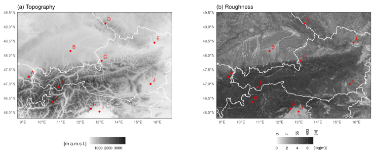
Figure 1: Eastern Alps: topography and topographical roughness—the (logarithm of the) difference between maximum and average elevation in a grid box. Country borders and locations for which seasonal lightning cycles will be shown are added. Details on the specified locations A, B, …, J are given in table 1.

2 Data

The climatology of lightning days is based on lightning detection data from the Austrian Lightning Detection & Information System (ALDIS,  Schulz et al., 2016), complemented by data from the digital elevation model TanDEM-X (Rizzoli et al., 2017) to account for topographic effects.

2.1 Lightning location data

For this study we use ALDIS cloud-to-ground flashes for the summer months April–September. Eleven years of data, 2010–2020, have been on hand. The ALDIS data are cropped slightly to a domain that covers around a quarter of a million square kilometers (Fig. 1). The domain includes the European Eastern Alps and extends northwards to the lower mountain ranges of the Swabian and Franconian Jura and the Bohemian Forest.

	Name	Latitude	Longitude	Elevation [m]	Roughness [m]
A	Saentis	47.2494	9.3433	2214	271
B	Munich	48.1513	11.4921	575	13
C	Gaisberg	47.8056	13.1125	1063	268
D	Bohemian Forest	49.1182	13.3071	1235	100
E	North of Vienna	48.4452	15.8566	268	11
F	Central Alps N	46.8854	10.8672	3593	155
G	Central Alps S	46.3654	10.5872	3213	270
H	Range NE of Udine	46.1327	12.5675	1545	127
I	Udine	46.0301	13.0013	127	5
J	Grazer Becken	46.9968	15.6558	479	49

Table 1: Specifications of locations: The elevation refers to the average of TanDEM-X data in a hexagonal square kilometer. Roughness is defined by the difference between maximum and average TanDEM-X elevations in a hexagon. The letters A, B, …, J are used to mark the locations in Fig. 1.

The spatio-temporal dimensions of a cell used for our climatology are an area of 1 square kilometer and a period of 1 day. The shape of the 1  square kilometer area is taken to be hexagonal and a day is taken to start at 06 UTC, the approximate time of the diurnal lightning minimum. The study region has an area of $248\,308$ km² and the study period from April through November contains 182 days, resulting in approximately 45.2 million spatio-temporal cells for the climatology. For each of these cells the number of years is counted in which “lightning“ occurred, defined as at least one cloud-to-ground discharge. Since the data span the eleven years 2010–2020 this number can in principle lie between 0 amd 11. However, no cell had more than five years in which lightning occurred.

2.2 Digital elevation model

The digital elevation model TanDEM-X (Rizzoli et al., 2017) is used to enhance the data by topographic information. The version used here has a horizontal resolution of 90 m and is aggregated over the unit square kilometer hexagons by taking the mean and the maximum. After aggregation $51$ (out of $248\,308$ unit square kilometer cells) have missing values. They are imputed with the mean of the surrounding values since all of them are over water bodies such as Lake Constance and Lago di Garda.

The natural logarithm of the mean topography (Fig. 1a) will enter the statistical climatology model as explainatory variable. Further, the natural logarithm of the difference between the maxim and the average topography serves as proxy for the roughness of the terrain within a hexagonal square kilometer (Fig. 1b).

3 Methods

Each of the 45.2 million spatio-temporal cells—1 square kilometer hexagons spatially times 1 day temporally for each day from April through October—is one data point for our statistical climatology. Each cell contains the number of observed thunderstorm days over the 11 years for this specific day of the year and hexagonal area. These numbers of observed thunderstorm days $\{0,1,2,\dots,11\}$ can be seen as realizations of Bernoulli’s urn problem with replacement. For each cell, 11 trials are conducted, where each trial has two possible outcomes: lightning and no lightning, respectively.

The outcome of these trials follows a binomial distribution, which is determined by a probability $\pi$ that lightning occurs. In order to estimate the probability $\pi$ of the underlying process, we utilize generalized additive models (GAMs, Wood, 2017) that incoporate data not only for single data points but leverage information of data points with similar settings, e.g. same region, similar time of the year, similar topographic conditions. GAMs have proven their abilities for lightning climatologies in complex terrains (Simon et al., 2017). The GAM used for this study is set up as follows,

$$\text{logit}(\pi)=\beta_{0}+f_{1}(\mathtt{yday})+f_{2}(\mathtt{log\,topo,yday})+f_{3}(\mathtt{lon,lat,yday})+f_{4}(\mathtt{log\,roughness}).$$ (1)

On the left hand side is the logit transformed probability $\pi$. The logit maps the $\pi$ from the probability scale $\left]0,1\right[$ to the real line. On the right hand side is the additive predictor that combines the intercept $\beta_{0}$ of the regression and multiple, potentially non-linear terms $f_{\star}$.

• $f_{1}(\mathtt{yday})$ is a function of the day of the year and thus represents a baseline annual cycle valid for all locations of the domain.

• $f_{2}(\mathtt{log\,topo,yday})$ is a function of the log-topography and the day of the year. Thus this term allows for deviations of the annual cycle from its baseline conditioned on the topography.

• $f_{3}(\mathtt{lon,lat,yday})$ additionally allows deviations from the baseline annual cycle conditioned on the geographical location.

• $f_{4}(\mathtt{log\,roughness})$ adds a correction for the roughness of the topography.

With the GAM all these functions $f_{\star}$ are modelled using regression splines such as cubic regression splines and thin plate regression splines. The spline bases for functions with two ($f_{2}$) or three ($f_{3}$) covariates are set up using the tensor product of the univaraite spline bases. For the technical details on splines within GAMs the reader is refered to Wood (2017).

This setup leads to approximately $2\,500$ regression coefficients of the GAM. These coefficients are estimated via penalized maximum likelihood. Here the amount of smoothing of the potentially non-linear functions $f_{\star}$ is determined by generalized cross-validation as implemented in the mgcv extension for R. Estimating such a flexible regression model for the large data set on hand with $45\,192\,046~{}\text{data\,points}$ is feasible with a fitting algorithm for giga data (Wood et al., 2017, implemented in the mgcv extension for R).

4 Results

Lightning in the eastern Alps is rare. Only 5.47 % of the 45.2 million spatio-temporal cells of 1 km² times 1 day in the 182 days from months April through September had lightning occur in at least one of the eleven years 2010–2020. Fig. 2a shows that the maximum probability for lightning to strike within a grid box of 1 square kilometer on a particular day barely exceeds 2 %. The maps for day 15 of each month demonstrate that the probability of lightning waxes from spring through the end of July and then wanes into autumn. In spring (May 15, top) the likelihood for lightning strikes north of the Alps is regionally uniform below about 0.5 %. The probability along the northern Alpine rim slightly exceeds these values. In the Alps, valleys and mountain ranges stand out (cf. Fig. 1, top) with probabilities in valleys considerably higher than over mountain ranges, which are still mostly snow-covered at this time of the year. By mid-June these differences blur and valleys are almost no longer distinguishable from mountain ranges. By now, lightning in the higher terrain north of the Alps strikes more readily than in the surrounding flat lands. Differences south of the Alps are even starker. The flat land around location I in Fig. 1 has the highest probability in the whole study region. This is exceptional as lower terrain everywhere else has lower probabilities than higher terrain in its vicinity. By mid-July lightning activity favors higher terrain. Lightning probability again clearly differs between valleys and moutain ranges, however now reversed from mid-May. The probability in valleys is considerably lower than over the mountains. Overall, the strongest activity has shifted to the south of the Alpine crest and probabilities even exceed the ones in the former hotspot in the flat land in the vicinity of location F. One month later in mid-August the overall pattern is the same but probabilities are lower—with the exception of location I where the probabilities remain relatively high even into mid-September, by which time lightning activity is low everywhere, most pronouncedly so north of the Alps.

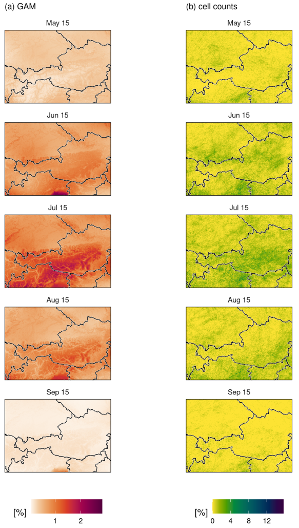
Figure 2: Climatology maps for selected days. a. based on the GAM method, and b. based on the cell-count methods.

Contrary to the results from the GAM-method, results from the cell-count method in Fig. 2b are noisy and lack details despite averaging the results over an 11-day window centered on that particular day. Grid boxes with probabilities of more than 10 % occur next to boxes with 0 %, which necessitated a different color scale in the figure. Only the major features of lower lightning probabilities/frequencies over the high mountains early in the lightning season, the shift into the high mountains and south of the Alpine crest, and the hotspot near location I (Fig. 1) are visible, admittedly more easily so when one has previously seen the results from the GAM-method. Sample sizes in the grid boxes are simply far too small to obtain reliable frequencies of occurrence of lightning, which is a rare event of only about 1 % per day in a 1 square-kilometer grid box. The uncertainty of the cell-count method can be determined using the modified Wilson method (Brown et al., 2001) to estimate the width of the 95 % confidence interval for a binomial distribution (lightning yes/no) for a sample size of 11—the number of years in our data set. The width is a staggering 27 % for an event with a probability of 1 %. Even increasing the sample size by a factor of 11 to $11\times 11=121$ using a time-window of 11 days instead of 1 day as is done in Fig. 2b still yields a width of 4.9 percentage points. Therefore finding a lot of noise in the results from cell-count method comes as no surprise.

The power of the GAM-method and its ability to produce detailed and smooth results even at such high spatial and temporal resolution lies in its harnessing of information from grid boxes that share seasonal, topographical and regional characteristics. Extracting the functional form of these characteristics in turn leads to increased understanding of the contributors to the overall spatio-temporal distribution of the rare event “lightning occurrence”. Fig. 3 shows the effects of each of the additive terms in eq. 1 as they contribute to $\textrm{logit}(\pi)$. Seasonally (Fig. 3a), the probability of lightning for the whole region increases rapidly in spring, tapers off gently in autumn, and slowly increases during main lightning season.

Figure 3: Estimate effects of the GAM: a. the main seasonal cycle $f_{1}$, b. the correction of the seasonal cycle conditioned on the topography, c. the correction of the seasonal cycle given the geographic location, d. the effect of the roughness. All effects contribute to the additive predictor on the logit scale.

The elevation effect (Fig. 3b) varies seasonally. Note that the effect is logarithmic (cf. eq. 1) but the ordinate axis has been labeled in meters to ease interpretation. This effect shows a reduced likelihood for lightning at the highest elevations early in the season, which is reversed in the second half of June. The sign reverses last at the very highest elevations, where snow melts last. Snow-covered ground greatly reduces sensible heat flux and thus the chances for convection to occur. The seasonal elevation effect also changes sign in elevations typical of intra-alpine valleys. It is increased in spring, when the valleys are already free of snow and reduced in summer and early autumn. The very lowest elevations, found mostly at the southern edge of the study region, have an enhanced effect from mid-May on.

The regional effect in Fig. 3c accounts for adjustments needed to add to the effects of season and elevation. At first glance, the patterns do not seem to vary seasonally but a closer look reveals a shift of enhanced and reduced regions from spring into summer and fall. In spring the lightning probability in some parts of the lowlands and rims on either side of the Alps and the high mountains in southeastern Switzerland is enhanced. By mid-July lightning activity along the whole southern side of the Alps is enhanced as well as in the westernmost and easternmost parts of the lowlands north of the Alps. By mid-September, at the end of convective season in most of the region, the northwestern rim and lowlands and especially the southeastern rim and lowlands have enhanced lightning probabilities.

Protruding topography such as peaks increases the likelihood of lightning. Again, the effect is logarithmic but elevation difference in Fig. 3d is given in units of meters. Here the difference between the maximum elevation at 90 m horizontal resolution to the average elevation in the one-square-kilometer grid box serves as proxy for how jagged the terrain is. Overall, where that difference exceeds about 100 m, lightning likelihood increases somewhat, which is in alignment with findings from lightning research (e.g. Rakov and Uman, 2003; Kingfield et al., 2017; Feudale et al., 2013).

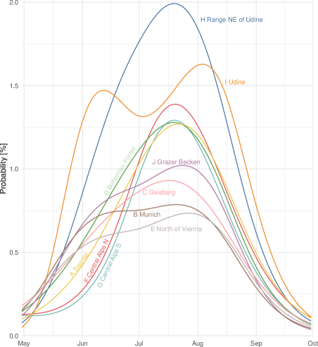
Figure 4: Climatology cycles computed by the GAM for the locations from table 1.

Time series of lightning probability at specific locations in the eastern Alps in Fig. 4 exemplify the sum of the seasonally varying regional and elevation effects and the roughness effect from Fig. 3 and fill in the times between the regional maps of Fig. 2. The lightning season starts about three weeks later at the highest mountains, exemplified by locations F and G, than at other locations (cf. Fig. 1 and Table 1 for their coordinates). The difference in probability between the two locations F and G stems from their difference in elevation. Similar peak probabilities are reached by locations north of the Alps at A (Saentis) and D in the Bohemian Forest, although they are considerably lower. Their seasonal cycles are shifted by about one week, with D starting out one week earlier and A lasting one week longer. Lightning season at location C (Gaisberg), just south of D at the northern rim of the Alps starts about at the same time but peak probabilities are about one third lower. Both A (Saentis) and C (Gaisberg) are locations with a long history of direct lightning measurements from instrumented towers. Although both are at the northern rim of the Alps, seasonally varying regional differences (Fig. 3c) and an elevation difference of 1.1 km result in different shapes and peaks of their seasonal lightning probability distributions. Flat terrain north of the Alps, exemplified by locations B and E, experiences lightning less frequently than the mountainous counterparts A, C and D. They also reach a first peak in probability earlier and then increase slightly to a second peak at the end of July. Locations in the flat lands south of the Alpine crest (E and I) show a similar bimodal distribution. Location I, which is situated in a basin south of the Alps has the most abrupt increase of lightning probability of all 10 locations shown. Despite its low elevation, its peak probabilities exceed the ones of the highest mountains near the Alpine crest. It is located in the hotspot so clearly visible in the regional probability maps in Fig. 2. However, probabilities at location H at the first mountain range north of I are even higher.

5 Discussion and Conclusions

Lightning location systems (LLS) are unique among atmospheric measurement systems in that they provide continuous measurements in both time and space—two-dimensional or three-dimensional depending on LLS type. Since they measure very rare events, translating these measurements into high-resolution climatologies is difficult. Most climatologies so far have used the cell-count method of counting how many flashes occurred within a particular time-space cell, which necessitates making the spatial and/or temporal dimensions of such a cell large in order to achieve a sufficient signal to noise ratio. Frequently cell-sizes of 10–100 square kilometers by 1–12 months have been used (e.g. Schulz et al., 2005; Feudale et al., 2013; Poelman et al., 2016). Bourscheidt et al. (2014); Kingfield et al. (2017); Simon et al. (2017) demonstrated how the cell-count method is unsuitable for smaller cell sizes corroborating the theoretical considerations in Diendorfer (2008), who used the Poisson distribution to derive the minimum number of flashes in a cell required for reaching a specified accuracy. The Poisson distribution is the limiting case of the binomial distribution, which describes the binary event of the occurrence of lightning (yes/no). We therefore use the binomial distribution to compute the 95 % confidence interval for a lightning probability of 1 %. It has a width of staggering 27 % for a sample size of 11 for a particular day in our 11-year data set. Increasing the time dimension of a cell from 1 day to averaging over 11 days to obtain a sample size of 121 still gives an uncertainty of 4.9 %, five times larger than what we need to detect. Fig. 2b illustrates the high noise level the cell-count method produces for high-resolution cells of 1 km² times 1 day. Fig. 2a, on the other hand, produced with the generalized additive model (GAM) method, is devoid of noise and yet provides intricate spatial details for any given day in the lightning season (of which the map shows five). Similarly spatially detailed climatological maps can be achieved using a bivariate Gaussian error distribution for each lightning discharge instead of a precise location (Bourscheidt et al., 2014; Kingfield et al., 2017). The advantage of the GAM method is its ability to harness regional, elevational and seasonal characteristics that cells share that need not be immediately “next” to another and thus make a high combined spatio-temporal resolution possible. To our knowledge, this paper presents the first daily-resolved kilometer-scale lightning climatology over a large region. GAMs have another advantage: the resulting functional forms of characteristics shared among cells. Fig. 3 yield insights about the processes contributing to the final climatological result.

The purely seasonal effect (Fig. 3a) shows a rapid increase of ligthning probability in late spring but a more gradual tapering off in late summer and early fall, which was previously also found for a smaller region in the eastern Alps (Simon et al., 2017). The peak, however, is less sinusoidal but more plateau-like, probably due to the larger region where different subdomains peak at different times (cf. Fig. 4.

Lightning probability also varies with elevation (Fig. 3b). Smorgonskiy et al. (2013); Simon et al. (2017) found an overall increase with elevation. The GAM method allowed to implement a seasonally varying elevation effect and found an increased probability in spring at elevations in lowlands and intra-Alpine valleys compared to higher elevations (above approx. 1200 m msl), which are still (partly) snow covered. This pattern reverses later and high elevations have a higher probability when the snow has melted. The most pronounced increase is at the very lowest elevations found on the southern side of the Alps (vicinity of location I) with maxima in June and late August/early September.

This regional hotspot was already known from earlier cell-count climatolgies (e.g. Schulz et al., 2005; Feudale et al., 2013; Taszarek et al., 2019). With GAMs we could additionally identify how the regional differences vary with season—in extension to Simon et al. (2017)—when different elevations are already accounted for.

The approach of using similar characteristics to compute high-resolution yet non-noisy lightning climatologies with GAMs pioneered by Simon et al. (2017) can be expanded by including further characteristics beyond region, elevation and time of year. Snow cover could be explicitly included since it suppresses convection. In our analysis it is implicitly contained in the seasonally varying elevation effect where lightning season at the highest elevations with the longest snow cover duration has a delayed start. Further characteristics of earth’s surface such as slope angle and exposure, soil moisture, amount and type of vegetation cover, and land/water could be included as well as the presence of tall structures, which can trigger lightning (Rakov and Uman, 2003). The GAM approach can also use further additive terms with output from numerical weather prediction models in order to provide forecasts of the probability of thunderstorm occurrence (Simon et al., 2018).

Computational Details

The results in this study were achieved using R, a software environment for statistical computing and graphics. The add-on packages mgcv were used for building the statistical model.

Statements and Declarations

The authors declare that they have no conflicts of interest.

References

- Becerra et al. (2018) Becerra M, Long M, Schulz W, Thottappillil R (2018). “On the Estimation of the Lightning Incidence to Offshore Wind Farms.” Electric Power Systems Research, 157, 211–226. 10.1016/j.epsr.2017.12.008.
- Bourscheidt et al. (2014) Bourscheidt V, Pinto O, Naccarato KP (2014). “Improvements on Lightning Density Estimation Based on Analysis of Lightning Location System Performance Parameters: Brazilian Case.” IEEE Transactions on Geoscience and Remote Sensing, 52(3), 1648–1657. 10.1109/tgrs.2013.2253109.
- Brown et al. (2001) Brown LD, Cai TT, DasGupta A (2001). “Interval Estimation for a Binomial Proportion.” Statistical Science, 16(2), nil. 10.1214/ss/1009213286.
- Cummins et al. (1998) Cummins K, Krider E, Malone M (1998). “The US National Lightning Detection Network and Applications of Cloud-to-Ground Lightning Data by Electric Power Utilities.” IEEE Transactions on Electromagnetic Compatibility, 40(4), 465–480. 10.1109/15.736207.
- Diendorfer (2008) Diendorfer G (2008). “Some comments on the achievable accuracy of local ground flash density values.” In 29th International Conference on Lightning Protection, 23-26 June 2008, Uppsala, Sweden.
- Dowdy and Mills (2012) Dowdy AJ, Mills GA (2012). “Atmospheric and Fuel Moisture Characteristics Associated With Lightning-Attributed Fires.” Journal of Applied Meteorology and Climatology, 51(11), 2025–2037. 10.1175/jamc-d-11-0219.1.
- Feudale et al. (2013) Feudale L, Manzato A, Micheletti S (2013). “A Cloud-to-Ground Lightning Climatology for North-Eastern Italy.” Adv. Sci. Res., 10(1), 77–84. 10.5194/asr-10-77-2013.
- Holle (2016) Holle RL (2016). “A Summary of Recent National-Scale Lightning Fatality Studies.” Weather, Climate, and Society, 8(1), 35–42. 10.1175/WCAS-D-15-0032.1.
- Kingfield et al. (2017) Kingfield DM, Calhoun KM, de Beurs KM (2017). “Antenna Structures and Cloud-To-Ground Lightning Location: 1995-2015.” Geophysical Research Letters, 44(10), 5203–5212. 10.1002/2017gl073449.
- Montanyà et al. (2014) Montanyà J, van der Velde O, Williams ER (2014). “Lightning Discharges Produced By Wind Turbines.” Journal of Geophysical Research: Atmospheres, 119(3), 1455–1462. 10.1002/2013jd020225.
- Murray (2016) Murray LT (2016). “Lightning NOx and Impacts on Air Quality.” Current Pollution Reports, 2(2), 115–133. 10.1007/s40726-016-0031-7.
- Poelman et al. (2016) Poelman DR, Schulz W, Diendorfer G, Bernardi M (2016). “The European Lightning Location System EUCLID—Part 2: Observations.” Natural Hazards and Earth System Sciences, 16(2), 607–616. 10.5194/nhess-16-607-2016.
- Rakov and Uman (2003) Rakov VA, Uman MA (2003). Lightning: Physics and Effects. Cambridge University Press. 10.1017/CBO9781107340886.
- Reineking et al. (2010) Reineking B, Weibel P, Conedera M, Bugmann H (2010). “Environmental Determinants of Lightning- v. Human-Induced Forest Fire Ignitions Differ in a Temperate Mountain Region of Switzerland.” International Journal of Wildland Fire, 19(5), 541–557. 10.1071/WF08206.
- Ritenour et al. (2008) Ritenour AE, Morton MJ, McManus JG, Barillo DJ, Cancio LC (2008). “Lightning Injury: A Review.” Burns, 34(5), 585–594. 10.1016/j.burns.2007.11.006.
- Rizzoli et al. (2017) Rizzoli P, Martone M, Gonzalez C, Wecklich C, Borla Tridon D, Bräutigam B, Bachmann M, Schulze D, Fritz T, Huber M, Wessel B, Krieger G, Zink M, Moreira A (2017). “Generation and performance assessment of the global TanDEM-X digital elevation model.” ISPRS Journal of Photogrammetry and Remote Sensing, 132, 119–139. 10.1016/j.isprsjprs.2017.08.008.
- Schulz et al. (2005) Schulz W, Cummins K, Diendorfer G, Dorninger M (2005). “Cloud-to-ground lightning in Austria: A 10-year study using data from a lightning location system.” J. Geophys. Res., 110, D09101—-. 10.1029/2004JD005332.
- Schulz et al. (2016) Schulz W, Diendorfer G, Pedeboy S, Poelman DR (2016). “The European Lightning Location System EUCLID Part 1: Performance Analysis and Validation.” Natural Hazards and Earth System Sciences, 16(2), 595–605. 10.5194/nhess-16-595-2016.
- Simon et al. (2018) Simon T, Fabsic P, Mayr GJ, Umlauf N, Zeileis A (2018). “Probabilistic Forecasting of Thunderstorms in the Eastern Alps.” Mon. Wea. Rev., 146(9), 2999–3009. 10.1175/MWR-D-17-0366.1.
- Simon et al. (2017) Simon T, Umlauf N, Zeileis A, Mayr GJ, Schulz W, Diendorfer G (2017). “Spatio-Temporal Modelling of Lightning Climatologies for Complex Terrain.” Nat. Hazards Earth Syst. Sci., 17(3), 305–314. 10.5194/nhess-17-305-2017.
- Smorgonskiy et al. (2013) Smorgonskiy A, Rachidi F, Rubinstein M, Diendorfer G (2013). “On the relation between lightning flash density and terrain elevation.” In 2013 International Symposium on Lightning Protection (XII SIPDA), p. nil. 10.1109/sipda.2013.6729216.
- Taszarek et al. (2019) Taszarek M, Allen J, Púčik T, Groenemeijer P, Czernecki B, Kolendowicz L, Lagouvardos K, Kotroni V, Schulz W (2019). “A Climatology of Thunderstorms across Europe from a Synthesis of Multiple Data Sources.” J. Climate, 32(6), 1813–1837. 10.1175/JCLI-D-18-0372.1.
- Wapler (2013) Wapler K (2013). “High-Resolution Climatology of Lightning Characteristics within Central Europe.” Meteor. Atmos. Phys., 122(3-4), 175–184. 10.1007/s00703-013-0285-1.
- Wood (2017) Wood SN (2017). Generalized Additive Models: An Introduction with R. Texts in Statistical Science, 2nd edition. Chapman & Hall/CRC, Boca Raton.
- Wood et al. (2017) Wood SN, Li Z, Shaddick G, Augustin NH (2017). “Generalized Additive Models for Gigadata: Modeling the U.K. Black Smoke Network Daily Data.” Journal of the American Statistical Association, 112(519), 1199–1210. 10.1080/01621459.2016.1195744.